Speech Recognition and Hidden Markov Models

CPSC4600@UTC/CSE

Hidden Markov models

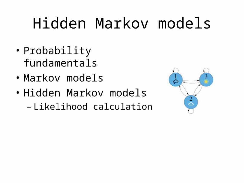
• Probability fundamentals

• Markov models

• Hidden Markov models– Likelihood calculation

Probability fundamentals

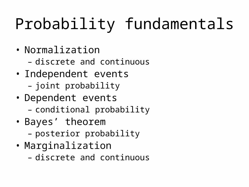
• Normalization– discrete and continuous

• Independent events– joint probability

• Dependent events– conditional probability

• Bayes’ theorem– posterior probability

• Marginalization– discrete and continuous

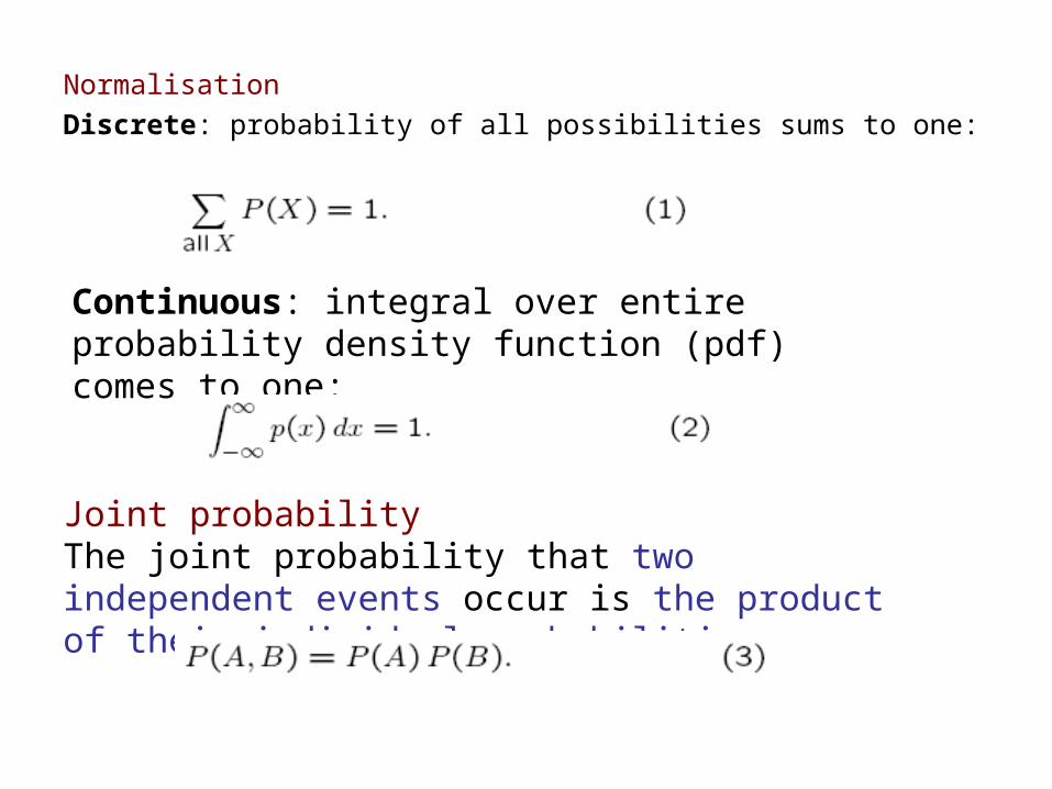
Normalisation

Discrete: probability of all possibilities sums to one:

Continuous: integral over entire probability density function (pdf) comes to one:

Joint probabilityThe joint probability that two independent events occur is the product of their individual probabilities:

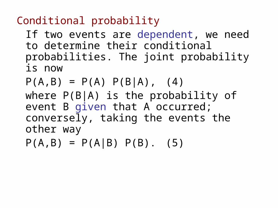
Conditional probabilityIf two events are dependent, we need to determine their conditional probabilities. The joint probability is now

P(A,B) = P(A) P(B|A), (4)where P(B|A) is the probability of event B given that A occurred; conversely, taking the events the other way

P(A,B) = P(A|B) P(B). (5)

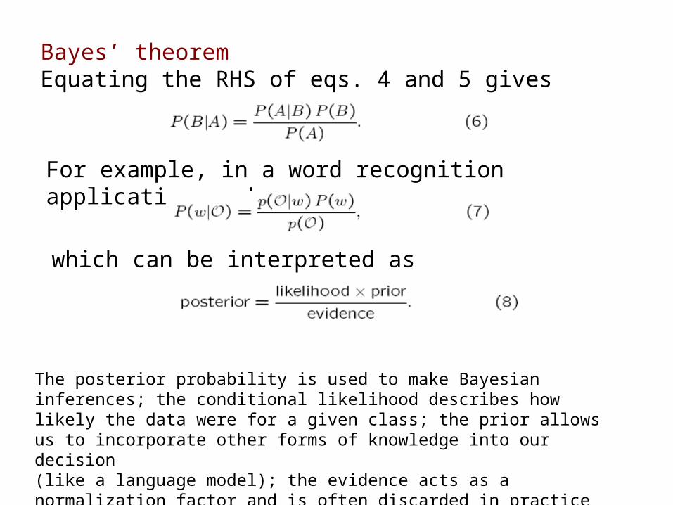
Bayes’ theoremEquating the RHS of eqs. 4 and 5 gives

For example, in a word recognition application we have

which can be interpreted as

The posterior probability is used to make Bayesian inferences; the conditional likelihood describes how likely the data were for a given class; the prior allows us to incorporate other forms of knowledge into our decision(like a language model); the evidence acts as a normalization factor and is often discarded in practice (as it is the same for all classes).

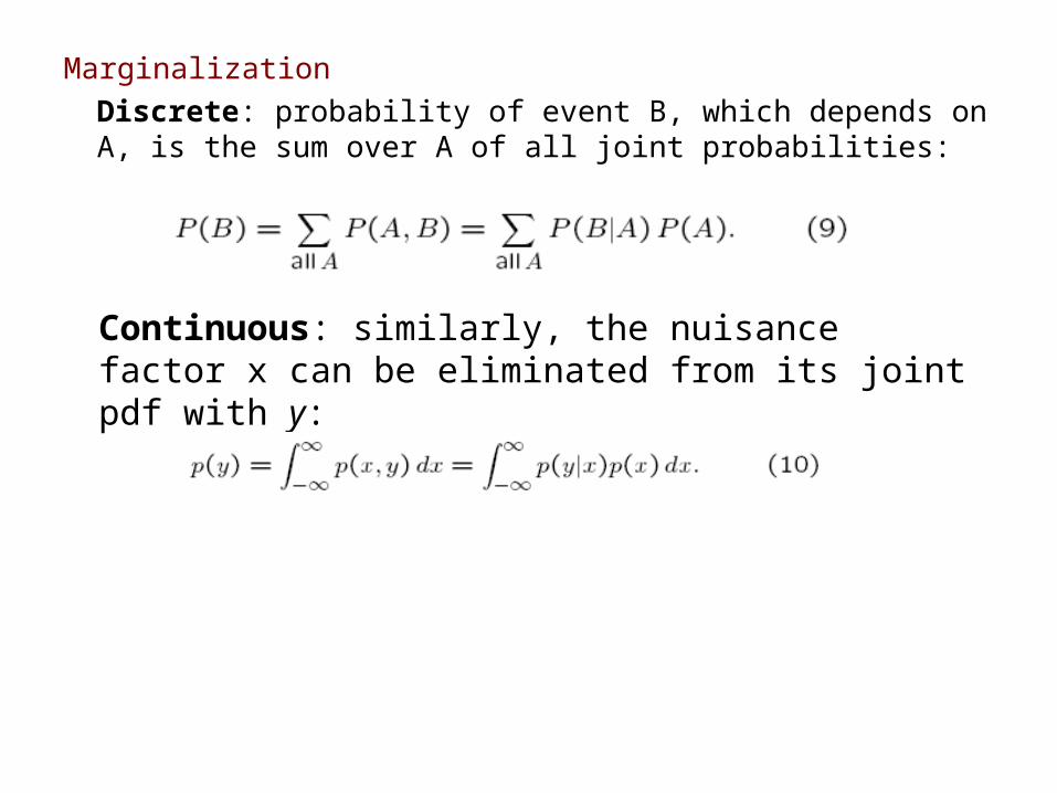
Marginalization

Discrete: probability of event B, which depends on A, is the sum over A of all joint probabilities:

Continuous: similarly, the nuisance factor x can be eliminated from its joint pdf with y:

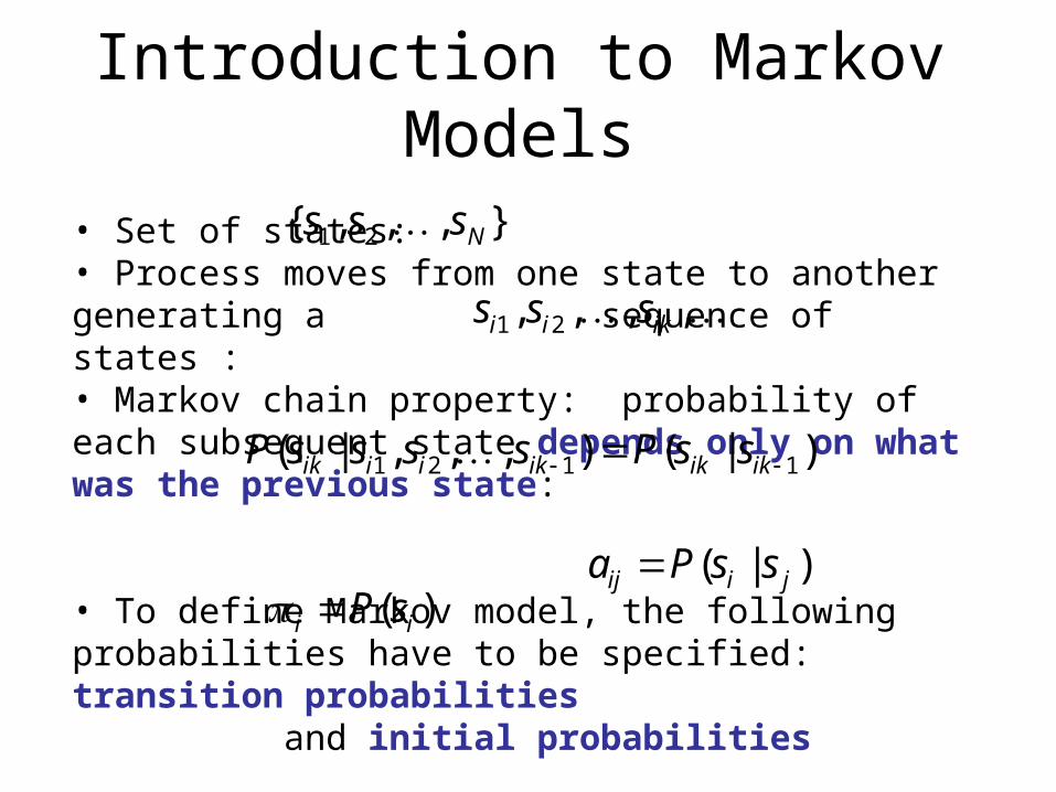
• Set of states: • Process moves from one state to another generating a

sequence of states : • Markov chain property: probability of each subsequent state depends only on what was the previous state:

• To define Markov model, the following probabilities have to be specified: transition probabilities and initial probabilities

Introduction to Markov Models

},,,{ 21 Nsss

,,,, 21 ikii sss

)|(),,,|( 1121 ikikikiiik ssPssssP

)|( jiij ssPa )( ii sP

Rain Dry

0.70.3

0.2 0.8

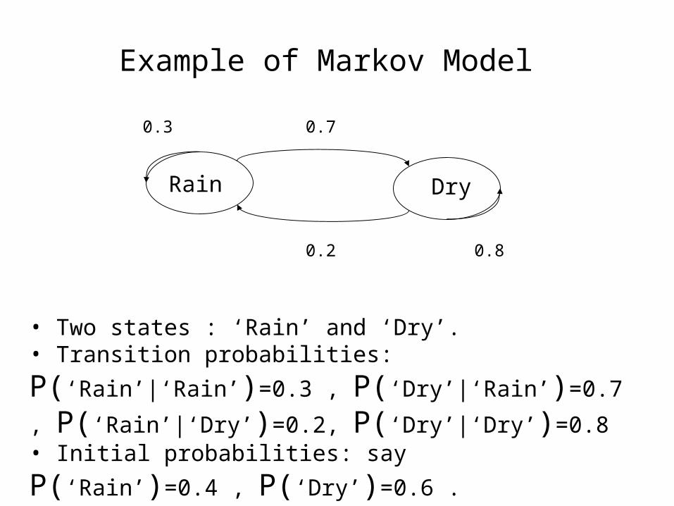
• Two states : ‘Rain’ and ‘Dry’.• Transition probabilities: P(‘Rain’|‘Rain’)=0.3 ,

P(‘Dry’|‘Rain’)=0.7 , P(‘Rain’|‘Dry’)=0.2, P(‘Dry’|‘Dry’)=0.8

• Initial probabilities: say P(‘Rain’)=0.4 , P(‘Dry’)=0.6 .

Example of Markov Model

• By Markov chain property, probability of state sequence can be found by the formula:

• Suppose we want to calculate a probability of a sequence of states in our example, {‘Dry’,’Dry’,’Rain’,Rain’}.

P({‘Dry’,’Dry’,’Rain’,Rain’} ) =P(‘Rain’|’Rain’) P(‘Rain’|’Dry’) P(‘Dry’|’Dry’) P(‘Dry’)= = 0.3*0.2*0.8*0.6

Calculation of sequence probability

)()|()|()|(

),,,()|(

),,,(),,,|(),,,(

112211

1211

12112121

iiiikikikik

ikiiikik

ikiiikiiikikii

sPssPssPssP

sssPssP

sssPssssPsssP

Hidden Markov models.

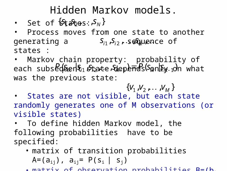
• Set of states: • Process moves from one state to another generating a

sequence of states :• Markov chain property: probability of each subsequent state depends only on what was the previous state:

• States are not visible, but each state randomly generates one of M observations (or visible states)• To define hidden Markov model, the following probabilities have to be specified:

• matrix of transition probabilities A=(aij), aij= P(si | sj)

• matrix of observation probabilities B=(bi (vm )), bi(vm ) = P(vm

| si) • initial probabilities =(i), i = P(si) . Model is represented

by M=(A, B, ).

},,,{ 21 Nsss

,,,, 21 ikii sss

)|(),,,|( 1121 ikikikiiik ssPssssP

},,,{ 21 Mvvv

Low High

0.70.3

0.2 0.8

DryRain

0.6

0.60.4 0.4

Example of Hidden Markov Model

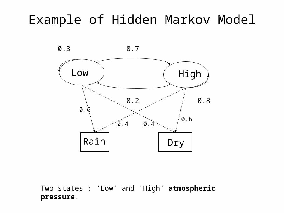
Two states : ‘Low’ and ‘High’ atmospheric pressure.

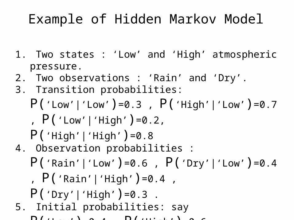
1. Two states : ‘Low’ and ‘High’ atmospheric pressure.2. Two observations : ‘Rain’ and ‘Dry’.

3. Transition probabilities: P(‘Low’|‘Low’)=0.3 ,

P(‘High’|‘Low’)=0.7 , P(‘Low’|‘High’)=0.2,

P(‘High’|‘High’)=0.8

4. Observation probabilities : P(‘Rain’|‘Low’)=0.6 ,

P(‘Dry’|‘Low’)=0.4 , P(‘Rain’|‘High’)=0.4 ,

P(‘Dry’|‘High’)=0.3 .

5. Initial probabilities: say P(‘Low’)=0.4 , P(‘High’)=0.6 .

Example of Hidden Markov Model

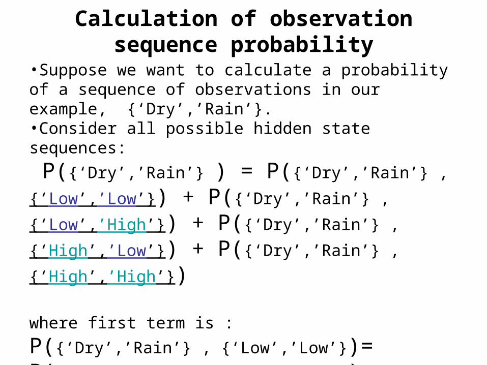
•Suppose we want to calculate a probability of a sequence of observations in our example, {‘Dry’,’Rain’}.•Consider all possible hidden state sequences:

P({‘Dry’,’Rain’} ) = P({‘Dry’,’Rain’} , {‘Low’,’Low’}) + P({‘Dry’,’Rain’} , {‘Low’,’High’}) + P({‘Dry’,’Rain’} ,

{‘High’,’Low’}) + P({‘Dry’,’Rain’} , {‘High’,’High’})

where first term is :

P({‘Dry’,’Rain’} , {‘Low’,’Low’})= P({‘Dry’,’Rain’} | {‘Low’,’Low’}) P({‘Low’,’Low’}) = P(‘Dry’|’Low’)P(‘Rain’|’Low’) P(‘Low’)P(‘Low’|’Low)= 0.4*0.6*0.4*0.3

Calculation of observation sequence probability

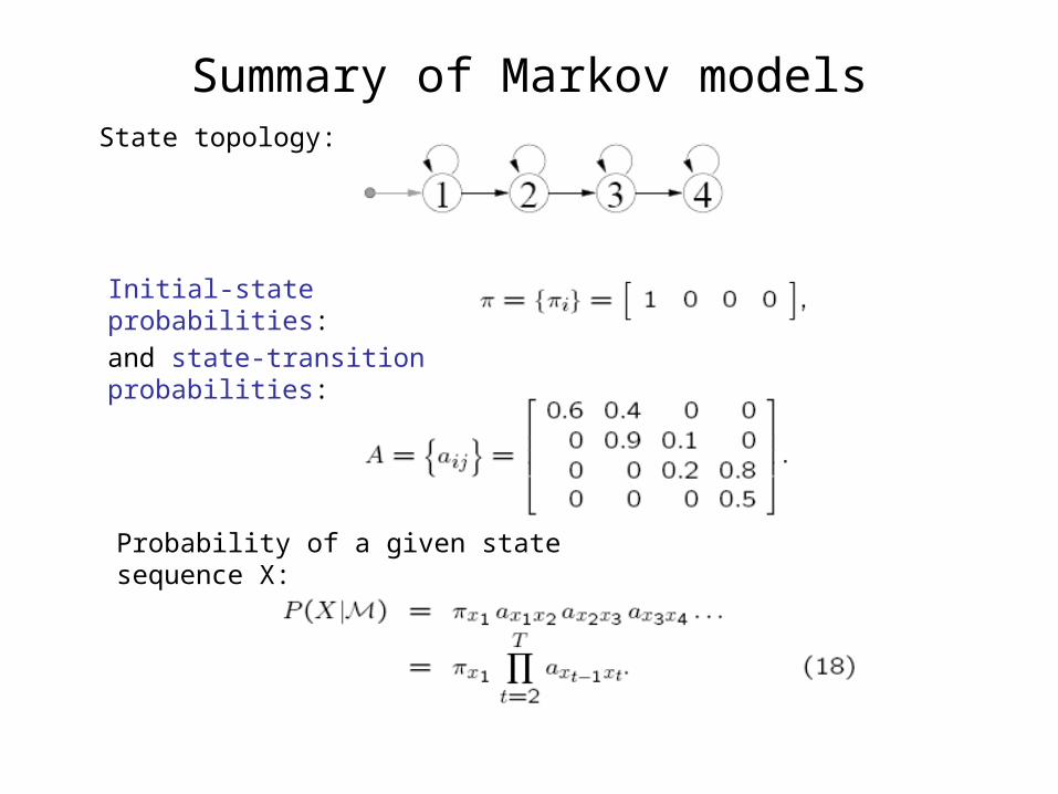
Summary of Markov modelsState topology:

Initial-state probabilities:

and state-transition probabilities:

Probability of a given state sequence X:

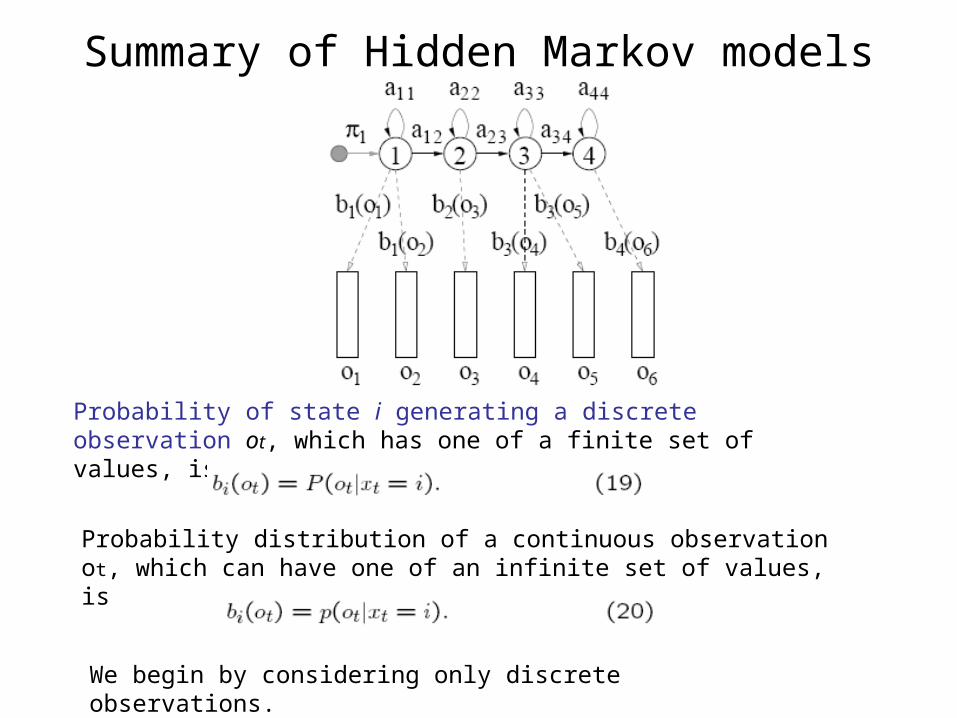
Summary of Hidden Markov models

Probability of state i generating a discrete observation ot, which has one of a finite set of values, is

Probability distribution of a continuous observation ot, which can have one of an infinite set of values, is

We begin by considering only discrete observations.

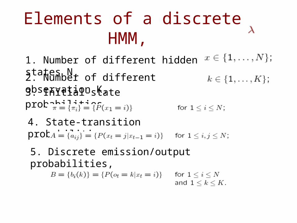
Elements of a discrete HMM,

1. Number of different hidden states N,

2. Number of different observation K,

3. Initial-state probabilities,

4. State-transition probabilities,

5. Discrete emission/output probabilities,

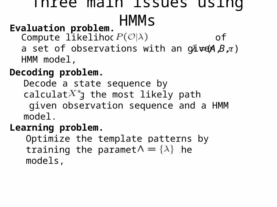
Evaluation problem.

Decoding problem.

Learning problem.

Three main issues using HMMs

Compute likelihood of a set of observations with an given HMM model,

(A,B, )

Decode a state sequence by calculating the most likely path given observation sequence and a HMM model.

Optimize the template patterns by training the parameters in the models,

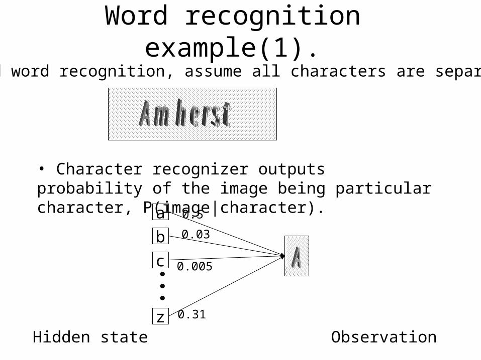
• Typed word recognition, assume all characters are separated.

• Character recognizer outputs probability of the image being particular character, P(image|character).

0.5

0.03

0.005

0.31z

c

b

a

Word recognition example(1).

Hidden state Observation

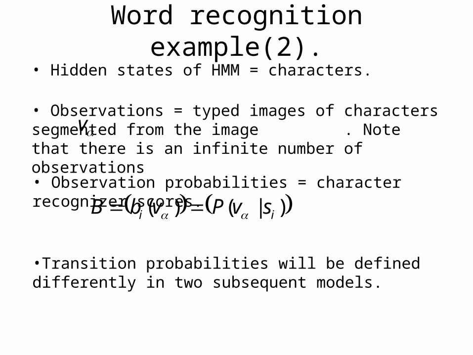
• Hidden states of HMM = characters.

• Observations = typed images of characters segmented from the image . Note that there is an infinite number of observations

• Observation probabilities = character recognizer scores.

•Transition probabilities will be defined differently in two subsequent models.

Word recognition example(2).

)|()( ii svPvbB

v

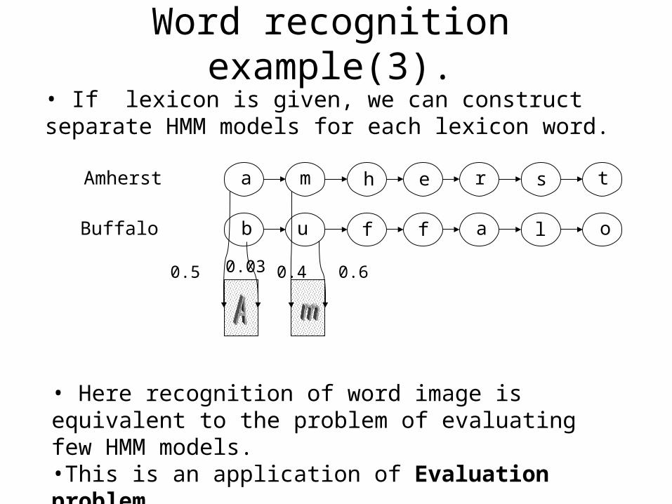
• If lexicon is given, we can construct separate HMM models for each lexicon word.

Amherst a m h e r s t

Buffalo b u f f a l o

0.5 0.03

• Here recognition of word image is equivalent to the problem of evaluating few HMM models.•This is an application of Evaluation problem.

Word recognition example(3).

0.4 0.6

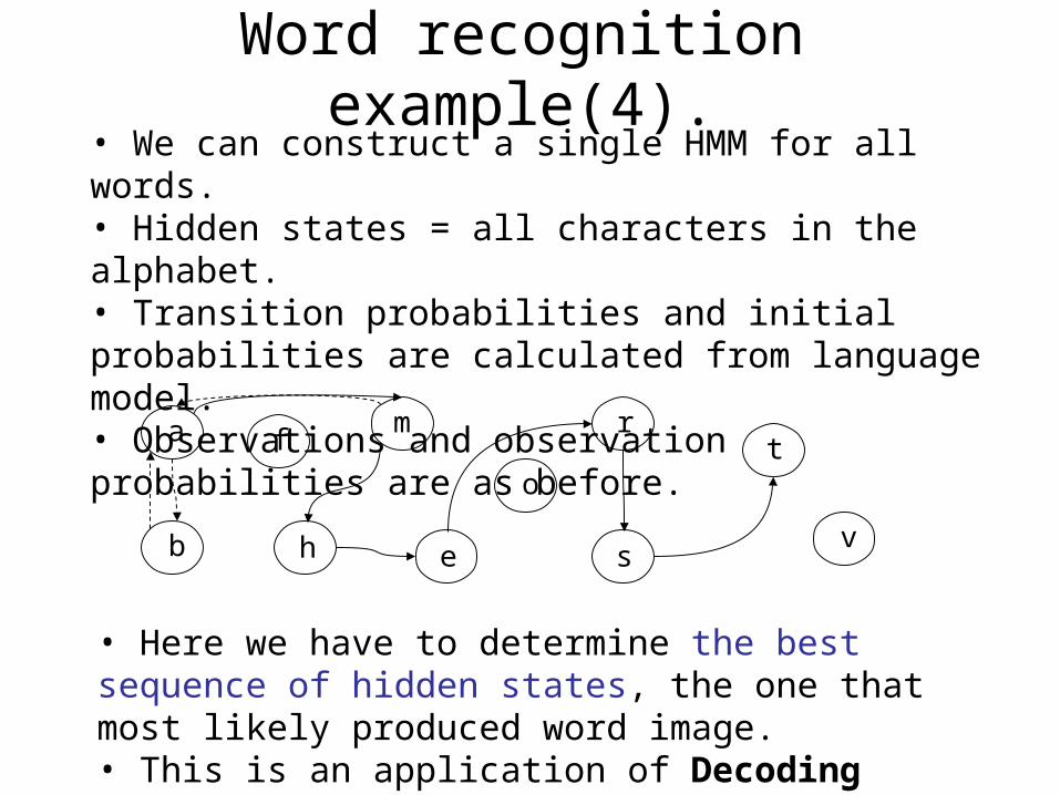
• We can construct a single HMM for all words.• Hidden states = all characters in the alphabet.• Transition probabilities and initial probabilities are calculated from language model.• Observations and observation probabilities are as before.

a m

h e

r

s

t

b v

f

o

• Here we have to determine the best sequence of hidden states, the one that most likely produced word image.• This is an application of Decoding problem.

Word recognition example(4).

Task 1: Likelihood of an Observation Sequence

• What is ?• The likelihood of an observation sequence is the

sum of the probabilities of all possible state sequences in the HMM.

• Naïve computation is very expensive. Given T observations and N states, there are NT possible state sequences.

• Even small HMMs, e.g. T=10 and N=10, contain 10 billion different paths

• Solution to this and Task 2 is to use dynamic programming

P(O | )

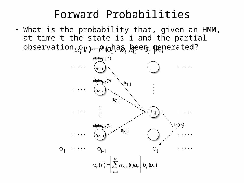
Forward Probabilities• What is the probability that, given an HMM, at time t the

state is i and the partial observation o1 … ot has been generated?

t (i) P(o1...ot , qt si | )

t ( j) t 1(i)aiji1

N

b j (ot )

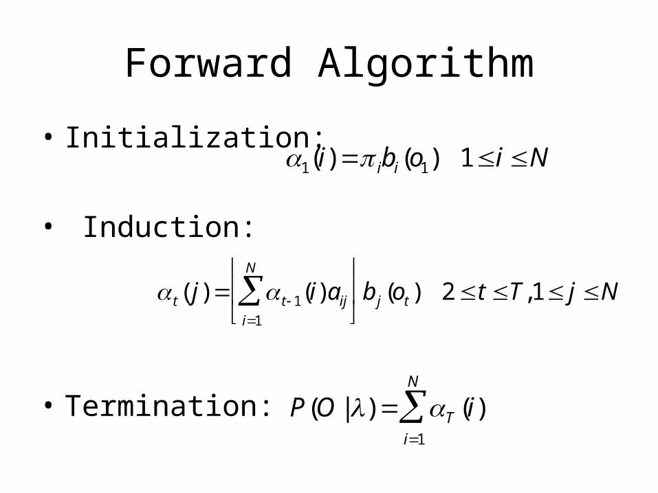
Forward Algorithm

• Initialization:

• Induction:

• Termination:

t ( j) t 1(i)aiji1

N

b j (ot ) 2 t T,1 j N

1(i) ibi(o1) 1iN

P(O | ) T (i)i1

N

Forward Algorithm Complexity

• In the naïve approach to solving problem 1 it takes on the order of 2T*NT computations

• The forward algorithm takes on the order of N2T computations

• The structure of hidden states is chosen.

• Observations are feature vectors extracted from vertical slices.

• Probabilistic mapping from hidden state to feature vectors: 1. use mixture of Gaussian models2. Quantize feature vector space.

Character recognition with HMM example

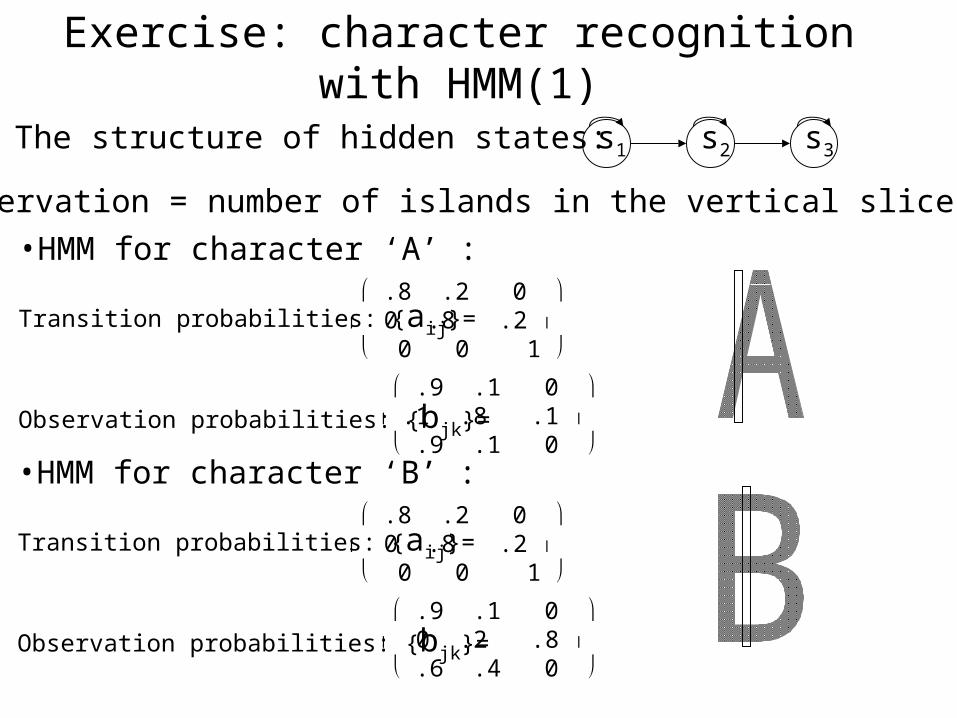
• The structure of hidden states:

• Observation = number of islands in the vertical slice.

s1 s2 s3

•HMM for character ‘A’ :

Transition probabilities: {aij}=

Observation probabilities: {bjk}=

.8 .2 0 0 .8 .2 0 0 1

.9 .1 0 .1 .8 .1 .9 .1 0

•HMM for character ‘B’ :

Transition probabilities: {aij}=

Observation probabilities: {bjk}=

.8 .2 0 0 .8 .2 0 0 1

.9 .1 0 0 .2 .8 .6 .4 0

Exercise: character recognition with HMM(1)

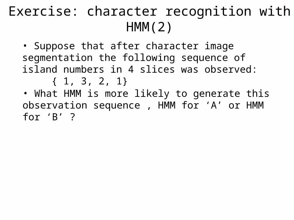
• Suppose that after character image segmentation the following sequence of island numbers in 4 slices was observed: { 1, 3, 2, 1}

• What HMM is more likely to generate this observation sequence , HMM for ‘A’ or HMM for ‘B’ ?

Exercise: character recognition with HMM(2)

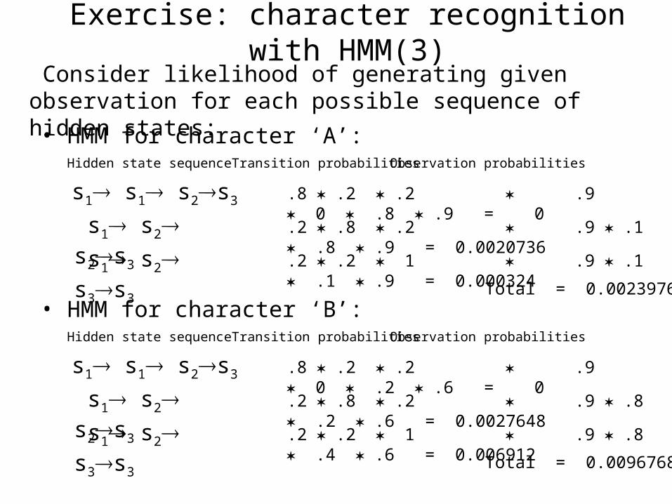
Consider likelihood of generating given observation for each possible sequence of hidden states:

• HMM for character ‘A’:Hidden state sequence Transition probabilities Observation probabilities

s1 s1 s2s3 .8 .2 .2 .9 0 .8 .9 = 0

s1 s2 s2s3 .2 .8 .2 .9 .1 .8 .9 = 0.0020736

s1 s2 s3s3 .2 .2 1 .9 .1 .1 .9 = 0.000324

Total = 0.0023976 • HMM for character ‘B’:

Hidden state sequence Transition probabilities Observation probabilities

s1 s1 s2s3 .8 .2 .2 .9 0 .2 .6 = 0

s1 s2 s2s3 .2 .8 .2 .9 .8 .2 .6 = 0.0027648

s1 s2 s3s3 .2 .2 1 .9 .8 .4 .6 = 0.006912

Total = 0.0096768

Exercise: character recognition with HMM(3)

Task 2: Decoding

• The solution to Task 1 (Evaluation) gives us the sum of all paths through an HMM efficiently.

• For Task 2, we want to find the path with the highest probability.

• We want to find the state sequence Q=q1…qT, such that

QargmaxQ '

P(Q' |O,)

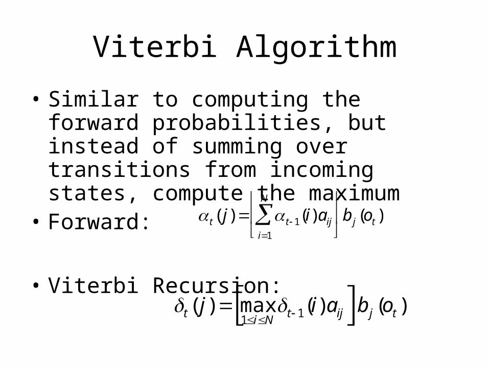
Viterbi Algorithm

• Similar to computing the forward probabilities, but instead of summing over transitions from incoming states, compute the maximum

• Forward:

• Viterbi Recursion:

t ( j) t 1(i)aiji1

N

b j (ot )

t ( j) max1iN

t 1(i)aij b j (ot )

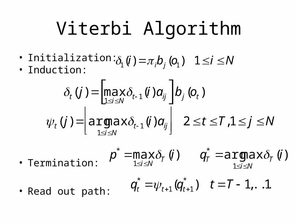
Viterbi Algorithm

• Initialization:• Induction:

• Termination:

• Read out path:

1(i) ib j (o1) 1iN

t ( j) max1iN

t 1(i)aij b j (ot )

t ( j) argmax1iN

t 1(i)aij

2 t T,1 j N

p* max1iN

T (i)

qT* argmax

1iNT (i)

qt* t1(qt1

* ) t T 1,...,1

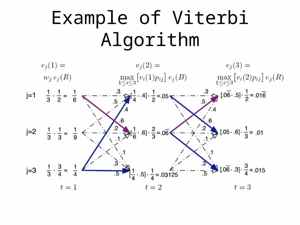
Example of Viterbi Algorithm

Voice Biometrics

General Description

• Each individual has individual voice components called phonemes. Each phoneme has a pitch, cadence, and inflection

• These three give each one of us a unique voice sound.

• The similarity in voice comes from cultural and regional influences in the form of accents.

• Voice physiological and behavior biometric are influenced by our body, environment, and age.

Voice Capture

• Voice can be captured in two ways:– Dedicated resource like a microphone– Existing infrastructure like a telephone

• Captured voice is influenced by two factors:– Quality of the recording device– The recording environment

• In wireless communication, voice travels through open air and then through terrestrial lines, it therefore, suffers from great interference.

Application of Voice Technology

• Voice technology is applicable in a variety of areas. Those used in biometric technology include:– Voice Verification

• Internet/intranet security: – on-line banking – on-line security trading – access to corporate databases – on-line information services

• PC access restriction software

Voice Verification

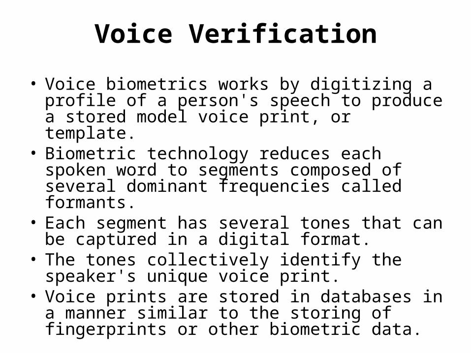
• Voice biometrics works by digitizing a profile of a person's speech to produce a stored model voice print, or template.

• Biometric technology reduces each spoken word to segments composed of several dominant frequencies called formants.

• Each segment has several tones that can be captured in a digital format.

• The tones collectively identify the speaker's unique voice print.

• Voice prints are stored in databases in a manner similar to the storing of fingerprints or other biometric data.

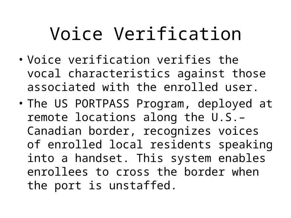
• Voice verification verifies the vocal characteristics against those associated with the enrolled user.

• The US PORTPASS Program, deployed at remote locations along the U.S.–Canadian border, recognizes voices of enrolled local residents speaking into a handset. This system enables enrollees to cross the border when the port is unstaffed.

Voice Verification

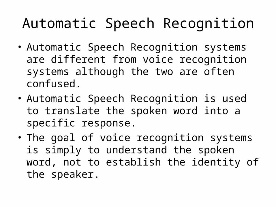
• Automatic Speech Recognition systems are different from voice recognition systems although the two are often confused.

• Automatic Speech Recognition is used to translate the spoken word into a specific response.

• The goal of voice recognition systems is simply to understand the spoken word, not to establish the identity of the speaker.

Automatic Speech Recognition

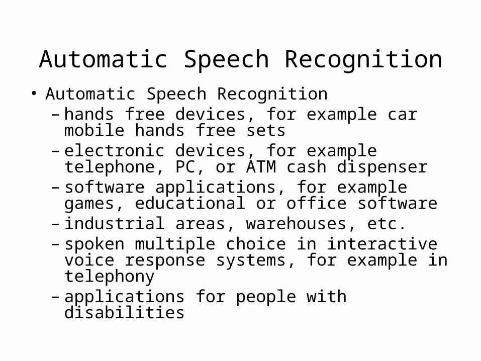
• Automatic Speech Recognition– hands free devices, for example car mobile

hands free sets – electronic devices, for example telephone,

PC, or ATM cash dispenser – software applications, for example games,

educational or office software – industrial areas, warehouses, etc. – spoken multiple choice in interactive voice

response systems, for example in telephony – applications for people with disabilities

Automatic Speech Recognition

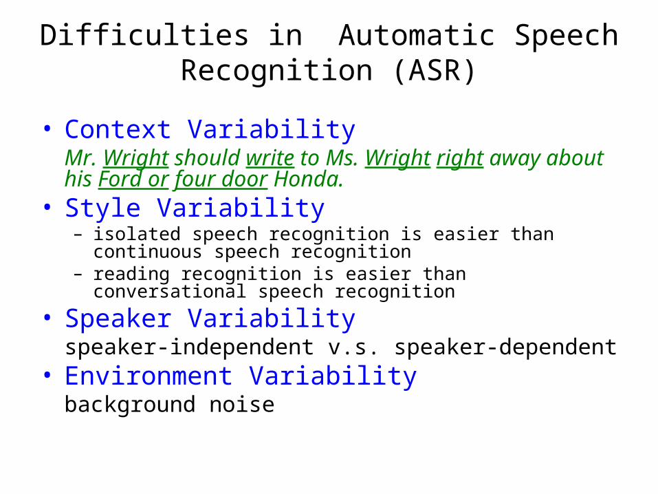
Difficulties in Automatic Speech Recognition (ASR)

• Context VariabilityMr. Wright should write to Ms. Wright right away about his Ford or four door Honda.

• Style Variability– isolated speech recognition is easier than continuous speech

recognition– reading recognition is easier than conversational speech

recognition

• Speaker Variabilityspeaker-independent v.s. speaker-dependent

• Environment Variabilitybackground noise

Task of ASR

The task of speech recognition is to take as input an acoustic waveform and produce as output a string of words.

Acoustic Processing of Speech

Two important characteristics of a wave• Frequency and Pitch

– The frequency is the number of times per second that a wave repeats itself, or cycles.

– Unit: cycles per second are usually called Hertz (Hz)– The pitch is the perceptual correlate of frequency

• Amplitude and loudness– The amplitude measures the amount of air pressure

variation.– Loudness is the perceptual correlate of the power,

which is related to the square of the amplitude.

Acoustic Processing of Speech

Feature extraction• Analog-to-digital conversion

– Sampling: In order to accurately measure a wave, it is necessary to have at least two samples in each cycle

• One measuring the positive part of the wave• The other one measuring the negative part• Thus the maximum frequency wave that can be measured is

one whose frequency is half the sample rate.• This maximum frequency for a given sampling rate is called

the Nyquist frequency.

– Quantization: Representing a real-valued number as an integer.

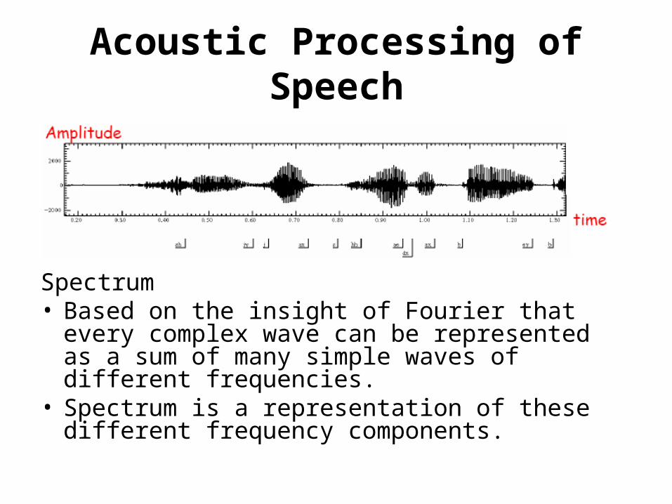
Acoustic Processing of Speech

Spectrum• Based on the insight of Fourier that every

complex wave can be represented as a sum of many simple waves of different frequencies.

• Spectrum is a representation of these different frequency components.

Acoustic Processing of Speech

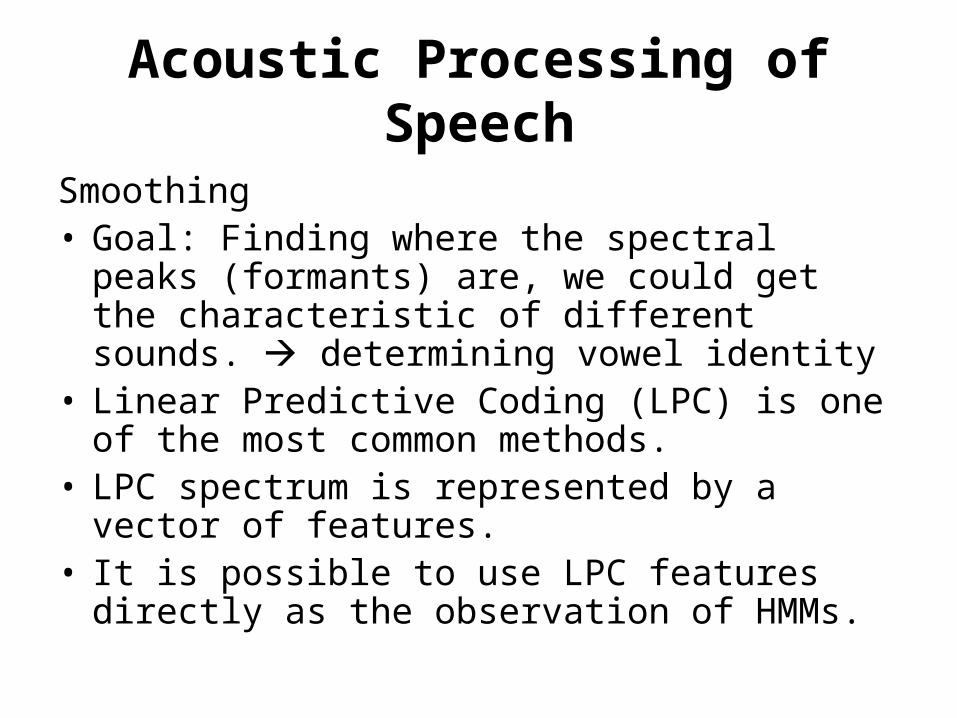
Smoothing• Goal: Finding where the spectral peaks

(formants) are, we could get the characteristic of different sounds. determining vowel identity

• Linear Predictive Coding (LPC) is one of the most common methods.

• LPC spectrum is represented by a vector of features.

• It is possible to use LPC features directly as the observation of HMMs.

Acoustic Processing of Speech

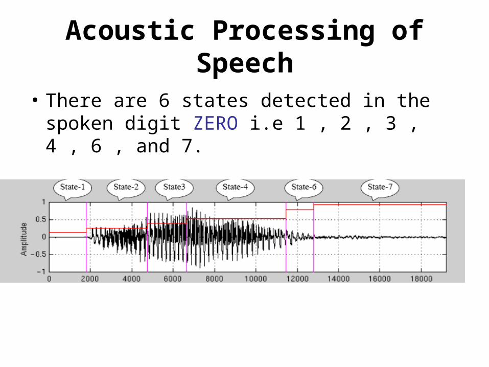
• There are 6 states detected in the spoken digit ZERO i.e 1 , 2 , 3 , 4 , 6 , and 7.

Acoustic Processing of Speech

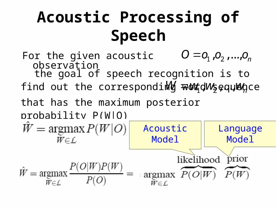
1 2, ,..., nO o o o

1 2, ,..., nW w w w

For the given acoustic observation

the goal of speech recognition is to find out the corresponding word sequence

that has the maximum posterior probability P(W|O)

Acoustic Model Language Model

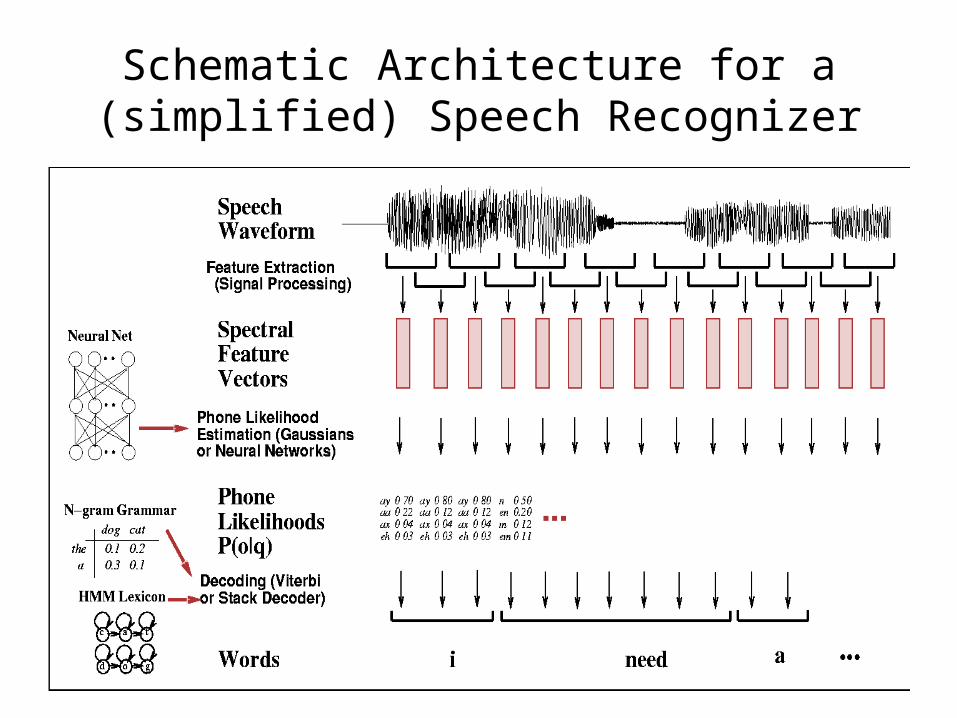
Schematic Architecture for a (simplified) Speech Recognizer

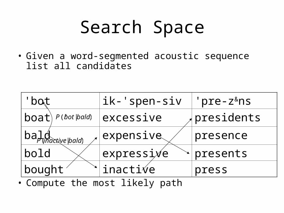
Search Space

• Given a word-segmented acoustic sequence list all candidates

• Compute the most likely path

'bot ik-'spen-siv 'pre-z&ns

boat excessive presidents

bald expensive presence

bold expressive presents

bought inactive press

P(inactive |bald)

P('bot |bald)

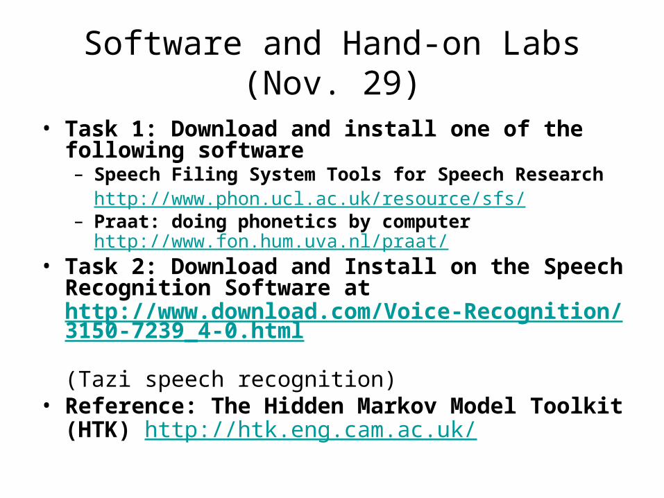
Software and Hand-on Labs (Nov. 29)

• Task 1: Download and install one of the following software– Speech Filing System Tools for Speech Research

http://www.phon.ucl.ac.uk/resource/sfs/ – Praat: doing phonetics by computer

http://www.fon.hum.uva.nl/praat/ • Task 2: Download and Install on the Speech

Recognition Software at http://www.download.com/Voice-Recognition/3150-7239_4-0.html (Tazi speech recognition)

• Reference: The Hidden Markov Model Toolkit (HTK) http://htk.eng.cam.ac.uk/

Introduction to Markov models

Pattern recognition problem:

Need to have good templates that are representative of speech patterns we want to recognize.– How should we model the patterns?– How can we optimize the model’s

parameters?

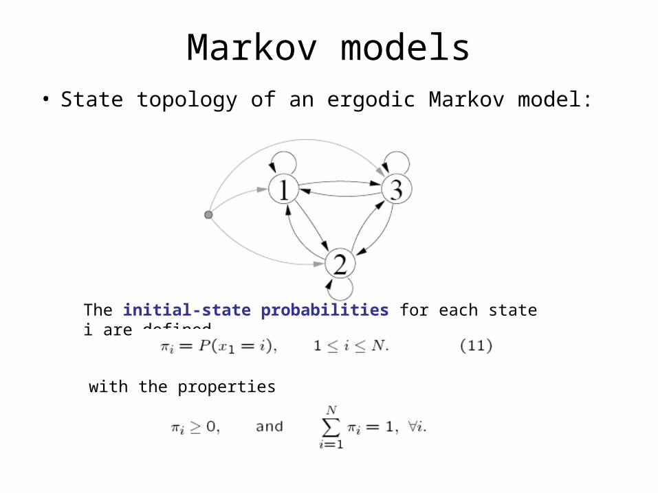
Markov models• State topology of an ergodic Markov model:

The initial-state probabilities for each state i are defined

with the properties

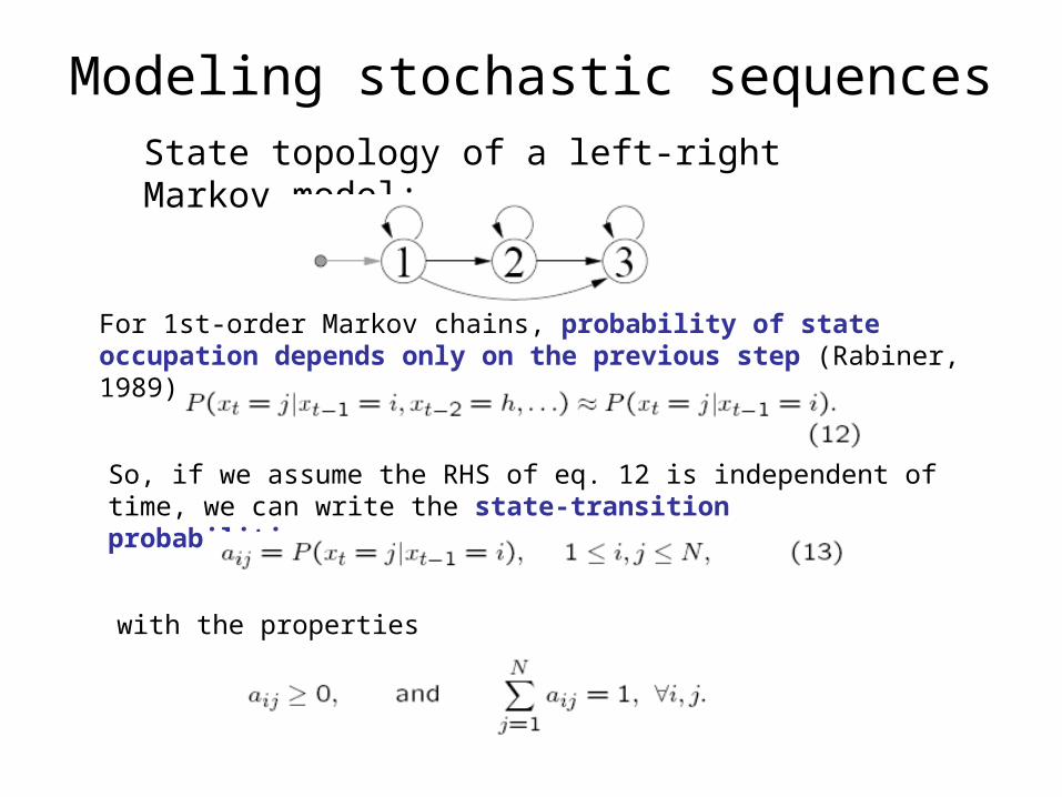
Modeling stochastic sequencesState topology of a left-right Markov model:

For 1st-order Markov chains, probability of state occupation depends only on the previous step (Rabiner, 1989):

So, if we assume the RHS of eq. 12 is independent of time, we can write the state-transition probabilities as

with the properties

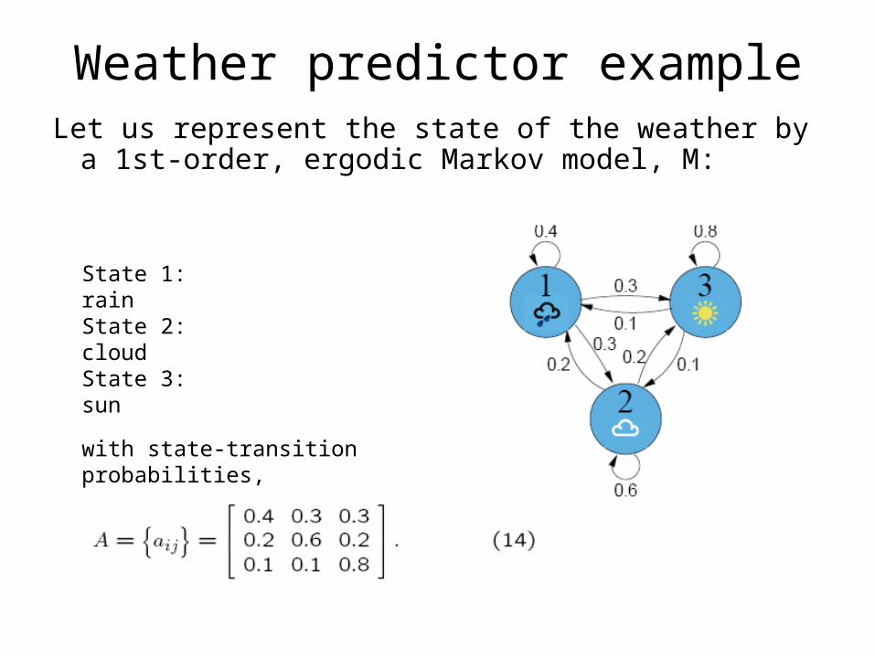
Weather predictor exampleLet us represent the state of the weather by a 1st-

order, ergodic Markov model, M:

State 1: rainState 2: cloudState 3: sun

with state-transition probabilities,

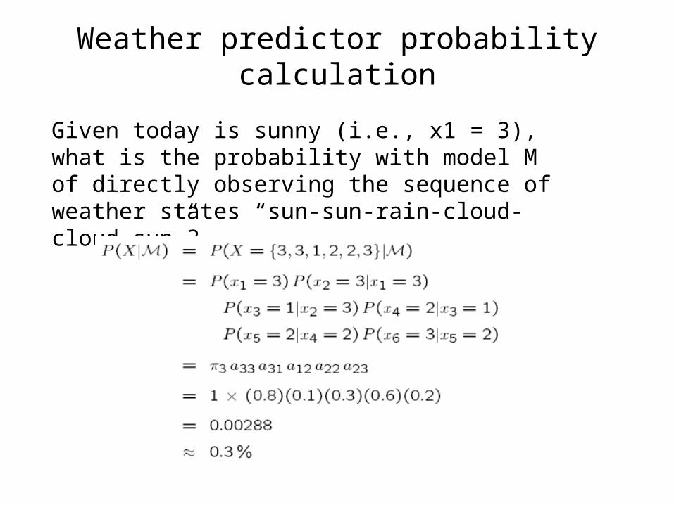
Weather predictor probability calculation

Given today is sunny (i.e., x1 = 3), what is the probability with model M of directly observing the sequence of weather states “sun-sun-rain-cloud-cloud-sun”?

• Formants are the resonant frequencies of the vocal tract when vowels are pronounced.

• Linguists classify each type of speech sound (called phonemes) into different categories. In order to identify each phoneme, it is sometimes useful to look at its spectrogram or frequency response where one can find the characteristic formants.

• Formant values can vary widely from person to person, but the spectrogram reader learns to recognize patterns which are independent of particular frequencies and which identify the various phonemes with a high degree of reliability.

Formants

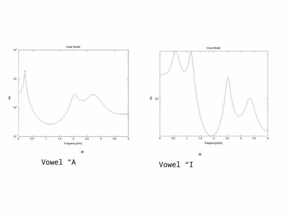
Vowel “I”Vowel “A”

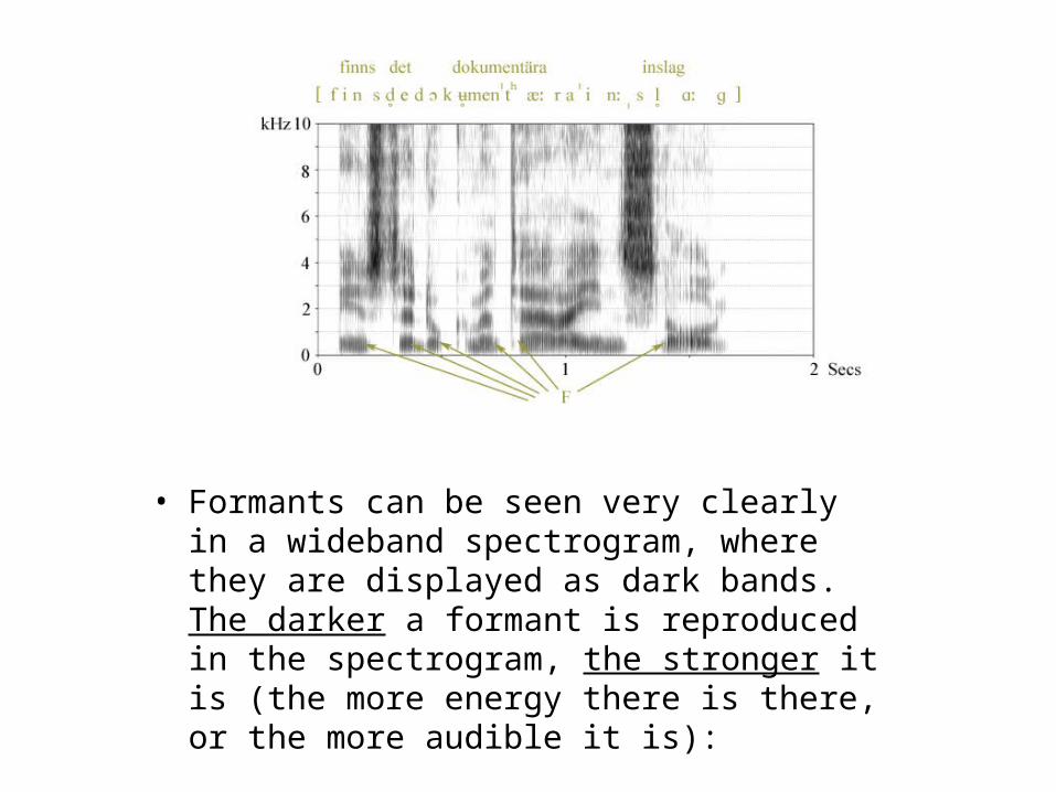
• Formants can be seen very clearly in a wideband spectrogram, where they are displayed as dark bands. The darker a formant is reproduced in the spectrogram, the stronger it is (the more energy there is there, or the more audible it is):

• But there is a difference between oral vowels on one hand, and consonants and nasal vowels on the other.

• Nasal consonants and nasal vowels can exhibit additional formants, nasal formants, arising from resonance within the nasal branch.

• Consequently, nasal vowels may show one or more additional formants due to nasal resonance, while one or more oral formants may be weakened or missing due to nasal antiresonance.

Formants

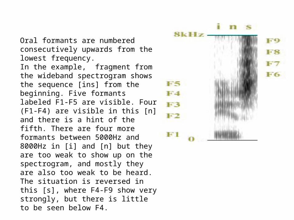
Oral formants are numbered consecutively upwards from the lowest frequency.In the example, fragment from the wideband spectrogram shows the sequence [ins] from the beginning. Five formants labeled F1-F5 are visible. Four (F1-F4) are visible in this [n] and there is a hint of the fifth. There are four more formants between 5000Hz and 8000Hz in [i] and [n] but they are too weak to show up on the spectrogram, and mostly they are also too weak to be heard. The situation is reversed in this [s], where F4-F9 show very strongly, but there is little to be seen below F4.

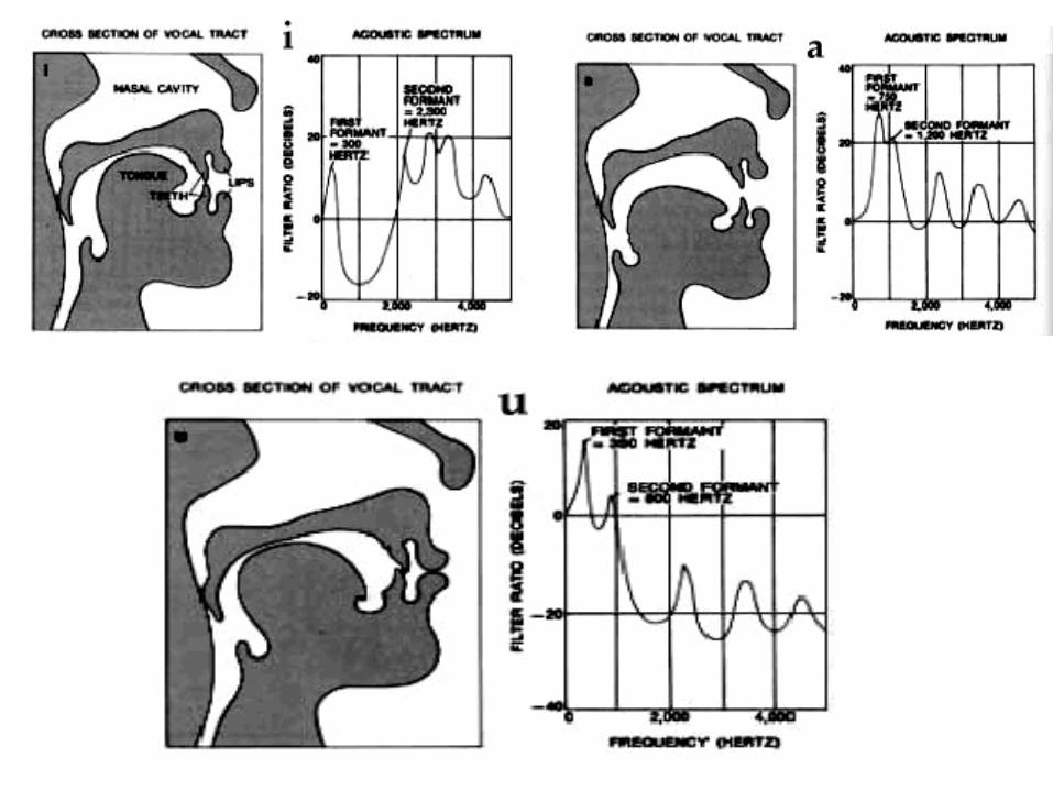
Individual Differences in Vowel Production

• There are differences in individual formant frequencies attributable to size, age, gender, environment, and speech.

• The acoustic differences that allow us to differentiate between various vowel productions are usually explained by a source-filter theory.

• The source is the sound spectrum created by airflow through the glottis which varies as vocal folds vibrate. The filter is the vocal track itself- its shape is controlled by the speaker.

• The three figures below (taken from Miller) illustrate how different configurations of the vocal tract selective pass certain frequencies and not others. The first shows the configuration of the vocal tract while articulating the phoneme [i] as in the word "beet," the second the phoneme [a], as in "father," and the third [u] as in "boot." Note how each configuration uniquely affects the acoustic spectrum--i.e., the frequencies that are passed.