J Dyn Diff Equat (2010) 22:629–655DOI 10.1007/s10884-010-9171-4

Heteroclinic Orbits in Slow–Fast Hamiltonian Systemswith Slow Manifold Bifurcations

Stephen Schecter · Christos Sourdis

Received: 13 April 2009 / Published online: 3 June 2010© Springer Science+Business Media, LLC 2010

Abstract Motivated by a problem in which a heteroclinic orbit represents a moving inter-face between ordered and disordered crystalline states, we consider a class of slow–fastHamiltonian systems in which the slow manifold loses normal hyperbolicity due to a trans-critical or pitchfork bifurcation as a slow variable changes. We show that under assumptionsappropriate to the motivating problem, a singular heteroclinic solution gives rise to a trueheteroclinic solution. In contrast to previous approaches to such problems, our approach usesblow-up of the bifurcation manifold, which allows geometric matching of inner and outersolutions.

Keywords Geometric singular perturbation theory · Blow-up · Pitchfork bifurcation ·Transcritical bifurcation

Mathematics Subject Classification (2000) 34E15 · 34C37 · 37G99

1 Introduction

In [18], the authors consider a multi-order-parameter phase field model developed by Braunet al. [4] for the description of crystalline interphase boundaries. Assuming large anisotropy,a parameter ε is small. The authors are led to consider a second-order system of the form

xττ = gx (x, y), (1.1)

ε2 yττ = gy(x, y); (1.2)

S. Schecter (B)Department of Mathematics, North Carolina State University, Box 8205, Raleigh, NC 27695, USAe-mail: schecter@math.ncsu.edu

C. SourdisDepartamento de Ingeniería Matemática, Universidad de Chile, Casilla 170 Correo 3, Santiago, Chilee-mail: schristos@dim.uchile.cl

123

630 J Dyn Diff Equat (2010) 22:629–655

a heteroclinic orbit of this system that connects certain equilibria represents a moving interfacebetween ordered and disordered states. The system (1.1), (1.2) can be regarded as Hamilto-nian with potential energy −g(x, y); the two equilibria are of course assumed to have equalpotential energy.

The mathematical interest of the problem stems from the fact that, when converted toa 4-dimensional first order system, the 2-dimensional slow manifold undergoes a pitchforkbifurcation along a line as a slow variable changes (and thus is not actually a manifold,although we will refer to it as one). This bifurcation results in loss of normal hyperbolicityof the slow manifold along the line. The limiting problem has a heteroclinic solution thatconnects equilibria on the slow manifold, but it passes through the bifurcation line and infact has a corner there due to the pitchfork bifurcation. The question is whether, for smallε > 0, there is a true heteroclinic solution near this singular solution.

This question has been resolved in the affirmative by Fife [10], who used a shootingargument, and by the authors of [18] based on the contraction mapping principle. Key to theanalysis of [18] is an inner solution, used near the bifurcation point. The existence of theinner solution, which is a solution with appropriate limiting behavior at ±∞ of a nonauton-omous second-order ODE, had already been shown in [1]. The paper [18] is mostly devotedto matching of the inner and outer solutions.

In this paper we consider from the viewpoint of geometric singular perturbation theory[9,13,14] a class of problems that includes the one studied in [18]. In problems involving lossof normal hyperbolicity of the slow manifold, geometric singular perturbation theory typi-cally does not help to find and study the inner solution, but it often does simplify matching ofinner and outer solutions. Matching becomes a geometric problem of identifying the behaviorof certain manifolds of solutions, which can often be resolved using standard results.

Using the blow-up procedure for dealing with loss of normal hyperbolicity of the slowmanifold [8,15], we blow up the bifurcation line to a 3-sphere crossed with a line. The innersolution corresponds to a solution of the blown-up system that connects two equilibria on oneof these spheres. Within the sphere, one equilibrium has a two-dimensional center-unstablemanifold, and the other has a two-dimensional center-stable manifold. Results in [1] on thelinearization of the nonautonomous second-order ODE along the inner solution imply thatthese manifolds intersect transversally along the inner solution. We show that this impliesthat for small ε > 0, the 2-dimensional unstable and stable manifolds of the equilibria tobe connected meet transversally within a 3-dimensional energy surface. This result yieldsexistence of the desired heteroclinic solution.

We begin in Sects. 2 and 3 by describing a slightly simplified version of the system stud-ied in [18]. Then in Sect. 4 we describe a more general version of this system, in which the2-dimensional slow manifold undergoes a pitchfork bifurcation along a line as a slow variablechanges; we give assumptions and state our result. The result is proved in Sects. 5 to 9. InSect. 10 we state the analogous result for transcritical bifurcation of the slow manifold, andindicate where changes in the proof are required.

2 Model System

We consider the second-order system (1.1), (1.2), with

g(x, y) = h(x)− 1

2xy2 + 1

4y4. (2.1)

The function h is C2 and will shortly be described more precisely.

123

J Dyn Diff Equat (2010) 22:629–655 631

Write (1.1), (1.2) as a first-order system (the slow system):

u1τ = u2, (2.2)

u2τ = gx (u1, u3) = h′(u1)− 1

2u2

3, (2.3)

εu3τ = u4, (2.4)

εu4τ = gy(u1, u3) = u33 − u1u3. (2.5)

In (2.2)–(2.5) let τ = εσ . We obtain the fast system:

u1σ = εu2, (2.6)

u2σ = εgx (u1, u3) = ε

(h′(u1)− 1

2u2

3

), (2.7)

u3σ = u4, (2.8)

u4σ = gy(u1, u3) = u33 − u1u3. (2.9)

For each ε, (2.6)–(2.9) has the first integral

H(u1, u2, u3, u4) = 1

2u2

2 + 1

2u2

4 − g(u1, u3).

Indeed, for ε > 0, (2.6)–(2.9) is a Hamiltonian system, with Hamiltonian H , in the sensethat there is a nonsingular skew-symmetric matrix

J =

⎛⎜⎜⎝

0 ε 0 0−ε 0 0 00 0 0 10 0 −1 0

⎞⎟⎟⎠

such that (u1σ u2σ u3σ u4σ )� = J

(∂H∂u1

∂H∂u2

∂H∂u3

∂H∂u4

)�.

The equilibria of (2.6)–(2.9) for ε > 0 are:

• (u1, 0, 0, 0) with h′(u1) = 0.• (u1, 0, u3, 0) with u1 = u2

3 and h′(u1)− 12 u1 = 0.

We make the following assumptions on h. Let

�(x) ={

h′(x) if x ≤ 0,h′(x)− 1

2 x if x > 0.

Then we assume:

(1) There are exactly three points x−, x0, x+, with x− < 0 < x0 < x+, at which �(x) = 0.(2) �′(x−) = h′′(x−) > 0.(3) �′(x0) = h′′(x0)− 1

2 < 0.(4) �′(x+) = h′′(x+)− 1

2 > 0.(5)

∫ x+x− �(x) dx = 0.

(6) h(x−) = 0.

See Fig. 1.With these assumptions the equilibria of (2.6)–(2.9) for ε > 0 are

(x−, 0, 0, 0),

(x0, 0,± x

120 , 0

),

(x+, 0,± x

12+, 0

),

123

632 J Dyn Diff Equat (2010) 22:629–655

Fig. 1 Graph of z = h′(x). Theshaded areas are equal

x− x+x0

x

z z=h’(x)

z=x/2

and possibly others with u2 = u3 = u4 = 0 and u1 > 0.Our goal is to show that for small ε > 0, there is a heteroclinic solution of (2.6)–(2.9) from

(x−, 0, 0, 0) to

(x+, 0, x

12+, 0

). There is another from (x−, 0, 0, 0) to

(x+, 0,−x

12+, 0

), but

we shall not consider it.

Lemma 2.1 h(x+) = 14 x2+.

Proof

0 =x+∫

x−

�(x)dx =0∫

x−

h′(x)dx +x+∫

0

(h′(x)− 1

2x

)dx

= h(0)+(

h(x+)− 1

4x2+ − h(0)

)= h(x+)− 1

4x2+. ��

Using assumption (6) and Lemma 2.1, we see that

H(x−, 0, 0, 0) = H

(x+, 0, x

12+, 0

)= 0.

It is easy to check that for ε > 0, (x−, 0, 0, 0) and

(x+, 0, x

12+, 0

)are hyperbolic equilibria

of (2.6)–(2.9) with two negative eigenvalues and two positive eigenvalues. The heteroclin-ic solution that we will find corresponds to an intersection of the 2-dimensional manifolds

W uε (x−, 0, 0, 0) and W s

ε

(x+, 0, x

12+, 0

)that is transverse within the 3-dimensional manifold

H−1(0) (which is indeed a manifold away from equilibria).

3 Fast Limit and Slow Systems

Setting ε = 0 in (2.6)–(2.9), we obtain the fast limit system:

u1σ = 0, (3.1)

u2σ = 0, (3.2)

u3σ = u4, (3.3)

u4σ = gy(u1, u3) = −u1u3 + u33. (3.4)

123

J Dyn Diff Equat (2010) 22:629–655 633

The equilibria of (3.1)–(3.4) are the 2-dimensional plane

E = {(u1, u2, 0, 0) : u1 and u2 arbitrary}and the 2-dimensional parabolic cylinder

F = {(u1, u2, u3, 0) : u1 = u23, u2 and u3 arbitrary}.

These two surfaces meet along the u2-axis. See Fig. 3.The matrix of the linearization of (3.1)–(3.4) is⎛

⎜⎜⎝0 0 0 00 0 0 00 0 0 1

gxy(u1, u3) 0 gyy(u1, u3) 0

⎞⎟⎟⎠ =

⎛⎜⎜⎝

0 0 0 00 0 0 00 0 0 1

−u3 0 −u1 + 3u23 0

⎞⎟⎟⎠ . (3.5)

Therefore equilibria (u1, u2, u3, u4) of (3.1)–(3.4) are normally hyperbolic if and only ifgyy(u1, u3) = −u1 + 3u2

3 > 0, in which case there is one positive and one negative eigen-value, in addition to two zero eigenvalues. Hence (3.1)–(3.4) has three manifolds of normallyhyperbolic equilibria:

E− = {(u1, u2, 0, 0) : u1 < 0 and u2 arbitrary} ,F− =

{(u1, u2,−u

121 , 0

): u1 > 0 and u2 arbitrary

},

F+ ={(

u1, u2, u121 , 0

): u1 > 0 and u2 arbitrary

}.

In addition, there is a manifold of equilibria E+ = {(u1, u2, 0, 0) : u1 > 0 and u2 arbitrary}that is not normally hyperbolic. See Fig. 3.

Setting ε = 0 in (2.2)–(2.5), we obtain the slow limit system:

u1τ = u2, (3.6)

u2τ = gx (u1, u3) = −1

2u2

3 + h′(u1), (3.7)

0 = u4, (3.8)

0 = gy(u1, u3) = −u1u3 + u33. (3.9)

E−, E+, F−, and F+ are manifolds of solutions of the algebraic Eqs. 3.8, 3.9. Equations 3.6,3.7 then give the slow system on these manifolds. We are interested only in the slow systemon E− and F+.

Slow system on E− (u1 < 0, u2 arbitrary):

u1τ = u2, (3.10)

u2τ = gx (u1, 0) = h′(u1). (3.11)

Slow system on F+ (u1 > 0, u2 arbitrary):

u1τ = u2, (3.12)

u2τ = gx

(u1, u

121

)= −1

2u1 + h′(u1). (3.13)

Phase portraits of (3.10), (3.11) and (3.12), (3.13), both extended to u1 = 0, are shown inFig. 2. Note:

123

634 J Dyn Diff Equat (2010) 22:629–655

u2 u2

u1

u2*u2

*

x+x0x−

(a) (b)

Fig. 2 a Phase portrait of (3.10)–(3.11), u1 ≤ 0. b Phase portrait of (3.12)–(3.13), u1 ≥ 0

Fig. 3 Phase portrait of the slowlimit system (3.6)–(3.9) on E−and F+. The space u4 = 0 isshown

x−u1

u2

u3

E−

F+

Γ−

Γ+

u2*

F−

E+

(1) For (3.10), (3.11), (x−, 0) is a hyperbolic saddle, and a branch of its unstable manifoldmeets the u2 axis at a point (0, u∗

2).(2) For (3.12), (3.13), (x+, 0) is a hyperbolic saddle, and a branch of its stable manifold

meets the u2 axis at the same point (0, u∗2).

We must have 0 = H(0, u∗2, 0, 0) = 1

2 (u∗2)

2 − h(0), so u∗2 = (2h(0))

12 .

Figure 3 shows the phase portrait of the slow limit system (3.6)–(3.9) on E− and F+. Let

• �− denote the set of (u1, u2, 0, 0) such that x− < u1 < 0 and (u1, u2) is in the unstablemanifold of (x−, 0) for (3.10), (3.11);

• �+ denote the set of

(u1, u2, u

121 , 0

)such that 0 < u1 < x+ and (u1, u2) is in the stable

manifold of (x+, 0) for (3.12), (3.13).

The following result is proved in [10] and [18]:

123

J Dyn Diff Equat (2010) 22:629–655 635

Theorem 3.1 For small ε > 0, there is a heteroclinic solution of (2.6)–(2.9) from (x−, 0, 0, 0)

to

(x+, 0, x

12+, 0

)that is close to �− ∪ {(0, u∗

2, 0, 0)} ∪ �+.

In the following sections we shall prove a somewhat more general result.

4 General System

We consider the system

xτ τ = gx (x, y, ε), (4.1)

ε2 yτ τ = gy(x, y, ε), (4.2)

where g is smooth and

g(x, y, ε) = h(x, ε)+ yk(x, y, ε). (4.3)

We assume:

(P1) At (x, y, ε) = (0, 0, 0), k = kx = k y = kε = k y y = 0, kx y < 0, k y y y > 0. (4.4)

Hence

k(x, y, 0) = λx2 − μ

2x y + ν

4y3 + · · · (4.5)

with λ arbitrary,μ > 0, and ν > 0; “…” represents other cubic terms and higher order terms.A simple change of variables allows us to assume μ = ν = 1. More precisely, the change

of variables

x = μ

νx, y = μ

νy, τ = ν

12

μτ

converts (4.1), (4.2) to

xττ = gx (x, y, ε), (4.6)

ε2 yττ = gy(x, y, ε), (4.7)

withg(x, y, ε) = h(x, ε)+ yk(x, y, ε),

where g(x, y, ε) = ν3

μ4 g(μν

x, μν

y, ε), h(x, ε) = ν3

μ4 h(μν

x, ε), and k(x, y, ε) =

ν2

μ3 k(μν

x, μν

y, ε); hence

k(x, y, 0) = ωx2 − 1

2xy + 1

4y3 + · · · ,

withω = λμ

; “…” represents other cubic terms and higher order terms. For the model system,the rescaling is not necessary; h is independent of ε and satisfies the assumptions given inSect. 2, and k(x, y, ε) = − 1

2 xy + 14 y3.

We note that

gx (x, y, 0) = hx (x, 0)+ ykx (x, y, 0) = hx (x, 0)+ y

(2ωx − 1

2y + · · ·

), (4.8)

gy(x, y, 0) = k(x, y, 0)+ yky(x, y, 0) = ωx2 − xy + y3 + · · · ; (4.9)

123

636 J Dyn Diff Equat (2010) 22:629–655

in (4.8), “…” represents higher order terms; in (4.9), “…” represents other cubic terms andhigher order terms.

Write (4.6), (4.7) as a first-order system (the slow system):

u1τ = u2, (4.10)

u2τ = gx (u1, u3, ε), (4.11)

εu3τ = u4, (4.12)

εu4τ = gy(u1, u3, ε). (4.13)

In (4.10)–(4.13) let τ = εσ . We obtain the fast system:

u1σ = εu2, (4.14)

u2σ = εgx (u1, u3, ε), (4.15)

u3σ = u4, (4.16)

u4σ = gy(u1, u3, ε). (4.17)

For each ε, (4.14)–(4.17) has the first integral

H(u1, u2, u3, u4) = 1

2u2

2 + 1

2u2

4 − g(u1, u3, ε), (4.18)

and is Hamiltonian in the sense described in Sect. 2.Setting ε = 0 in (4.14)–(4.17), we obtain the fast limit system:

u1σ = 0, (4.19)

u2σ = 0, (4.20)

u3σ = u4, (4.21)

u4σ = gy(u1, u3, 0). (4.22)

There exist ue > 0 and u f > 0 such that this system has two 2-dimensional manifolds ofequilibria (see [11, Ch. 1]), defined as follows:

E = {(u1, u2, u3, 0) : |u1| < ue, u2 arbitrary, u3 = e(u1) = ωu1 + · · · },F = {(u1, u2, u3, 0) : |u3| < u f , u2 arbitrary, u1 = f (u3) = u2

3 + · · · }.E and F meet along the u2-axis. For the model system, we can take ue = u f = ∞; e(u1) = 0and f (u3) = u2

3.The matrix of the linearization of (4.19)–(4.22) is⎛

⎜⎜⎝0 0 0 00 0 0 00 0 0 1

gxy(u1, u3, 0) 0 gyy(u1, u3, 0) 0

⎞⎟⎟⎠ . (4.23)

Therefore equilibria (u1, u2, u3, u4) of (4.19)–(4.22) are normally hyperbolic if and onlyif gyy(u1, u3, 0) > 0, in which case there is one positive and one negative eigenvalue, inaddition to two zero eigenvalues.

We have gyy(x, y, 0) = −x +3y2 +· · ·. Therefore, on E, gyy(u1, e(u1), 0) = −u1 +· · ·,and on F, gyy( f (u3), u3, 0) = −(u2

3 +· · · )+3u23 +· · · = 2u2

3 +· · ·. We define E− (respec-tively E+) to be the subset of E with u1 < 0 (respectively u1 > 0), and F− (respectivelyF+) to be the subset of F with u3 < 0 (respectively u3 > 0). E−, F−, and F+ are normallyhyperbolic for (4.19)–(4.22).

123

J Dyn Diff Equat (2010) 22:629–655 637

The equation u1 = f (u3) can be solved for u3 as a smooth function of w with w2 = u1:u3 = m(w) = w + · · ·. Then there exists um > 0 such that

F− ={(u1, u2, u3, 0) : 0 < u1 < um, u2 arbitrary, and u3 = m

(−u

121

)= −u

121 + · · ·

},

F+ ={(u1, u2, u3, 0) : 0 < u1 < um, u2 arbitrary, and u3 = m

(u

121

)= u

121 + · · ·

}.

For the model system, we can take um = ∞, and m(w) = w, so F− is given by u3 = −u121 ,

and F+ is given by u3 = u121 .

Setting ε = 0 in (4.10)–(4.13), we obtain the slow limit system:

u1τ = u2, (4.24)

u2τ = gx (u1, u3, 0), (4.25)

0 = u4, (4.26)

0 = gy(u1, u3, 0). (4.27)

E−, E+, F−, and F+ are manifolds of solutions of the system of Eqs. 4.26, 4.27. Equa-tions (4.24), (4.25) then give the slow system on these manifolds. We are interested only inthe slow system on E− and F+.

Slow system on E−:

u1τ = u2, (4.28)

u2τ = gx (u1, e(u1), 0), (4.29)

with −ue < u1 < 0 and u2 arbitrary.Slow system on F+:

u1τ = u2, (4.30)

u2τ = gx

(u1,m

(u

121

), 0

), (4.31)

with 0 < u1 < um and u2 arbitrary.We assume:

(P2) The system (4.28), (4.29) has a hyperbolic saddle equilibrium (x−, 0) with −ue <

x− < 0. One branch B− of its unstable manifold arrives at a point (0, u∗2) on the

u2-axis with u∗2 > 0.

(P3) The system (4.30), (4.31) has a hyperbolic saddle equilibrium (x+, 0) with 0 < x+ <um . One branch B+ of its stable manifold arrives at the same point (0, u∗

2) on theu2-axis.

It follows that:

(1) System (4.14)–(4.17) has the smooth families of equilibria p−(ε) and p+(ε), with

p−(0) = (x−, 0, e(x−), 0) and p+(0) =(

x+, 0,m

(x

12+), 0

). For ε > 0 these equi-

libria are hyperbolic, with two eigenvalues with positive real part and two with negativereal part. For the model system p±(ε) are independent of ε.

(2) H(p−(0)) = H(p+(0)).

123

638 J Dyn Diff Equat (2010) 22:629–655

Remark 4.1 Conversely, it is easy to show that (P2) and (P3) follow from (1), (2), if we further

assume that g(x, y, 0) > g(x−, e(x−), 0) on {(x, e(x)), x− < x ≤ 0} ∪ {(

x,m(x12 )

), 0 ≤

x < x+} (see [2]). Note that (x−, e(x−)),(

x+,m

(x

12+))

are equal nondegenerate minima

of g(·, ·, 0).

We assume:

(P4) H(p−(ε)) = H(p+(ε)) for ε ≥ 0.

Let

• �− denote the set of (u1, u2, e(u1), 0) such that (u1, u2) ∈ B−;

• �+ denote the set of

(u1, u2,m

(u

121

), 0

)such that (u1, u2) ∈ B+.

We shall prove

Theorem 4.2 Assume (P1)–(P4). Then for small ε > 0, there is a heteroclinic solution of(4.14)–(4.17) from p−(ε) to p+(ε) that is close to �− ∪ {(0, u∗

2, 0, 0)} ∪ �+.

5 Blow-Up

To the fast system (4.14)–(4.17) we append the equation εσ = 0, obtaining the followingsystem on u1u2u3u4ε-space:

u1σ = εu2, (5.1)

u2σ = εgx (u1, u3, ε), (5.2)

u3σ = u4, (5.3)

u4σ = gy(u1, u3, ε), (5.4)

εσ = 0. (5.5)

In u1u2u3u4ε-space we shall blow up the u2-axis, which consists of equilibria of (5.1)–(5.4) with ε = 0 that are not normally hyperbolic within u1u2u3u4-space, to the product ofu2-space with a 3-sphere. The 3-sphere is a blow-up of the origin in u1u3u4ε-space.

The blowup transformation is a map� from blow-up space R×S3×[0,∞) to u1u2u3u4ε-space defined as follows. Let (u2, (u1, u3, u4, ε), r) be a point of R × S3 × [0,∞); we haveu2

1 + u23 + u2

4 + ε2 = 1. Then the blow-up transformation � is given by

u1 = r2u1, u2 = u2, u3 = r u3, u4 = r2u4, ε = r3ε. (5.6)

Under this transformation the system (5.1)–(5.5) pulls back to a vector field X on blow-upspace for which the blow-up cylinder r = 0 consists entirely of equilibria. The vector fieldwe shall study is X = r−1 X . Division by r desingularizes the vector field on the blow-upcylinder but leaves it invariant.

Note that

�−1(E− × {0}) = �−1{(u1, u2, u3, 0, 0) : −ue < u1 < 0, u2 arbitrary, u3 = e(u1)}is a 2-dimensional submanifold of blowup space. Let E− denote �−1(E− × {0}) togetherwith its limit points in the blow-up cylinder r = 0. We define E+, F−, and F+ analogously.

123

J Dyn Diff Equat (2010) 22:629–655 639

Fig. 4 Blow-up space and thesingular connecting orbit. Notethat the blow-up has separatedthe four manifolds E± and F±

u2

p~−(ε)

p~+(ε)

Γ−Γ+

q−

q+

~

~~

~

Γ0~

E−

F+

F−

E+

~

~

~ ~

Let p−(ε) (respectively p+(ε)) be the unique point in blow-up space that corresponds top−(ε) (respectively p+(ε)); we calculate the coordinates of these points using (5.6). In orderto prove Theorem 3.1, we wish to show that for small ε > 0 there is an integral curve of Xfrom p−(ε) to p+(ε). Equivalently, we shall show that for small ε > 0 there is an integralcurve of X from p−(ε) to p+(ε).

Corresponding to �± are curves �± in blow-up space. We shall see that:

• �− approaches a point q− = (u∗2, q−, 0) on the blow-up cylinder.

• �+ approaches a point q+ = (u∗2, q+, 0) on the blow-up cylinder.

• On the blow-up cylinder, each 3-sphere u2 = constant is invariant.

Proposition 5.1 There is an integral curve �0 of X from q− to q+ that lies in the 3-dimen-sional hemisphere given by u2 = u∗

2, r = 0, ε > 0.

Theorem 5.2 For small ε > 0, there is an integral curve �(ε) of X from p−(ε) to p+(ε).As ε → 0, �(ε) → �− ∪ {q−} ∪ �0 ∪ {q+} ∪ �+.

See Fig. 4. �− and �+ are outer solutions; �0 is the inner solution. The union in Theo-rem 5.2 is the singular solution. Theorem 5.2 implies Theorem 4.2. The next four sectionsare devoted to the proofs of Proposition 5.1 and Theorem 5.2.

6 Charts

We shall need three charts on open subsets of blow-up space.

6.1 Chart for ε > 0

On the set of points in R × S3 × [0,∞) with ε > 0, this chart uses the coordinates b1 =u1ε

− 23 , u2, b3 = u3ε

− 13 , b4 = u4ε

− 23 , and r = r ε

13 . Thus we have

u1 = r2b1, u2 = u2, u3 = rb3, u4 = r2b4, ε = r3, (6.1)

123

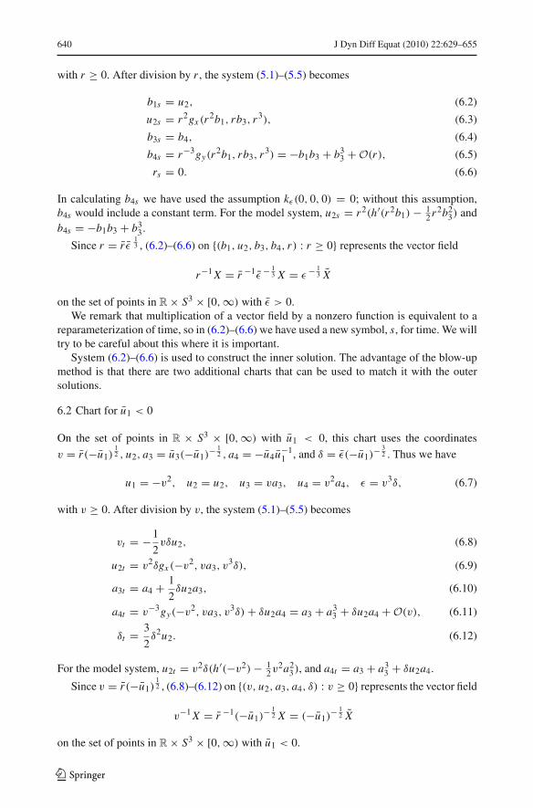
640 J Dyn Diff Equat (2010) 22:629–655

with r ≥ 0. After division by r , the system (5.1)–(5.5) becomes

b1s = u2, (6.2)

u2s = r2gx (r2b1, rb3, r

3), (6.3)

b3s = b4, (6.4)

b4s = r−3gy(r2b1, rb3, r

3) = −b1b3 + b33 + O(r), (6.5)

rs = 0. (6.6)

In calculating b4s we have used the assumption kε(0, 0, 0) = 0; without this assumption,b4s would include a constant term. For the model system, u2s = r2(h′(r2b1)− 1

2r2b23) and

b4s = −b1b3 + b33.

Since r = r ε13 , (6.2)–(6.6) on {(b1, u2, b3, b4, r) : r ≥ 0} represents the vector field

r−1 X = r −1ε − 13 X = ε − 1

3 X

on the set of points in R × S3 × [0,∞) with ε > 0.We remark that multiplication of a vector field by a nonzero function is equivalent to a

reparameterization of time, so in (6.2)–(6.6) we have used a new symbol, s, for time. We willtry to be careful about this where it is important.

System (6.2)–(6.6) is used to construct the inner solution. The advantage of the blow-upmethod is that there are two additional charts that can be used to match it with the outersolutions.

6.2 Chart for u1 < 0

On the set of points in R × S3 × [0,∞) with u1 < 0, this chart uses the coordinates

v = r(−u1)12 , u2, a3 = u3(−u1)

− 12 , a4 = −u4u−1

1 , and δ = ε(−u1)− 3

2 . Thus we have

u1 = −v2, u2 = u2, u3 = va3, u4 = v2a4, ε = v3δ, (6.7)

with v ≥ 0. After division by v, the system (5.1)–(5.5) becomes

vt = −1

2vδu2, (6.8)

u2t = v2δgx (−v2, va3, v3δ), (6.9)

a3t = a4 + 1

2δu2a3, (6.10)

a4t = v−3gy(−v2, va3, v3δ)+ δu2a4 = a3 + a3

3 + δu2a4 + O(v), (6.11)

δt = 3

2δ2u2. (6.12)

For the model system, u2t = v2δ(h′(−v2)− 12v

2a23), and a4t = a3 + a3

3 + δu2a4.

Since v = r(−u1)12 , (6.8)–(6.12) on {(v, u2, a3, a4, δ) : v ≥ 0} represents the vector field

v−1 X = r −1(−u1)− 1

2 X = (−u1)− 1

2 X

on the set of points in R × S3 × [0,∞) with u1 < 0.

123

J Dyn Diff Equat (2010) 22:629–655 641

6.3 Chart for u1 > 0

On the set of points in R × S3 × [0,∞) with u1 > 0, this chart uses the coordinates

w = r u121 , u2, c3 = u3u

− 12

1 , c4 = u4u−11 , and γ = εu

− 32

1 . Thus we have

u1 = w2, u2 = u2, u3 = wc3, u4 = w2c4, ε = w3γ, (6.13)

with w ≥ 0. After division by w, the system (5.1)–(5.5) becomes

wt = 1

2wγ u2, (6.14)

u2t = w2γ gx (w2, wc3, w

3γ ), (6.15)

c3t = c4 − 1

2γ u2c3, (6.16)

c4t = w−3gy(w2, wc3, w

3γ )− γ u2c4 = −c3 + c33 − γ u2c4 + O(w), (6.17)

γt = −3

2γ 2u2. (6.18)

For the model system, u2t = w2γ (h′(w2)− 12w

2c23), and c4t = −c3 + c3

3 − γ u2c4.

Since w = r u12

1 , (6.14)–(6.18) on {(w, u2, c3, c4, γ ) : w ≥ 0} represents the vector field

w−1 X = r −1u− 1

21 X = u

− 12

1 X

on the set of points in R × S3 × [0,∞) with u1 > 0.

6.4 Important Sets and First Integral

1. Note that

�−1{(u1, u2, u3, u4, ε) : ε = 0 and u21 + u2

3 + u24 > 0}

= {(u2, (u1, u3, u4, ε), r) : ε = 0 and r > 0}.It is invariant under X ; hence so is its closure, which is the subset ε = 0 of blow-upspace. In the chart for u1 < 0 (respectively u1 > 0), the corresponding invariant set isδ = 0 (respectively γ = 0).

2. In the chart for u1 < 0, E− corresponds to

E−a ={(v, u2, v

−1e(−v2), 0, 0) : 0 ≤ v < u12e and u2 arbitrary

}

={(v, u2,−ωv + · · · , 0, 0) : 0 ≤ v < u

12e and u2 arbitrary

}.

For the model system, E−a = {(v, u2, 0, 0, 0) : 0 ≤ v}. For the system (6.8)–(6.12),E−a is a 2-dimensional manifold of equilibria that is normally hyperbolic within thespace δ = 0. Note that normal hyperbolicity is not lost at v = 0, which corresponds tou1 = 0.Similarly, in the chart for u1 > 0, E+, F−, and F+ correspond respectively to

• E+c ={(w, u2, w

−1e(w2), 0, 0) : 0 ≤ w < u12e and u2 arbitrary

}

={(w, u2, ωw + · · · , 0, 0) : 0 ≤ w < u

12e and u2 arbitrary

};

123

642 J Dyn Diff Equat (2010) 22:629–655

• F−c ={(w, u2, w

−1m(−w), 0, 0) : 0 ≤ w < u12m and u2 arbitrary

}

={(w, u2,−1 + · · · , 0, 0) : 0 ≤ w < u

12m and u2 arbitrary

};

• F+c ={(w, u2, w

−1m(w), 0, 0) : 0 ≤ w < u12m and u2 arbitrary

}

={(w, u2, 1 + . . . , 0, 0) : 0 ≤ w < u

12m and u2 arbitrary

}.

For the model system, E+c = {(w, u2, 0, 0, 0) : w ≥ 0}, F−c = {(w, u2,−1, 0, 0) :w ≥ 0}, and F+c = {(w, u2, 1, 0, 0) : w ≥ 0}. For the system (6.14)–(6.18), each is a2-dimensional manifold of equilibria. F−c and F+c are normally hyperbolic within thespace γ = 0. Normal hyperbolicity is not lost at w = 0, which corresponds to u1 = 0.

3. In the chart for u1 < 0, p−(ε) corresponds to a unique point p−a(δ), and �− correspondsto

�−a = {(v, u2, a3, 0, 0) : (−v2, u2, va3, 0) ∈ �−}.As v → 0, �−a approaches (0, u∗

2, 0, 0, 0). �− ends at q− = (u∗2, q−, 0), q− =

(−1, 0, 0, 0).In the chart for u1 > 0, p+(ε) corresponds to a unique point p+c(γ ), and �+ correspondsto

�+c = {(w, u2, c3, 0, 0) : (w2, u2, wc3, 0) ∈ �+}.As w → 0, �+c approaches (0, u∗

2, 1, 0, 0). Let α = 12 (5

12 − 1). �+ ends at q+ =

(u∗2, q+, 0), q+ = (α, α

12 , 0, 0).

4. The first integral H for (5.1)–(5.5) becomes:

• In blow-up space: H(u2, (u1, u3, u4, ε), r) = 12 u2

2 + 12 r4u2

4 − g(r2u1, r u3, r3ε).• In the chart for ε > 0: Hb(b1, u2, b3, b4, r) = 1

2 u22 + 1

2r4b24 − g(r2b1, rb3, r3).

• In the chart for u1 < 0: Ha(v, u2, a3, a4, δ) = 12 u2

2 + 12v

4a24 − g(−v2, va3, v

3δ).• In the chart for u1 > 0: Hc(w, u2, c3, c4, γ ) = 1

2 u22 + 1

2w4c2

4 − g(w2, wc3, w3γ ).

H is a first integral for X and hence for X . Hb, Ha , and Hc are first integrals for (6.2)–(6.6),(6.8)–(6.12), and (6.14)–(6.18) respectively. Therefore:

• In blow-up space, each 3-sphere u2 is constant, r = 0 is invariant for X .• In the chart for ε > 0, each space u2 = constant, r = 0 is invariant for (6.2)–(6.6).• In the chart for u1 < 0, each space u2 = constant, v = 0 is invariant for (6.8)–(6.12).• In the chart for u1 > 0, each space u2 = constant, w = 0 is invariant for (6.14)–(6.18).

Of course the last three conclusions also follow easily from inspection of the systems them-selves.

7 Proof of Proposition 5.1

Let X denote the restriction of the vector field X to the invariant 3-sphere M = {u∗2} × S3 ×

{0}, S3 = {(u1, u3, u4, ε) : u21 + u2

3 + u24 + ε2 = 1}. From Sect. 6 we have the following

charts on M .

123

J Dyn Diff Equat (2010) 22:629–655 643

Fig. 5 Phase portraits of a(7.4)–(7.6) and b (7.7)–(7.9).W cu(0, 0, 0) and W cs (1, 0, 0)are shaded

a3

a4

δ

c3

c4

γ

1

(a) (b)

Chart on the open subset of M with ε > 0: b1 = u1ε− 2

3 , b3 = u3ε− 1

3 , b4 = u4ε− 2

3 . In

this chart, the vector field ε − 13 X is

b1s = u∗2, (7.1)

b3s = b4, (7.2)

b4s = −b1b3 + b33. (7.3)

Chart on the open subset of M with u1 < 0: a3 = u3(−u1)− 1

2 , a4 = −u4u−11 , δ =

ε(−u1)− 3

2 . In this chart, the vector field (−u1)− 1

2 X is

a3t = a4 + 1

2δu∗

2a3, (7.4)

a4t = a3 + a33 + δu∗

2a4, (7.5)

δt = 3

2δ2u∗

2. (7.6)

Chart on the open subset of M with u1 > 0: c3 = u3u− 1

21 , c4 = u4u−1

1 , γ = εu− 3

21 . In

this chart, the vector field u− 1

21 X is

c3t = c4 − 1

2γ u∗

2c3, (7.7)

c4t = −c3 + c33 − γ u∗

2c4, (7.8)

γt = −3

2γ 2u∗

2. (7.9)

The system (7.4)–(7.6) has an equilibrium at the origin with 2-dimensional center-unsta-ble manifold. Abusing notation a little, we let W cu(0, 0, 0) denote the part of this manifoldwith δ ≥ 0. Then W cu(0, 0, 0) consists of all solutions of (7.4)–(7.6) that approach (0, 0, 0)as t → −∞. See Fig. 5a.

The system (7.7)–(7.9) has equilibria at (−1, 0, 0), (0, 0, 0), and (1, 0, 0). The equilib-rium at (1, 0, 0) has a 2-dimensional center-stable manifold. Continuing to abuse notation,we let W cs(1, 0, 0) denote the part of this manifold with γ ≥ 0. Then W cs(1, 0, 0) consistsof all solutions of (7.7)–(7.9) that approach (1, 0, 0) as t → ∞. See Fig. 5b.

Let W cu(q−) and W cs(q+) denote the corresponding manifolds in M , extended to beinvariant. W cu(q−) (respectively W cs(q+)) consists of all integral curves of X that approach

123

644 J Dyn Diff Equat (2010) 22:629–655

q− (respectively q+) as ξ → −∞ (respectively ξ → ∞). To prove Proposition 5.1 we willfind an integral curve of X in W cu(q−) ∩ W cs(q+).

The solution of (7.1) with b1(0) = 0 is b1 = u∗2s. Substituting into (7.3) and combining

(7.2) and (7.3) into a second-order equation, we obtain

b3ss = −u∗2sb3 + b3

3. (7.10)

By [1,18], [3, p. 100], (7.10) has a solution b3(s) with b3s > 0 such that

(S1) b3(s) = O(

|s|− 14 e− 2

3 (u∗2)

12 |s| 3

2

)as s → −∞,

(S2) b3(s) = (u∗2s)

12 + O(s− 5

2 ) as s → ∞,

(S3) b3s(s) ≤ C |s|− 12 , s �= 0.

(u∗2s, b3(s), b3s(s)) is a solution of (7.1)–(7.3). We claim that it represents an intersection of

W cu(q−) and W cs(q+) in the portion of M with ε > 0.The change of coordinates between the chart for ε > 0 and the chart for u1 < 0 is

a3 = b3(−b1)− 1

2 , a4 = −b4b−11 , δ = (−b1)

− 32 .

Using (S1), (S3), and b1 = u∗2s, we see:

(a3(s), a4(s), δ(s)) → (0, 0, 0) as s → −∞. (7.11)

The change of coordinates between the chart for ε > 0 and the chart for u1 > 0 is

c3 = b3(b1)− 1

2 , c4 = b4b−11 , γ = (b1)

− 32 . (7.12)

Using (S2), (S3), and b1 = u∗2s, we see:

(c3(s), c4(s), γ (s)) → (1, 0, 0) as s → ∞. (7.13)

Equations (7.11) and (7.13) yield the result.

Remark 7.1 (a3(s), a4(s), δ(s)) is not a solution of (7.4)–(7.6): it is an integral curve of

ε − 13 X in (a3, a4, δ) coordinates, whereas solutions of (7.4)–(7.6) represent integral curves

of (−u1)− 1

2 X . However, the reparameterization of time t = − 23 (u

∗2)

12 (−s)

32 converts

(a3(s), a4(s), δ(s)), s < 0, to a solution of (7.4)–(7.6), which we denote (a3(t), a4(t), δ(t)).Similarly, the reparameterization of time t = 2

3 (u∗2)

12 s

32 converts (c3(s), c4(s), γ (s)), s >

0, to a solution of (7.7)–(7.9), which we denote (c3(t), c4(t), δ(t)).

Remark 7.2 Using (S1), (S2), and the previous remark, one can show that a3(t) is O(|t |− 12 et )

as t → −∞, but c3(t) − 1 is only O(t−2) as t → ∞. The reason for the difference can beseen in Fig. 5: in the chart on M for u1 < 0, a center manifold for the origin is the δ-axis;in the chart on M for u1 > 0, center manifolds of (1, 0, 0) are skew curves. Since solutionsin W cu(0, 0, 0) approach the center manifold exponentially as t → −∞, and the eigenvalueis 1, we see that a3(t) (and a4(t)) should be O(et ) as t → −∞. No such conclusion can bedrawn about c3(t) and c4(t).

8 Transversality

Let �0 = {(u1, u3, u4, ε) : (u∗2, (u1, u3, u4, ε), 0) ∈ �0}, where �0 is given by Proposi-

tion 5.1.

123

J Dyn Diff Equat (2010) 22:629–655 645

Proposition 8.1 W cu(q−) and W cs(q+) intersect transversally within M along �0.

Note that W cu(q−) and W cs(q+) have dimension 2 and M has dimension 3, so a transverseintersection is 1-dimensional, in this case �0.

Proof The equilibrium (0, 0, 0) of (7.4)–(7.6) has one negative eigenvalue, one positiveeigenvalue, and one zero eigenvalue, and the vector field is quadratic on the center man-ifold. It follows that solutions (a3(t), a4(t), δ(t)) that approach (0, 0, 0) as t → −∞ areO(|t |−1), and solutions of the linearized system along (a3(t), a4(t), δ(t)) that do not growexponentially as t → −∞ are O(t−2). There is a 2-dimensional space of such solutions ofthe linearized system, which we denote Ecu

a (t).Similarly, the equilibrium (1, 0, 0) of (7.7)–(7.9) has one negative eigenvalue, one positive

eigenvalue, and one zero eigenvalue, and the vector field is quadratic on the center manifold.It follows that solutions (c3(t), c4(t), γ (t)) that approach (1, 0, 0) as t → ∞ are O(t−1), andsolutions of the linearized system along (c3(t), c4(t), γ (t)) that do not grow exponentiallyas t → ∞ are O(t−2). There is a 2-dimensional space of such solutions of the linearizedsystem, which we denote Ecs

c (t).Each of these spaces corresponds to a space of solutions of the linearization of X along

�0. More precisely, if �0 is the set of points in the solution y(ξ) of yξ = X(y) on M , thenthe linearized equation Yξ = DX(y(ξ))Y has a 2-dimensional space of solutions Ecu(ξ)

(respectively Ecs(ξ)) consisting of vectors tangent to W cu(q−) (respectively W cs(q+)) aty(ξ). These spaces correspond respectively to Ecu

a (t) in the chart for u1 < 0 and to Ecsc (t) in

the chart for u1 > 0. To prove the result we must show that Ecu(ξ)∩ Ecs(ξ) is 1-dimensional(multiples of yξ (ξ)).

In the chart on M for u1 > 0, �0 corresponds to a solution (c3(t), c4(t), γ (t)) of (7.7)–(7.9). After a shift in time, we may assume γ (t) = 2

3u∗2 t . The linearization of (7.7)–(7.9)

along this solution is⎛⎝ C3t

C4t

�t

⎞⎠ =

⎛⎝ − 1

2 u∗2γ (t) 1 − 1

2 u∗2c3(t)

3c3(t)2 − 1 −u∗2γ (t) −u∗

2c4(t)0 0 −3u∗

2γ (t)

⎞⎠

⎛⎝ C3

C4

�

⎞⎠ . (8.1)

The inverse of the coordinate change (7.12) is

b1 = γ− 23 , b3 = γ− 1

3 c3, b4 = γ− 23 c4. (8.2)

Under this coordinate change, (7.7)–(7.9) becomes

b1t = u∗2b

− 12

1 , (8.3)

b3t = b− 1

21 b4, (8.4)

b4t = b− 1

21 (b3

3 − b1b3). (8.5)

This system is just b− 1

21 times (7.1)–(7.3). Applying (8.2) to (c3(t), c4(t), γ (t)) yields a

solution (b1(t), b3(t), b4(t)) of (8.3)–(8.5) with b1(t) = ( 32 u∗

2t) 2

3 . The linearization of (8.2)along (c3(t), c4(t), γ (t)), which is

⎛⎝ B1

B3

B4

⎞⎠ =

⎛⎜⎝

0 0 − 23γ (t)

− 53

γ (t)− 13 0 − 1

3γ (t)− 4

3 c3(t)

0 γ (t)− 23 − 2

3γ (t)− 5

3 c4(t)

⎞⎟⎠

⎛⎝ C3

C4

�

⎞⎠ , (8.6)

123

646 J Dyn Diff Equat (2010) 22:629–655

converts (8.1) into the linearization of (8.3)–(8.5) along (b1(t), b3(t), b4(t)), namely

⎛⎝B1t

B3tB4t

⎞⎠ =

⎛⎜⎜⎝

− 12 u∗

2b1(t)− 3

2 0 0

− 12 b1(t)

− 32 b4(t) 0 b1(t)

− 12

− 12 b1(t)

− 12 b3(t)− 1

2 b1(t)− 3

2 b3(t)3 b1(t)

− 12 (3b3(t)

2 − b1) 0

⎞⎟⎟⎠

⎛⎝ B1

B3B4

⎞⎠ .

(8.7)

The change of coordinates (8.6) converts Ecsc (t) into a 2-dimensional space of solutions of

(8.7) that we denote Ecsb (t).

One solution of (8.7) is (B1(t), B3(t), B4(t)) = (b1t (t), b3t (t), b4t (t)); it lies in Ecsb (t).

There is a complementary 2-dimensional space of solutions of (8.7) with B1(t) = 0 and(B3, B4)(t) a solution of

(B3t

B4t

)=

(0 b1(t)−

12

b1(t)−12 (3b3(t)2 − b1) 0

) (B3

B4

). (8.8)

If Ecu(ξ) ∩ Ecs(ξ) is not 1-dimensional, then Ecu(ξ) = Ecs(ξ) and corresponds, in thechart for ε > 0, to Ecs

b (t). Since two 2-dimensional spaces in a 3-dimensional space havenontrivial intersection, Ecs

b (t) includes solutions with B1(t) = 0.If (C3(t),C4(t), �(t)) ∈ Ecs

c (t), then C3(t),C4(t), and �(t) are O(t−2). Also,c3(t) is O(1), and c4(t) and γ (t) are O(t−1). Therefore we see from (8.6) that if

(B1(t), B3(t), B4(t)) ∈ Ecsb (t), then B1(t) is O

(t− 1

3

), B3(t) is O

(t− 2

3

), and B4(t) is

O(

t− 43

).

The rescaling of time t = 23 (u

∗2)

12 s

32 converts (8.3)–(8.5) to (7.1)–(7.3), for which b1 =

u∗2s, and converts (8.8) to(

B3s

B4s

)=

(0 1

3b3(s)2 − u∗2s 0

) (B3

B4

). (8.9)

Thus a solution (0, B3(t), B4(t)) of (8.7) in Ecsb (t) becomes (0, B3(s), B4(s)) with

(B3(s), B4(s)) a solution of (8.9); moreover, B3(s) is O(s−1) and B4(s) is O(s−2).A similar argument in the coordinate system for u1 < 0 leads to the following conclusion:

• W cu(q−) and W cs(q+) intersect transversally along �0 if and only if (8.9) has no non-trivial solution (B3(s), B4(s)) on R such that B3 is O(|s|−1), and B4 is O(s−2).

Now (8.9) is equivalent to the second order linear system

B3ss = (3b3(s)2 − u∗

2s)B3. (8.10)

By [1, Theorem 2], (8.10) has no nontrivial solutions in L2, hence no solution for whichB3(s) is O(|s|−1). This completes the proof. ��Remark 8.2 Using Remark 7.2, one can obtain better estimates for (B3(s), B4(s)) as s →−∞, but they are not needed.

9 Proof of Theorem 5.2

Let Nε denote the set of points in blow-up space at which H = H(p−(ε)) and r3ε = ε.Away from equilibria of X , each Nε is a manifold of dimension 3.

123

J Dyn Diff Equat (2010) 22:629–655 647

For the vector field X and ε > 0, the equilibria p−(ε) and p+(ε) have 2-dimensionalunstable and stable manifolds. We will prove the theorem by showing that for small ε >0,W u( p−(ε)) and W s( p+(ε)) have a nonempty intersection that is transverse within Nε . Itwill be clear that the intersection approaches �− ∪ �0 ∪ �+ as ε → 0.

In the chart on blow-up space for u1 < 0, the system (6.8)–(6.12) has the 2-dimensionalmanifold of equilibria E−a . The linearization of (6.8)–(6.12) at a point y of E−a , taking intoaccount that va3 = u3 = O(u1) = O(v2), so that a3 = O(v), and that a4 = δ = 0, has theform ⎛

⎜⎜⎜⎜⎝

0 0 0 0 O(v)0 0 0 0 O(v2)

0 0 0 1 O(v)∗ 0 v−2gyy(−v2, va3, 0) 0 gyε(−v2, va3, 0)0 0 0 0 0

⎞⎟⎟⎟⎟⎠ .

The eigenvalues are±v−1(gyy(−v2, va3, 0))12 = ±(1+3a2

3)12 +· · ·with multiplicity one and

0 with multiplicity three. The eigenvectors for ±v−1(gyy(−v2, va3, 0))12 span a3a4-space, so

the generalized eigenspace Va(y) for the 0 eigenvalues is complementary to a3a4-space. From[7] we deduce that given any compact subset K of E−a , there are a 3-dimensional normallyhyperbolic invariant manifold S− and a number δ0 > 0 such that K ⊂ S−, Ty S− = Va(y)for all y ∈ K , and S− is a smooth graph over {(v, u2, δ) : (v, u2, v

−1e(−v2), 0, 0) ∈K and |δ| < δ0}. For the model system, S− ⊂ vu2δ-space. In the usual fibration of W u(S−),each point of S− has a 1-dimensional unstable fiber.

The equations for S− have the form

a3 = v−1e(−v2)+ O(δ), a4 = O(δ).

Substituting these expressions into (6.8), (6.9), (6.12), we obtain the restriction of (6.8)–(6.12) to S−. Once the system is restricted to S−, each equation has a factor of δ, so we candivide by δ, obtaining

vt = −1

2vu2, (9.1)

u2t = v2gx (−v2, e(−v2)+ O(vδ), v3δ), (9.2)

δt = 3

2δu2. (9.3)

Note that on the invariant plane δ = 0, (9.1), (9.2) with v > 0 is just (4.28), (4.29) withu1 < 0 after making the change of coordinates u1 = −v2 and dividing by v2.

We shall use a ˘ to designate objects related to (9.1)–(9.3). From assumption (P2), (9.1)–

(9.3) has a curve of equilibria p−a(δ), with p−a(δ) = (v, u2, δ), v = (−x−)12 + O(δ), u2 =

0; this curve consists of equilibria that are normally hyperbolic for (9.1)–(9.3), with onepositive eigenvalue and one negative eigenvalue. Of course, the coordinates of p−a(δ) arejust the vu2δ-coordinates of p−a(δ). Note that p−a(δ) ∈ S−. Also, the line {(v, u2, δ) : v =δ = 0, u2 �= 0} consists of equilibria; by direct calculation, they are also normally hyperbolicfor (9.1)–(9.3), with one positive eigenvalue and one negative eigenvalue. See Fig. 6.

Let �−a = {(v, u2, 0) : (v, u2, v−1e(−v2), 0, 0) ∈ �−a}. �−a is a branch of the unsta-

ble manifold of p−a(0) for (9.1)–(9.3), which we denote W u( p−a(0)). It coincides with abranch of the stable manifold of (0, u∗

2, 0) for (9.1)–(9.3), which we denote W s(0, u∗2, 0).

W u(0, u∗2, 0) is just the line {(v, u2, δ) : v = 0, u2 = u∗

2}.

123

648 J Dyn Diff Equat (2010) 22:629–655

Fig. 6 Phase portrait of(9.1)–(9.3)

u2*

u2

v

δ

(−x−)1/2

−aΓ

Lemma 9.1 Consider the system (9.1)–(9.3). For ρ > 0 and k ≥ 2, let Uk = {(v, u2, δ) :|v| < ρ, |u2 − u∗

2| < ρ,ρk < δ < ρ}. If ρ is sufficiently small, then for each k ≥ 2, as

δ0 → 0+, W u( p−a(δ0)) ∩ Uk approaches W u(0, u∗2, 0) ∩ Uk in the C1 topology.

Proof This is a very simple case of the Corner Lemma in [17]. The statement here is a littledifferent, but the same proof applies. ��

With considerable abuse of notation, we let W cu(0, u∗2, 0, 0, 0) denote the set of points

in vu2a3a4δ-space through which the solution of (6.8)–(6.12) approaches (0, u∗2, 0, 0, 0) as

t → −∞. W cu(0, u∗2, 0, 0, 0) is just {(0, u∗

2, a3, a4, δ) : (a3, a4, δ) ∈ W cu(0, 0, 0)}, whereW cu(0, 0, 0) was defined in Sect. 7. Recall that W cu(0, 0, 0) is just W cu(q−) in the chart onM for u1 < 0; similarly, W cu(0, u∗

2, 0, 0, 0) is just W cu(q−) in the chart on blow-up spacefor u1 < 0.

Alternatively, W cu(0, u∗2, 0, 0, 0) is just the union of the unstable fibers of points in the

line v = 0, u2 = u∗2, δ ≥ 0; this line is part of the normally hyperbolic invariant manifold

S−. Therefore Lemma 9.1 implies:

Lemma 9.2 Consider the system (6.8)–(6.12). For ρ > 0 and k ≥ 2, let Uka ={(v, u2, a3, a4, δ) : |v| < ρ, |u2 − u∗

2| < ρ, |a3| < ρ, |a4| < ρ,ρk < δ < ρ. If ρ is

sufficiently small, then for each k ≥ 2, as δ0 → 0+,W u(p−a(δ0)) ∩ Uka approachesW cu(0, u∗

2, 0, 0, 0) ∩ Uka in the C1 topology.

In the chart on blow-up space for u1 > 0, the system (6.14)–(6.18) has the 2-dimensionalmanifold of equilibria F+c. The linearization of (6.14)–(6.18) at each point y of F+c has

eigenvalues ±w−1(gyy(w2,m(w), 0))

12 = ±(−1 + 3c2

3)12 + · · · with multiplicity one and

0 with multiplicity three. (Note that c3 = 1 + · · · on F+c.) As in the chart for u1 < 0,given any compact subset K of F+c, there are a 3-dimensional normally hyperbolic invari-ant manifold S+ and a number γ0 > 0 such that K ⊂ S+ and S+ is a smooth graph over{(w, u2, γ ) : (w, u2, w

−1m(w), 0, 0) ∈ K and |γ | < γ0}.

123

J Dyn Diff Equat (2010) 22:629–655 649

Fig. 7 Phase portrait of(9.4)–(9.6)

u2*

u2

w

γ

x+1/2

The equations for S+ have the form

c3 = w−1m(w)+ O(γ ) = 1 + O(w)+ O(γ ), c4 = O(γ ).Substituting these formulas into (6.14)–(6.15), (6.18), we obtain the restriction of (6.14)–(6.18) to S+. Once the system is restricted to S+, each equation has a factor of γ , so we candivide by γ , obtaining

wt = 1

2wu2, (9.4)

u2t = w2gx (w2,m(w)+ O(wγ ),w3γ ), (9.5)

γt = −3

2γ u2. (9.6)

Note that on the invariant plane γ = 0, (9.4)–(9.5) with w > 0 is just (4.30)–(4.31) withu1 > 0 after making the change of coordinates u1 = w2 and dividing by w2.

As we did for the system (9.1)–(9.3), we shall use a˘to designate objects related to (9.4)–(9.6). From assumption (P3), (9.4)–(9.6) has a curve of equilibria p+c(γ ), with p+c(γ ) =(w, u2, γ ), w = x

12++O(γ ), u2 = 0; this curve consists of equilibria that are normally hyper-

bolic for (9.4)–(9.6), with one positive eigenvalue and one negative eigenvalue. Of course,the coordinates of p+c(γ ) are just thewu2γ -coordinates of p+c(γ ). Note that p+c(γ ) ∈ S+.Also, the line {(w, u2, γ ) : w = γ = 0, u2 �= 0} consists of equilibria; by direct calcula-tion, they are also normally hyperbolic for (9.4)–(9.6), with one positive eigenvalue and onenegative eigenvalue. See Fig. 7.

Let W cs(0, u∗2, 1, 0, 0) denote the set of points in wu2c3c4γ -space through which the

solution of (6.14)–(6.18) approaches (0, u∗2, 1, 0, 0) as t → ∞. W cs(0, u∗

2, 1, 0, 0) is justW cs(q+) in the chart on blow-up space for u1 > 0. An argument similar to that leading toLemma 9.2 yields:

Lemma 9.3 Consider the system (6.14)–(6.18). For ρ > 0 and k ≥ 2, let Ukc ={(w, u2, c3, c4, γ ) : |w| < ρ, |u2 − u∗

2| < ρ, |c3 − 1| < ρ, |c4| < ρ,ρk < γ < ρ. If

ρ is sufficiently small, then for each k ≥ 2, as γ0 → 0+,W s(p+c(γ0)) ∩ Ukc approachesW cs(0, u∗

2, 1, 0, 0) ∩ Ukc in the C1 topology.

In the chart on blow-up space for u1 < 0, consider the solution of (6.8)–(6.12) that repre-sents �0. This solution lies in W cu(0, u∗

2, 0, 0, 0). For a fixed large negative value of t , it also

123

650 J Dyn Diff Equat (2010) 22:629–655

lies in Uka for k sufficiently large. Now in Lemma 9.2, W cu(0, u∗2, 0, 0, 0) is just W cu(q−)

in the chart under consideration, and W u(p−a(δ0)) is just W u( p−(ε)) in the chart under con-

sideration, with δ0 = (−x− + O(ε))− 32 ε. Therefore Lemma 9.2 implies that each compact

subset K of �0 has a neighborhood V such that, as ε → 0+,W u( p−(ε)) ∩ V approachesW cu(q−) ∩ V in the C1 topology.

Similarly, Lemma 9.3 implies that as ε → 0+,W s( p+(ε))∩ V approaches W cs(q+)∩ Vin the C1 topology.

By Proposition 8.1, W cu(q−) and W cs(q+) meet transversally within the 3-sphere r =0, u2 = u∗

2, which is N0.In the part of blow-up space with ε > 0, Nε corresponds to the set of (b1, u2, b3, b4, r)

such that Hb = H(p−(ε)) and r = ε13 . The functions Hb and r have linearly independent

gradients provided u2 �= 0. Therefore, where u2 �= 0, the sets Nε = Nr3 depend smoothlyon r . Since W cu(q−) and W cs(q+) meet transversally within N0, it follows that W u( p−(ε))and W s( p+(ε)) meet transversally within Nε for ε small.

This completes the proof.

Remark 9.4 Let (uε1, uε2, uε3, uε4) denote the solution (modulo translations) of (4.14)–(4.17)corresponding to �(ε). In [18] it was shown that, after a time translation, uε3(σ ) −ε

13 b3

(ε

13 σ

)= O(| ln ε|− 1

2 ε13 ), |σ | ≤ | ln ε|ε− 1

3 , where b3(s) was defined in Sect. 7. Here

we derive an improved estimate: after a time translation,

for each D ≥ 0, uε3(σ )− ε13 b3

(ε

13 σ

)= O

(ε

23

), |σ | ≤ Dε− 1

3 . (9.7)

To prove (9.7), fix a small ρ > 0 and a large integer k such that (1) in vu2a3a4δ-space, thecurve corresponding to �0 meets Uka in a curve �0a parameterized by δ, ρk ≤ δ ≤ ρ, and (2)in wu2c3c4γ -space, the curve corresponding to �0 meets Ukc in a curve �0c parameterizedby γ, ρk ≤ γ ≤ ρ.

For δ0 small, we may assume that W u( p−a(δ0)) intersects the plane v = ρ when t = 0.The coordinates of the point of intersection are (ρ, u2(0), ρ−3ε). We divide (9.1)–(9.3) byu2, obtaining

vz = −1

2v, (9.8)

u2z = u−12 v2gx (−v2, e(−v2)+ O(vδ), v3δ), (9.9)

δz = 3

2δ. (9.10)

Hence, by Lemma 9.1, if ε is small, W u( p−a(δ0)) is in Uk for z ∈ I=[

23 ln

(ρ4

kε

), 2

3 ln(ρ4

ε

)].

In the proof of the Corner Lemma in [17] we take λ = − 12 , μ = 3

2 , and τ ∈ I . We deduce

that, in Uk , the v component of W u( p−a(δ0)) is O(eλτ ) = O(ε 13 )C1-close to v = 0, and

the u2 component is O(e−μτ ) + O(eλτ ) = O(ε 13 )C1-close to u2 = u∗

2. It follows that

W u(p−a(δ0)) is O(ε 13 )C1-close to W cu(0, u∗

2, 0, 0, 0) in Uka . In b1u2b3b4r -coordinates,

these two manifolds are O(ε

13

)C1-close when b1 = −ρ− 2

3 (by the analog of (8.2)).

Let K be the compact portion of �0 consisting of the parts corresponding to �0a and �0c,together with the part between them, and let Kb be the corresponding curve in b1u2b3b4r -

coordinates. Near Kb, the two manifolds remain O(ε

13

)C1-close, because the evolution of

123

J Dyn Diff Equat (2010) 22:629–655 651

W u(p−a(δ0)) is by (6.2)–(6.6) with r = ε13 , that of W cu(0, u∗

2, 0, 0, 0) is by (6.2)–(6.6) withr = 0, and the manifolds are being followed for a finite time independent of ε.

We do the analogous construction for W s(p+c(γ0)). Since the heteroclinic orbit �(ε) isthe intersection of W u(p−a(δ0)) and W s(p+c(γ0)) for appropriate δ0 and γ0, we see that in

b1u2b3b4r -coordinates, �(ε) is O(ε

13

)distance from �0 for |b1| ≤ ρ− 2

3 .

Hence, after a time translation, bε3(σ ) = ε− 13 uε3(σ ) and the special solution b3(s) corre-

sponding to �0 satisfy

bε3(ε− 1

3 s)− b3(s) = O(ε 13 ), |s| ≤ Cρ− 2

3 .

Hence, by (6.1),

uε3(σ )− ε13 b3

(ε

13 σ

)= ε

13

(bε3(σ )− b3(ε

13 σ)

)= O(ε 2

3 ), |σ | ≤ Cρ− 23 ε− 1

3 .

Similarly we can estimate uε1, uε2, uε4.

10 Transcritical Bifurcation

We again consider the system (4.6)–(4.7). We assume:

At (x, y, ε) = (0, 0, 0), k = kx = ky = kε = 0. (10.1)

Hence

k(x, y, 0) = λx2 + μxy + ν

3y2 + · · · . (10.2)

Therefore

gx (x, y, 0) = hx (x, 0)+ ykx (x, y, 0) = hx (x, 0)+ y(2λx + μy + · · · ), (10.3)

gy(x, y, 0) = k(x, y, 0)+ yky(x, y, 0) = λx2 + 2μxy + νy2 + · · · ; (10.4)

We assume:

(T1) μ2 − λν > 0 and ν �= 0 (without loss of generality we take ν > 0).

Let m1<m2 be the roots of λ + 2μm + νm2 = 0, which are real. Then the equationgy(x, y, 0) = 0 has two smooth solutions near (0, 0), given by y = fi (x) = mi x +· · · , i =1, 2.

The slow system, fast system, first integral, and fast limit system are given by (4.10)–(4.13), (4.14)–(4.17), (4.18), and (4.19)–(4.22) respectively.

From (T1), there exists u f > 0 such that the fast limit system (4.19)–(4.22) has two2-dimensional manifolds of equilibria Ei , i = 1, 2:

Ei = {(u1, u2, u3, 0) : |u1| < u f , u2 arbitrary, u3 = fi (u1) = mi u1 + · · · }.E1 and E2 meet along the u2-axis. We have gyy(x, y, 0) = 2μx + 2νy + . . .. Therefore, onEi ,

gyy(u1, fi (u1), 0) = 2(μ+ νmi )u1 + . . . = (−1)i 2(μ2 − λν)12 u1 + . . . .

Hence (4.19)–(4.22) has two manifolds of normally hyperbolic equilibria:

E1− = {(u1, u2, u3, 0) : −u f < u1 < 0 and u3 = f1(u1)},E2+ = {(u1, u2, u3, 0) : 0 < u1 < u f and u3 = f2(u1)}.

123

652 J Dyn Diff Equat (2010) 22:629–655

Setting ε = 0 in (4.10)–(4.13), we obtain the slow limit system (4.24)–(4.27). E1− andE2+ are manifolds of solutions of the system of Eqs. 4.26–4.27. Equations 4.24–4.25 thengive the slow system on these manifolds:

u1τ = u2, (10.5)

u2τ = gx (u1, fi (u1), 0), (10.6)

with i = 1 for E1− and i = 2 for E2+.We assume:

(T2) The system (10.5), (10.6) with i = 1 has a hyperbolic saddle equilibrium (x−, 0)with−u f < x− < 0. One branch of its unstable manifold arrives at a point (0, u∗

2) on theu2-axis with u∗

2 > 0.(T3) The system (10.5), (10.6) with i = 2 has a hyperbolic saddle equilibrium (x+, 0)with

0 < x+ < u f . One branch of its stable manifold arrives at the same point (0, u∗2) on

the u2-axis.

It follows that:

(1) System (4.14)–(4.17) has the smooth families of equilibria p−(ε) and p+(ε), withp−(0) = (x−, 0, f1(x−), 0) and p+(0) = (x+, 0, f2(x+), 0). For ε > 0 these equilib-ria are hyperbolic, with two eigenvalues with positive real part and two with negativereal part.

(2) H(p−(0)) = H(p+(0)).

We assume:

(T4) H(p−(ε)) = H(p+(ε)) for ε ≥ 0.

Let

• �− denote the set of (u1, u2, f1(u1), 0) such that (u1, u2) ∈ B−;• �+ denote the set of (u1, u2, f2(u1), 0) such that (u1, u2) ∈ B+.

Theorem 10.1 Assume (T1)–(T4). Then for small ε > 0, there is a heteroclinic solution of(4.14)–(4.17) from p−(ε) to p+(ε) that is close to �− ∪ {(0, u∗

2, 0, 0)} ∪ �+.

The proof is similar to that of Theorem 4.2. We give only a few key steps.The blowup transformation is

u1 = r2u1, u2 = u2, u3 = r2u3, u4 = r3u4, ε = r3ε. (10.7)

Chart for ε > 0:

u1 = r2b1, u2 = u2, u3 = r2b3, u4 = r3b4, ε = r3, (10.8)

with r ≥ 0. After division by r , the system (5.1)–(5.5) becomes

b1s = u2, (10.9)

u2s = r2gx (r2b1, r

2b3, r3), (10.10)

b3s = b4, (10.11)

b4s = r−4gy(r2b1, r

2b3, r3) = λb2

1 + 2μb1b3 + νb23 + O(r)

= ν(b3 − m1b1)(b3 − m2b1)+ O(r), (10.12)

rs = 0. (10.13)

123

J Dyn Diff Equat (2010) 22:629–655 653

In calculating b4s we have used the assumption kε(0, 0, 0) = 0; without this assumption, b4s

would include an O(r−1) term.To establish the analog of Proposition 5.1 we make use of

Proposition 10.2 The equation

bss = ν(b − m1u∗2s)(b − m2u∗

2s) (10.14)

has a solution b(s) such that for all s ∈ R,

b(s) > b(s) :=⎧⎨⎩

m2u∗2s, s > 0,

m1u∗2s, s ≤ 0,

and

b(s)− b(s) → 0 as |s| → ∞.

Proof Let b(s) = b(s), s ∈ R. Then, b′(0−) < b′(0+) and

−bss + ν(b − m1u∗2s)(b − m2u∗

2s) = 0 ≤ 0, s �= 0,

i.e., b is a weak sub-solution of (10.14) in R.Fix a continuous function θ(·) ≥ 0 such that b + θ ∈ C2(R) and θ(s) = 0 if |s| ≥ 1.

Let μ1 > 0, ψ1 > 0 denote the principal eigenvalue and the corresponding L∞-normalizedeigenfunction of

−ψss + ν(m2 − m1)u∗2|s|ψ = μψ, ψ ∈ L2(R).

Such μ1, ψ1 exist since (m2 − m1)u∗2|s| → ∞ as |s| → ∞, and

0 < ψ1(s) ≤ C |s|− 14 e− 2

3 (ν(m2−m1)u∗2)

12 |s| 3

2, s ∈ R (see [3, p. 100]),

where C > 0 is a generic constant. Let b(s) = b(s)+ θ(s)+ Mψ1(s), s ∈ R, with M > 1a large constant to be chosen. In [−1, 0],−bss + ν(b − m1u∗

2s)(b − m2u∗2s) ≥ −C M + ν(θ + Mψ1)(m1u∗

2s + θ + Mψ1 − m2u∗2s)

≥ −C M + νM2ψ21 ≥ −C M + νM2c > 0,

provided M > 0 is sufficiently large (C, c > 0 are independent of M). We fix such an M > 0.In (−∞,−1],−bss + ν(b − m1u∗

2s)(b − m2u∗2s) = −Mψ1ss + νMψ1(m1u∗

2s + Mψ1 − m2u∗2s)

≥ −Mψ1ss + νMψ1(m2 − m1)u∗2|s| = μ1 Mψ1 > 0.

Analogous calculations also hold in [0,∞). Hence b is a super-solution of (10.14) and b < bin R.

By a well-known theorem (see [16] for example) it follows that there exists a solutionb ∈ C2(R) of (10.14) such that b(s) < b(s) < b(s), s ∈ R. The assertions of the Propositionfollow immediately since b ≡ b and b(s) = b(s)+ Mψ1(s) if |s| ≥ 1. ��Remark 10.3 Independently, Proposition 10.2 has been announced in [12].

The proof of the analog of Proposition 8.1 uses

123

654 J Dyn Diff Equat (2010) 22:629–655

Proposition 10.4 For the function b(s) given by Proposition 10.2, the linear equation

− Bss + ν(2b(s)− m1u∗2s − m2u∗

2s)B = 0 (10.15)

has no nontrivial solutions in L∞(R).

Proof By Proposition 10.2 we have

2b(s)− m1u∗2s − m2u∗

2s > (m2 − m1)u∗2|s|, s ∈ R. (10.16)

So it is easy to see that any bounded solution B of (10.15) satisfies B(s) → 0 super-expo-nentially as |s| → ∞ (a similar estimate also holds for Bs, Bss).

Hence∞∫

−∞B2

s (s)ds + ν

∞∫−∞

(2b(s)− m1u∗2s − m2u∗

2s)B2(s)ds = 0.

In view of (10.16) we obtain that B ≡ 0 and the proof is concluded. ��Remark 10.5 Boundary value problems for pairs of second-order equations with transcrit-ical slow-manifold bifurcation have been studied in [5] by constructing suitable sub- andsuper-solutions (see also the review [6]). (This approach can only be applied to systems witha special monotonicity property.) It is assumed that the reduced boundary value problemhas a nondegenerate solution. We expect that the approach of the present paper can also beapplied by adjoining time as a dependent variable (see [19]). The nondegeneracy assump-tion is translated geometrically into the transversality required for establishing the analog ofLemma 9.1 (see [17]).

Acknowledgements The research of S. S. was supported in part by the National Science Foundation undergrant DMS-0708386. The research of C. S. was supported in part by FONDECYT under grant 3085026.

References

1. Alikakos, N.D., Bates, P.W., Cahn, J.W., Fife, P.C., Fusco, G., Tanoglu, G.B.: Analysis of the corner layerproblem in anisotropy. Discret. Contin. Dyn. Syst. 6, 237–255 (2006)

2. Alikakos, N.D., Fife, P.C., Fusco, G., Sourdis, C.: Singular perturbation problems arising from the anisot-ropy of crystalline grain boundaries. J. Dyn. Diff. Equat. 19, 935–949 (2007)

3. Bender, C.M., Orszag, S.A.: Advanced Mathematical Methods for Scientists and Engineers: AsymptoticMethods and Perturbation Theory. Springer, New York (1999)

4. Braun, R.J., Cahn, J.W., Mcfadden, G.B., Wheeler, A.A.: Anisotropy of interfaces in an ordered alloy: amultiple-order-parameter model. Phil. Trans. R. Soc. Lond. A 355, 1787–1833 (1997)

5. Butuzov, V.F., Gromova, E.A.: A boundary value problem for a system of fast and slow second-orderequations in the case of intersecting roots of the degenerate equation. Comput. Math. Math. Phys. 41, 1108–1121 (2001)

6. Butuzov, V.F., Nefedov, N.N., Schneider, K.R.: Singularly perturbed problems in case of exchange ofstabilities. J. Math. Sci. (N. Y.) 121, 1973–2079 (2004)

7. Chow, S.N., Liu, W., Yi, Y.: Center manifolds for smooth invariant manifolds. Trans. Am. Math.Soc. 352, 5179–5211 (2000)

8. Dumortier, F., Roussarie, R.: Geometric singular perturbation theory beyond normal hyperbolicity. In:Multiple-time-scale Dynamical Systems (Minneapolis, MN, 1997), IMA Vol. Math. Appl. vol. 122,Springer, New York, pp. 29–63 (2001)

9. Fenichel, N.: Geometric singular perturbation theory for ordinary differential equations. J. Differ.Equat. 31, 53–98 (1979)

10. Fife, P.C.: A phase plane analysis of a corner layer problem arising in the study of crystalline grainboundaries (unpublished preprint). University of Utah

123

J Dyn Diff Equat (2010) 22:629–655 655

11. Golubitsky, M., Schaeffer, D.G.: Singularities and Groups in Bifurcation Theory: Volume I. Springer, NewYork (1985)

12. Iida, M., Nakashima, K., Yanagida, E.: On certain one-dimensionar elliptic systems under different growthconditions at respective infinities. In: Asympiotic Analysis and Singularities, Advanced Studies in PureMathematics, vol. 47-2, pp. 565–572 (2007)

13. Jones, C.K.R.T.: Geometric singular perturbation theory. In: Dynamical Systems (Montecatini Terme,1994), Lecture Notes in Math. vol. 1609, pp. 44–118. Springer, Berlin (1995)

14. Kaper, T.J.: An introduction to geometric methods and dynamical systems theory for singular perturbationproblems. In: Analyzing Multiscale Phenomena Using Singular Perturbation Methods (Baltimore, MD,1998), Proc. Sympos. Appl. Math., vol. 56, pp. 85–131. Am. Math. Soc., Providence, RI (1999)

15. Krupa, M., Szmolyan, P.: Geometric analysis of the singularly perturbed planar fold. In: Multiple-time-scale Dynamical Systems (Minneapolis, MN, 1997), IMA Vol. Math. Appl., vol. 122, pp. 89–116.Springer, New York (2001)

16. Matano, H.: Asymptotic behaviour and stability of solutions of semilinear diffusion equations. Publ. Res.Inst. Math. Sci. 15, 401–454 (1979)

17. Schecter, S.: Existence of Dafermos profiles for singular shocks. J. Differ. Equat. 205, 185–210 (2004)18. Sourdis, C., Fife, P.C.: Existence of heteroclinic orbits for a corner layer problem in anisotropic inter-

faces. Adv. Differ. Equat. 12, 623–668 (2007)19. Tin, S.-K., Kopell, N., Jones, C.K.R.T.: Invariant manifolds and singularly perturbed boundary value

problems. SIAM J. Numer. Anal. 31, 1558–1576 (1994)

123