CMS Techn2cal Summary Report #90-2C

C*A VAF:AT 'N'.L APR "ASH TO

HiTER.O.,L INTC (' ITP PIO A CLASS

,4 E. . ...-W A1

1-_ C. FA M I NIAN S Y.7 TEM,;

Center for the Mathematical SciencesUniversity of Wisconsin-Madison610 Walnut StreetMadison, Wisconsin 53705

D. pIC~~( - eeveci F-..c r'cary 0 :

MAR 2 91990

Approved for public releaseDistribution unlimitedS-_ponsored- by;

Nat ].,r.:. *i - , .. .;. t,, it: oK

Washington,

U. t. .,.. i rc ~ O i c f Naval ResearchP. C. Be:." 12211 per r or tne NavyResearch Triangle Park Ariingtun, VA 22-1North Carolina 27709

90 06 &

UNIVERSITY OF WISCONSIN - MADISON

CENTER FOR THE MATHEMATICAL SCIENCES

A VARIATIONAL APPROACH TO HETEROCLINIC ORBITS

FOR A CLASS OF HAMILTONIAN SYSTEMS

Paul H. Rabinowitz

CMS Technical Summary Report #90-20 Accession ForNTIS GRA&IFebruary 1990 DTIC TAB

Unannounced [lJustification

Abstract

Distribution/

Consider the Hamiltonian system of forced pendulum type: Availability d.Avaablit Code

(*) + ± V'(q) = 0 Dist Special

where V is periodic in the components ql, ... , qn of q. Assuming that /M = {x eR"IV(x) = maxV}R

consists of isolated points, we show for each pair of points , 77 EM A, there is a chain oflieteroclinic orbits of (*) joining and r7. A lower bound for the number of distinctprimitive chains is also given.

AMS (MOS) Subject Classifications: 34C25, 35J60, 58E05, 58F05, 5SF22

Key Words: Hamiltonian system, heteroclinic orbit

Department of Mathematics and Center for the Mathematical Sciences, University of\\isconsin-Madison, Madison. WI 53706.

Research supported in part by the National Science Foundation under Grant #MCS-8110536. the U.S. Army Research Office under Contract #DAAL-03-87-K-0043. and theOffice of Naval Research under Grant #N00014-88-K-0134. Any reproduction for thepurposes of the United States Government is permitted.

A Variational Approach to Heteroclinic

Orbits for a Class of Hamiltonian Systems

To J. L. Lions on the occasion of

his 6 0 "h birthday

Introduction. u , '. - ,-.

-- A large litera ure has developed in the last decade in which methods from the calculus

of variations hav been used to prove the existence of periodic solutions of Hamiltonian

systems of ordi ry differential equations. The recent monograph of Mawhin and Willem

) provides a & able bibliography of such works. Aside from equilibria, periodic solutions

are the simpl t global in time solutions of differential equations. It is only within the

past one - tw years that attempts have begun to extend the variational aproach to such

systems to fi d other kinds of global solutions of Hamiltonian systems'.t21.01IThus far(IN

mainly hom~clinic orbits have been treatedi%44,-7.4.O1 However heteroclinic orbits were

studied in "[e for the class of second order Hamiltonian systemsr(HS) 4 + V'(q) = 0

w h e r e q = ( q i , . . . , q , ) E R n a n d V s a t i s fi e s /5tA r,

(Vi) V E C'(Rn,R)

(V2) There are numbers Ti > 0 such that V is Ti periodic in qi, 1 < i < n. (

Under (V1)-(V 2), (HS) models a system of compound pendulum type. Our goal in this

paper is to extend one of the main results in. First we will recall what was done in [3].

= {x E R' I V(x) = maxV}.

For q C (R ,R '), if q(t) has a lim it as t - --* 0 (resp. t -+ -oo) we denote it by q(oo)

(resp. q(-oo)). In [31 it was shown that:

Theorem 0.1. If V satisfies (V1)-(V 2) and M consists of isolated points, then for each

03 E M, there is a solution q of (HS) with q(-oo) =13, 4(-oo) = 0, q(oo) E .M\{3}, and

4(oo) = 0.

Note that the condition on M is a generic one. Theorem 0.1 provides a heteroclinic

orbit of (HS) emanating from each3 E M and joining 3 to .M\{13}. Since (HS) is time

reversible, there exists a second such solution which starts in .M\{f3} and terminates at13.

1

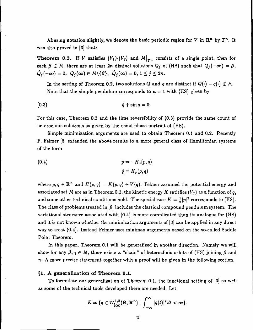
Abusing notation slightly, we denote the basic periodic region for V in R n by Tn. It

was also proved in [3] that:

Theorem 0.2. If V satisfies (Vi)-(V) and .MIT- consists of a single point, then for

each 3 E X4, there are at least 2n distinct solutions Qj of (HS) such that Qj(-oo) = 9,

j(-oo) = 0, Q,(oo) E M\{P}, ,(oo) = 0, 1 < j < 2n.

In the setting of Theorem 0.2, two solutions Q and q are distinct if Q(-) - q(.) 0 .M.

Note that the simple pendulum corresponds to n = I with (HS) given by

(0.3) 4 + sin q = 0.

For this case, Theorem 0.2 and the time reversibility of (0.3) provide the same count of

heteroclinic solutions as given by the usual phase portrait of (HS).

Simple minimization arguments are used to obtain Theorem 0.1 and 0.2. Recently

P. Felmer [8] extended the above results to a more general class of Hamiltonian systems

of the form

(0.4) = -1q(p,q)

4 = Hp(p,q)

where p,q E R' and H(p,q) = K(p,q) + V(q). Felmer assumed the potential energy and

associated set .M are as in Theorem 0.1, the kinetic energy K satisfies (V2 ) as a function of q,

and some other technical conditions hold. The special case K = -1p 2 corresponds to (HS).

The class of problems treated in [8] includes the classical compound pendulum system. The

variational structure associated with (0.4) is more complicated than its analogue for (HS)

and it is not known whether the minimization arguments of [3] can be applied in any direct

way to treat (0.4). Instead Felmer uses minimax arguments based on the so-called Saddle

Point Theorem.

In this paper, Theorem 0.1 will be generalized in another direction. Namely we will

show for any 0, -y E MN, there exists a "chain" of heteroclinic orbits of (HS) joining # and

-y. A more precise statement together with a proof will be given in the following section.

§1. A generalization of Theorem 0.1.

To formulate our generalization of Theorem 0.1, the functional setting of [3] as well

as some of the technical tools developed there are needed. Let

W 1 (R,R') J 1(t)I2dt < oo}.

2

Then E is a Hilbert space under the norm

(1.1) 0= (f 14 (t)1 2 dt + jq(O)12 )1/2

Note that q E E implies q is continuous on R.

To treat (HS), it can be assumed without loss of generality that

(1.2) OEMN{ and V(O)=O.

For q E E, set

(1.3) I(q) ('14(t)1 2 - V(q(t))) dt.-0

The heteroclinic solutions of (HS) were obtained in [3] as minima of I restricted to anappropriate subset of E. The following inequality (Lemma 3.6 of [3]) played a useful role

in that process. For A C R', let

Bp(A) = {x E R' I Ix - Al < p}.

Lemma 1.4: Let1

0<p<- min IC[.2 EM\{o}

Set

a(p)= min -V(x).vZB,(M)

If w E E and w(t) Z Bp(.M) for all t E [r,s], then

I(w) -> V2-ap)Cw(r) - w(s)l.

The next result is a small extension of Proposition 3.11 of [3]. It provides someregularity at ±00 for prospective initial points of I.

Proposition 1.5: If w E E and

L 21(blii - V(W)) to

(resp. J I__(! 2 - V(w)) dt < oo)

3

for some a E R, then w(oo) (resp. w(-oo)) E .

Now the class of sets on which I will be studied can be introduced. Let E satisfy:

(1.6) 0<,E< - mn3 fEM\{ol 3

and C E .M. Set

(1.7) 17,(e= {w E E jw(-oo) = 0,w(oo) = , and

w(t) B,(M\{0, e}) for all t E R}.

Define

(1.8) ce(C)= inf I(w)WEe r,)

and

(1.9) C~= inf c,().CE.\{0}

It was shown in [3] (Proposition 3.12) that

Proposition 1.10. For each e and as above, there is a q = q,, E F,(e) such that

I(q) = c,( ), i.e. q minimizes I~r( )"

Lemma 1.4 shows I(q ,) -+ oc as - o. Hence in (1.9) only finitely many numbers

C'( are involved and the infimum is in fact a minimum. If c, = c,( ) and q. = q,, so

I(q,) = c , simple comparison and regularity arguments given in [3] show

q.(t) fa B,(M\{o, }) = 0 for all t ER

provided that 1 is sufficiently small. Hence q, is the desired heteroclinic solution of (HS)

as claimed in Theorem 0.1.

Now our extension of Theorem 0.1 can be stated. For r7, E M, let

(1.11) r(, = {w E E I w(-oo) = vt,woc) =

and

(1.12) c(vl,. ) - inf l(w).wEr(,,)

4

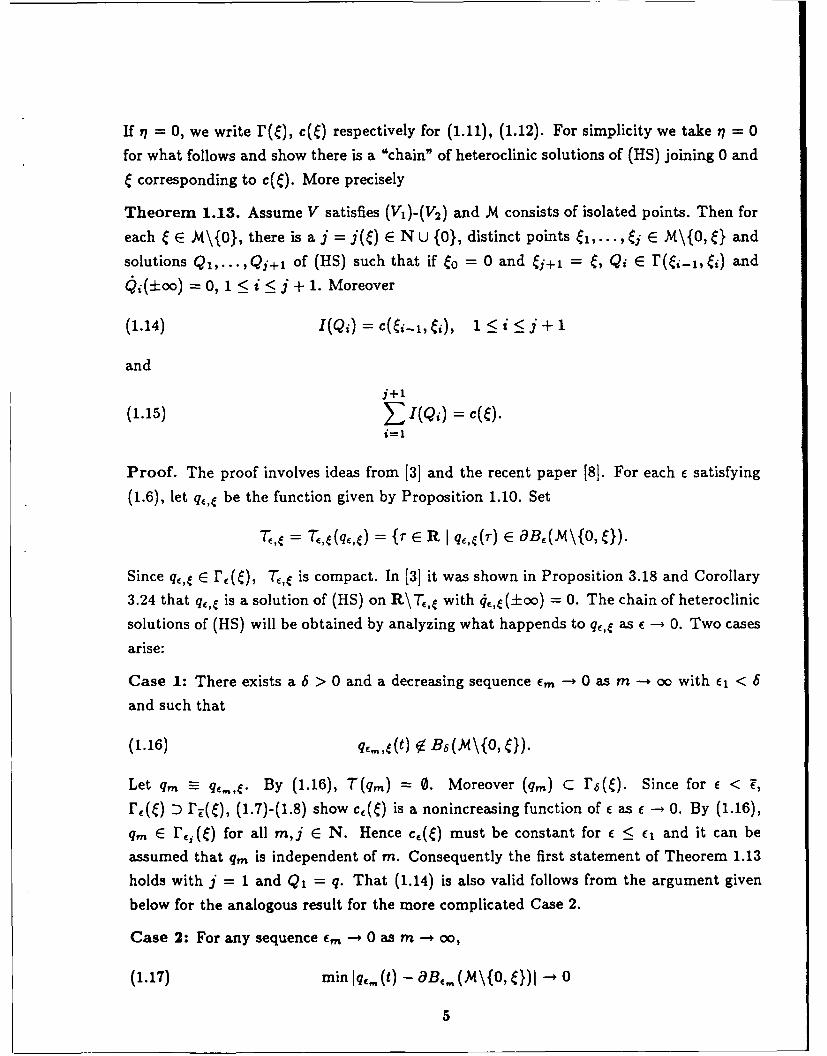
If v/ = 0, we write r(e), c( ) respectively for (1.11), (1.12). For simplicity we take r7 = 0

for what follows and show there is a "chain" of heteroclinic solutions of (HS) joining 0 and

e corresponding to c(e). More precisely

Theorem 1.13. Assume V satisfies (V 1)-(V 2 ) and .M consists of isolated points. Then for

each E .M\{0), there is a j = j( ) E N U {0}, distinct points 1,... , ej E .M\{0, } and

solutions Qi,... ,Q,+i of (HS) such that if O - 0 and j+i = e, Qi E r(i-, i) and

Qd(±oo) =0, 1 < i < j + 1. Moreover

(1.14) I(Qi) = CM-1~, i), < <i< j+l

and

j+1(1.5)ICQi )= mi=1

Proof. The proof involves ideas from [3] and the recent paper [8]. For each c satisfying

(1.6), let q ,, be the function given by Proposition 1.10. Set

= T,,(q) = {r E R I q,,(r) E aB,(M\{o,

Since q,, E IF,( ), T?,e is compact. In [3] it was shown in Proposition 3.18 and Corollary

3.24 that q ,, is a solution of (HS) on R\T, with 4,,(±oo) = 0. The chain of heteroclinic

solutions of (HS) will be obtained by analyzing what happends to qc,e as E --+ 0. Two cases

arise:

Case 1: There exists a 6 > 0 and a decreasing sequence E,, - 0 as m --- oo with E1 < 6

and such that

(1.16) qml,(t) 0 B 6 (M\{0, }).

Let qm - q,,,. By (1.16), T(qmn) == 0. Moreover (q,) C r6( ). Since for E < E,

I'e( ) D r,( ), (1.7)-(1.8) show c,( ) is a nonincreasing function of E as 6 --* 0. By (1.16),

q,, E r, ( ) for all m, j E N. Hence c,( ) must be constant for 6 < c and it can be

assumed that q, is independent of m. Consequently the first statement of Theorem 1.13

holds with j = 1 and Q, = q. That (1.14) is also valid follows from the argument given

below for the analogous result for the more complicated Case 2.

Case 2: For any sequence cm --+ 0 as m -* oo,

(1.17) min ,(t) - 49B,, (M\ {O, }-0

5

To prove Theorem 1.13 for this case, note first that qm is only determined up to a

phase shift. Indeed, for all t E R, qm(t + 0) E r. (C) and I(qm) = I(qm(t + 0)). Since

qrn E there is a unique sm E R such that qm(sm) E aBa(0) and qm(t) E B2.(O) for

t < s,,. Thus choosing 0 = si, it can be assumed that qm(O) E aB1 (0) and qm(t) E Ba(O)

for t < 0.

Next observe that by Lemma 1.4, whenever a segment of the curve q, joins aBE. (?7)

to aB,. ( ) for 77 5 " E .M, this segment makes a positive contribution to I(qm) whosemagnitude -- oo as IT/- J -+ co and which is bounded from below by a positive number

independently of m and of t7, E .M. By this observation and (1.17), it follows that there

is a j E N, precisely j points Ci,..., , E .M\{0, }, and a subsequence of m's such that

(1.18) mi Iqm(t) - ic 0

as rn - oo along this subsequence, 1 <: k < j. Moreover there is a 3 > 0 such that for

(1.19) main Iqm-t) -71 > / > 0tER

along the subsequence. By (1.18), there is a tm such that

(1.20) qm(tm,) - k, 1 < k <j

as m --+ oo along the subsequence. In fact tmk can be chosen so that it is the smallest

value of t satisfying

(1.21) Jqm(t) - ,kl = min Jqm(s) - kISER

along the subsequence. Passing to further subsequences if necessary, it can be assumed

that

(1.22) tmh > tm, for 1 < i < k

for all m along this subsequence.

Remark: See what follows repeated use of further subsequences will be necessary. Thiswill be evident from the context and so as not to belabor the exposition, we will make no

explicit mention of the fact other than this caveat.

Now the solutions QI... , Q,+I can be obtained. The construction will be dividedinto two steps. First we get Q1. Then, assuming Qi-1 i has been found, Qi will also be

constructed.

6

Set Qim(t) = qm(t), -0o < t < t,,. Then Qim is a solution of (HS) for this range

of t and even for a large interval if Iqm(t,,.) - elI > Em. Also

(i) Qim(o) EaBi (0)(1.23) (ii) Qm(t) E B 1(O),t < 0,

(iii) .l im(t)l2 + V(Qm(t)) = Ot < 0.

By Lemma 1.4, the functions q, are bounded in L=(R,Rn). Hence by (HS), (Ql m ) are

bounded in C 2((-o,tmi),Rn). Consequently by these bounds, (HS), and (1.23), Qim

converges in C 2 to a solution Q, of (HS) satisfyingloc

(i) Q 1(0) E aB x,(0).

(1.24) (ii) QI(t) E B3.(0),t < 0.2ii Q(t) 12 + V(Q1 (t)) = o, t < o.

Moreover by the C2 convergence, for any r < 0,

(1.25) fo (1.V 1(tI2_-V(Qi(t))) dt ,(

Hence

(1.26) ( I 2 - V(Q) dt < (

Therefore by Proposition 1.5, Qi(-oo) E M. Now (1.24) (ii) shows Ql(-0o) = 0 and

(1.24) (iii) implies (j (-oo) = 0.

It remains to find the range of values of t > 0 for which Q, is defined. Two cases will

be analyzed: (a) ti, -0 o asm -m o and (b) tin, has a bounded subsequence.

Case (a): tin, --+ o as m --+ 0o.

Then the above argument shows Qj m converges to Q, satisfying (HS) for all t E R,

(1.24) (iii) holds for all t E R, and

(1.27) [1I( i12 - V(Q,) dt < ,

Hence by Proposition 1.5, Ql(o) E .M. We claim Ql(oo) = 1. By (1.19), Qi( ) E

{j 1 0 < i < j+}. Suppose Ql(oo) = ei, i 5 1. Then Qj(s) - as s - o

for e.g. s E N. Since Qlm(s) -- QI(s) as m --- o, there is an m = r(s) such that

Qim(a)(.S) = qm(a)(s) --+ as s - 00. Now separate but related arguments are requiredto exclude the possibilities of i = 0 and i > 2.

7

If i = 0, for m = m(s), define

(128 ~WM(t)= 0 t < -1

(1.28) (t- (s-1))qm(s) s-1< t <sS qm(t) t>s.

Then wm E r . (e) and

(1.29) I(qm) -I(wm) f4M ( 1~2 - V(qm)) dt

- (11qm(sr 12 V(wm)) dt.

As s and therefore m -- oo, the second term in (1.29) approaches 0 since q, (s) - 0 while

by Lemma 1.4,

(1.30 f (!~rnI2- V(qm) dt > 2a (a )since for large m, the curve qm must join 0 to aB , (0) to aB6(0) to a neighborhood of 1.

Consequently for large s,

(1.31) I(qm) > I(wm),

contrary to Proposition 1.10. Hence i = 0 is not possible.

Next if QI(oo) = i, i > 2, let s and m(s) be as above. Let a E C'([0, 1],R'\B,(.M))

be a curve joining qm(s) to qm(tmi). Since qm(s) and qm(tmi) approaches i as s - oo,

we can assume cP,(t) ei i and b.(t) --+ 0 uniformly in t as s -+ oo. Define

W(t) =qm..(t) t< S(1.32) = P a t -s) a < t < S +- 1

= qm(t-a- 1 +tmi) t>S+1.

Then wm r,E. () and

'1.33) I(qm) - I(wm) = 1mI2 - v( m) dt

As s --. oo, the second term in (1.33) approaches 0 while

(1.34) j- (,dmI2-V(qm)) dt > 2 2o (2)

8

Thus for large s, (1.31) holds, again a contradiction.

Now for both cases we have shown QI(oo) = ei. Letting t -- oo in (1.24) (iii) yields

Q'(oc) = 0 and the first statement of Theorem 1.13 holds for Case (a).

Case (b). tml has a bounded subsequence. Then there is a r > 0 such that tm, - r.

Moreover Qlm(t) converges to Q 1 (t) in Cioc for t E (-oo,r) with Qi E C((-oo,rj,Rn),

Qi is a solution of (HS) for t < r, (1.24) (iii) holds for t < T, and Qi(r) = el. Letting

t r-* , (1.24) (iii) then shows that l(t) --* 0 as t --* r and (HS) implies 1(t) --+ 0 as

t -r T. These facts imply Qi can be extended in C 2 to [r, oo) as a solution of (HS) via

Q, (t) - ei for t > T.

Thus we have determined Qi for both Cases (a) and (b).

Remark 1.35: If V E C2 (Rn ,R), by the reasoning of Case (b) and the (then) uniqueness

of solutions of the initial value problem for (HS), Q 1 (t) = ei for t > r implies Q1 (t) - el

Hence Case (b) is not possible.

Remark 1.36: The argument given in Case (a) also shows Q 1 (t) $ ei, 0 < i < j 1

except possibly for i = 0 in a t interval containing -00 and i = 1 in a t interval containing

00.

It remains to show that (1.14) holds for Q,, i.e.

(1.37) I(Qi) =c( .

Since Q1 E r(ei),

(1.38) IWO, > c(el).

If equality does not hold in (1.38), there is a w E F(ej) such that

(1.39) I(w) < I(QI).

Define 6 by

(1.40) I(Q,) - I(w) = 56.

By a weak lower semicontinuity argument,

(1.41) Lo ( II2 - V(Q) dt < m (I14m'2 - V(qm) dt.

9

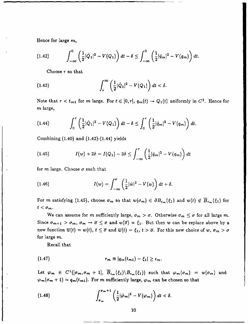
Hence for large m,

(1.42) J0 (1! l - v(Qi) dt -6 0 J4M ( 12 - V(qm)) dt.

Choose r so that

(1.43) i:' (1 J - V(Ql)) dt < 6.

Note that r < tin1 for m large. For t E [O,r], qm(t) -p Ql(t) uniformly in C2 . Hence for

m large,

(1.44) f~ lJ ( ~Vv(Q1)) dt - b J< ( 14 " 1 2 - V (qm)) dt.

Combining (1.40) and (1.42)-(1.44) yields

(1.45) I(w) + 2b = I(Ql) - 36 < J (l5 ,-, - V(qm)) dt

for m large. Choose a such that

(1.46) 1(w) = f (!i,1b2 - V(w) dt + 6.

For m satisfying (1.45), choose a so that w(am) E B,,,(I) and w(t) Z B for

t <am.

We can assume for m sufficiently large, am > a. Otherwise am < a for all large m.

Since am+, > urn, urn -U < a and w(U) = 1. But then w can be replace above by a

new function T(t) = w(t), t < U and T(t) = , t > U. For this new choice of w, a > a

for large m.

Recall that

(1.47) rm = Iq,-,(t,,,) - ell - E,,,.

Let cPm E Cl([am,am + 11, -Bi)\B,,([i)) such that pm(a,) = w(am) and

Vm(am + 1) = qm(tm). For m sufficiently large, pm can be chosen so that

148 + ml'- V(om))dt <b.

10

Set

(1.49) Wm (t) = w(t) t < am

= Vm(t) am <t <am+ l

=qm(t-am-1+tmi) t>am+l.

Then by construction Wm E rm( ). Moreover by (1.48)-(1.49),

(1.50) 1(w) _ I (ImI2 _ V(Wm) dt

Jm- (IkmI12 - V (Wm)) dt - 6.0

Hence by (1.45) and (1.50),

(1.51) JI 1Vml2 - v(wm) dt + 6 < (14m - V(qm) dt

for m large. Finally observe from (1.49) that

(1.52) (00 1 1I2 - V(Wm))dt= jt (141m2 - V(qm)) dt.

Adding (1.52) to (1.51) and recalling that tin1 > r for m large gives

(1.53) I(Wm) + 6 < I(qm).

But (1.53) violates the choice of qm in Proposition 1.10. Hence (1.37) holds

It remains to do the analogue of the above for Q2,. • •, Qj+. Suppose that Q,... Qi-ihave been constructed and (1.14) holds for these functions. We will show how to construct

Qt . Let im,i-1 be the largest value of t such that

(1.54) lqm(t) - il- = lq(tm,-l) - '1.

By the comparison argument of Case (a) following (1.26), it can be assumed that t,, >

tm,i-I for large m. Hence there is a ami E (tm,i-Itmi) such that

(1.55) qm(arn) EI qm (t) V RB,, ( -)t > ami.-

Define

(1.56) Qm (t) = qr,(t + om,t) t E (ii.._ - Ur 1, tmi- mi).

11

Then Qi.. satisfies (HS) for this range of t's and Qim(0) E OB, (Ci-i). As was the case

with Qim, these functions are bounded in C2 (tim,i-I -ami, tmi -ami, RI) and converge inC2 (for t in some maximal interval) to a solution Qi of (HS) such that Qi(O) E aB, (ei-1)

and Q (t) i Bj for t> 0.There are now 3 cases to consider

(i) Both sequences (tm,i-i - ami), (tmi - ami) are unbounded.

(ii) Only one sequence is unbounded.

(iii) Both sequences are bounded.

Case (1). Both sequences are unbounded.

Consequently, as with Q1, Qi satisfies (HS) on R and

(1.57) f ( ,J2_-V(Q,) dt l, )

for S = (-co,01 and [0, o). Proposition 1.5 then shows Qi(+oo) exists and belongs to .Moreover the arguments given for Qi show Qi(-oo) = i-. and Qi(oo) = i. Since Qi

satisfies (HS) on R,

(1.58) -1 1 (t)1 2 + V(Q,(t)) = constant = A, t E R.

Letting t -* -oo in (1.58) yields A > 0. By (1.57)-(1.58),

(1.59) CC, () f (A - 2V(Qi))dt > J Adt.

Hence A = 0. Therefore letting t - ±oo in (1.58) yields i(±oo) = 0.

To verify (1.14) for this case, we argue essentially as with Q1, the only difference being

that if i 5- j + 1, w(t) must be joined to q. both for large positive and negative values of

t. We omit the details.

Case (i1). Only one sequence is unbounded.

Suppose e.g. (t 1i - ain) is bounded. The arguments of Case (i) still show Qi(-oo) -

- and (1.58) holds for all t for which the solution is defined with A = 0. Since (tmi-rmii)

is bounded and Qim(tmi - ami) --* i as m -* oo, there is a r > 0 such that tmi - a 7i r

as m -+ oo and Qi(r) = i. Then by the arguments given for Case (b) of Q1, Qt extends

in a C 2 fashion as a solution of (HS) to [r, oo) via Qi(t) = Ci for t > r. We also get (1.14)

as in Case (i).

Case (iii). Both sequences are bounded.

12

As in Case (ii), there are constants a < 0 and r > 0 such that ti,t-1 - oram --+ o,

tmi - ami -+ r, Qi(a) = j-j, Q,(r) = ej, and Qj is a solution of (HS) on (a,r). We

can continuously extend Qj to R via Qi(t) = ei-1 for t < a and Qi(t) = &j for t > r.

We claim this extension belongs to C 2 (R,R ' ) (and therefore is a C2 solution of (HS)

with j(±oo) = 0). Equation (1.58) cannot be used as earlier to get a C 2 extension

since a prior A may be positive. Hence a more indirect approach will be employed. The

argument of Case (i) again implies (1.24) holds here. Now a slight variant of an argument

from Proposition 3.18 of [31 can be employed.

Let a < a and - > r. For V) E C 1 (R,R") with the support of ip in [z, ] and 6 E R,

the function Qj + 6¢b E r(i-l, ). By (1.14),

(1.60) I(Q + 6b) I(Qi).

Since (1.60) holds for all such 6 and tP,

(1.61) I'(Qi)kP (Q,. ik - V'(Qi) .ik)dt = 0

for all t E W012([aT],Rn). Thus Qi is a weak solution of the equation

(1.62) { ¢ + V ) =V'()o, , < t <f) Q() = i-i, Q(f) = 6.

But the inhomogeneous linear system (1.62) has a unique C 2 solution u which can be

written down explicitly. Taking the inner product with ? and integrating by parts implies

(1.63) (i. -V'(oQi).)at -0

for all iP E Wlo' 2 ([!,],Rn). Comparing (1.61) and (1.63) shows

(1.64) F( ,- i-). t =0

for all t E W0d'2 ([a,71,R"). Thus Qi is a weak solution of the equation

(1.62) +IQ = a tf

I Q(_) = i-i, Q(V) = C.

But the inhomogeneous linear system (1.62) has a unique C 2 solution u which can be

written down explicitly. Taking the inner product with i and integrating by parts implies

(1.63) (.1 - V'(Q,) . ik)dt = 0

13

for all k E Wo' 2 ([7,1],Rn). Comparing (1.61) and (1.63) shows

(1.64) f( o -16) . dt=O

for all 0 E WJ'02 ([21,?,Rn). But Qj - u belongs to this space. Consequently Q, = u on

[!ET], Q, E C 2 (R,Rn), and the construction of Qi is complete.

Finally to complete the proof of Theorem 1.13, (1.15) must be verified. By modifying

the functions Qi near el, Qj+i near ej, and Qj near ei-1 and ej, i - 1,j + 1, a function

Q E r(e) can be constructed such that I(Q) differs from F ' I/ (Qj) by an arbitrary small

amount. It follows that

j+l(1.65) CM <_ i(Qi).

If strict inequality held in (1.64), there is a w E r(e) such that

j+1(1.66) l(w) < i(Qi).

i=1

But then, by earlier arguments, for large m a function Tm E r,, () can be constructed

such that

j+1

(1.67) 1(UM) < I(Q= ).

Again, by earlier arguments, this leads to

(1.68) I(w) < I(qm) =c,.(e)

for large m, a constracziction.

The proof of Theorem 1.13 is complete.

References

[11 Mawhin, J. and M. Willem, Critical Point Theory and Hamiltonian systems, Springer

Verlag, 1989.

[21 Coti-Zelati, V., I. Ekeland, and E. Ser6, A variational approach to homoclinic orbits

in Hamiltonian systems, preprint.

14

[3] Rabinowitz, P.H., Periodic and heteroclinic orbits for a periodic Hamiltonian system,

Analyse nonlin{aire, 6 (1989), 331-346.

[4] Hofer, H. and K. Wysocki, First order elliptic systems and the existence of homoclinic

orbits in Hamiltonian-systems, preprint.

[5] Rabinowitz, P.H., Homoclinic orbits for a class of Hamiltonian systems, to appear

Proc. Royal Soc. Edinburgh.

[6] Benci, V. and F. Giannoni, Homoclinic orbits on compact manifolds, preprint.

[7] Tanaka, K., Homoclinic orbits for a second order Hamiltonian system, preprint.

[8] Felmer, P., Heteroclinic orbits for spatially periodic Hamiltonian-systems, preprint.

[9] Rabinowitz, P.H. and K. Tanaka, Some results on connecting orbits for a class of

Hamiltonian systems, preprint.

[10] Tanaka, K., Homoclinic orbits in a first order superquadratic Hamiltonian system:

convergence of subharmonic orbits, preprint.

15