henry’s law behavior and density functional theory analysis of adsorption...

HENRY’S LAW BEHAVIOR AND DENSITY FUNCTIONAL

THEORY ANALYSIS OF ADSORPTION EQUILIBRIUM

by

Bryan Joseph Schindler

Dissertation

Submitted to the Faculty of the

Graduate School of Vanderbilt University

in partial fulfillment of the requirements

for the degree of

DOCTOR OF PHILOSOPHY

in

Chemical Engineering

December, 2008

Nashville, Tennessee

Approved:

Professor M. Douglas LeVan

Professor Peter T. Cummings

Professor G. Kane Jennings

Professor Eugene J. LeBoeuf

Professor Kenneth A. Debelak

To my parents

ii

ACKNOWLEDGEMENTS

I would like to thank my advisor Dr. M. Douglas LeVan for all the time he

spent helping and guiding me and keeping me on track. This work would not have

happened without your help throughout.

I would like to thank Krista, Yu, Grant, and Joe and the rest of the people in

the lab for all their help inside and outside of the lab over the years. For answering

questions in the beginning, and distracting me when it was needed at the end. I also

want to thank Trey Wince, B.J. Feuerhelm, Matt Garvey, and Mark and Emily Eberle

for giving me a place to live during the last 6 months of my graduate experience.

I want to thank the US Army Edgewood Chemical and Biological Center for

funding my research. In particular I would like to thank Leonard Buettner, John

Mahle, David Tevault, Christopher Karwacki, and Tara Sewell for all of the help that

they provided.

My deepest thanks go to Dr. Peter Cummings for help with the math and

making sure that I maintained thermodynamic consistency. I also want to thank Dr.

Clare McCabe for her help with SAFT, and also Dr. Maria Carolina dos Ramos for

fitting the SAFT fluid parameters for nitrogen and n-pentane.

I would also like to thank the staff of the chemical engineering department.

For answerering questions and trying to look out for my best interests, I want to

thank Margarita Talavera and Mary Gilleran. Without the help from Mark Holmes,

finishing my research would have been much more difficult.

Without the support and backing of my family none of this would have been

possible. They were always there to listen and help in anyway that they could.

iii

TABLE OF CONTENTS

Page

DEDICATION . . . . . . . . . . . . . . . . . . . . . . . . . . . . . . . . . . . ii

ACKNOWLEDGEMENTS . . . . . . . . . . . . . . . . . . . . . . . . . . . . iii

LIST OF TABLES . . . . . . . . . . . . . . . . . . . . . . . . . . . . . . . . . vi

LIST OF FIGURES . . . . . . . . . . . . . . . . . . . . . . . . . . . . . . . . viii

I. INTRODUCTION . . . . . . . . . . . . . . . . . . . . . . . . . . . . . . 1

II. TRANSITION TO HENRY’S LAW IN ULTRA-LOW CONCENTRA-

TION ADSORPTION EQUILIBRIUM FOR N-PENTANE ON BPL AC-

TIVATED CARBON . . . . . . . . . . . . . . . . . . . . . . . . . . . . 9

2.1 Introduction . . . . . . . . . . . . . . . . . . . . . . . . . . . . . . . . 9

2.2 Experiments . . . . . . . . . . . . . . . . . . . . . . . . . . . . . . . . 12

Materials . . . . . . . . . . . . . . . . . . . . . . . . . . . . . . . . . . 12

Sample Preparation . . . . . . . . . . . . . . . . . . . . . . . . . . . . 13

Purge and Trap Apparatus . . . . . . . . . . . . . . . . . . . . . . . . 15

Operating Procedure . . . . . . . . . . . . . . . . . . . . . . . . . . . . 17

2.3 Results and Models . . . . . . . . . . . . . . . . . . . . . . . . . . . . 19

Adsorption equilibrium of n-pentane . . . . . . . . . . . . . . . . . . . 19

Dubinin–Radushkevich (DR) Equation . . . . . . . . . . . . . . . . . . 23

Langmuir Equation . . . . . . . . . . . . . . . . . . . . . . . . . . . . 25

Toth Equation . . . . . . . . . . . . . . . . . . . . . . . . . . . . . . . 26

2.4 Conclusions . . . . . . . . . . . . . . . . . . . . . . . . . . . . . . . . 30

III. THE THEORETICAL MAXIMUM ISOSTERIC HEAT OF ADSORP-

TION IN THE HENRY’S LAW REGION FOR SLIT-SHAPED CARBON

NANOPORES . . . . . . . . . . . . . . . . . . . . . . . . . . . . . . . . 37

3.1 Introduction . . . . . . . . . . . . . . . . . . . . . . . . . . . . . . . . 37

3.2 Theory . . . . . . . . . . . . . . . . . . . . . . . . . . . . . . . . . . 39

3.3 Results . . . . . . . . . . . . . . . . . . . . . . . . . . . . . . . . . . 40

3.4 Conclusions . . . . . . . . . . . . . . . . . . . . . . . . . . . . . . . . 48

IV. MODELING ADSORPTION OF NITROGEN AND PENTANE ON AC-

TIVATED CARBON USING SAFT-DFT . . . . . . . . . . . . . . . . . 53

4.1 Introduction . . . . . . . . . . . . . . . . . . . . . . . . . . . . . . . . 53

4.2 Theory . . . . . . . . . . . . . . . . . . . . . . . . . . . . . . . . . . . 54

iv

Model . . . . . . . . . . . . . . . . . . . . . . . . . . . . . . . . . . . 54

Model Validation . . . . . . . . . . . . . . . . . . . . . . . . . . . . . 59

Parameter Estimation for Real Fluids . . . . . . . . . . . . . . . . . . 61

4.3 Results . . . . . . . . . . . . . . . . . . . . . . . . . . . . . . . . . . . 65

Nitrogen . . . . . . . . . . . . . . . . . . . . . . . . . . . . . . . . . . 65

Pentane . . . . . . . . . . . . . . . . . . . . . . . . . . . . . . . . . . 74

4.4 Conclusions . . . . . . . . . . . . . . . . . . . . . . . . . . . . . . . . 83

V. CONCLUSIONS AND RECOMMENDATIONS . . . . . . . . . . . . . 90

Appendix

A. SAMPLE PREPARATION . . . . . . . . . . . . . . . . . . . . . . . . . 94

A.1 Initial preparation work . . . . . . . . . . . . . . . . . . . . . . . . . . 94

A.2 Liquid Injection . . . . . . . . . . . . . . . . . . . . . . . . . . . . . . 94

A.3 Gas Injection . . . . . . . . . . . . . . . . . . . . . . . . . . . . . . . 95

B. OPERATION PROCEDURE FOR THE DYNATHERM SYSTEM . . . 96

C. EXPERIMENTAL SETTINGS . . . . . . . . . . . . . . . . . . . . . . . 99

D. DENSITY FUNCTIONAL EQUATIONS . . . . . . . . . . . . . . . . . 101

D.1 DFT . . . . . . . . . . . . . . . . . . . . . . . . . . . . . . . . . . . . 101

D.2 Bulk Fluid . . . . . . . . . . . . . . . . . . . . . . . . . . . . . . . . . 106

D.3 Model Validation . . . . . . . . . . . . . . . . . . . . . . . . . . . . . 108

E. ANALYSIS OF ALTERNATIVE NITROGEN ADSORPTION DATA BY

SAFT-DFT . . . . . . . . . . . . . . . . . . . . . . . . . . . . . . . . . 111

v

LIST OF TABLES

2.1 Previously measured low concentration data by descending pure compo-

nent vapor pressure of chemical . . . . . . . . . . . . . . . . . . . . . . . 10

2.2 Experimental data for adsorption of n-pentane on BPL activated carbon 20

2.3 Model parameters for the Langmuir and Toth equations . . . . . . . . . 29

2.4 Calculated isosteric heats of adsorption . . . . . . . . . . . . . . . . . . . 29

3.1 Model Parameters for Different Molecules . . . . . . . . . . . . . . . . . 42

3.2 Isosteric Heat of Adsorption in the Henry’s Law Region . . . . . . . . . 46

4.1 Model parameters . . . . . . . . . . . . . . . . . . . . . . . . . . . . . . 65

C.1 HP 5890 Series II GC Settings . . . . . . . . . . . . . . . . . . . . . . . 99

C.2 Dynatherm settings . . . . . . . . . . . . . . . . . . . . . . . . . . . . . 100

vi

LIST OF FIGURES

1.1 Hexane isotherms extended to lower pressures . . . . . . . . . . . . . . . 4

2.1 Schematic of the sample preparation apparatus: (a) liquid injection and

(b) gas injection. . . . . . . . . . . . . . . . . . . . . . . . . . . . . . . . 14

2.2 Schematic of the apparatus to analyze the samples. . . . . . . . . . . . . 16

2.3 n-Pentane on BPL activated carbon with the Toth equation: (a) isotherm

and (b) Henry’s law plot. . . . . . . . . . . . . . . . . . . . . . . . . . . 22

2.4 n-Pentane on BPL activated carbon with the DR, Langmuir, and Toth

equations: (a) isotherm and (b) Henry’s law plot. . . . . . . . . . . . . . 24

2.5 Adsorption isosteres for n-pentane on BPL activated carbon with liquid

vapor pressure. . . . . . . . . . . . . . . . . . . . . . . . . . . . . . . . . 28

2.6 Isosteric heat of adsorption vs. loading. These can be compared with the

heat of vaporization of 25.79 kJ mol−1 for n-pentane at the normal boiling

point. . . . . . . . . . . . . . . . . . . . . . . . . . . . . . . . . . . . . . 31

3.1 Model of graphite parallel slit pore. Carbon atoms continue deep into solid. 41

3.2 The isosteric heat of adsorption in the Henry’s law region as a function of

pore width. . . . . . . . . . . . . . . . . . . . . . . . . . . . . . . . . . . 44

3.3 The effects of σsf and εsf on the pore width of the maximum heat of

adsorption. . . . . . . . . . . . . . . . . . . . . . . . . . . . . . . . . . . 45

4.1 Hard sphere 3-mers against a hard wall . . . . . . . . . . . . . . . . . . . 60

4.2 Hard sphere 4-mers against a hard wall . . . . . . . . . . . . . . . . . . . 62

4.3 Hard sphere 20-mers against a hard wall . . . . . . . . . . . . . . . . . . 63

4.4 Attractive sphere 3-mers against a hard and attractive wall . . . . . . . 64

vii

4.5 Comparison of experimental and theoretical adsorbed volumes of nitrogen

on nonporous carbon black at 77 K. The points are experimental data.

The solid line is the model prediction. . . . . . . . . . . . . . . . . . . . 66

4.6 Nitrogen density profiles in a 0.564 nm pore. . . . . . . . . . . . . . . . . 68



4.9 Full pore width density profile of nitrogen at 77 K. . . . . . . . . . . . . 72

4.10 Average density profile of nitrogen 77 K. . . . . . . . . . . . . . . . . . . 73

4.11 Pore size distribution calculated from nitrogen density profiles. . . . . . 75

4.12 Nitrogen isotherm at 77 K on BPL activated carbon. Solid line is the

calculated isotherm. . . . . . . . . . . . . . . . . . . . . . . . . . . . . . 76

4.13 Comparison of experimental and theoretical adsorbed volumes of pentane

on nonporous carbon black at 293.15 K. The points are experimental data.

The solid line is the model predictions. . . . . . . . . . . . . . . . . . . . 77

4.14 n-pentane density profiles in a 4.81 A pore. . . . . . . . . . . . . . . . . 78

4.15 n-pentane density profiles in a 6.07 A pore. . . . . . . . . . . . . . . . . 79

4.16 The average density profile for n-pentane at 298.15 K. . . . . . . . . . . 81

4.17 Calculated n-pentane isotherm at 25oC on BPL activated carbon. . . . . 82

D.1 Hard spheres on hard wall. . . . . . . . . . . . . . . . . . . . . . . . . . 109

E.1 Pore size distribution calculated from nitrogen density profiles. . . . . . 112

E.2 Nitrogen isotherm at 77 K on BPL activated carbon. Solid line is the

calculated isotherm. . . . . . . . . . . . . . . . . . . . . . . . . . . . . . 113

E.3 Calculated n-pentane isotherm at 25oC on BPL activated carbon. . . . . 114

viii

CHAPTER I

INTRODUCTION

Over the last few decades there has been an increased use of adsorption industrially

in the separation of gases and liquids. One reason for this is the development and

improvement of adsorption processes and materials. Adsorption can offer a more

economically viable separation method for gases over other methods, such as cryogenic

distillation. One of the reasons adsorption is gaining popularity as an alternative for

separation is because of the diversity in adsorbent materials and how they operate

at a variety of conditions. However, the large number of variables involved can make

optimizing designs complex and require knowledge in a number of different aspects

of adsorption.

Adsorption is used in many different types of processes. Some examples are

bulk separation, gas storage, purification, and trace contaminant removal. Oxygen

enrichment from air is an example of a bulk separation process. In the last few

years there has been a increase in the amount of research done using adsorption for

gas storage as a fuel supply for vehicular use. Specifically, the interest is in the

ability to store large amounts of natural gas or hydrogen at moderate pressures and

temperatures. Some examples of purification are the removal of by-products other

than hydrogen from the process stream of the gas water shift reaction where carbon

monoxide and water are reacted to form carbon dioxide and hydrogen, or the removal

of nitrogen and carbon dioxide from a methane stream. Trace contaminant removal

of impurities from a process stream is another common adsorption process that has

seen an increase in interest, especially as part of a HVAC system.

All adsorption processes require knowledge of the two main separation mech-

anisms, equilibrium and kinetics, in order to achieve an effective design. When the

1

process is driven by the kinetics of the system the mechanisms can be steric, in-

volving the exclusion of molecules based on size and shape, or by the differences in

rate of adsorption and desorption. However, for most processes equilibrium factors

are of primary concern. Equilibrium data in the form of adsorption isotherms gives

the relative amounts that the adsorbent material can adsorb at a given pressure for

single and multicomponent systems. Also the slopes of the isotherms in the regions

of interest are important for design as they determine the regenerability of the solid

adsorbent materials. Sets of isotherms at different temperatures allow the calculation

of the isosteric heat of adsorption, which is important to the behavior of the system

as it cycles between adsorption and desorption. Identifying the materials with the

correct capacity, selectivity, and kinetics is extremely important to the design of an

adsorption-based separation process.

Measurements of adsorption equilibrium and kinetics are achieved by a number

of methods. The most commonly used methods for measuring adsorption equilibrium

are volumetric and gravimetric. Volumetric methods fall into two different categories.

In the first category, a known amount of adsorbate and adsorbent are introduced into a

system of known volume and the resulting pressure is measured. This method works

well for single component systems, but does not work as well for multicomponent

systems. The second method of performing a volumetric experiment is by adding

a gas chromatograph (GC) to the system allowing for an analysis of the gas phase.

This setup works well for multi-component systems.

Gravimetric methods for measuring adsorption isotherms operate in a differ-

ent manner. The loading of a sample in the system is measured by an accurate

microbalance as adsorbate is introduced. Pressure is measured with a transducer.

However, both systems do not have the required accuracy to measure data

into the Henry’s law region except for light gases. The volumetric system is limited

by the accuracy of the pressure transducer or by the lower limit of the detector on

2

the GC and the maximum volume injectable into the GC. Gravimetric systems are

best reserved for single component systems. They are limited by the accuracy of the

microbalance, typically 1.0 µg or 0.1 µg.

The kinetics of a system can be measured by a number methods. A commonly

used method is the use of uptake curves from a gravimetric system; however, this

method is not very accurate and cannot discriminate between mechanisms. Some of

the newer methods are differential bed adsorption, zero-length column, and frequency

response.

The ability to model complex systems accurately is a driving force behind

adsorption research. It is desirous to have a model that can predict the behavior

of single and multicomponent systems without having to do experiments, especially

for systems that can be very dangerous or corrosive. In particular, it would be

beneficial to have the model based on known parameters such as a Lennard-Jones

diameter σ and well depth ε. A long term goal of adsorption theory is to be able

to accurately predict adsorption equilibrium from first principles based on knowledge

of the structure of the adsorbing molecule and the structure and composition of the

adsorbent.

With the continual lowering of exposure levels to volatile organic compounds

(VOCs) and toxic industrial compounds (TICs), the use of adsorption-based removal

systems is receiving more attention as a viable option. However, there is scant data

on most VOCs at and below the level that will be required to design these systems

effectively. In many cases, adsorption isotherms will be required into the Henry’s

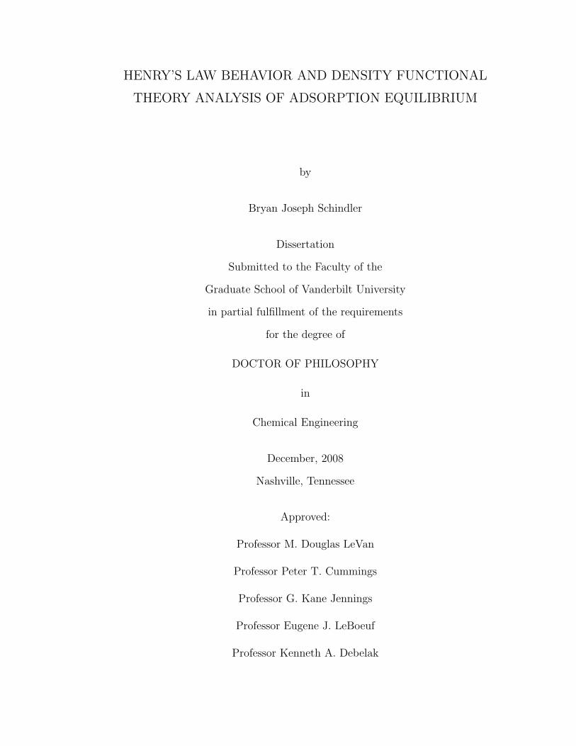
law region. An example of why data are needed is provided in Fig. 1.1, which shows

two sets of hexane data1,2 between saturation and 0.3 mol kg−1. Also included are

four different adsorption isotherms: group contribution theory,3 virtual group the-

ory,4 Dubinin-Radushkevich (DR),5 and the Toth equation.6 There is considerable

agreement between the data and the models over the range where there is data. How-

3

0.001

0.01

0.1

1

10

Load

ing

(mol

/kg)

10-12 10-10 10-8 10-6 10-4 10-2 100 102

Pressure (kPa)

Hacskaylo Pigorini GCT VGT DR Toth

Line of slope 1

25 C

Figure 1.1: Isotherm of n-hexane on BPL activated carbon with the group contribu-tion theory, virtual group theory, DR equation, and the Toth equation.

4

ever, when the isotherm is extended to lower loadings there is considerable spread

between the predicted pressure of the models. If these models were used to design an

adsorption filtration device for the removal to ultra-low concentrations there would

be considerable differences between the four models. This demonstrates the need for

adsorption data at much lower concentrations to determine which model, if any, is

correct.

In Chapter II we discuss the development of a novel method for preparing

samples at known loadings and analyzing these samples, which reach into the Henry’s

law region. Samples were prepared at loadings from 1.0 down to 0.0001 mol kg−1 for

n-pentane on BPL activated carbon. The samples from 1.0 to 0.01 mol kg−1 were

prepared using a liquid injection system. The samples below 0.01 mol kg−1 were

prepared with a gas injection system. After a sample was prepared with either method

it was sealed and allowed to come to equilibrium at an elevated temperature. The

samples were then analyzed using a purge and trap method. Adsorption isotherms

were measured over a wide range of temperatures, from 0 to 175 oC at constant

loading, using a novel apparatus that concentrates the gas phase of n-pentane from

a large volume to a much smaller volume. The measured data are used to analyze

the behavior of three different adsorption isotherms, the DR equation, the Langmuir

equation, and the Toth equation. We will discuss how these theories describe the

data as they transition into the Henry’s law region. The isosteric heat of adsorption is

calculated and discussed as a function of the loading. This is the first time adsorption

equilibrium has been measured in the Henry’s law region for an adsorbate that is a

liquid at room temperature.

In Chapter III the isosteric heat of adsorption in the Henry’s law region is cal-

culated as a function of pore width for a variety of gases. These values are compared

with the isosteric heat of adsorption calculated from adsorption isotherms. These

data, and specifically the maximum value, are important in the design of new mate-

5

rials. The isosteric heat of adsorption, in the Henry’s law region in particular, gives

important information about mechanisms and properties of adsorption. When de-

signing a new material, especially if it is for a specific process, knowing which pore

sizes to emphasize or avoid can be very helpful. In the design of a trace contaminant

removal system you would want a system with pores as close as possible to the pore

size that gives the maximum isosteric heat of adsorption. This would provide the

system with the maximum amount of retention of the contaminants. However, if you

are designing a pressure swing adsorption system a low isosteric heat of adsorption

would be preferable to reduce heat effects and allow more efficient regeneration. In

gas storage, heat of adsorption can be used as a screen to eliminate materials that

would not reach the desired deliverable capacity because of overheating during ves-

sel charging and overcooling during vessel discharge. The use of knowledge of the

isosteric heat of adsorption in the Henry’s law region in the initial design of new

materials will allow for more targeted development to specific problems, which will

result in more effective materials.

The ability to predict adsorption isotherms using fundamental information

about the adsorbate and adsorbent is an important research goal. In Chapter IV,

density functional theory (DFT) is modified to allow the modeling of chain molecules

using the statistical associating fluid theory (SAFT) equation of state. This will be

the first time that a mean-field for the first order attractive term is not assumed, and

it is also the first time that the second order term is included. DFT has been widely

used to model the adsorption of spherical molecules in parallel or cylindrical pores.

By changing the equation of state from a spherical to SAFT we are able to model the

behavior for a much larger array of molecules. This allows us to predict adsorption

behavior given the bulk parameters, the interaction of the adsorbate molecule with

graphite, and the pore size distribution of the adsorbent.

Parameters were estimated to describe the bulk behavior and the interaction

6

with a carbon wall for nitrogen and n-pentane. Density profiles for nitrogen show

the adsorption behavior of nitrogen in a variety of pore sizes at different pressures.

The monolayer transition, capillary condensation, and the freezing transition are

discussed. This is the first time, that we are aware of, that such a sharp freezing

transition is demonstrated. The density profiles are used to calculate a pore size

distribution for BPL activated carbon. Density profiles were then calculated for n-

pentane. Using the density profiles and the calculated pore size distribution, an

isotherm for n-pentane was determined.

In Chapter V, the conclusions from this work are summarized. Also included

are recommendations for follow up work that result from this dissertation.

7

References

[1] Hacskaylo JJ. Thermodynamic Studies of Vapor-Solid Adsorption Equilibria.

Charlottesville VA USA, University of Virginia , Ph.D. thesis, 1987.

[2] Pigorini G. Periodic Behavior of Pressure Swing Adsorption Cycles and Coad-

sorption of Light and Heavy n–alkanes on Activated Carbon. Charlottesville VA

USA, University of Virginia , Ph.D. thesis, 2000.

[3] Walton KS, Pigorini G, and LeVan MD. Simple group contribution theory for

adsorption of alkanes in nanoporous carbons. Chem. Eng. Sci. 2004: 59:(4425–

4432)

[4] Ding Y. Periodic adsorber optimization and adsorption equilibrium measurement

and prediction. Nashville TN USA, Vanderbilt University , Ph.D. thesis, 2002.

[5] Ye XH, Qi N, Ding YQ, LeVan MD. Prediction of Adsorption Equilibrium using

a Modified D-R Equation: Pure Organic Compounds on BPL Carbon. Carbon

2003; 41:681–686

[6] Do DD. Adsorption Analysis: Equilbria and Kinetics. London: Imperial College

Press; 1998

8

CHAPTER II

TRANSITION TO HENRY’S LAW IN ULTRA-LOW CONCENTRATION

ADSORPTION EQUILIBRIUM FOR N-PENTANE ON BPL ACTIVATED

CARBON

2.1 Introduction

The use of adsorption for the removal of volatile organic compounds (VOCs)

and toxic industrial chemicals (TICs) has drawn considerable attention in recent years.

With rising health concerns leading to the continual lowering of allowable exposure

levels for VOCs and TICs, the use of microporous adsorbent materials to remove

these chemicals will increase. To design air filters to remove ultra-low concentrations

of contaminants, adsorption equilibrium data will be required at lower concentrations

than are currently available, including into the Henry’s law region. Also, contaminants

bleed through filters receiving occasional exposures to VOCs and TICs, and low

concentration adsorption equilibrium is necessary to analyze this process accurately.

However, standard volumetric and gravimetric methods do not have the sensitivity

necessary to obtain these measurements, especially for low-vapor pressure compounds,

e.g., chemicals that are liquids at room temperature and pressure.

Most adsorption data at low concentrations are measured by either gravimetric

or volumetric methods. Foster et al.,1 Pinto et al.,2 and Kuro-Oka3 used a gravimetric

method to measure adsorption of light and heavy gases on activated carbons. See

Table 2.1 for details. The resolution of gravimetric methods is limited by the accuracy

of the microbalance, which is typically 1.0 µg or 0.1 µg.

The volumetric method has also been used extensively. Eissmann and LeVan,4

Kaul,5 Mahle et al.,6 Russell and LeVan,7 Karwacki and Morrison,8 Pigorini,9–11 Zhu

et al.12,13 and many others have measured adsorption equilibria for high-vapor pres-

sure gases on activated carbons. Golden and Kumar14 measured trace concentrations

9

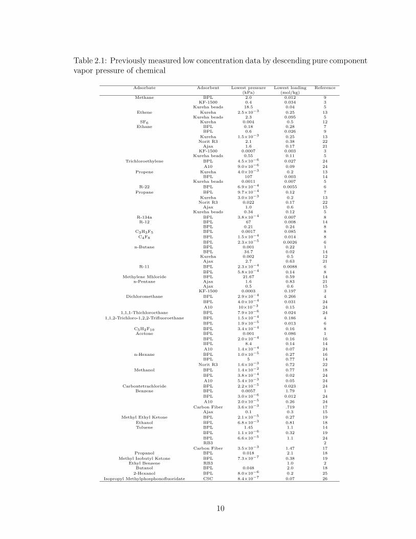
Table 2.1: Previously measured low concentration data by descending pure componentvapor pressure of chemical

Adsorbate Adsorbent Lowest pressure Lowest loading Reference(kPa) (mol/kg)

Methane BPL 2.0 0.012 9KF-1500 0.4 0.034 3

Kureha beads 18.5 0.04 5

Ethene Kureha 2.5×10−3 0.25 13Kureha beads 2.3 0.095 5

SF6 Kureha 0.004 0.5 12Ethane BPL 0.18 0.28 7

BPL 0.6 0.026 9

Kureha 1.5×10−3 0.25 13Norit R3 2.1 0.38 22

Ajax 1.6 0.17 21KF-1500 0.0007 0.003 3


Trichloroethylene BPL 4.5×10−6 0.027 24

A10 9.0×10−6 0.09 24

Propene Kureha 4.0×10−3 0.2 13BPL 107 0.003 14


R-22 BPL 6.9×10−4 0.0055 6

Propane BPL 9.7×10−4 0.12 7

Kureha 3.0×10−3 0.2 13Norit R3 0.022 0.17 22

Ajax 1.0 0.6 15Kureha beads 0.34 0.12 5

R-134a BPL 3.8×10−4 0.007 8R-12 BPL 67 0.008 14

BPL 0.21 0.24 8C3H3F5 BPL 0.0017 0.085 8

C4F8 BPL 1.5×10−4 0.014 8

BPL 2.3×10−5 0.0026 6n-Butane BPL 0.001 0.22 1

BPL 34.7 0.02 14Kureha 0.002 0.5 12Ajax 2.7 0.63 21

R-11 BPL 2.3×10−4 0.0088 6

BPL 5.8×10−4 0.14 8Methylene Mhloride BPL 21.67 0.59 14

n-Pentane Ajax 1.6 0.83 21Ajax 0.5 0.6 15

KF-1500 0.0003 0.197 3

Dichloromethane BPL 2.9×10−4 0.266 4

BPL 4.0×10−4 0.031 24

A10 10×10−3 0.15 24

1,1,1-Thichloroethane BPL 7.9×10−6 0.024 24

1,1,2-Trichloro-1,2,2-Trifluoroethane BPL 1.5×10−4 0.186 4

BPL 1.9×10−5 0.013 6

C5H2F10 BPL 3.4×10−4 0.16 8Acetone BPL 0.001 0.086 1

BPL 2.0×10−4 0.16 16BPL 8.4 0.14 14

A10 1.4×10−4 0.07 24

n-Hexane BPL 1.0×10−5 0.27 16BPL 5 0.77 14

Norit R3 1.6×10−3 0.72 22

Methanol BPL 1.4×10−2 0.77 18

BPL 3.8×10−4 0.02 24

A10 5.4×10−3 0.05 24

Carbontetrachloride BPL 2.2×10−5 0.023 24Benzene BPL 0.0057 1.79 1

BPL 3.0×10−6 0.012 24

A10 2.0×10−5 0.26 24

Carbon Fiber 3.6×10−3 .719 17Ajax 0.1 0.3 15

Methyl Ethyl Ketone BPL 2.1×10−5 0.27 19

Ethanol BPL 6.8×10−3 0.81 18Toluene BPL 1.45 1.1 14

BPL 1.1×10−6 0.32 19

BPL 6.6×10−5 1.1 24RB3 2

Carbon Fiber 3.5×10−3 1.47 17Propanol BPL 0.018 2.1 18

Methyl Isobutyl Ketone BPL 7.3×10−7 0.38 19Ethyl Benzene RB3 1.0 2

Butanol BPL 0.048 2.0 18

2-Hexanol BPL 8.0×10−6 0.2 25

Isopropyl Methylphosphonofluoridate CSC 8.4×10−7 0.07 26

10

of high and low vapor pressure gases in a carbon dioxide stream. Do and Do15 mea-

sured adsorption isotherms for both low and high vapor pressure gases. Rudisill et

al.,16 Yun et al.,17 Taqvi et al.,18 Qi and LeVan,19 and others have measured ad-

sorption equilibria for low-vapor pressure gases on activated carbons, with the lowest

pressures and loadings given in Table 2.1.

Other methods for measuring adsorption isotherms have also been used. Yang

et al.20 used temperature programmed desorption to estimate an adsorption isotherm

for dioxins on activated carbon. Mayfield and Do21 used a differential adsorption

bed to measure isotherms for ethane, butane, and pentane on Ajax activated car-

bon. Linders et al.22 used head space gas chromatography to measure nitrogen,

ethane, propane, and hexane isotherms on Norit R3. Himeno and Urano23 and Hi-

meno and Kohei24 used headspace gas chromatography for benzene, dichloromethane,

trichloroethylene, carbon tetrachloride, 1,1,1-trichloroethane, and methanol on BPL,

CQS, and A10 carbons. Karwacki et al. 25 used a purge and trap method to measure

2-hexanol equilibrium on BPL carbon. Karwacki et al. 26 also measured isotherms

for isopropyl methylphosphonofluoidate (GB) on a coconut-based activated carbon

using the same method.

Prior measurements of low limits for adsorption equilibrium of VOCs can be

indicated in terms of pressure or loading. From Table 2.1, the lowest pressure mea-

sured previously for a high-vapor pressure VOC, obtained by Himeno and Kohei24

for trichloroethylene on BPL carbon, is 4.5× 10−6 kPa and for a low-vapor pressure

VOC, measured by Qi and LeVan19 for methyl isobutyl ketone on BPL carbon, is

7× 10−7 kPa. The lowest loading previously measured for a high-vapor pressure gas,

obtained by Mahle et al. 6 for R-318 on BPL carbon, is 0.0026 mol kg−1 and for a

low-vapor pressure gas, reported by Himeno and Kohei24 for benzene on BPL carbon,

is 0.012 mol kg−1.

Measuring adsorption data in the Henry’s law region has been difficult. There

11

have been reported instances where Henry’s law was achieved for light gases. For

example, Pigorini9 measured data into the Henry’s law region for methane and ethane

on BPL activated carbon. Eissmann and LeVan4 reached the Henry’s law region for

R-113 and approached Henry’s law for dichloromethane on BPL activated carbon.

Kaul5 measured methane, ethane, ethene, and propene on Kureha beads into the

Henry’s law region. Mahle6 achieved Henry’s law for R-22 and approached Henry’s

law for R-318 on BPL activated carbon. There are no reported cases of adsorption

of low-vapor pressure gases in the Henry’s law region.

In this paper, we use a purge and trap method to extend the lower limits of

adsorption equilibria into the Henry’s law region for a low-vapor pressure gas. We

propose new methods to prepare pre-equilibrated samples at known loadings from 1.0

to 0.0001 mol kg−1. To analyze the samples we use the method described by Karwacki

et al.26 The adsorption isotherms will be compared with the Dubinin-Radushkevich

(DR) equation, the Langmuir equation, and the Toth equation. The transition into

the Henry’s law region will be discussed for each of the theories. The isosteric heat

of adsorption will also be evaluated and discussed. To our knowledge this is the first

report of adsorption equilibrium being measured into the Henry’s law region for a

low-vapor pressure gas.

2.2 Experiments

Materials

The activated carbon used in these experiments was type BPL (Calgon Carbon

Corp., Lot No. 4814-J) in 40 × 50 mesh. The adsorbate was n-pentane (HPLC Grade,

99% min). The adsorbents used in the thermal desorption unit were CarbotrapTM

Graphitized Carbon Black in 20 × 40 mesh in the sample tube and CarbopackTM X

in 20 × 40 mesh in the focusing trap.

12

Sample Preparation

For these experiments, pre-equilibrated samples were prepared at known load-

ings. The methods used to prepare these samples involved a liquid injection or a gas

injection into an evacuated glass ampule containing regenerated carbon. The liquid

injection system was used for samples with loadings greater than or equal to 0.01 mol

kg−1, while the gas injection system was used for samples with loading less than or

equal to 0.01 mol kg−1. Samples were prepared by both methods at a loading of 0.01

mol kg−1 to verify that the injection methods were equivalent.

BPL activated carbon was regenerated at 200 oC with a helium purge at a flow

rate of 0.5 L min−1 for at least 8 h. Then, approximately 2 g of carbon was placed

in a pre-numbered, pre-weighed glass ampule and weighed. The ampules were then

connected to a dosing apparatus for liquid or gas injection.

A diagram of the dosing apparatus used to prepare a sample by liquid injection

is shown in Figure 2.1a. The ampule was connected, heated to 150 oC, and placed

under vacuum for eight hours to regenerate the sample a second time. A rotary-vane

vacuum pump was used to achieve a vacuum of approximately 0.05 mbar. The ampule

was removed from the heat, placed in an ice bath, and the valve shown in Figure 2.1a

was closed, removing the sample from the vacuum. A syringe was used to inject a

known amount of adsorbate into the ampule. The syringe was weighed before and

after injection to determine the mass injected. The glass ampule was then sealed with

a micro-torch and weighed with waste glass for calculation of the mass of adsorbent.

A diagram of the gas dosing system used to prepare samples at the lowest

loadings is shown if Figure 2.1b. Instead of injecting liquid with a syringe, a saturated

vapor was generated and injected using a gas sampling loop. To accomplish this, the

ampule was connected to the apparatus, heated to 150 oC, and placed under vacuum

for eight hours to regenerate it a second time as described above. The temperature

of the temperature bath shown in Figure 2.1b and the size of the sample loop were

13

Vacuum

Septum

a

To Vacuum

Temperature Bath

Needle Valve

Pressure Transducer

Adsorbate

Sample Loop

Adsorbent

6 port Valve

Vacuum

b

Figure 2.1: Schematic of the sample preparation apparatus: (a) liquid injection and(b) gas injection.

14

determined by the desired loading with minimums of –4.0 oC and 25 µl used for the

lowest loading. A vacuum was connected to the adsorbate vapor generator to remove

any impurities (e.g., dissolved gases) from the system, and the pressure transducer

was used as a check on the vapor pressure. When the adsorbate was at the expected

vapor pressure, the adsorbent sample was removed from the vacuum and was placed

in an ice bath. The six-port valve was switched, thereby isolating the loop from the

vapor generating side and exposing the adsorbent to the n-pentane vapor. The ampule

was then sealed with the micro-torch and weighed with waste glass to determine the

mass of adsorbent used.

After a sample had been prepared by the methods described above, the sealed

glass ampule was leak tested by submerging it in water. Ampules were then strapped

to a ferris wheel arrangement in an environmental chamber, heated to 150 oC, and

rotated end-over-end at 4 rpm for days to months to increase the mixing of the solid

and gas phases as equilibrium was established.

Purge and Trap Apparatus

A diagram of the apparatus used to analyze the equilibrated samples is shown

in Figure 2.2. The adsorption bed was placed inside an environmental chamber (Ther-

motron SE-300-2-2) to control the temperature of the sample. A mass flow controller

was used to set the flow rate of nitrogen carrier gas through the sample. As the carrier

gas flowed through the sample in the adsorption bed, the adsorbate in the gas phase

was removed from the small fixed bed. A nitrogen bypass line was created by use of

the open tee, which maintained the pressure in the system. The bypass line was set

at a flow rate such that there was always a positive flow out of the open tee, keeping

the system clean of any impurities.

The carrier gas containing n-pentane vapor flowed into the thermal desorption

unit (Dynatherm model ACEM 900), which has two adsorption beds in series, the

15

MFC MFC

Thermal Desorption

System

Environmental Chamber

Adsorption Bed

Open Tee

Carrier Gas

Carrier Gas Vacuum

GC

Nitrogen By-Pass

Figure 2.2: Schematic of the apparatus to analyze the samples.

16

sample tube and the focusing trap. The materials for these adsorption beds were

chosen to remove the n-pentane from the gas phase at room temperature and release

the n-pentane at high temperature. The n-pentane is first adsorbed in the sample

tube, which is then heated to pass the n-pentane in a more concentrated gas into

the focusing trap. Heating the focusing trap concentrates the n-pentane further for

analysis. The quantity of n-pentane collected in the thermal desorption unit was

determined using a gas chromatograph (HP 5890A series II) with a flame ionization

detector.

Operating Procedure

The overall procedure to analyze an equilibrated sample was similar to the

method described by Karwacki et al.26 The glass ampule containing the equilibrated

sample was opened. The sample was placed in the desorption column with plugs

of glass wool used before and after the bed. When the ampule was opened, it was

exposed to air for a brief period of time. This is not believed to change the results

significantly because the transfer was done quickly, and any trace adsorption of wa-

ter would be predominantly around oxide sites, while the n-pentane is adsorbed on

carbonaceous sites.7,16 The flow rate of the carrier gas was set at 50 cm3 min−1 for

most samples. For samples at high temperatures the flow rate was reduced to flow

rates as low as 1 cm3 min−1. Checks were performed when the flow rate was changed

to insure that the effluent concentration was not flow rate dependent, i.e., that it was

the equilibrium value. At high concentrations and high temperatures the carrier flow

rate was shut off between runs to minimize the amount of n-pentane flushed from the

system. The carrier gas flow was restarted and allowed to stabilize before the start

of the next run.

The n-pentane partial pressure for each run was calculated using the ideal gas

law. The mass of n-pentane collected by the thermal desorption unit was calculated

17

from the chromatograph signal. The volume of carrier gas containing the n-pentane

was calculated from the carrier gas flow rate, the length of time of the experiment,

and was adjusted for the temperature of the experiment. The temperature was set

by the environmental chamber.

Each ampule was used to measure the partial pressure over the entire tem-

perature range. The system was first cooled to 0 oC and held until the temperature

and gas-phase concentration of n-pentane were constant. A minimum of three ex-

periments were run at each temperature with varying volumes passed through the

bed to determine the fluid-phase concentration. This was preformed to show that

the fluid-phase concentration was stable and that there was no breakthrough of the

adsorbent beds in the thermal desorption unit. The temperature was increased in 25

oC increments, and the procedure was repeated up to a temperature of 175 oC. The

amount of adsorbate desorbed during each experiment was calculated as a percent of

the initial loading, and the average amount desorbed for all ampules was 1.4%, with

80% of this occurring at 150 oC and 175 oC. This illustrates that the loading does

not change significantly over the course of all experiments.

Key to these experiments was the fluid-phase concentration remaining con-

stant, i.e., that the mass transfer zone did not leave the bed throughout the length of

the experiment. According to local equilibrium theory, for a uniformly loaded bed,

the break from the initially uniformly saturated plateau (i.e., the point where this

plateau joins the gradual wave tail) is described by27

τ

ζ= ρb

dn

dc(2.1)

where τ is the number of superficial column volumes, ζ is the non-dimensional bed

length, and ρb = 480 kg m−3 is the bulk packing density of the adsorbent. To de-

termine the number of column volumes that can be passed through the bed before

the concentration in the head space changes, eq. 2.1 was evaluated at the outlet of

the bed, ζ = 1. We examine two different cases, which represent extremes. First, we

18

consider a loading of 0.0001 mol kg−1 and temperature of 25 oC. If the Toth equa-

tion, which is described later, is used for the isotherm, the number of column volumes

that can be passed through the bed before the effluent concentration declines is τ =

2.9×108. Thus, the system at low concentrations and low temperatures was stable

at flow rates of 50 cm3 min−1, well beyond any times involved in the experiments..

Second, we consider a loading of 0.97 mol kg−1 and temperature of 175 oC, for which

the time for elution of the constant concentration was the shortest. Eq. 2.1 for this

case gives τ = 460. With the carrier gas turned off between runs, this is greater than

the number of column volumes that we passed through the bed. We never observed

a decrease in effluent concentration because of depletion of the adsorbate.

2.3 Results and Models

Adsorption equilibrium of n-pentane

Adsorption isotherms for n-pentane were measured in 25 oC increments from

0 to 175 oC. All of the experimental data are summarized in Table 2.2. To emphasize

different aspects of the data, they are plotted in two different ways. First, the data

are shown in Figure 2.3a as an adsorption isotherm (n vs. p) using the Toth equation.

Then, the data are shown in Figure 2.3b using a Henry’s law plot (n/P vs. n). For

this plot, when the isotherm is in the Henry’s law region, the slope is zero and the

y-intercept is the Henry’s constant. Of major interest in this plot, which could not be

predicted from existing isotherm equations, is that the transition into the Henry’s law

region occurs for all temperatures near the same n-pentane loading of 0.01 mol kg−1.

The approach to the Henry’s law regime occurs asymptotically, but at a loading of

0.01 mol kg−1, the asymptotic behavior is clear from the data. There are multiple

data points at all of the low concentrations, corresponding to different replicates of

ampules used. For a given temperature, most of the data points at 0.0001 mol kg−1

were indistinguishable from one another, as were the data at 0.030 mol kg−1.

19

Tab

le2.

2:E

xper

imen

taldat

afo

rad

sorp

tion

ofn-p

enta

ne

onB

PL

acti

vate

dca

rbon

Loa

din

gP

ress

ure

(kPa)

(mol

/kg)

T=

0oC

T=

25oC

T=

50oC

T=

75oC

T=

100

oC

T=

125

oC

T=

150

oC

T=

175

oC

0.97

3.70×

10−

43.

50×

10−

32.

01×

10−

29.

26×

10−

23.

79×

10−

11.

062.

966.

370.

351.

14×

10−

51.

16×

10−

48.

65×

10−

44.

58×

10−

31.

96×

10−

26.

93×

10−

22.

32×

10−

16.

58×

10−

1

0.09

34.

47×

10−

75.

84×

10−

64.

48×

10−

52.

80×

10−

41.

37×

10−

35.

23×

10−

31.

67×

10−

24.

38×

10−

2

0.03

04.

24×

10−

85.

58×

10−

75.

32×

10−

63.

64×

10−

52.

00×

10−

48.

62×

10−

43.

10×

10−

39.

31×

10−

3

0.03

03.

53×

10−

86.

21×

10−

75.

41×

10−

63.

64×

10−

51.

98×

10−

48.

58×

10−

43.

03×

10−

38.

91×

10−

3

0.01

41.

10×

10−

81.

73×

10−

71.

79×

10−

61.

32×

10−

57.

48×

10−

53.

34×

10−

41.

18×

10−

33.

72×

10−

3

0.01

37.

85×

10−

91.

04×

10−

71.

05×

10−

67.

59×

10−

64.

25×

10−

51.

93×

10−

47.

42×

10−

42.

34×

10−

3

0.01

5.99×

10−

86.

63×

10−

74.

29×

10−

64.

69×

10−

52.

33×

10−

48.

25×

10−

42.

51×

10−

3

0.00

18.

80×

10−

99.

66×

10−

87.

17×

10−

74.

12×

10−

61.

80×

10−

56.

50×

10−

51.

91×

10−

4

0.00

014.

73×

10−

10

5.04×

10−

95.

59×

10−

82.

94×

10−

71.

38×

10−

66.

17×

10−

61.

85×

10−

5

0.00

014.

81×

10−

10

5.29×

10−

95.

05×

10−

82.

90×

10−

71.

35×

10−

65.

09×

10−

61.

57×

10−

5

20

The samples at 0.013 and 0.014 mol kg−1 were prepared with a liquid injection and

show some inaccuracy. Each data point in Table 2.2 is the average of three different

experimental runs with the same sample where different volumes of the carrier gas

were used. The average standard deviation on n-pentane partial pressure for all of

the data points is less than two orders of magnitude lower than the data point for all

but one point.

In the next three subsections, we will describe the data using three different

adsorption isotherm models. A good objective function to fit the Henry’s law data is

e1 =∑m

[ln

(ncal

m

pexpm

)− ln

(nexp

m

pexpm

)]2

(2.2)

where nexpm is the experimental loading, m is the number of data points, ncal

m is the

calculated loading, and pexpm is the experimental pressure. It should be noted that

eq (2.2) is exactly equivalent to

e2 =∑m

(lnncal

m − lnnexpm

)2(2.3)

The model parameters were fit by minimizing eq. (2.3).

The adsorption isotherms were measured with nitrogen as the carrier gas,

which adsorbs to a small extent. The Henry’s law constant is therefore

Kpentane =∂n

∂Ppentane

∣∣∣∣Ppentane→0

(2.4)

which depends on the nitrogen pressure, i.e., Kpentane = Kpentane(PN2).

An ideal adsorbed solution theory28 calculation was performed to determine

the influence of the adsorbed nitrogen at 25 oC. The pure component nitrogen isotherm

was taken from Meredith and Plank.29 At n-pentane loadings of 0.0001 mol kg−1, for

every n-pentane molecule in the gas phase there are approximately 2 × 1011 nitro-

gen molecules, and approximately 4000 nitrogen molecules adsorb for every adsorbed

n-pentane molecule. For a given adsorbed-phase loading of n-pentane, the effect of

adsorbed nitrogen will be to raise the partial pressure of n-pentane. We estimate that

21

10-5

10-4

10-3

10-2

10-1

100

101n

(mol

/kg)

10-12 10-9 10-6 10-3 100 103

P (kPa)

0 oC 25 oC 50 oC 75 oC 100 oC 125 oC 150 oC 175 oC Toth

a

10-1100101102103104105106107

n/P

(mol

/kg/

kPa)

10-5 10-4 10-3 10-2 10-1 100 101 102

n(mol/kg)

0 oC 25 oC 50 oC 75 oC 100 oC 125 oC 150 oC 175 oC Toth

b

Figure 2.3: n-Pentane on BPL activated carbon with the Toth equation: (a) isothermand (b) Henry’s law plot.

22

the Henry’s law slope approached at the left edge of Figure 2.3b for 25 oC is approx-

imately one twenty-fifth of what it would be with no coadsorption of nitrogen. The

use of nitrogen as a carrier gas corresponds to a practical problem, i.e., the adsorption

of an ultra-low concentration contaminant from a weakly adsorbing carrier gas, such

as dry air.

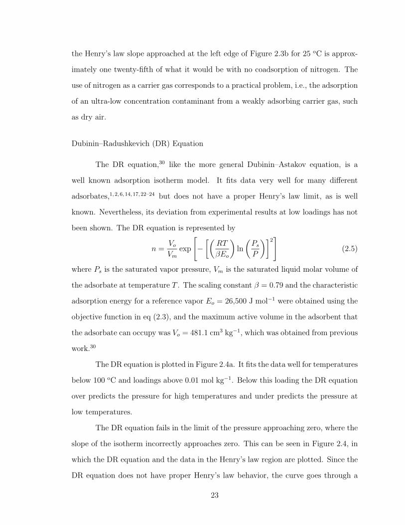
Dubinin–Radushkevich (DR) Equation

The DR equation,30 like the more general Dubinin–Astakov equation, is a

well known adsorption isotherm model. It fits data very well for many different

adsorbates,1,2, 6, 14,17,22–24 but does not have a proper Henry’s law limit, as is well

known. Nevertheless, its deviation from experimental results at low loadings has not

been shown. The DR equation is represented by

n =Vo

Vm

exp

[−[(

RT

βEo

)ln

(Ps

P

)]2]

(2.5)

where Ps is the saturated vapor pressure, Vm is the saturated liquid molar volume of

the adsorbate at temperature T . The scaling constant β = 0.79 and the characteristic

adsorption energy for a reference vapor Eo = 26,500 J mol−1 were obtained using the

objective function in eq (2.3), and the maximum active volume in the adsorbent that

the adsorbate can occupy was Vo = 481.1 cm3 kg−1, which was obtained from previous

work.30

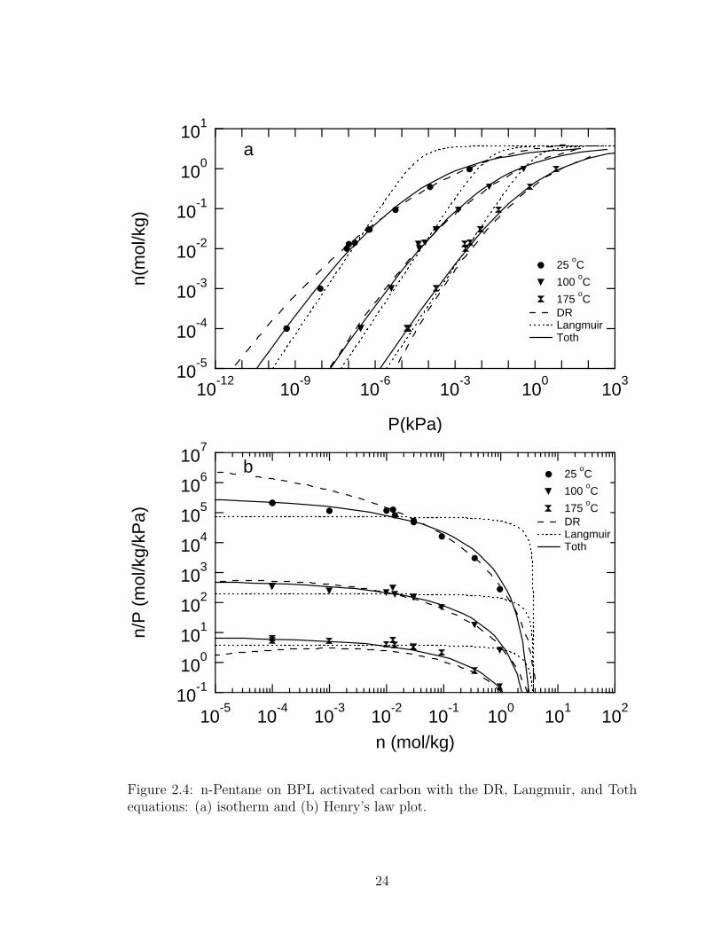
The DR equation is plotted in Figure 2.4a. It fits the data well for temperatures

below 100 oC and loadings above 0.01 mol kg−1. Below this loading the DR equation

over predicts the pressure for high temperatures and under predicts the pressure at

low temperatures.

The DR equation fails in the limit of the pressure approaching zero, where the

slope of the isotherm incorrectly approaches zero. This can be seen in Figure 2.4, in

which the DR equation and the data in the Henry’s law region are plotted. Since the

DR equation does not have proper Henry’s law behavior, the curve goes through a

23

10-5

10-4

10-3

10-2

10-1

100

101n(

mol

/kg)

10-12 10-9 10-6 10-3 100 103

P(kPa)

25 oC 100 oC 175 oC DR Langmuir Toth

a

10-1100101102103104105106107

n/P

(mol

/kg/

kPa)

10-5 10-4 10-3 10-2 10-1 100 101 102

n (mol/kg)

25 oC 100 oC 175 oC DR Langmuir Toth

b

Figure 2.4: n-Pentane on BPL activated carbon with the DR, Langmuir, and Tothequations: (a) isotherm and (b) Henry’s law plot.

24

maximum. This behavior can be seen to shift to higher loadings at higher tempera-

tures, becoming very pronounced at 175 oC and loadings below 0.01 mol kg−1. For

lower temperatures the DR equation has not yet gone through a maximum.

Langmuir Equation

The Langmuir equation was developed for a homogeneous surface, where the

adsorption is localized, but is used more broadly. The equation is31

n =nobP

1 + bP(2.6)

with

b = bo√T exp (Q/RT ) (2.7)

where no is the saturation loading, and Q is the isosteric heat of adsorption at zero

loading. The parameters for the Langmuir equation are given in Table 2.3 and were

obtained using the objective function. The Langmuir equation has a proper Henry’s

law region where the Henry’s constant is KH = nob. The saturation loading for

n-pentane was set to 3.68 mol kg−1 based on previous work.30

The Langmuir equation is plotted with the data in Figure 2.4a. It is readily

apparent that it does not fit the data well. BPL activated carbon is a heterogeneous

material, and the Langmuir equation does not describe the data over the wide range

of the measurements.

The Henry’s law plot for the Langmuir equation is shown in Figure 2.4b. The

equation shows the Henry’s law region being entered at all temperatures near 1 mol

kg−1, based on the parameters regressed from the objective function. However, there

is wide disagreement with the data.

25

Toth Equation

The Toth equation is a well known isotherm equation that was developed for

heterogeneous materials. We use the multi-temperature Toth equation32 in the form

n =nsbP

[1 + (bP )t](1/t)(2.8)

where the saturation loading is

ns = no exp [χ(1− T/To)] (2.9)

with

b = bo exp (Q/RT ) (2.10)

and

t = to + α(1− To/T ) (2.11)

with To = 298.15 K. The Toth equation, like the Langmuir equation, has a proper

Henry’s law limit and a finite saturation loading. The parameters obtained by regres-

sion are shown in Table 2.3. The saturation loading was fixed at 3.68 mol kg−1 for

the same reason as described for the Langmuir equation. The saturation loading is a

very weak function of temperature, and the parameters b and t are strong functions

of temperature.

The Toth equation is shown with all of the data in Figure 2.3 where it fits

the data reasonably well over a wide range of loadings and temperatures. Figure 2.4

shows the Toth equation in comparison with the DR and Langmuir equations. The

Toth equation overcomes the shortcomings of the DR and Langmuir equations for

this system – a proper Henry’s law slope and the transition from Henry’s law toward

non-linear adsorption, respectively. For all temperatures, the Toth equation enters

the Henry’s law region at loadings near 0.01 mol kg−1.

The measured isotherms were used to calculated the isosteric heat of adsorp-

26

tion using the thermodynamic relationship

∆Ha = −R ∂ lnP

∂(1/T )

∣∣∣∣n

(2.12)

Figure 2.5 shows lnP plotted versus 1/T at constant n with the Toth equation and

the vapor pressure of n-pentane. The values of the isosteric heat for specific loadings

are shown in Table 2.4, where the values have been assumed to be independent of

temperature.

27

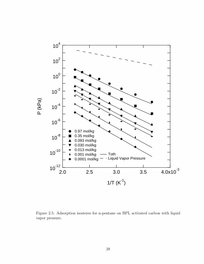
10-12

10-10

10-8

10-6

10-4

10-2

100

102

104P

(kP

a)

4.0x10-33.53.02.52.0

1/T (K-1)

0.97 mol/kg 0.35 mol/kg 0.093 mol/kg 0.030 mol/kg 0.013 mol/kg 0.001 mol/kg 0.0001 mol/kg

Toth Liquid Vapor Pressure

Figure 2.5: Adsorption isosteres for n-pentane on BPL activated carbon with liquidvapor pressure.

28

Table 2.3: Model parameters for the Langmuir and Toth equations

no χ bo Q to α( mol/kg) (kPa)−1 (kJ mol−1)

Langmuir 3.68 1.00 ×10−10 74.5Toth 3.68 9.0×10−11 8.85×10−10 80.2 0.217 0.205

Table 2.4: Calculated isosteric heats of adsorption

Loading ( mol kg−1) ∆Ha ( kJ mol−1)0.97 59.70.35 66.50.093 69.90.030 72.10.013 73.30.001 74.10.0001 77.3

29

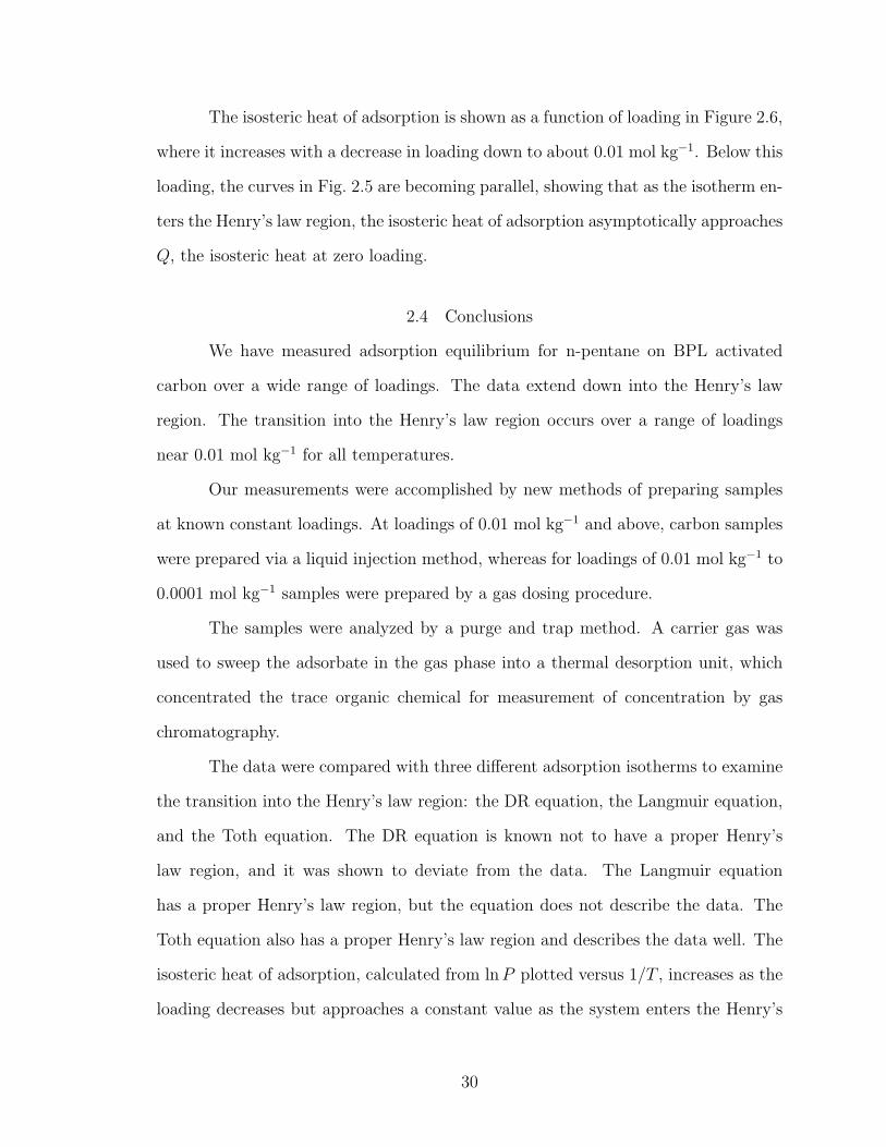
The isosteric heat of adsorption is shown as a function of loading in Figure 2.6,

where it increases with a decrease in loading down to about 0.01 mol kg−1. Below this

loading, the curves in Fig. 2.5 are becoming parallel, showing that as the isotherm en-

ters the Henry’s law region, the isosteric heat of adsorption asymptotically approaches

Q, the isosteric heat at zero loading.

2.4 Conclusions

We have measured adsorption equilibrium for n-pentane on BPL activated

carbon over a wide range of loadings. The data extend down into the Henry’s law

region. The transition into the Henry’s law region occurs over a range of loadings

near 0.01 mol kg−1 for all temperatures.

Our measurements were accomplished by new methods of preparing samples

at known constant loadings. At loadings of 0.01 mol kg−1 and above, carbon samples

were prepared via a liquid injection method, whereas for loadings of 0.01 mol kg−1 to

0.0001 mol kg−1 samples were prepared by a gas dosing procedure.

The samples were analyzed by a purge and trap method. A carrier gas was

used to sweep the adsorbate in the gas phase into a thermal desorption unit, which

concentrated the trace organic chemical for measurement of concentration by gas

chromatography.

The data were compared with three different adsorption isotherms to examine

the transition into the Henry’s law region: the DR equation, the Langmuir equation,

and the Toth equation. The DR equation is known not to have a proper Henry’s

law region, and it was shown to deviate from the data. The Langmuir equation

has a proper Henry’s law region, but the equation does not describe the data. The

Toth equation also has a proper Henry’s law region and describes the data well. The

isosteric heat of adsorption, calculated from lnP plotted versus 1/T , increases as the

loading decreases but approaches a constant value as the system enters the Henry’s

30

85

80

75

70

65

60

55

∆Ha

(kJ/

mol

)

1.00.80.60.40.20.0

n (mol/kg)

Figure 2.6: Isosteric heat of adsorption vs. loading. These can be compared with theheat of vaporization of 25.79 kJ mol−1 for n-pentane at the normal boiling point.33

31

law region.

32

References

[1] Foster KL, Fuerman RG, Economy J, Larson SM, Rood MJ. Adsorption Char-

acteristics of Trace Volatile Organic Compounds in Gas Streams onto Activated

Carbon Fibers. Chem. Mater. 1992; 4:1068–1073

[2] Pinto ML, Pires J, Carvalho AP, de Carvalho MB. On the Difficulties of Predict-

ing the Adsorption of Volatile Organic Compounds at Low Pressures in Microp-

orous Solid: The Example of Ethyl Benzene. J. Phys. Chem. B 2006; 110:250–257

[3] Kuro-oka M, Suzuki T, Nitta T, Katayama T. Adsorption Isotherms of Hydro-

carbons and Carbon Dioxide on Activated Fiber Carbon. J. Chem. Eng. Japan

1984; 17:588–592

[4] Eissmann RN, LeVan MD. Coadsorption of Hydrocarbons and Water on BPL

Activated Carbon. 2. 1,1,2-Trichloro-1,2,2-trifluoroethane and Dichloromethane.

Ind. Eng. Chem. Res. 1993; 32:2752–2757

[5] Kaul BK. Modern Version of Volumeteric Apparatus for Measuring Gas-Solid

Equilibrium Data. Ind. Eng. Chem. Res. 1987; 26:928–933

[6] Mahle JJ, Buettner LC, Friday DK. Measurement and Correlation of the Ad-

sorption Equilibria of Refrigerant Vapors on Activated Carbon. Ind. Eng. Chem.

Res. 1994; 33:346–354

[7] Russell BP, LeVan MD. Coadsorption of Organic Compounds and Water Vapor

on BPL Activated Carbon. 3. Ethane, Propane, and Mixing Rules. Ind. Eng.

Chem. Res. 1997; 36:2380–2389

[8] Karwacki CJ, Morrison RW. Adsorptive Retention of Volatile Vapors for Non-

destructive Filter Leak Testing. Ind. Eng. Chem. Res. 1998; 37:3470–3480

33

[9] Pigorini, G. Periodic Behavior of Pressure Swing Adsorption Cycles and Coad-

sorption of Light and Heavy n–alkanes on Activated Carbon. Charlottsville VA

USA, University of Virginia, PhD thesis, 2000

[10] Walton KS, Pigorini G, LeVan MD. Simple Group-Contribution Theory for Ad-

sorption of Gases and Gas Mixtures in Nanoporous Carbons. Chem. Eng. Sci.

2004; 59:4425–4432

[11] LeVan MD, Pigorini G. Group-Contribution Theory for Coadsorption of Gases

and Vapors on Solid Surfaces. Proceedings of the First International Conference

on Molecular Modeling and Simulation, Keystone, Colorado; Cummings, P. T.,

Westmoreland, P. R., Eds.; 2001, 296–299

[12] Zhu W, Groen JC, Kapteijn F, Moulijn JA. Adsorption of Butane Isomers and

SF6 on Kureha Activated Carbon: 1. Equilibrium. Langmuir 2004; 20:5277–5284

[13] Zhu W, Groen JC, van Miltenburg A, Kapteijn F, Moulijn JA. Comparison of

Adsorption Behavior of Light Alkanes and Alkenes on Kureha Activated Carbon.

Carbon 2005; 43:1416–1423

[14] Golden TC, Kumar R. Adsorption Equilibrium and Kinetics for Multiple Trace

Impurities in Various Gas Streams on Activated Carbon. Ind. Eng. Chem. Res.

1993; 32:159–165

[15] Do HD, Do DD. Structural Heterogeneity in the Equilibrium Data for Hydrocar-

bons and Carbon Oxides on Activated Carbons. Gas Separation & Purification

1994; 8:77–93

[16] Rudisill NR, Hacskaylo JJ, LeVan MD. Coadsorption of Hydrocarbons and Water

on BPL Activated Carbon. Ind. Eng. Chem. Res. 1992; 31:1122–1130

34

[17] Yun JH, Hwang KY, Choi DK. Adsorption of Benzene and Toluene Vapors on

Activated Carbon Fiber at 298, 323, and 348 K. J. Chem. Eng. Data 1998;

43:843–845

[18] Taqvi SM, Appel AS, LeVan MD. Coadsorption of Organic Compounds and

Water Vapor on BPL Activated Carbon. 4. Methanol, Ethanol, Butanol, and

Modeling. Ind. Eng. Chem. Res. 1997; 36:2380–2389

[19] Qi N, LeVan MD. Coadsorption of Organic Compounds and Water Vapor on BPL

Activated Carbon. 5. Methyl Ethyl Ketone, Methyl Isobutyl Ketone, Toluene,

and Modeling. Ind. Eng. Chem. Res. 1997; 36:2380–2389

[20] Yang RT, Long RQ, Padin J, Takahashi A, Takahashi T. Adsorbents of Dioxins:

A New Technique for Sorbent Screening for Low-Volatile Organics. Ind. Eng.

Chem. Res. 1999; 38:2726–2731

[21] Mayfield PLJ, Do DD. Measurement of the Single-Component Adsorption Kinet-

ics of Ethane, Butane, and Pentane onto Activated Carbon Using a Differential

Adsorption Bed. Ind. Eng. Chem. Res. 1991; 30:1262–1270

[22] Linders MJG, Van Den Broeke LJP, Van Bokhoven JJGM, Duisterwinkel AE,

Kapteijn F, Moulijn JA. Effect of the Adsorption Iostherm on One-and Two-

Component Diffusion in Activated Carbon. Carbon 1997; 35:1415–1425

[23] Himeno S, Urano K. Measurement and Correlation of Single and Binary Gas Ad-

sorption Equilibria of Volatile Organic Compounds in Trace Concentrations us-

ing Headspace Gas Chromatography Method. Kagaku Kogaku Ronbunshu 2003;

29:653–659

[24] Himeno S, Kohei U. Determination and Correlation of Binary Gas Adsorption

Equilibria of VOCs. J. of Environ. Eng. 2006; 132:301–308

35

[25] Karwacki CJ, Buettner LC, Buchanan JH, Mahle JJ, Tevault DE. Low-

Concentration Adsorption Studies for Low-Volatility Vapors. Fundamentals of

Adsorption. Meunier, F.; Ed.; Elsevier: Amsterdam, The Netherlands, 1998:

315–320

[26] Karwacki CJ, Tevault DE, Mahle JJ, Buchnan JH, Buettner LC. Adsorption of

Equilibria of Isopropyl Methylphosphonofluoridate (GB) on Activated Carbon

at Ultralow Relative Pressures. Langmuir 1999; 15:6343–6345

[27] LeVan MD, Carta G.(2008). Section 16: Adsorption and Ion Exchange. In:

Green, DW (Ed.) Perry’s Chemical Engineers’ Handbook, 8th ed., McGraw-Hill,

New York, 16.31–32

[28] Myers AL, Prausnitz JM. Thermodynamics of mixed-gas adsorption. AIChE J.

1965; 11:121–127

[29] Meredith MM, Plank CA. Adsorption of Carbon Dioxide and Nitrogen on Char-

coal at 30o and 50 oC. J. Chem. Eng. Data 1967; 12:259–261

[30] Ye XH, Qi N, Ding YQ, LeVan MD. Prediction of Adsorption Equilibrium using

a Modified D-R Equation: Pure Organic Compounds on BPL Carbon. Carbon

2003; 41:681–686

[31] De Boer JH. The Dynamical Character of Adsorption, 2nd ed. Oxford: Claren-

don Press; 1970

[32] Do DD. Adsorption Analysis: Equilbria and Kinetics. London: Imperial College

Press; 1998

[33] Poling BE, Prausnitz JM, O’Connell JP. The Properties of Gases and Liquids.

5th ed. New York:McGraw-Hill;2001

36

CHAPTER III

THE THEORETICAL MAXIMUM ISOSTERIC HEAT OF ADSORPTION IN

THE HENRY’S LAW REGION FOR SLIT-SHAPED CARBON NANOPORES

3.1 Introduction

The isosteric heat of adsorption can yield important information about the

mechanism and properties of adsorption. This is especially true for the isosteric heat

of adsorption in the Henry’s law region, qost. From this we can determine the pore

size to which the molecules are most strongly attracted.

The Henry’s law region for adsorption equilibria is the low-loading region where

the isotherm becomes linear. In this regime, each gas molecule can explore the whole

adsorbent surface independently, as adsorbate-adsorbate molecule interactions are

negligible because of low densities. In the Henry’s law region, the gases in the fluid

phase will be most strongly attracted to the adsorption sites with the highest energies.

However, for a heterogeneous adsorbent, even in the Henry’s law region, adsorption

will occur over a range of pore sizes, although the distribution will be narrower than

at higher pressures. This means that if a material had a single pore size equal to

the pore width where qost is a maximum, the qo

st calculated would be equal to the

maximum theoretical value.

Knowledge of the isosteric heat of adsorption for a molecule as a function of the

pore width can help in the design of new materials. It is important in many ongoing

efforts to create new synthetic carbonaceous materials such as carbon nanotubes,

carbon fibers, metal organic frameworks, and carbon-silica composites. Specifically,

it is important to know the pore widths that would be desirable or undesirable for the

material, as determined from the process for which the materials are being designed.

For some applications, such as air filters, an adsorbent material with a high heat of

adsorption would be desired to provide as strong a hold on contaminant molecules

37

as possible. For gas storage applications, knowing the maximum isosteric heat of

adsorption will help screen potential materials for the application.1,2 For example,

Bhatia and Myers2 have calculated that for hydrogen storage on carbon materials, if

the system is run between pressures of 1.5 bar and 30 bar, a change in the isosteric

heat of adsorption of 15.1 kJ/mol is needed for optimum delivery. In contrast, in

a pressure swing adsorption process, a lower isosteric heat of adsorption would be

desired to reduce the thermal swings in the process and allow for a more efficient

regeneration.

Steele3 developed an equation to calculate qost using statistical thermodynam-

ics. Steele’s equation has been applied by Vernov and Steele4 to calculate qost for

benzene adsorbed on graphite. Pikunic et al. 5 also used the equation to calculate qost

for nitrogen adsorbed on graphitic carbon at different temperatures. Do et al. 6 used

Henry’s constants to fit the solid-fluid attractive potential for various gases at differ-

ent temperatures and also calculated qost. Pan et al. 7 calculated the isosteric heat

of adsorption for propane and butane using density functional theory for a variety of

loadings, temperatures, and pore sizes; qost was calculated as a function of pore width,

which shows a sharp increase for small pores, but a maximum was not found. Floess

and VanLishout8 calculated qost for argon as a function of pore width. A maximum was

found at 6.8 A by integrating the Lennard-Jones 6-12 potential over 3 layers of carbon

to form the pore walls. In this paper qost is calculated as a function of the pore width

for nitrogen, argon, carbon dioxide, methane, helium, and hydrogen. We determine

where qost is a maximum and also where it is equal to zero. We show general results

of the pore width where qost is a maximum as a function of the solid-fluid collision

diameter σsf and the solid-fluid well depth potential εsf . The theoretical values are

compared with qost calculated from adsorption isotherms for nitrogen, argon, carbon

dioxide, and methane on various activated carbons. Results for helium and hydrogen

are not compared with experimental results due to a lack of reliable data.

38

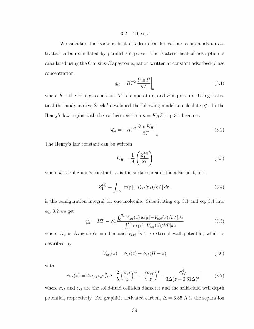
3.2 Theory

We calculate the isosteric heat of adsorption for various compounds on ac-

tivated carbon simulated by parallel slit pores. The isosteric heat of adsorption is

calculated using the Clausius-Clapeyron equation written at constant adsorbed-phase

concentration

qst = RT 2 ∂ lnP

∂T

∣∣∣∣n

(3.1)

where R is the ideal gas constant, T is temperature, and P is pressure. Using statis-

tical thermodynamics, Steele3 developed the following model to calculate qost. In the

Henry’s law region with the isotherm written n = KHP , eq. 3.1 becomes

qost = −RT 2 ∂ lnKH

∂T

∣∣∣∣n

(3.2)

The Henry’s law constant can be written

KH =1

A

(Z

(s)1

kT

)(3.3)

where k is Boltzman’s constant, A is the surface area of the adsorbent, and

Z(s)1 =

∫V (s)

exp [−Vext(r1)/kT ] dr1 (3.4)

is the configuration integral for one molecule. Substituting eq. 3.3 and eq. 3.4 into

eq. 3.2 we get

qost = RT −Na

∫ Hc

0Vext(z) exp [−Vext(z)/kT ]dz∫ Hc

0exp [−Vext(z)/kT ]dz

(3.5)

where Na is Avagadro’s number and Vext is the external wall potential, which is

described by

Vext(z) = φsf (z) + φsf (H − z) (3.6)

with

φsf (z) = 2πεsfρsσ2sf∆

[2

5

(σsf

z

)10

−(σsf

z

)4

−σ4

sf

3∆(z + 0.61∆)3

](3.7)

where σsf and εsf are the solid-fluid collision diameter and the solid-fluid well depth

potential, respectively. For graphitic activated carbon, ∆ = 3.35 A is the separation

39

between the graphite planes and ρs = 0.114 A−3 is the density of the solid.18 Steele3

derived eq. 3.7 because integrating a Lennard-Jones 6-12 potential over just a few

layers of adsorbent did not give good results. The pore width Hc is the distance

between the center of the carbon atoms on opposing walls of the pore, and the pore

width H = Hc− σss is the shortest distance between the surface of the carbon atoms

on opposing walls, where σss = 3.38 A is the size of a carbon atom. See Figure 3.1

for a diagram of the pore.

3.3 Results

We examine qost for six different molecules: nitrogen, argon, methane, carbon

dioxide, helium, and hydrogen. The parameters used to describe these molecules

are given in Table 3.1, with all calculations done at T = 298.15 K. The fluid-fluid

parameters are included for comparison, but were not used in calculating qost because

fluid-fluid molecule interactions are negligible in the adsorbed phase in the Henry’s

law regime. The solid-fluid parameters for all molecules except hydrogen were found

in the literature. The solid-fluid parameters were calculated for hydrogen using the

Lorentz-Berthelot combining rules

σsf = (σff + σss)/2 and εsf =√εffεss (3.8)

where εss/k = 27.97 K. We consider the isosteric heat of adsorption for the six selected

molecules to determine where the isosteric heat of adsorption reaches a maximum

value and also where the isosteric heat of adsorption is equal to zero.

40

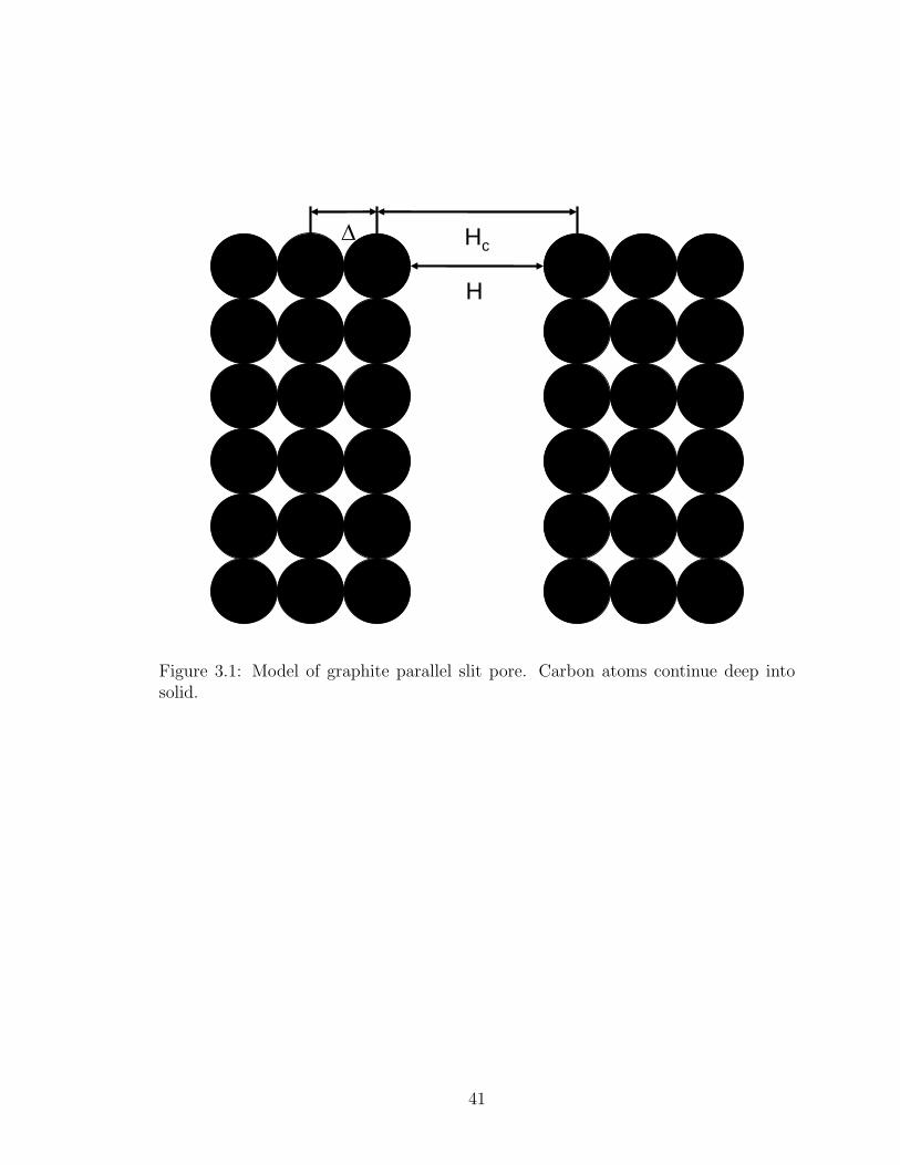
Hc∆

H

Figure 1: Model of graphite parallel slit pore. Carbon atoms

continue deep into solid.

Figure 3.1: Model of graphite parallel slit pore. Carbon atoms continue deep intosolid.

41

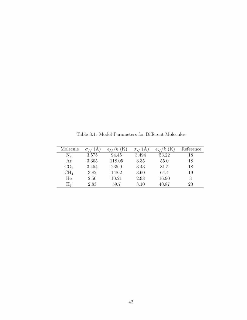
Table 3.1: Model Parameters for Different Molecules

Molecule σff (A) εff/k (K) σsf (A) εsf/k (K) ReferenceN2 3.575 94.45 3.494 53.22 18Ar 3.305 118.05 3.35 55.0 18

CO2 3.454 235.9 3.43 81.5 18CH4 3.82 148.2 3.60 64.4 19He 2.56 10.21 2.98 16.90 3H2 2.83 59.7 3.10 40.87 20

42

We also compare the maximum value of qost determined from eq. 3.5 with qo

st

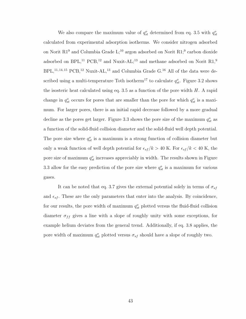
calculated from experimental adsorption isotherms. We consider nitrogen adsorbed

on Norit R19 and Columbia Grade L;10 argon adsorbed on Norit R1;9 carbon dioxide

adsorbed on BPL,11 PCB,12 and Nuxit-AL;13 and methane adsorbed on Norit R1,9

BPL,11,14,15 PCB,12 Nuxit-AL,13 and Columbia Grade G.16 All of the data were de-

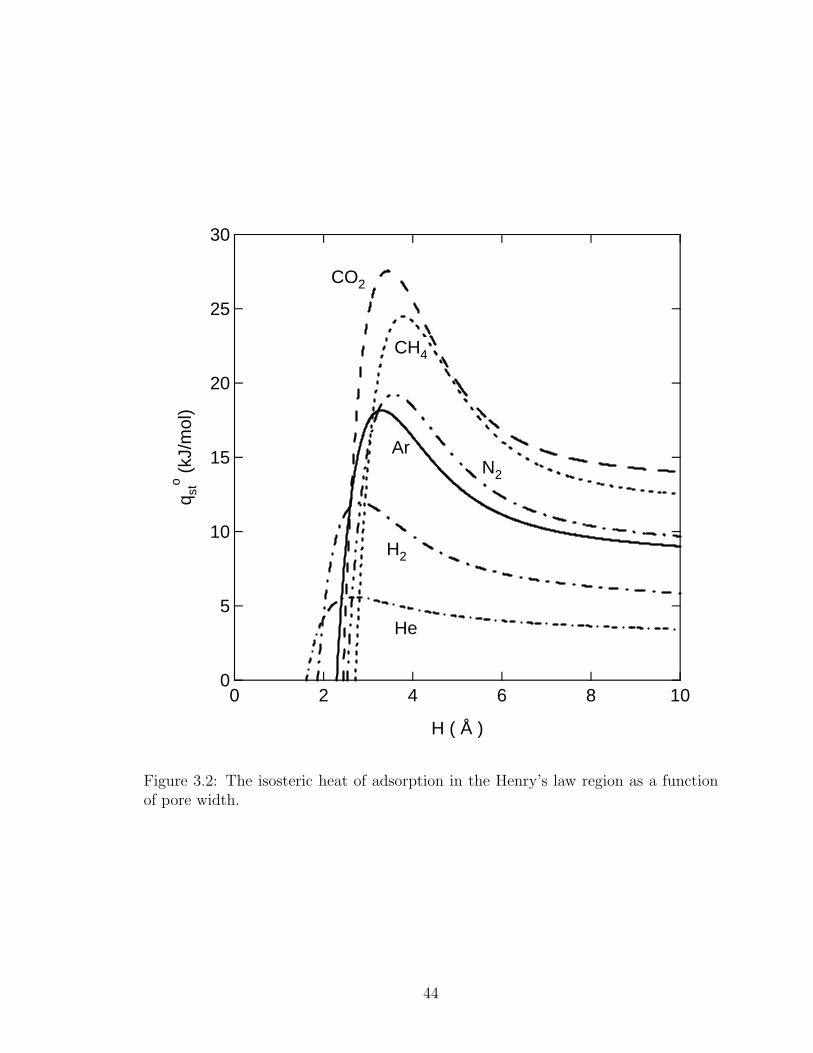
scribed using a multi-temperature Toth isotherm17 to calculate qost. Figure 3.2 shows

the isosteric heat calculated using eq. 3.5 as a function of the pore width H. A rapid

change in qost occurs for pores that are smaller than the pore for which qo

st is a maxi-

mum. For larger pores, there is an initial rapid decrease followed by a more gradual

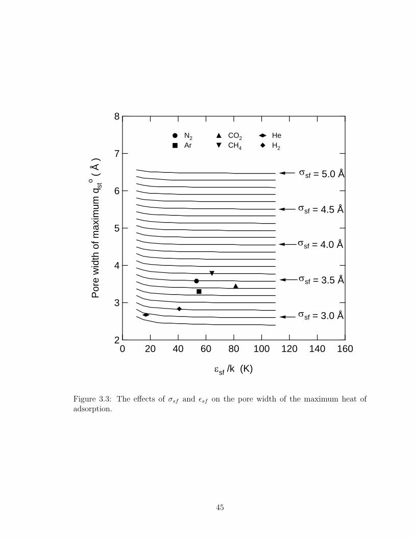
decline as the pores get larger. Figure 3.3 shows the pore size of the maximum qost as

a function of the solid-fluid collision diameter and the solid-fluid well depth potential.

The pore size where qost is a maximum is a strong function of collision diameter but

only a weak function of well depth potential for εsf/k > 40 K. For εsf/k < 40 K, the

pore size of maximum qost increases appreciably in width. The results shown in Figure

3.3 allow for the easy prediction of the pore size where qost is a maximum for various

gases.

It can be noted that eq. 3.7 gives the external potential solely in terms of σsf

and εsf . These are the only parameters that enter into the analysis. By coincidence,

for our results, the pore width of maximum qost plotted versus the fluid-fluid collision

diameter σff gives a line with a slope of roughly unity with some exceptions, for

example helium deviates from the general trend. Additionally, if eq. 3.8 applies, the

pore width of maximum qost plotted versus σsf should have a slope of roughly two.

43

30

25

20

15

10

5

0

q sto (k

J/m

ol)

1086420

H ( Å )

CO2

CH4

N2

Ar

He

H2

Figure 2: The isosteric heat of adsorption in the Henry's law region as a function of pore width.

Figure 3.2: The isosteric heat of adsorption in the Henry’s law region as a functionof pore width.

44

8

7

6

5

4

3

2

Por

e w

idth

of m

axim

um q

sto (

Å )

160140120100806040200

εsf /k (K)

σsf = 3.0 Å

σsf = 3.5 Å

σsf = 4.0 Å

N2 CO2 He Ar CH4 H2

σsf = 4.5 Å

σsf = 5.0 Å

Figure 3: The effects of σsf and εsf on the pore width of the maximum heat of adsorption.

Figure 3.3: The effects of σsf and εsf on the pore width of the maximum heat ofadsorption.

45

Table 3.2: Isosteric Heat of Adsorption in the Henry’s Law Region

Molecule Pore width of Pore width of Maximum qost from Reference

maximum qost zero qo

st qost data

H (A) H (A) (kJ/mol) (kJ/mol)N2 3.58 2.53 19.23 16.64 9

15.92 10Ar 3.30 2.29 18.16 15.22 9

CO2 3.45 2.43 27.55 21.38 1120.55 1223.77 13

CH4 3.78 2.71 24.47 15.80 919.30 1120.29 1220.34 1318.33 1420.88 1516.26 16

He 2.67 1.61 5.58H2 2.83 1.87 11.93

46

For argon the maximum value of qost occurs in a pore of width 3.30 A, which

is much smaller than the value calculated by Floess and VanLishout8 of 6.8 A. Most

of this difference in pore size can be attributed to the differences in the way the pore

size is calculated. The pore size of Floess and VanLishout8 is equivalent to Hc in

this paper, the distance from the center of the carbon atoms on opposing sides of

the slit pore. If the value of the pore size is changed from Hc to H, the actual slit

width between the carbon atoms, the pore size of Floess and VanLishout8 becomes

3.42 A. The remaining differences can be attributed to different external potentials

and different parameters.

Also of interest is the pore size where qost is equal to zero. This point is

interesting because the molecules will not adsorb appreciably and adsorption begins

to become thermodynamically unfavorable. These pore widths, given in Table 3.2,

are smaller than σsf and correspond roughly to pores for which the external potential

is zero at the center, indicating a balance between attractive and repulsive effects. qost

is equal to zero for argon in a pore of width 2.29 A. If the same procedure is applied

to the pore width for which qost is equal to zero as was applied to the pore width of

the maximum qost, the value of Floess and VanLishout8 changes from 5.8 A to 2.42 A.

The results obtained from eq. 3.5 are compared with qost calculated from ad-

sorption isotherms9–16 in Table 3.2. The values calculated using eq. 3.5 are 15%–55%

higher than the values calculated from the adsorption data. These differences can be

attributed to the pore size distribution. Even though the isotherm is in the Henry’s

law region, adsorption occurs in a range of pore sizes. The pore size range will be

narrower in the Henry’s law region than at higher pressures because the molecules will

be exposed to a higher percentage of the adsorption sites with the highest energies.

As the pressure increases, because of the energy distribution of adsorption sites and

higher loadings, the molecules will fill a broader range of pore sizes including those

with lower energies.

47

The value of the maximum qost is important for the design of new materials

for processes such as adsorptive storage. As mentioned earlier, Bhatia and Myers2

calculated the change in the heat of adsorption between two pressures that is needed

to reach the Department of Energy’s goals for hydrogen21 and the 180 v/v goal for

methane. For hydrogen, adsorbed on carbon materials between the pressures of 1.5

bar and 30 bar at 298 K, the change in the heat of adsorption needs to be 15.1 kJ/mol

for optimal delivery. This change in the isosteric heat of adsorption is higher than the

maximum qost for hydrogen of 11.93 kJ/mol, which occurs in a pore of width 2.83 A.

Also, the optimal value for methane is equal to 18.8 kJ/mol at the same conditions,

which is lower than the maximum value of 24.47 kJ/mol, which we found in a pore

of width 3.78 A. This agrees with the conclusion of Bhatia and Myers2 that carbon

materials will not be acceptable for hydrogen storage at ambient temperatures. How-

ever, methane could reach the Department of Energy’s goal with properly designed

materials.

3.4 Conclusions

In this paper we have calculated qost as a function of pore width for nitro-

gen, argon, carbon dioxide, methane, helium, and hydrogen. We have compared the

maximum value calculated from eq. 3.5 with the isosteric heat calculated from data

adsorbed on various activated carbons. The calculated theoretical maximum was

15%–55% higher than the values calculated from the adsorption isotherms.

The pore size where qost is a maximum was calculated as a general function

of the collision diameter and the well depth potential, thus allowing for the easy

prediction of the pore size where qost is a maximum for molecules not discussed in

this paper. We have demonstrated that the pore where qost is a maximum is a strong

function of the collision diameter and a weak function of the well depth potential

when εsf/k is greater than 40 K. We have shown that under the conditions set forth

48

by Bhatia and Myers2 for adsorptive storage, carbon materials will not be suitable

for hydrogen but could be acceptable for methane if designed correctly.

49

References

[1] Gigras A, Bhatia SK, Anil Kumar AV, Myers AL. Feasibility of tailoring for high

isosteric heat to improve effectiveness of hydrogen storage in carbons. Carbon

2007;45:1043–50.

[2] Bhatia SK, Myers AL. Optimum Conditions for Adsorptive Storage. Langmuir

2006;22:1688–1700.

[3] Steele WA. The Interaction of Gases with Solid Surfaces. Oxford:Pergamon

Press;1974.

[4] Vernov A, Steele WA. Computer Simulations of Benzene Adsorbed on Graphite.

1. Langmuir 1991;7:3110–17.

[5] Pikunic J, Clinard C, Cohaut N, Gubbins KE, Guet J, Pellenq JM, et al. Struc-

tural Modeling of Porous Carbons: Constrained Reverse Monte Carlo Method.

Langmuir 2003;19:8565–82.

[6] Do DD, Do HD, Tran KN. Analysis of Adsorption of Gases and Vapors on

Nonporous Graphatized Thermal Carbon Black. Langmuir 2003;19:5656–68.

[7] Pan H, Ritter JA, Balbuena PB. Isosteric Heats of Adsorption on Carbon Pre-

dicted by Density Functional Theory. Ind. Eng. Chem. Res. 1998;37:1159–66.

[8] Floess JK, VanLishout Y. Calculation of Adsorption Energies in Carbon Micro-

pores. Carbon 1992;30:967–73.

[9] Herbst A, Harting P. Thermodynamic Description of Excess Isotherms in High-

Pressure Adsorption of Methane, Argon, and Nitrogen. Adsorption 2002;8:111–

23.

50

[10] Ray GC, Box EO. Adsorption of Gases on Activated Charcoal. Ind. Eng. Chem.

1950;42:1315–18.

[11] Reich R, Ziegler WT, Rogers KA. Adsorption of Methane, Ethane, and Ethylene

Gases and Their Binary and Ternary Mixtures and Carbon Dioxide on Activated

Carbon at 212 – 301 K and Pressures to 35 Atmospheres. Ind. Eng. Chem.

Process Des. Dev. 1980;19:336–44.

[12] Ritter JA, Yang RT. Equilibrium Adsorption of Multicomponent Gas Mixtures

at Elevated Pressures. Ind. Eng. Chem. Res. 1987;26:1679–86.

[13] Szepesy L, Illes V. Adsorption of Gases and Gas Mixtures I. Acta Chim. Hung.

1963;35:37–51. ,Szepesy L, Illes V. Adsorption of Gases and Gas Mixtures II.

Acta Chim. Hung. 1963;35:53–60.

[14] Belmabkhout Y, De Weireld G, Frere M. High-Pressure Adsorption Isotherms

of N2, CH4, O2, and Ar on Different Carbonaceous Adsorbents. J. Chem. Eng.

Data 2004;49:1379–91.

[15] Pigorini G. Periodic Behavior of Pressure Swing Adsorption Cycles and Coad-

sorption of Light and Heavy n-Alkanes on Activated Carbon. Charlottesville VA

USA, University of Virginia, Ph.D. thesis, 2000.

[16] Payne HK, Studervant GA, Leland TW. Improved Two-Dimensional Equation of

State to Predict Adsorption of Pure and Mixed Hydrocarbons. Ind. Eng. Chem.

Fundam. 1968;7:363–74.

[17] Do DD. Adsorption Analysis: Equilbria and Kinetics. London:Imperial College

Press;1998.

51

[18] Ravikovitch PI, Nishnyakov A, Russo R, Neimark AV. Unified Approach to Pore

Size Characterization of Microporous Carbonaceous Materials for N2, Ar, and

CO2, Adsorption Isotherms. Langmuir 2000;16:2311–20.

[19] Ravikovitch PI, Nishnyakov A, Neimark AV. Density functional theories and

molecular simulations of adsorption and phase transitions in nanopores. Physical

Review E 2001;64:Art. No. 011602.

[20] Poling BE, Prausnitz JM, O’Connell JP. The Properties of Gases and Liquids.

5th ed. New York:McGraw-Hill;2001.

[21] DOE Hydrogen Program. 2006 Annual Program Report; Department of Energy;

2006. p. 273–279.

52

CHAPTER IV

MODELING ADSORPTION OF NITROGEN AND PENTANE ON ACTIVATED

CARBON USING SAFT-DFT

4.1 Introduction

The introduction of density functional theory (DFT) to model inhomogeneous

fluids represents a significant advance in fluid theory. The development of DFT was

encouraged by the desire to accurately model phase transitions and has been used

successfully to simulate the adsorption of spherical molecules and the vapor-liquid

phase transition.1,2 DFT was developed with the desire to model systems at the

molecular level with fundamental parameters which include those needed to model

the bulk fluid, the monolayer transition of the adsorbate on a sheet of graphite, and

the pore size distribution(PSD) of the adsorbent.

Tarazona3,4 developed a weighted density approximation for spherical molecules.

A power series expansion in density was used to describe the direct correlation func-

tion. Although this method does not have a solid foundation in theory, it has been

successfully applied to many situations.5–19

Another theory called Fundamental Measure Theory (FMT) was developed by

Rosenfeld20,21 and later improved by Roth et al.22 as an extension of scaled particle

theory for an inhomogeneous fluid. FMT uses simple geometric definitions to describe

a series of densities that when combined correctly describe the direct correlation

function. FMT has been used for a variety of applications.11,23–26 A review of the

development of DFT, both weighted density approximation and FMT, for spherical

molecules is available.27

Pioneering work by Wertheim28–31 on thermodynamic perturbation theory has

led to the development of statistical associating fluid theory (SAFT). Much research

has been performed on SAFT as an equation of state, and reviews are available.32,33

53

There have been many systems studied including alkanes of low molecular weight

through simple polymers34–38 and their binary mixtures,39–48 perfluoroalkanes,49–51

boron triflouride,52 water,53,54 refrigerant systems,55 and carbon dioxide.45,50,56–58

There is much interest in expanding the use of DFT to systems of larger

molecules, such as polymers and chain fluids. There has been an effort to include

SAFT into DFT. The method has split into two distinct ways to calculate the grand

potential. A method first proposed by Chandler et al.59–61 uses a density expansion

approach similar to integral equations. The second method is an extension of FMT.

There have been a number of different ways that this was done, such as by Wood-

ward,62,63 Liu,64,65 Chapman,66–68 and Wu.69–71 Yu and Wu70 used FMT as a basis

for a hard sphere chain fluid. Chapman66 added terms for a first order attractive

potential with a mean field approximation.

In this paper, we extend the theory of Yu and Wu70 for adsorption in slit-

shaped pores. We develop DFT for chain fluids with a first-order non-mean field

approximation and second-order attractive perturbation term. Along the way we

compare our results with published results of Monte Carlo simulations for hard-sphere

chains near hard walls and chains with attractive potentials in the presence of hard

walls and attractive walls. Then, we use the theory to model the density profiles

of nitrogen in a carbon parallel slit pore. These data are used to calculate a PSD

for BPL activated carbon. Then we will apply the model to pentane adsorption in

the same system. Using the PSD and the pentane density profiles we calculate an

isotherm for pentane.

4.2 Theory

Model

Density functional theory is used to calculate the density profile that minimizes

the grand potential function Ω[ρM(R)], where ρM(R) is the density profile of a chain

54

molecule as a function of segment position R ≡ (r1, r2, · · · , rM) and M is the number

of segments in the chain. This is done by setting the functional derivative with respect

to the density equal to zero. The grand potential is calculated by

Ω[ρM(R)] = F [ρM(R)] +

∫ρM(R)[Vext(R)− µM ]dR (4.1)

where F [ρM(R)] is the Helmholtz free energy, µM is the chemical potential for the

chain molecule calculated by the SAFT equation of state, and Vext(R) is the external

potential.

The Helmholtz free energy is calculated by an ideal term and excess terms.

The excess terms consist of hard sphere repulsion, chain connectivity, and a first and

second order perturbation for the attractive terms. The ideal term is calculated by

Fid = kT

∫ρ(r)

[ln(Λ3ρ(r))− 1

]dr (4.2)

where Λ is the de Broglie wave length. The density ρ(r) is used instead of ρM(R) be-

cause we are solving for the segment density, not the molecular density. The chemical

potential of the ideal term is calculated from

µid = kT ln(ρMΛ3) (4.3)

where ρM is the molecular density, which is equal to M × ρb, where ρb is the segment

density.

The hard sphere repulsive term is calculated by FMT as developed by Rosen-

feld20 and improved upon later by Roth et al.22 for a Mansoori-Carnahan-Starling-

Leland (MCSL) fluid. Using the improved equations for a MCSL fluid, the hard

sphere free energy is written

Fhs = kT

∫Φhs[nα(r′)]dr′ (4.4)

where

Φhs[nα(r)] = −n0 ln(1− n3) +n1n2 − nV 1 · nV 2

1− n3

+

(n32 − 3n2nV 2 · nV 2)(n3 + (1− n3)

2 ln(1− n3))

36πn23(1− n3)2

(4.5)

55

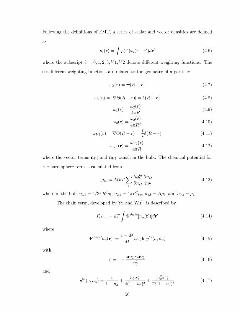
Following the definitions of FMT, a series of scalar and vector densities are defined

as

ni(r) =

∫ρ(r′)ωi(r− r′)dr′ (4.6)

where the subscript i = 0, 1, 2, 3, V 1, V 2 denote different weighting functions. The

six different weighting functions are related to the geometry of a particle:

ω3(r) = Θ(R− r) (4.7)

ω2(r) = |∇Θ(R− r)| = δ(R− r) (4.8)

ω1(r) =ω2(r)

4πR(4.9)

ω0(r) =ω2(r)

4πR2(4.10)

ωV 2(r) = ∇Θ(R− r) =r

rδ(R− r) (4.11)

ωV 1(r) =ωV 2(r)

4πR(4.12)

where the vector terms nV 1 and nV 2 vanish in the bulk. The chemical potential for

the hard sphere term is calculated from

µhs = MkT∑

i

∂φhsb

∂ni,b

∂ni,b

∂ρb

(4.13)

where in the bulk n3,b = 4/3πR3ρb, n2,b = 4πR2ρb, n1,b = Rρb, and n0,b = ρb.

The chain term, developed by Yu and Wu70 is described by

Fchain = kT

∫Φchain[nα(r′)]dr′ (4.14)

where

Φchain[nα(r)] =1−M

Mn0ζ ln yhs(σ, nα) (4.15)

with

ζ = 1− nV 2 · nV 2

n22

(4.16)

and

yhs(σ, nα) =1

1− n3

+n2σζ

4(1− n3)2+

n22σ

2ζ

72(1− n3)3(4.17)

56

The chemical potential for the chain term is described by

µchain = kT (1−M)∑

i

∂φchainb

∂ni

∂ni

∂ρb

(4.18)

For the attractive terms we used a perturbation analysis, neglecting a mean

field assumption, and expanding out to the second order term. The first-order term

is

F1 =1

2

∫ρ(r′)

∫ρ(r′′)ghs[n3(r

′′); r′′]φ(|r′ − r′′|)dr′′dr′ (4.19)

where the attractive potential is a square-well

φ(r;λ) =

−εff if σ ≤ r < λσ0 if r ≥ λσ

(4.20)

and the hard sphere radial distribution function, ghs, developed by Chang and San-

dler72 with a Verlet-Weis73 correction, is a function of distance and density. The

chemical potential for the first-order term is

µ1 = −4Mε(λ3 − 1)

(2n3,bg

hse + n2

3,b

∂ghse

∂ηe

∂ηe

∂n3

)(4.21)

where the hard sphere radial distribution function is calculated by

ghse =

1− ηe/2

(1− ηe)3(4.22)

and the effective density is calculated for an extended value up to λ = 3 using the

relation of Patel et al.74

ηe =c1n3,b + c2n

23,b

(1 + c3n3,b)3(4.23)

with c1c2c3

=

−3.16492 13.35007 −14.80567 5.7028643.00422 −191.66232 273.89683 −128.9333765.04194 −266.46273 361.04309 162.69963

1/λ1/λ2

1/λ3

1/λ4

(4.24)

The second-order term, developed by Zhang,75–77 is a macroscopic compress-

ibility approximation that takes neighboring shells into account. It is given by

F2 = − 1

4kT

∫ρ(r′)

∫ρ(r′′)(1+2ξn2

3)[φ(|r′−r′′|)]2Khs(r′′)ghs[n3(r

′′); r′′]dr′dr′′ (4.25)

57

where ξ = 1/0.4932. The hard sphere isothermal compressibility for a MCSL fluid is

calculated from

Khs =(1− n3)

4

1 + 4n3 + 4n23 − 4n3

3 + n43

(4.26)

with the chemical potential calculated by

µ2 =−2Mε2(λ3 − 1)

kT

[4ξn3

3,bKhsghs

e +(1 + 2ξn2

3,b

)(2n3,bK

hsghse + n2

3,b

[∂Khs

∂n3,b

ghse +Khs∂g

hse

∂ηe

∂ηe

∂n3,b

])] (4.27)

The equation used for the external potential depends on the situation being

described. The interaction between a hard-sphere chain and a hard wall is described

by

Vext(z) =

0, z ≥ 0∞, z < 0

(4.28)

The interaction with a square-well attractive wall is described by

Vext(z) =

0, z > σ−εw, 0 < z < σ∞, z < 0

(4.29)

The carbon wall is described by a 10-4-3 wall78

Vext = φsf (z) + φsf (H − z) (4.30)

where

φsf (z) = 2πεsfρsσ2sf∆

[2

5

(σsf

z

)10

−(σsf

z

)4

−σ4

sf

3∆(z + 0.61∆)3

](4.31)

with ρs = 0.114 A−3 and ∆ = 3.35 A.

Taking the functional derivative of eq. 4.1 and rearranging results in the equa-

tion used to calculate the segment equilibrium density profile

ρ(z) =1

Λ3exp(µ)

M∑i=1

exp

[−ψ(z)

kT

]Gi(z)GM+1−i(z) (4.32)

where M is the number of segments and µ is the chemical potential. The solution

method involves iterating on the segment density. In eq. 4.32, we have

ψ(z) =δFhs

δρ(r)+δFchain

δρ(r)+

δF1

δρ(r)+

δF2

δρ(r)+ Vext (4.33)

58

and

Gi =

∫exp

[−ψ(z)

kT

]Θ(σ − |z − z′|)

2σGi−1dz′ (4.34)

where G1(z) = 1. Due to the summation term in eq. 4.32, the value of the parameter

M is limited to integer values.

The equilibrium value of the density, calculated from eq. 4.32, is then used to

calculate the average excess density in the pore using

ρ(H,P ) =1

H

∫ H

0

[ρ(z)

M− ρb

]dz (4.35)

where ρb is the bulk density, H = Hc − σss is the pore width and Hc is the distance

between the center of the carbon atoms on opposing walls, and σss = 3.38A is the

diameter of the carbon atom. The average excess density is calculated for all pore

widths h and all pressures P .

The PSD of the material is calculated by integrating the average densities

in pores over the range of pore widths and pressures using the adsorption integral

equation

n(Pi) =

∫ h

0

ρ(h, Pi)f(h)dh . . . i = 1, n (4.36)

where ρ(h, Pi) is the average density in the pore and f(h) is the pore size distribution.

The model used for the PSD is a log normal distribution

f(h) =m∑

i=1

αi

γih√

2πexp

[−(ln(h)− βi)

2

2γ2i

](4.37)

where m is the number of modes and αi, βi, and γi are parameters.

Model Validation

As the model was being developed, results were compared with a variety of

different examples in the literature for validation. The model was compared against

a set of hard-sphere chain results against hard-walls. Fig. 4.1 compares the segment

density profiles of the model against a series of Monte Carlo simulations by Kierlik

59

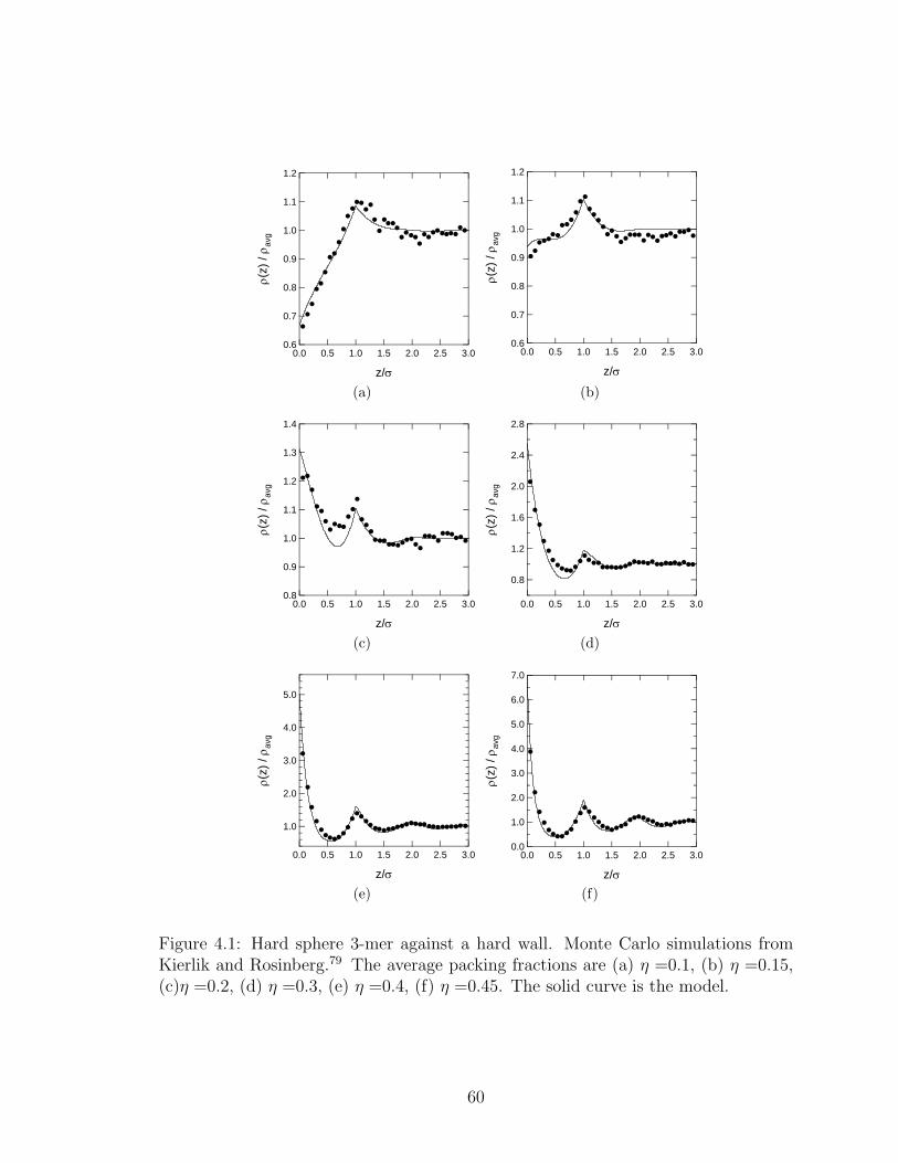
1.2

1.1

1.0

0.9

0.8

0.7

0.6

ρ(z)

/ ρ a

vg

3.02.52.01.51.00.50.0

z/σ

(a)

1.2

1.1

1.0

0.9

0.8

0.7

0.6

ρ(z)

/ ρ a

vg

3.02.52.01.51.00.50.0

z/σ

(b)

1.4

1.3

1.2

1.1

1.0

0.9

0.8

ρ(z)

/ ρ a

vg

3.02.52.01.51.00.50.0

z/σ

(c)

2.8

2.4

2.0

1.6

1.2

0.8

ρ(z)

/ ρ a

vg

3.02.52.01.51.00.50.0

z/σ

(d)

5.0

4.0

3.0

2.0

1.0

ρ(z)

/ ρ a

vg

3.02.52.01.51.00.50.0

z/σ

(e)

7.0

6.0

5.0

4.0

3.0

2.0

1.0

0.0

ρ(z)

/ ρ a

vg

3.02.52.01.51.00.50.0

z/σ(f)

Figure 4.1: Hard sphere 3-mer against a hard wall. Monte Carlo simulations fromKierlik and Rosinberg.79 The average packing fractions are (a) η =0.1, (b) η =0.15,(c)η =0.2, (d) η =0.3, (e) η =0.4, (f) η =0.45. The solid curve is the model.

60

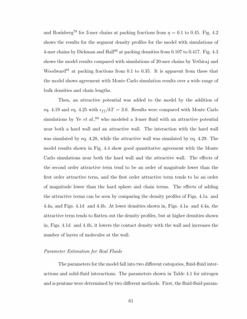
and Rosinberg79 for 3-mer chains at packing fractions from η = 0.1 to 0.45. Fig. 4.2

shows the results for the segment density profiles for the model with simulations of

4-mer chains by Dickman and Hall80 at packing densities from 0.107 to 0.417. Fig. 4.3

shows the model results compared with simulations of 20-mer chains by Yethiraj and

Woodward81 at packing fractions from 0.1 to 0.35. It is apparent from these that

the model shows agreement with Monte Carlo simulation results over a wide range of

bulk densities and chain lengths.

Then, an attractive potential was added to the model by the addition of

eq. 4.19 and eq. 4.25 with εff/kT = 3.0. Results were compared with Monte Carlo

simulations by Ye et al.,64 who modeled a 3-mer fluid with an attractive potential

near both a hard wall and an attractive wall. The interaction with the hard wall

was simulated by eq. 4.28, while the attractive wall was simulated by eq. 4.29. The

model results shown in Fig. 4.4 show good quantitative agreement with the Monte

Carlo simulations near both the hard wall and the attractive wall. The effects of

the second order attractive term tend to be an order of magnitude lower than the

first order attractive term, and the first order attractive term tends to be an order

of magnitude lower than the hard sphere and chain terms. The effects of adding

the attractive terms can be seen by comparing the density profiles of Figs. 4.1a and

4.4a, and Figs. 4.1d and 4.4b. At lower densities shown in, Figs. 4.1a and 4.4a, the

attractive term tends to flatten out the density profiles, but at higher densities shown

in, Figs. 4.1d and 4.4b, it lowers the contact density with the wall and increases the

number of layers of molecules at the wall.

Parameter Estimation for Real Fluids

The parameters for the model fall into two different categories, fluid-fluid inter-

actions and solid-fluid interactions. The parameters shown in Table 4.1 for nitrogen

and n-pentane were determined by two different methods. First, the fluid-fluid param-

61

1.2

1.1

1.0

0.9

0.8

0.7

0.6

ρ(z)

/ ρ a

vg

2.01.51.00.50.0

z/σ

(a)

3.5

3.0

2.5

2.0

1.5

1.0

0.5

0.0

ρ(z)

/ ρ a

vg

2.01.51.00.50.0

z/σ

(b)

6

5

4

3

2

1

0

ρ(z)

/ ρ a

vg

2.01.51.00.50.0

z/σ

(c)

Figure 4.2: Hard sphere 4-mer against a hard wall. Monte Carlo simulations fromDickman and Hall.80 The average packing fractions are (a) η =0.107, (b) η =0.34,(c)η =0.417. The solid curve is the model.

62

0.14

0.12

0.10

0.08

0.06

0.04

0.02

ρ(z)

/ ρ a

vg

3.02.52.01.51.00.50.0

z/σ(a)

0.30

0.25

0.20

0.15

0.10

ρ(z)

/ ρ a

vg

3.02.52.01.51.00.50.0

z/σ(b)

0.6

0.5

0.4

0.3

0.2

ρ(z)

/ ρ a

vg

3.02.52.01.51.00.50.0

z/σ(c)

1.0

0.8

0.6

0.4

0.2

ρ(z)

/ ρ a

vg

3.02.52.01.51.00.50.0

z/σ(d)

Figure 4.3: Hard sphere 20-mer against a hard wall. Monte Carlo simulations fromYethiraj and Woodward.81 The average packing fractions are (a) η =0.1, (b) η =0.2,(c)η =0.3, (d) η = 0.35. The solid curve is the model.

63

1.4

1.2

1.0

0.8

0.6

0.4

0.2

ρ(z)

/ ρ a

vg

43210

z / σff

(a)

1.2

1.1

1.0

0.9

0.8

ρ(z)

/ ρ a

vg

43210

z / σff

(b)

3.0

2.5

2.0

1.5

1.0

0.5

ρ(z)

/ ρ a

vg

43210

z / σff

(c)

3.0

2.5

2.0

1.5

1.0

0.5

ρ(z)

/ ρ a

vg

43210

z / σff

(d)

Figure 4.4: Attractive sphere 3-mer against a hard and attractive wall. Monte Carlosimulations from Ye et al.64 The average packing fractions are (a) η =0.1 hard wall,(b) η =0.3 hard wall, (c) η =0.1 attractive wall, (d) η =0.3 attractive wall. For theattractive wall, the potential between the wall and the fluid is εw/kT = −1.0. Thesolid curve is the model.

64

Table 4.1: Model parameters

molecule σff (A) εff/k (K) λ M σsf (A) εsf/k (K)nitrogen 2.657 40.282 1.83 2 3.0185 42.98

n-pentane 2.791 57.083 2.163 5 3.086 74.63

eters were estimated using the saturated vapor pressure curve and the liquid-vapor

coexistence curve. Then, the solid-fluid parameters were determined by a method

described by Lastoskie et al.5 The solid-fluid molecular diameter σsf was calcu-

lated using the Lorentz-Berthelot mixing rules (arithmetic mean) using the fluid-fluid

molecular diameter σff and the solid molecular diameter σss. The solid-fluid poten-

tial εsf was determined from fitting the onset of the monolayer transition. Results

for parameter estimation will be discussed in the next sections.

4.3 Results

Nitrogen

To estimate the solid-fluid parameters, the process discussed above was used.

For nitrogen, we used data from Kruk et al.82 on Carbopack F, a commercially

available graphitized carbon black with a BET surface area of 6.2 m2/g. A large

pore of half width h = 20 σff was used to simulate a non-porous surface, and the

results are shown in Fig. 4.5. The solid-fluid potential chosen was the value that best

described the curve over the entire range of pressures, up to a reduced pressure of

4×10−3.

Solving eq. 4.32 gives a density profile. In the next few paragraphs we will be

discussing density profiles for three different pore sizes. They will be shown at three

different pressures for each pore size. We will be showing one before the monolayer

transition, one after the monolayer transition but before the freezing transition, and

one after the freezing transition.

65

1.6

1.4

1.2

1.0

0.8

0.6

0.4

0.2

0.0

Vol

ume

adso

rbed

(cc/

g (S

TP))

10-6 10-5 10-4 10-3 10-2

P/Po

Figure 4.5: Comparison of experimental and theoretical adsorbed volumes of nitrogenon nonporous carbon black at 77 K. The points are experimental data. The solid lineis the nitrogen prediction.

66

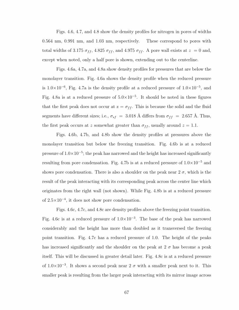
Figs. 4.6, 4.7, and 4.8 show the density profiles for nitrogen in pores of widths

0.564 nm, 0.991 nm, and 1.03 nm, respectively. These correspond to pores with

total widths of 3.175 σff , 4.825 σff , and 4.975 σff . A pore wall exists at z = 0 and,

except when noted, only a half pore is shown, extending out to the centerline.

Figs. 4.6a, 4.7a, and 4.8a show density profiles for pressures that are below the

monolayer transition. Fig. 4.6a shows the density profile when the reduced pressure

is 1.0×10−6, Fig. 4.7a is the density profile at a reduced pressure of 1.0×10−5, and

Fig. 4.8a is at a reduced pressure of 5.0×10−5. It should be noted in these figures

that the first peak does not occur at z = σff . This is because the solid and the fluid

segments have different sizes; i.e., σsf = 3.018 A differs from σff = 2.657 A. Thus,

the first peak occurs at z somewhat greater than σff , usually around z = 1.1.

Figs. 4.6b, 4.7b, and 4.8b show the density profiles at pressures above the

monolayer transition but below the freezing transition. Fig. 4.6b is at a reduced

pressure of 1.0×10−5; the peak has narrowed and the height has increased significantly

resulting from pore condensation. Fig. 4.7b is at a reduced pressure of 1.0×10−5 and

shows pore condensation. There is also a shoulder on the peak near 2 σ, which is the

result of the peak interacting with its corresponding peak across the center line which

originates from the right wall (not shown). While Fig. 4.8b is at a reduced pressure

of 2.5×10−4, it does not show pore condensation.

Figs. 4.6c, 4.7c, and 4.8c are density profiles above the freezing point transition.

Fig. 4.6c is at a reduced pressure of 1.0×10−3. The base of the peak has narrowed

considerably and the height has more than doubled as it transversed the freezing

point transition. Fig. 4.7c has a reduced pressure of 1.0. The height of the peaks

has increased significantly and the shoulder on the peak at 2 σ has become a peak

itself. This will be discussed in greater detail later. Fig. 4.8c is at a reduced pressure

of 1.0×10−3. It shows a second peak near 2 σ with a smaller peak next to it. This

smaller peak is resulting from the larger peak interacting with its mirror image across

67

0.30

0.25

0.20

0.15

0.10

0.05

0.00

ρ(z)

* σ

3 ff

1.20.80.40.0z / σff

h

(a)

20

15

10

5

0

ρ(z)

* σ

3 ff

1.20.80.40.0z / σff

h

(b)

50

40

30

20

10

0

ρ(z)

* σ

3 ff

1.20.80.40.0z / σff

h

(c)

Figure 4.6: Nitrogen density profiles in a 0.564 nm pore, h = 1.575. a) P/Po =1.0×10−6, b) P/Po = 1.0×10−5, c) P/Po = 1.0×10−3.

68

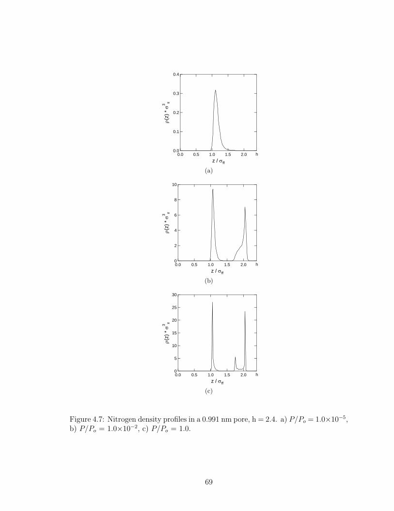
0.4

0.3

0.2

0.1

0.0

ρ(z)

* σ

3 ff

2.01.51.00.50.0z / σff

h

(a)

10

8

6

4

2

0

ρ(z)

* σ

3 ff

2.01.51.00.50.0z / σff

h

(b)

30

25

20

15

10

5

0

ρ(z)

* σ

3 ff

2.01.51.00.50.0z / σff

h

(c)

Figure 4.7: Nitrogen density profiles in a 0.991 nm pore, h = 2.4. a) P/Po = 1.0×10−5,b) P/Po = 1.0×10−2, c) P/Po = 1.0.

69

0.4

0.3

0.2

0.1

0.0

ρ(z)

* σ

3 ff

2.01.51.00.50.0z / σff

h

(a)

3.5

3.0

2.5

2.0

1.5

1.0

0.5

0.0

ρ(z)

* σ

3 ff

2.01.51.00.50.0z / σff

h

(b)

40

30

20

10

0

ρ(z)

* σ

3 ff

2.01.51.00.50.0z / σff

h

(c)

Figure 4.8: Nitrogen density profiles in a 1.03 nm pore, h = 2.475. a) P/Po =5.0×10−5, b) P/Po = 2.5×10−4, c) P/Po = 1.0×10−3.

70

the center line.

Fig. 4.9 shows the density profile of Figs. 4.6c, 4.7c, and 4.8c, but as a full

pore width. This was done to demonstrate the interactions of the larger peaks across

the centerline which results in the smaller peaks. Fig. 4.9a shows the full pore profile

of Fig. 4.6c. It shows two distinct peaks. There are no shoulders, or smaller peaks,

because the two peaks are 1 σ apart. For pores that are slightly off the 0.564 A pore

there is no evidence of the freezing transition. The peak is broader and more diffuse.

Fig. 4.9b is the full pore profile of Fig. 4.7c. The interactions of the large pores in the

center of the pore with the smaller pores becomes easier to see. The large peak at 2

σ and the small peak at 3σ are 1 σ apart, the same is true for the reverse. Fig. 4.9c

is the full pore profile of Fig. 4.8c. The peaks just after 1 σ, 2 σ, and just before 3

σ, and 4 σ correspond to the main centers of the molecules, whereas the small peaks

just before 2 σ and 3 σ are induced by the larger peaks after 2 σ and just before 3

σ, respectively. The peak before 2 σ and just before 3 σ are separated by a distance

of 1 σ. The same applies to the other set of peaks. Thus, Figs. 4.9b and 4.9c each

show three peaks a distance σff apart emanating from the left wall and three peaks

a distance σff apart emanating from the right wall.

The average excess density in the pores is calculated by integrating density

profiles over the pore width using eq. 4.35. Fig. 4.10 shows the average density for

nitrogen in a 0.564 nm, 0.991 nm, and 1.03 nm pore. The isotherm for the 0.564 nm

pore shows the monolayer transition occurring at a reduced pressure of 1×10−6 with

the freezing transition at 1×10−5. The 0.991 nm pore isotherm has the monolayer

transition around 1×10−4 with the condensation step near 3×10−4 and the freezing

transition happening over a broad range of pressures. For the 1.03 nm pore the

formation of the monolayer starts at a reduced pressure of 1×10−4 and the transition

into the solid phase at a reduced pressure of 3×10−4. This shows that as the pore

size increases, the monolayer transition shifts to higher pressures. The shifting of the

71

50

40

30

20

10

0

ρ(z)

* σ

3 ff

3.02.52.01.51.00.50.0z / σff

H

(a)

30

25

20

15

10

5

0

ρ(z)

* σ

3 ff

43210z / σff

H

(b)

40

30

20

10

0

ρ(z)

* σ

3 ff

43210z / σff

H

(c)

Figure 4.9: Full pore width density profile of nitrogen at 77 K. a) a 0.564 nm pore atP/Po = 1.0×10−3, H = 1.575, b) a 0.991 nm pore at P/Po = 1.0, H = 2.4, c) a 1.03nm pore at P/Po = 1.0×10−3, H = 2.475.

72

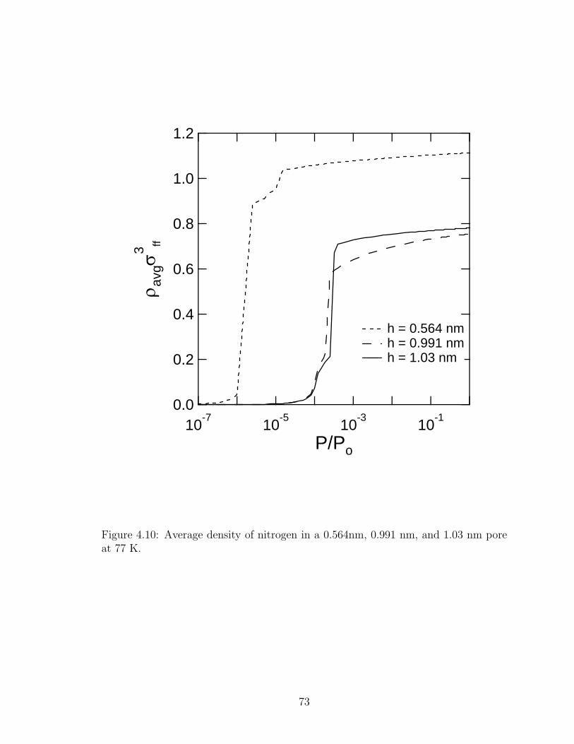
1.2

1.0

0.8

0.6

0.4

0.2

0.0

ρ avgσ3 ff

10-7 10-5 10-3 10-1 P/Po

h = 0.564 nm h = 0.991 nm h = 1.03 nm

Figure 4.10: Average density of nitrogen in a 0.564nm, 0.991 nm, and 1.03 nm poreat 77 K.

73

monolayer transition continues up to pores near 1 nm. For pores larger than 1 nm

the monolayer transition remains in the same place, but the pore condensation and

freezing transitions are moved to higher pressures.

Fig. 4.11 shows the PSD calculations for eq. 4.37 with three modes. Thirty

different pore isotherms like those shown in Fig. 4.10 were used in the calculations,

with 4 A pores used as the minimum size. The nitrogen isotherm used in the

calculations was from Russell and LeVan.83 There is a peak centered at 5.6 A with a

broad tail in larger pores. The PSD was also run with four modes but no substantial

differences were seen.

Fig. 4.12 is the calculated isotherm based on the calculated PSD with three

modes. The calculated isotherm describes the data well.

Pentane

For n-pentane the data from Avgul and Kiselev85 were used to estimate the

parameters, using the procedure described in Section . Results are given Table 4.1.

The parameters were fit using the pressure range from 0.01 up to 10 kPa. The carbon

used was a graphatized carbon black with a BET surface area of 12.2 m2/g. Again,

a pore with a half width of h = 20 σff was used to simulate a non-porous surface,

with results shown in Fig. 4.13.

Fig. 4.14 shows the density profiles, calculated using eq. 4.32, for a pore width

of 4.81 A. Fig. 4.14a shows the density profile of n-pentane at a pressure of 6.2×10−7

kPa; the system is well below the monolayer transition. Fig. 4.14b shows the den-

sity profile at a pressure of 1.16×10−4 kPa; at this pressure the system has gone

through condensation. Fig. 4.15 shows the density profiles for a pore of width 6.07

A. Fig. 4.15a is at a pressure of 6.2×10−7 kPa, which is well below the monolayer

transition. Fig. 4.15b is at a pressure of 3.5×10−3 kPa, and the fluid in the pore

has condensed. Fig. 4.16 shows the average density profiles, calculated with eq. 4.10,

74

30

25

20

15

10

5

0

f(h) (

cm3 / k

g Å

)

302520151050

h (Å)

Figure 4.11: Pore size distribution calculated from nitrogen density profiles with threemodes in eq. 4.37.

75

11

10

9

8

7

6

5

Load

ing

(mol

/kg)

4 6 8

10-42 4 6 8

10-32 4 6 8

10-2

Reduced Pressure (P/Po)

Figure 4.12: Nitrogen isotherm at 77 K on BPL activated carbon. Solid line is thecalculated isotherm.

76

1.4

1.2

1.0

0.8

0.6

0.4

0.2

0.0

Vol

ume

adso

rbed

(cc/

g (S

TP))

0.01 0.1 1 10

P (kPa)

Figure 4.13: Comparison of experimental and theoretical adsorbed volumes of pentaneon nonporous carbon black at 293.15 K. The points are experimental data. The solidline is the model predictions.

77

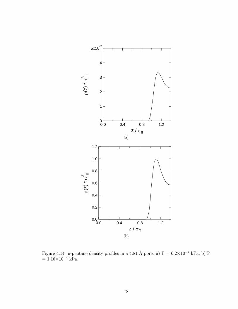
5x10-2

4

3

2

1

0

ρ(z)

* σ

3 ff

1.20.80.40.0z / σff

(a)

1.2

1.0

0.8

0.6

0.4

0.2

0.0

ρ(z)

* σ

3 ff

1.20.80.40.0z / σff

(b)

Figure 4.14: n-pentane density profiles in a 4.81 A pore. a) P = 6.2×10−7 kPa, b) P= 1.16×10−4 kPa.

78

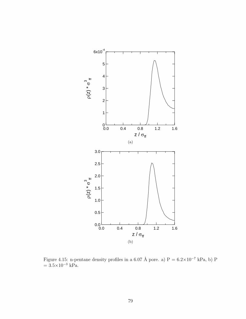
6x10-4

5

4

3

2

1

0

ρ(z)

* σ

3 ff

1.61.20.80.40.0z / σff

(a)

3.0

2.5

2.0

1.5

1.0

0.5

0.0

ρ(z)

* σ

3 ff

1.61.20.80.40.0z / σff

(b)

Figure 4.15: n-pentane density profiles in a 6.07 A pore. a) P = 6.2×10−7 kPa, b) P= 3.5×10−3 kPa.

79

for pores of size 4.81 A, 6.07 A, and 9.98 A. The position at which the condensation

steps ends in the pores of width 4.81 A and 6.07 A, with the isotherms flattening

out, are apparent. Also, it can be seen that fluid in the pore of width 9.98 A does

not go through condensation. This follows also for larger pores in the pressure range

examined.

The density profiles were calculated at 25 oC and compared with adsorption

data for n-pentane on BPL activated carbon from Schindler et al.86 Using the PSD

calculated with the nitrogen model an isotherm for n-pentane was determined by

combining the PSD, eq. 4.37, with the adsorption integral equation, eq. 4.36, using

forty calculated pore isotherms for pentane. The calculated isotherm is shown in

Fig. 4.17 as the solid curve. There is good agreement between the data and the model

predictions over a wide range of pressures. However, the data points of Schindler et

al.86 are not for pure n-pentane, but a binary mixture of n-pentane in nitrogen

carrier gas. If the ideal adsorbed solution theory is used to calculate the effect of

the nitrogen at the lowest loadings, it shows that the n-pentane partial pressure is

increased significantly. However, we believe that this is not entirely correct because

of a few reasons. Ideal adsorbed solution theory was developed for a homogeneous

surface. In the Henry’s law region, n-pentane is finding the high energy sites to

adsorb on in the heterogeneous BPL carbon, and these sites are not influenced much

by nitrogen. In the loading just above 0.01 mol kg−1, where the n-pentane is out of the

Henry’s law region, we may see the effects of the nitrogen. The n-pentane is adsorbing

on lower energy sites and is competing with the nitrogen causing the partial pressure

of n-pentane to increase slightly. A difference can be seen between the measured and

predicted values in this range. Also, as the loading approaches 1 mol kg−1 the effects

of the nitrogen are diminishing because the n-pentane is dominating in the system.

This is demonstrated by the convergence of the predicted and measured isotherms.

80

10-10

10-9

10-8

10-7

10-6

10-5

10-4

10-3

10-2

10-1

100ρ a

vgσ3 ff

10-10 10-8 10-6 10-4 10-2

P (kPa)

h = 4.81 Å h = 6.07 Å h = 9.98 Å

Figure 4.16: Average density of n-pentane in 4.81 A, 6.07 A, and 9.98 A pores at298.15 K.

81

10-5

10-4

10-3

10-2

10-1

100

101Lo

adin

g (m

ol/k

g)

10-10 10-8 10-6 10-4 10-2

Pressure (kPa)

Figure 4.17: Calculated n-pentane isotherm at 25oC on BPL activated carbon. Thecircles are the data from Schindler et al.86 The solid line is the isotherm based on thepore size distribution calculated by nitrogen.

82

4.4 Conclusions

A model was developed that adds the SAFT equation of state to DFT. This

was achieved by adding, for the first time, a first order attractive term where a mean-

field was not assumed, and by the addition of a second order attractive term. This

addition allows molecules to be treated as chain molecules, as opposed to just spher-

ical molecules. The model shows agreement with published Monte Carlo simulation

models for hard sphere chains of 3, 4, and 20 monomers near a hard wall. The model

was also compared with a 3-mer with a square-well attractive potential near both a

hard wall and an attractive wall.

The model was then used to determine the interaction parameters of nitrogen

and n-pentane with a carbon wall. The calculated density profiles show the presence

of the monolayer transition, pore condensation, and the freezing transition. When

the pore size places the larger peaks closer than 1 σ apart in the center of the pore,

apparent layering interactions are created. These turn into minor peaks surrounding

the major peak. The freezing transition has also been observed with the bases of the

peaks narrowing and the heights of the peaks increasing.

The PSD was calculated for BPL activated carbon using a log normal dis-

tribution with three modes and measured data for nitrogen at 77 K. The nitrogen

isotherm was described well using the pore size distribution.

Density profiles were then calculated for n-pentane. Pore condensation was

observed in the smallest pores. An isotherm for n-pentane at 25oC on BPL activated

carbon was calculated using the density profiles and the pore size distribution calcu-

lated from the nitrogen data. There is good agreement between the measured and

predicted isotherms. However, the data points are for a mixture of nitrogen and n-

pentane. This is believed to affect only the data in the mid range, out of the Henry’s

law region but before the n-pentane begins to dominate the adsorption space.

83

References

[1] G. J. Gloor, G. Jackson, F. J. Blas, E. M. Rio, and E. Miguel, J. Chem. Phys.

121, 12740 (2004).

[2] G. J. Gloor, F. J. Blas, E. M. Rio, E. Miguel, and G. Jackson, Fluid Phase Equil.

194-197, 521 (2002).

[3] P. Tarazona, Phys. Rev. A 31, 2672 (1985); 32, 3148 (1985).

[4] P. Tarazona, U. Marini Bettolo Marconi; and R. Evans, Mol. Phys. 60, 573

(1987).

[5] C. Lastoskie, K. E. Gubbins, and N. Quirke, J. Phys. Chem. 97, 4786 (1993).

[6] C. Lastoskie, K. E. Gubbins, and N. Quirke, Langmuir 9, 2693 (1993).

[7] R. J. Dombrowski, D. R. Hyduke, and C. M. Lastoskie, Langmuir 16, 5041

(2000).

[8] D. L. Valladares, F. R. Reinoso, and G. Zgrablich, Carbon 36, 1491 (1998).

[9] P. I. Ravikovitch, A. Vishnyakov, R. Russo, and A. V. Neimark, Langmuir 16,

2311 (2000).

[10] M. El-Merraoui, M. Aoshima, and K. Kaneko, Langmuir 16, 4300 (2000).

[11] P. I. Ravikovitch, A. Vishnyakov, and A. V. Neimark, Phys. Rev. E 64, 011602

(2001).

[12] M. B. Sweatman, and N. Quirke, Langmuir 17, 5011 (2001).

[13] S. K. Bhatia, Langmuir 18, 6845 (2002).

[14] T. Ohba, D. Nicholson, and K. Kaneko, Langmuir 19, 5700 (2003).

84

[15] Jagiello, J.; Thommes, M. Carbon 2004, 1227 .

[16] T. X. Nguyen, and S. K. Bhatia, Langmuir 20, 3532 (2004).

[17] E. A. Ustinov, and D. D. Do, Langmuir 20, 3791 (2004).

[18] P. I. Ravikovitch, S. C. O Domhnaill, A. V. Neimark, F. Schuth, and K. K.

Unger, Langmuir 11, 4765 (1005).

[19] E. A. Ustinov, and D. D. Do, J. Chem. Phys. 120, 9769 (2004).

[20] Y. Rosenfeld, Phys. Rev. Lett. 63, 980 (1989).

[21] Y. Rosenfeld, M. Schmidt, H. Lowen, and P. Tarazona, Phys. Rev. E 55, 4245

(1997).

[22] R. Roth, R. Evans, A. Lang, and G. Kahl, J. Phys: Condens. Matter 14, 12063

(2002).

[23] P. Bryk, R. Roth, K. R. Mecke, and S. Dietrich, Phys. Rev. E, 68, 031602 (2003).

[24] S. Figueroa-Gerstenmaier, F. J. Blas, J. B. Avalos, and L. F. Vega, J. Chem.

Phys., 118, 830 (2003).

[25] E. Kierlik, M. L. Rosinberg, Y. Fan, and P. A. Monson, J. Chem. Phys., 101,

10947 (1994).

[26] A. Malijevsky, J. Chem. Phys., 126, 134710 (2007).

[27] R. Evans,Fundamentals of Inhomogenous Fluids (Marcel Dekker, New Yoork,

1992).

[28] M. S. Wertheim, J. Stat. Phys. 35, 19 (1984).


85



[32] E. A. Muller, K. E. Gubbins, Ind. Eng. Chem. Res. 40, 2193 (2001).

[33] I. G. Economou, Ind. Eng. Chem. Res. 41, 953 (2002).

[34] A. Gil-Villegas, A. Galindo, P. J. Whitehead, S. J. Mills, G. Jackson, and A. N.

Burgess, J. Chem. Phys. 106, 4168 (1997).

[35] C. McCabe, and G. Jackson, PCCP Phys. Chem. Chem. Phys. 1, 2057 (1999).

[36] C. McCabe, A. Galindo, and M. N. Garcia-Lisbona, Ind. Eng. Chem. Res. 40,

3835 (2001).

[37] C. McCabe, and S. B. Kiselev, Fluid Ph. Equil. 219, 3 (2004).

[38] C. McCabe, and S. B. Kiselev, Ind. Eng. Chem. Res. 43, 2839 (2004).

[39] C. McCabe, A. Galindo, A. Gil-Villegas, and G. Jackson, Int. J. Thermophys.

19, 1511 (1998).

[40] C. McCabe, A. Gil-Villegas, and G. Jackson, J. Phys. Chem. B 102, 4183 (1998).

[41] A. Galindo, L. J. Florusse, and C. J. Peters, Fluid Ph. Equil. 160, 123 (1999).

[42] E. J. M. Filipe, E. de Azevedo, L. F. G. Martins, V. A. M. Soares, J. C. G.

Calado, C. McCabe, and G. Jackson, J. Phys. Chem. B 104, 1315 (2000).

[43] E. J. M. Filipe, L. F. G. Martins, J. C. G. Calado, C. McCabe, and G. Jackson,

J. Phys. Chem. B 104, 1322 (2000).

[44] L. M. B. Dias, E. J. M. Filipe, C. McCabe,and J. C. G. Calado, J. Phys. Chem.

B 108, 7377 (2004).

86

[45] L. X. Sun, H. G. Zhao, S. B. Kiselev, and C. McCabe, Fluid Ph. Equil. 228, 275

(2005).

[46] L. X. Sun, H. G. Zhao, S. B. Kiselev, and C. McCabe, J. Phys. Chem. B 109,

9047 (2005).

[47] H. Zhao, P. Morgado, C. McCabe, and A. Gil-Villegas, J. Phys. Chem. B 110,

24083 (2006).

[48] L. X. Sun, H. G. Zhao, and C. McCabe, AIChE J. 53, 720 (2007).

[49] C. McCabe, A. Galindo, A. Gil-Villegas, and G. Jackson, J. Phys. Chem. B 102,

8060 (1998).

[50] P. Morgado, C. McCabe, and E. J. M. Filipe, Fluid Ph. Equil. 228, 389 (2005).

[51] P. Morgado, H. Zhao, F. J. Blas, C. McCabe, L. P. N. Rebelo, and E. J. M.

Filipe, J. Phys. Chem. B 111, 2856 (2007).

[52] L. M. B. Dias, R. P. Bonifacio, E. J. M. Filipe, J. C. G. Calado, C. McCabe,

and G. Jackson, Fluid Ph. Equil. 205, 163 (2003).

[53] C. McCabe, A. Galinod, and P. T. Cummings,J. Chem. Phys. B 107, 12307

(2003).

[54] A. Valtz, A. Chapoy, C. Coquelet, P. Paricaud, and D. Richon, Fluid Ph. Equil.

226, 333 (2004).

[55] A. Galindo, A. Gil-Villegas, P. J. Whitehead, G. Jackson, and A. N. Burgess, J.

Phys. Chem. B 102, 7632 (1998).

[56] A. Galindo, and F. J. Blas, J. Phys. Chem. B 106, 4503 (2002).

[57] C. M. Colina, G. Galindo, F, J. Blas, and K. E. Gubbins, Fluid Ph. Equil. 222,

77 (2004).

87

[58] C. M. Colina, and K. E. Gubbins, J. Phys. Chem. B 109, 2899 (2005).

[59] D. Chandler, J. D. McCoy, and S. J. Singer, J. Chem. Phys. 85, 5971 (1986).

[60] D. Chandler, J. D. McCoy, and S. J. Singer, J. Chem. Phys. 85, 5977 (1986).

[61] J. D. McCoy, S. J. Singer, and D. Chandler, J. Chem. Phys. 87, 4853 (1987).

[62] J. Forsman, and C. E. Woodward, J. Chem. Phys. 119, 1889 (2003).

[63] A. Yethiraj, and C. E. Woodward, J. Chem. Phys. 102, 5499 (1995).

[64] Z. C. Ye, J. Cai, H. L. Liu, and Y. Hu, J. Chem. Phys. 123, 194902 (2005).

[65] Z. C. Ye, H. Y. Chen, H. L. Liu, Y. Hu, and J. W. Jiang, J. Chem. Phys. 126,

134903 (2007).

[66] S. Tripathi, and W. G. Chapman, J. Chem. Phys. 122, 094506 (2005).

[67] A. Dominik, S. Tripathi, and W. G. Chapman, Ind. Eng. Chem. Res. 45, 6785

(2006).

[68] S. Jain, A. Dominik, and W. G. Chapman, J. Chem. Phys. 127, 244904 (2007).

[69] Y. X. Yu, and J. Z. Wu, J. Chem. Phys. 116, 7094 (2002).

[70] Y. X. Yu, and J. Z. Wu, J. Chem. Phys. 117, 2368 (2002).

[71] Y. X. Yu, J. Z. Wu, Y. X. Xin, and G. H. Gao, J. Chem. Phys. 121, 1535 (2004).

[72] J. Chang, and S. I. Sandler, Molecular Physics 81, 735 (1994).

[73] L. Verlet, and J. J. Weis, Phys. Rev. A 5, 939 (1972).

[74] B. H. Patel, H. Docherty, S. Varga, A. Galindo, and G. C. Maitland, Molecular

Physics 103, 129 (2005).

88

[75] B. J. Zhang, Chem. Phys. Lett. 296, 266 (1998).

[76] B. J. Zhang, Fluid Phase Equil. 154, 1 (1999).

[77] B. J. Zhang, Fluid Phase Equil. 180, 182 (2001).

[78] Steele, W. A. Surf. Sci. 1973, 36, 317 .

[79] E. Kierlik, M. L. Rosinberg, J. Chem. Phys. 100, 1716 (1994).

[80] R. Dickman, C. K. Hall, J. Chem. Phys. 89, 3168 (1988).

[81] A. Yethiraj, C. E. Woodward, J. Chem. Phys. 102, 5499 (1995).

[82] M. Kruk, Z. Li, and M. Jaroniec, Langmuir 15, 1435 (1999).

[83] B. P. Russell, and M. D. LeVan, Carbon 32, 845 (1994).

[84] N. A. Seaton, J. P. R. B. Walton, and N. Quirke, Carbon 27, 853 (1989).

[85] N. N. Avgul, and A. V. Kiselev.(1970) In. Chemistry and Physics of Carbon. P.

Walker (Eds.) Vol. 6, M. Dekker, New York, pg 1-124.

[86] B. J. Schindler, L. C. Buettner, and M. D. LeVan, Carbon, 46, 1285 (2008).

89

CHAPTER V

CONCLUSIONS AND RECOMMENDATIONS

The research in this dissertation is centered around three main themes. The first is

the measurement of adsorption equilibrium data into the Henry’s law region. The

second area is the isosteric heat of adsorption calculated as a function of the pore

width in the Henry’s law region and determination of the pore width for which the

isosteric heat is a maximum. Finally, the third area is in the modification of density

functional theory to model chain fluids.

Chapter II

In this chapter, two new methods were used to prepare pre-equilibrated adsorption

samples at known loadings down to loadings of 0.0001 mol kg−1. The samples were an-

alyzed using a purge and trap method that allowed measurement into the Henry’s law

region. The adsorption data were compared with three known adsorption isotherms

and how well they fit the data as it transitions into the Henry’s law region. This

is the first time that adsorption was measured into the Henry’s law region for an

adsorbate that is a liquid at room temperature. The conclusions for this chapter can

be summarized as

• A new method for preparing samples at known loading from 1.0 down to 0.0001

mol kg−1 by liquid or gas injections was introduced.

• Isotherms for n-pentane on BPL activated carbon at temperatures from 0 to

175o were measured using a purge and trap method.

• The measured isotherms entered into the Henry’s law region.

• The transition into the Henry’s law region happened near a loading of 0.01 mol

kg−1 for all temperatures.

90

• The DR equation and the Langmuir equation were shown not to describe the

data well over its range.

• The Toth equation was shown to describe the data well over the range of pressure

and temperature.

• The isosteric heat of adsorption was shown to increase with decreased loading,

but levels off entering the Henry’s law region.

Chapter III

In this section the isosteric heat of adsorption was calculated as a function of pore

width in the Henry’s law region for parallel slit pores. The conclusions are

• The isosteric heat of adsorption was calculated as a function of the pore width.

• The theoretical maximum isosteric heat of adsorption is 15 - 50 % higher than

the values typically calculated from adsorption isotherms of materials with pore

size distributions.

• The pore size of the maximum isosteric heat of adsorption is a strong function

of the collision diameter and a weak function of the well depth potential. It

occurs in a pore size only slightly larger than the collision diameter.

• Carbon materials with parallel slit pores used for adsorptive storage will not be

suitable for hydrogen but could be acceptable for methane, if designed correctly.

Chapter IV

This section examined the modification of density functional theory to model chain

molecules in parallel slit pores. The statistical associating fluid theory equation of

state was included to achieve this. We conclude the following

91

• DFT was modified to include the ability to model chains with a first and second

order attractive potential.

• The model was used to estimate parameters for nitrogen and n-pentane adsorp-

tion in carbon parallel slit pores.

• The monolayer transition was observed as a function of pore width, along with

condensation and the freezing transition.

• To the best of our knowledge, the freezing transitions observed have the sharpest

density profiles that have been found for adsorption in a slit pore.

• The nitrogen model was used to calculate a pore size distribution for BPL

activated carbon.

• The calculated pore size distribution was used to calculated an isotherm for

n-pentane.

Recommended future work

There are many possibilities for this work to be extended in the future.

• The n-pentane isotherms can be measured with helium as a carrier gas, elimi-

nating the effect of nitrogen. The pure n-pentane data, along with the data in

this work can be used to explore how the ideal adsorbed solution theory works

when one component is in the Henry’s law region while the other is not.

• The experimental techniques developed for ultralow concentration adsorption

equilibrium of n-pentane on BPL activated carbon can also be used in the study

of other adsorbates and adsorbents and also for mixtures.

• The maximum value of the isosteric heat of adsorption can be calculated for

different pore geometries, such as cylindrical.

92

• Isotherms for different molecules can be calculated from density functional the-

ory at higher pressures and loadings than those in this work.

93

APPENDIX A

SAMPLE PREPARATION

A.1 Initial preparation work

The activated carbon was ground from a 6 × 16 mesh to a 40 × 50 mesh with

a mortar and pestle and sieved to separate. A large amount of activated carbon was

regenerated by placing it in an adsorption bed in an oven at 200 oC. Helium gas was

used as a carrier gas at a flow rate of 0.5 L/min for 8 hours. While the carbon was

regenerating, a number was scratched on the bottom of the glass vial for identification

purposes. The glass vial was then weighed empty and the weight was recorded. After

the activated carbon was regenerated, approximately 2 grams were placed in the vial

and weighed. The weight of the amount of carbon placed in the vial was calculated

and recorded. For samples of 0.01 mol kg−1 and above liquid injections were used.

For samples with loadings 0.01 mol kg−1 or lower gas injections were used.

After the samples were prepared by the methods described in the following two

sections, the ampules were leak checked by submersion in water. The samples were

then strapped to a ferris wheel arrangement in an environmental chamber, heated to

150 oC, and rotated end-over-end at 4 rpm for days to months to increase the mixing

of the solid and gas phases as equilibrium was established.

A.2 Liquid Injection

This section is for the preparation of samples with loadings of 0.01 mol kg−1

or greater. The glass ampule mentioned in the previous section, which contains 2

grams of regenerated carbon, was connected to the apparatus designed to prepare

samples by liquid injection, see Fig. 2.1a. The sample was then heated to 150o and a

vacuum was applied to the system for 8 hours, until the system reached a pressure of

94

0.05 mbar. The sample was removed from the heat, while maintaining a vacuum, and

placed in an ice bath. A syringe was used to inject a known amount of n-pentane into

the system. Before the syringe was used it was weighed and the system was removed

from the vacuum. After the syringe was used it was weighed again to determine the

weight of pentane injected into the system. The ampule was then sealed using a

micro-torch and the entire sample was weighed to calculate the mass of carbon used.

A.3 Gas Injection

This section is for the preparation of samples with loadings of 0.01 mol kg−1

or lower. Instead of injecting a liquid with a syringe, a system was designed to inject

a saturated vapor, thus allowing control of the amount injected into the system.

This system was designed because of the inability to control the amount injected

for amounts less then 1 µL. The system used a temperature bath to control the

temperature of a reservoir of pentane allowing us to control the concentration of the

vapor phase by use of saturated vapor. The saturated vapor was injected into the

system using a six-port valve and a sample loop. The temperature of the bath and the

size of the sample loop were determined by the sample size and the desired loading.

The ampule with the regenerated activated carbon was connected to the ap-

paratus shown in Fig. 2.1b. The sample was placed under vacuum and heated to

150oC for 8 hours, until the system reached a pressure of 0.05 mbar. The vacuum

downstream of the six-port valve was used to evacuate the system of any impurities.

Once the temperature bath was at the desired temperature and the measured pres-

sure was the vapor pressure of the pentane, the ampule was removed from the heat

and placed in an ice bath. The sample was removed from the vacuum and the valve

was switched exposing the system to the vapor in the sample loop. The ampule was

then sealed with a micro-torch and weighed to calculate the mass of activated carbon.

95

APPENDIX B

OPERATION PROCEDURE FOR THE DYNATHERM SYSTEM

The operating procedure for running the Dynatherm system through the Lab-

VIEW program was important for measuring accurate data into the Henry’s law

region. Before starting, the program PCswitch needs to be set to “GConly” and the

GC is on. The GC software program ChemStation is started. As the software is

booting up, it asks about addons, click yes. In the Run Control menu for ChemSta-

tion, click on Sample Info option. Give the samples a name. To name the samples

I used a format of MMDDYY#, where the # is the number of samples run that

day; I started with A. Do not forget to reset the counter number to 1, this is the

number of runs done on that sample; it will automatically increase after each run.

On the Dynatherm set the value for Dry, Heat, Cool, Trap, and Recyle. Set Dry to

zero minutes. The value of Heat was determined by experimentation to determine

the time step that fully regenerates the sample tube, but the sample does not break

through the focusing trap; it was set to four minutes. Set Cool to zero minutes. The

value of Trap was determined by them same method as the value of Heat; it was set

to four minutes. The value of Recycle determines the system recovery time if it is

desired to run the system without the labview program.

The following procedure is how to set and use the LabVIEW program that

controls the Dynatherm.

1. Open program LV7 0VaporPressure II mod3.vi

2. On front page

• Hit the run button

• GC Run time box

96

– Set the value to the length of the GC run. The value must be smaller

than the total run time set in the method file.

• Dynatherm Runtime box

– Sets the value the dynatherm runs. Is equal to the sum of external,

Dry, Heat, and Cool.

3. Go to the Configure menu

(a) Click on Sampling

• Make sure that the mode is set to continous

• In the operate menu, click Apply now

• In the file menu, click done

(b) Click on Experiments

• Check the operator name, change if necessary

• In the General section change to following if necessary

i. Chemical name

ii. Retention time

iii. Tol (+/-)

• In the Profiles section change

i. External Sample time. Set to the value that the dynatherm will

be collecting sample.

ii. Cylcle time. This is equal to the total of the dynatherm run time

(external+dry+heat+cool) plus the GC run time plus any time to

let the system cool down

iii. The temp, MFC settings are for the report only, does not change

anything

• Click on the Write File button.

97

– Name the file

– Use Dynatherm = yes

– Water bath present = no

– SCXI Present = no

4. In the operate menu click Run Now

5. When ready click start

To make permanent changes to the tables in the experiment section

1. Hit the stop button to stop the program

2. In the Browse menu go to the menu of This VI’s sub VI’s

• Click on the VI “WriteSetUp Plot II.vi”

– In the browse menu click on This VI’s sub VI’s

∗ Click on the VI “SetUpGlobal Plot II.vi”

∗ Make the changes in the tables as necessary

· To remove all entries from the table. Place cursor on the left

side of the table. Right click and chose data operations and click

on Empty Table

∗ In the operate menu click on make current values default

∗ In the file menu click on save

∗ Close the vi

– Close the vi

98

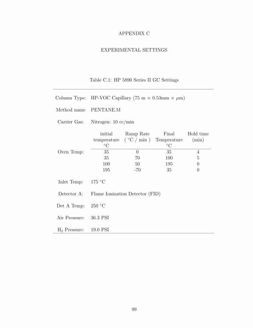
APPENDIX C

EXPERIMENTAL SETTINGS

Table C.1: HP 5890 Series II GC Settings

Column Type: HP-VOC Capillary (75 m × 0.53mm × µm)

Method name PENTANE.M

Carrier Gas: Nitrogen: 10 cc/min

Oven Temp:

initial Ramp Rate Final Hold timetemperature ( C / min ) Temperature (min)

C C35 0 35 435 70 100 5100 50 195 0195 -70 35 0

Inlet Temp: 175 C

Detector A: Flame Ionization Detector (FID)

Det A Temp: 250 C

Air Pressure: 36.3 PSI

H2 Pressure: 19.0 PSI

99

Table C.2: Dynatherm settings

Temperature Settings (C):

Valve Transfer line150 175

Tube TrapDesorb 310 350

Idle 25 25

Time Settings (min) :

Ext Dry— 0

Heat Cool4 0

Trap Recycle4 —

100

APPENDIX D

DENSITY FUNCTIONAL EQUATIONS

D.1 DFT

Density functional theory is based on a grand potential function

Ω[ρ(R)] = F +

∫ρ(R)[Vext(R)− µ]dR (D.1)

where ρM(R) is the density profile of a chain molecule and R ≡ (r1, r2, · · · , rM) is

the position vector. We are solving

δΩ[ρ(r)]

δρ(r)= 0 (D.2)

where ρ(r) is the segment density profile, and the Helmholtz free energy F is split up

into the ideal part

Fid[ρ(r)] = kT

∫ρ(r)

[ln(Λ3ρ(r))− 1

]dr (D.3)

and

δFid[ρ(r)]

δρ(r)= kT ln(Λ3ρ(r)) (D.4)

where Λ is the deBroglie wavelength, T is the temperature, and k is Boltzmann’s

constant. The hard sphere energy is

Fhs[ρ(r)] = kT

∫Φhs[ni(r)]dr (D.5)

and

δFhs[ρ(r)]

δρ(r)=

∫ ∑i

∂Φhs

∂ni(r)

∣∣∣∣r′

δni(r′)

δρ(r)dr′ (D.6)

where

Φhs(r) = Φhs1 + Φhs2 + Φhs3 (D.7)

Φhs1 = −n0 ln(1− n3) (D.8)

101

Φhs2 =n1n2 − nV 1 · nV 2

1− n3

(D.9)

Φhs3 =(n3

2 − 3n2nV 2 · nV 2)(n3 + (1− n3)2 ln(1− n3))

36πn23(1− n3)2

(D.10)

where

ni(r) =

∫ρ(r′)ωi(r− r′)dr′ (D.11)

i = 0, 1, 2, 3, V 1, V 2

ω3(r) = Θ(R− r) (D.12)

ω2(r) = |∇Θ(R− r)| = δ(R− r) (D.13)

ω1(r) =ω2(r)

4πR(D.14)

ω0(r) =ω2(r)

4πR2(D.15)

ωV 2(r) = ∇Θ(R− r) =r

rδ(R− r) (D.16)

ωV 1(r) =ωV 2(r)

4πR(D.17)

n3(z) = π

∫ z+R

z−R

ρ(z′)[R2 − (z′ − z)2]dz′ (D.18)

n2(z) = 2πR

∫ z+R

z−R

ρ(z′)dz′ (D.19)

nV 2(z) =

(−2π

∫ z+R

z−R

ρ(z′)(z′ − z)dz′)

z ≡ nV 2z (D.20)

∂Φhs

∂n0

= − ln(1− n3) (D.21)

∂Φhs

∂n1

=n2

1− n3

(D.22)

∂Φhs

∂n2

=n1

1− n3

+(n2

2 − nV 2 · nV 2)(n3 + (1− n3)2 ln(1− n3))

12πn23(1− n3)2

(D.23)

102

∂Φhs

∂n3

=n0

1− n3

+n1n2 − nV 1 · nV 2

(1− n3)2

+(n3

2 − 3n2nV 2 · nV 2)(n3 − 2(1− n3) ln(1− n3))

36πn23(1− n3)2

−(n32 − 3n2nV 2 · nV 2)(n3 + (1− n3)

2 ln(1− n3))

18πn33(1− n3)2

+(n3

2 − 3n2nV 2 · nV 2)(n3 + (1− n3)2 ln(1− n3))

18πn23(1− n3)3

(D.24)

∂Φhs

∂nV 1

= − nV 2

1− n3

(D.25)

∂Φhs

∂nV 2

= − nV 1

1− n3

− n2nV 2(n3 + (1− n3) ln(1− n3))

6πn23(1− n3)2

(D.26)

∫∂Φhs

∂n3

ω3(r− r′)dr′ = π

∫ z+R

z−R

∂Φ

∂n3

∣∣∣∣z′

[R2 − (z′ − z)2]dz′ (D.27)∫∂Φhs

∂n2

ω2(r− r′)dr′ = 2πR

∫ z+R

z−R

∂Φ

∂n2

∣∣∣∣z′dz′ (D.28)∫

∂Φhs

∂nV 2

ωV 2(r− r′)dr′ = 2π

∫ z+R

z−R

∂Φ

∂nV 2

∣∣∣∣z′

(z′ − z)dz′ (D.29)

the chain energy is

Fchain[ρ(r)] = kT

∫Φchain[nα(r)]dr (D.30)

and

δFchain[ρ(r)]

δρ(r)=

∫ ∑i

∂Φchain

∂ni(r)

∣∣∣∣r′

δni(r′)

δρ(r)dr′ (D.31)

where

Φchain(nα) =1−M

Mn0ζ ln yhs (D.32)

∂Φchain

∂n0

=1−M

Mζ ln yhs (D.33)

∂Φchain

∂n2

=1−M

Mn0

(∂ζ

∂n2

ln yhs + ζ

∂yhs

∂n2

yhs

)(D.34)

∂Φchain

∂nV 2

=1−M

Mn0

(∂ζ

∂nV 2

ln yhs + ζ

∂yhs

∂nV 2

yhs

)(D.35)

∂Φchain

∂n3

= n0ζ

∂yhs

∂n3

yhs

(D.36)

103

yhs =1

1− n3

+n2σζ

4(1− n3)2+

n22σ

2ζ

72(1− n3)3(D.37)

∂yhs

∂n2

=σ(ζ + n2

∂ζ∂n2

)

4(1− n3)2+σ2n2(2ζ + n2

∂ζ∂n2

)

72(1− n3)3(D.38)

∂yhs

∂nV 2

=

(σn2

4(1− n3)2+

σ2n22

72(1− n3)3

)∂ζ

∂nV 2

(D.39)

∂yhs

∂n3

=1

(1− n3)2+

σn2ζ

2(1− n3)3+

σ2n22ζ

24(1− n3)4(D.40)

and

ζ = 1− nV 2 · nV 2

n22

(D.41)

∂ζ

∂n2

=2nV 2 · nV 2

n32

(D.42)

∂ζ

∂nV 2

= −2nV 2

n22

(D.43)

The attractive potential is described by thermodynamic perturbation theory,

using first-order and second-order terms. The first-order term is described by

F1[ρ(r)] =1

2

∫ρ(r′)

∫ρ(r′′)ghs[n3(r

′′); r′′]φ(|r′ − r′′|)dr′′dr′ (D.44)

and the derivative is

δF1[ρ(r)]

δρ(r)=

∫ρ(r′)ghs[n3(r

′′); r′]φ(|r′ − r|)

+

∫ρ(r′)

∫ρ(r′′)

δghs[n3(r′′); r′′]

δρ(r′′)φ(|r′ − r′′|)dr′′dr′

(D.45)

where the attractive potential is a square-well potential

φ(r;λ) =

−εff if σ ≤ r < λσ0 if r ≥ λσ

(D.46)

and the hard sphere radial distribution function is calculated by

g(x) =1

x

∞∑n=0

U(x− n)Hn(x) (D.47)

where x = r/σ and U(x− n) is the unit step function. For the first shell 1 ≤ x < 2

H1(x) = a1 exp[A(x−1)]+a2 exp[B(x−1)] cos[C(x−1)]+a3 exp[B(x−1)] sin[C(x−1)]

(D.48)

104

where

A =−2η + zd

1− η(D.49)

B =−2η − zd/2

1− η(D.50)

C =

√3zs

2(1− η)(D.51)

zd = y+ − y− (D.52)

zs = y+ + y− (D.53)

y± = (2ηf)1/3

[(2η4

f 2+ 1

)1/2

± 1

]1/3

(D.54)

f = 3 + 3η − η2 (D.55)

η = (π/6)ρσ3 (D.56)

a1 =−2η(1− η − 3η2) + (1− 3η − 4η2)zd + (1 + η

2)z2

d

3(2η2 + z2d)(1− η)2

(D.57)

a2 =η(2 + 4η − 3η2)− (1− 3η − 4η2)zd + 2(1 + η

2)z2

d

3(2η2 + z2d)(1− η)2

(D.58)

a3 =(1− 3η − 4η2)(4η2 + z2

d) + η(2− 5η2)zd√3zs(2η2 + z2

d)(1− η)2(D.59)

for the second and third shells see the work of Chang and Sandler2

The second-order attractive term is described by

F2[ρ(r)] = − 1

4kT

∫ρ(r′)

∫ρ(r′′)(1 + 2ξn2

3)[φ(|r′ − r′′|)]2Khs(r′′)ghs[n3(r

′′); r′′]dr′dr′′

(D.60)

and the derivative is

δF2[ρ(r)]

δρ(r)= − 1

2kT

∫ρ(r′)(1 + 2ξn2

3)[φ(|r− r′|)]2Khs(r′)ghs[n3(r

′); r′]dr′

− 1

4kT

∫ρ(r′)

∫ρ(r′′)[φ(|r′ − r′′|)]2∂n3

∂ρ(4ξn3(r

′′)Khs(r′′)ghs[n3(r

′′); r′′]

+(1 + 2ξn3(r′′))

[∂Khs(r

′′)

∂n3(r′′)ghs[n3(r

′′); r′′] +Khs(r′′)∂ghs[n3(r

′′); r′′]

∂n3(r′′)

])dr′dr′′

(D.61)

where

ξ =1

η2con

(D.62)

105

where ηcon = 0.493 is the packing fraction where the fluid condenses.

Khs =(1− n3)

4

1 + 4n3 + 4n23 − 4n3

3 + n43

(D.63)

∂Khs

∂n3

=4(1− n3)

3(−2− 5n3 + n23)

(1 + 4n3 + 4n23 − 4n3

3 + n43)

2(D.64)

The external potential is described by

Vext = φsf (z) + φsf (H − z) (D.65)

where

φsf (z) = 2πεsfρsolσ2sf∆

[2

5

(σsf

z

)10

−(σsf

z

)4

−σ4

sf

3∆(z + 0.61∆)3

](D.66)

The expansion and rearrangement of eq. D.2 leads to the following equation

ρ(z) =1

Λ3exp(µ)

M∑i=1

exp [−βψ(z)]Gi(z)GM+1−i(z) (D.67)

where β = 1/kT , µ is the chemical potential described in the next section, and

ψ(z) =δFhs

δρ(r)+δFchain

δρ(r)+

δF1

δρ(r)+

δF2

δρ(r)+ Vext (D.68)

Gi =

∫exp[−βψ(z′)]

Θ(σ − |z − z′|)2σ

Gi−1dz′ (D.69)

where G1(z) = 1

D.2 Bulk Fluid

The chemical potential for the system is calculated by the following equations

for a bulk fluid. There are two different densities, the molecular density ρM and the

segment density ρs, where ρs = MρM . The chemical potential is calculated as the

derivative for the Helmholtz free energy with respect to ρM .

µ =∂A

∂ρM

(D.70)

106

For the ideal fluid the equations are

Aid,b = kTρM

[ln(Λ3ρM)− 1

](D.71)

µid,b = kT ln(Λ3ρM) (D.72)

For the hard sphere fluid the equations are

Ahs,b = kT

[−ρ0 ln(1− ρ3) +

ρ1ρ2

1− ρ3

+ρ3

2(ρ3 + (1− ρ3)2 ln(1− ρ3))

36πρ23(1− ρ3)2

](D.73)

µhs,b = MkT

[− ln(1− ρ3)

∂ρ0

∂ρs

+ρ2

1− ρ3

∂ρ1

∂ρs

+

(ρ1

1− ρ3

+ρ2

2(ρ3 + (1− ρ3)2 ln(1− ρ3))

12πρ23(1− ρ3)2

)∂ρ2

∂ρs

+

(ρ0(1− ρ3) + ρ1ρ2

(1− ρ3)2− ρ3

2 ln(1− ρ3)

18πρ33

− ρ32

36πρ23(1− ρ3)

− ρ32

36πρ23(1− ρ3)2

+ρ3

2

18πρ3(1− ρ3)3

)∂ρ3

∂ρs

](D.74)

where

ρ0 = ρs (D.75)

ρ1 = Rρs (D.76)

ρ2 = 4πR2ρs (D.77)

ρ3 =4

3πR3ρs (D.78)

For the chain term, the equation is

Achain,b = kT1−M

Mρ0 ln yhs,b (D.79)

µchain,b = kT (1−M)

(ln yhs,b

∂ρ0

∂ρs

+ ρ0

∂yhs,b

∂ρ2

y

∂ρ2

∂ρs

+ ρ0

∂yhs,b

∂ρ3

yhs,b

∂ρ3

∂ρs

)(D.80)

where

yhs,b =1

1− ρ3

+σρ2

4(1− ρ3)2+

σ2ρ2

72(1− ρ3)3(D.81)

The first order attractive potentials is described by

A1,b = −4ε(λ3 − 1)ηρsghs,e (D.82)

107

µ1,b = −4Mε(λ3 − 1)

(2ρ3ghs,e + ρ2

3

∂ghs,e

∂ρ3,e

∂ρ3,e

∂ρ3

)(D.83)

where

ghs,e =1− ρ3,e/2

(1− ρ3,e)3(D.84)

ρ3,e =C1n3 + C2ρ

23

(1 + C3ρ3)3(D.85)

∂ρ3,e

∂ρ3

=C1 + 2ρ3(C2 − C1C3)− ρ3C2C3

(1 + C3ρ3)4(D.86)

and C1

C2

C3

=

−3.16492 13.35007 −14.80567 5.7028643.00422 −191.66232 273.89683 −128.9333765.04194 −266.46273 361.04309 162.69963

1/λ1/λ2

1/λ3

1/λ4

(D.87)

The second-order attractive potential, derived by Zhang1 is given by

A2,b = −2βε2(λ3 − 1)[ρsρ3(1 + ξρ2

3)Khsghs,e

](D.88)

and the chemical potential is

µ2,b = −2Mβε2(λ3 − 1)

[4ξρ3

3Khsghs,e + (1 + 2ξρ23)

(2ρ3Khsghs,e + ρ2

3

[∂Khs

∂ρ3

ghs,e +Khs

∂ghs,e

∂ρ3,e

∂ρ3,e

∂ρ3

])](D.89)

D.3 Model Validation

The model has been tested against reference data as it was developed. For a

hard sphere system against a hard wall the model was tested against Monte Carlo

simulations done by Snook and Henderson.3 Fig. D.1 shows the model results for

reduced densities of ρσ3 = 0.57, 0.755, and 0.81, respectively. For hard sphere chains

against a hard wall and for systems with attraction, see Chapter IV.

108

2.4

2.2

2.0

1.8

1.6

1.4

1.2

1.0

0.8

0.6

0.4

0.2

ρ(z)

σ3

1.51.00.50.0

z/σ(a)

5.0

4.5

4.0

3.5

3.0

2.5

2.0

1.5

1.0

0.5

0.0

ρ(z)

σ3

1.51.00.50.0

z/σ(b)

7

6

5

4

3

2

1

0

ρ(z)

σ3

1.51.00.50.0

z/σ(c)

11

10

9

8

7

6

5

4

3

2

1

0

ρ(z)

σ3

1.51.00.50.0

z/σ(d)

Figure D.1: Hard spheres on hard wall. Monte Carlo simulations are by Snook andHenderson.3 The reduced densities are (a) 0.57, (b) 0.755, (c) 0.81, (d) 0.91. Thesolid curve is the model.

109

References

[1] Zhang BJ. Calculating thermodynamic properties from perturbation theory I.

An analytical representation of square-well potential hard-sphere perturbation

theory. Fluid Phase Equilibria 1999;154:1–10.

[2] Chang J, Sandler SI. A real function representation for the structure of the hard-

sphere fluid. Molecular Physics 1994;81:735–44.

[3] Snook IK, Henderson D. Monte Carlo study of a hard-sphere fluid near a hard

wall. J. Chem. Phys. 1978;68:2134–39.

110

APPENDIX E

ANALYSIS OF ALTERNATIVE NITROGEN ADSORPTION DATA BY

SAFT-DFT

Data of Joseph A. Rehrmann, personal communication, 1996. File AS650801.RAW

On the following pages is presented an analysis of an alternative data set for

nitrogen at 77 K on BPL activated carbon. Fig. E.1 shows the pore size distribution

calculated from the nitrogen istotherm data. Fig. E.2 shows the calculated and mea-

sured isotherm for nitrogen on BPL activated carbon. Fig. E.3 shows the calculated

pentane isotherm at 25 oC on BPL activated carbon using the calculated pore size

distribution.

111

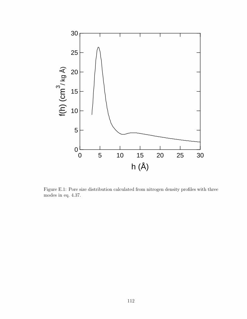
30

25

20

15

10

5

0

f(h) (

cm3 / k

g Å

)

302520151050

h (Å)

Figure E.1: Pore size distribution calculated from nitrogen density profiles with threemodes in eq. 4.37.

112

10

9

8

7

6

5

4

Load

ing

(mol

/kg)

10-52 4 6 8

10-42 4 6 8

10-32 4 6 8

10-2

Reduced Pressure (P/Po)

Figure E.2: Nitrogen isotherm at 77 K on BPL activated carbon. Solid line is thecalculated isotherm.

113

10-5

10-4

10-3

10-2

10-1

100

101Lo

adin

g (m

ol/k

g)

10-10 10-8 10-6 10-4 10-2

Pressure (kPa)

Figure E.3: Calculated n-pentane isotherm at 25oC on BPL activated carbon. Thecircles are the data from Schindler et al.1 The solid line is the isotherm based on thepore size distribution calculated by nitrogen.

114

References

[1] B. J. Schindler, L. C. Buettner, and M. D. LeVan, Carbon, 46, 1285 (2008).

115

henry’s law behavior and density functional theory analysis of adsorption...

Documents