Hedging and Pricing Options– using Machine Learning –

Jacob Michelsen Kolind, Jon Harrisand Karol Przybytkowski

December 10, 2009

Introduction

Options hedging has important applica-tions in risk management. In its most sim-ple form, options hedging is a trading strat-egy in a security and a risk-free bank ac-count. An option written on the securityis hedged by this strategy if the strategyis self-financing, and replicates the price ofthe option at all times and in all statesof the world. In the simple Black Scholesmodel, where only one source of uncer-tainty is present, it can be shown that suchstrategies do exist and an analytical ex-pression can be found for the proportion ofwealth that should be invested in the un-derlying security. For an options seller aswell as an options buyer, this trading strat-egy is important to know, since being shortthe option but long the hedging strategy orvice versa allows the seller/buyer to elimi-nate the risk associated with selling/buyingthe option.

In a real life setting, many of the Black-Scholes assumptions are violated. Thereare many sources of risk and agents in-cur transaction costs, so a perfect hedg-ing strategy cannot be expected to ex-ist. A more realistic approach for an op-tions trader is to minimize, not eliminate,their risk by rebalancing their portfolio dis-cretely. The size of the time steps be-tween adjustments would then depend onthe volatility of the market, the size of theportfolio, and the size of the transactioncosts incurred at each trading round. A

discretely rebalanced trading strategy willonly approximately hedge the option, andit is not immediately clear how to choosethe proportion of wealth to invest in theunderlying security at each trade. If weabstract away from choosing the size ofthe time steps between portfolio adjust-ments, we are left with an interesting ma-chine learning problem: How do we opti-mally choose the proportion of wealth toinvest in the security, the so called delta,∆, so that the value of our portfolio at thenext readjustment point in time is as closeas possible to the actual options price.

Data

We consider options data on theS&P500 index from the period 2009-01-02 09:30:01.052 to 2009-05-29 16:12:15.264.Our data set contains tick by tick data ofevery trade made in call and put optionson the index. Each observation containsthe following variables:

1. The time at which the trade tookplace, t.

2. The type of the option (call or put).3. The strike price of the option, K.4. The maturity date of the option, T .5. The S&P 500 index price, S.6. The price of the option, P .7. An implied volatility proxy, σ.

Since the numeraire in price data can be ar-bitrarily chosen, there is some redundancyin our data set. We choose to use the strike

1

Figure 1: Left panel: A 3D scatter plot of the call-options data including a fitted mesh.Right panel: A 3D scatter plot of the observed deltas including a fitted mesh.

price as the numeraire and thus henceforthonly look at ‘moneyness’, log(S/K), and‘calliness’/‘puttiness’, P/K. Ignoring thetime aspect of the data we have plotted (thedots)

P/K ∼ (log(S/K), (T − t))

in the left panel of Figure 1. Qualitativelythe data behaves very much as would be ex-pected from the Black Scholes model. Closeto maturity, P/K as a function of S/Kresembles a hockey stick, whereas furtheraway from maturity this hockey stick hasbeen smoothed out. The data contains ahigh degree of time variation. This can-not be seen from left panel of Figure 1, buta closer inspection of the data reveals thatthe surface has a positive thickness. If mar-ket conditions were stable arbitrage wouldforce the surface to have zero thickness.

By identifying options with the samestrike and maturity date, we extracted one-day movements in option prices and in-cluded that as an extra column in our data,(dP ). Corresponding to these one daymovements, we also extracted the move-ments in the S&P500 index, (dS). Ignoringinterest payments, the gain/loss of a strat-egy that buys one option and sells ∆ unitsof the index at time t and then reversesthese trades at time t+ 1 is

(P (t+ 1)−∆S(t+ 1))− (P (t)−∆S(t))= dP (t)−∆dS(t)

In the right panel of Figure 1 we have plot-ted dP/dS for those observations wheredS 6= 0. dP/dS corresponds to the valueof ∆ that would make the loss/gain of thehedging portfolio equal to zero.

Methodology

We explore two ways to model the priceand the optimal hedge: parametrically andnon-parametrically. The goal of both mod-els is first to be able to fit the surfaces likethe one displayed in Figure 1. For the pricesurface we use a weighted squared error lossfunction

P̂i 7→ wi(Pi − P̂i)2

where wi is a weight that will be specifiedshortly. For the delta surface we use theloss function

∆̂i 7→ wi(dPi − ∆̂dSi)2

= widS2i (dPi/dSi − ∆̂)2

i.e. a weighted version of the squaredloss/gain of the one-day hedge. Minimiz-ing both loss functions results in an WLSestimator of P̂ and ∆̂ respectively whenthese are considered as being functions ofthe covariates log-moneyness log(S/K) andtime to maturity T − t. Since neither sur-face looks like a hyperplane we approxi-mate them using fourth order tensor splineby a B-spline basis expansion of the stan-dard linear design matrix. Our parametric

2

Figure 2: Left panel: Seven days trailing realized volatility calculated from the spotS&P500 index price. Right panel: A plot of the cross-section at 0 < T − t < 50of the data plotted in the right panel of Figure 1. The blue points are fittedvalues.

model also includes a third covariate, trail-ing realized volatility, (σ̃), a measure of theobserved market volatility during the lastseven days before the data point. Trail-ing realized volatility, depicted in the leftpanel of Figure 2, is added to the para-metric model as a linear factor independentof the tensor spline basis in log(S/K) andT−t. Our calculations of realized volatilityfollows, to some extent, the papers by An-dersen et. al., 2003 and Barndorff-Nielsenet. al. 2002.

The trailing realized volatility is includedin the parametric model to accomodatethe time variation inherent in the data.That is, we use the trailing realized volatil-ity as a proxy for the time variation inthe data, and hope that the observed callprices/deltas can be described as noisyobservations of a function of the vector(log(S/K), T − t, σ̃). In the parametricmodel wi = 1.

Another way of incorporating time-variation into our model, the non-parametric approach, is to let the weights(wi) account for the time variation. Ourapproach is to let

wi = e−λ(t−ti)1{ti + δ > t > ti}

where ti is the time corresponding to ob-

servation i, and t is the time at which themodel is used for prediction. The non-parametric model weighs data points ob-served just prior to a point of predictionmore heavily than data points observed fur-ther away in the past1.

Results

Examples of how our models fit to the dataare displayed in the panels of Figure 1. Theplotted grids represent the fitted spline sur-faces.

It is most interesting to focus on the per-formance of our delta estimates. In theleft panel of Figure 3, a histogram of thedistribution of gains/losses using predicteddeltas for the month of April 2009 is dis-played. In the right panel, the correspond-ing distribution of gains/losses using BlackScholes deltas is displayed. The Black Sc-holes deltas are simply calculated using theformula

∆ = N

(log(S/K) + (r + σ2/2)(T − t)

σ√T − t

)where σ is the implied volatility and r is thethe risk-free interest rate. The Black Sc-holes delta should result in a perfect hedge

1δ is a fixed cutoff that sets weights that would otherwise have been very small to zero. This mitigatessome of the computational burden involved in fitting the non-parametric model.

3

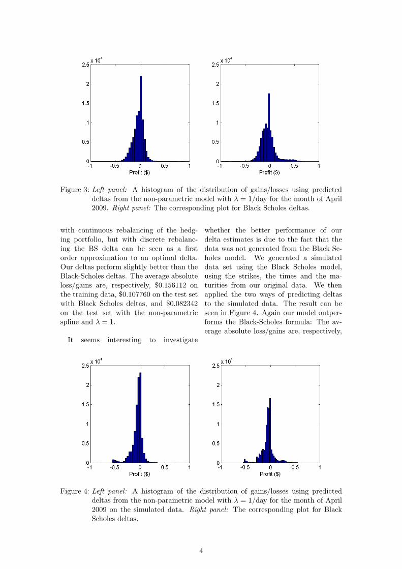
Figure 3: Left panel: A histogram of the distribution of gains/losses using predicteddeltas from the non-parametric model with λ = 1/day for the month of April2009. Right panel: The corresponding plot for Black Scholes deltas.

with continuous rebalancing of the hedg-ing portfolio, but with discrete rebalanc-ing the BS delta can be seen as a firstorder approximation to an optimal delta.Our deltas perform slightly better than theBlack-Scholes deltas. The average absoluteloss/gains are, respectively, $0.156112 onthe training data, $0.107760 on the test setwith Black Scholes deltas, and $0.082342on the test set with the non-parametricspline and λ = 1.

It seems interesting to investigate

whether the better performance of ourdelta estimates is due to the fact that thedata was not generated from the Black Sc-holes model. We generated a simulateddata set using the Black Scholes model,using the strikes, the times and the ma-turities from our original data. We thenapplied the two ways of predicting deltasto the simulated data. The result can beseen in Figure 4. Again our model outper-forms the Black-Scholes formula: The av-erage absolute loss/gains are, respectively,

Figure 4: Left panel: A histogram of the distribution of gains/losses using predicteddeltas from the non-parametric model with λ = 1/day for the month of April2009 on the simulated data. Right panel: The corresponding plot for BlackScholes deltas.

4

Figure 5: Left panel: Real data Right panel: Simulated data. The red dots are calculatedusing Black-Scholes deltas. Blue dots are spline fitted deltas.

$0.138111 on the training data, $0.096381on the test set with Black Scholes deltas,and $0.078296 on the test set with the non-parametric spline and λ = 1.

Figure 5 gives some intuition behind whyour method outperforms the Black-Scholesdelta. There is a convexity effect inher-ent in the Black Scholes deltas that cre-ates large gains when the underlying stockmoves a lot. Our method specifically tar-gets these large movements, using dS2 as aweight in the fitting, to try to minimize theimpact of these movements on the loss/gainin the hedging portfolio. The point cloudrepresenting gains/losses using our modelsthus curves less than the point cloud cor-responding to the analytical Black-Scholesdeltas. We are aware that some tradingstrategies exploit the convexity effect by

e.g. hedging straddles, but these kinds ofstrategies requires insight/an opinon aboutfuture volatility.

We do not present any results from theparametric model, since it, in its currentform, performed worse than the Black Sc-holes deltas.

Conclusion

We have presented a new way of estimatinggood delta hedges using tensor splines. Themethods we developed seem to work wellon simulated as well as real data, and gen-erally outperform the generic choice, theanalytical Black-Scholes delta hedging for-mula. Related to our work are the papersby Hutchinson et. al., 1994, Lai et. al.,2004 and Bennell et. al., 2005.

References

Andersen T. G., Bollerslev T., Diebold F. X. and Labys P., Modeling and Forecasting Realized Volatility,Econometrica, Vol. 71, No. 2 (Mar., 2003), pp. 579-625.

Barndorff-Nielsen O. E. and Shephard N., Econometric Analysis of Realized Volatility and Its Use inEstimating Stochastic Volatility Models, Journal of the Royal Statistical Society. Series B (StatisticalMethodology), Vol. 64, No. 2 (2002), pp. 253-280.

Bennell J. and Sutcliffe C., Black-Scholes versus artificial neural networks in pricing FTSE 100 options,Intelligent Systems in Accounting, Finance & Management, Vol. 12 Issue 4 2005 pp. 243-260.

Hutchinson J., Lo A. and Poggio T., A Nonparametric Approach to Pricing and Hedging DerivativeSecurities Via Learning Networks, Journal of Finance, Vol. 49 1994 pp. 851-889.

Lai T.L. and Wong S., Valuation of American options via basis functions, IEEE Transactions on Auto-

matic Control, Vol. 49 2004 pp. 374-385.

5