Pricing and Hedging Equity Indexed

Annuities with Variance-Gamma Deviates

Sebastian Jaimungal a

aDepartment of Statistics, University of Toronto,

100 St. George Street, Toronto, Ontario, Canada M5S 3G3

Version: 4 November 2004

Abstract

The author analyzes the pricing and hedging problem for Equity Indexed Annuities

(EIAs) with underlying risky assets following a geometric Variance-Gamma process.

This model allows accurate and parsimonious replication of the implied volatility

smiles observed in the financial market. I argue that this model produces consistency

in pricing and hedging between the financial and insurance markets. Closed form

expressions for prices of Point-to-Point and Cliquet instruments are developed and

used to investigate the break-even participation rates. Furthermore, I derive the

hedging parameters - Delta, Gamma and Vega - for the Cliquet design. Mortality risk

is incorporated through the Actuarial present value principal and I use numerical

experiments to investigate the effects of the model parameters.

Key words: , Equity Indexed Annuities, Guaranteed Investments, Jump Processes,

Variance Gamma Model

JEL codes: G13

Email address: sjaimung@utstat.utoronto.ca (Sebastian Jaimungal).1 The author thanks X.S. Lin and V.R. Young for useful discussions. This work was supported in

part by the Natural Science and Engineering Research Council of Canada.

2

1 Introduction

Equity-indexed annuities (EIAs) are considered to be one of the most innovative products in-

troduced into the insurance market in years. They have attained extremely high popularity in

recent times, reaching sales of over US $6 billion per annum. EIAs provide the annuitant with a

guaranteed return combined with the ability to earn a percentage of equity returns - borrowing

characteristics from both fixed-rate and variable-rate annuities. These insurance products have

recently come under intense focus; however, the analysis has been restricted to the case where

the underlying index price is modeled by a geometric Brownian motion (GBM). Tiong (2000)

successfully obtained closed form pricing formulae for various instruments, through Esscher

transformation methods, under the assumptions of GBM. Lin and Tan (2003) investigate the

effects of stochastic interest rates by postulating a Vasicek model for the short rate process

which is correlated to the GBM of the risky asset. They use simulation techniques to examine

the role that the various model parameters play. Their results demonstrate that stochastic

interest rates can affect the premiums and the break-even participation rates of the EIA prod-

ucts; however, for small to medium correlation coefficients the magnitude of these corrections

are fairly small, and the volatility of the index appears to be more important. This is to be

expected, because when the short rate and asset price process are uncorrelated, the interest

rate dynamics can be factored from the equity dynamics, and the pricing formulae which arise

are those of Tiong (2000) with r replaced by the average interest rate over the term of the

option, ravg = 1T−t

ln EQ[exp−

∫ Tt rs ds

]. In a market calibrated model, this average corre-

sponds to the prevailing spot interest rate of the appropriate maturity. Furthermore, although

EIA products typically have long terms (around 10 years) the embedded reset features are

typically applied over 12∼ 1 year periods. This implies that forward prices spanning a single

year or less are the most relevant, and such interest rates have significantly lower volatility

than, for example, a 10-year spot-rate.

In this paper, I extend the pricing formulae of Tiong (2000) to account for heavy tails and

3

skewness in the distribution of asset returns. The rationale being that most EIAs are writ-

ten on underlying indices for which there are heavily traded plain-vanilla put and call op-

tions. Furthermore, the market prices for such options are inconsistent with the assumption of

GBM, with the inconsistency reflected in the so called implied volatility smile and volatility

term structure, as well as in the statistical return distribution of asset prices. There are three

main classes of models which are capable of correctly matching market implied volatilities:

(i) state-dependent volatility models, (ii) stochastic volatility models, and (iii) jump models.

State-dependent volatility models attempt to capture the correlation between asset prices and

volatility. Non-parametric specifications have been investigated by Derman and Kani (1998)

and Duprie (1994); while parametric specifications have been invested by Cox and Ross (1976)

among many others. Stochastic volatility models assume that the volatility is driven by a sep-

arate stochastic process, which may be correlated to the asset price process. Hull and White

(1987) model the variance process as a diffusion process, while Duan (1996) utilizes a GARCH

model to model the two-dimensional dynamics. Jump models postulate that the asset price

follows a jump process, such as in the Poisson jump-diffusion model of Merton (1976), and in

the Variance-Gamma (VG) model introduced by Madan and Seneta (1990) and extended in

Madan, Carr, and Chang (1998).

I propose to use the geometric variance Gamma (VG) process to obtain EIA premiums which

are consistent with the market prices of puts and calls. The VG model is characterized by a time-

changed Brownian motion, where the time-change is driven by a Gamma process. Log-returns

of the underlying are assumed to be normally distributed in financial time rather than in real

time. The financial clock ticks in tandem with business activity; that is, during periods of high

activity the financial clock runs faster than the real clock, while during periods of low activity

the financial clock runs slower than the real clock. This model parsimoniously captures implied

volatility smile effects. Basic properties of the geometric VG process are reviewed in section 2

where I also introduce the main pricing results which are used throughout the remainder of

the paper.

4

In section 3, I obtain the premiums for EIAs with Point-to-Point and Cliquet designs and

explore how the model parameters affect this premium. In addition to consistently pricing the

EIA products, in section 4 I derive the dynamic hedging parameters Delta, Gamma, and Vega

implied by the VG model and illustrate how they differ from those implied by a GBM asset

model. I find that the differences can be dramatic and argue that heavy tails and skewness

must be taken into account to hedge EIAs properly. The financial risks in the EIA products

can be managed and priced through option theoretic methods; however, mortality risk must

also be accounted, and I achieve this through through standard Actuarial principles. In section

5 I show how the Actuarial present value principal can be used to price these products, and

also obtain the mortality adjusted hedging strategies.

2 The Variance-Gamma Model

The Variance-Gamma (VG) model has been chosen as a representative of the class of jump

models as it parsimoniously characterizes volatility smiles with three parameters: overall level

(σ), skewness (θ), and excess kurtosis (ν). Monroe (1978) demonstrated that any semimartin-

gale has a representation in terms of a time-changed Brownian motion. The VG model specifies

the time-change to be driven by a Gamma process. Monroe’s result implies that log-returns of

the underlying asset can be assumed to be normally distributed in financial time rather than

in calendar time. The ticking of the financial clock is correlated with business activity, so that

during periods of high activity the financial clock runs more quickly than the calendar clock,

while during periods of low activity the financial clock runs more slowly than the calendar

clock. The Gamma process is chosen to drive the financial clock for two reasons: (i) it is the

simplest continuous state-space analog of the Poisson process and (ii) it leads to a parsimo-

nious characterization of the two most important inherent biases in the Black-Scholes formula:

skewness and excess kurtosis.

Let Xt|t ≥ 0 denote a Brownian process with drift θ and volatility σ; further, let Γt|t ≥ 0

5

denote a Gamma process with variance rate ν and mean rate unity 2 . Let (Ω,F ,P) denote the

probability space with filtration F = Ft|t ≥ 0 where Ft, for every t ≥ 0, is the product sigma

field FXt ⊗FΓ

t , FX = FXt |t ≥ 0 is the natural filtration generated byXt, and FΓ = F Γ

t |t ≥ 0

is the natural filtration generated by Γt. The VG process is defined as a Brownian motion

subordinated by a Gamma process:

Yt ≡ XΓt . (1)

Remarkably, this process is in fact a pure jump Levy process and can be represented in terms of

its random jump measure µ(dy, dt), which counts the number of jumps arriving in the interval

[t, t+dt) of magnitude [y, y+dy) (see Bertoin, 1996; Sato, 1999). In terms of this jump measure

the VG process can be written as

Yt =

t∫0

∞∫−∞

y µ(dy, dt) . (2)

The predictable compensator of the jump process ν(dy) renders the compensated process Jt−

t∫∞−∞ ν(dy) a Martingale (see Bertoin, 1996; Sato, 1999). The compensator ν(dy) is known as

the Levy measure (or density), and is independent of t because of the stationarity of Levy

processes. For the VG model the Levy density can be written as

ν(dy) =1

ν|y|exp (by − a|y|) dy , (3)

where,

a =

2

νσ2+

(θ

σ2

)21/2

and b =θ

σ2. (4)

The characteristic function of Yt is supplied by the Levy-Khintchine formula

Φ(z) = EQ[eizXΓt

]= exp tψ(z) , (5)

2 A pure jump process and pure diffusion process contain orthogonal stochastic components as a

result of the Levy representation theorem, and are therefore immediately independent.

6

where,

ψ(z) =

∞∫−∞

(eizx − 1

)ν(dx) = −1

ν ln (1− i(a− b)z) + ln (1− i(a+ b)z) . (6)

From the above expression, the VG process can be viewed as the sum of two Gamma processes,

one with strictly positive and the other with strictly negative jump sizes. This proves the earlier

assertion that the VG process is indeed a pure jump model even though it is built as a time-

changed Brownian process.

The moments of the VG process can be computed from the cumulant ψ(x). The first four

moments are found to be:

E[XΓt ] = θ t , (7)

E[(XΓt − E[XΓt ])2] = (θ2ν + σ2) t , (8)

E[(XΓt − E[XΓt ])3] = (2θ2ν + 3σ2) ν θ t , (9)

E[(XΓt − E[XΓt ])4] = (3σ4 + 12σ2ν + 6θ4ν2) ν t+ (3σ4 + 6σ2θ2ν + 3θ4ν2) t2 . (10)

Notice that as θ tends to 0 the third moment vanishes; furthermore, the sign of θ determines

the sign of the skewness - positive skewness corresponds to positive θ, while negative skewness

corresponds to negative θ. Finally, in this limit, the fourth moment divided by the square of

the second is 3(1 + ν); consequently, ν characterizes the excess kurtosis in the model.

In this paper, the asset price process St is postulated to be a geometric VG process with a drift

adjustment directly under a given risk-neutral probability measure Q. Explicitly,

St = S0 exp ω t+XΓt . (11)

The asset is tradable only in real time, after the stochastic time change, and not in business

activity time (so that Γt is not an observable). The drift parameter ω is fixed by forcing the

dividend compensated asset price relative to the money-market account Mt = exp(∫ t0 rs ds) to

be a martingale, as follows:

7

EQ[eδtSt

Mt

∣∣∣∣∣Fs

]=eδsSs

Ms

⇒ ω = r − δ +1

νln(1−

(θ +

1

2σ2)ν). (12)

Here δ denotes the (constant) dividend yield rate of the asset and I assume that the short-rate

process is non-stochastic for simplicity. In particular rs is equal to r which is assumed to be

positive. The rate r is known as the force of interest by Actuaries.

The price of a European option written on a risky asset following a geometric VG process can be

obtained in three ways. Firstly, by utilizing Ito’s lemma for Levy processes to derive a partial-

integral-differential-equation (PIDE) that the price function solves; secondly, by utilizing the

characteristic function (5) to write the price in terms of the Fourier transformation of the pay-

off and the density; and thirdly, by utilizing the representation as a time changed Brownian

process. I find that the most useful representation for pricing EIAs is the third and the main

tool for determining their price is the following theorem.

Theorem 2.1 Given a European contingent claim which pays ϕ(ln(ST )) at time T , and assume

that the asset price process follows (11) under a given risk-neutral measure Q. The arbitrage-

free price at time t of such a claim, denoted Pt(s, T ) where s = ln(St), equals the time weighted

average of shifted Black-Scholes prices:

Pt(s, T ) =

∞∫0

exp(θ + 1

2σ2)g − rτ

PBS

(s+ ωτ, σ, θ +

σ2

2, g

)fΓτ (g) dg , (13)

where τ ≡ T − t, fΓτ (g) denotes the probability density function (pdf) of a Gamma random

variable,

fΓτ (g) =g

τν−1 e−

gν

Γ( τν) ν

τν, (14)

and the price of the option in the Black-Scholes model is,

PBS(s, σ, r, u) =e−ru

√2πσ2u

∞∫−∞

ϕ(s+ x) exp

−(x− (r − 1

2σ2)u

)2

2σ2u

dx . (15)

8

Madan, Carr, and Chang (1998) use a version of the above theorem to demonstrate that puts

and calls can be written in terms of degenerate Hypergeometric functions and Bessel functions.

The pricing formula they obtain are similar to the Black-Scholes case with the density function

for the standard normal replaced by the special function

Ψ(a, b, c) ≡∞∫0

Φ

(a√g

+ b√g

)gc−1e−g

Γ(c)dg , (16)

where Φ(x) denotes the cumulative density function (cdf) of a standard normal random vari-

able. The Ψ function is a weighted average of the normal cdf which arises in Black-Scholes

pricing equations - Ψ accounts for the effects of the stochastic time change. In the appendix,

the Ψ function is written in terms of Hypergeometric and Bessel functions. The price of Euro-

pean call and put options can be reduced to combinations of the Ψ function using proposition

2.1 resulting in the following pricing equation.

Theorem 2.2 Call Price Function. The value at time t < T of a call option with strike K

and maturity T written on an asset following a geometric VG process (11) is

Ct(T,K) = St e−δ τΨ

ς√ϑ

ν,θ + σ2

σ

√ν

ϑ,τ

ν

−K e−r τ Ψ

(ς√ν,θ

σ

√ν,τ

ν

), (17)

where,

ς =ln(St/K) + ωτ

σ, (18)

ϑ= 1− (θ + 12σ2) ν , (19)

and τ ≡ T − t.

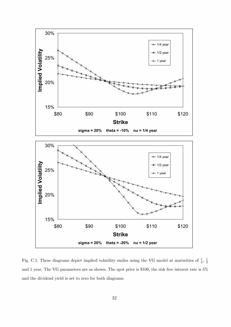
The VG model is able to capture a variety of features in the implied volatility smiles. Recall

that implied volatility σimp is the volatility in the Black-Scholes model which matches quoted

prices and is defined as the solution to the non-linear equation

CallBS(S,K, σimp, τ) = Call(S,K, τ) , (20)

9

where Call(S,K, τ) denotes the quoted price. Figure C.1 depicts several implied volatility smiles

at maturities of 14, 1

2and 1 year using the VG model prices as a proxy for market prices. The

risk-free rate has little effect on the general shape of the curves and is fixed at 5% per annum

for all maturities. Notice that the smiles are negatively skewed and steep in the shorter term,

while they flatten and become more symmetric in the long term. Such behavior is typically

observed in the financial markets across all sectors. The VG kurtosis parameter ν controls

the steepness while θ controls the asymmetry of the smiles. Negative θ is typically observed

in options on index futures as well as individual stock options. This implies that the market

values out-of-the money puts more highly than similar out-of-the-money calls.

3 Pricing Formulae

3.1 The Point-To-Point Design

A Point-to-Point EIA supplies the annuitant with a guaranteed minimum (continuously com-

pounded) return of γ on a percentage β of the notional amount from the time of entering the

contract to maturity T . The equity-linked return, which the minimum is compared with, is

scaled by the participation rate which I denote by α. The value of this contract at expiry is

written as follows:

ϕ(S0, ST ) = max

(β eγ(T−t),

(ST

S0

)α). (21)

The value of the contract at an arbitrary time t, such that 0 ≤ t ≤ T , is obtained by condi-

tioning on the Gamma time change and using (16). I record the pricing result in the following

theorem and delegate the proof to the appendix (in the remainder of this paper, all proofs are

deferred to the appendix).

Theorem 3.1 The value at time t, such that 0 ≤ t ≤ T , of a Point-to-Point EIA contract

10

written on an asset following a geometric VG process (11), is

P ppt (S0, St, α, β, γ, T )

= β e−r τ + γ T Ψ

(ς√ν,− θ

σ

√ν,τ

ν

)+(St

S0

)α e−(r−αω) τ

ϑτ/νΨ

−ς√ϑ

ν,θ

σ

√ν

ϑ,τ

ν

, (22)

where τ ≡ T − t represents the time to maturity,

ς =γ T − α(ω τ + ln(St/S0)) + ln(β)

ασ, (23)

θ= θ + ασ2 , (24)

and

ϑ= 1− α ν(θ +

1

2ασ2

). (25)

Figure C.2 shows the dependence of the initial premium of a Point-To-Point EIA as a function

of the time to maturity and the excess kurtosis parameter ν. For α less than one the behavior

of the premium is predominantly determined by the time to maturity while the excess kurtosis

has little affect. This is reassuring, since most products are being sold with participation

rates considerably less than unity, while most risk management systems are built around the

assumptions of Black-Scholes. However, when α is greater than one, the premiums are very

sensitive to the excess kurtosis parameter ν, and it becomes important to account for departures

from Black-Scholes.

The break-even participation rate, defined as the participation rate which makes the premium

of the contract exactly one, provides a benchmark for setting α. Tiong (2000) finds that the

theoretical Black-Scholes break-even points are considerably higher than those currently being

offered in the market. In Table C.1 the break-even participation rates for the Point-to-Point in-

strument under several market conditions are shown. In this table, the VG volatility parameter

σ is chosen such that the at-the-money implied volatility of a call option is equal to either 20%

or 30%. This allows for meaningful comparisons across different terms and interest rate levels.

11

On comparing Table C.1 with the results in Tiong (2000) one see that VG model implies lower

break-even participation rates than those implied by GBM. This agrees with intuition, since

accounting for jump risk induces an increase in the price of the contract for the same level of

participation; consequently, a lower participation is required to break-even. Even though the

VG-model implies lower participation rates, they are not sufficiently low to fully account for

current market practices.

3.2 The Cliquet Design

The Cliquet (or ratchet) design EIA provides several guarantees over the lifetime of the product.

At the end of each time period of length ∆t this EIA locks in a percentage α of the return on

the index; however, if the scaled return is lower the guaranteed minimum return of γ, then the

investor receives a return of γ for that period. The pay-off from this investment scheme is paid

at the maturity date, and can be expressed as,

ϕ(S0, S∆t, . . . , Sn∆t) =n∏

i=1

max

(eγ ∆t,

(Si∆t

S(i−1)∆t

)α). (26)

The value of such a contract at t less than ∆t is therefore

P ct (S0, St, γ, α,∆t, n) (27)

= EQ[e−r (n∆t−t)

n∏i=1

max

(eγ ∆t,

(Si∆t

S(i−1)∆t

)α)∣∣∣∣∣Ft

]

= EQ[e−r (n∆t−t) max

(eγ ∆t,

(S∆t

S0

)α)

n∏i=2

max

(eγ ∆t,

(Si∆t

S(i−1)∆t

)α)∣∣∣∣∣Ft

]

= e−r (∆t−t)EQ[max

(eγ ∆t,

(S∆t

S0

)α)∣∣∣∣∣Ft

]

×n∏

i=2

e−r ∆tEQ[max

(eγ ∆t,

(Si∆t

S(i−1)∆t

)α)∣∣∣∣∣F(i−1)∆t

]

=P ppt (S0, St, α, 1, γ,∆t) (P pp

0 (1, 1, α, 1, γ,∆t))n−1 . (28)

12

The third equality follows from the independent and stationary increment properties of the

Brownian motion and the subordinating Gamma process which generate the VG dynamics.

Notice that the premium, at t = 0, with n resets is equal to the premium of a one period EIA

raised to the power of n. The break-even points for these instruments are therefore equal to

those in a Point-to-Point design with a term of ∆t and a β of 100%. If the underlying process

is not stationary, then the pricing problem would be much less tractable. This is one major

advantage of the VG model - it is able to capture heavy tails and skewness while maintaining

analytical tractability.

3.3 The Cliquet with a Cap Design

The Cliquet design is also offered with a cap κ. The cap feature reduces the price of the guar-

antee, and therefore admits a higher break-even participation rate than the same instrument

without a cap. The embedded protection provided by the floor, along with the higher partic-

ipation rate, makes this product much more attractive than the Cliquet without a cap. The

pay-off at maturity is

ϕ(S0, S∆t, . . . , Sn∆t) =n∏

i=1

min

(eκ ∆t, max

(eγ ∆t,

(Si∆t

S(i−1)∆t

)α)). (29)

In the limit as κ tends to ∞ the capped Cliquet design reduces to the Cliquet design without a

cap. The general pricing problem can be treated by conditioning on the stochastic time change

and integrating over the remaining Brownian degree of freedom.

Theorem 3.2 The value at time t, such that 0 ≤ t < ∆t, of a capped Cliquet with n remaining

protection periods, written on an asset following a geometric VG process (11) is

P cct (S0, St, γ, α, κ,∆t, n) = P cc

t (S0, St, γ, α, κ,∆t) (P cc0 (1, 1, γ, α, κ,∆t))n−1 , (30)

where,

13

P cct (S0, St, γ, α, κ,∆t)

= e−rτ

eκ∆tΨ

(−ς(κ)√

ν,θ

σ

√ν,τ

ν

)+ eγ∆tΨ

(ς(γ)√ν,− θ

σ

√ν,

∆t

ν

)

+(St

S0

)α eαωτ

ϑτ/ν

[Ψ

ς(κ)√ϑ

ν,− θ

σ

√ν

ϑ,τ

ν

−Ψ

ς(γ)√ϑ

ν,− θ

σ

√ν

ϑ,τ

ν

] , (31)

and

ς(x) =1

σ

x∆t

α− (ωτ + ln(St/S0))

. (32)

Figure C.3 illustrates how the premium varies as a function of the participation rate and excess

kurtosis. As in the Point-to-Point case, the Black-Scholes premium forms a lower boundary for

the premiums at all levels of participation. The heavy tails and negative skewness place a

higher burden on the embedded guarantee resulting in higher premiums than the case without

such heavy tails or negative skewness. The general trend found in the GBM case is maintained;

however, the values themselves and curvatures are clearly larger in the VG model. Table C.2

contains the break-even participation rates for several model and contract parameters. The

excess kurtosis in the VG model induces at least a 10% reduction in the break-even participation

rates compared with the results reported in Tiong (2000).

4 Dynamic Hedging

In this section, I obtained the Delta, Gamma and Vega of a capped Cliquet (referred to as

a Cliquet in the sequel). These parameters can be used to dynamically hedge the market

risk component of the EIAs. Within an incomplete market model, such as the VG model,

dynamic hedging cannot be used to eliminate all risks; however, it will offer the risk manager

the ability to partially hedge them. The hedging parameters developed in this section will

certainly outperform those implied by the Black-Scholes model, as heavy tails and skewness

are explicitly incorporated into the pricing problem.

14

The Delta ∆t(St) of an option is defined as the relative change of the price of the option with

respect to small changes in the spot price. Let Pt(St) denote the price of an option with a spot

of St, then

∆t(St) ≡∂

∂St

Pt(St) . (33)

The Delta prescribes the number of units in the underlying asset that the risk manager can

hold to offset changes in the option price due to changes in the spot price. However, it is

well known that due to the curvature of option prices, as a function of the spot-level, Delta

hedging is insufficient for risk management purposes. This is especially true for options in

which the convexity changes sign, such as those embedded in EIA products. To properly hedge

such risks the options Gamma Γt(St) must be utilized, and offsetting positions in put and call

options must be used in conjunction with positions in the underlying asset to properly hedge

the position. The Gamma is defined as the sensitivity of the Delta as the spot changes and is

explicitly given by:

Γt(St) ≡∂

∂St

∆t(St) =∂2

∂S2t

Pt(St) . (34)

Finally, although spot price changes constitute the largest affect on the hedging strategy, the

market volatility may also change through time. To manage such risks the options Vega Vt(St),

measured by the sensitivity of price to volatility level, is used. Explicitly,

Vt(St) ≡∂

∂σPt(St) . (35)

In the VG-model, the parameter σ is not an absolute measure of the volatility level (it also

affects kurtosis and skewness, see equations (7-10)); however, it predominantly sets the vertical

position of the implied volatility smiles. Consequently, it is a reasonable proxy for the constant

volatility parameter in the Black-Scholes model and I propose that it be used to hedge against

changes in volatility level.

15

I now record the main results of this section, while delegating the proofs to the appendix.

Theorem 4.1 The Delta of the capped Cliquet EIA is,

∆cct (S0, St, γ, α, κ,∆t, n) = ∆cc

t (S0, St, γ, α, κ,∆t) (P cc0 (1, 1, γ, α, κ,∆t))n−1 (36)

where,

∆cct (S0, St, γ, α, κ,∆t)

=α

ϑτ/ν

Sα−1t

Sα0

e−(r−αω)τ

Ψς(κ)

√ϑ

ν, − θ

σ

√ν

ϑ,τ

ν

−Ψ

ς(γ)√ϑ

ν, − θ

σ

√ν

ϑ,τ

ν

. (37)

Theorem 4.2 The Gamma of the capped Cliquet EIA is,

Γcct (S0, St, γ, α, κ,∆t, n) = Γcc

t (S0, St, γ, α, κ,∆t) (P cc0 (1, 1, γ, α, κ,∆t))n−1 (38)

where,

Γcct (S0, St, γ, α, κ,∆t)

=α− 1

St

∆cct (st, γ, α, κ,∆t)

+2α e−rτ

σ S2t ν

τν Γ( τ

ν)

(ς2(γ)

a

) τ2ν− 1

4

eθ ς(γ)/σ+γ T K τν− 1

2

(2√a ς2(γ)

)

−(ς2(κ)

a

) τ2ν− 1

4

eθ ς(κ)/σ+κ T K τν− 1

2

(2√a ς2(κ)

) , (39)

and,

a=1

ν− 1

2

θ2

σ2. (40)

Furthermore, Kv(x) denotes the modified Bessel function of the second kind of order v.

Theorem 4.3 The Vega of the capped Cliquet EIA is,

Vcct (S0, St, γ, α, κ,∆t, n)

= Vcct (S0, St, γ, α, κ,∆t) (P cc

0 (1, 1, γ, α, κ,∆t))n−1

+(n− 1)P cct (S0, St, γ, α, κ,∆t)Vcc

0 (1, 1, S0, γ, α, κ,∆t) (P cc0 (1, 1, γ, α, κ,∆t))n−2 , (41)

16

where,

Vcct (S0, St, γ, α, κ,∆t)

= α(St

S0

)α

e(ωα−r)τ

ασν

ϑτν+1

Ψ

ς(κ)√ϑ

ν,− θ

σ

√ν

ϑ,τ

ν+ 1

−Ψ

ς(γ)√ϑ

ν,− θ

σ

√ν

ϑ,τ

ν+ 1

− τσ

(1− (θ + 12σ2)ν)ϑ

τν

Ψς(κ)

√ϑ

ν,− θ

σ

√ν

ϑ,τ

ν

−Ψ

ς(γ)√ϑ

ν,− θ

σ

√ν

ϑ,τ

ν

− 1

Γ( τν)ντ/ν

√2

π

eς(κ)θ

ς2(κ)

2ϑν

+ θ2

σ2

τ2ν

+ 14

K τν+ 1

2

√√√√√ς2(κ)

2ϑ

ν+θ

2

σ2

−eς(γ)θ

ς2(γ)

2ϑν

+ θ2

σ2

τ2ν

+ 14

K τν+ 1

2

√√√√√ς2(γ)

2ϑ

ν+θ

2

σ2

. (42)

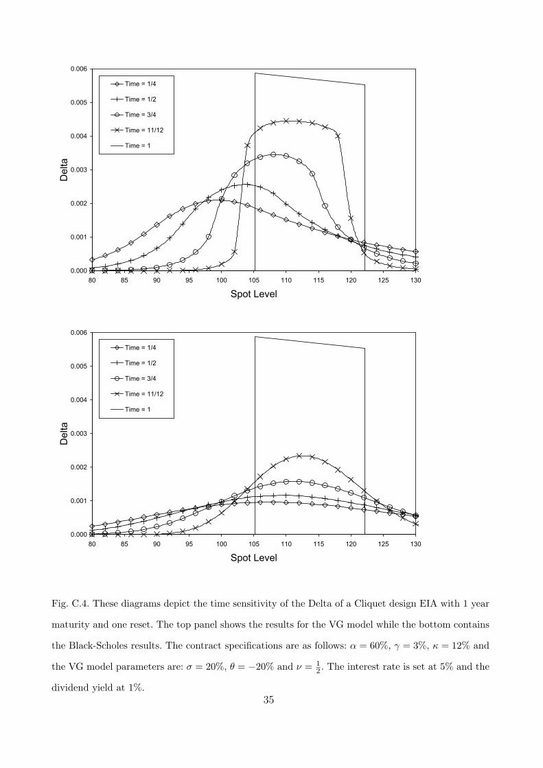
Figure C.4 depicts how the Delta, as a function of the spot price, evolves through time. The

top panel depicts the results in the VG-model and for comparison the Black-Scholes model

results are displayed in the lower panel. Notice that the Delta approaches its asymptotic value,

at the maturity date, much more quickly in the VG model than it does in the Black-Scholes

model.

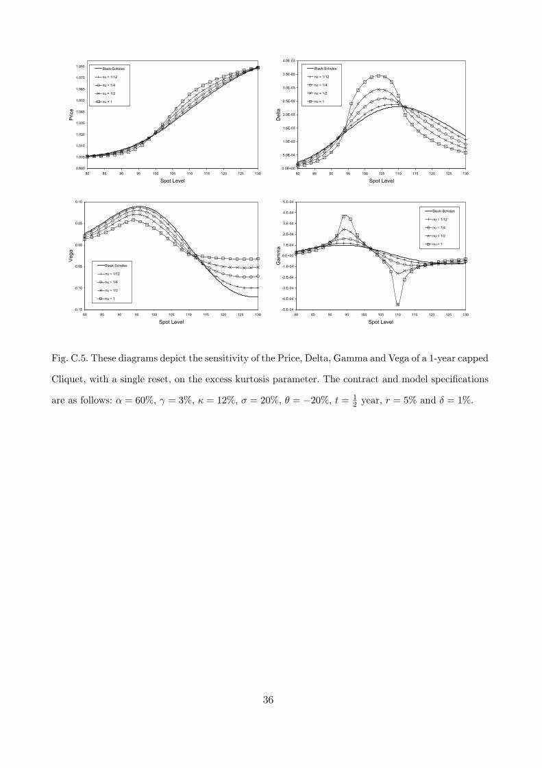
Figure C.5 depicts the behavior of the Price, Delta, Gamma and Vega, as a function of the

spot price, on the excess kurtosis parameter ν. In the in-the-money region the price increases

as ν increases, this results from an increase in the probability that the process jumps deeper

into the money. In the out-of-the-money region the price decreases as ν increases, this results

from an increase in the probability that the process jumps deeper out of the money.

The Delta also has an interesting behavior. As ν increases, the Delta increases in the region

in which the EIA pays the equity return, while it decreases outside this region. Thia is to say,

the Delta tends towards its value at maturity as ν increases. Unlike the Black-Scholes Delta,

which is essentially symmetric, the VG Delta is highly asymmetric due to the asymmetry in

17

the jump sizes.

The behavior of the Gamma is also consistent with the previous observations. As ν increases

the Gamma becomes more highly peaked near the spot prices where the floor and the cap

become effective. Also notice that the sign of Gamma changes from positive to negative.

Finally, the absolute size of the Vega of the EIA is smaller than the Black-Scholes case, in-

dicating that the option prices are less sensitive to changes in volatility level. This is to be

expected since the presence of tail events has a larger effect on price than small changes in the

volatility level.

5 Incorporating Mortality Risk

EIA contracts typically contain mortality clauses such as the following: if the annuitant dies

in year m, then the guaranteed return up to the end of that year is paid to the investors

beneficiary. If the insurance company is well diversified, in that the number of policies, with

the same contract parameters, are sold to a large number of individuals, then mortality risk

can be priced into the contracts rather simply using the Actuarial present value principle (see

Bowers, Gerber, Hickman, Jones, and Nesbitt, 1997). This assumes that the future lifetime T (x)

of the individual (x) is stochastically independent of the asset price process, and is certainly

a just assumption. Let tpx ≡ P(T (x) > t) denote the probability that an individual (x) will

survive past age t given that the individual is aged x. As usual the mortality probability is

defined as tqx = 1− tpx. The one year survival and mortality probability are defined as px ≡ 1px

and qx ≡ 1qx respectively. Assume that if the annuitant dies during the time interval [k, k+1),

then the annuity closes at the end of the year k + 1. The mortality modified pay-off for the

EIA contract, accumulated to the maturity date T = n∆t, is therefore

ϕ (S0, S∆t, . . . , Sn∆t, T (x))

= er (n−1)∆tϕ (S0, S∆t) I (T (x) ∈ (t,∆t])

18

+n∑

k=2

er (n−k)∆t ϕ (S0, S∆t, . . . , Sk∆t) I (T (x) ∈ ((k − 1)∆t, k∆t]) , (43)

where I(A) represents the indicator function for the event A and ϕ (S0, S∆t, . . . , Sk∆t) rep-

resents the pay-off of a k∆t-maturity EIA without mortality risk.

The Actuarial fair value of the contract is

Pt = EQ[ϕ (S0, S∆t, . . . , Sn∆t, T (x)) |F t] = Pt(N) Npx +N∑

k=1

Pt(k) k−1px qx+k−1 , (44)

where Pt(k) denotes the price, at time t, of the k-maturity EIA without mortality risk and

F t represents the product filtration generated by the asset and the time of death stochastic

processes. The break-even participation rate in a well diversified portfolio therefore solves

P0 = P (N)0 Npx +N−1∑k=0

P (k)0 kpx qx+k = 1 . (45)

If the portfolio is not well diversified, in that the number of issued annuities is small, one can

instead use a loaded participation rate, defined as the participation rate which solves

EQ[ϕ|F0] + ε√

VarQ[EQ[ϕ|T (x)]|F0] = 1 . (46)

A participation rate satisfying (46) will guarantee that ε% of the time there are sufficient funds

to cover the EIA benefits. Clearly this results in an equal or lower participation rate than that

computed by (45). The variance appearing in (46) is easily computed in terms of the prices of

the EIA product without mortality risk as follows:

VarQ[EQ[ϕ|T (x)]|F0] = P 20 (N) Npx +

N−1∑k=0

P 20 (k) kpx qx+k − P 2

0 . (47)

Interestingly, in an asset model which has stationary and independent increments, the break-

even participation rates with and without mortality risk are identical; furthermore, the loaded

break-even participation rate is equal to the unloaded rate. This is because in the case without

mortality there exists a single participation α, across all maturity levels, that sets the pre-

19

mium equal to one. This results from the power law behavior in for example equation (30).

Consequently, if such a rate is used in the presence of mortality risk, then summing over all

mortality events, weighted by their respective probabilities, also results in a premium of one.

Furthermore, since the premiums for all maturities are equal, the variance of the premiums is

identically zero and the loaded participation rate calculation reduces to the unloaded case.

Even though the break-even participation rates are unaffected by mortality risk in a stationary

model, the hedging parameters are are affected when mortality is present. In the presence of

mortality risk one finds the following hedging parameters:

∆t = Npx ∆cct (S0, St, γ, α, κ,∆t, N) +

N∑k=1

∆cct (S0, St, γ, α, κ,∆t, k) k−1px qx+k−1 (48)

Γt = Npx Γcct (S0, St, γ, α, κ,∆t, N) +

N∑k=1

Γcct (S0, St, γ, α, κ,∆t, k) k−1px qx+k−1 (49)

Vt = Npx Vcct (S0, St, γ, α, κ,∆t, N) +

N∑k=1

Vcct (S0, St, γ, α, κ,∆t, k) k−1px qx+k−1 . (50)

Figure C.6 depicts how the hedging parameters vary as mortality is incorporated into the pric-

ing problem. I assume that the time of death random variable T (x) is exponentially distributed

with hazard rate µ. The diagrams clearly show that the Delta and Vega acquire significant cor-

rections due to the presence of mortality, while Gamma remains essentially unaffected. The

diagrams also indicate that the absolute size of the hedging parameters decreases as the hazard

rate increases.

6 Conclusions

In this paper I derived closed form formulae for the prices of Point-to-Point and Cliquet designed

EIA instruments when the underlying asset price is modeled as geometric variance Gamma

process. This allows for consistency between the financial market prices of put and call options

and EIA products written on the same underlying asset. The pricing results are more complex

20

than those found in the Black-Scholes model; however, they are tractable and allow for efficient

numerical implementation. I explored several features of the pricing results and determined

the break-even participation rates under various contract and model specifications. The results

indicate that the break-even rates are less than those implied by the Black-Scholes model;

however, they are still higher than those used in the market. I further derived closed form

equations for the hedging parameters: Delta, Gamma and Vega. These parameters can be used

to manage market risk due to spot price changes and changes in volatility level. I then used the

actuarial present value principle to determine the mortality adjustments to prices and hedging

parameters. The results of this work illustrate that jumps do affect both pricing and hedging

significantly, albeit not drastically.

Future directions of research include the addition of stochastic volatility through further

stochastic time changes. Such generalizations will allow for consistent pricing between Eu-

ropean put and call options, forward start put and call options, and EIA products. It will

be interesting to see whether the corrections due to stochastic volatility are of the same size

as the corrections found in this work. Incorporating stochastic interest rates is also a fruitful

direction to explore. Finally, the treatment of mortality risk can be improved by investigating

indifference pricing methodologies as in Young (2003) for GBM and in Jaimungal and Young

(2004) for Levy processes.

References

Bertoin, J., 1996, Levy Processes, Cambridge Univesity Press Cambridge.

Bowers, N., H. Gerber, J. Hickman, D. Jones, and C. Nesbitt, 1997, Actuarial Mathematics,

2nd ed., Society of Actuaries.

Cox, J., and A. Ross, 1976, “The valuation of options for alternative stochastic processes,”

Journal of Financial Economics, 3, 145–166.

Derman, E., and I. Kani, 1998, “Stochastic Implied Trees: Arbitrage Pricing with Stochastic

21

Term and Strike Structure of Volatility,” The Journal of Derivatives, 3, 7–22.

Duan, J., 1996, “The GARCH Option Pricing Model,” Journal of Mathematical Finance, 5,

13–32.

Duprie, B., 1994, “Pricing with a Smile,” Risk, 7, 18–20.

Hull, J., and A. White, 1987, “The Pricing of Options on Assets with Stochastic Volatility,”

Journal of Finance, 42, 281–300.

Jaimungal, S., and V. Young, 2004, “Pricing Equity Linked Pure En-

dowments with Risky Assets that Follow Levy Processes,” pre-print

(http://www.utstat.utoronto.ca/sjaimung/papers/Endowments.pdf).

Lin, X., and K. Tan, 2003, “Valuation of Equity-Indexed Annuities under Stochastic Interest

Rates,” North american Actuarial Journal, 7:4.

Madan, D., P. Carr, and E. Chang, 1998, “The Variance Gamma Process and Option Pricing,”

European Financial Review, 2, 79–105.

Madan, D., and E. Seneta, 1990, “The variance-gamma model for share market returns,”

Journal of Business, 63, 511–524.

Merton, R., 1976, “Option pricing when underlying stock returns are discontinuous,” Journal

of Financial Economics, 3, 125–144.

Monroe, I., 1978, “Processes that can be embedded in Brownian Motion,” The Annals of

Probability, 6(1), 42–56.

Sato, K.-I., 1999, Levy Processes and Infinitely Divisible Distributions, Cambridge Univesity

Press Cambridge.

Tiong, S., 2000, “Valuing equity-indexed annuities,” North American Actuarial Journal, 4,

149–170.

Young, V., 2003, “Equity-indexed life insurance: pricing and reserving using the principle of

equivalent utility,” North American Actuarial Journal, 17 (1), 6886.

22

A The Psi Function

The following two lemmas (whose proof can be found in Madan, Carr, and Chang (1998)) allow

prices to be written explicitly in terms of special functions.

Lemma A.1 The two functions,

H1(x, y, z) =

u∫−1

e−ys (1− s2)z−1 ds , (A.1)

H2(x, y, z) =

u∫−1

e−ys s (1− s2)z−1 ds , (A.2)

can be written in terms of the degenerate hypergeometric function of two variables,

Θ(a, b, c;x, y) =Γ(c)

Γ(a)Γ(c− a)

1∫0

uα−1 (1− u)c−a−1 (1− u x)−b eu y du , (A.3)

as follows,

H1(x, y, z) =1

zey (1 + x)z2z−1Θ

(z, 1− z, 1 + z;

1 + x

2,−y(1 + x)

), (A.4)

H2(x, y, z) =−H1(x, y, z) +1

1 + zey (1 + x)1+z2z−1 ×

Θ(1 + z, 1− z, 2 + z;

1 + x

2,−y(1 + x)

). (A.5)

Lemma A.2 The function Ψ can be written in terms of H1 and H2 as follows,

Ψ(a, b, c) =dc+ 1

2

√2π Γ(c)2c−1

Kc+ 1

2(d)H1

(b√

2 + b2, sgn(a) d, c

)

−sgn(a)Kc− 12(d)H2

(b√

2 + b2, sgn(a) d, c

)(A.6)

where,

d = |a|√

2 + b2, (A.7)

23

and Kv(x) is the modified Bessel function of the second kind of order v.

B Pricing Formula Proofs

Proof of Proposition 2.1. The price of a European contingent claim is equal to the dis-

counted expected pay-off in a risk-neutral measure, Q. Therefore,

Pt(st, T )

= EQ[e−r(T−t)ϕ (lnST )

∣∣∣Ft

]= EQ

[e−r(T−t)ϕ (st + ω(T − t) +XΓT

−XΓt)∣∣∣Ft

]

=

∞∫0

EQ[e−r(T−t)ϕ (st + ω(T − t) +XΓt+g −XΓt)

∣∣∣Ft

]fΓT−Γt(g) dg . (B.1)

Conditional on Ft, XΓt+g −XΓt , Xg where , represents equality in law; consequently,

EQ[e−r(T−t)ϕ (st + ω(T − t) +Xg)

∣∣∣Ft

]= e(θ+

12σ2)g−r(T−t)EQ

[e−(θ+ 1

2σ2)gϕ (st + ω(T − t) +Xg)

∣∣∣Ft

]= e(θ+

12σ2)g−r(T−t)PBS

(st + ω(T − t), σ, θ +

1

2σ2, 0, g

). (B.2)

Substituting (B.2) into (B.1) leads immediately to the pricing equation (13). 2

Proof of Theorem 3.1 The price is,

P ppt (S0, St, α, β, γ, T )

= EQ[e−r(T−t) max

(β eγ(T−t),

(ST

St

)α)∣∣∣∣∣Ft

]

=

∞∫0

fΓT−Γt(g) e−r(T−t) EQ

[max

(β eγ (T−t), eα(ω(T−t)+Xg)

)∣∣∣Ft

]dg

=

∞∫0

fΓT−Γt(g)β e−(r−γ)(T−t)Φ(d+) + e(αθ+ 1

2α2σ2)τ−(r−αω)(T−t) Φ(d−)

dg , (B.3)

where,

24

d+ =(γ − αω) (T − t) + ln(β)

ασ√g

− θ

σ

√g, and d− = ασ

√g − d+ , (B.4)

and the equality in law, XΓt+g−XΓt , Xg, has been used. Note that two different time scales,

g and T − t, appear in (B.3). Furthermore, the discount factors that appear in the analogous

formula in Tiong (2000) are absent. Applying the definition of (16) to B.3 leads to (22). 2

Proof of Theorem 3.2 The price is,

P cct (S0, St, γ, α, κ,∆t, n)

= EQ[e−r (n∆t−t)

n∏i=1

min

(eκ ∆t,max

(eγ ∆t,

(Si∆t

S(i−1)∆t

)α))∣∣∣∣∣Ft

]

= EQ[e−r (n∆t−t) min

(eκ∆t,max

(eγ ∆t,

(S∆t

S0

)α))

×n∏

i=2

min

(eκ∆t,max

(eγ ∆t,

(Si∆t

S(i−1)∆t

)α))∣∣∣∣∣Ft

]

= e−r (∆t−t) EQ[min

(eκ ∆t,max

(eγ ∆t,

(St

S0

S∆t

St

)α))∣∣∣∣∣Ft

]

×n∏

i=2

e−r ∆t EQ[min

(eκ ∆t,max

(eγ ∆t,

(Si∆t

S(i−1)∆t

)α))∣∣∣∣∣F(i−1)∆t

]. (B.5)

The last equality follows from the independent and stationary increment properties of the VG

model. Conditioning on the stochastic time-change reduces the expectation to the following

integral:

P cct (S0, St, γ, α, κ,∆t)

≡ e−r(∆t−t)EQ[min

(eκ ∆t,max

(eγ ∆t,

(St

S0

S∆t

St

)α))∣∣∣∣∣Ft

]

= e−r(∆t−t)

∞∫0

fΓT−Γt(g) EQ[min

(eκ ∆t,max

(eγ ∆t,

(St

S0

)α

eα(ω(T−t)+Xg)

))∣∣∣∣∣Ft

]dg .(B.6)

The expectation under the integral can be computed easily and results in:

EQ[min

(eκ ∆t,max

(eγ ∆t,

(St

S0

)α

eα(ω(T−t)+Xg)

))∣∣∣∣∣Ft

]

25

=

∞∫0

fΓT−Γt(g)eκ∆t Φ(−d(κ)) + eγ∆t Φ(d(γ))

+eα[ω∆t+(θ+ 12ασ2)g]

[Φ(d(κ)− ασ

√g)− Φ

(d(γ)− ασ

√g)]

dg , (B.7)

where,

d(x) ≡ ς(x)√g− θ

σ

√g . (B.8)

Through (16) the expectation can be written in terms of Ψ and on substituting these results

into (B.5) one obtains (31). 2

Proof of Theorem 4.1 The Delta is defined as the partial derivative of the price with respect

to the spot level,

∆cct (S0, St, γ, α, κ,∆t, n)

=∂

∂St

P cct (S0, St, γ, α, κ,∆t, n)

=∂

∂St

EQ[e−r (n∆t−t)

n∏i=1

min

(eκ ∆t,max

(eγ ∆t,

(St+i∆t

St+(i−1)∆t

)α))∣∣∣∣∣Ft

]

= e−r (∆t−t) EQ[∂

∂St

min

(eκ ∆t,max

(eγ ∆t,

(St

S0

S∆t

St

)α))∣∣∣∣∣Ft

]

×n∏

i=2

e−r ∆t EQ[min

(eκ ∆t,max

(eγ ∆t,

(Si∆t

S(i−1)∆t

)α))∣∣∣∣∣F(i−1)∆t

]. (B.9)

The expectations under the product sign are of same form as in (B.6). Explicitly,

e−r ∆t EQ[min

(eκ ∆t,max

(eγ ∆t,

(Si∆t

S(i−1)∆t

)α))∣∣∣∣∣F(i−1)∆t

]= P cc

0 (1, 1, γ, α, κ,∆t) . (B.10)

The computation now reduces to the expectation containing the partial derivative term. Through

straightforward calculations one finds that,

∆cct (S0, St, γ, α, κ,∆t, n)

≡ e−rτEQ[∂

∂St

min

(eκ ∆t,max

(eγ ∆t,

(St

S0

S∆t

St

)α))∣∣∣∣∣Ft

]

26

=α

S0

(St

S0

)α−1

e−(r−ωα)τ

∞∫0

fΓT−Γt(g)EQ[eαXgI (a(γ, g) < St < a(κ, g))

∣∣∣Ft

]dg , (B.11)

where,

a(x, g) = S0ex∆t−ωτ+Xg ,

and τ ≡ ∆t− t. Finally, the expectation under the integral evaluates to

EQ[eαXgI (a(γ, g) < St < a(κ, g))

∣∣∣Ft

]

=

∞∫0

fΓT−Γt(g)eα(θ+ 1

2ασ2)g

[Φ

(ς(κ)√g− θ

σ

√g

)− Φ

(ς(γ)√g− θ

σ

√g

)]dg . (B.12)

The integral can now be expressed in terms of Ψ through (16) and one finds the result (36). 2

Proof of Theorem 4.2 The Gamma is defined as the second partial derivative of the price

with respect to the spot level

Γcct (S0, St, γ, α, κ,∆t, n)

=∂2

∂2St

P cct (S0, St, γ, α, κ,∆t, n)

=∂

∂St

EQ[e−r (n∆t−t)

n∏i=1

min

(eκ ∆t,max

(eγ ∆t,

(St+i∆t

St+(i−1)∆t

)α))∣∣∣∣∣Ft

]

= e−r (∆t−t) EQ[∂2

∂2St

min

(eκ ∆t,max

(eγ ∆t,

(St

S0

S∆t

St

)α))∣∣∣∣∣Ft

]

×n∏

i=2

e−r ∆t EQ[min

(eκ ∆t,max

(eγ ∆t,

(Si∆t

S(i−1)∆t

)α))∣∣∣∣∣F(i−1)∆t

]. (B.13)

The last equality follows from the independent and stationary increment properties of the VG

model. The expectations under the product sign can be written in terms of the price as before.

Conditioning on the stochastic time-change reduces the expectation containing the partial

derivatives to the following integral:

Γcct (S0, St, γ, α, κ,∆t)

≡ e−r τ EQ[∂2

∂2St

min

(eκ ∆t,max

(eγ ∆t,

(St

S0

S∆t

St

)α))∣∣∣∣∣Ft

]

27

=α− 1

St

∆cct (S0, St, γ, α, κ,∆t)

+α

S0

(St

S0

)α−1

e−(r−αω)τ

∞∫0

fΓT−Γt(g)EQ[eαXg (δ(St − a(γ, g))

−δ(St − a(κ, g)))| Ft] dg , (B.14)

where δ(x − a) denotes the Dirac delta function at the point a, i.e. for any random variable

Y the expectation E[g(Y )δ(Y − z)] equals g(z)fY (z), where fY (y) denotes the pdf of Y . The

expectation under the integral evaluates to

EQ[eαXg (δ(St − a(γ, g))− δ(St − a(κ, g)))

∣∣∣Ft

]

=Sα

0 e−αωτ−αθg− 1

2θ2

σ2 g

σ Sα+1t

√g

[eγ∆t− ς(γ)2

2g+ θ

σς(γ) − eκ∆t− ς(κ)2

2g+ θ

σς(κ)]. (B.15)

The integral over the time change g can be carried by making use of the integral definition of

the modified Bessel function of the second kind

∞∫0

gc−1e−ag−b/gdg = 2

(b

a

)c/2

Kc(2√ab) . (B.16)

Putting the results together one arrives at (38). 2

Proof of Theorem 4.3 The Vega is defined as the partial derivative of the price with respect

to the volatility σ level

Vcct (S0, St, γ, α, κ,∆t, n)

=∂

∂σP cc

t (S0, St, γ, α, κ,∆t, n)

=∂

∂σEQ

[e−r (n∆t−t)

n∏i=1

min

(eκ ∆t,max

(eγ ∆t,

(St+i∆t

St+(i−1)∆t

)α))∣∣∣∣∣Ft

]

= e−r (∆t−t) EQ[∂

∂σmin

(eκ ∆t,max

(eγ ∆t,

(St

S0

S∆t

St

)α))∣∣∣∣∣Ft

]

×n∏

i=2

e−r ∆t EQ[min

(eκ ∆t,max

(eγ ∆t,

(Si∆t

S(i−1)∆t

)α))∣∣∣∣∣F(i−1)∆t

]

28

+e−r (∆t−t) EQ[min

(eκ ∆t,max

(eγ ∆t,

(St

S0

S∆t

St

)α))∣∣∣∣∣Ft

]

×n∑

k=2

e−r∆tEQ[∂

∂σmin

(eκ ∆t,max

(eγ ∆t,

(Sk∆t

S(k−1)∆t

)α))∣∣∣∣∣F(k−1)∆t

]

×n∏

i=2,i6=k

e−r ∆t EQ[min

(eκ ∆t,max

(eγ ∆t,

(Si∆t

S(i−1)∆t

)α))∣∣∣∣∣F(i−1)∆t

]

= Vcct (S0, St, γ, α, κ,∆t)(P

cc0 (1, 1, γ, α, κ,∆t))n−1

+(n− 1)P cct (S0, St, γ, α, κ,∆t)Vcc

0 (1, 1, γ, α, κ,∆t)(P cc0 (1, 1, γ, α, κ,∆t))n−2 , (B.17)

where,

Vcct (S0, St, γ, α, κ,∆t)

≡ e−rτ EQ[∂

∂σmin

(eκ ∆t,max

(eγ ∆t,

(St

S0

S∆t

St

)α))∣∣∣∣∣Ft

]

=(St

S0

)α

e−(r−αω)τ

∞∫0

fΓT−Γt(g)EQ[eαXgI(a(γ, g) < St < a(κ, g))

×(α√g(Xg − θg)− ατσ

1− (θ + 12σ2)ν

)∣∣∣∣∣Ft

]. (B.18)

The second term in in the integral is proportional to ∆cct (S0, St, γ, α, κ,∆t) explicitly,

− ατσe−(r−αω)τ

1− (θ + 12σ2)ν

(St

S0

)α ∞∫0

fΓT−Γt(g)EQ[eαXgI(a(γ, g) < St < a(κ, g))

∣∣∣Ft

]dg

= − στ

1− (θ + 12σ2)ν

St ∆cct (S0, St, γ, α, κ,∆t) . (B.19)

The expectation of the first term evaluates to

EQ[eαXgI(a(γ, g) < St < a(κ, g))α

√g(Xg − θg)

∣∣∣Ft

]= eα(θ+ 1

2ασ2)g

[α2σg

(Φ

(ς(κ)√g− θ

σ

√g

)− Φ

(ς(γ)√g− θ

σ

√g

))

−α√g(

Φ′(ς(κ)√g− θ

σ

√g

)− Φ′

(ς(γ)√g− θ

σ

√g

))]. (B.20)

Once again applying (16) and making use of (B.16) one arrives at the result in (41). 2

29

C Tables and Figures

ATM vol = 20% ATM vol = 30%

δ Term r = 4% r = 5% r = 6% r = 4% r = 5% r = 6%

3 0.7288 0.8079 0.8667 0.5897 0.6648 0.7266

1% 5 0.7700 0.8597 0.9225 0.6326 0.7235 0.7931

10 0.8474 0.9474 1.0054 0.7218 0.8291 0.8996

3 0.8111 0.8966 0.9565 0.63395 0.71185 0.77576

2% 5 0.8678 0.9628 1.0267 0.68508 0.78081 0.85300

10 0.9704 1.0765 1.1331 0.79245 0.90573 0.97807

Table C.1

The break even participation rates under several market conditions with β = 90%, γ = 3%, θ = −20%

and ν = 12 year. The volatility parameter σ is chosen so that the at-the-money implied volatility of a

call is equal to 20% and 30% in the left and right panels respectively.

30

ν = 1/4 year ν = 1/2 year

δ κ r = 4% r = 5% r = 6% r = 4% r = 5% r = 6%

10% 0.26250 0.42033 0.72806 0.25823 0.39153 0.61977

1% 12% 0.25755 0.38117 0.53736 0.25472 0.36545 0.49186

14% 0.25603 0.36727 0.48327 0.25362 0.35625 0.45629

10% 0.27529 0.45029 0.81914 0.27088 0.41718 0.68379

2% 12% 0.26931 0.40346 0.57952 0.26661 0.38601 0.52640

14% 0.27529 0.45029 0.81914 0.27088 0.41718 0.68379

Table C.2

The break-even participation rates of a capped Cliquet. The remaining model and contract parameters

not shown in the table are kept constant at σ = 20%, θ = −20%, γ = 3% and the reset period ∆t = 1

year.

31

sigma = 20% theta = -10% nu = 1/4 year

15%

20%

25%

30%

$80 $90 $100 $110 $120

Strike

Impl

ied

Vola

tility

1/4 year

1/2 year

1 year

sigma = 20% theta = -20% nu = 1/2 year

15%

20%

25%

30%

$80 $90 $100 $110 $120

Strike

Impl

ied

Vola

tility

1/4 year

1/2 year

1 year

Fig. C.1. These diagrams depict implied volatility smiles using the VG model at maturities of 14 , 1

2

and 1 year. The VG parameters are as shown. The spot price is $100, the risk free interest rate is 5%

and the dividend yield is set to zero for both diagrams.

32

0.70

0.75

0.80

0.85

0.90

0.95

1.00

1.05

0 2 4 6 8 10 12 14 16 18 20

Term

Pric

e

Black Scholes

nu = 1/4 year

nu = 1/2 year

nu = 1 year

1.00

1.02

1.04

1.06

1.08

1.10

1.12

1.14

1.16

0 2 4 6 8 10 12 14 16 18 20

Term

Pric

e

Black Scholes

nu = 1/4 year

nu = 1/2 year

nu = 1 year

Fig. C.2. Point-to-Point premiums as a function of maturity for several choices of the excess kurtosis

parameter. The model and contract parameters are σ = 20%, θ = −20%, δ = 2%, β = 0.9, γ = 3%

and r = 5%. In the top panel the participation rate α = 0.8 while α = 1.2 in the bottom panel.

33

0.80

0.85

0.90

0.95

1.00

1.05

1.10

1.15

1.20

1.25

0 0.2 0.4 0.6 0.8 1 1.2 1.4

Participation Rate

Pric

eBlack Scholes

nu = 1/4 year

nu = 1/2 year

nu = 1 year

0.00

0.50

1.00

1.50

2.00

2.50

0 0.2 0.4 0.6 0.8 1 1.2 1.4

Participation Rate

Pric

e

Black Scholes

nu = 1/4 year

nu = 1/2 year

nu = 1 year

Fig. C.3. Cliquet premiums as a function of participation rate for several choices of the excess kurtosis

parameter. The model and contract parameters are n = 10, ∆t = 1 year, σ = 20%, θ = −20%, δ = 2%,

γ = 3%, and r = 5%. In the top panel κ = 10%, in the bottom panel κ = 30%.

34

0.000

0.001

0.002

0.003

0.004

0.005

0.006

80 85 90 95 100 105 110 115 120 125 130

Spot Level

Del

ta

Time = 1/4

Time = 1/2

Time = 3/4

Time = 11/12

Time = 1

0.000

0.001

0.002

0.003

0.004

0.005

0.006

80 85 90 95 100 105 110 115 120 125 130

Spot Level

Del

ta

Time = 1/4

Time = 1/2

Time = 3/4

Time = 11/12

Time = 1

Fig. C.4. These diagrams depict the time sensitivity of the Delta of a Cliquet design EIA with 1 year

maturity and one reset. The top panel shows the results for the VG model while the bottom contains

the Black-Scholes results. The contract specifications are as follows: α = 60%, γ = 3%, κ = 12% and

the VG model parameters are: σ = 20%, θ = −20% and ν = 12 . The interest rate is set at 5% and the

dividend yield at 1%.35

0.995

1.005

1.015

1.025

1.035

1.045

1.055

1.065

1.075

1.085

80 85 90 95 100 105 110 115 120 125 130

Spot Level

Pric

eBlack-Scholes

nu = 1/12

nu = 1/4

nu = 1/2

nu = 1

0.0E+00

5.0E-04

1.0E-03

1.5E-03

2.0E-03

2.5E-03

3.0E-03

3.5E-03

4.0E-03

80 85 90 95 100 105 110 115 120 125 130

Spot Level

Del

ta

Black-Scholes

nu = 1/12

nu = 1/4

nu = 1/2

nu = 1

-0.15

-0.10

-0.05

0.00

0.05

0.10

80 85 90 95 100 105 110 115 120 125 130

Spot Level

Veg

a

Black-Scholes

nu = 1/12

nu = 1/4

nu = 1/2

nu = 1

-5.E-04

-4.E-04

-3.E-04

-2.E-04

-1.E-04

0.E+00

1.E-04

2.E-04

3.E-04

4.E-04

5.E-04

80 85 90 95 100 105 110 115 120 125 130

Spot Level

Gam

ma

Black-Scholes

nu = 1/12

nu = 1/4

nu = 1/2

nu = 1

Fig. C.5. These diagrams depict the sensitivity of the Price, Delta, Gamma and Vega of a 1-year capped

Cliquet, with a single reset, on the excess kurtosis parameter. The contract and model specifications

are as follows: α = 60%, γ = 3%, κ = 12%, σ = 20%, θ = −20%, t = 12 year, r = 5% and δ = 1%.

36

5.0E-04

1.0E-03

1.5E-03

2.0E-03

2.5E-03

3.0E-03

80 85 90 95 100 105 110 115 120 125 130

Spot Level

Del

ta

mu = 0

mu = 0.1

mu = 0.25

mu = 1

-1.5E-04

-1.0E-04

-5.0E-05

0.0E+00

5.0E-05

1.0E-04

1.5E-04

2.0E-04

2.5E-04

80 85 90 95 100 105 110 115 120 125 130

Spot Level

Gam

ma

mu = 0

mu = 0.1

mu = 0.25

mu = 1

-0.05

-0.03

-0.01

0.01

0.03

0.05

0.07

0.09

80 85 90 95 100 105 110 115 120 125 130

Spot Level

Veg

a

mu = 0

mu = 0.1

mu = 0.25

mu = 1

Fig. C.6. These diagrams depict the sensitivity of the Delta, Gamma and Vega of a 10-year capped

Cliquet, with 10 resets, on the hazard rate µ. The contract and model specifications are as follows:

α = 60%, γ = 3%, κ = 12%, σ = 20%, θ = −20%, ν = 1, t = 12 year, r = 5% and δ = 1%.

37