Hedge Fund Funding RiskPreliminary and incomplete – please do not distribute

Sven Klingler∗

July 18, 2016

Abstract

This paper shows theoretically and empirically that hedge funds with a strongloading on funding-risky positions can underperform hedge funds with a weak load-ing on the same positions. Standard theory would imply that a higher loading on afunding-risky strategy generates higher excess returns due to the additional risk taken.However, hedge funds are actively managed portfolios, facing a funding risk of theirown. Hence, if there is a strong link between the funding-risky strategy and the hedgefund manager’s own funding risk, a deterioration in funding conditions leads to severelosses for the manager because he is forced to delever exactly at a time when expectedreturns from providing liquidity are highest.

Keywords: Hedge Funds, Funding Liquidity Risk, Limits of Arbitrage

∗Department of Finance and Center for Financial Frictions (FRIC). Copenhagen Business School, Sol-bjerg Plads 3, DK-2000 Frederiksberg, Denmark. E-mail: sk.fi@cbs.dk. I am grateful to Nigel Baradalle,Juha Joenvaara (Discussant), David Lando, Sebastian Muller (discussant), Lasse Pedersen, Simon Rottke,conference participants at the Kiel workshop on empirical asset pricing, NFN PhD seminar, and seminarparticipants at Copenhagen Business School for helpful comments. Support from the Center for FinancialFrictions (FRIC), grant no. DNRF102, is gratefully acknowledged.

1 Introduction

Hedge funds are typically considered as the investor class that most closely resembles text-

book arbitrageurs. They are capable of profiting from small mispricings across different

markets by taking leveraged long and short positions across different asset classes. How-

ever, there are several important differences between hedge fund managers and the wealth-

maximizing textbook arbitrageur. Most importantly, hedge fund managers face severe fund-

ing risks through two channels. First, they face the risk of investor redemptions after poor

performance. This risk can even cause a risk-neutral hedge fund manager to act as if he

was risk-averse (Lan, Wang, and Yang, 2013; Drechsler, 2014). Second, hedge funds are

dependent on the funding provided by their prime brokers. In contrast to investor redemp-

tions, prime broker funding can even change overnight, for instance by increased margin

requirements.1

In this paper, I investigate how the combination of investing in a funding-risky strategy

and the manager’s own funding risk affect hedge fund returns. In particular, I investigate

the consequences of a relationship between returns from providing liquidity and the risk of

a cut in hedge fund funding. Arbitrage spreads are commonly associated with a lack of

“arbitrage capital” in the market. Hence, it is reasonable to assume that an increase in

spreads between almost identical assets coincides with tighter funding conditions for hedge

funds. I show theoretically and empirically that if arbitrage spread and hedge fund funding

risk are positively correlated, it is optimal for the manager to avoid the arbitrage opportunity.

To study the effects of funding risk on the optimal investments of a hedge fund manager,

I consider a partial equilibrium model with two investment opportunities. and funding risk.

In the model, a constrained hedge fund manager can allocate his wealth between a position in

a strategy with returns related to funding conditions in the market and an alpha-generating

strategy, which is uncorrelated with his own funding risk. The manager’s constraint is a

collateral or margin constraint that requires him to use parts of his own wealth to fund his

positions. Funding risk is incorporated in the model by assuming that margin requirements

can increase when the expected returns of the funding-risky asset increase. By definition,

this implies that the manager receives a funding shock exactly at the time when his position

in the funding-risky asset moves against him. Only a manager who has the skill of generating

alpha from a different source avoids loading on the liquidity asset, thereby avoiding the risk

of major losses.

To test my theory in the data, I start by constructing a measure of a mispricing or market

1Leveraged positions are typically financed with overnight funding. One example of changing funding con-ditions are increases in margin requirements (see, for instance, Brunnermeier and Pedersen, 2009). Anothersource of leverage is the usage of derivatives which also relies on major derivatives-dealing banks.

1

dislocation that is plausibly related to the funding risk that hedge funds have with their prime

brokers. I use mispricings in international money markets, captured by deviations from the

covered interest rate parity (CIP) as a proxy. To avoid any currency or security-specific

effects, I construct an index of CIP mispricings for 9 different currency pairs and contracts

with 7 different maturities between 1 week and 1 year. I only focus on the following five

liquid currencies: British Pound, Euro, Japanese Yen, Swiss Franc, and US Dollar. The

constructed index is strongly correlated with funding liquidity, proxied by the TED spread

(the difference between 3-month US Libor rate and 3-month US treasury bill yield) and

market uncertainty, as proxied by the VIX index (the implied volatility of S&P 500). On the

other hand, the CIP deviation measure is only weakly related to other previously studied

factors, like the 7 Fung Hsieh risk factors.

To link these mispricings to hedge funds, I obtain hedge fund returns and other fund

characteristics for the 1994-2014 sample period from the Lipper/TASS hedge fund database.

To test my hypothesis, I form decile portfolios of these funds based on their sensitivity to

CIP deviations over the past three years, rebalancing the portfolios on a monthly basis. I

find that hedge funds whose past returns are weakly related to CIP deivations outperform

hedge funds whose past returns are strongly related to CIP deviations by a large margin. In

particular, the risk-adjusted return of a portfolio that is long the hedge fund portfolio with

the weakest loading on CIP deviations and short the portfolio with the highest loading on

CIP deviations has a risk-adjusted monthly excess return of 0.54% (t-stat of 2.46).

This result is the exact opposite of what is commonly expected of a priced risk factor:

a weaker loading on CIP deviations gives higher excess returns. While this result would

be puzzling for tradable assets like bonds or stocks it is less surprising for hedge funds.

My finding suggests that it actually requires skill to avoid a loading on CIP deviations. In

particular, hedge funds who are better capable of managing their funding risk, by having

access to funding-unrelated alpha-generating strategies, show a lower return-sensitivity to

CIP deviations and are therefore capable of earning higher excess returns. This result is

in line with research by Titman and Tiu (2011) who find that hedge funds whose returns

are only weakly related to common risk factors outperform hedge funds whose returns are

strongly related to priced risk factors. Indeed, I find that hedge funds with a weak loading

on CIP deviations also have a weaker loading other risk factors. In contrast to Titman and

Tiu (2011), I find that avoiding one single risk, which is plausibly related to funding liquidity

risk, improves hedge fund performance significantly.

In line with my theory, I also find that the difference portfolio which is long hedge funds

with a weak loading on CIP deviations and short hedge funds with a strong loading on CIP

deviations generates high excess returns and alphas during crisis periods and gives small

2

and insignificant returns in normal times. My empirical finding is robust to a battery of

robustness checks. First, considering different subsamples of the database, I obtain qualita-

tively similar results. Splitting the hedge fund sample into hedge funds that have currently

suffered drawdawns and hedge funds that are currently performing at their high-water mark

(HWM), I find that the effect is present in both subsamples, but more pronounced for funds

that have recently suffered drawdowns. Splitting the sample into 3 different categories based

on the hedge funds’ investment style shows that the result holds across investment styles too.

Finally, my result is also robust to several well-known biases in hedge fund return database,

like backfilling bias, return-smoothing, and survivorship bias.

2 Related Literature

The theoretical part of my paper is related to two strands of literature. The first strand of

literature focuses on the institutional frictions that (hedge)fund managers face. Managers can

face withdraws precisely when they need cash the most (Shleifer and Vishny, 1997) and “the

fragile nature of hedge fund equity” (Liu and Mello, 2011) makes them reluctant to invest

in potentially profitable mispricings. I add to this literature by showing that the funding

risk of the manager and his management thereof has important consequences for hedge fund

returns. My model is closest to Lan et al. (2013), but other examples of incorporating the

convex compensation and the manager’s funding risk into manager’s risk-return tradeoff are

Goetzmann, Ingersoll, and Ross (2003), Basak, Pavlova, and Shapiro (2007), Pangeas and

Westerfield (2009), Dai and Sundaresan (2011) ,Drechsler (2014), Christoffersen, Musto, and

Yilmaz (2015), Sotes-Paladino and Zapatero (2015).

Second, my theory is also related to the literature on the limits of arbitrage and in

particular to theories emphasizing that arbitrageurs need to collateralize their positions.

These margin requirement limits their ability to profit from arbitrage opportunities (see

Gromb and Vayanos, 2002; Liu and Longstaff, 2004; Brunnermeier and Pedersen, 2009;

Garleanu and Pedersen, 2011; Gromb and Vayanos, 2015, among many others). In my

theory, this margin constraint is even more severe because margins can widen exactly when

arbitrage spreads are highest.

The empirical part of my paper is related to the literature on the cross section of hedge

fund returns. Hedge fund liquidity and hedge fund’s loading on market liquidity has been

studied by, among others, Aragon (2007), Sadka (2010), and Teo (2011). Aragon (2007)

shows that hedge funds that impose stricter withdraw conditions for investors (“less liquid

funds”) outperform funds with more favorable investor redemptions. Sadka (2010) shows

that hedge funds with a higher loading on market liquidity (proxied by the Sadka, 2006

3

liquidity factor) outperform hedge funds with a lower loading on market liquidity. Using

a sub-sample of “liquid” hedge funds (funds that offer favorable redemption terms to their

investors), Teo (2011) finds that a higher loading on market liquidity (as proxied by the

Pastor and Stambaugh, 2003 liquidity factor) have higher risk-adjusted returns. Finally, Hu,

Pan, and Wang (2013) construct a Noise measure, capturing mispricings in the US treasury

market, and show that hedge funds with a higher loading on this Noise measure have higher

excess returns than hedge funds with a lower loading on this noise measure.

My results are opposite to these findings. I find that a lower loading on my CIP mispricing

measure provides higher excess returns. While this finding would be difficult to rationalize

in the cross-section of stock returns (or other tradable assets) it is not that surprising for

hedge funds, where a lower factor loading indicates managerial skill. It is important to note

that I do not challenge the results by Sadka (2010), Teo (2011), and Hu et al. (2013). My

theory suggests that if the risk factor is not strongly correlated with hedge fund funding risk,

hedge funds with a higher loading on the risk factor are providing higher returns. It is only

the link between the risk factor and the hedge funds’ funding risk that requires hedge fund

risk management skill. Empirically, it is important to note that my CIP deviation measure

is almost uncorrelated to market liquidity and the Noise measure.

Finally, my project is also related to the literature examining hedge fund trading activity

and risk taking. Abreu and Brunnermeier (2003) develop a theoretical model to rationalize

that riding an asset pricing bubble instead of trading against it could be optimal. Brunner-

meier and Nagel (2004) provide evidence that hedge funds did not trade against over-priced

stocks during the dotcom bubble. My findings point in a similar direction, avoiding a mis-

pricing instead of trading on it can be optimal. Mitchell and Pulvino (2012) emphasize that

short-term financing through prime brokers was an issue for hedge funds during the financial

crisis. Ang, Gorovyy, and Van Inwegen (2011) examine hedge fund leverage and show that it

is counter-cyclical to the leverage of major dealer-brokers and decreased significantly during

the financial crisis. Ben-David, Franzoni, and Moussawi (2012) provide empirical evidence

that hedge funds significantly reduced their equity holdings during the crisis.

The remainder of this paper is organized as follows. In Section 3, I develop a theoretical

model showing that avoiding an arbitrage opportunity could be optimal if it is related to

funding risk. I describe the data and the construction of the CIP deviation measure in

Section 4 and provide the empirical results in Section 5. Section 6 concludes.

4

3 An Illustrative Model

In this section, I develop a stylized model of a risk-averse hedge fund manager who can

invest in a “true” alpha-generating strategy and a strategy that generates excess returns

proportional to the state of funding liquidity in the market. The purpose of the model is

to illustrate that if the expected excess returns of the second asset are related to the fund

manager’s funding risk, we obtain qualitatively different results than for static portfolios and

lower loading on the funding-risky asset is associated with higher fund returns.

3.1 Model Setup

The Manager

A risk-averse hedge fund manager with logarithmic utility is maximizing his incomes from

managing a fund. For simplicity, the income is just modelled as a constant fraction of fund

wealth cW which is continuously paid to the manager, which implies that his utility function

is given as u(W ) = log(cW ). To keep the focus on the manager’s investment decisions

and in order to obtain tractable, I do not incorporate other institutional details such as

wealth outflows after poor performance and incentive-based compensation in the manager’s

decision.2

The Assets

The market consists of three different assets. First, a “true” α-generating strategy with

dS

S= (r + α)dt+ ξdz1. (1)

This asset can be interpreted as a manger-specific skill. As argued by Rajan (2008), such

a skill of generating α is rare and can be attributed to a managerial skill of identifying un-

dervalued financial assets, engaging in shareholder activism, or being capable of employing

financial entrepreneurship or engineering to outperform the market.The second asset is gen-

erating excess returns only in situations when funding conditions are tight. For instance, the

expected return from this asset increases when there is a temporary deviation from the law

2As shown by Pangeas and Westerfield (2009), a high-water-mark compensation combined with the riskthat the fund gets liquidated after poor performance leads a risk-neutral hedge fund manager to act as ifhe was risk-averse. Hence, assuming risk-aversion can be seen as reduced-form way to incorporate theseinstitutional details.

5

of one price, which results in a spread between two almost identical assets.

dP

P= (r + µ(L))dt+ σ(L)dz2. (2)

The interpretation behind this asset is not that the manager directly engages in an arbi-

trage opportunity but rather that he takes advantage of a temporary market dislocation by

providing scarce liquidity.

The variable L is a state variable capturing funding illiquidity in the market and following

the process:

dL = κ(L)dt+ ν(L)dz2,

where both processes are driven by the same source of uncertainty to ensure market com-

pleteness. The functions µ(.), σ(.), κ(.), and ν(.) are affine functions of L which will be

specified later. For simplicity, I assume zero correlation between the two Brownian mo-

tions z1 and z2. This assumption is in line with the interpretation that returns from the

α−generating strategy are unrelated to liquidity conditions.

Finally, the manager can also invest in a risk-free asset with dynamics:

dB

B= rdt,

where r denotes the risk-free interest rate, which I assume to be a constant.

Constraints

The manager faces a margin constraint for investing in the risky assets, which depends on

the state of funding illiquidity:

m|a|+ n|b| ≤ ρ(L), (3)

where a and b are the fractions of wealth that the manager allocates to the two different

assets, m and n are the margin requirements for investing in the first and second asset

respectively, and ρ(L) is function of L with ρ(.) ∈ (0, 1], ρ(0) = 1. Note that the absolute

values of a and b incorporate the intuition that both, long and short positions, in the risky

assets require margin. The absolute value is necessary for two reasons. First, if r + µ(L)

becomes negative, the manager optimally takes a short position in the second asset. Second,

even though I assume α to be a positive constant, the absolute value of a is necessary to rule

out situations in which the expected return of the second asset is so large that the manager

6

would be willing to short the first asset in order to free margin capital. Allowing this way of

freeing margin would be counter factual since both, long and short positions, require margin.

The key ingredient to my model is ρ(L) which can change over time. If ρ(L) ≡ 1 the

interpretation of Equation (3) is straightforward: The maximal position that the manager

can take in the first (second) asset is 1m

(1n

), assuming that he does not invest in the second

(first) asset. If ρ(L) = m, the manager can only take an unlevered position in the first asset.

For ρ(L) < m, the manager is not even able to sustain an unlevered position in the asset.

One possible reason for allowing this situation is that the alpha-generating strategy could

rely on derivatives positions and complex trades which might not be readily available when

funding conditions deteriorate.

The point of the model is to illustrate that when ρ(L) changes at exactly the same time

when |L| increases, a manager who is heavily invested in the second asset underperforms a

manager who is only taking a small position the second asset. The underperformance occurs

for two reasons. First, as |L| increases, the trade went against the manager. Second, as

funding conditions deteriorate, it might not be possible to earn the losses back again once

|L| converges back to its long-term average. This is because the manager needs to de-lever his

portfolio. This aspect of the portfolio being actively managed is what distinguishes funding

risk factors for hedge funds from risk factors for static portfolios.

3.2 Results

The manager’s optimization problem can be characterized as:

maxa,b,ψ

Et[∫ ∞

t

(e−ρ(s−t)u(Ws)− ψ(m|a|+ n|b| − ρ(L))

)ds

],

where the dynamics of wealth are given as:

dW =

(adS

S+ b

dP

P+ (1− a− b)dB

B− c)W

= (aα + bµ(L) + r − c)Wdt+ aξWdz1 + bσ(L)Wdz2

and ψ is chosen such that the manager behaves as if he was unconstrained. I next derive the

manager’s Hamilton-Jacobi Bellman equation as:

0 = maxa,b,ψ

[u(W )− ψ(m|a|+ n|b| − f(L))− ρJ + (aα + bµ(L) + r − c)WJW+(

1

2ξ2a2 +

1

2σ(L)2b2

)W 2JWW + κ(L)JL +

1

2ν(L)2JLL + JLW bσ(L)ν(L)W

],

7

where I guess (and verify in the appendix) that the indirect utility function takes the form

J =1

ρlog(cW ) +H(L), (4)

where H(L) is a quadratic function of L, specified in the appendix. Under this guess, the

manager’s optimal allocation to the two risky assets is given as the solution to a myopic

mean-variance optimization problem.

Proposition 1. Define the following variable:

Ψ =mau + n|bu| − f(L)

m2

ξ2+ n2

σ2

(5)

1. If Ψ ≤ 0, the manager’s margin constraint is not binding and he takes the following

positions au and bu in the first and second asset respectively:

au =α

ξ2and bu =

µ(L)

σ2(6)

2. If Ψ > 0 and bu > 0, the manager takes the following positions a and b in the first and

second asset respectively:

a = max

(au −mΨ

ξ2, 0

)and b = bu − nΨ

σ2, (7)

3. If Ψ > 0 and bu < 0, the manager takes the following positions a and b in the first and

second asset respectively:

a = max

(au −mΨ

ξ2, 0

)and b = bu + n

Ψ

σ2, (8)

4. If Ψ > 0 and bu = 0, the manager takes the manager does not invest in the second

asset and invests the maximal position of ρ(L)m

in the first asset.

The results of Proposition 1 can be interpreted as follows. First, without binding margin

constraints, the alpha of the first asset has no effect on the manager’s optimal holding of

the funding-risky asset. When margin constraints are binding, the amount invested in the

funding risky asset decreases as the alpha of the first asset increases. Finally, it is worth

noting that the manager would under no circumstances short the first asses since this would

lower his expected returns and would not alleviate the binding margin constraint.

8

3.3 Illustration of the Main Result

To illustrate the properties of the optimal trading strategy, I choose the following baseline

parameters. I use a time horizon T of one year, a risk-free rate r = 2%, which I set equal to

the manager’s compensation c. Furthermore, I assume that the alpha-generating strategy has

a standard deviation of 0.2 and a good manager can extract α = 0.05 from the strategy while

a bad manager can extract 0.01. Both assets have a margin requirement of m = n = 0.25.

The state variable follows a Vasicek process with mean-reversion speed κ(L) = −L, long-

term mean-reversion level zero, and drift ν(L) = L. The second asset has a drift µ(L) = −λLwith λ = 0.1 and volatility σ(L) = 0.5. The funding function is given as ρ(L) = e−L

2.

Figure 1 illustrates the optimal asset holdings of the two managers. As we can see from

the figure, there are three different regions. First, as long as the managers are unconstrained

they take identical positions in the funding-risky asset. Second, once margin constraints

become binding, the good manager invests less in the liquidity asset than the bad manager.

The intuition behind this observation is that the good manager allocates more of his wealth

to the alpha-generating strategy than the bad manager. Third, as L increases even further,

such that the expected returns of the liquidity asset increase above a certain threshold, both

managers, again, take a similar position in the liquidity asset. Note, however, that due to

the poor market conditions the investment in the liquidity asset is relatively small.

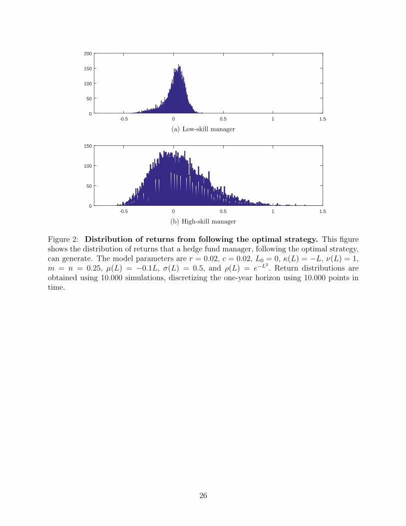
Turning next to the returns of hedge fund investors over the one-year horizon, I simulate

the returns generated by the two different managers. To do so, I discretize the one-year period

into 10.000 time steps and simulate 10.000 sample paths of returns. Figure 2 compares the

returns generated by the two managers. As we can see from Panel (a), the returns of the

bad manager are left-skewed with a small positive mean. This result is in line with the

common wisdom that liquidity provision can be seen as “picking up nickels in front of a

steamroller.” In contrast to that, the returns of the good manager exhibit a higher standard

deviation, but also a higher mean and Sharpe ratio. In particular the returns generated by

the good manager are right-skewed, indicating that there are situations where the manager

can generate significant excess returns for his investors.

4 The Data

4.1 Hedge Fund Data

The data for my analysis comes from the May 2016 version of the Lipper TASS hedge

fund database. Hedge funds report voluntarily to this database and one concern with these

self-reported returns is survivorship bias because poorly performing funds drop out of the

9

database. To mitigate this concern, I use both, live hedge funds (which are still reporting

to TASS as of the latest download) and graveyard funds (which stopped reporting). Since

the graveyard database was only established in 1994, I focus my analysis on the 1994-2014

period. Following the literature on hedge funds (see, for instance, Cao, Chen, Liang, and

Lo, 2013, Hu et al., 2013, among others), I apply three filters to the database. First, I

require funds to report returns net of fees on a monthly basis. Second, I drop hedge funds

with average AUM below 10 Mio USD. For funds that do not report in USD, I use the

appropriate exchange rate to convert AUM into USD equivalents.3 Third, I require that

each fund in my sample reports at least 24 monthly returns during my sample period.

Table 1 provides summary statistics for all hedge funds in my sample. For variables that

change over time, I first compute the time-series average and then report cross-sectional

summary statistics in the table. As we can see from the first two rows of the table, the

average fund in the database reports a positive return of 0.51% per month with a standard

deviation of 3.27. On average, funds have 147.46 million US dollar in AUM, ranging from the

minimum of 10 million up to 7797.83 million. The average fund in the database reports 90

monthly returns and is 47 months old. TASS also provides information on when a hedge fund

started reporting to the database, which enables me to compute the percentage of backfilled

returns, which is on average 43.48% with a high standard deviation of 31.35% across funds.

In my main analysis I include backfilled return observation, but I show in a robustness check

that my results are robust to excluding these observations.

The next two variables give an indication of funds’ risk of withdraws. First, the average

lockup provision of hedge funds in my sample is 2.8 months. It is worth noting that more than

half of the funds in the database do not have any lockup provision and that the high median

is driven by few outliers with extreme lockup provisions. Second, the funds’ redemption

notice period varies across funds from 0 to 365 days, with an average of 36.1 days. Finally,

median management and incentive fee of funds in my sample are 1.5% and 20%, which is

in line with the often-mentioned 2/20 rule, stating that hedge-fund managers earn a 2%

base compensation and a 20% incentive-based compensation. Furthermore, 61.49% of the

funds in my sample have a HWM provision and 22.55% of the managers invest their personal

capital in the fund.

Table 2 summarizes average hedge fund returns for the different styles and years in my

sample. As we can see from Panel A, average returns range from 0.79% per month for

long-short equity to 0.23 for funds of funds. In total, there are 3.029 funds of funds in my

sample. I run my main analysis using all 8.384 funds and show later that my results are

3Following, Cao et al. (2013), I use the returns reported in the original currency in my analysis. Adjustingreturns into USD leaves the inference unchanged.

10

robust to splitting the sample into hedge funds and funds of funds. The second-largest style

in my sample are hedge funds using long/short equity strategies with 1958 funds, followed

the event-driven style with 536 funds and multi-strategy with 524 funds.

Panel B of Table 2 shows average hedge fund returns per year. As we can see from the

table, 2008 and 2011 have been bad years for the average hedge fund in the sample with

negative average monthly returns of −1.50% in 2008 and −0.44% in 2011. It is important

to note that, although the total number of hedge funds is 8.384, the amount of hedge funds

varies significantly over time from a minimum of 711 in 1994 to 5.720 in 2009. Hence, split-

ting the overall sample of hedge funds into different subcategories can result in a relatively

small sample during some years. Later, in my analysis, I account for this observation by

sorting hedge funds into quintiles instead of deciles to insure a sufficient amount of funds

per portfolio.

4.2 Deviations from the Covered Interest Rate Parity

In this section, I construct a measure of mispricings in international money markets which

can be linked to major derivatives-dealing banks’ funding constraints.

The first criterion for constructing my measure is that the data should go back until

January 1994, which is the start date of my hedge fund panel data. This criterion rules

out several potentially interesting mispricings, such as the CDS-bond basis (Bai and Collin-

Dufresne, 2013), the CDS-index basis (Junge and Trolle, 2014), or the TIPS-treasury arbi-

trage (Fleckenstein, Longstaff, and Lustig, 2014). A second criterion is that it should be a

broad mispricing which is not specific to a particular security and instutional frictions, like

the on-the-run off-the-run spread (Krishnamurthy, 2002). Instead, the idea is to capture

similar mispricings across a variety of different assets and quantify a systemic component.

The mispricing that I use in my analysis are deviations from the covered interest rate

parity (CIP). The idea behind CIP is that investing one unit of currency A at time t in a

money-market account with interest rate rA(t, T ) should yield the same return as exchanging

this one unit of currency A into currency B, putting that money into a money-market account

with interest rate rB(t, T ), and entering a forward agreement to exchange the cashflow back

into currency A, which hedges the currency risk of the transaction. Let fwdA/B(t, T ) denote

the forward exchange rate from currency A to currency B at time t with maturity T. The

CIP then implies that the theoretical forward rate is given as:

fwd∗A/B(t, T ) := FXA/B(t)

(1 + rA(t, T )

1 + rB(t, T )

), (9)

11

where FXA/B(t) denotes the spot exchange rate from currency A to currency B and rA(t, T )

and rB(t, T ) denote the interest rate received from time t to time T in currency A and B

respectively.

The advantage of using CIP deviations is that they provide a simple and model-free proxy

of market dislocations. Furthermore, as noted by Pasquariello (2014), CIP deviations capture

a dislocation in international money markets. These dislocations are likely to be linked to

hedge fund funding conditions, since deviations typically occur when major banks experience

funding constraints.4 These funding constraints are typically passed on to customers, either

directly in form of higher margin requirements or indirectly in the form of more adverse

derivatives prices, if customers obtain leverage indirectly through derivatives.

There are a large number of possible ways to aggregate CIP deviations across different

currencies and maturities into one measure. To mitigate data-mining concerns, I choose

to construct an index of international money market “dislocations”, closely following the

procedure outlined in Pasquariello (2014). In particular, I measure CIP deviations for the

following nine currency pairs: CHF/USD, GBP/USD, EUR/USD, JPY/USD, CHF/EUR,

GBP/EUR, JPY/EUR, CHF/GBP, JPY/GBP, using spot rates and forward rates with 7,

30, 60, 90, 180, 270, and 360 days to maturity. I use Libor rates with the same maturity as

the forward rates as a proxy for the risk-free rate in the respective currency. All data for

constructing CIP deviations are obtained from the Bloomberg system. As in Pasquariello

(2014), for each currency and each maturity, I then compute the deviation from the CIP as:

CIPDi,t =

∣∣ln(FwdA/B(t, T ))− ln(Fwd∗A/B(t, T ))∣∣× 104. (10)

This procedure gives 7 different proxies for mispricings in each of the 9 different currency

pairs studied, resulting in 63 different mispricings, which are aggregated into one index:

CIPDt =

1

nt

nt∑i=1

CIPi,t, (11)

where nt is the number of available mispricings at time t.5

While measuring CIP deviations is relatively straight-forward, there are several issues

with actually implementing the strategy. As noted by Pasquariello (2014) two issues are

trading costs and funding costs. Trading costs occur because the CIP deviation measure

4For instance, Bottazzi, Luque, Pascoa, and Sundaresan (2012) and Ivashina, Scharfstein, and Stein (2015)argue that deviations from CIP can be driven by a dollar shortage of banks with international borrowingand lending.

5Note that the index becomes richer as time passes. Most notably, exchange rates involving the Euro areonly available from 1999 onwards.

12

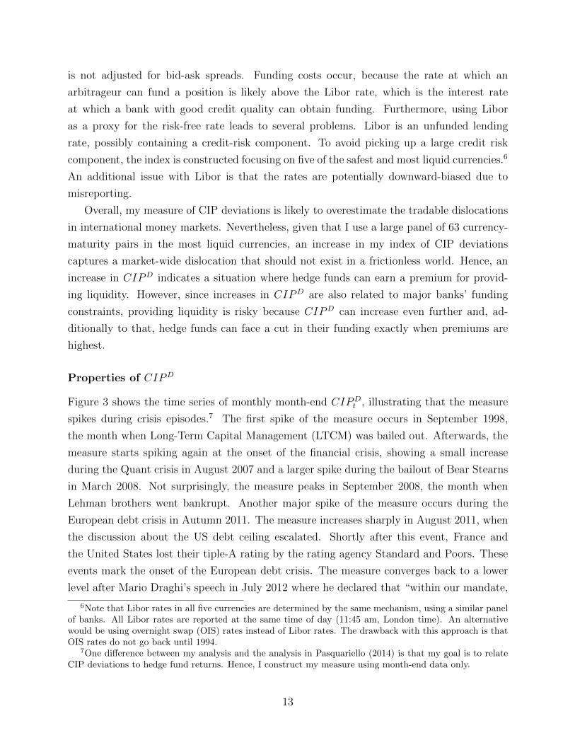
is not adjusted for bid-ask spreads. Funding costs occur, because the rate at which an

arbitrageur can fund a position is likely above the Libor rate, which is the interest rate

at which a bank with good credit quality can obtain funding. Furthermore, using Libor

as a proxy for the risk-free rate leads to several problems. Libor is an unfunded lending

rate, possibly containing a credit-risk component. To avoid picking up a large credit risk

component, the index is constructed focusing on five of the safest and most liquid currencies.6

An additional issue with Libor is that the rates are potentially downward-biased due to

misreporting.

Overall, my measure of CIP deviations is likely to overestimate the tradable dislocations

in international money markets. Nevertheless, given that I use a large panel of 63 currency-

maturity pairs in the most liquid currencies, an increase in my index of CIP deviations

captures a market-wide dislocation that should not exist in a frictionless world. Hence, an

increase in CIPD indicates a situation where hedge funds can earn a premium for provid-

ing liquidity. However, since increases in CIPD are also related to major banks’ funding

constraints, providing liquidity is risky because CIPD can increase even further and, ad-

ditionally to that, hedge funds can face a cut in their funding exactly when premiums are

highest.

Properties of CIPD

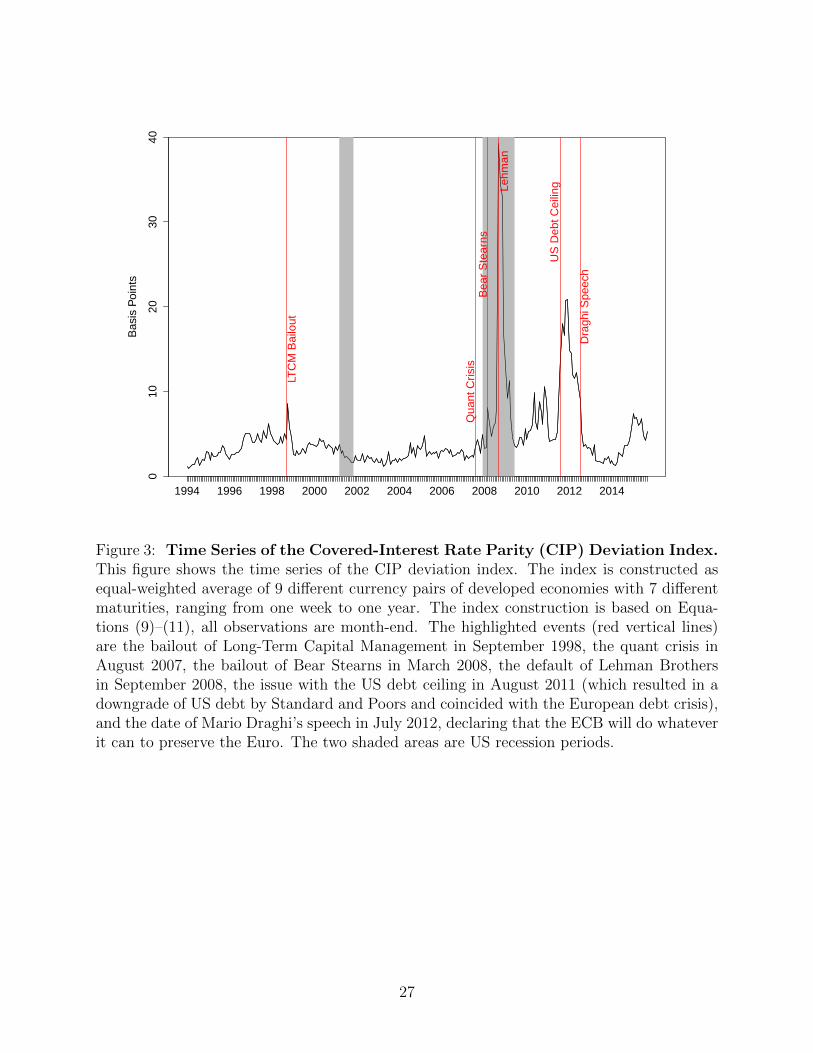
Figure 3 shows the time series of monthly month-end CIPDt , illustrating that the measure

spikes during crisis episodes.7 The first spike of the measure occurs in September 1998,

the month when Long-Term Capital Management (LTCM) was bailed out. Afterwards, the

measure starts spiking again at the onset of the financial crisis, showing a small increase

during the Quant crisis in August 2007 and a larger spike during the bailout of Bear Stearns

in March 2008. Not surprisingly, the measure peaks in September 2008, the month when

Lehman brothers went bankrupt. Another major spike of the measure occurs during the

European debt crisis in Autumn 2011. The measure increases sharply in August 2011, when

the discussion about the US debt ceiling escalated. Shortly after this event, France and

the United States lost their tiple-A rating by the rating agency Standard and Poors. These

events mark the onset of the European debt crisis. The measure converges back to a lower

level after Mario Draghi’s speech in July 2012 where he declared that “within our mandate,

6Note that Libor rates in all five currencies are determined by the same mechanism, using a similar panelof banks. All Libor rates are reported at the same time of day (11:45 am, London time). An alternativewould be using overnight swap (OIS) rates instead of Libor rates. The drawback with this approach is thatOIS rates do not go back until 1994.

7One difference between my analysis and the analysis in Pasquariello (2014) is that my goal is to relateCIP deviations to hedge fund returns. Hence, I construct my measure using month-end data only.

13

the ECB is ready to do whatever it takes to preserve the euro. And believe me, it will be

enough.”8

I study the relationship between ∆CIPDt and other commonly used proxies of market

uncertainty and funding illiquidity in Table 3. Changes in CIPDt are strongly related to

changes in the TED spread, which is the difference between the 3-month US Libor rate

and the 3-month US treasury yield and a common proxy for market liquidity, as well as to

changes in the VIX index, which is the implied volatility of the S&P 500 and a common

measure of market uncertainty.

4.3 Hedge Fund Risk Factors and their Relation to CIPD

I now describe the seven most commonly used hedge fund risk factors, which were proposed

by Fung and Hsieh (2004) and investigate their relationship to ∆CIPt afterwards. The

first two factors are related to stock markets, capturing US stock market excess returns

(MKT) and the returns from a small-minus big portfolio (SMB). I use the first two Fama-

French factors, obtained from Kenneth French’s website, to proxy for these two factors.

Furthermore, Fung and Hsieh (2001) suggest the monthly change in the ten-year US treasury

constant maturity yield (YLD) and the monthly change in the Moody’s Baa yield less ten-

year Treasury constant maturity yield (BAA) as risk factors capturing interest-rate risk and

credit risk. I obtain data for these two factors from the Bloomberg system. Finally, Fung

and Hsieh also propose three trend-following factors one for bonds (BD), one for currencies

(FX), and one commodities (COM), which are obtained from David Hsiesh’s website.9

Table 3 shows the correlation between changes in CIP deviations and the seven hedge

fund risk factors. As we can see, the correlation is generally low. Only the correlation

between YLD and BAA, as well as the correlation between FX and COM is above 30%. The

correlation between ∆CIPDt and the other seven factors is weaker than 15%, indicating that

CIP deviations are not captured by the other factors.

Sadka (2010) points out that YLD and BAA are not capturing excess returns and are

therefore not suitable to compute risk-adjusted hedge fund returns. I therefore follow Sadka

(2010) and replace these two factors with tradable factors in my performance analysis in

the following section. In particular, I obtain the Merril Lynch treasury bond index with

7-10 years to maturity and the a corporate bond index of BBB-rated bonds with 7-10 years

to maturity from the Bloomberg system. I compute the returns on both indices and use

excess return of the treasury bond index over the one-month treasury bill rate as a tradable

8See https://www.ecb.europa.eu/press/key/date/2012/html/sp120726.en.html for a verbatim ofthe speech.

9These factors are available under: https://faculty.fuqua.duke.edu/~dah7/HFData.htm

14

proxy for the YLD factor. The two variables have a correlation of -69%. Similarly, I use the

difference between the returns from the BBB-rated corporate bond index and the treasury

bond index as a proxy for the BAA factor. The correlation between these two variables is

-76%. In the following I replace YLD and BAA with the two tradable factors to compute

risk-adjusted returns.

5 Results

Methodology

To test my hypothesis that hedge funds following funding-risky strategies can severely under-

perform hedge funds who do not rely on funding-risky strategies to generate their returns, I

sort hedge funds into deciles based on their loading on CIPDt . Every month, for each fund i, I

run a regression of hedge fund excess returns over the past 36 months on ∆CIPD, controlling

for excess returns of the (stock) market portfolio:10

RExct,i = α + βCIP∆CIPD

t + βMktRMktt + εt. (12)

Based on βCIP , I then put each hedge fund in one decile portfolio, where funds in the first

portfolio have the most negative βCIP while funds in the last portfolio have the highest

βCIP . The decile portfolios are rebalanced every month, repeating the sorting procedure.

The first portfolio has the strongest loading on ∆CIPDt , while portfolio 10 has the weakest

loading. Note that a strong loading on ∆CIPDt corresponds to a significant negative beta

since increases in deviations from the CIP correspond lower returns for hedge funds following

these strategies while a weak loading corresponds to an insignificant beta close to zero.

Main Results

I illustrate the results from this sorting procedure graphically in Figure 4, where I plot the

monthly risk-adjusted returns of the 10 portfolios, controlling for the risk factors proposed

by Fung and Hsieh (2004). As we can see, funds in portfolio 10, which have the weakest

loading on CIP deviations have a monthly risk-adjusted return of 0.46%, which corresponds

to an annual alpha of 5.52%. Strikingly, funds with a weak loading are outperforming funds

with a strong loading on ∆CIPDt by more than 0.46% per month. Furthermore, the red

10Controlling only for returns of the market portfolio in the first step has been common practice in theliterature (see Sadka, 2010, Hu et al., 2013 for hedge funds, or Ang, Hodrick, Xing, and Zhang, 2006, amongmany others, for stocks). In unreported robustness checks, I also experimented with controlling for the othersix Fung Hsieh risk factors as well as with only using the past 24 months of observations, which both led toqualitatively similar results.

15

dots in the figure show Newey-West t-statistics of the respective portfolios and indicate that

the results are not only economically but also statistically significant. The risk-adjusted

return of the low-loading portfolio is significant at a 1% level with a t-statistic of 3.5 and the

risk-adjusted return of the difference portfolio that is long the low-loading decile and short

the high-loading decile is significant at a 5% level with a t-statistic of 2.18%.

More detailed results with the exact parameter estimates are reported in Table 5. I

emphasize the following three observations from Table 5. First, excess returns of the hedge

funds in the different deciles increase almost monotonically as the loading on ∆CIPD weak-

ens. However, the difference between top and bottom decile is not statistically significant.

Second, the post-ranking betas of the 10 portfolios are increasing almost monotonically,

even after controlling for the 7 Fung-Hsieh risk factors. The difference portfolio also has a

statistically significant loading on ∆CIPD (t-statistic of 1.95). This relatively small differ-

ence in post-sorting betas can be attributed to controlling for the 7 other risk factors. In

an unreported robustness check, I also computed the post-sorting betas only controlling for

the return on the market portfolio, which gave a βCIP of 0.16 for the difference portfolio (t-

statistic of 3.29). Third, the explanatory power of CIPDt and the other risk factors decreases

almost monotonically from top to bottom portfolio as well. One possible explanation for this

observation is that fund managers who are able to avoid loading on CIPDt are also better in

avoiding other common risk factors. In that sense, my finding is related to Titman and Tiu

(2011) who show that hedge funds with low loading on known risk factors outperform funds

with high loadings.

A Closer Look at the Time Series

To get a better understanding of the decile excess returns, Figure 5 plots the time series of

cumulative excess returns of the top and bottom decile. As we can see, the returns from the

top decile (strong loading on CIPDt ) are more volatile and generally lower than those of the

low loading decile. More specifically, the high-loading portfolio suffers large losses around

the LTCM crisis in 1998, around the default of Lehman brothers in 2008, and during the

European debt crisis in 2011/2012. In contrast to that, the low-loading portfolio provides

stable returns during crisis periods, with moderate losses during the 2008 crisis. Hence,

Figure 5 indicates that the high risk-adjusted returns from funds with a weak loading on

CIP deviations are mainly earned during crisis periods and that the high difference between

funds with a strong and a weak loading mainly come from episodes of financial distress.

To provide some more formal evidence for this results, I split my sample into periods of

crisis and normal times. First, I simply use anecdotal evidence about crisis periods, thereby

identifying 18 months which are plausibly periods with severe funding constraints for hedge

16

fund managers. The crisis periods are are August-September 1998 (the period of the Russian

debt crisis and the LTCM bailout), August-October 2007 (the months of the quant crisis),

August 2008 - January 2009 (the time around the default of Lehman brothers), August -

December 2011 (the first part of the European debt crisis), and April - May 2012 (the second

part of the European debt crisis). As we can see from Panel (I) of Table 6, monthly excess

returns of the difference portfolio that is long hedge funds with a weak loading on ∆CIPDt

(bottom decile) and short hedge funds with a strong loading on ∆CIPDt (top decile) during

crisis periods are 3.23% which are statistically significant at a 1% level. Similarly risk-

adjusted returns of the difference portfolio are 1.89% and also highly statistically significant.

In contrast, the returns and risk-adjusted returns of the difference portfolio are insignificant

during normal periods.

To test the difference between crisis and non-crisis episodes more formally, I follow Teo

(2011) and split the sample period based on the level of the TED spread and define crisis

periods as episodes where the TED spread is above its 80% quantile and non-crisis periods as

episodes where the TED spread is below its 20% quantile. The results are qualitatively similar

to (I), indicating that the difference portfolio is delivering statistically significant returns

during times of financial distress, but insignificant returns during quiet times. Similarly, I

split the sample period into times where average stock returns of the 16 largest dealer banks

are below their 20% quantile (crisis episodes) and episodes where returns are above their

80% quantile. For this split, the results are qualitatively similar but less significant.11

Finally, I provide an overview of the characteristics of the funds in the different decile

portfolios in Table 7. As we can see from the table, funds in the top and bottom decile

have very similar characteristics, while there is a tendency for funds in portfolios 4-6 to

have slightly different characteristics and a different allocation between styles. Most notably,

portfolios 3-7 consist of almost 50% funds of funds while top and bottom portfolio only consist

of 11% funds of funds. I formally test whether different characteristics can be responsible

for my finding in Section 5.2, where I run Fama and MacBeth (1973) regressions, controlling

for fund characteristics like lockup provision and assets under management as well as hedge

fund style.

5.1 Results For Different Subsamples

To shed further light on my findings, I now split the entire hedge fund sample that I have

used so far into various different subsamples and repeat my analysis. To ensure a sufficient

number of funds in each quantile, I follow Teo (2011) and only form quintile portfolios.

11One possible explanation is that stock returns do not capture dealer-banks constraints appropriately. Inthe next version of this paper I plan on using EDF data to quantify periods of financial distress.

17

Fund-Specific Funding Risk

To investigate the role of hedge fund specific funding risk, I perform the following three tests.

First, I split the sample into hedge funds that are currently performing at their HWM and

funds that are currently under water. The idea behind this split is that hedge funds that have

suffered drawdowns are facing an additional risk of getting their funding cut by their prime

broker. To approximate drawdowns from the HWM, I use the ratio X between current NAV

of the fund and maximium NAV over the history of the fund. Every month t, I then split

the sample into one part that is currently at its HWM, where Xt−1 = 1, and one part that

has suffered drawdowns Xt−1 < 1. I rebalance the two portfolios on a monthly basis. Panels

(a) and (b) of Figure 6 illustrate the results. As we can see from the figure, hedge funds that

are currently at their HWM generally outperform hedge funds that suffered drawdowns by a

large margin.In both sub-samples, hedge funds with a high loading on CIPD underperform

funds with a low loading. However, the difference is smaller and less significant for funds

that did not suffer drawdowns. In particular the difference portfolio that is long hedge funds

with a weak loading and short hedge funds with a strong loading generates a monthly alpha

of 0.3% for funds that did not suffer drawdowns while it generates a monthly alpha of 0.4%

for funds that did suffer drawdowns.

Second, I use the hedge fund redemption notice period as a fund-specific proxy for funding

liquidity. Hedge funds with longer redemption notice periods are less susceptible for equity

withdraws in times of financial distress than funds with shorter redemption notice periods.

Even thought this is a proxy for the equity part of the balance sheet, funding obtained from

prime brokers can be related to equity withdraws. In line with Aragon (2007), Panels (c)

and (d) of Figure 6 show that hedge funds with longer redemption notice periods tend to

outperform funds with shorter redemption notice periods. Additional to that, we can see

from the two figures that the effect is less pronounced for funds with longer redemption

notice periods. In particular, the difference portfolio that is long hedge funds a weak loading

on CIP deviations and short funds with a strong loading on CIP deviations generates a

monthly alpha of 0.3% for funds with longer redemption notice periods and an alpha of 0.4%

for funds with shorter redemption notice periods.

Third, I divide the sample into funds with lockup provision and funds without lockup

provision. Again, this is a proxy for the equity side of funding risk. The results of this split

are exhibited in panels (e) and (f) of Figure 6. As before, funds with longer lockup periods

are generally performing better than funds with shorter lockup periods and the effect is

more pronounced for funds without lockup provision. The difference portfolio for funds with

lockup provision generates a monthly alpha of 0.22% while the difference portfolio for funds

without lockup provision generates a monthly alpha of 0.38%.

18

Different Hedge Fund Styles

I next address the question of whether my results hold for funds with different investment

styles. To that end, I split my sample into three different style categories, funds of funds

(total of 3017 funds), long/short equity (total of 1953 funds), and funds from the remaining

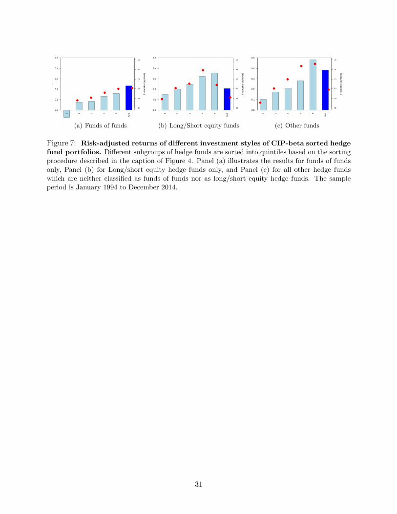
categories (total of 3395 funds). Panels (a), (b), and (c) of Figure 7 illustrate the results and

show that the results are qualitatively similar for different styles. Panel (a) shows that funds

of funds with a high loading on CIPD are doing exceptionally poor compared to funds with a

high loading on CIPD in the other categories. One possible explanation for this observation

is that funds of funds load indirectly on CIPD by investing in hedge funds who load on

it. When funding becomes scarce, their investments underperform and they face funding

constraints of their own which amplifies the mechanism. For long/short equity funds the

results is weakest.

5.2 Robustness Checks

In this section, I present the results from running Fama and MacBeth (1973) regressions,

where I control for several fund characteristics. I repeat this analysis for three modifications

of the database to address common issues with hedge fund data. First, to run Fama-MacBeth

regressions, I compute the alpha of each hedge fund, using the following equation:

αi,t = RExci,t − (βMkt

i RMktt + βSMB

i RSMBt + βY LDi RY LD

t + βBAAi RBAAt

+ βBDi RBDt + βFXi RFX

t + βCOMi RCOMt ), (13)

where fund-specific betas are computed using the entire time series of hedge fund returns. I

then follow the common practice (see, e.g. Klebanov (2008) or Hu et al. (2013)) and assign

portfolio βCIP for the regression. In particular, a fund that is in portfolio i at time t and in

portfolio j at time t + 1 gets βCIP of portfolio i at time t and βCIP of portfolio j at time

t+ 1. I then run the following regression:

αi,t = γ0 + γ1βCIPi,t−1 + γ2Controlsi + ε (14)

The results of this regression without control variables are exhibited in the first row of Table

8. As we can see, the loading on CIP deviations is statistically significant in explaining the

cross-section of hedge fund returns. As a second step I control for the hedge fund’s age, size

(proxied by the logarithm of its assets under management), its redemption frequency, the

redemption notice period, the lockup period, and its style (by adding style dummies). The

effect of βCIP is still statistically significant at a 5% level after adding these control variables.

19

Biases in Reported Hedge Fund Data

As a next step, I address the most common biases in hedge fund data. As mentioned in

Section 4.1, hedge funds report their returns voluntarily to the Tass database. Fung and

Hsieh (2000) explain that there are several biases in these self-reported data. The first

concern, which is survivorship bias, can be mitigated by using both, hedge funds that are

currently reporting to the database and funds that have stopped reporting to the database

(which I do in my analysis). The second concern is selection bias, meaning that funds only

report to the database if their returns are high. This concern is more difficult to address, but

Fung and Hsieh (2001) argue that this concern is least relevant for funds of funds. Hence,

Panel (c) of Figure 7 mitigates this concern. Another concern described by Fung and Hsieh

(2001) is backfilling bias. A fund that starts reporting to the database can also report

historical returns. Clearly, only funds with high past returns would do that which biases

returns upwards.

Hence, the first main issue with the data is a selection bias. As explained in Section

4.1, the Tass database provides the date at which a fund started reporting to the database.

To check if my results are robust to backfilled bias, I drop all backfilled observations. As

illustrated in Table 1, on average 43% of hedge fund returns are backfilled. Repeating the

analysis without backfilled returns leads to significantly lower alphas but qualitatively similar

results. For brevity, I only report the results from a Fama-MacBeth regression where I drop

backfilled observations.12 The results of this analysis are presented in the third row of Table

8. While the size of the intercept drops sharply, the coefficient for βCIP decreases from 4.2

to 3.8 and is still statistically significant at a 5% level.

Another concern about hedge fund data is return smoothing. Hedge funds holding illiquid

securities might report returns with a lag (see Asness, Krail, and Liew (2001) and Getmansky,

Lo, and Makarov (2004)). Getmansky et al. (2004) propose an econometric technique to un-

smooth hedge fund returns. I use their technique to obtain un-smoothed returns Rt by

estimating the following model:

Rot = θ0Rt + θ1Rt−1 + θ2Rt−2, (15)

where R0t is the observed hedge fund return at time t and

∑2i=0 θi = 1. I then repeat my

analysis using un-smoothed returns and report the results in the fourth row of Table 8. As we

can see from the table, βCIP is still statistically significant at a 5% level for this specification.

Finally, the voluntary nature of reporting hedge fund returns can also cause hedge funds

with poor past performance to stop reporting to the database. To address this concern, I

12Regression results for top, bottom, and difference portfolio will be reported in an online appendix...

20

replace the last reported return of each hedge fund in the database with −20%.13 The results

of this robustness check are reported in the final row of Table 8. As we can see from this

row, βCIP is still significant at a 5% level and the size of the coefficient is almost unchanged,

compared to the base case.

6 Conclusion

I develop a theory in which a hedge fund manager can invest in an arbitrage position and an

alpha-generating strategy. If the arbitrage spread is strongly correlated with the manager’s

own funding risk, it is optimal to avoid loading on the arbitrage mispricing. To confirm this

theory, I construct a measure of mispricings in international money markets and show that

this measure is highly correlated to other proxies of funding liquidity. In line with my theory,

I find that hedge funds with a lower loading on these mispricings outperform funds with a

higher loading.

13The inference for βCIP remains unchanged if I use more negative numbers like −50%.

21

References

Abreu, D. and M. K. Brunnermeier (2003). Bubbles and crashes. Econometrica 71 (1), 173–204.

Ang, A., S. Gorovyy, and G. B. Van Inwegen (2011). Hedge fund leverage. Journal of Financial Eco-

nomics 102 (1), 102–126.

Ang, A., R. J. Hodrick, Y. Xing, and X. Zhang (2006). The cross-section of volatility and expected returns.

The Journal of Finance 61 (1), 259–299.

Aragon, G. O. (2007). Share restrictions and asset pricing: Evidence from the hedge fund industry. Journal

of Financial Economics 83 (1), 33–58.

Asness, C. S., R. Krail, and J. M. Liew (2001). Do hedge funds hedge? Available at SSRN 252810 .

Bai, J. and P. Collin-Dufresne (2013). The cds-bond basis. In AFA 2013 San Diego Meetings Paper.

Basak, S., A. Pavlova, and A. Shapiro (2007). Optimal asset allocation and risk shifting in money manage-

ment. Review of Financial Studies 20 (5), 1583–1621.

Ben-David, I., F. Franzoni, and R. Moussawi (2012). Hedge fund stock trading in the financial crisis of

2007–2009. Review of Financial Studies 25 (1), 1–54.

Bottazzi, J.-M., J. Luque, M. Pascoa, and S. M. Sundaresan (2012). Dollar shortage, central bank actions,

and the cross currency basis. Central Bank Actions, and the Cross Currency Basis (October 27, 2012).

Brunnermeier, M. and S. Nagel (2004). Hedge funds and the technology bubble. The Journal of Fi-

nance 59 (5), 2013–2040.

Brunnermeier, M. K. and L. H. Pedersen (2009). Market liquidity and funding liquidity. Review of Financial

studies 22 (6), 2201–2238.

Cao, C., Y. Chen, B. Liang, and A. W. Lo (2013). Can hedge funds time market liquidity? Journal of

Financial Economics 109 (2), 493–516.

Christoffersen, S. K., D. K. Musto, and B. Yilmaz (2015). High water marks in competitive capital markets.

Dai, Q. and S. M. Sundaresan (2011). Risk management framework for hedge funds: role of funding and

redemption options on leverage. Available at SSRN 1439706 .

Drechsler, I. (2014). Risk choice under high-water marks. Review of Financial Studies, hht081.

Fama, E. F. and J. D. MacBeth (1973). Risk, return, and equilibrium: Empirical tests. The Journal of

Political Economy , 607–636.

Fleckenstein, M., F. A. Longstaff, and H. Lustig (2014). The tips-treasury bond puzzle. The Journal of

Finance 69 (5), 2151–2197.

Frazzini, A. and L. H. Pedersen (2014). Betting against beta. Journal of Financial Economics 111 (1), 1–25.

22

Fung, W. and D. A. Hsieh (2000). Performance characteristics of hedge funds and commodity funds: Natural

vs. spurious biases. Journal of Financial and Quantitative Analysis 35 (03), 291–307.

Fung, W. and D. A. Hsieh (2001). The risk in hedge fund strategies: Theory and evidence from trend

followers. Review of Financial studies 14 (2), 313–341.

Fung, W. and D. A. Hsieh (2004). Hedge fund benchmarks: A risk-based approach. Financial Analysts

Journal 60 (5), 65–80.

Garleanu, N. and L. H. Pedersen (2011). Margin-based Asset Pricing and Deviations from the Law of One

Price. Review of Financial Studies 24 (6), 1980–2022.

Getmansky, M., A. W. Lo, and I. Makarov (2004). An econometric model of serial correlation and illiquidity

in hedge fund returns. Journal of Financial Economics 74 (3), 529–609.

Goetzmann, W. N., J. E. Ingersoll, and S. A. Ross (2003). High-water marks and hedge fund management

contracts. The Journal of Finance 58 (4), 1685–1718.

Gromb, D. and D. Vayanos (2002). Equilibrium and welfare in markets with financially constrained arbi-

trageurs. Journal of Financial Economics 66 (2-3), 361–407.

Gromb, D. and D. Vayanos (2015). The dynamics of financially constrained arbitrage. Technical report,

National Bureau of Economic Research.

Hu, G. X., J. Pan, and J. Wang (2013). Noise as information for illiquidity. The Journal of Finance 68 (6),

2341–2382.

Ivashina, V., D. S. Scharfstein, and J. C. Stein (2015). Dollar funding and the lending behavior of global

banks. The Quarterly Journal of Economics 130 (3), 1241–1281.

Junge, B. and A. B. Trolle (2014). Liquidity risk in credit default swap markets. Swiss Finance Institute

Research Paper (13-65).

Klebanov, M. M. (2008). Betas, characteristics and the cross-section of hedge fund returns. Characteristics

and the Cross-Section of Hedge Fund Returns (January 7, 2008).

Krishnamurthy, A. (2002). The bond/old-bond spread. Journal of Financial Economics 66 (2), 463–506.

Lan, Y., N. Wang, and J. Yang (2013). The economics of hedge funds. Journal of Financial Eco-

nomics 110 (2), 300–323.

Liu, J. and F. A. Longstaff (2004). Losing money on arbitrage: Optimal dynamic portfolio choice in markets

with arbitrage opportunities. Review of Financial Studies 17 (3), 611–641.

Liu, X. and A. S. Mello (2011). The fragile capital structure of hedge funds and the limits to arbitrage.

Journal of Financial Economics 102 (3), 491–506.

Mitchell, M. and T. Pulvino (2012). Arbitrage crashes and the speed of capital. Journal of Financial

Economics 104 (3), 469–490.

23

Pangeas, S. and M. M. Westerfield (2009). High watermarks: High risk appetites? hedge fund compensation

and portfolio choice. Journal of Finance.

Pasquariello, P. (2014). Financial market dislocations. Review of Financial Studies 27 (6), 1868–1914.

Pastor, L. and R. F. Stambaugh (2003). Liquidity risk and price discovery. Journal of Political Econ-

omy 111 (3), 642–685.

Pedersen, L. H. (2015). Efficiently Inefficient: How Smart Money Invests and Market Prices Are Determined.

Princeton University Press.

Sadka, R. (2006). Momentum and post-earnings-announcement drift anomalies: The role of liquidity risk.

Journal of Financial Economics 80 (2), 309–349.

Sadka, R. (2010). Liquidity risk and the cross-section of hedge-fund returns. Journal of Financial Eco-

nomics 98 (1), 54–71.

Shleifer, A. and R. W. Vishny (1997). The limits of arbitrage. The Journal of Finance 52 (1), 35–55.

Sotes-Paladino, J. M. and F. Zapatero (2015). Riding the bubble with convex incentives. Marshall School

of Business Working Paper No. FBE 6.

Teo, M. (2011). The liquidity risk of liquid hedge funds. Journal of Financial Economics 100 (1), 24–44.

Titman, S. and C. Tiu (2011). Do the best hedge funds hedge? Review of Financial Studies 24 (1), 123–168.

24

Figures and Tables

0 0.2 0.4 0.6 0.8 1 1.2 1.4 1.6 1.8 2-0.6

-0.4

-0.2

0

0.2

0.4

0.6

0.8

1

1.2 Investment in Asset aInvestment in Asset b

(a) Low-skill manager

0 0.2 0.4 0.6 0.8 1 1.2 1.4 1.6 1.8 2-0.6

-0.4

-0.2

0

0.2

0.4

0.6

0.8

1

1.2 Investment in Asset aInvestment in Asset b

(b) High-skill manager

Figure 1: Optimal risky asset holdings of different managers. This figure shows theoptimal investments in the alpha-generating strategy (asset a) and the funding-risky strategy(asset b) of a manager with low skill and high skill. The model parameters are r = 0.02,c = 0.02, L0 = 0, κ(L) = −L, ν(L) = 1, m = n = 0.25, µ(L) = −0.1L, σ(L) = 0.5, andρ(L) = e−L

2.

25

-0.5 0 0.5 1 1.50

50

100

150

200

(a) Low-skill manager

-0.5 0 0.5 1 1.50

50

100

150

(b) High-skill manager

Figure 2: Distribution of returns from following the optimal strategy. This figureshows the distribution of returns that a hedge fund manager, following the optimal strategy,can generate. The model parameters are r = 0.02, c = 0.02, L0 = 0, κ(L) = −L, ν(L) = 1,m = n = 0.25, µ(L) = −0.1L, σ(L) = 0.5, and ρ(L) = e−L

2. Return distributions are

obtained using 10.000 simulations, discretizing the one-year horizon using 10.000 points intime.

26

1994 1996 1998 2000 2002 2004 2006 2008 2010 2012 2014

010

2030

40

Bas

is P

oint

s

LTC

M B

ailo

ut

Qua

nt C

risis

Lehm

an

US

Deb

t Cei

ling

Dra

ghi S

peec

h

Bea

r S

tear

ns

Figure 3: Time Series of the Covered-Interest Rate Parity (CIP) Deviation Index.This figure shows the time series of the CIP deviation index. The index is constructed asequal-weighted average of 9 different currency pairs of developed economies with 7 differentmaturities, ranging from one week to one year. The index construction is based on Equa-tions (9)–(11), all observations are month-end. The highlighted events (red vertical lines)are the bailout of Long-Term Capital Management in September 1998, the quant crisis inAugust 2007, the bailout of Bear Stearns in March 2008, the default of Lehman Brothersin September 2008, the issue with the US debt ceiling in August 2011 (which resulted in adowngrade of US debt by Standard and Poors and coincided with the European debt crisis),and the date of Mario Draghi’s speech in July 2012, declaring that the ECB will do whateverit can to preserve the Euro. The two shaded areas are US recession periods.

27

1 2 3 4 5 6 7 8 9 10

10−

1

Fung Hsieh AlphasM

onth

ly A

lpha

0.0

0.1

0.2

0.3

0.4

●

●

● ● ●

●●

● ●

●

●

01

23

4

T−

stat

istic

s (s

ymbo

ls)

Figure 4: Risk-adjusted returns of CIP-beta sorted hedge fund portfolios. Eachmonth hedge funds are sorted into 10 equally weighted portfolios according to their historicalbeta to changes in the covered interest rate parity (CIP) deviation index, constructed inSection 4.2. Funds in portfolio 1 have the strongest loading on changes in the CIP deviationindex (the most negative beta), funds in portfolio 10 have the weakest loading (beta closeto zero). The CIP beta is calculated using a regression of monthly portfolio returns onthe market portfolio and changes in the CIP deviation index, using the 36 months priorto portfolio formation. Portfolio returns begin January 1997. The bars represent monthlyportfolio alphas calculated using the 7 Fung-Hsieh factors, where credit and term factors arereplaced by factor-mimicking tradable portfolios. The red dots are Newey-West t-statisticsof the respective alphas. The blue bar displays the alpha of a portfolio that is long hedgefunds in portfolio 10 and short hedge funds in portfolio 1. The sample period is January1994 to December 2014, including all 8384 hedge funds from the Tass database.

28

1997 1999 2001 2003 2005 2007 2009 2011 2013

1.0

1.5

2.0

2.5

3.0

3.5

Hedge Fund Returns

Cum

ulat

ive

Ret

urn

Strong LoadingWeak Loading

Figure 5: Cumulative excess returns from investing in high and low loading funds. Thisfigure shows the cumulative excess returns of hedge funds with a strong loading (solid line) and lowweak loading (dashed line) on the covered interest rate parity (CIP) deviation index, constructedin Section4.2. See the caption of Figure 4 for a description of the sorting procedure. The high (low)loading portfolio is the first (tenth) decile portfolio.

29

1 2 3 4 5

5−1

Mon

thly

Alp

ha

0.0

0.1

0.2

0.3

0.4

0.5

0.6

0.7

●

●●

●

●

●

01

23

45

67

T−

stat

istic

s (s

ymbo

ls)

(a) No Drawdown (X = 1)

1 2 3 4 5

5−1

Mon

thly

Alp

ha

0.0

0.1

0.2

0.3

0.4

0.5

0.6

0.7

●

● ●

●● ●

01

23

45

67

T−

stat

istic

s (s

ymbo

ls)

(b) Drawdown (X < 1)

1 2 3 4 5

5−1

Mon

thly

Alp

ha

0.0

0.1

0.2

0.3

0.4

●

●

●

●

●

●

01

23

4

T−

stat

istic

s (s

ymbo

ls)

(c) Longer than median redemption

1 2 3 4 5

5−1

Mon

thly

Alp

ha

0.0

0.1

0.2

0.3

0.4

●

● ●

●

●

●

01

23

4

T−

stat

istic

s (s

ymbo

ls)

(d) Median or below redemption

1 2 3 4 5

5−1

Mon

thly

Alp

ha

0.0

0.1

0.2

0.3

0.4

0.5

● ● ●

●

●

●

01

23

45

T−

stat

istic

s (s

ymbo

ls)

(e) Above median Lockup

1 2 3 4 5

5−1

Mon

thly

Alp

ha

0.0

0.1

0.2

0.3

0.4

0.5

●

●●

●

●

●0

12

34

5

T−

stat

istic

s (s

ymbo

ls)

(f) Median or below Lockup

Figure 6: Risk-adjusted returns of different subgroups of CIP-beta sorted hedge fundportfolios. Different subgroups of hedge funds are sorted into quintiles based on the sortingprocedure described in the caption of Figure 4. Panels (a) and (b) compare hedge funds that havenot suffered any drawdowns in the previous month (HWM/NAV = 1) with hedge funds that havesuffered drawdowns in the previous month (HWM/NAV = 1). Panels (c) and (d) compare hedgefunds which offer redemption terms for their equity holders below the median with hedge fundsthat offer redemption terms above the median. Panels (e) and (f) compare hedge funds with lockupperiod above the median to hedge funds with lockup period below the median. The sample periodis January 1994 to December 2014.

30

1 2 3 4 5

5−1

Mon

thly

Alp

ha

0.0

0.1

0.2

0.3

0.4

0.5

●

●●

●

● ●

01

23

45

T−

stat

istic

s (s

ymbo

ls)

(a) Funds of funds

1 2 3 4 5

5−1

Mon

thly

Alp

ha

0.0

0.1

0.2

0.3

0.4

0.5

●

●

●

●

●

●

01

23

45

T−

stat

istic

s (s

ymbo

ls)

(b) Long/Short equity funds

1 2 3 4 5

5−1

Mon

thly

Alp

ha

0.0

0.1

0.2

0.3

0.4

0.5

●

●

●

●●

●

01

23

45

T−

stat

istic

s (s

ymbo

ls)

(c) Other funds

Figure 7: Risk-adjusted returns of different investment styles of CIP-beta sorted hedgefund portfolios. Different subgroups of hedge funds are sorted into quintiles based on the sortingprocedure described in the caption of Figure 4. Panel (a) illustrates the results for funds of fundsonly, Panel (b) for Long/short equity hedge funds only, and Panel (c) for all other hedge fundswhich are neither classified as funds of funds nor as long/short equity hedge funds. The sampleperiod is January 1994 to December 2014.

31

Table 1: Hedge Fund Summary Statistics. This table provides summary statistics of averagehedge fund returns in the Tass database as well as key fund characteristics over the 1994–2014period. X is the ratio between current net-asset value (NAV) and the maximum NAV over the pastmonths. AUM is the fund’s assets under management and converted in USD for funds that reportin a different currency (using the appropriate exchange rate). Reporting and Age are the numberof monthly return observations and the average number of past return observations respectively.Backfilled gives the percentage of backfilled return observations. Lockup period is the number ofmonths that a fund can lockup investor capital. Notice is the number of days that investors haveto notice the manager before withdrawing capital from the fund. HWM and Personal Captial areindicator variables. HWM equals one if the fund manager’s compensation is linked to a high-water-mark and Personal Capital equals one if the manager invests personal capital in the fund.

Mean SD Min Median Max N

Return (mean) 0.51 0.72 -7.04 0.45 7.15 8384Return (SD) 3.27 2.64 0 2.45 33.95 8384

X 0.93 0.08 0.19 0.96 1 8384AUM (mio USD) 147.46 322.36 10 56.25 7878.71 8384

Reporting (Months) 90.68 51.69 24 78 252 8384Age (Months) 47.16 31.49 11.5 39.5 365 8384Backfilled (%) 43.48 31.52 0 37.21 100 8384

Lockup Period (Months) 2.8 6.45 0 0 90 8384Redemption Notice (Months) 36.11 33.64 0 30 365 8384

Management Fee 1.43 0.67 0 1.5 22 8330Incentive Fee 13.94 8.35 0 20 50 8284

HWM (%) 61.49 - - - - 8330Personal Capital (%) 22.55 - - - - 8384

32

Table 2: Summary Statistics of Hedge Fund Returns. This table provides summary statis-tics of average hedge fund returns for different investment styles (Panel A) and different periods(Panel B).

Mean SD Min Meadian Max N

Panel A: Summy statistics of the indicated variables for all hedge funds

Convertible Arbitrage 0.40 0.56 -1.24 0.52 1.81 199.00Emerging Markets 0.71 0.90 -3.14 0.67 5.58 492.00

Equity Market Neutral 0.42 0.60 -2.88 0.37 5.09 351.00Event Driven 0.78 0.76 -3.92 0.71 6.93 536.00

Fixed Income Arbitrage 0.43 0.73 -3.01 0.50 2.19 236.00Fund of Funds 0.23 0.50 -5.20 0.27 3.07 3029.00Global Macro 0.58 0.82 -6.68 0.56 5.64 287.00

Long/Short Equity Hedge 0.79 0.79 -5.77 0.72 7.15 1958.00Managed Futures 0.63 0.68 -3.99 0.55 3.99 411.00

Multi-Strategy 0.51 0.79 -7.04 0.48 4.92 524.00Other 0.62 0.78 -2.13 0.59 5.80 361.00

Panel B: Hedge fund returns in different style categories

1994 0.12 1.63 -10.62 0.14 10.94 711.001995 1.45 1.70 -6.58 1.27 16.80 918.001996 1.62 1.50 -4.03 1.37 11.25 1165.001997 1.54 1.61 -12.34 1.38 18.96 1398.001998 0.47 2.25 -12.85 0.57 15.66 1639.001999 2.28 3.10 -9.99 1.58 41.37 1966.002000 0.99 2.14 -23.07 0.96 23.22 2271.002001 0.62 1.99 -21.83 0.55 48.43 2695.002002 0.32 1.37 -17.05 0.27 15.91 3200.002003 1.33 1.69 -14.47 0.93 40.23 3791.002004 0.73 0.93 -5.34 0.58 10.98 4490.002005 0.78 1.22 -9.44 0.61 27.68 5137.002006 0.96 1.14 -6.14 0.81 23.72 5541.002007 0.87 1.46 -15.46 0.69 43.38 5720.002008 -1.50 2.45 -22.23 -1.39 22.37 5640.002009 1.14 3.65 -100.00 0.83 188.45 5036.002010 0.61 1.36 -34.55 0.50 26.85 4532.002011 -0.44 1.30 -23.93 -0.35 9.44 4153.002012 0.42 1.52 -48.05 0.40 35.93 3636.002013 0.65 1.35 -20.01 0.65 13.97 3043.002014 0.26 1.19 -10.38 0.20 23.17 2554.00

33

Table 3: Properties of the Covered Interest Rate Parity Deviation Index. This tableshows the results of a univariate regression of ∆CIPDt on other proxies for funding liquidity andmarket uncertainty. The six different explanatory variables are the change in the difference be-tween the 3-month USD Libor rate and the 3-month US treasury yield (∆TEDt), changes in theoption-implied volatility of the S&P 500 index (∆V IXt), changes in the Noise measure (∆Noiset)introduced Hu et al. (2013), ,the macroeconomic uncertainty index proposed by ?, the betting-against-beta factor (BABt) introduced by Frazzini and Pedersen (2014), and innovations in thePastor and Stambaugh (2003) stock market liquidity factor (PSLiqt). The sample period is Jan-uary 1994 to December 2014. All observations are month-end. Heteroskedasticiy-robust standarderrors are reported in parenthesis. ∗∗∗, ∗∗, and ∗ indicate significance at a 1%, 5%, and 10% levelrespectively.

(1) (2) (3) (4) (5) (6)

Constant 0.02 0.01 0.02 0.03 0.08 0.05(0.12) (0.06) (0.11) (0.19) (0.36) (0.36)

TED 6.49∗∗ 5.84∗∗∗

(2.45) (2.61)

VIX 0.20∗ 0.15∗∗

(1.72) (2.56)

Noise 0.56 −0.02(1.20) (−0.12)

Macro −0.17 −0.06(−1.43) (−0.67)

BAB −6.08 −8.13∗

(−0.78) (−1.79)

PSLiq −3.74 3.74(−0.86) (1.17)

Observations 251 251 251 251 251 251Adjusted R2 0.36 0.12 0.04 0.02 0.01 0.42

34

Table 4: Hedge-fund risk factors and their relationship to ∆CIPDt . This table showsthe correlation matrix of the 7 Fung Hsieh hedge fund risk factors with ∆CIPt. The 7 risk fac-tors are the market excess return (MKT), a size factor (SMB), changes in the ten-year Treasuryconstant maturity yield (YLD), changes in the Moody’s Baa yield less ten-year Treasury constantmaturity yield (BAA), as well as three trend-following factors: BD (bond), FX (currency), andCOM (commodity). The sample period is January 1994 to December 2014. All observations aremonth-end.

Panel B: Correlation to other hedge fund risk factors

MKT SMB YLD BAA BD FX COMSMB 0.22YLD 0.1 0.09BAA -0.28 -0.2 -0.51

BD -0.25 -0.1 -0.18 0.2FX -0.19 -0.02 -0.17 0.28 0.27

COM -0.17 -0.08 -0.12 0.19 0.19 0.35CIP -0.15 -0.01 -0.03 0.11 0.11 0.14 0.13

35

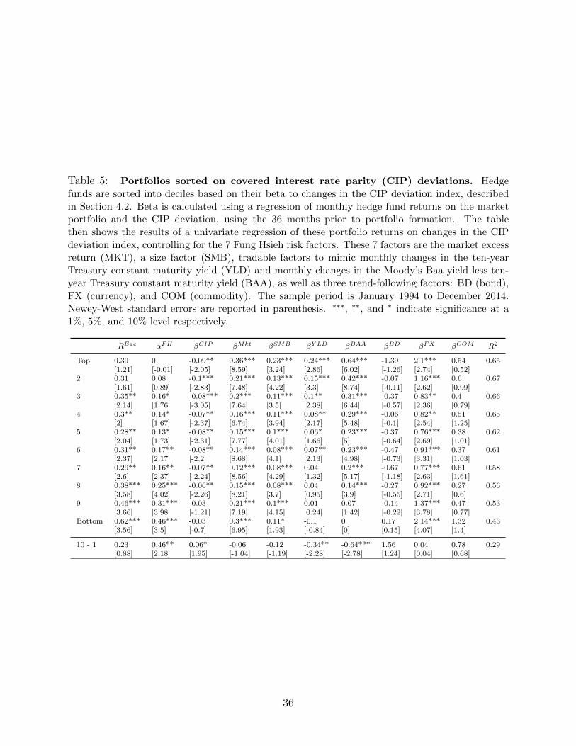
Table 5: Portfolios sorted on covered interest rate parity (CIP) deviations. Hedgefunds are sorted into deciles based on their beta to changes in the CIP deviation index, describedin Section 4.2. Beta is calculated using a regression of monthly hedge fund returns on the marketportfolio and the CIP deviation, using the 36 months prior to portfolio formation. The tablethen shows the results of a univariate regression of these portfolio returns on changes in the CIPdeviation index, controlling for the 7 Fung Hsieh risk factors. These 7 factors are the market excessreturn (MKT), a size factor (SMB), tradable factors to mimic monthly changes in the ten-yearTreasury constant maturity yield (YLD) and monthly changes in the Moody’s Baa yield less ten-year Treasury constant maturity yield (BAA), as well as three trend-following factors: BD (bond),FX (currency), and COM (commodity). The sample period is January 1994 to December 2014.Newey-West standard errors are reported in parenthesis. ∗∗∗, ∗∗, and ∗ indicate significance at a1%, 5%, and 10% level respectively.

RExc αFH βCIP βMkt βSMB βY LD βBAA βBD βFX βCOM R2

Top 0.39 0 -0.09** 0.36*** 0.23*** 0.24*** 0.64*** -1.39 2.1*** 0.54 0.65[1.21] [-0.01] [-2.05] [8.59] [3.24] [2.86] [6.02] [-1.26] [2.74] [0.52]

2 0.31 0.08 -0.1*** 0.21*** 0.13*** 0.15*** 0.42*** -0.07 1.16*** 0.6 0.67[1.61] [0.89] [-2.83] [7.48] [4.22] [3.3] [8.74] [-0.11] [2.62] [0.99]

3 0.35** 0.16* -0.08*** 0.2*** 0.11*** 0.1** 0.31*** -0.37 0.83** 0.4 0.66[2.14] [1.76] [-3.05] [7.64] [3.5] [2.38] [6.44] [-0.57] [2.36] [0.79]

4 0.3** 0.14* -0.07** 0.16*** 0.11*** 0.08** 0.29*** -0.06 0.82** 0.51 0.65[2] [1.67] [-2.37] [6.74] [3.94] [2.17] [5.48] [-0.1] [2.54] [1.25]

5 0.28** 0.13* -0.08** 0.15*** 0.1*** 0.06* 0.23*** -0.37 0.76*** 0.38 0.62[2.04] [1.73] [-2.31] [7.77] [4.01] [1.66] [5] [-0.64] [2.69] [1.01]

6 0.31** 0.17** -0.08** 0.14*** 0.08*** 0.07** 0.23*** -0.47 0.91*** 0.37 0.61[2.37] [2.17] [-2.2] [8.68] [4.1] [2.13] [4.98] [-0.73] [3.31] [1.03]

7 0.29** 0.16** -0.07** 0.12*** 0.08*** 0.04 0.2*** -0.67 0.77*** 0.61 0.58[2.6] [2.37] [-2.24] [8.56] [4.29] [1.32] [5.17] [-1.18] [2.63] [1.61]

8 0.38*** 0.25*** -0.06** 0.15*** 0.08*** 0.04 0.14*** -0.27 0.92*** 0.27 0.56[3.58] [4.02] [-2.26] [8.21] [3.7] [0.95] [3.9] [-0.55] [2.71] [0.6]

9 0.46*** 0.31*** -0.03 0.21*** 0.1*** 0.01 0.07 -0.14 1.37*** 0.47 0.53[3.66] [3.98] [-1.21] [7.19] [4.15] [0.24] [1.42] [-0.22] [3.78] [0.77]

Bottom 0.62*** 0.46*** -0.03 0.3*** 0.11* -0.1 0 0.17 2.14*** 1.32 0.43[3.56] [3.5] [-0.7] [6.95] [1.93] [-0.84] [0] [0.15] [4.07] [1.4]

10 - 1 0.23 0.46** 0.06* -0.06 -0.12 -0.34** -0.64*** 1.56 0.04 0.78 0.29[0.88] [2.18] [1.95] [-1.04] [-1.19] [-2.28] [-2.78] [1.24] [0.04] [0.68]

36

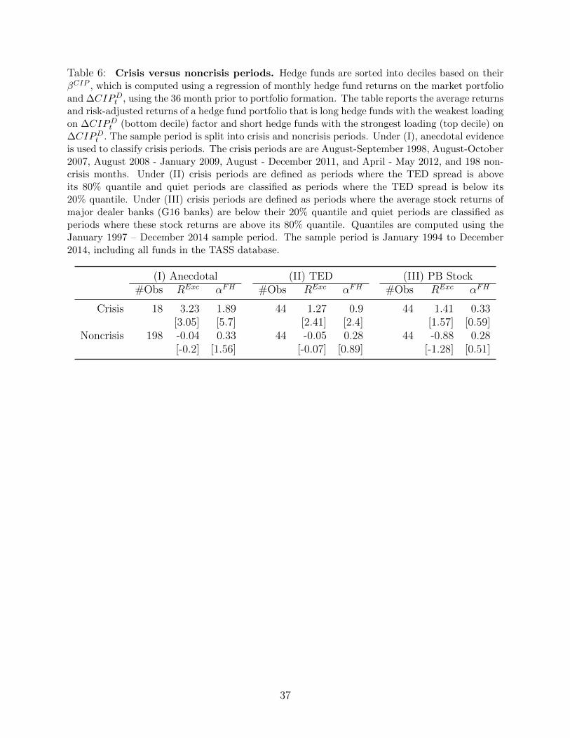
Table 6: Crisis versus noncrisis periods. Hedge funds are sorted into deciles based on theirβCIP , which is computed using a regression of monthly hedge fund returns on the market portfolioand ∆CIPDt , using the 36 month prior to portfolio formation. The table reports the average returnsand risk-adjusted returns of a hedge fund portfolio that is long hedge funds with the weakest loadingon ∆CIPDt (bottom decile) factor and short hedge funds with the strongest loading (top decile) on∆CIPDt . The sample period is split into crisis and noncrisis periods. Under (I), anecdotal evidenceis used to classify crisis periods. The crisis periods are are August-September 1998, August-October2007, August 2008 - January 2009, August - December 2011, and April - May 2012, and 198 non-crisis months. Under (II) crisis periods are defined as periods where the TED spread is aboveits 80% quantile and quiet periods are classified as periods where the TED spread is below its20% quantile. Under (III) crisis periods are defined as periods where the average stock returns ofmajor dealer banks (G16 banks) are below their 20% quantile and quiet periods are classified asperiods where these stock returns are above its 80% quantile. Quantiles are computed using theJanuary 1997 – December 2014 sample period. The sample period is January 1994 to December2014, including all funds in the TASS database.

(I) Anecdotal (II) TED (III) PB Stock#Obs RExc αFH #Obs RExc αFH #Obs RExc αFH

Crisis 18 3.23 1.89 44 1.27 0.9 44 1.41 0.33[3.05] [5.7] [2.41] [2.4] [1.57] [0.59]

Noncrisis 198 -0.04 0.33 44 -0.05 0.28 44 -0.88 0.28[-0.2] [1.56] [-0.07] [0.89] [-1.28] [0.51]

37

Table 7: Characteristics of the CIP-deviation-sorted hedge fund portfolios. This tablereports the average characteristics and average allocations within hedge fund style for the 10 CIP-beta-sorted portfolios from Table 5. See Table 1 for a description of the different variables.

Portfolio Rank Top 2 3 4 5 6 7 8 9 Bottom

Panel A: Characteristics

Backfilled 0.28 0.33 0.35 0.36 0.36 0.36 0.34 0.33 0.31 0.32USD 0.83 0.81 0.78 0.74 0.73 0.72 0.73 0.77 0.79 0.83X 0.83 0.90 0.93 0.94 0.94 0.95 0.95 0.94 0.92 0.86AUM 199.61 223.93 254.67 251.29 236.76 219.31 217.91 205.33 175.23 164.07LockUpPeriod 3.06 2.97 2.63 2.46 2.37 2.22 2.46 2.71 2.98 3.14RedemptionNoticePeriod 31.94 34.78 36.88 38.64 39.88 38.54 38.56 37.52 33.80 30.25MinimumInvestment 1.02 1.35 1.35 7.59 12.05 5.81 4.36 2.21 2.60 2.32ManagementFee 1.51 1.47 1.43 1.39 1.37 1.36 1.35 1.36 1.41 1.50IncentiveFee 16.09 14.94 12.98 13.36 13.52 13.33 14.57 15.87 16.85 17.55HighWaterMark 0.59 0.55 0.54 0.52 0.47 0.50 0.50 0.50 0.56 0.60Leveraged 0.66 0.58 0.52 0.51 0.48 0.48 0.49 0.52 0.57 0.64PersonalCapital 0.39 0.34 0.30 0.28 0.27 0.27 0.28 0.31 0.35 0.37Age 85.92 89.25 90.34 87.63 87.22 87.58 87.70 87.27 87.54 87.83

Panel B: Allocation within hedge fund style (%)

Convertible Arbitrage 2.15 2.89 3.47 2.81 2.70 3.16 3.32 2.72 1.44 1.23Fund of Funds 11.52 26.68 42.34 49.76 53.60 52.78 46.05 35.24 21.42 11.51Long Short Equity 36.04 29.85 21.95 17.32 15.51 14.59 16.22 23.05 31.29 40.10Emerging Markets 14.32 8.29 5.06 3.49 2.81 2.46 2.79 3.92 5.89 9.14Equity Market Neutral 2.42 2.91 2.89 3.11 2.45 2.72 3.59 4.52 5.05 4.27Event Driven 4.24 5.83 7.01 7.61 8.59 9.01 10.39 11.34 10.25 5.29Global Macro 5.57 3.38 2.48 1.79 1.45 1.48 1.58 2.44 3.42 4.78Fixed Income Arbitrage 3.94 3.29 2.57 2.87 2.49 2.72 3.10 2.61 2.96 1.60Multi Strategy 5.67 6.39 5.11 5.47 4.81 4.97 5.82 6.41 5.27 3.67Managed Futures 10.65 6.87 4.12 3.37 3.47 3.57 4.06 5.22 8.89 15.48Other 3.48 3.63 2.99 2.41 2.12 2.54 3.09 2.54 4.12 2.93

38

Table 8: Robustness checks using cross-sectional regressions. Fama and MacBeth (1973)regressions of the cross section of monthly hedge fund alphas (relative to the Fung-Hsieh 7 factormodel). In the first and second regression, alphas are computed using all returns reported in thedatabase. Under Backfill, I repeat the analysis dropping backfilled return observations. Underunsmoothed, I use the procedure by Getmansky et al. (2004) to un-smooth hedge fund returnsbefore repeating the analysis. Under Survivorship, I replace the last alpha with −20% beforerepeating the analysis. Newey-West standard errors are reported in parenthesis. ∗∗∗, ∗∗, and ∗

indicate significance at a 1%, 5%, and 10% level respectively.

CIP Redemption Redemption Lockup StyleIntercept beta Age Size Frequency Notice Period Dummies

No Controls 0.49*** 4.103**[3.89] [2.34]

Controls 0.238 4.202** -0.071** 0.06*** -0.001 0.043** 0.008*** Yes[1.64] [2.46] [-2.01] [5.28] [-0.2] [2.52] [3.44]

Backfill -0.03 3.821** -0.075* 0.088*** -0.002 0.064*** 0.009*** Yes[-0.2] [2.06] [-1.86] [6.38] [-0.37] [3] [3.02]

Unsmoothed 0.26* 2.516** -0.106*** 0.054*** 0 0.023 0.008*** Yes[1.86] [2.38] [-2.72] [3.84] [-0.09] [1.41] [3.41]

Survivorship -0.263 4.714** -0.046 0.114*** -0.007 0.044** 0.009*** Yes[-1.24] [1.99] [-1.14] [6.94] [-1.51] [2.18] [3.11]

39