Risk Containmentfor Hedge Funds

Anish R. Shah, CFANorthfield Information Services

Anish@northinfo.com

High Net Worth SeminarNaples, FL

Jan 24, 2008

Investment Vehicle that Experienced Explosive Growth

• 30 fold growth in assets under management since 1990

• estimate > 2000 new funds launched in 2006• in US equities: 5% of assets, but 30% of

trading volume(source: sec.gov)

• Premium for top funds, e.g. Caxton 3/30, Renaissance 5/44, SAC 50% of profits

Extensive Literature• Weisman, A. “Informationless Investing And Hedge Fund Performance

Measurement Bias,” Journal of Portfolio Management, 2002, v28(4,Summer), 80-91.

• Lo, A. “Risk Management for Hedge Funds: Introduction and Overview,”Financial Analysts Journal, 2001, v57(6,Nov/Dec), 16–33.

• Bondarenko, O. “Market Price of Variance Risk and Performance of Hedge Funds,” SSRN working paper, Mar 2004.

• Getmansky, M. et al. “An econometric model of serial correlation and illiquidity in hedge fund returns,” Journal of Financial Economics, 2004, v74(3,Dec), 529-609.

• Jorion, P. “Risk management lessons from Long-Term Capital Management,” European Financial Management, 2000, v6(3), 277-300.

• Chow, G. & Kritzman, M. “Value at Risk for Portfolios with Short Positions,”Journal of Portfolio Management, 2002 v28(3,Spring), 73-81.

• Winston, K. “Long/short portfolio behavior with barriers,” Northfield Research Conference, 2006.

• Carmona, R. & Durrleman, V. “Pricing and Hedging Spread Options,” SIAM Review, 2003, v45(4), 627-685.

Fundamental Idea• For both investors and managers, hedge

funds (though they may be benchmarked to long-only or cash) are a totally different animal

• Non-Gaussian return distributions• Liquidity and leverage/credit

considerations• Dynamic investment strategies

• Traditional measures of performance and risk – std dev, tracking error, β, α, Sharpe ratio – are non-descriptive

Part I: Complications for the Investor

• Lo 2001, “Risk Management for Hedge Funds: Introduction and Overview”

Weisman 2002, “Informationless Investing And Hedge Fund Performance Measurement Bias”

• How to manufacture performance with no skill

1. No Skill α

From Lo 2001:

The Secret: Short Volatility(sell insurance - risk is invisible until it

happens)• Writing options

Lo’s example sells out of the money puts

• Writing synthetic options by ∆ hedging (dynamically altering the mix of stock and cash)Executed without owning derivatives

• Issuing credit default swaps

• Betting that spreads return to typical levelse.g. LTCM, see Jorion 2000

Frequent Small Gains Exchanged for Infrequent Large Losses

Performance of Short VolStrategy

From Weisman 2002:

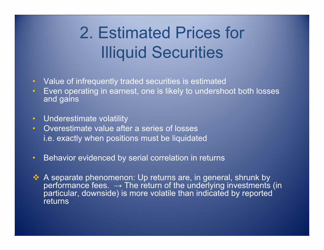
2. Estimated Prices forIlliquid Securities

• Value of infrequently traded securities is estimated• Even operating in earnest, one is likely to undershoot both losses

and gains

• Underestimate volatility• Overestimate value after a series of losses

i.e. exactly when positions must be liquidated

• Behavior evidenced by serial correlation in returns

A separate phenomenon: Up returns are, in general, shrunk by performance fees. → The return of the underlying investments (in particular, downside) is more volatile than indicated by reported returns

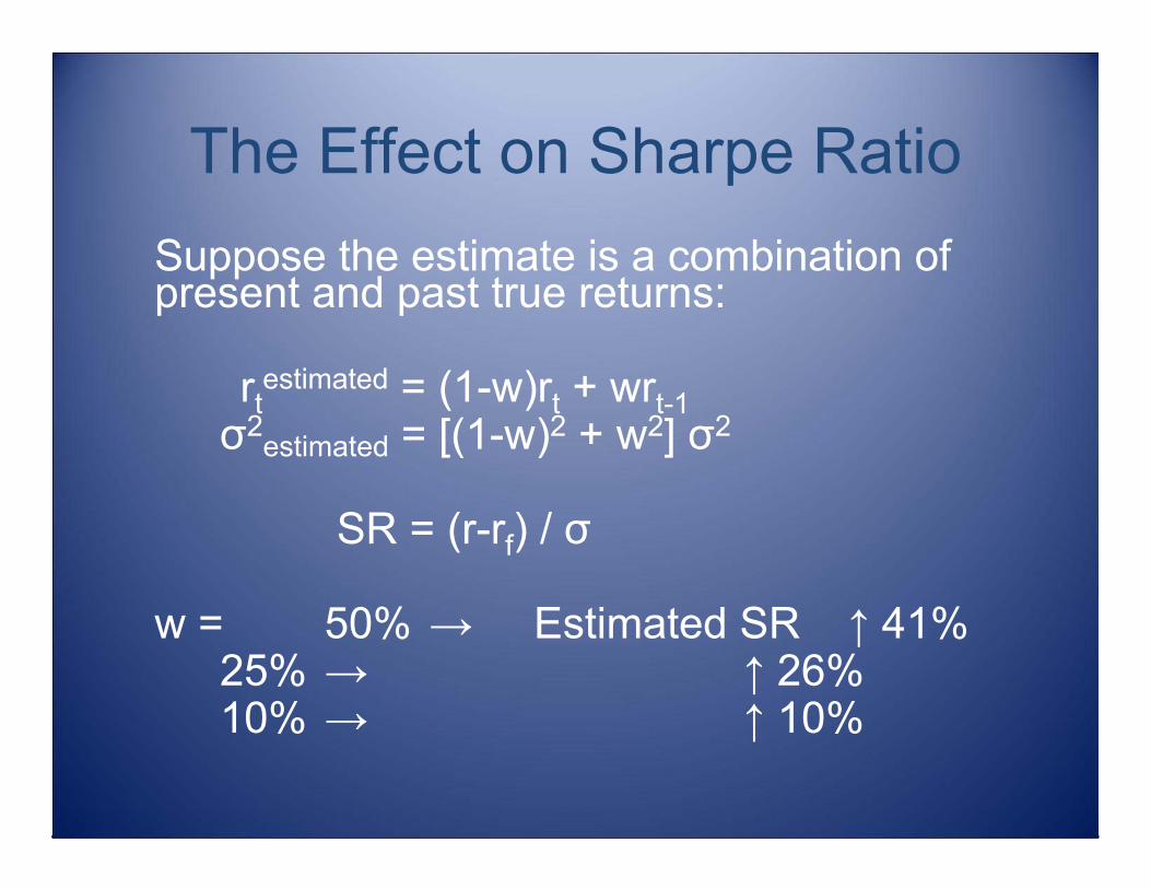
The Effect on Sharpe RatioSuppose the estimate is a combination of present and past true returns:

rtestimated = (1-w)rt + wrt-1

σ2estimated = [(1-w)2 + w2] σ2

SR = (r-rf) / σ

w = 50% → Estimated SR ↑ 41%25% → ↑ 26%10% → ↑ 10%

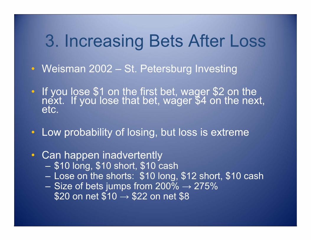
3. Increasing Bets After Loss• Weisman 2002 – St. Petersburg Investing

• If you lose $1 on the first bet, wager $2 on the next. If you lose that bet, wager $4 on the next, etc.

• Low probability of losing, but loss is extreme

• Can happen inadvertently– $10 long, $10 short, $10 cash– Lose on the shorts: $10 long, $12 short, $10 cash– Size of bets jumps from 200% → 275%

$20 on net $10 → $22 on net $8

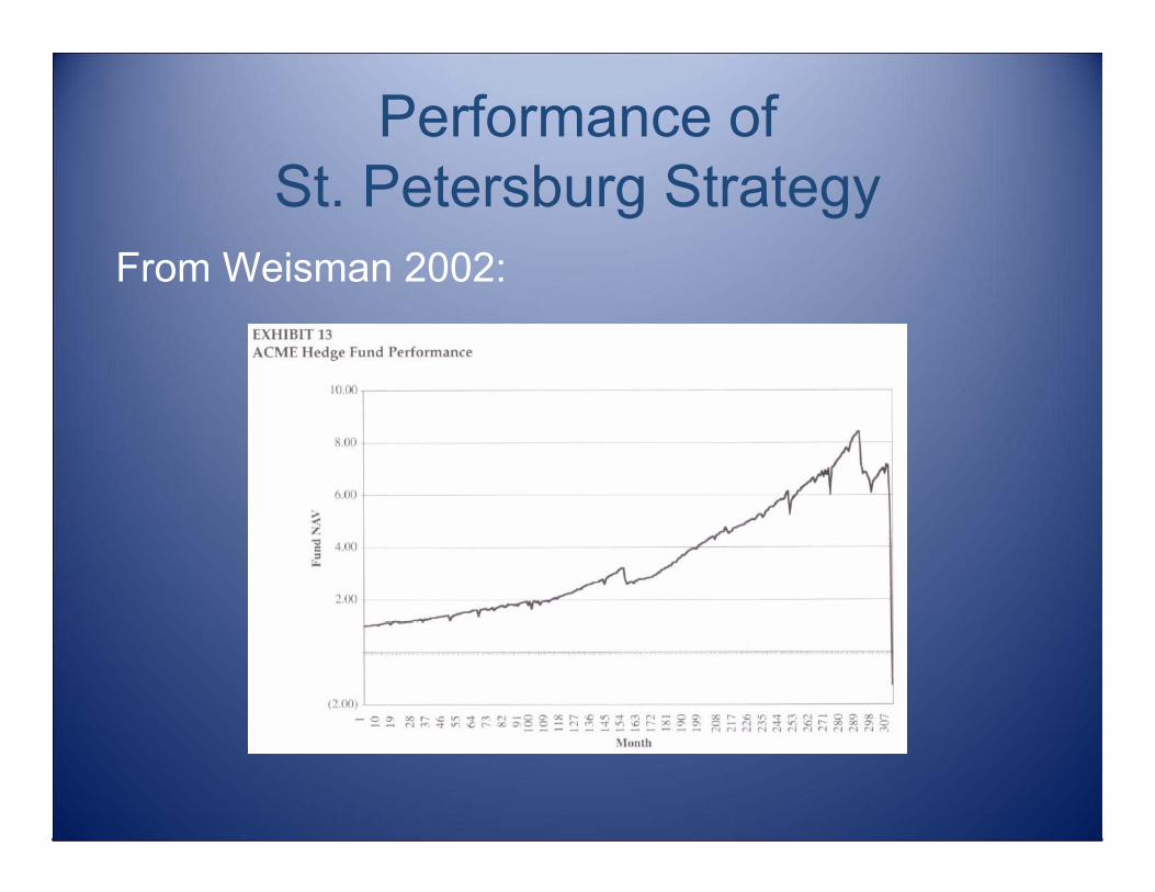
Performance ofSt. Petersburg Strategy

From Weisman 2002:

Theory Meets Reality• LTCM

90% of return explained by monthly changes in credit spread1/98 → 8/98, lost 52% of its value. Leverage jumped from 28:1 ↑ 55:1

• Nick Maounis, founder of Amaranth Advisors:"In September, 2006, a series of unusual and unpredictable market events caused the fund's natural-gas positions, including spreads, to incur dramatic losses”

“We had not expected that we would be faced with a market that would move so aggressively against our positions without the market offering any ability to liquidate positions economically.”

"We viewed the probability of market movements such as those that took place in September as highly remote … But sometimes, even the highly improbable happens.”

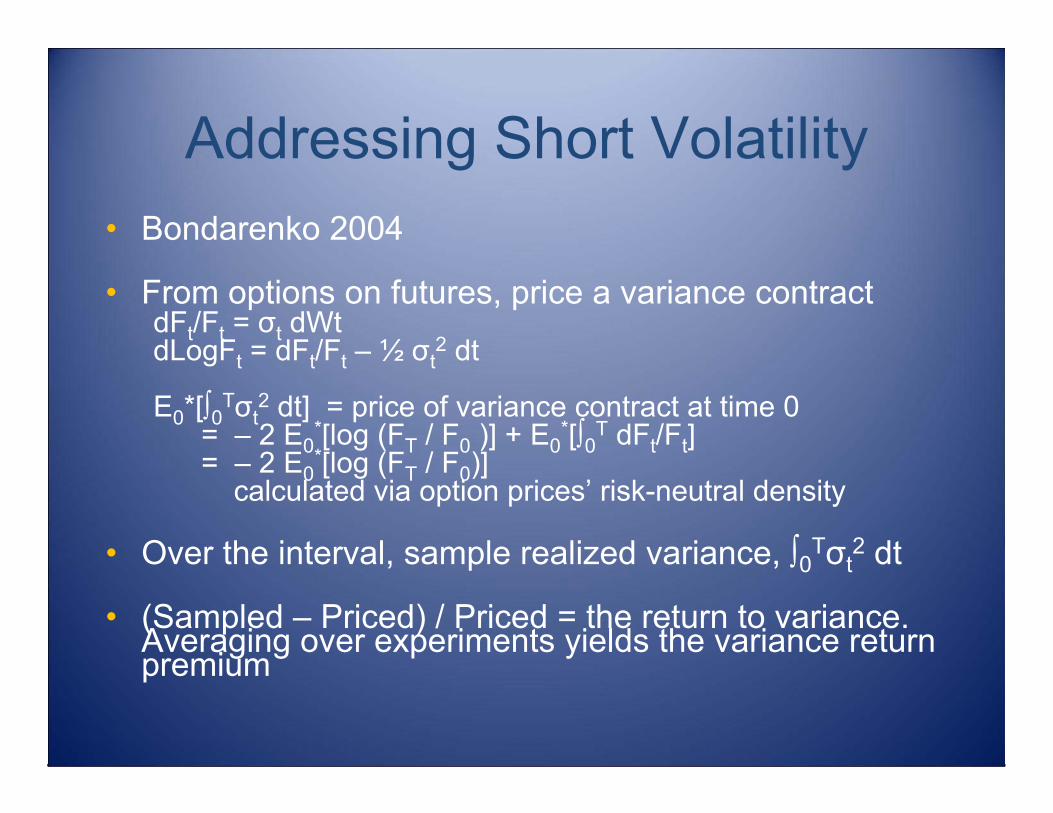
Addressing Short Volatility• Bondarenko 2004

• From options on futures, price a variance contractdFt/Ft = σt dWtdLogFt = dFt/Ft – ½ σt

2 dt

E0*[∫0Tσt2 dt] = price of variance contract at time 0

= – 2 E0*[log (FT / F0 )] + E0

*[∫0T dFt/Ft]= – 2 E0

*[log (FT / F0)]calculated via option prices’ risk-neutral density

• Over the interval, sample realized variance, ∫0Tσt2 dt

• (Sampled – Priced) / Priced = the return to variance. Averaging over experiments yields the variance return premium

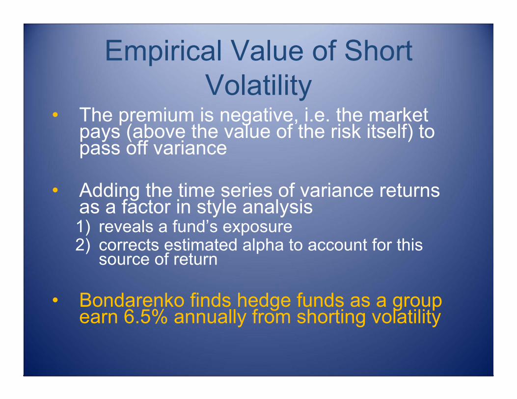
Empirical Value of Short Volatility

• The premium is negative, i.e. the market pays (above the value of the risk itself) to pass off variance

• Adding the time series of variance returns as a factor in style analysis1) reveals a fund’s exposure2) corrects estimated alpha to account for this

source of return

• Bondarenko finds hedge funds as a group earn 6.5% annually from shorting volatility

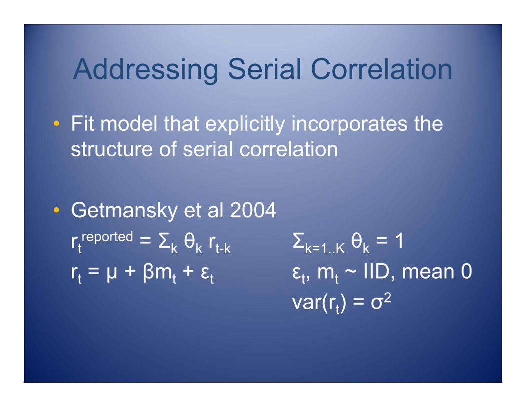
Addressing Serial Correlation

• Fit model that explicitly incorporates the structure of serial correlation

• Getmansky et al 2004rt

reported = Σk θk rt-k Σk=1..K θk = 1rt = µ + βmt + εt εt, mt ~ IID, mean 0

var(rt) = σ2

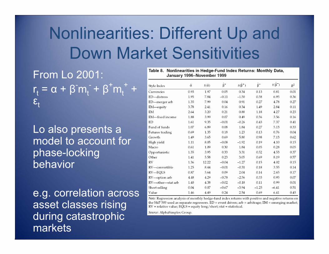
Nonlinearities: Different Up and Down Market Sensitivities

From Lo 2001:rt = α + β-mt

- + β+mt+ +

εt

Lo also presents a model to account for phase-locking behavior

e.g. correlation across asset classes rising during catastrophic markets

Part II: Complications for the Manager

• Liquidity• Stability• Limited Liability

– Chow & Kritzman 2002, “Value at Risk for Portfolios with Short Positions”

– Winston 2006, “Long/short portfolio behavior with barriers”

1. Liquidity Risk• An example: big drops in Aug 2007

8/3 SP500 ↓ 2.7%, R2000 ↓ 3.6%8/6-8 SP500 ↑ 4.5%, R2000 ↑ 5.3%

8/9 SP500 ↓ 3.0%, R2000 ↓ 1.4%8/10 SP500 ↑ 0.0%, R2000 ↑ 0.5%

8/13-15 SP500 ↓ 3.2%, R2000 ↓ 4.7%8/16-17 SP500 ↑ 2.8%, R2000 ↑ 4.5%,

8/27-28 SP500 ↓ 3.2%, R2000 ↓ 3.9%8/29 SP500 ↑ 2.2%, R2000 ↑ 2.5%

• Over the month, SP500 up 1.3%, R2000 up 2.2%

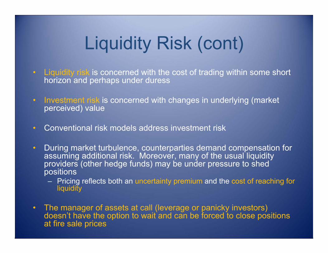
Liquidity Risk (cont)• Liquidity risk is concerned with the cost of trading within some short

horizon and perhaps under duress

• Investment risk is concerned with changes in underlying (market perceived) value

• Conventional risk models address investment risk

• During market turbulence, counterparties demand compensation forassuming additional risk. Moreover, many of the usual liquidityproviders (other hedge funds) may be under pressure to shed positions– Pricing reflects both an uncertainty premium and the cost of reaching for

liquidity

• The manager of assets at call (leverage or panicky investors) doesn’t have the option to wait and can be forced to close positions at fire sale prices

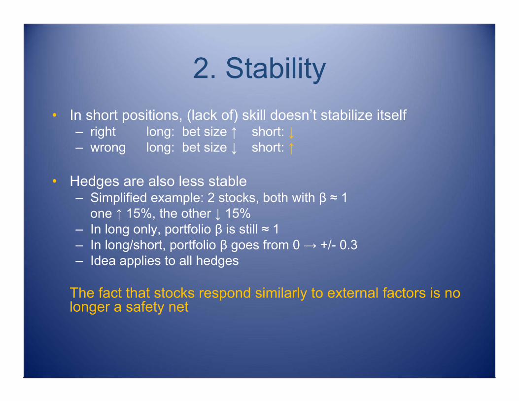
2. Stability• In short positions, (lack of) skill doesn’t stabilize itself

– right long: bet size ↑ short: ↓– wrong long: bet size ↓ short: ↑

• Hedges are also less stable– Simplified example: 2 stocks, both with β ≈ 1

one ↑ 15%, the other ↓ 15%– In long only, portfolio β is still ≈ 1– In long/short, portfolio β goes from 0 → +/- 0.3– Idea applies to all hedges

The fact that stocks respond similarly to external factors is nolonger a safety net

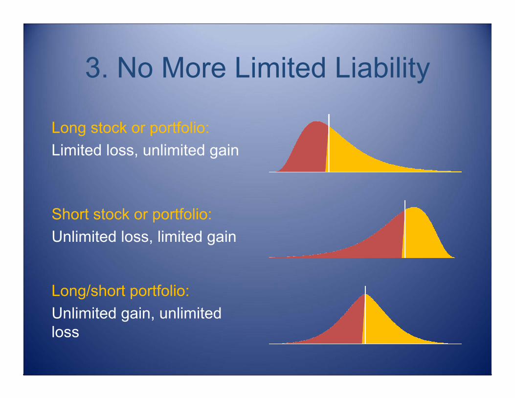
3. No More Limited Liability

Long stock or portfolio:Limited loss, unlimited gain

Short stock or portfolio:Unlimited loss, limited gain

Long/short portfolio:Unlimited gain, unlimited loss

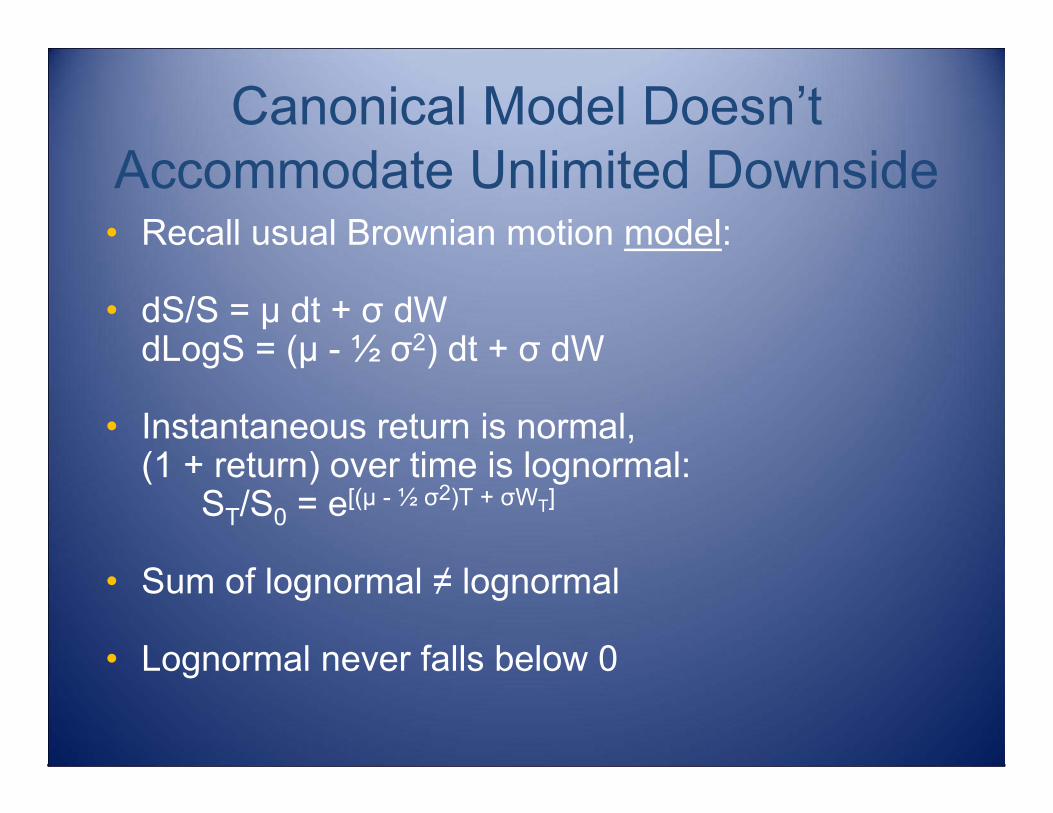
Canonical Model Doesn’t Accommodate Unlimited Downside• Recall usual Brownian motion model:

• dS/S = µ dt + σ dWdLogS = (µ - ½ σ2) dt + σ dW

• Instantaneous return is normal,(1 + return) over time is lognormal:

ST/S0 = e[(µ - ½ σ2)T + σWT]

• Sum of lognormal ≠ lognormal

• Lognormal never falls below 0

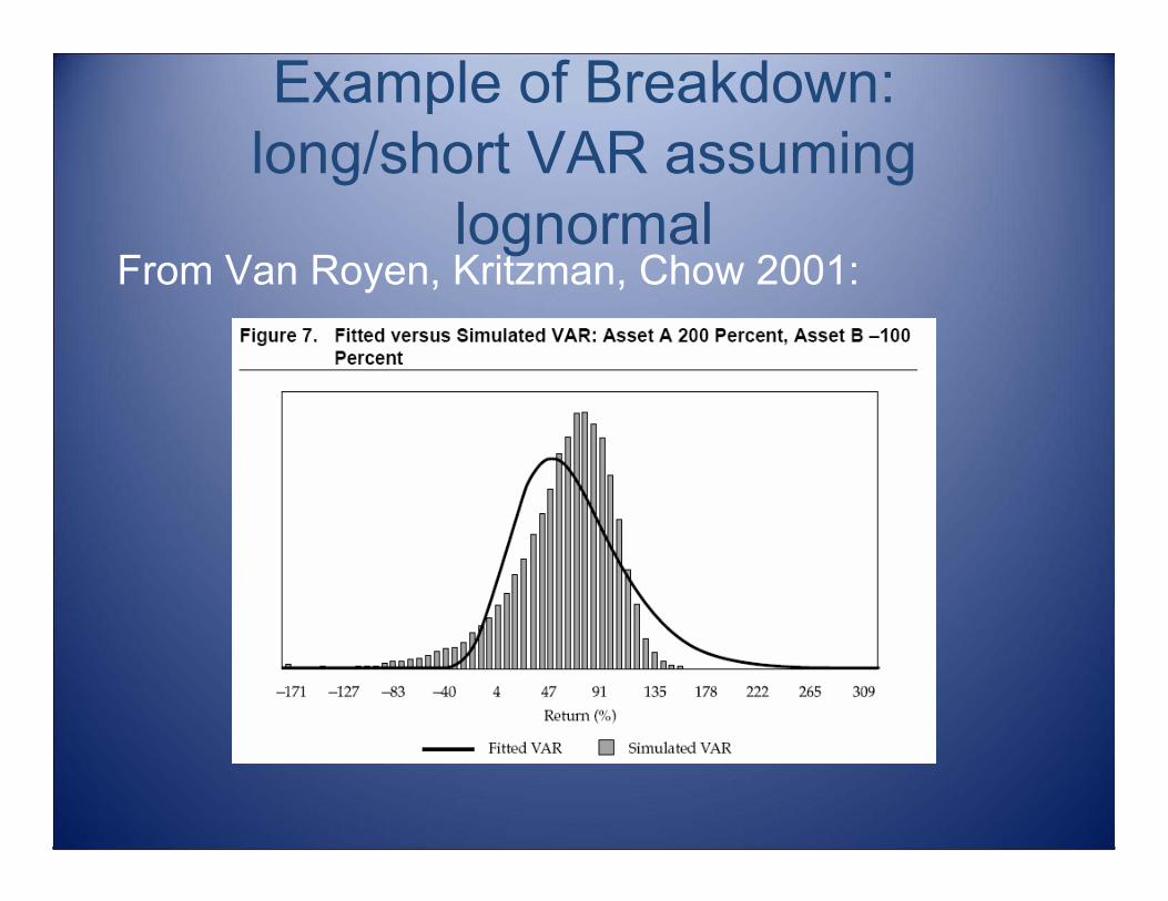
Example of Breakdown:long/short VAR assuming

lognormal From Van Royen, Kritzman, Chow 2001:

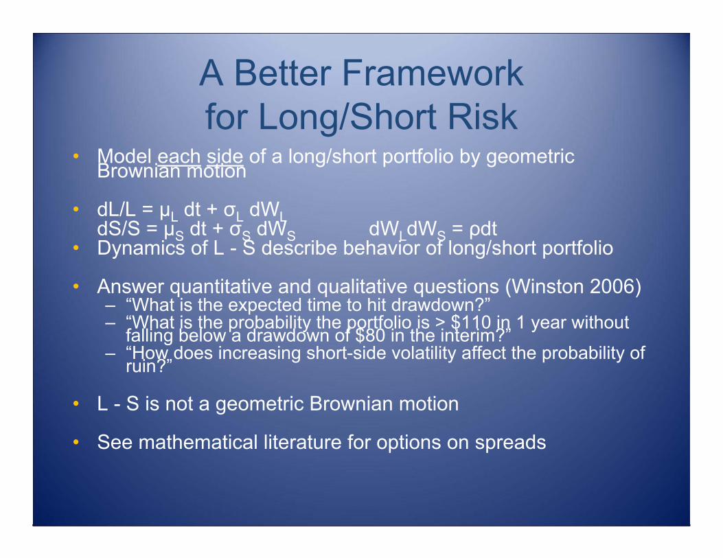
A Better Frameworkfor Long/Short Risk

• Model each side of a long/short portfolio by geometric Brownian motion

• dL/L = µL dt + σL dWLdS/S = µS dt + σS dWS dWLdWS = ρdt

• Dynamics of L - S describe behavior of long/short portfolio

• Answer quantitative and qualitative questions (Winston 2006)– “What is the expected time to hit drawdown?”– “What is the probability the portfolio is > $110 in 1 year without

falling below a drawdown of $80 in the interim?”– “How does increasing short-side volatility affect the probability of

ruin?”

• L - S is not a geometric Brownian motion

• See mathematical literature for options on spreads

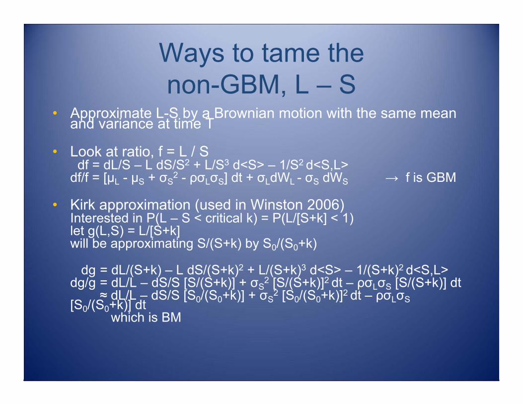
Ways to tame thenon-GBM, L – S

• Approximate L-S by a Brownian motion with the same mean and variance at time T

• Look at ratio, f = L / Sdf = dL/S – L dS/S2 + L/S3 d<S> – 1/S2 d<S,L>

df/f = [µL - µS + σS2 - ρσLσS] dt + σLdWL - σS dWS → f is GBM

• Kirk approximation (used in Winston 2006)Interested in P(L – S < critical k) = P(L/[S+k] < 1) let g(L,S) = L/[S+k]will be approximating S/(S+k) by S0/(S0+k)

dg = dL/(S+k) – L dS/(S+k)2 + L/(S+k)3 d<S> – 1/(S+k)2 d<S,L>dg/g = dL/L – dS/S [S/(S+k)] + σS

2 [S/(S+k)]2 dt – ρσLσS [S/(S+k)] dt≈ dL/L – dS/S [S0/(S0+k)] + σS

2 [S0/(S0+k)]2 dt – ρσLσS[S0/(S0+k)] dtwhich is BM

An Application of the ModelSuccess and failure surfacesfrom Winston 2006:

Summary• Hedge funds offer investment strategies

poorly described by traditional tools and measures.

• If investors aren’t aware of the hidden risks, surely they will select for them.e.g. 4:00 mile is fast, 3:30 mile = a goat?

• Managers of long/short portfolios are exposed to phenomena not present in long-only. Avoiding a blow-up requires extra vigilance.