heat transfer lab manual - mrcet.com iii-ii.pdf · 1 heat transfer through composite wall 03-08 2...
TRANSCRIPT
HEAT TRANSFER LAB 2016
DEPARTMENT OF MECHANICAL ENGINEERING (MRCET) Page 1
HEAT TRANSFER LAB MANUAL
Department of Mechanical Engineering
MallaReddy College of Engineering and Technology
Maisammaguda, Dhulapally, Secunderabad-14
HEAT TRANSFER LAB 2016
DEPARTMENT OF MECHANICAL ENGINEERING (MRCET) Page 2
INDEX
S.NO. NAME OF THE EXPERIMENT PAGE NOs.
1 HEAT TRANSFER THROUGH COMPOSITE WALL 03-08
2 CRITICAL HEAT FLUX APPARATUS 09-12
3 MEASUREMENT OF SURFACE EMMISSIVITY 13-18
4 HEAT TRANSFER THROUGH FORCED CONVECTION 19-25
5 HEAT PIPE DEMONSTRATION 26-27
6 HEAT TRANSFER THROUGH LAGGED PIPE 28-31
7 HEAT TRANSFER THROUGH NATURAL CONVECTION 32-38
8 PARALLEL & COUNTER FLOW HEAT EXCHANGER 39-45
9 HEAT TRANSFER THROUTH PIN-FIN 46-49
10 STEFAN BOLTZMAN’S APPARATUS 51-54
11 THERMAL CONDUCTIVITY OF CONCENTRIC SPHERE 55-58
12 THERMAL CONDUCTIVITY OF METAL ROD 59-63
13 TRANSIENT HEAT CONDUCTION APPARATUS 64-70
14 CONDENSATION APPARATUS 71-83
HEAT TRANSFER LAB 2016
DEPARTMENT OF MECHANICAL ENGINEERING (MRCET) Page 3
1.HEAT TRANSFER THROUGH COMPOSITE WALL
INTRODUCTION:
In engineering applications, we deal with many problems. Heat Transfer through composite
walls is one of them. It is the transport of energy between two or more bodies of different thermal
conductivity arranged in series or parallel. For example, a fastener joining two mediums also acts as
one of the layers between these mediums. Hence, the thermal conductivity of the fastener is also
very much necessary in determining the overall heat transfer through the medium. An attempt has
been made to show the concept of heat transfers through composite walls.
DESCRIPTION OF THE APPARATUS:
The apparatus consists of three slabs of Mild Steel, Bakelite and Aluminum materials of
thickness 25, 20 & 12mm respectively clamped in the center using screw rod.
At the center of the composite wall a heater is fitted. End losses from the composite wall
are minimized by providing thick insulation all round to ensure unidirectional heat flow.
Front transparent acrylic enclosure to minimize the disturbances of the surrounding and
also for safety of the composite slab when not in use.
Control panel instrumentation consists of:
a. Mains on indicatorb. Console On switch for activation of the control panel.c. Scanner for measurement of
i. Temperatures at various locations of the slab.ii. Input Voltage.iii. Input Current.
d. Heater regulator to regulate the input voltage.With this the whole arrangement is mounted on an aesthetically designed self-sustained
Nova pone control panel.
AIM: To determine
1. The overall thermal conductance (C) for a composite wall and to compare with theoretical
value.
2. Temperature distribution across the width of the composite wall.
HEAT TRANSFER LAB 2016
DEPARTMENT OF MECHANICAL ENGINEERING (MRCET) Page 4
PROCEDURE : MANUAL
1. Symmetrically arrange the plates and ensure perfect contact between the plates.
2. Give necessary electrical connections to the instruments.
3. Switch ON mains and the CONSOLE.
4. Set the heater regulator to the known value.
5. Wait for sufficient time to allow temperature to reach steady values.
6. Note down the Temperatures, voltage and current using the Data logger.
7. Calculate the overall conductance using the formulae given below.
8. Repeat the experiment for different heat input.
OBSERVATIONS:
Sl. No.
Temperatures ∞C
Heater
Input
T1 T2 T3 T4 T5 T6 V I
1
2
3
4
5
PROCEDURE: COMPUTERIZED
READINGS – COMPUTERIZED
1. Symmetrically arrange the plates and ensure perfect contact between the plates.
2. Give necessary electrical connections to the instruments.
3. Switch ON mains and the CONSOLE.
4. Set the heater regulator to the known value.
5. Wait for sufficient time to allow temperature to reach steady values.
6. Turn on the computer switch on the panel.
7. Switch on the computer.
HEAT TRANSFER LAB 2016
DEPARTMENT OF MECHANICAL ENGINEERING (MRCET) Page 5
8. Open the “ HEAT TRANSFER Software” from the installed location a welcome screen will be
displayed
9. Follow the below steps to operate through software
a. Login using the given password into the software
b. Screen will display the concept of the equipment. Now login to the experiment by
clicking the “Click to login” button on the screen.
c. Give required username for the experiment to be conducted.
d. Once the software is opened, the main screen will be displaced
e. Now, press “START” button, and the small screen will opened for any messages and
also Specifications to be entered.
f. Enter the parameters listed for particular test under study.
g. Now, set the heater regulator to known valve.
h. Wait for sufficient time to allow temperature to reach steady values.
i. The software starts displaying the calculated values which can be cross verified based on the formulae give after.
10. Click the “store” button to store, the value can be viewed anytime later.
11. After completion of the Experiment, press the “STOP” Button.
12. To view the stored data follow the procedure in Annexure.
CALCULATIONS ARE BASED ON THE BELOW FORMULAE:
1. HEAT FLUX ,
q = Watts
Where,
V = voltmeter reading, volts
I = ammeter reading, amps
A = Area of the plate/s = (pd2/4) m2, d = 0.2m
2. AVERAGE TEMPERATURES:
TA = T1
TB = (T2 + T3)/2
TC = (T4 + T5)/2
TD = T6
V x I
A
HEAT TRANSFER LAB 2016
DEPARTMENT OF MECHANICAL ENGINEERING (MRCET) Page 6
Where,
TA = Average inlet temperature to Aluminium.
TB = Average outlet temperature from Aluminimum.
Average inlet temperature of MS
TC = Average outlet temperature to MS.
Average inlet temperature to Bakelite.
TD = Average outlet temperature to Bakelite.
3. THERMAL CONDUCTANCE:
PRACTICAL:
W/m0 K
Where,
Q = heat input in watts
(TA – TD) = Temperature difference as calculated.
THEORETICAL:
1
C = W/m ∞K
1/A (L1 / K1 + L2 / K2 + L3 / K3)
K1 = 205 W/m ∞K
K2 = 25 W/m ∞K
K3 = 0.08 W/m ∞K
L1 = 12 mm L2 = 25 mm L3 = 20 mm
4. OVERALL THERMAL CONDUCTIVITY OF THE SLAB, K
W/m0K
Where, B = thickness of the plates on one side = 0.057m
HEAT TRANSFER LAB 2016
DEPARTMENT OF MECHANICAL ENGINEERING (MRCET) Page 7
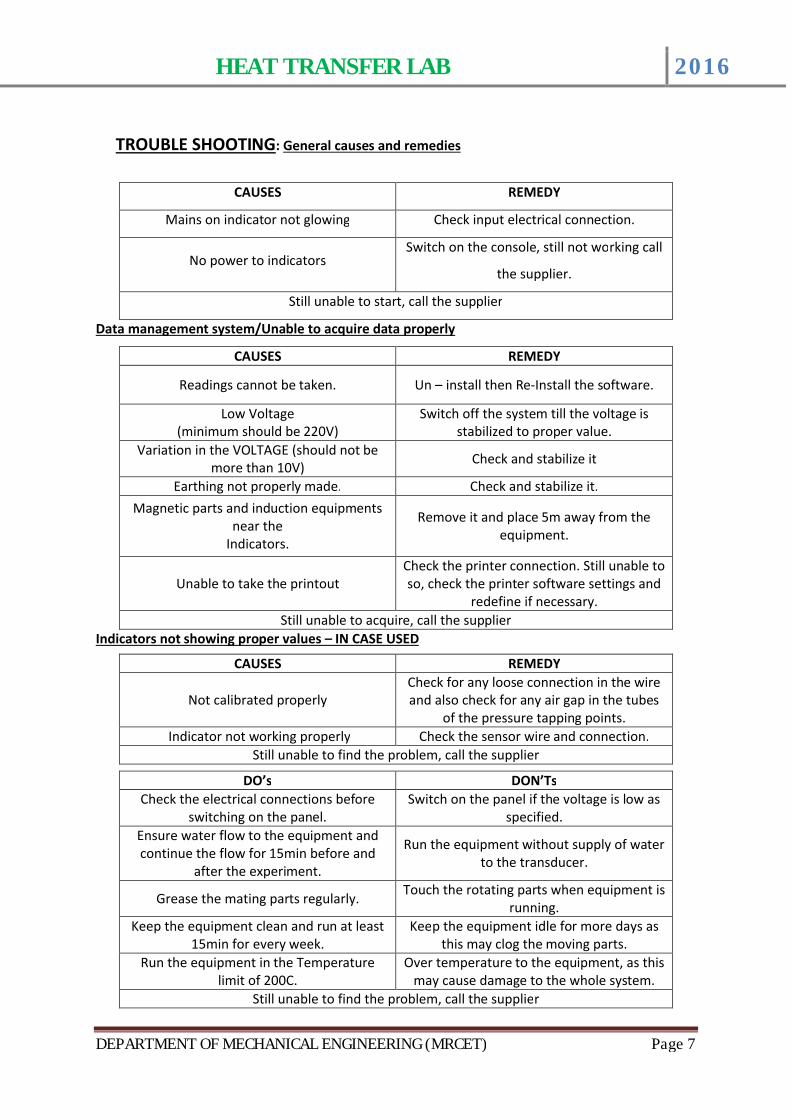
TROUBLE SHOOTING: General causes and remedies
CAUSES REMEDY
Mains on indicator not glowing Check input electrical connection.
No power to indicatorsSwitch on the console, still not working call
the supplier.
Still unable to start, call the supplier
Data management system/Unable to acquire data properly
CAUSES REMEDY
Readings cannot be taken. Un – install then Re-Install the software.
Low Voltage (minimum should be 220V)
Switch off the system till the voltage is stabilized to proper value.
Variation in the VOLTAGE (should not be more than 10V) Check and stabilize it
Earthing not properly made. Check and stabilize it.Magnetic parts and induction equipments
near the Indicators.
Remove it and place 5m away from the equipment.
Unable to take the printoutCheck the printer connection. Still unable to so, check the printer software settings and
redefine if necessary.Still unable to acquire, call the supplier
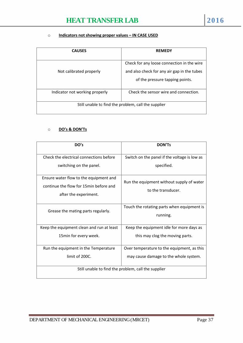
Indicators not showing proper values – IN CASE USED
CAUSES REMEDY
Not calibrated properlyCheck for any loose connection in the wire and also check for any air gap in the tubes
of the pressure tapping points.Indicator not working properly Check the sensor wire and connection.
Still unable to find the problem, call the supplier
DO’s DON’TsCheck the electrical connections before
switching on the panel.Switch on the panel if the voltage is low as
specified.Ensure water flow to the equipment and continue the flow for 15min before and
after the experiment.
Run the equipment without supply of water to the transducer.
Grease the mating parts regularly. Touch the rotating parts when equipment is running.
Keep the equipment clean and run at least 15min for every week.
Keep the equipment idle for more days as this may clog the moving parts.
Run the equipment in the Temperature limit of 200C.
Over temperature to the equipment, as this may cause damage to the whole system.
Still unable to find the problem, call the supplier
HEAT TRANSFER LAB 2016
DEPARTMENT OF MECHANICAL ENGINEERING (MRCET) Page 8
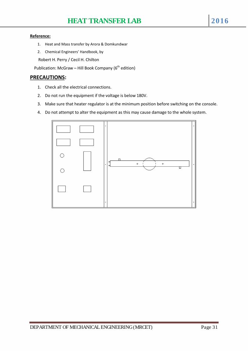
LIMITATIONS & PRECAUTIONS
1. Maximum Load is limited to 120V.
2. This is a general equipment for study in undergraduate level, for consideration of higher
level studies you can add any extra parameter required. For adding the parameters call the
supplier.
3. Don’t run the equipment if the voltage is less than 180V.
4. 230V, 1ph with neutral and proper earthing to be provided.
5. Don’t alter the equipment without the supervision of the supplier.
Reference:
1. Heat and Mass transfer by Arora & Domkundwar2. Chemical Engineers’ Handbook, by
Robert H. Perry / Cecil H. Chilton
Publication: McGraw – Hill Book Company (6th edition)
HEAT TRANSFER LAB 2016
DEPARTMENT OF MECHANICAL ENGINEERING (MRCET) Page 9
EXPT-2
CRITICAL HEAT FLUX APPARATUS1. INTRODUCTION:
Boiling and Condensation are the specific convection processes which is associated with
change of phase. The co – efficient of heat transfer are correspondingly very high when compared to
natural conventional process while the accompanying temperature difference are small (quite).
However, the visualization of this mode of heat transfer is more difficult and the actual
solutions are still difficult than conventional heat transfer process.
Commonly, this mode of heat transfer with change of phase is seen in Boilers, condensers in
power plants and evaporators in refrigeration system.
2. DESCRIPTION OF APPARATUS
1. The apparatus consists of a specially designed Glass Cylinder.
2. An arrangement above the Cylinder in the form of Bakelite plate is provided to place the
main Heater and the Nichrome wire heater arrangement.
3. The base is made of MS and is powder coated with Rubber cushion to place the Glass
cylinder.
4. Heater regulator to supply the regulated power input to the heater.
5. Digital Voltmeter and Ammeter to measure poser input ot the heater.
6. Thermocouples at suitable position to measure the temperatures of body and the
air.
7. Digital Temperature Indicator with channel selector to measure the temperatures.
8. The whole arrangement is mounted on an Aesthetically designed sturdy frame made of MS
tubes and NOVAPAN Board with all the provisions for holding the tanks and accessories.
AIM:1. To observe the formation of pool boiling and
2. To draw the graph of heat flux Vs. Bulk Temperature upto Burnout (Critical) condition.
HEAT TRANSFER LAB 2016
DEPARTMENT OF MECHANICAL ENGINEERING (MRCET) Page 10
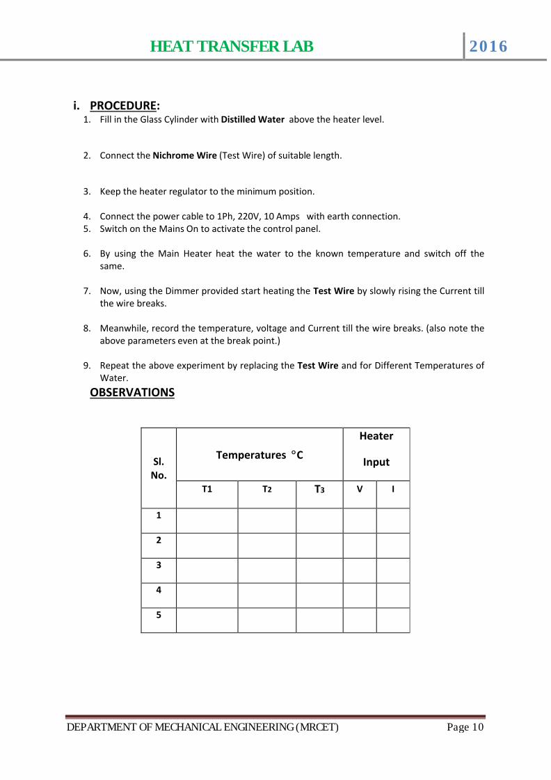
i. PROCEDURE:1. Fill in the Glass Cylinder with Distilled Water above the heater level.
2. Connect the Nichrome Wire (Test Wire) of suitable length.
3. Keep the heater regulator to the minimum position.
4. Connect the power cable to 1Ph, 220V, 10 Amps with earth connection.5. Switch on the Mains On to activate the control panel.
6. By using the Main Heater heat the water to the known temperature and switch off the same.
7. Now, using the Dimmer provided start heating the Test Wire by slowly rising the Current till the wire breaks.
8. Meanwhile, record the temperature, voltage and Current till the wire breaks. (also note the above parameters even at the break point.)
9. Repeat the above experiment by replacing the Test Wire and for Different Temperatures of Water.
OBSERVATIONS
Sl. No.
Temperatures ∞C
Heater
Input
T1 T2 T3 V I
1
2
3
4
5
HEAT TRANSFER LAB 2016
DEPARTMENT OF MECHANICAL ENGINEERING (MRCET) Page 11
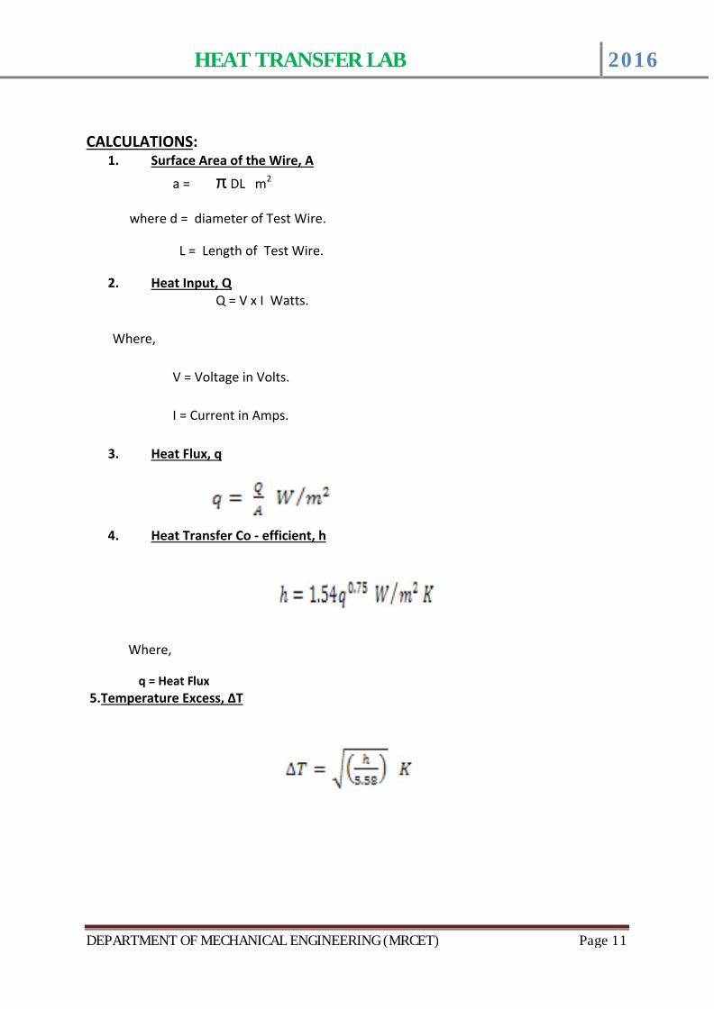
CALCULATIONS:1. Surface Area of the Wire, A
a = π DL m2
where d = diameter of Test Wire.
L = Length of Test Wire.
2. Heat Input, QQ = V x I Watts.
Where,
V = Voltage in Volts.
I = Current in Amps.
3. Heat Flux, q
4. Heat Transfer Co - efficient, h
Where,
q = Heat Flux 5.Temperature Excess, ∆T
HEAT TRANSFER LAB 2016
DEPARTMENT OF MECHANICAL ENGINEERING (MRCET) Page 12
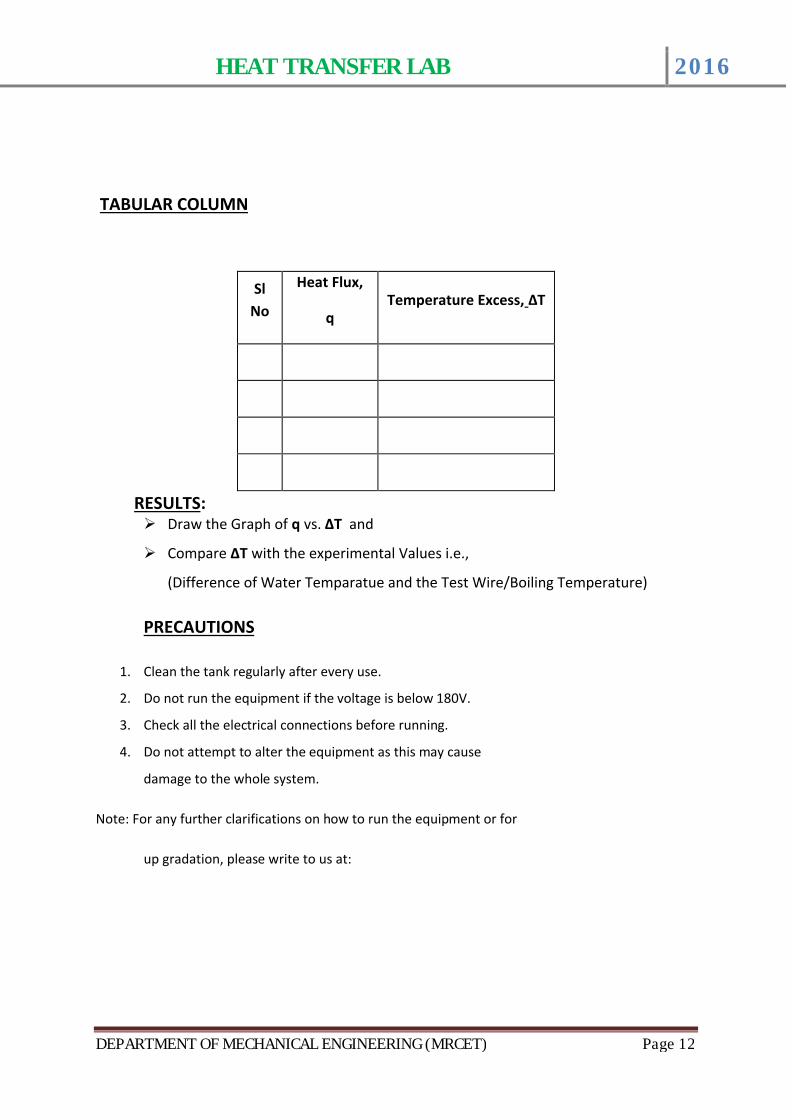
TABULAR COLUMN
Sl No
Heat Flux,
qTemperature Excess, ∆T
RESULTS:ÿ Draw the Graph of q vs. ∆T and
ÿ Compare ∆T with the experimental Values i.e.,
(Difference of Water Temparatue and the Test Wire/Boiling Temperature)
PRECAUTIONS
1. Clean the tank regularly after every use.
2. Do not run the equipment if the voltage is below 180V.
3. Check all the electrical connections before running.
4. Do not attempt to alter the equipment as this may cause
damage to the whole system.
Note: For any further clarifications on how to run the equipment or for
up gradation, please write to us at:
HEAT TRANSFER LAB 2016
DEPARTMENT OF MECHANICAL ENGINEERING (MRCET) Page 13
3.MEASUREMENT OF SURFACE EMMISSIVITY
INTRODUCTION:
Radiation is one of the modes of heat transfer, which does not require any material medium
for its propagation. All bodies can emit radiation & have also the capacity to absorb all or a part of
the radiation coming from the surrounding towards it. The mechanism is assumed to be
electromagnetic in nature and is a result of temperature difference. Thermodynamic considerations
show that an ideal radiator or black body will emit energy at a rate proportional to the fourth power
of the absolute temperature of the body. Other types of surfaces such as glossy painted surface or a
polished metal plate do
not radiate as much energy as the black body , however the total radiation emitted by these bodies
still generally follow the fourth power proportionality. To take account of the gray nature of such
surfaces, the factor called emmissivity (e), which relates the radiation of the gray surface to that of
an ideal black surface, is used. The emissivity of the surface is the ratio of the emissive power of the
surface to the emissive power of the black surface at the same temperature. Emissivity is the
property of the surface and depends upon the nature of the surface and temperature.
DESCRIPTION OF THE APPARATUS:
The setup consists of a 200mm dia two copper plates one surface blackened to get the
effect of the black body and other is platened to give the effect of the gray body. Both the plates
with mica heaters are mounted on the ceramic base covered with chalk powder for maximum heat
transfer. Two Thermocouples are mounted on their surfaces to measure the temperatures of the
surface and one more to measure the enclosure/ambient temperature. This complete arrangement
is fixed in an acrylic chamber for visualization. Temperatures are indicated on the digital
temperature indicator with channel selector to select the temperature point. Heater regulators are
provided to control and monitor the heat input to the system with voltmeter and ammeter for direct
measurement of the heat inputs. The heater controller is made of complete aluminium body having
fuse.
With this, the setup is mounted on an aesthetically designed frame with control panel to
monitor all the processes. The control panel consists of mains on indicator, Aluminium body heater
controllers, change over switches, digital Data logger is used to measure the temperature, voltage
and current of the Black body and grey body and other necessary instrumentation. The whole
arrangement is on the single bench considering all safety and aesthetics factors.
HEAT TRANSFER LAB 2016
DEPARTMENT OF MECHANICAL ENGINEERING (MRCET) Page 14
EXPERIMENTATION:
AIM: The experiment is conducted to determine the emmissivity of the non – black surface and compare with the black body.
PROCEDURE:
1. Give necessary electrical connections and switch on the MCB and switch on the console on
to activate the control panel.
2. Switch On the heater of the black body and set the voltage (say 30V) using the heater
regulator
3. Switch On the heater of the Gray body and set the voltage (say 30V) using the heater
regulator.
4. Observe temperatures of the black body and test surface in close time intervals and adjust
power input to the test plate heater such that both black body and test surface
temperatures are same.
NOTE: This procedure requires trial and error method and one has to wait sufficiently long (say
2hours or longer) to reach a steady state.
5. Wait to attain the steady state.
6. Note down the temperatures at different points and also the voltmeter and ammeter
readings.
7. Tabulate the readings and calculate the surface emmissivity of the non – black surface.
PROCEDURE : COMPUTERIZED
TAKING READINGS – COMPUTERIZED
1. Switch on the panel.
2. Switch on the computer.
3. Open the “ HEAT TRANSFER Software” from the installed location a welcome screen will be
displayed
4. Follow the below steps to operate through software
Once the software is opened, the main screen will be displaced
Now, press “START” button, and the small screen will opened
Enter the parameters listed for particular test under study.
the software starts displaying the calculated values which can be cross verified based on the formulae give after.
HEAT TRANSFER LAB 2016
DEPARTMENT OF MECHANICAL ENGINEERING (MRCET) Page 15
5. Switch On the heater of the black body and set the voltage (say 30V) using the heater
regulator
6. Switch On the heater of the Gray body and set the voltage (say 30V) using the heater
regulator.
7. Observe temperatures of the black body and test surface in close time intervals and adjust
power input to the test plate heater such that both black body and test surface
temperatures are same.
8. Wait to attain the steady state.
9. Click the “store” button to store the value can be viewed anytime later.
10. After completion of the Experiment to press the stop button
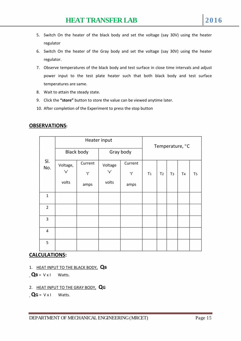
OBSERVATIONS:
Sl. No.
Heater inputTemperature, ∞C
Black body Gray body
Voltage, ‘v’
volts
Current
‘I’
amps
Voltage ‘v’
volts
Current
‘I’
amps
T1 T2 T3 T4 T5
1
2
3
4
5
CALCULATIONS:
1. HEAT INPUT TO THE BLACK BODY, QB
QB = V x I Watts.
2. HEAT INPUT TO THE GRAY BODY, QG
QG = V x I Watts.
HEAT TRANSFER LAB 2016
DEPARTMENT OF MECHANICAL ENGINEERING (MRCET) Page 16
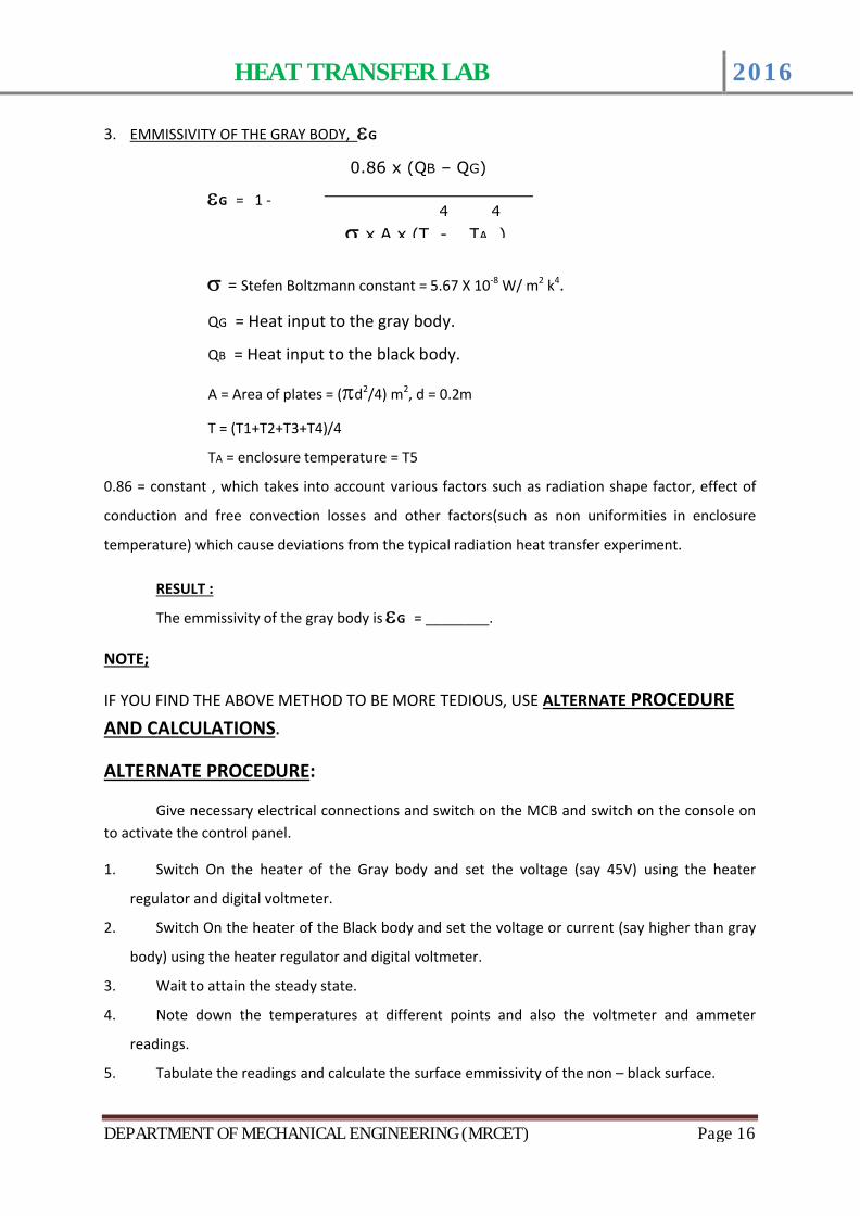
0.86 x (QB – QG)
s x A x (T - TA ) 4 4
3. EMMISSIVITY OF THE GRAY BODY, eG
eG = 1 -
s = Stefen Boltzmann constant = 5.67 X 10⁻⁸ W/ m2 k4.
QG = Heat input to the gray body.
QB = Heat input to the black body.
A = Area of plates = (pd2/4) m2, d = 0.2m
T = (T1+T2+T3+T4)/4
TA = enclosure temperature = T5
0.86 = constant , which takes into account various factors such as radiation shape factor, effect of
conduction and free convection losses and other factors(such as non uniformities in enclosure
temperature) which cause deviations from the typical radiation heat transfer experiment.
RESULT :
The emmissivity of the gray body is eG = ________.
NOTE;
IF YOU FIND THE ABOVE METHOD TO BE MORE TEDIOUS, USE ALTERNATE PROCEDURE AND CALCULATIONS.
ALTERNATE PROCEDURE:
Give necessary electrical connections and switch on the MCB and switch on the console on to activate the control panel.
1. Switch On the heater of the Gray body and set the voltage (say 45V) using the heater
regulator and digital voltmeter.
2. Switch On the heater of the Black body and set the voltage or current (say higher than gray
body) using the heater regulator and digital voltmeter.
3. Wait to attain the steady state.
4. Note down the temperatures at different points and also the voltmeter and ammeter
readings.
5. Tabulate the readings and calculate the surface emmissivity of the non – black surface.
HEAT TRANSFER LAB 2016
DEPARTMENT OF MECHANICAL ENGINEERING (MRCET) Page 17
QG (TB - TA )
QB (TG - TA )
4 4
4
4
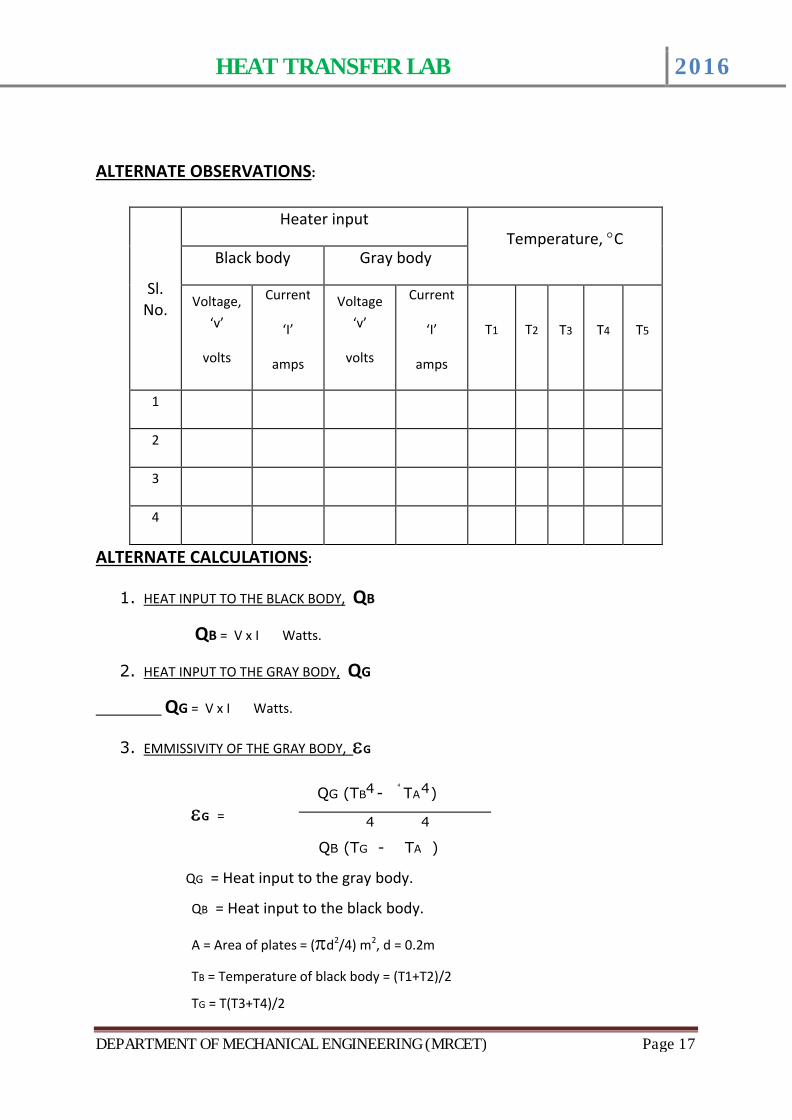
ALTERNATE OBSERVATIONS:
Sl. No.
Heater inputTemperature, ∞C
Black body Gray body
Voltage, ‘v’
volts
Current
‘I’
amps
Voltage ‘v’
volts
Current
‘I’
amps
T1 T2 T3 T4 T5
1
2
3
4
ALTERNATE CALCULATIONS:
1. HEAT INPUT TO THE BLACK BODY, QB
QB = V x I Watts.
2. HEAT INPUT TO THE GRAY BODY, QG
QG = V x I Watts.
3. EMMISSIVITY OF THE GRAY BODY, eG
eG =
QG = Heat input to the gray body.
QB = Heat input to the black body.
A = Area of plates = (pd2/4) m2, d = 0.2m
TB = Temperature of black body = (T1+T2)/2
TG = T(T3+T4)/2
4
HEAT TRANSFER LAB 2016
DEPARTMENT OF MECHANICAL ENGINEERING (MRCET) Page 18
TA = Ambient temperature = T5
4. RESULT :The emissivity of the gray body is eG = ________.
Reference:
1) Heat and Mass transfer by Arora & Domkundwar2) Chemical Engineers’ Handbook, by
Robert H. Perry / Cecil H. ChiltonPublication: McGraw – Hill Book Company (6th edition)
PRECAUTIONS:
1. Check all the electrical connections.
2. Do not run the equipment if the voltage is below 180V.
3. Make sure that heater regulator is at the minimum position before switching on the
console.
4. After finishing the experiment open the acrylic door to remove the heat from the
chamber.
5. Do not attempt to alter the equipment as this may cause damage to the whole system.
HEAT TRANSFER LAB 2016
DEPARTMENT OF MECHANICAL ENGINEERING (MRCET) Page 19
4.HEAT TRANSFER THROUGH FORCED CONVECTION
INTRODUCTION:
Heat transfer can be defined as the transmission of energy from one region to another as a result of temperature difference between them. There are three different modes of heat transfer; namely,
HEAT CONDUCTION : The property which allows the passage for heat energy,
even though its parts are not in motion relative to one
another.
HEAT CONVECTION : The capacity of moving matter to carry heat energy by
actual movement.
HEAT RADIATION : The property of matter to emit or to absorb different kinds
of radiation by electromagnetic waves.
Out of these types of heat transfer the convective heat transfer which of our present
concern, divides into two catagories, Viz.,
NATURAL CONVECTION: If the motion of fluid is caused only due to difference in density
resulting from temperature gradients without the use of pump or fan, then the mechanism
of heat transfer is known as “Natural or Free Convection”.
FORCED CONVECTION:If the motion of fluid is induced by some external means such as a
pump or blower, then the heat transfer process is known as “Forced Convection”.
The newtons law of cooling in convective heat transfer is given by,
q = h A ΔT
Where, q = Heat transfer rate, in watts
A = Surface area of heat flow, in m2
ΔT = Overall temperature difference between the wall and fluid, in
oC
h = Convection heat transfer co-efficient, in watts/m2 oC
This setup has been designed to study heat transfer by forced convection.
HEAT TRANSFER LAB 2016
DEPARTMENT OF MECHANICAL ENGINEERING (MRCET) Page 20
DESCRIPTION OF THE APPARATUS:
The apparatus consists of
Heat exchanger tube made of copper which is thermally insulated outside to prevent heat
transfer losses to the atmosphere.
Band heaters of 500watts capacity.
Heater regulator to supply the regulated power input to the heater.
Data logger is used to measure the Temperature, Voltage ,current and Air flow rat .
Thermocouples at suitable position to measure the temperatures of body and the air.
Blower unit to blow air through the heat exchanger with orifice meter and Differential
Pressure Transducer to measure the air flow rate from the blower. A control valve is provided to
regulate the air flow.
Control panel to house all the instrumentation.
With this the whole arrangement is mounted on an aesthetically
designed self-sustained frame with a separate NOVAPAN Board control panel.
EXPERIMENTATION:
AIM: To determine convective heat transfer coefficient in forced convection.
PROCEDURE : MANUAL
1. Switch on the MCB and then console on switch to activate the control panel.
2. Switch on the blower unit first and adjust the flow of air using wheel valve of blower to a
desired difference in manometer.
3. Switch on the heater and set the voltage (say 80V) using the heater regulator.
4. Wait for reasonable time to allow temperatures to reach steady state.
5. Measure the voltage, current and temperatures from T1 to T6 at known time interval.
6. Calculate the convective heat transfer co-efficient using the procedure given.
7. Repeat the experiment for different values of power input to the heater and blower air flow
rates.
HEAT TRANSFER LAB 2016
DEPARTMENT OF MECHANICAL ENGINEERING (MRCET) Page 21
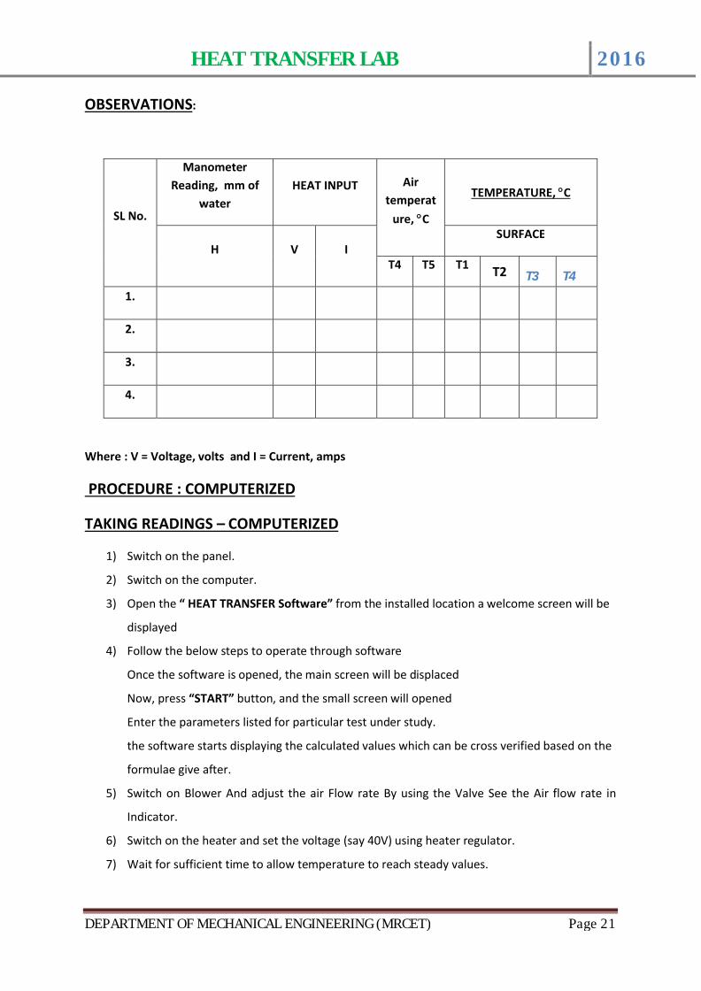
OBSERVATIONS:
SL No.
Manometer Reading, mm of
waterHEAT INPUT Air
temperature, ∞C
TEMPERATURE, ∞C
H V ISURFACE
T4 T5 T1 T2 T3 T4
1.
2.
3.
4.
Where : V = Voltage, volts and I = Current, amps
PROCEDURE : COMPUTERIZED
TAKING READINGS – COMPUTERIZED
1) Switch on the panel.
2) Switch on the computer.
3) Open the “ HEAT TRANSFER Software” from the installed location a welcome screen will be
displayed
4) Follow the below steps to operate through software
Once the software is opened, the main screen will be displaced
Now, press “START” button, and the small screen will opened
Enter the parameters listed for particular test under study.
the software starts displaying the calculated values which can be cross verified based on the
formulae give after.
5) Switch on Blower And adjust the air Flow rate By using the Valve See the Air flow rate in
Indicator.
6) Switch on the heater and set the voltage (say 40V) using heater regulator.
7) Wait for sufficient time to allow temperature to reach steady values.
HEAT TRANSFER LAB 2016
DEPARTMENT OF MECHANICAL ENGINEERING (MRCET) Page 22
8) Repeat the experiment for different heat inputs and also for horizontal position with
different heat inputs.
9) Wait to attain the steady state.
10) Click the “store” button to store the value can be viewed anytime later.
11) After completion of the Experiment to press the stop button.
CALCULATIONS:
PRACTICAL
1. h =
where, Q = heat given to the heater = V x I watts.
A = Area of the tube surface = p d L
d = 0.036m and L = 0.5m
Ti = mean temperature = (T1+T2+T3+T4)/4
To = . (T5+T6)/3
THEORETICAL
h = (0.023 x Pr x Re x k) / D
Where,
rVD
Re = -----------
m
where , D = inner diameter of the tube = 0.036
V = m/s
Q
A (Ti -To)
0.4 0.8
m Cp
Pr = ---------
K
mass flow rate of airFlow area
HEAT TRANSFER LAB 2016
DEPARTMENT OF MECHANICAL ENGINEERING (MRCET) Page 23
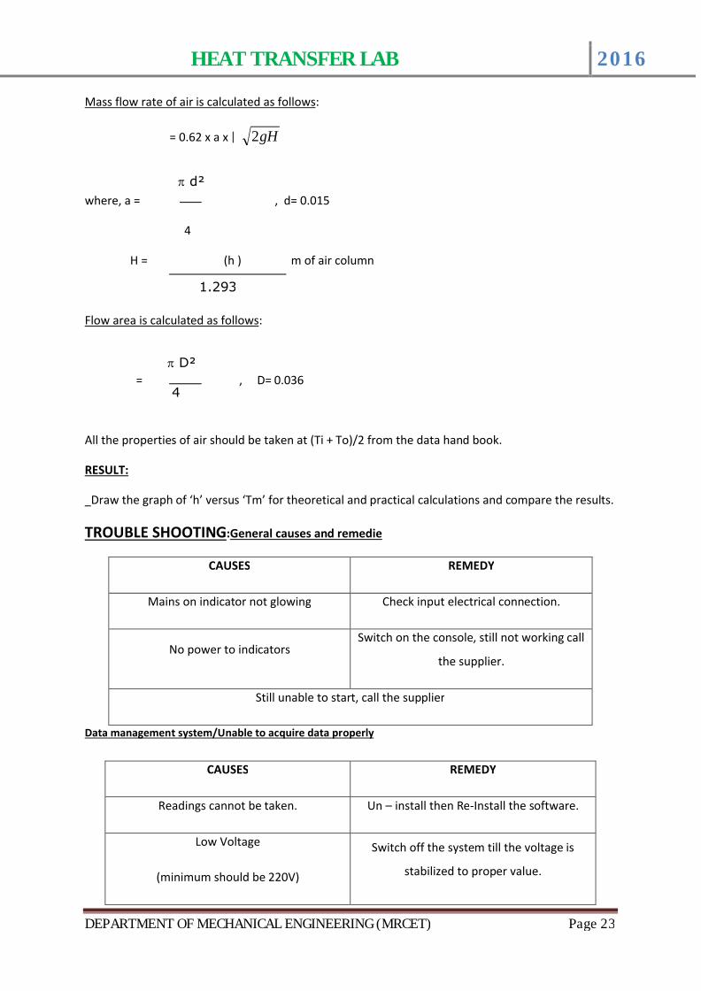
Mass flow rate of air is calculated as follows:
= 0.62 x a x gH2
where, a = , d= 0.015
4
H = (h ) m of air column
Flow area is calculated as follows:
= , D= 0.036
All the properties of air should be taken at (Ti + To)/2 from the data hand book.
RESULT:
Draw the graph of ‘h’ versus ‘Tm’ for theoretical and practical calculations and compare the results.
TROUBLE SHOOTING:General causes and remedie
CAUSES REMEDY
Mains on indicator not glowing Check input electrical connection.
No power to indicatorsSwitch on the console, still not working call
the supplier.
Still unable to start, call the supplier
Data management system/Unable to acquire data properly
CAUSES REMEDY
Readings cannot be taken. Un – install then Re-Install the software.
Low Voltage
(minimum should be 220V)
Switch off the system till the voltage is
stabilized to proper value.
p d²
1.293
p D²
4
HEAT TRANSFER LAB 2016
DEPARTMENT OF MECHANICAL ENGINEERING (MRCET) Page 24
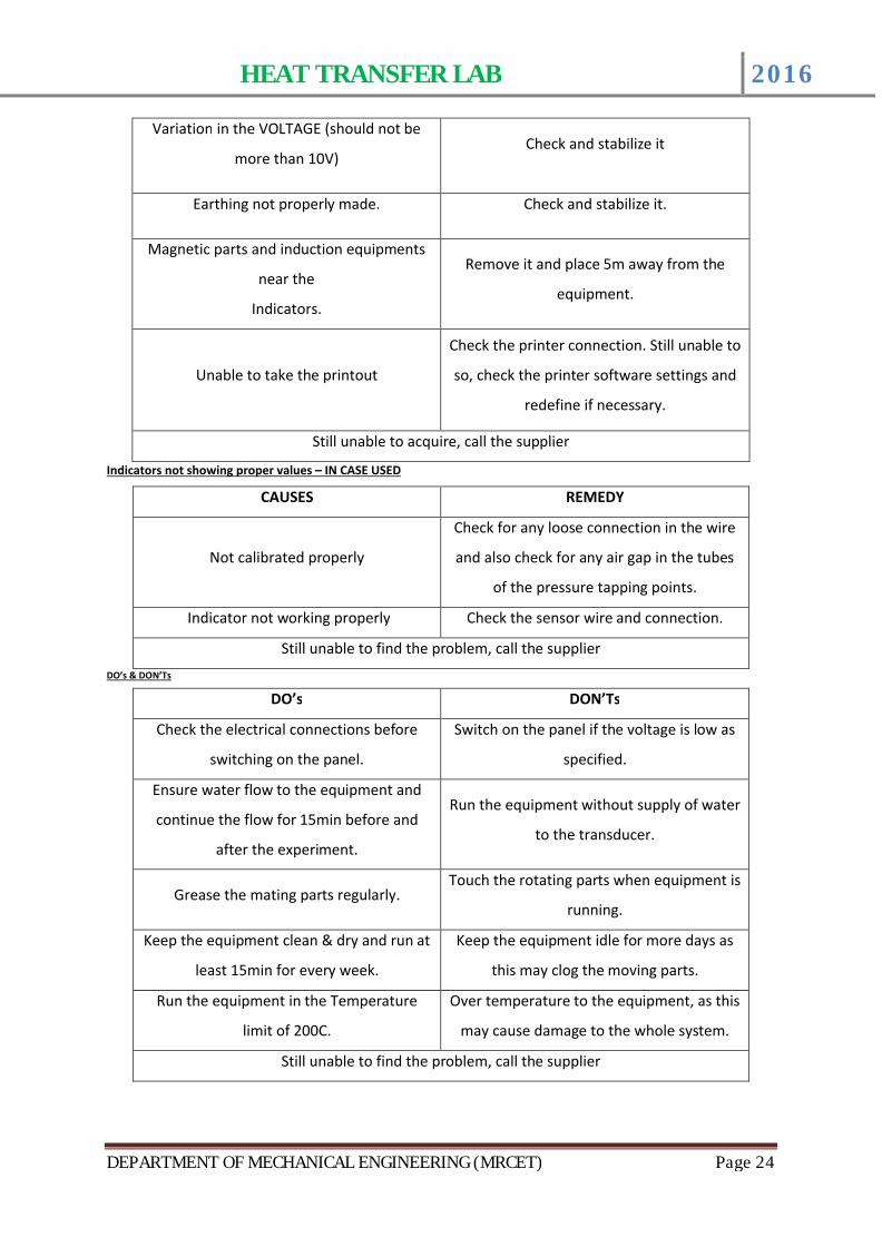
Variation in the VOLTAGE (should not be
more than 10V)Check and stabilize it
Earthing not properly made. Check and stabilize it.
Magnetic parts and induction equipments
near the
Indicators.
Remove it and place 5m away from the
equipment.
Unable to take the printout
Check the printer connection. Still unable to
so, check the printer software settings and
redefine if necessary.
Still unable to acquire, call the supplier
Indicators not showing proper values – IN CASE USED
CAUSES REMEDY
Not calibrated properly
Check for any loose connection in the wire
and also check for any air gap in the tubes
of the pressure tapping points.
Indicator not working properly Check the sensor wire and connection.
Still unable to find the problem, call the supplier
DO’s & DON’Ts
DO’s DON’Ts
Check the electrical connections before
switching on the panel.
Switch on the panel if the voltage is low as
specified.
Ensure water flow to the equipment and
continue the flow for 15min before and
after the experiment.
Run the equipment without supply of water
to the transducer.
Grease the mating parts regularly.Touch the rotating parts when equipment is
running.
Keep the equipment clean & dry and run at
least 15min for every week.
Keep the equipment idle for more days as
this may clog the moving parts.
Run the equipment in the Temperature
limit of 200C.
Over temperature to the equipment, as this
may cause damage to the whole system.
Still unable to find the problem, call the supplier
HEAT TRANSFER LAB 2016
DEPARTMENT OF MECHANICAL ENGINEERING (MRCET) Page 25
LIMITATIONS & PRECAUTIONS
1) Maximum Load is limited to 150V.
2) This is a general equipment for study in undergraduate level, for consideration of higher level
studies you can add any extra parameter required. For adding the parameters call the supplier.
3) Don’t run the equipment if the voltage is less than 180V.
4) 230V, 1ph with neutral and proper earthing to be provided.
5) Don’t alter the equipment without the supervision of the supplier.
Reference:
1) Heat and Mass transfer by Arora & Domkundwar2) Chemical Engineers’ Handbook, byRobert H. Perry / Cecil H. Chilton
Publication: McGraw – Hill Book Company (6th edition)
HEAT TRANSFER LAB 2016
DEPARTMENT OF MECHANICAL ENGINEERING (MRCET) Page 26
5.HEAT PIPE DEMONSTRATIONINTRODUCTION:
One of the main objectives of energy conversion systems is to transfer energy from a receiver to
some other location where it can be used to heat a working fluid. The heat pipe is a novel device
that can transfer large quantities of heat through small surface areas with small temperature
differences. Here in this equipment an attempt has been made to show the students, how the heat
pipe works with different methods.
DESCRIPTION OF THE APPARATUS:
The apparatus consists of a Solid Copper Rod of diameter (d) 25mm and length (L) 500mm with a
Source at one end and condenser at other end.
Similarly, Hollow copper pipe without wick and with wick (SS mesh of 180microns) with same outer
dia and length is provided.
Thermocouples are fixed on the tube surface with a phase angle of 90∞ on each pipe.
Control panel instrumentation consists of:
e. Digital Temperature Indicator with channel selector.
f. Digital Voltmeter & Ammeter for power measurement.
g. Heater regulator to regulate the input power.
With this, the setup is mounted on an aesthetically designed MS Powder coated frame with
MOVAPAN Board control panel to monitor all the processes considering all safety and aesthetics
factors.
EXPERIMENTATION:
AIM:
To determine the axial heat flux in a heat pipe using water as the working fluid with that of a solid
copper with different temperatures.
PROCEDURE:
1) Provide the necessary electrical connection and then CONSOLE ON switch.
2) Switch on the heater and set the voltage (say 40V) using heater regulator and the digital voltmeter.
3) Wait for sufficient time to allow temperature to reach steady values.
4) Note down the Temperatures 1 to 6 using the channel selector and digital temperature indicator.
5) Note down the ammeter and voltmeter readings.
6) Calculate the axial heat flux for all the pipes.
7) Repeat the experiment for different heat inputs and compare the results.
HEAT TRANSFER LAB 2016
DEPARTMENT OF MECHANICAL ENGINEERING (MRCET) Page 27
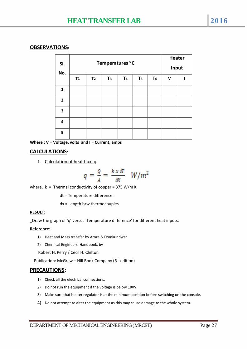
OBSERVATIONS:
Sl.
No.
Temperatures ∞CHeater
Input
T1 T2 T3 T4 T5 T6 V I
1
2
3
4
5
Where : V = Voltage, volts and I = Current, amps
CALCULATIONS:
1. Calculation of heat flux, q
where, k = Thermal conductivity of copper = 375 W/m K
dt = Temperature difference.
dx = Length b/w thermocouples.
RESULT:
Draw the graph of ‘q’ versus ‘Temperature difference’ for different heat inputs.
Reference:
1) Heat and Mass transfer by Arora & Domkundwar
2) Chemical Engineers’ Handbook, by
Robert H. Perry / Cecil H. Chilton
Publication: McGraw – Hill Book Company (6th edition)
PRECAUTIONS:
1) Check all the electrical connections.
2) Do not run the equipment if the voltage is below 180V.
3) Make sure that heater regulator is at the minimum position before switching on the console.
4) Do not attempt to alter the equipment as this may cause damage to the whole system.
HEAT TRANSFER LAB 2016
DEPARTMENT OF MECHANICAL ENGINEERING (MRCET) Page 28
6.HEAT TRANSFER THROUGH LAGGED PIPEINTRODUCTION:
The costs involved in insulting either heated or refrigerated equipment, air-conditioned
rooms, pipes, ducts, tanks, and vessels are of a magnitude to warrant careful consideration of the
type and quantity of insulation to be used. Economic thickness is defined as the minimum annual
value of the sum of the cost of heat loss plus the cost of insulation, or, in more general terms, as the
thickness, of a given insulation that will save the greatest cost of energy while paying for itself within
an assigned period of time. At low values of thickness, the amortized annual cost of insulation is low,
but the annual cost of heat energy is high. Additional thickness adds to the cost of insulation but
reduces the loss of heat energy, and therefore, its cost. At some value of insulation thickness, the
sum of the cost of insulation and the cost of heat loss will be a minimum, curve C rises because the
increased cost insulation is no longer offset by the reduced cost of heat loss.
The calculation of economic thickness for an industrial installation is not easy, owing to the large
number of variables and separate calculations involved. This has all been reduced to manual form in
“How to determine economic thickness of insulation”, published by National Insulation
Manufacturers Association, New York.
CRITICAL THICKNESS OF INSULATION:
It must not be taken for granted that insulation only retards the rate of heat flow. The
addition of small amount of insulation to small diameter wires or tubes frequently increases the rate
of heat flow through the tube to the ambient air. It was shown elsewhere in the standard books with
experiment that the rate of heat loss was increased by the addition of the asbestos sheet.
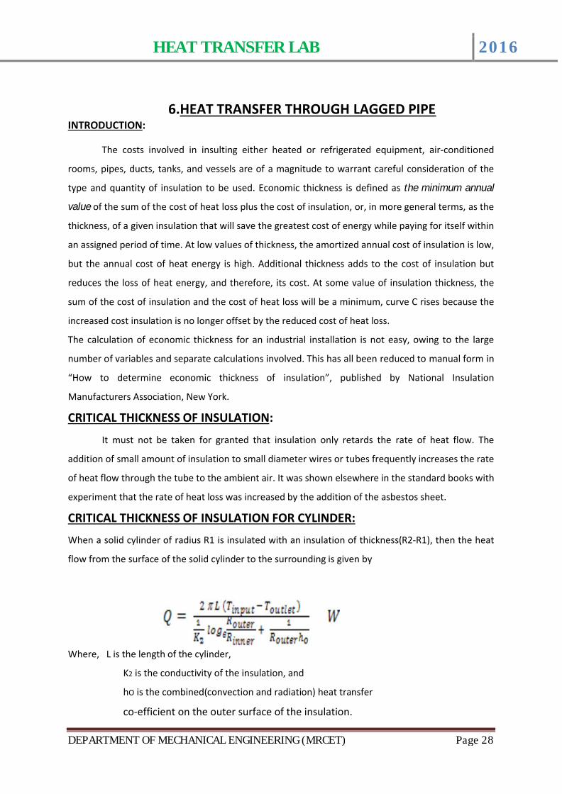
CRITICAL THICKNESS OF INSULATION FOR CYLINDER:
When a solid cylinder of radius R1 is insulated with an insulation of thickness(R2-R1), then the heat
flow from the surface of the solid cylinder to the surrounding is given by
Where, L is the length of the cylinder,
K2 is the conductivity of the insulation, and
hO is the combined(convection and radiation) heat transfer
co-efficient on the outer surface of the insulation.
HEAT TRANSFER LAB 2016
DEPARTMENT OF MECHANICAL ENGINEERING (MRCET) Page 29
DESCRIPTION:
The experimental set-up consists of a copper pipe of 38mm diameter divided into four zones
of 150mm each. The zone 1 is a bare pipe, and zone 2 is wound with asbestos rope to 60mm dia, and
that of zone 3 to 90mm dia and zone 4 to 110mm dia. The heater of 500 watts is centred along the
length of the pipe (150x4=600mm).
Heater regulator to supply the regulated power input to the heater. Digital Voltmeter and Ammeter
to measure poser input ot the heater. Thermocouples at suitable position to measure the
temperatures of body and the air. Digital Temperature Indicator with channel selector to measure
the temperatures.
Control panel to house all the instrumentation.
With this the whole arrangement is mounted on an aesthetically
designed self-sustained MS powder coated frame with a separate NOVAPAN Board control panel.
EXPERIMENTATION:
AIM:
To determine combined convective and radiation heat transfer coefficient at each zone and compare
them to decide the critical thickness of insulation.
PROCEDURE:
1. Switch on the MCB and then console on switch to activate the control panel.
2. Switch on the heater and set the voltage (say 40V) using the heater regulator and digital voltmeter.
3. Wait for reasonable time to allow temperatures to reach steady state.
4. Measure the voltage, current and temperatures from T1 to T7 at known time interval.
5. Calculate the heat transfer co-efficient using the procedure given.
6. Repeat the experiment for different values of power input to the heater.
HEAT TRANSFER LAB 2016
DEPARTMENT OF MECHANICAL ENGINEERING (MRCET) Page 30
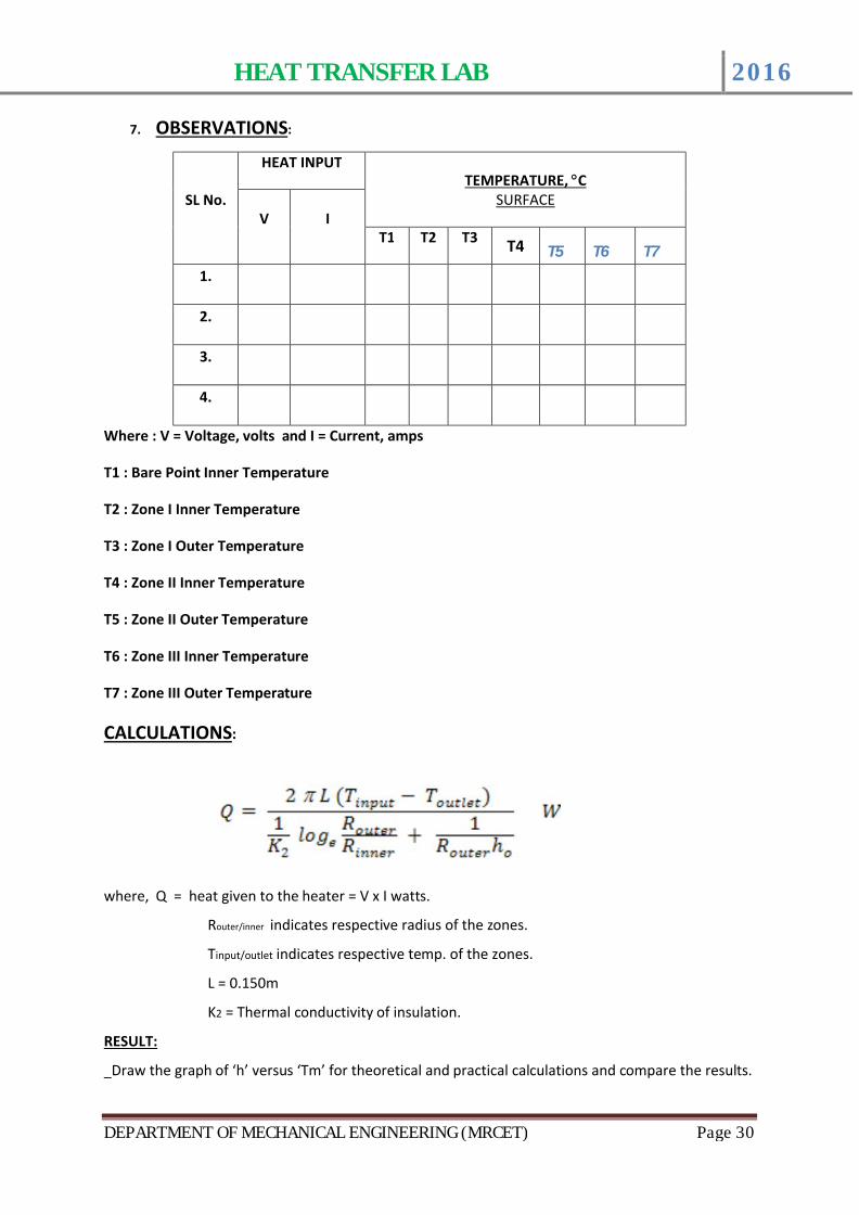
7. OBSERVATIONS:
SL No.
HEAT INPUTTEMPERATURE, ∞C
SURFACEV I
T1 T2 T3 T4 T5 T6 T7
1.
2.
3.
4.
Where : V = Voltage, volts and I = Current, amps
T1 : Bare Point Inner Temperature
T2 : Zone I Inner Temperature
T3 : Zone I Outer Temperature
T4 : Zone II Inner Temperature
T5 : Zone II Outer Temperature
T6 : Zone III Inner Temperature
T7 : Zone III Outer Temperature
CALCULATIONS:
where, Q = heat given to the heater = V x I watts.
Router/inner indicates respective radius of the zones.
Tinput/outlet indicates respective temp. of the zones.
L = 0.150m
K2 = Thermal conductivity of insulation.
RESULT:
Draw the graph of ‘h’ versus ‘Tm’ for theoretical and practical calculations and compare the results.
HEAT TRANSFER LAB 2016
DEPARTMENT OF MECHANICAL ENGINEERING (MRCET) Page 31
Reference:
1. Heat and Mass transfer by Arora & Domkundwar
2. Chemical Engineers’ Handbook, by
Robert H. Perry / Cecil H. Chilton
Publication: McGraw – Hill Book Company (6th edition)
PRECAUTIONS:
1. Check all the electrical connections.
2. Do not run the equipment if the voltage is below 180V.
3. Make sure that heater regulator is at the minimum position before switching on the console.
4. Do not attempt to alter the equipment as this may cause damage to the whole system.
HEAT TRANSFER LAB 2016
DEPARTMENT OF MECHANICAL ENGINEERING (MRCET) Page 32
7.HEAT TRANSFER THROUGH NATURAL CONVECTIONINTRODUCTION:
There are certain situations in which the fluid motion is produced due to change in density
resulting from temperature gradients. The mechanism of heat transfer in these situations is called
free or natural convection. Free convection is the principal mode of heat transfer from pipes,
transmission lines, refrigerating coils, hot radiators etc.
The movement of fluid in free convection is due to the fact that the fluid particles in the immediate
vicinity of the hot object become warmer than the surrounding fluid resulting in a local change of
density. The colder fluid creating convection currents would replace the warmer fluid. These
currents originate when a body force (gravitational, centrifugal, electrostatic etc) acts on a fluid in
which there are density gradients. The force, which induces these convection currents, is called a
buoyancy force that is due to the presence of a density gradient with in the fluid and a body force.
Grashoffs number a dimensionless quantity plays a very important role in natural convection.
DESCRIPTION OF THE APPARATUS:
The apparatus consists of a Chromium plated Copper tube of diameter (d) 38mm and length
(L) 500mm with a Special electrical heater along the axis of the tube for uniform heating.
Four thermocouples are fixed on the tube surface with a phase angle of 90∞.
An arrangement to change the position of the tube to vertical or horizontal position is provided.
Front transparent acrylic enclosure to minimize the disturbances of the surrounding and also for
safety of the tube when not in use.
Contol panel instrumentation consists of:
h. Mains on, console on
i. Data logger is used to measure the Temp, Voltage and current.
j. Heater regulator to regulate the input power.
With this, the setup is mounted on an aesthetically designed frame with NOVAPAN Board
control panel to monitor all the processes considering all safety and aesthetics factors.
HEAT TRANSFER LAB 2016
DEPARTMENT OF MECHANICAL ENGINEERING (MRCET) Page 33
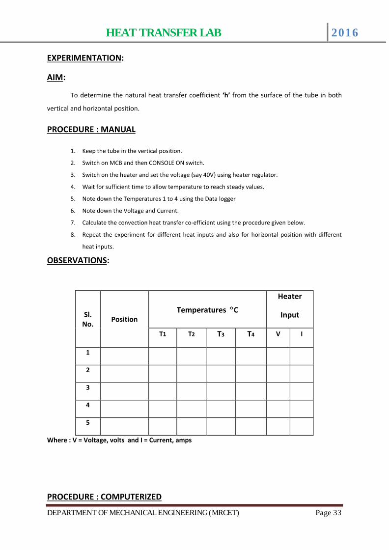
EXPERIMENTATION:
AIM:
To determine the natural heat transfer coefficient ‘h’ from the surface of the tube in both
vertical and horizontal position.
PROCEDURE : MANUAL
1. Keep the tube in the vertical position.
2. Switch on MCB and then CONSOLE ON switch.
3. Switch on the heater and set the voltage (say 40V) using heater regulator.
4. Wait for sufficient time to allow temperature to reach steady values.
5. Note down the Temperatures 1 to 4 using the Data logger
6. Note down the Voltage and Current.
7. Calculate the convection heat transfer co-efficient using the procedure given below.
8. Repeat the experiment for different heat inputs and also for horizontal position with different
heat inputs.
OBSERVATIONS:
Sl. No. Position
Temperatures ∞C
Heater
Input
T1 T2 T3 T4 V I
1
2
3
4
5
Where : V = Voltage, volts and I = Current, amps
PROCEDURE : COMPUTERIZED
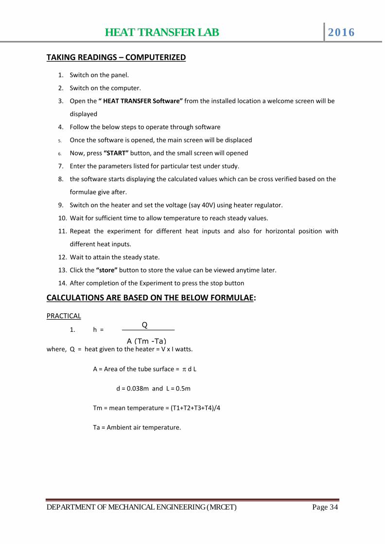
HEAT TRANSFER LAB 2016
DEPARTMENT OF MECHANICAL ENGINEERING (MRCET) Page 34
TAKING READINGS – COMPUTERIZED
1. Switch on the panel.
2. Switch on the computer.
3. Open the “ HEAT TRANSFER Software” from the installed location a welcome screen will be
displayed
4. Follow the below steps to operate through software
5. Once the software is opened, the main screen will be displaced
6. Now, press “START” button, and the small screen will opened
7. Enter the parameters listed for particular test under study.
8. the software starts displaying the calculated values which can be cross verified based on the
formulae give after.
9. Switch on the heater and set the voltage (say 40V) using heater regulator.
10. Wait for sufficient time to allow temperature to reach steady values.
11. Repeat the experiment for different heat inputs and also for horizontal position with
different heat inputs.
12. Wait to attain the steady state.
13. Click the “store” button to store the value can be viewed anytime later.
14. After completion of the Experiment to press the stop button
CALCULATIONS ARE BASED ON THE BELOW FORMULAE:
PRACTICAL
1. h =
where, Q = heat given to the heater = V x I watts.
A = Area of the tube surface = p d L
d = 0.038m and L = 0.5m
Tm = mean temperature = (T1+T2+T3+T4)/4
Ta = Ambient air temperature.
Q
A (Tm -Ta)
HEAT TRANSFER LAB 2016
DEPARTMENT OF MECHANICAL ENGINEERING (MRCET) Page 35
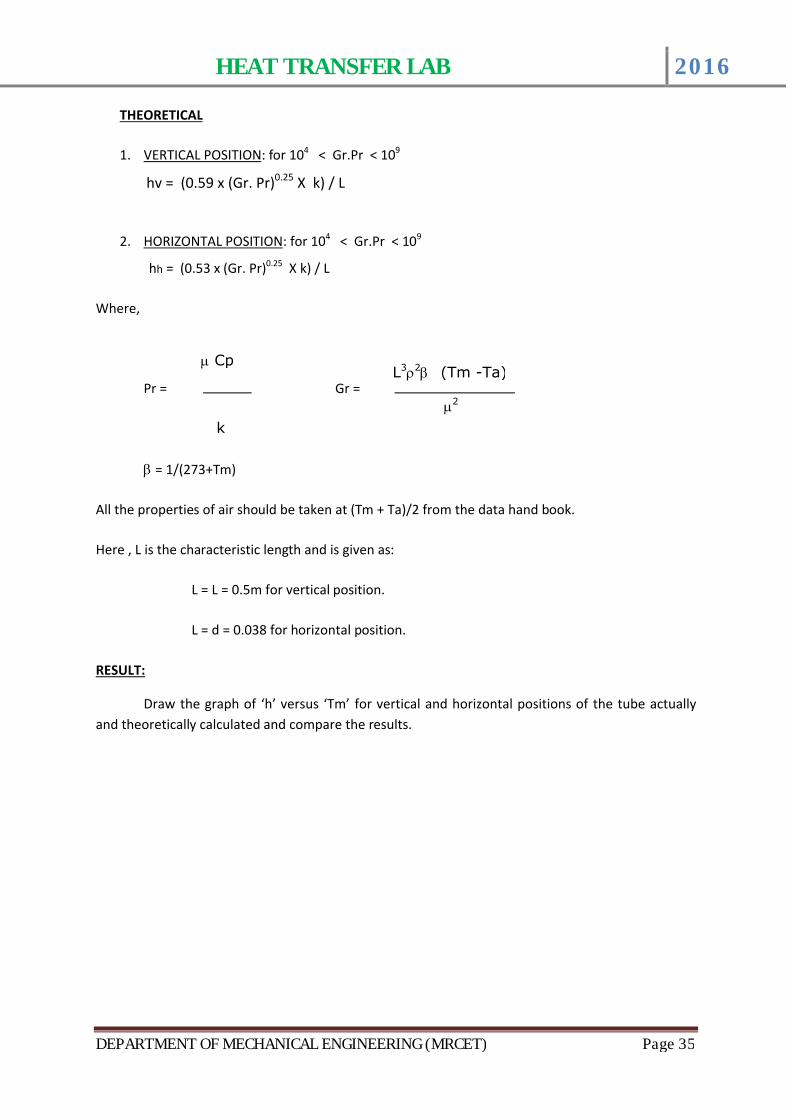
THEORETICAL
1. VERTICAL POSITION: for 104 < Gr.Pr < 109
hv = (0.59 x (Gr. Pr)0.25 X k) / L
2. HORIZONTAL POSITION: for 104 < Gr.Pr < 109
hh = (0.53 x (Gr. Pr)0.25 X k) / L
Where,
Pr = Gr =
b = 1/(273+Tm)
All the properties of air should be taken at (Tm + Ta)/2 from the data hand book.
Here , L is the characteristic length and is given as:
L = L = 0.5m for vertical position.
L = d = 0.038 for horizontal position.
RESULT:
Draw the graph of ‘h’ versus ‘Tm’ for vertical and horizontal positions of the tube actually and theoretically calculated and compare the results.
m Cp
k
L3r2b (Tm -Ta)
m2
HEAT TRANSFER LAB 2016
DEPARTMENT OF MECHANICAL ENGINEERING (MRCET) Page 36
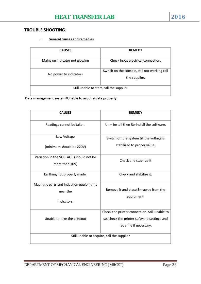
TROUBLE SHOOTING:
o General causes and remedies
CAUSES REMEDY
Mains on indicator not glowing Check input electrical connection.
No power to indicatorsSwitch on the console, still not working call
the supplier.
Still unable to start, call the supplier
Data management system/Unable to acquire data properly
CAUSES REMEDY
Readings cannot be taken. Un – install then Re-Install the software.
Low Voltage
(minimum should be 220V)
Switch off the system till the voltage is
stabilized to proper value.
Variation in the VOLTAGE (should not be
more than 10V)Check and stabilize it
Earthing not properly made. Check and stabilize it.
Magnetic parts and induction equipments
near the
Indicators.
Remove it and place 5m away from the
equipment.
Unable to take the printout
Check the printer connection. Still unable to
so, check the printer software settings and
redefine if necessary.
Still unable to acquire, call the supplier
HEAT TRANSFER LAB 2016
DEPARTMENT OF MECHANICAL ENGINEERING (MRCET) Page 37
o Indicators not showing proper values – IN CASE USED
CAUSES REMEDY
Not calibrated properly
Check for any loose connection in the wire
and also check for any air gap in the tubes
of the pressure tapping points.
Indicator not working properly Check the sensor wire and connection.
Still unable to find the problem, call the supplier
o DO’s & DON’Ts
DO’s DON’Ts
Check the electrical connections before
switching on the panel.
Switch on the panel if the voltage is low as
specified.
Ensure water flow to the equipment and
continue the flow for 15min before and
after the experiment.
Run the equipment without supply of water
to the transducer.
Grease the mating parts regularly.Touch the rotating parts when equipment is
running.
Keep the equipment clean and run at least
15min for every week.
Keep the equipment idle for more days as
this may clog the moving parts.
Run the equipment in the Temperature
limit of 200C.
Over temperature to the equipment, as this
may cause damage to the whole system.
Still unable to find the problem, call the supplier
HEAT TRANSFER LAB 2016
DEPARTMENT OF MECHANICAL ENGINEERING (MRCET) Page 38
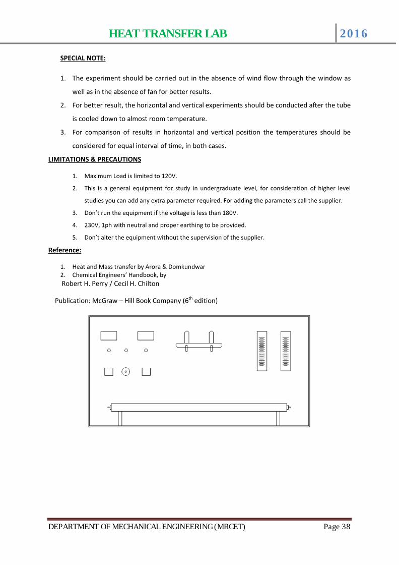
SPECIAL NOTE:
1. The experiment should be carried out in the absence of wind flow through the window as
well as in the absence of fan for better results.
2. For better result, the horizontal and vertical experiments should be conducted after the tube
is cooled down to almost room temperature.
3. For comparison of results in horizontal and vertical position the temperatures should be
considered for equal interval of time, in both cases.
LIMITATIONS & PRECAUTIONS
1. Maximum Load is limited to 120V.
2. This is a general equipment for study in undergraduate level, for consideration of higher level
studies you can add any extra parameter required. For adding the parameters call the supplier.
3. Don’t run the equipment if the voltage is less than 180V.
4. 230V, 1ph with neutral and proper earthing to be provided.
5. Don’t alter the equipment without the supervision of the supplier.
Reference:
1. Heat and Mass transfer by Arora & Domkundwar2. Chemical Engineers’ Handbook, byRobert H. Perry / Cecil H. Chilton
Publication: McGraw – Hill Book Company (6th edition)
HEAT TRANSFER LAB 2016
DEPARTMENT OF MECHANICAL ENGINEERING (MRCET) Page 39
8.PARALLEL & COUNTER FLOWHEAT EXCHANGERINTRODUCTION:
Heat exchangers are devices in which heat is transferred from one fluid to another. The
fluids may be in direct contact with each other or separated by a solid wall. Heat Exchangers can be
classified based on its principle of operation and the direction of flow. The temperature of the fluids
changes in the direction of flow and consequently there occurs a change in the thermal head causing
the flow of heat.
The temperatures profiles at the two fluids in parallel and counter flow are curved and have
logarithmic variations. LMTD is less than the arithmetic mean temperature difference. So, it is always
safer for the designer to use LMTD so as to provide larger heating surface for a certain amount of
heat transfer.
DESCRIPTION OF THE APPARATUS:
The apparatus consists of concentric tubes. The inner tube is made of copper while the outer tube is made of Stainless Steel. Insulation is provided with mica sheet and asbestos rope for effective heat transfer.
Provision has been made for hot water generation by means of geyser.
Change - Over Mechanism is provided to change the direction of flow of cold water in a single operation.
ACRYLIC Rotameters of specific range is used for direct measurement of water flow rate.
Thermocouples are placed at appropriate positions which carry the signals to the
temperature indicator. A data logger indicator is provided to measure the temperature.
The whole arrangement is mounted on an Aesthetically designed self sustained sturdy
frame made of NOVAPAN board control panel. The control panel houses all the indicators,
accessories and necessary instrumentations.
HEAT TRANSFER LAB 2016
DEPARTMENT OF MECHANICAL ENGINEERING (MRCET) Page 40
EXPERIMENTATION:
AIM:
To determine LMTD & Effectiveness of the heat exchanger under parallel and counter Flow arrangement.
PROCEDURE:
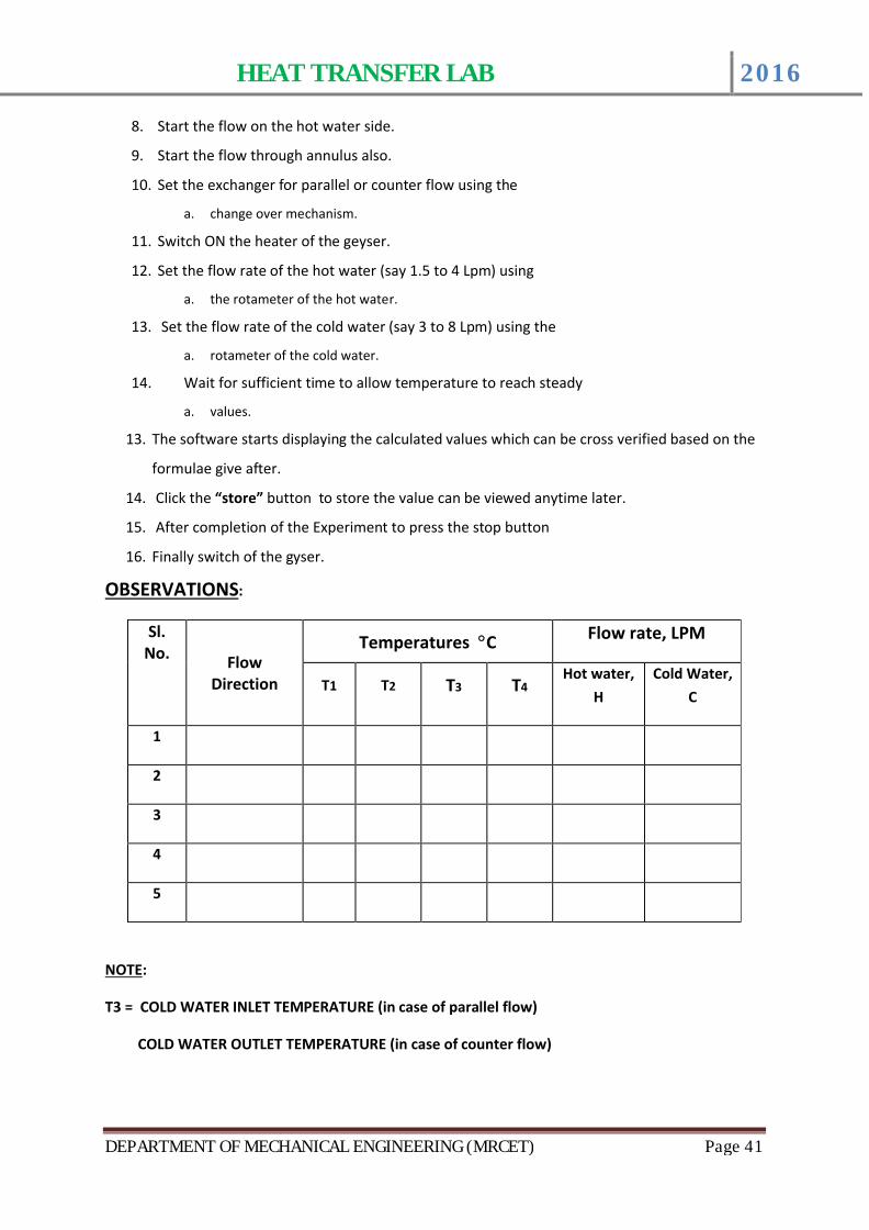
1. Switch ON mains and the CONSOLE.
2. Start the flow on the hot water side.
3. Start the flow through annulus also.
4. Set the exchanger for parallel or counter flow using the
a. change over mechanism.
5. Switch ON the heater of the geyser.
6. Set the flow rate of the hot water (say 1.5 to 4 Lpm) using
a. the rotameter of the hot water.
7. Set the flow rate of the cold water (say 3 to 8 Lpm) using the
a. rotameter of the cold water.
8. Wait for sufficient time to allow temperature to reach steady
a. values.
9. Note down the Temperatures 1 to 4 using the Scanner.
10. Note down the flow rates of the water and tabulate.
11. Now, change the direction of flow for the same flow rates and
a. repeat the steps 9 to 11.
12. Repeat the experiment for different flow rates of water.
PROCEDURE : COMPUTERIZED
TAKING READINGS – COMPUTERIZED
1. Switch on the panel.
2. Switch on the computer.
3. Open the “ HEAT TRANSFER Software” from the installed location a welcome screen will be
displayed
4. Follow the below steps to operate through software
5. Once the software is opened, the main screen will be displaced
6. Now, press “START” button, and the small screen will opened
7. Enter the parameters listed for particular test under study.
HEAT TRANSFER LAB 2016
DEPARTMENT OF MECHANICAL ENGINEERING (MRCET) Page 41
8. Start the flow on the hot water side.
9. Start the flow through annulus also.
10. Set the exchanger for parallel or counter flow using the
a. change over mechanism.
11. Switch ON the heater of the geyser.
12. Set the flow rate of the hot water (say 1.5 to 4 Lpm) using
a. the rotameter of the hot water.
13. Set the flow rate of the cold water (say 3 to 8 Lpm) using the
a. rotameter of the cold water.
14. Wait for sufficient time to allow temperature to reach steady
a. values.
13. The software starts displaying the calculated values which can be cross verified based on the
formulae give after.
14. Click the “store” button to store the value can be viewed anytime later.
15. After completion of the Experiment to press the stop button
16. Finally switch of the gyser.
OBSERVATIONS:
Sl. No. Flow
Direction
Temperatures ∞C Flow rate, LPM
T1 T2 T3 T4Hot water,
HCold Water,
C
1
2
3
4
5
NOTE:
T3 = COLD WATER INLET TEMPERATURE (in case of parallel flow)
COLD WATER OUTLET TEMPERATURE (in case of counter flow)
HEAT TRANSFER LAB 2016
DEPARTMENT OF MECHANICAL ENGINEERING (MRCET) Page 42
T4 = COLD WATER OUTLET TEMPERATURE (in case of parallel flow)
COLD WATER INLET TEMPERATURE (in case of counter flow)
T1 = HOT WATER INLET TEMPERATURE.
T2 = HOT WATER OUTLET TEMERATURE.
CALCULATIONS:
1. HEAT TRANSFER RATE ,Q
Q =
WHERE,
QH = heat transfer rate from hot water and is given by:
= mH x CPH x (T1 – T2) W
Where,
mh = mass flow rate of hot water = H/60 kg/sec.
CPH = Specific heat of hot water from table at temp. (T1+T2)/2
QC = heat transfer rate from cold water and is given by:
= mC x CPC x (T4 – T3) W (for parallel flow)
= mC x CPC x (T3 – T4) W (for counter flow)
Where,
mC = mass flow rate of cold water = C/60 kg/sec.
CPC = Specific heat of cold water from table at temp. (T3+T4)/2
2. LMTD – Logarithmic mean temperature difference:
DTM =
Where,
DTI = (T1 - T3 ) for parallel flow
DTI = (T1 - T4 ) for counter flow
DTO = (T2 - T4 ) for parallel flow
DTO = (T2 - T3 ) for counter flow
DTI - DTO
ln(DTI/DTO)
HEAT TRANSFER LAB 2016
DEPARTMENT OF MECHANICAL ENGINEERING (MRCET) Page 43
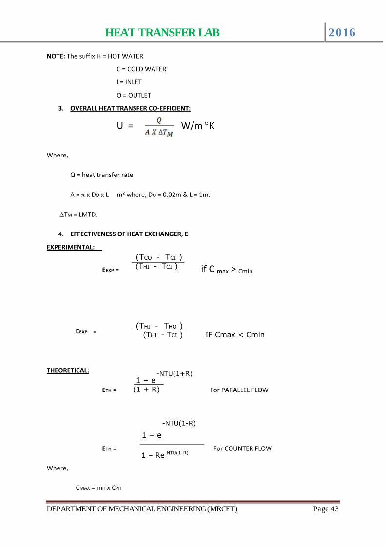
NOTE: The suffix H = HOT WATER
C = COLD WATER
I = INLET
O = OUTLET
3. OVERALL HEAT TRANSFER CO-EFFICIENT:
U = W/m ∞K
Where,
Q = heat transfer rate
A = p x DO x L m² where, DO = 0.02m & L = 1m.
DTM = LMTD.
4. EFFECTIVENESS OF HEAT EXCHANGER, E
EXPERIMENTAL:
EEXP = if C max > Cmin
EEXP =
THEORETICAL:
ETH = For PARALLEL FLOW
ETH = For COUNTER FLOW
Where,
CMAX = mH x CPH
(TCO - TCI )(THI - TCI )
(THI - THO )(THI - TCI ) IF Cmax < Cmin
1 – e(1 + R)
-NTU(1+R)
1 – e
1 – Re-NTU(1-R)
-NTU(1-R)
NTU (1 R)
HEAT TRANSFER LAB 2016
DEPARTMENT OF MECHANICAL ENGINEERING (MRCET) Page 44
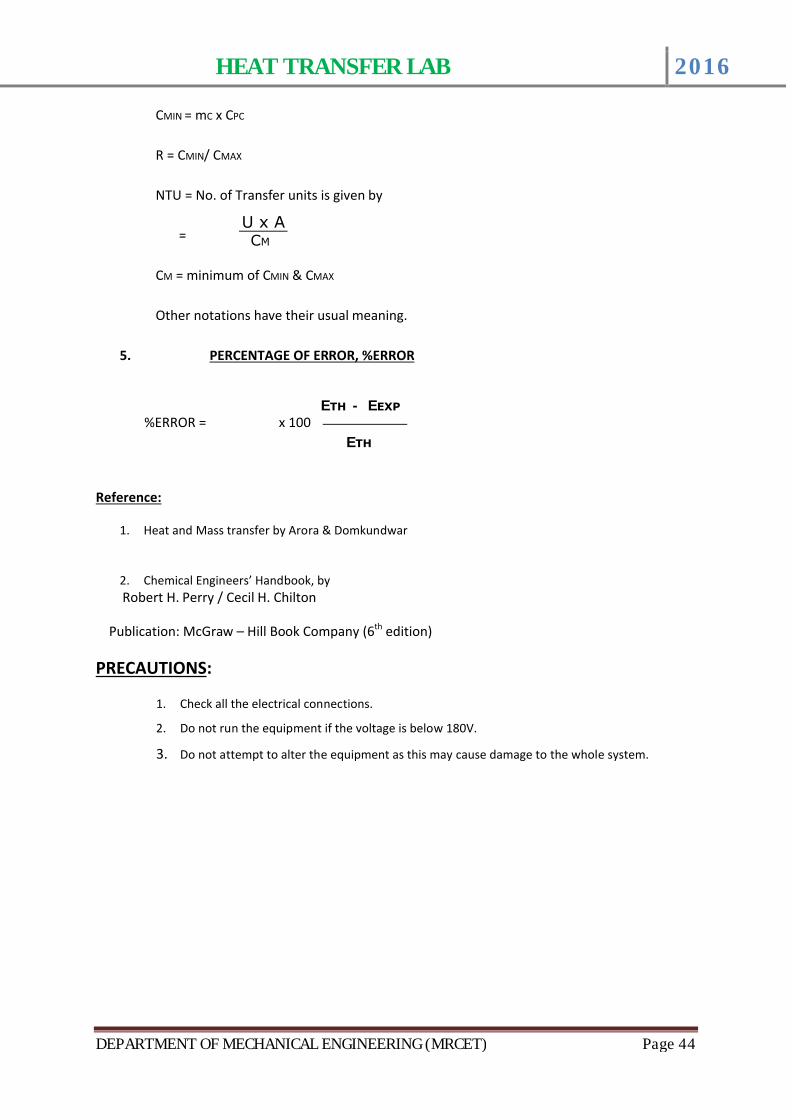
CMIN = mC x CPC
R = CMIN/ CMAX
NTU = No. of Transfer units is given by
=
CM = minimum of CMIN & CMAX
Other notations have their usual meaning.
5. PERCENTAGE OF ERROR, %ERROR
%ERROR = x 100
Reference:
1. Heat and Mass transfer by Arora & Domkundwar
2. Chemical Engineers’ Handbook, byRobert H. Perry / Cecil H. Chilton
Publication: McGraw – Hill Book Company (6th edition)
PRECAUTIONS:
1. Check all the electrical connections.
2. Do not run the equipment if the voltage is below 180V.
3. Do not attempt to alter the equipment as this may cause damage to the whole system.
U x ACM
ETH - EEXP
ETH
HEAT TRANSFER LAB 2016
DEPARTMENT OF MECHANICAL ENGINEERING (MRCET) Page 45
9. PIN-FIN APPARATUSINTRODUCTION:
A spine or pin-fin is an extended surface of cylindrical or conical shape used for increasing the heat
transfer rates from the surfaces, whenever it is not possible to increase the rate fo heat transfer
either by increasing heat transfer co-efficient or by increasing the temperature difference between
the surface and surrounding fluids.
The fins are commonly used on engine heads of scooter, motorcycles, as well as small capacity
compressors. The pin type fins are also used on the condenser of a domestic refrigerator.
DESCRIPTION OF THE APPARATUS:
The apparatus consists of
Pin type fin of dia 12mm and 150 mm long made of copper with suitable temperature points.
Heater of 250watts capacity.
Heater regulator to supply the regulated power input to the heater.
Digital Data logger is used to measure power input to the heater.
Thermocouples at suitable position to measure the surface temperatures of the fin.
Blower unit to blow air through the duct with orifice meter and acrylic manometer to
measure the air flow rate from the blower. A control valve is provided to regulate the air flow.
Control panel to house all the instrumentation.
With this the whole arrangement is mounted on an aesthetically
designed self-sustained MS powder coated frame with a separate control panel.
HEAT TRANSFER LAB 2016
DEPARTMENT OF MECHANICAL ENGINEERING (MRCET) Page 46
EXPERIMENTATION:
AIM:
1. To find out the temperature distribution along the given fin for constant base temperature under
natural and force flow conditions.
2. To find out effectiveness of the fin under both conditions.
PROCEDURE:
1. Switch on the MCB and then console on switch to activate the control panel.
2. Switch on the heater and regulate the power input using the heater regulator.
3. Switch on the blower unit and adjust the flow of air using gate valve of blower to a desired
difference in manometer (for forced flow only otherwise skip to step 4).
4. Wait for reasonable time to allow temperatures to reach steady state.
5. Measure the voltage, current and temperatures from T1 to T6 at known time interval.
6. Calculate the effectiveness & efficiency of the fin using the procedure given.
7. Repeat the experiment for different values of power input to the heater and blower air flow
rates.
PROCEDURE : COMPUTERIZED
TAKING READINGS – COMPUTERIZED
1. Switch on the panel.
2. Switch on the computer.
3. Open the “ HEAT TRANSFER Software” from the installed location a welcome screen will be
displayed
4. Follow the below steps to operate through software
5. Once the software is opened, the main screen will be displaced
6. Now, press “START” button, and the small screen will opened
7. Enter the parameters listed for particular test under study.
8. the software starts displaying the calculated values which can be cross verified based on the
formulae give after.
9. Select the Process Natural or Forced If you selected forced Switch on the Blower. U selected
Natural Air Flow is not Required .Switch of the Blower.
HEAT TRANSFER LAB 2016
DEPARTMENT OF MECHANICAL ENGINEERING (MRCET) Page 47
10. Switch on Blower And adjust the air Flow rate By using the Valve See the Air flow rate in
Indicator.
11. Switch on the heater and set the voltage (say 40V) using heater regulator.
12. Wait for sufficient time to allow temperature to reach steady values.
13. Repeat the experiment for different heat inputs and also for horizontal position with
different heat inputs.
14. Wait to attain the steady state.
15. Click the “store” button to store the value can be viewed anytime later.
16. After completion of the Experiment to press the stop button
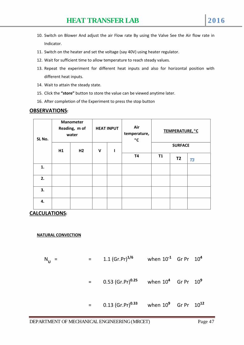
OBSERVATIONS:
SL No.
Manometer Reading, m of
waterHEAT INPUT Air
temperature, ∞C
TEMPERATURE, ∞C
H1 H2 V ISURFACE
T4 T1 T2 T3
1.
2.
3.
4.
CALCULATIONS:
NATURAL CONVECTION
NU = = 1.1 (Gr.Pr)1/6 when 10-1 Gr Pr 104
= 0.53 (Gr.Pr)0.25 when 104 Gr Pr 109
= 0.13 (Gr.Pr)0.33 when 109 Gr Pr 1012

HEAT TRANSFER LAB 2016
DEPARTMENT OF MECHANICAL ENGINEERING (MRCET) Page 48
Where,
Pr = Gr =
b = 1/(273+Tm)
where ,
Tm = mean effective temperature of the fin.
Ta = ambient temperature of the chamber.
All the properties of air should be taken at (Tm + Ta)/2 from the data hand book.
FORCED CONVECTION
NU = 0.615(Re)0.466when 40< Re > 4000
NU = 0.174(Re)0.168when 40 00 < Re > 40 x 103
rVD
Re = -----------
m
where ,D = inner diameter of the tube =
V m/s
Mass flow rate of air is calculated as follows:
= 0.62 x a x
where, a = , d= 0.020
H = (H1 ~ H2)x 1000 m of air column
Flow area is calculated as follows:
1.293
mCp
k
L3r2b (Tm -Ta)
2
HEAT TRANSFER LAB 2016
DEPARTMENT OF MECHANICAL ENGINEERING (MRCET) Page 49
= , D= 0.050
All the properties of air should be taken at (Tm + Ta)/2 from the data hand book.
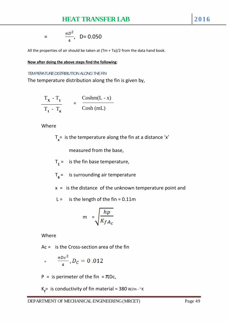
Now after doing the above steps find the following:
TEMPERATURE DISTRIBUTION ALONG THE FIN
The temperature distribution along the fin is given by,
=
Where
Tx= is the temperature along the fin at a distance ‘x’
measured from the base,
T1 = is the fin base temperature,
T6 = is surrounding air temperature
x = is the distance of the unknown temperature point and
L = is the length of the fin = 0.11m
m =
Where
Ac = is the Cross-section area of the fin
=
P = is perimeter of the fin = πDc,
Kf= is conductivity of fin material = 380 W/m - ∞K
TX
- T1
T1
- T6
Coshm(L - x)
Cosh (mL)
HEAT TRANSFER LAB 2016
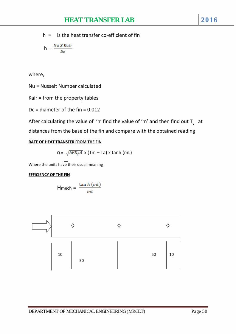
DEPARTMENT OF MECHANICAL ENGINEERING (MRCET) Page 50
h = is the heat transfer co-efficient of fin
h =
where,
Nu = Nusselt Number calculated
Kair = from the property tables
Dc = diameter of the fin = 0.012
After calculating the value of ‘h’ find the value of ‘m’ and then find out Tx at
distances from the base of the fin and compare with the obtained reading
RATE OF HEAT TRANSFER FROM THE FIN
Q = x (Tm – Ta) x tanh (mL)
Where the units have their usual meaning
EFFICIENCY OF THE FIN
Ηmech =
5050 1010
HEAT TRANSFER LAB 2016
DEPARTMENT OF MECHANICAL ENGINEERING (MRCET) Page 51
10.STEFAN BOLTZMAN’S APPARATUS INTRODUCTION:
The most commonly used relationship in radiation heat transfer is the Stefan Boltzman’s law which
relates the heat transfer rate to the temperatures of hat and cold surfaces.
q = s A ( T4H – T4C )
Where,
q = rate of heat transfer, watts
s = Stefan Boltzman’s constant = 5.669 x 10⁻⁸ watts/m² ∞K4
A = Surface area, m²
TH = Temperature of the hot body, ∞K
TC = Temperature of the cold body, ∞K
The above equation is applicable only to black bodies 9for example a piece of metal covered with
carbon black approximates this behavior) and is valid only for thermal radiation. Other types of
bodies (like a glossy painted surface or a polished metal plate) do not radiate as much energy as the
black body but still the total radiation emitted generally follow temperature proportionality.
DESCRIPTION OF THE APPARATUS:
The apparatus consists of
Copper hemispherical enclosure with insulation.
SS jacket to hold the hot water.
Over head water heater with quick release mechanism and the thermostat to generate and dump the hot water.Thermostat to supply the regulated power input to the heater.
Thermocouples at suitable position to measure the surface temperatures of the absorber
body.PID Indicator is used to measure the temperatures.Control panel to house all the
instrumentation.With this the whole arrangement is mounted on an aesthetically
HEAT TRANSFER LAB 2016
DEPARTMENT OF MECHANICAL ENGINEERING (MRCET) Page 52
designed self-sustained frame with a separate control panel.
EXPERIMENTATION:
AIM:
To determine the Stefan Boltman’s constant.PROCEDURE:
1. Fill water slowly into the overhead water heater.2. Switch on the supply mains and console.3. Switch on the heater and regulate the power input using the heater regulator. (say 60 – 85
∞C)
4. After water attains the maximum temperature, open the valve of the heater and dump to
the enclosure jacket.
5. Wait for about few seconds to allow hemispherical enclosure to attain uniform temperature
– the chamber will soon reach the equilibrium. Note the enclosure temperature.
6. Insert the Test specimen with the sleeve into its position and record the temperature at
different instants of time using the stop watch.
7. Plot the variation of specimen temperature with time and get the slope of temperature
versus time variation at the time t = 0 sec
8. Calculate the Stefan Boltzman’s constant using the equations provided.
9. Repeat the experiment 3 to 4 times and calculate the average value to obtain the better
results.
PROCEDURE : COMPUTERIZED
TAKING READINGS – COMPUTERIZED
1. switch on the panel.
2. Switch on the computer.
3. Open the “ HEAT TRANSFER Software” from the installed location a welcome screen will be displayed
4. Follow the below steps to operate through software
5. Once the software is opened, the main screen will be displaced On the main screen press “PORT”
button and select the USB port connected,
6. Now, press “START” button, and the small screen will opened
7. Enter the parameters listed for particular test under study.
8. Now, set the temp by using thermostat regulator to known valve.
HEAT TRANSFER LAB 2016
DEPARTMENT OF MECHANICAL ENGINEERING (MRCET) Page 53
9. Now press “START BUTTON” on the screen so the software automatically starts recording the temperatures and other values.
10. Switch on the heater and regulate the power input using the heater regulator. (say 60 – 85 ∞C)
11. After water attains the maximum temperature, open the valve of the heater and dump to the
enclosure jacket.
12. Wait for about few seconds to allow hemispherical enclosure to attain uniform temperature – the
chamber will soon reach the equilibrium. Note the enclosure temperature.
13. Also, the software starts displaying the calculated values which can be cross verified based on the formulae give there after.
14. Enter the STORE BUTTON to store the values.
15. Press report button to see the stored values
16. finally thermostat you kept at 0 *C
OBSERVATIONS:
Enclosure Temperature, Te =
Initial Temperature of the specimen, Ts =
Time, tSpecimen
Temperature, Ts
5
10
15
20
25
30
CALCULATIONS:
STEFAN BOLTMAN’S CONSTANT IS CALCULATED USING THE RELATION:
s =
Where, m = mass of the test specimen = 0.0047Kg
Cp = Specific heat of the specimen = 410 J/Kg ∞C
HEAT TRANSFER LAB 2016
DEPARTMENT OF MECHANICAL ENGINEERING (MRCET) Page 54
Te = Enclosure temperature, ∞K
TS = Initial temperature of the specimen, ∞K
(dTa/dt) = calculated from graph.
AD = Surface area of the test specimen
= pd²/4
where d = 0.015m
RESULT:
Stefan Boltzman’s constant is _______________
Reference:
1. Heat and Mass transfer by Arora & Domkundwar
2. Chemical Engineers’ Handbook, byRobert H. Perry / Cecil H. Chilton
Publication: McGraw – Hill Book Company (6th edition)
PRECAUTIONS:
1. Check all the electrical connections.
2. Do not run the equipment if the voltage is below 180V.
3. Do not switch on the heater without water in the overhead tank.
4. Do not turn the heater regulator to the maximum as soon as the equipment is started.
5. Do not attempt to alter the equipment as this may cause damage to the whole system.
HEAT TRANSFER LAB 2016
DEPARTMENT OF MECHANICAL ENGINEERING (MRCET) Page 55
11.THERMAL CONDUCTIVITY OF CONCENTRIC SPHERE
INTRODUCTION:
Thermal conductivity is the physical property of material denoting the ease with a particular substance can accomplish the transmission of thermal energy by molecular motion.
Thermal conductivity of a material is found, to depend on the chemical composition of the
substances of which it is a composed, the phase (i.e. gas, liquid or solid) in which its crystalline
structure if a solid, the temperature & pressure to which it is subjected and whether or not it is
homogeneous material.
Thermal energy in solids may be conducted in two modes. They are:
ÿ LATTICE VIBRATION:
ÿ TRANSPORT BY FREE ELECTRONS.
In good electrical conductors a rather large number of free electrons move about in a lattice
structure of the material. Just as these electrons may transport may transport electric charge, they
may also carry thermal energy from a high temperature region to low temperature region. In fact,
these electrons are frequently referred as the electron gas. Energy may also be transmitted as
vibrational energy in the lattice structure of the material. In general, however, this latter mode of
energy transfer is not as large as the electron transport and it is for this reason that good electrical
conductors are almost always good heat conductors, for eg: ALUMINIUM, COPPER & SILVER.
With the increase in temperature, however the increased lattice vibrations come in the way
of electron transport by free electrons and for most of the pure metals the thermal conductivity
decreases with the increase in the temperature.
DESCRIPTION OF THE APPARATUS:
The apparatus consists of the COPPER sphere of 150mm dia and 250mm dia concentrically placed.
Heat is provided by means of oil bath heater arrangement. Thermocouples are provided at the
suitable points to measure the surface and inner temperatures. Proper insulation is provided to
minimize the heat loss. The temperature is shown by means of the DATA LOGGER on the control
panel, which also consists of heater regulator and other accessories instrumentation having good
aesthetic looks and safe design.
HEAT TRANSFER LAB 2016
DEPARTMENT OF MECHANICAL ENGINEERING (MRCET) Page 56
EXPERIMENTATION:
AIM:
To determine the THERMAL CONDUCTIVITY of given concentric sphere.
PROCEDURE:
1. Give necessary electrical and water connections to the instrument.
2. Switch on the MCB and console ON to activate the control panel.
3. Give input to the heater by slowly rotating the heater regulator.
4. Note the temperature at different points, when steady state is reached.
5. Repeat the experiment for different heater input.
6. After the experiment is over, switch off the electrical connections.
PROCEDURE : COMPUTERIZED
TAKING READINGS – COMPUTERIZED
1. Switch on the panel.
2. Switch on the computer.
3. Open the “ HEAT TRANSFER Software” from the installed location a welcome screen will be
displayed
4. Follow the below steps to operate through software
5. Once the software is opened, the main screen will be displaced
6. Now, press “START” button, and the small screen will opened
7. Enter the parameters listed for particular test under study.
8. the software starts displaying the calculated values which can be cross verified based on the formulae give after.
9. Before switch on the Heater Please check the Oil.
10. Switch on the heater and set the voltage (say 40V) using heater regulator.
11. Wait for sufficient time to allow temperature to reach steady values.
12. Repeat the experiment for different heat inputs and different heat inputs.
13. Wait to attain the steady state.
14. Click the “store” button to store the value can be viewed anytime later.
15. After completion of the Experiment to press the stop button
HEAT TRANSFER LAB 2016
DEPARTMENT OF MECHANICAL ENGINEERING (MRCET) Page 57
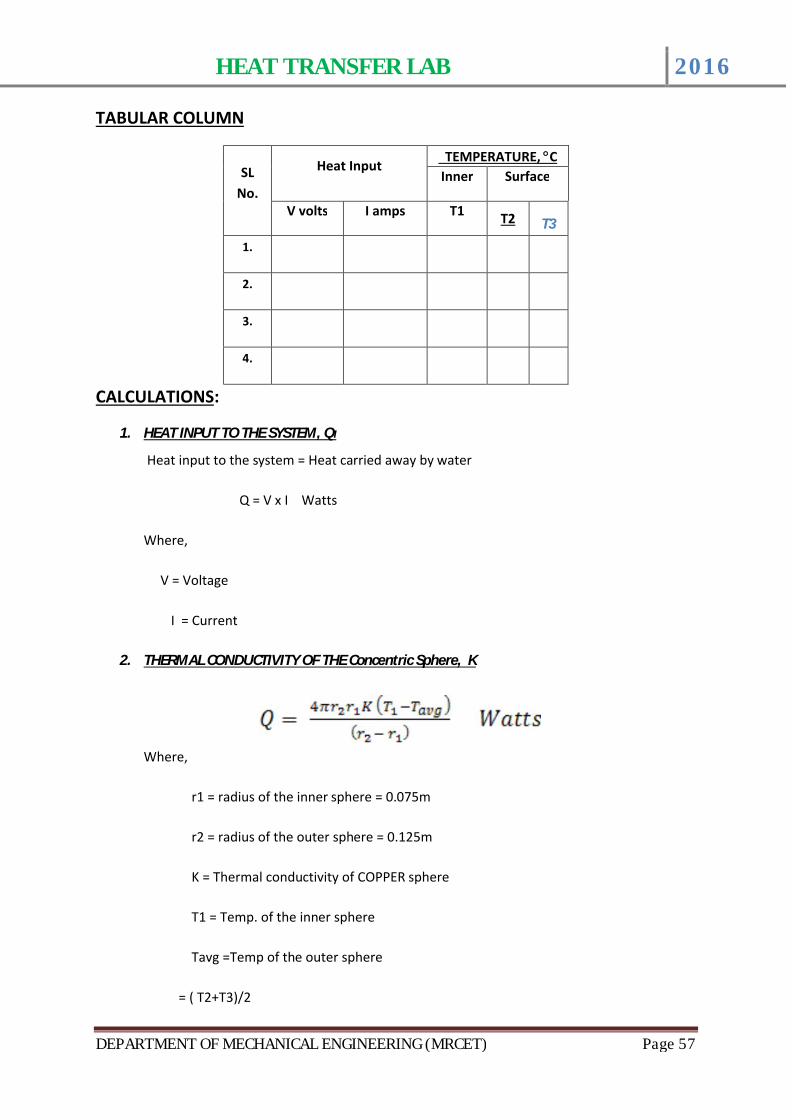
TABULAR COLUMN
SL No.
Heat InputTEMPERATURE, ∞C
Inner Surface
V volts I amps T1 T2 T3
1.
2.
3.
4.
CALCULATIONS:
1. HEAT INPUT TO THE SYSTEM, QI
Heat input to the system = Heat carried away by water
Q = V x I Watts
Where,
V = Voltage
I = Current
2. THERMAL CONDUCTIVITY OF THE Concentric Sphere, K
Where,
r1 = radius of the inner sphere = 0.075m
r2 = radius of the outer sphere = 0.125m
K = Thermal conductivity of COPPER sphere
T1 = Temp. of the inner sphere
Tavg =Temp of the outer sphere
= ( T2+T3)/2
HEAT TRANSFER LAB 2016
DEPARTMENT OF MECHANICAL ENGINEERING (MRCET) Page 58
PRECAUTIONS:
1. Input should be given very slowly.
2. Do not run the equipment if the voltage is below 180V.
3. Check all the electrical connections before running.
4. Before starting and after finishing the experiment the heater controller should be in off position.
5. Do not attempt to alter the equipment as this may cause damage to the whole system.
Reference:
1. PROCESS HEAT TRANSFER, by2. Wareh L. McCabe3. Julian C. Smith4. Peter Harioth 5. Publication: McGraw Hill (6th edition)6. Heat and Mass transfer by Arora & Domkundwar7. Chemical Engineers’ Handbook, by8. Robert H. Perry / Cecil H. Chilton
Publication: McGraw – Hill Book Company (6th edition)
HEAT TRANSFER LAB 2016
DEPARTMENT OF MECHANICAL ENGINEERING (MRCET) Page 59
12.THERMAL CONDUCTIVITY OF METAL ROD
INTRODUCTION:
Thermal conductivity is the physical property of material denoting the ease with a particular substance can accomplish the transmission of thermal energy by molecular motion.
Thermal conductivity of a material is found, to depend on the chemical composition of the substances of which it is a composed, the phase (i.e. gas, liquid or solid) in which its crystalline structure if a solid, the temperature & pressure to which it is subjected and whether or not it is homogeneous material.
Thermal energy in solids may be conducted in two modes. They are:
ÿ LATTICE VIBRATION: ÿ TRANSPORT BY FREE ELECTRONS.In good electrical conductors a rather large number of free electrons move about in a lattice
structure of the material. Just as these electrons may transport may transport electric charge, they
may also carry thermal energy from a high temperature region to low temperature region. In fact,
these electrons are frequently referred as the electron gas. Energy may also be transmitted as
vibrational energy in the lattice structure of the material. In general, however, this latter mode of
energy transfer is not as large as the electron transport and it is for this reason that good electrical
conductors are almost always good heat conductors, for eg: ALUMINIUM, COPPER & SILVER.
With the increase in temperature, however the increased lattice vibrations come in the way
of electron transport by free electrons and for most of the pure metals the thermal conductivity
decreases with the increase in the temperature.
DESCRIPTION OF THE APPARATUS:
The apparatus consists of the COPPER rod of 200mm test section. Heat is provided by means of
band heater at one end and released through water jacket arrangement. Thermocouples are
provided at the suitable points to measure the surface and water temperatures. Proper insulation is
provided to minimize the heat loss. The temperature is shown by means of the Data logger on the
control panel, which also consists of heater regulator and other accessories instrumentation having
good aesthetic looks and safe design.
HEAT TRANSFER LAB 2016
DEPARTMENT OF MECHANICAL ENGINEERING (MRCET) Page 60
EXPERIMENTATION:
AIM:
To determine the THERMAL CONDUCTIVITY of given metal rod.
PROCEDURE:
1. Give necessary electrical and water connections to the instrument.
2. Switch on the MCB and console ON to activate the control panel.
3. Give input to the heater by slowly rotating the heater regulator.
4. Start the cooling water supply through the water jacket (make sure not to exceed 3 lpm).
5. Note the temperature at different points, when steady state is reached.
6. Repeat the experiment for different heater input.
7. After the experiment is over, switch off the electrical connections, allow the water to flow for some
time in the water jacket and then stop it.
PROCEDURE : COMPUTERIZED
TAKING READINGS – COMPUTERIZED
1. Turn on the computer switch on the panel.
2. Switch on the computer.
3. Open the “ HEAT TRANSFER Software” from the installed location a welcome screen will be
displayed
4. Follow the below steps to operate through software
5. Once the software is opened, the main screen will be displaced
6. Now, press “START” button, and the small screen will opened
7. Enter the parameters listed for particular test under study.
8. the software starts displaying the calculated values which can be cross verified based on the
formulae give after.
9. Give input to the heater by slowly rotating the heater regulator.
10. Start the cooling water supply through the water jacket (make sure not to exceed 3 lpm).
11. Click the “store” button to store the value can be viewed anytime later.
12. After completion of the Experiment to press the stop button.
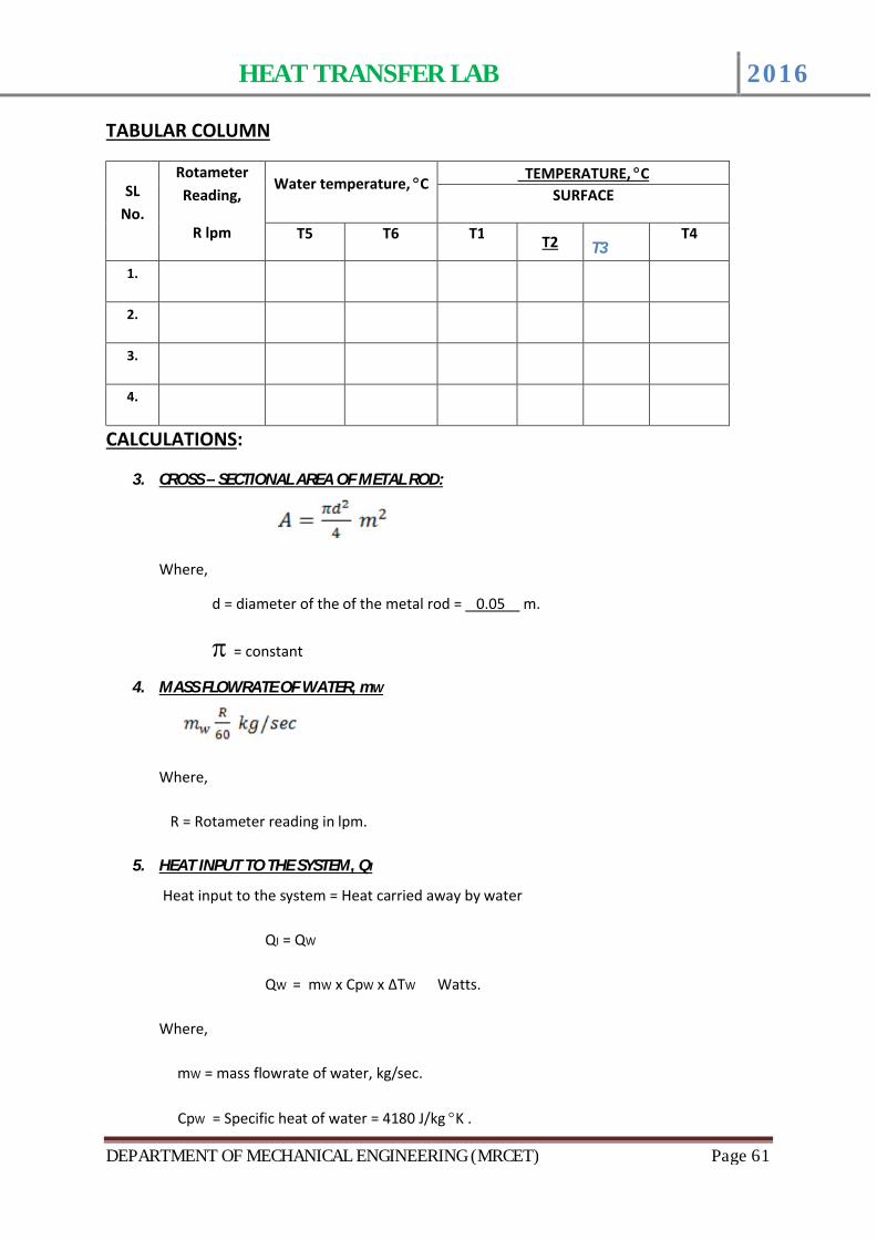
HEAT TRANSFER LAB 2016
DEPARTMENT OF MECHANICAL ENGINEERING (MRCET) Page 61
TABULAR COLUMN
SL No.
Rotameter Reading,
R lpm
Water temperature, ∞CTEMPERATURE, ∞C
SURFACE
T5 T6 T1 T2 T3T4
1.
2.
3.
4.
CALCULATIONS:
3. CROSS – SECTIONAL AREA OF METAL ROD:
Where,
d = diameter of the of the metal rod = 0.05 m.
p = constant
4. MASS FLOWRATE OF WATER, mW
Where,
R = Rotameter reading in lpm.
5. HEAT INPUT TO THE SYSTEM, QI
Heat input to the system = Heat carried away by water
QI = QW
QW = mW x CpW x ΔTW Watts.
Where,
mW = mass flowrate of water, kg/sec.
CpW = Specific heat of water = 4180 J/kg ∞K .
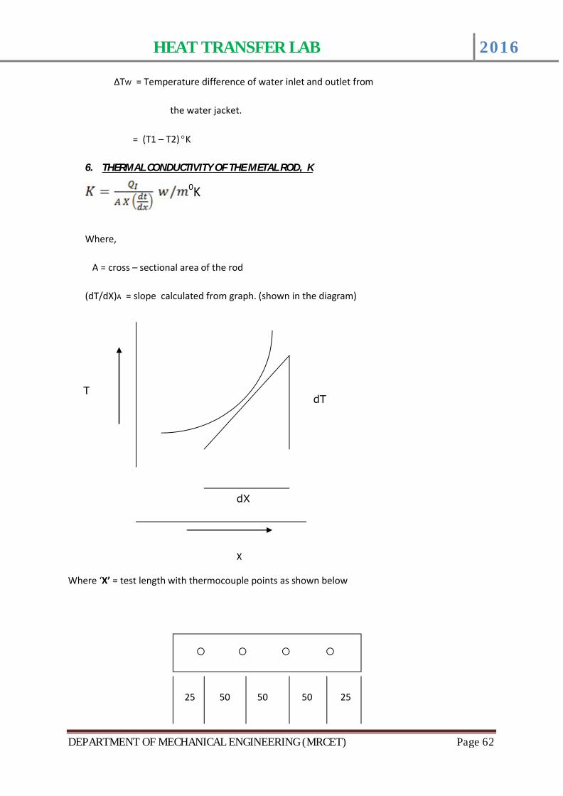
HEAT TRANSFER LAB 2016
DEPARTMENT OF MECHANICAL ENGINEERING (MRCET) Page 62
ΔTW = Temperature difference of water inlet and outlet from
the water jacket.
= (T1 – T2) ∞K
6. THERMAL CONDUCTIVITY OF THE METAL ROD, K
0K
Where,
A = cross – sectional area of the rod
(dT/dX)A = slope calculated from graph. (shown in the diagram)
Where ‘X’ = test length with thermocouple points as shown below
T
X
dT
dX
50 50 50 2525
HEAT TRANSFER LAB 2016
DEPARTMENT OF MECHANICAL ENGINEERING (MRCET) Page 63
PRECAUTIONS:
1. Do not give heater input without the supply of water.
2. Input should be given very slowly.
3. Run the water in the jacket for about 5 min after the experiment.
4. Do not run the equipment if the voltage is below 180V.
5. Check all the electrical connections before running.
6. Before starting and after finishing the experiment the heater controller should be in off position.
7. Do not attempt to alter the equipment as this may cause damage to the whole system.
Reference:
1 PROCESS HEAT TRANSFER, byWareh L. McCabe
Julian C. Smith
Peter Harioth
Publication: McGraw Hill (6th edition)
2 Heat and Mass transfer by Arora & Domkundwar3 Chemical Engineers’ Handbook, by
Robert H. Perry / Cecil H. Chilton
Publication: McGraw – Hill Book Company (6th edition)
HEAT TRANSFER LAB 2016
DEPARTMENT OF MECHANICAL ENGINEERING (MRCET) Page 64
13.TRANSIENT HEAT CONDUCTION APPARATUS
INTRODUCTION:
When a body is subjected to heating or cooling, irrespective of the material it
requires certain time to attain steady state. Hence the other way of expressing is that the
unsteady process will occur till it attains the steady process. In unsteady process the
temperature will change with respect to time. Although, temperature of the body is
generally expressed as the function of 3 different axis and time, it is not easy to solve.
Unsteady state heating or cooling can be categorized as:
ÿ PERIODIC HEAT FLOW : where the temperature within the
system undergoes periodic changes which may be regular or
irregular.
ÿ NON – PERIODIC HEAT FLOW : where the temperature at
any point within the system changes non – linearly with
respect to time.
Unsteady state heat flow is very common in all heating or cooling problems at the
beginning of the system. Hardening by qrenching, cooling of IC engine cylinders, and heating
of boiler tubes are common examples of unsteady state heat flow.
2. DESCRIPTION OF APPARATUS:
ÿ The apparatus consists of a specially designed Stainless Steel Tank with heater arrangement.
ÿ An ALUMINIUM sphere is provided to study the experiment with the stand to place in the
heater tank.
ÿ Heater regulator with Thermostat to supply the regulated power input to the heater
and to set the temperature.
ÿ Thermocouples at suitable position to measure the temperatures.
ÿ Digital data logger used to measure the temperatures.
ÿ The whole arrangement is mounted on an Aesthetically designed sturdy frame made of
NOVAPAN Board with all the provisions for holding the tanks and accessories.
HEAT TRANSFER LAB 2016
DEPARTMENT OF MECHANICAL ENGINEERING (MRCET) Page 65
3. EXPERIMENTATION:
AIM:ÿ To determine heat transfer coefficient and instantaneous heat transfer rate for
transient heat conduction and draw the graph of temperature variation with
time
PROCEDURE : MANUAL1. Take the fluid (water or oil) in the tank.
2. Heat the fluid to the required temperature say 70oC in case of water and more than
100 oC in case of oil.
3. Note down the initial temperature of sphere and hot fluid.
4. Immerse the sphere in hot fluid bath for heating.
5. Note down the surface temperature of the sphere at every 10 seconds till it attains
fluid temperature.
6. Take out the sphere from hot fluid and cool it in atmospheric air.
7. Repeat the experiment for different temperatures of fluid.
PROCEDURE : COMPUTERIZEDTAKING READINGS – COMPUTERIZED
1. switch on the panel.
2. Switch on the computer.
3. Open the “ HEAT TRANSFER Software” from the installed location a welcome screen
will be displayed
4. Follow the below steps to operate through software
5. Once the software is opened, the main screen will be displaced On the main screen
press “PORT” button and select the USB port connected,
6. Now, press “START” button, and the small screen will opened
7. Enter the parameters listed for particular test under study.
8. Now, set the temp by using thermostat regulator to known valve.
9. Now press “START BUTTON” on the screen so the software automatically starts recording the temperatures and other values.
10. Also, the software starts displaying the calculated values which can be cross verified based on the formulae give there after.
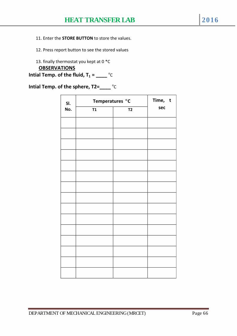
HEAT TRANSFER LAB 2016
DEPARTMENT OF MECHANICAL ENGINEERING (MRCET) Page 66
11. Enter the STORE BUTTON to store the values.
12. Press report button to see the stored values
13. finally thermostat you kept at 0 *COBSERVATIONS
Intial Temp. of the fluid, T1 = ____ oC
Intial Temp. of the sphere, T2=____ oC
Sl. No.
Temperatures ∞C Time, t secT1 T2
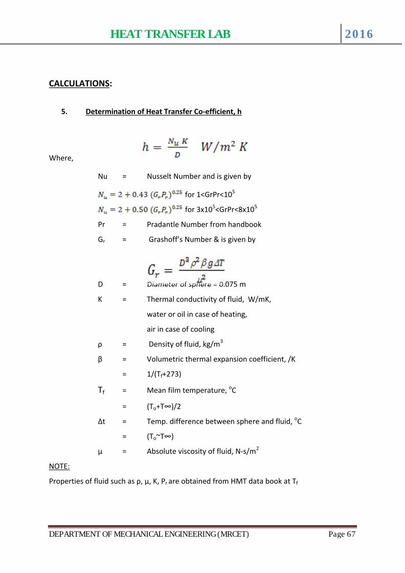
HEAT TRANSFER LAB 2016
DEPARTMENT OF MECHANICAL ENGINEERING (MRCET) Page 67
CALCULATIONS:
5. Determination of Heat Transfer Co-efficient, h
Where,
Nu = Nusselt Number and is given by
for 1<GrPr<105
for 3x10⁵<GrPr<8x10⁵
Pr = Pradantle Number from handbook
Gr = Grashoff’s Number & is given by
D =
K = Thermal conductivity of fluid, W/mK,
water or oil in case of heating,
air in case of cooling
ρ = Density of fluid, kg/m3
β = Volumetric thermal expansion coefficient, /K
= 1/(Tf+273)
Tf = Mean film temperature, oC
= (To+T∞)/2
∆t = Temp. difference between sphere and fluid, oC
= (To~T∞)
µ = Absolute viscosity of fluid, N-s/m2
NOTE:
Properties of fluid such as ρ, µ, K, Pr are obtained from HMT data book at Tf
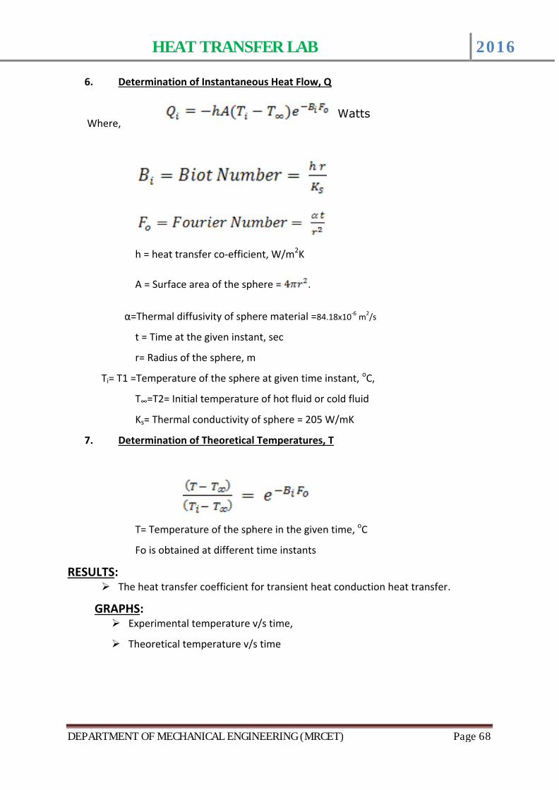
HEAT TRANSFER LAB 2016
DEPARTMENT OF MECHANICAL ENGINEERING (MRCET) Page 68
6. Determination of Instantaneous Heat Flow, Q
Where,
h = heat transfer co-efficient, W/m2K
A = Surface area of the sphere = .
α=Thermal diffusivity of sphere material =84.18x10⁻⁶ m2/s
t = Time at the given instant, sec
r= Radius of the sphere, m
Ti= T1 =Temperature of the sphere at given time instant, oC,
T∞=T2= Initial temperature of hot fluid or cold fluid
Ks= Thermal conductivity of sphere = 205 W/mK
7. Determination of Theoretical Temperatures, T
T= Temperature of the sphere in the given time, oC
Fo is obtained at different time instants
RESULTS:ÿ The heat transfer coefficient for transient heat conduction heat transfer.
GRAPHS:ÿ Experimental temperature v/s time,
ÿ Theoretical temperature v/s time
Watts
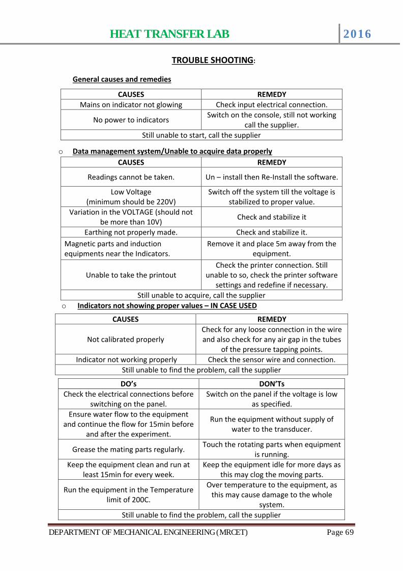
HEAT TRANSFER LAB 2016
DEPARTMENT OF MECHANICAL ENGINEERING (MRCET) Page 69
TROUBLE SHOOTING:
o General causes and remedies
CAUSES REMEDYMains on indicator not glowing Check input electrical connection.
No power to indicators Switch on the console, still not working call the supplier.
Still unable to start, call the supplier
o Data management system/Unable to acquire data properlyCAUSES REMEDY
Readings cannot be taken. Un – install then Re-Install the software.
Low Voltage (minimum should be 220V)
Switch off the system till the voltage is stabilized to proper value.
Variation in the VOLTAGE (should not be more than 10V) Check and stabilize it
Earthing not properly made. Check and stabilize it.Magnetic parts and induction equipments near the Indicators.
Remove it and place 5m away from the equipment.
Unable to take the printoutCheck the printer connection. Still
unable to so, check the printer software settings and redefine if necessary.
Still unable to acquire, call the suppliero Indicators not showing proper values – IN CASE USED
CAUSES REMEDY
Not calibrated properlyCheck for any loose connection in the wire and also check for any air gap in the tubes
of the pressure tapping points.Indicator not working properly Check the sensor wire and connection.
Still unable to find the problem, call the supplier
DO’s DON’TsCheck the electrical connections before
switching on the panel.Switch on the panel if the voltage is low
as specified.Ensure water flow to the equipment
and continue the flow for 15min before and after the experiment.
Run the equipment without supply of water to the transducer.
Grease the mating parts regularly. Touch the rotating parts when equipment is running.
Keep the equipment clean and run at least 15min for every week.
Keep the equipment idle for more days as this may clog the moving parts.
Run the equipment in the Temperature limit of 200C.
Over temperature to the equipment, as this may cause damage to the whole
system.Still unable to find the problem, call the supplier
HEAT TRANSFER LAB 2016
DEPARTMENT OF MECHANICAL ENGINEERING (MRCET) Page 70
LIMITATIONS & PRECAUTIONS
1. Maximum Load is limited to 70∞C.
2. This is a general equipment for study in undergraduate level, for consideration of
higher level studies you can add any extra parameter required. For adding the
parameters call the supplier.
3. Don’t run the equipment if the voltage is less than 180V.
4. 230V, 1ph with neutral and proper earthing to be provided.
5. Don’t alter the equipment without the supervision of the supplier.
Reference:
1 Heat and Mass transfer by Arora & Domkundwar2 Chemical Engineers’ Handbook, by
Robert H. Perry / Cecil H. Chilton
Publication: McGraw – Hill Book Company (6th edition)
HEAT TRANSFER LAB 2016
DEPARTMENT OF MECHANICAL ENGINEERING (MRCET) Page 71
14.CONDENSATION APPARATUSINTRODUCTION:
Condensation is the process of change of state free vapour to liquid.
Condensation occurs on a surface when the vapour saturation
temperature is higher than the temperature of surface. The temperature
of the condensate so formed will be less than the saturation temperature
of the vapour and becomes sub-cooled. More vapour starts condensing on
the exposed surface or on the previous condensate, since the
temperature of the previous condensate is lower.
The phenomenon of condensation heat transfer is more complex,
which involves change of phase and additional characteristics / variables
that control the condensation process.
There are two basic types of condensation - Film Condensation and
Dropwise Condensation.
a) Film Condensation :
When the condensate tends to “wet” the surface, then it is called
“film condensation”. In this process, the liquid condensate distributes
itself as a continuous thin film on the cooled surface. This happens when
the surface tension between the liquid and the solid material is sufficiently
small for example, condensation of steam on a clean metallic surface,
when the surface is clean and grease / oil free.
In film condensation, heat transfer from the vapour to the
cooling surface takes place through the condensate film formed on the
surface. As the new condensate formed joins the film existing on the
surface, the film thickness increases. The heat is transferred from the
vapour to the condensate by convection and further from condensate to
the surface by conduction. This combined mode of heat transfer by
conduction and convection reduce the rate of heat transfer in film
HEAT TRANSFER LAB 2016
DEPARTMENT OF MECHANICAL ENGINEERING (MRCET) Page 72
condensation process. Hence, the rate of heat transfer is lower in film
condensation (as compared to dropwise condensation).
b) Dropwise Condensation :
When the condensate does not wet the surface, it forms the
droplets on the surface, it is known as “dropwise condensation”. When the
surface tension is large, the condensate coalesces into a multitude of
droplets of different sizes. With time, each droplet grows as more vapour
condenses on its exposed surface. The formation of each droplet is
initiated at a point of surface imperfection (pit, scratch, etc.) and such
sites are called “nucleation sites”. At some time, the tangential pull of
gravity, or sheer force exerted by the vapour stream, dislodges the
droplet and carries it downstream. The moving droplet devours the
smaller droplets in its path, thereby creating a clean trail ready for the
generation of new droplets of smaller sizes. This surface renewal process
occurs periodically as the droplets accumulate and grow in size. Since the
condensation rate is the highest in the absence of condensate on the
surface, the periodic cleaning performed by the large drops renews finite
size regions of the surface for the restart of the condensation. This
surface renewal process is the main reason why dropwise condensation is
a highly effective heat transfer mechanism. The heat transfer coefficient is
roughly ten times greater than the corresponding condensation in the
form of thin film.
In the design of condensers, whose function is to cool a vapour
stream and to convert it into liquid, there is a great advantage to promote
the breakup of the condensate into droplets. This can be achieved by :
a) Coating the solid surface with an organic substance like
wax, oil, oleic acid, etc.
b) Injecting non-wetting chemicals into the vapour, which
get deposited on the surface of the condenser.
HEAT TRANSFER LAB 2016
DEPARTMENT OF MECHANICAL ENGINEERING (MRCET) Page 73
c) Coating the surface with a polymer of low surface energy
like teflon, silicone, etc. or with a noble metal like gold,
silver, etc.
The mechanism of dropwise condensation is complex because
of its intermittent time dependent character, effect of surface tension
(due to drop size and shape) and the uncertainty associated with the
location of nucleation sites and the time when the largest droplet will start
its downstream movement. Hence, a unifying theory of dropwise
condensation has not been developed.
DESCRIPTION OF THE APPARATUS:
The apparatus consists of
Heat exchanger tube made of copper which is placed inside the
GLASS CHAMBER of dimension j100 x 200mm.
Steam Generator with necessary fittings and accessories to generate and supply the steam.Rotameter to directly measure the flowrate of the water into the
condensate tube.
Thermocouples at suitable position to measure the temperatures
of body and the air.
Digital Temperature Indicator with channel selector to measure
the temperatures.
Control panel to house all the instrumentation.
With this the whole arrangement is mounted on an aesthetically designed self-sustained MS powder coated frame with a separate control
panel.
HEAT TRANSFER LAB 2016
DEPARTMENT OF MECHANICAL ENGINEERING (MRCET) Page 74
EXPERIMENTATION:
AIM:
ÿ To determine overall heat transfer coefficient (UO)
ÿ To determine steam side film coefficient (hS)
ÿ To determine cold fluid heat transfer coefficient (hI)
ÿ To draw Wilson’s plot and hence calculate the value of hI
theoretical from graph.(optional)
PROCEDURE:
1. Fill water slowly into the water tank and steam generator.
2. Switch on the supply mains and console.
3. Switch on the heater of steam generator to generate the steam.
4. Once the steam is generated follow the steps below.
5. Open the inlet valve and allow the cold fluid to flow through the
condenser.
6. Adjust the flowrate of cold fluid to minimum.
7. *Open the steam inlet valve and keep steam pressure constant (say
0.2kg/cm²) throughout the experiment.
8. After cold fluid temperature becomes steady state, note down the inlet
temperature, out let temperature and flowrate of cold fluid and also
note down the volume of condensate collected at the given time
interval(say 1min).
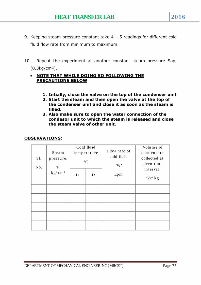
HEAT TRANSFER LAB 2016
DEPARTMENT OF MECHANICAL ENGINEERING (MRCET) Page 75
9. Keeping steam pressure constant take 4 – 5 readings for different cold
fluid flow rate from minimum to maximum.
10. Repeat the experiment at another constant steam pressure Say,
(0.3kg/cm²).
∑ NOTE THAT WHILE DOING SO FOLLOWING THE PRECAUTIONS BELOW
1. Intially, close the valve on the top of the condenser unit 2. Start the steam and then open the valve at the top of
the condenser unit and close it as soon as the steam is filled.
3. Also make sure to open the water connection of the condesor unit to which the steam is released and close the steam valve of other unit.
OBSERVATIONS:
Sl.
No.
Steam pressure.
‘P’ kg/cm²
Cold fluid temperature
∞C
Flow rate of cold fluid
‘W’
Lpm
Volume of condensate collected at given timeinterval,
‘Vc’ kgt1 t2
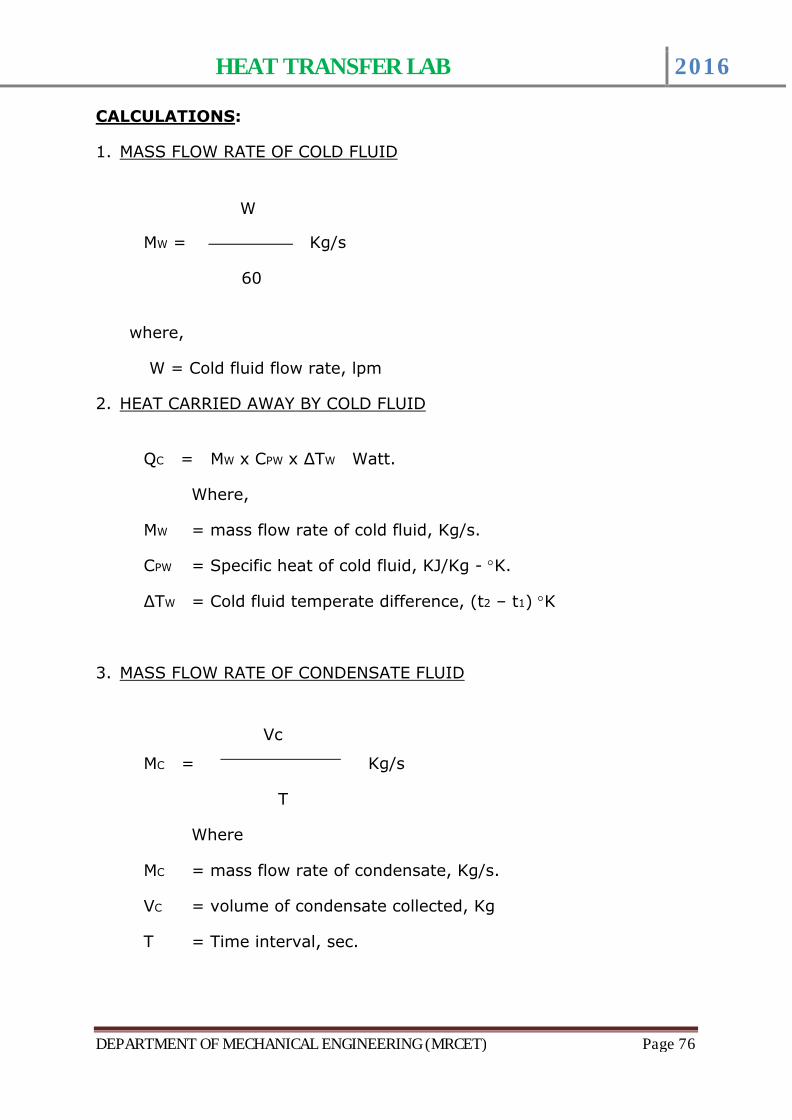
HEAT TRANSFER LAB 2016
DEPARTMENT OF MECHANICAL ENGINEERING (MRCET) Page 76
CALCULATIONS:
1. MASS FLOW RATE OF COLD FLUID
MW = Kg/s
60
where,
W = Cold fluid flow rate, lpm
2. HEAT CARRIED AWAY BY COLD FLUID
QC = MW x CPW x ΔTW Watt.
Where,
MW = mass flow rate of cold fluid, Kg/s.
CPW = Specific heat of cold fluid, KJ/Kg - ∞K.
ΔTW = Cold fluid temperate difference, (t2 – t1) ∞K
3. MASS FLOW RATE OF CONDENSATE FLUID
MC = Kg/s
T
Where
MC = mass flow rate of condensate, Kg/s.
VC = volume of condensate collected, Kg
T = Time interval, sec.
W
Vc
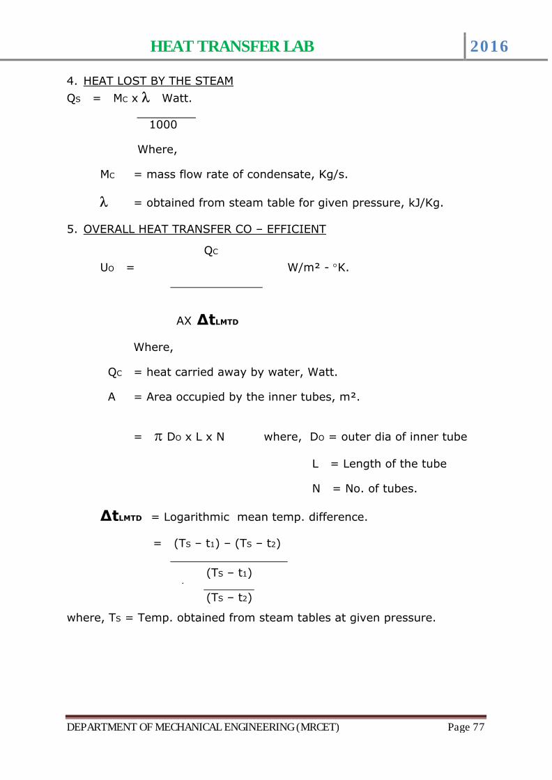
HEAT TRANSFER LAB 2016
DEPARTMENT OF MECHANICAL ENGINEERING (MRCET) Page 77
(TS – t1)
(TS – t2)Ln
4. HEAT LOST BY THE STEAM
QS = MC x l Watt.
1000
Where,
MC = mass flow rate of condensate, Kg/s.
l = obtained from steam table for given pressure, kJ/Kg.
5. OVERALL HEAT TRANSFER CO – EFFICIENT
UO = W/m² - ∞K.
AX ΔtLMTD
Where,
QC = heat carried away by water, Watt.
A = Area occupied by the inner tubes, m².
= p DO x L x N where, DO = outer dia of inner tube
L = Length of the tube
N = No. of tubes.
ΔtLMTD = Logarithmic mean temp. difference.
= (TS – t1) – (TS – t2)
where, TS = Temp. obtained from steam tables at given pressure.
QC
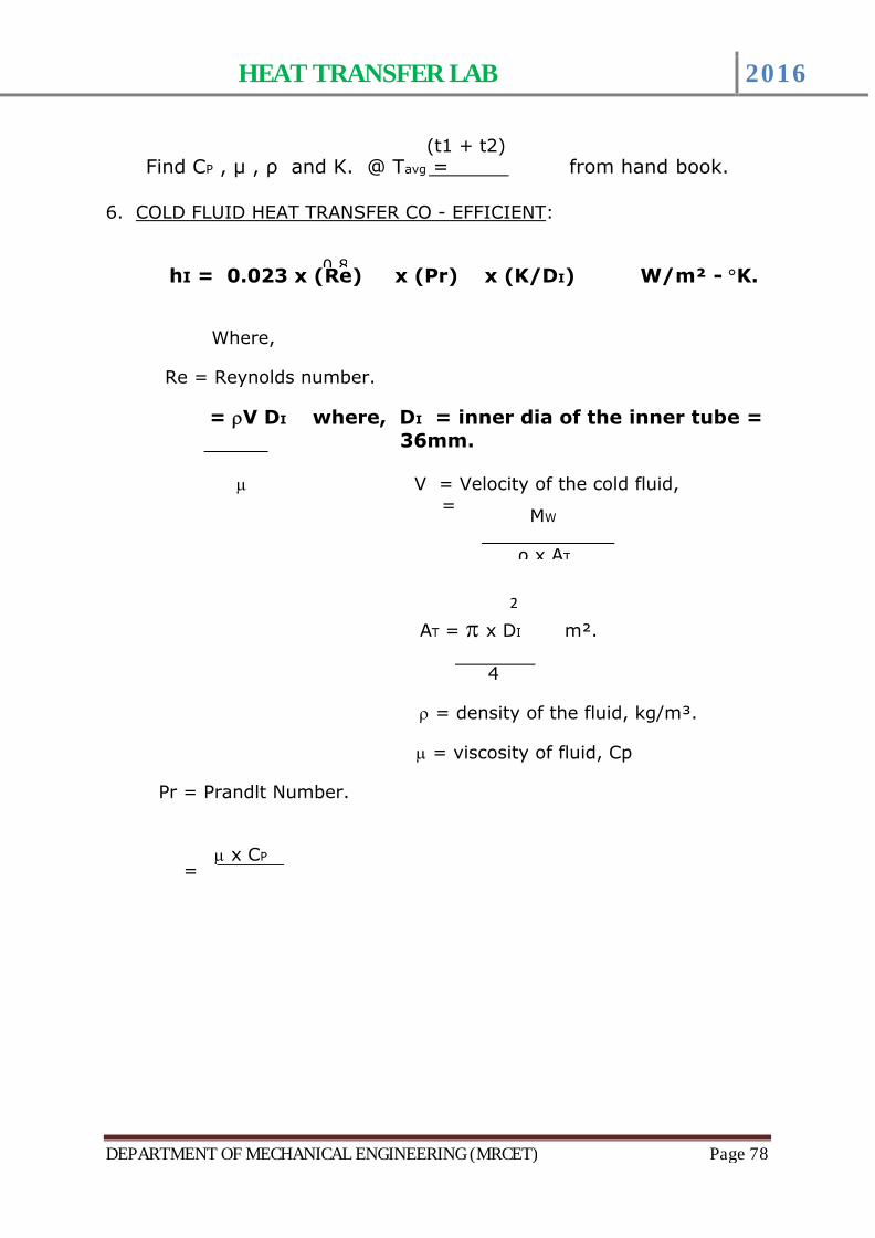
HEAT TRANSFER LAB 2016
DEPARTMENT OF MECHANICAL ENGINEERING (MRCET) Page 78
0.8
(t1 + t2)
MW
ρ x AT
2
m x CP
Find CP , μ , ρ and K. @ Tavg = from hand book.
6. COLD FLUID HEAT TRANSFER CO - EFFICIENT:
hI = 0.023 x (Re) x (Pr) x (K/DI) W/m² - ∞K.
Where,
Re = Reynolds number.
= rV DI where, DI = inner dia of the inner tube = 36mm.
m V = Velocity of the cold fluid,=
AT = p x DI m².
4
r = density of the fluid, kg/m³.
m = viscosity of fluid, Cp
Pr = Prandlt Number.
=
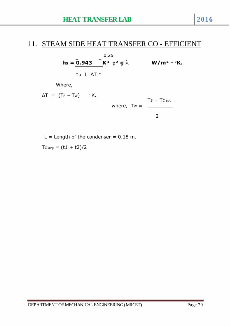
HEAT TRANSFER LAB 2016
DEPARTMENT OF MECHANICAL ENGINEERING (MRCET) Page 79
0.25
TS + TC avg
11. STEAM SIDE HEAT TRANSFER CO - EFFICIENT
hS = 0.943 K³ r² g l W/m² - ∞K.
m L ΔT
Where,
ΔT = (TS – TW) ∞K.
where, TW =
2
L = Length of the condenser = 0.18 m.
TC avg = (t1 + t2)/2
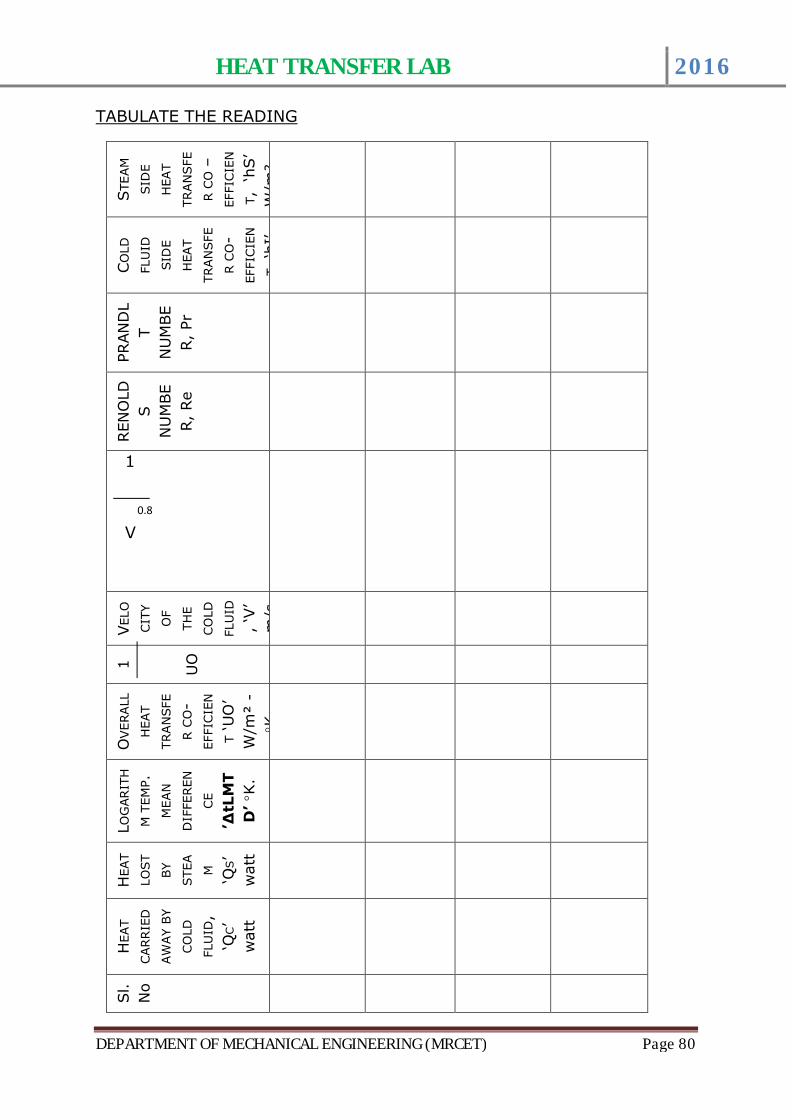
HEAT TRANSFER LAB 2016
DEPARTMENT OF MECHANICAL ENGINEERING (MRCET) Page 80
0.8
TABULATE THE READINGS
TEAM
SID
E
HEAT
TRAN
SFE
R C
O –
EFF
ICIE
N
T,
‘hS’
W/m
²
CO
LD
FLU
ID
SID
E
HEAT
TRAN
SFE
R C
O-
EFF
ICIE
N
T,
‘hI’
PRAN
DL
T
NU
MBE
R,
Pr
REN
OLD
S
NU
MBE
R,
Re
1
V
VELO
CIT
Y
OF
TH
E
CO
LD
FLU
ID
, ‘V
’ m
/s
1
UO
OVERALL
HEAT
TRAN
SFE
R C
O-
EFF
ICIE
N
T‘U
O’
W/m
² -
∞K.
LOG
ARIT
H
M T
EM
P.M
EAN
DIF
FEREN
CE
’ΔtL
MT
D’∞K
.
HEAT
LOST
BY
STEA
M ‘QS’
watt
HEAT
CARRIE
D
AW
AY
BY
CO
LD
FLU
ID,
‘QC’
watt
Sl.
No
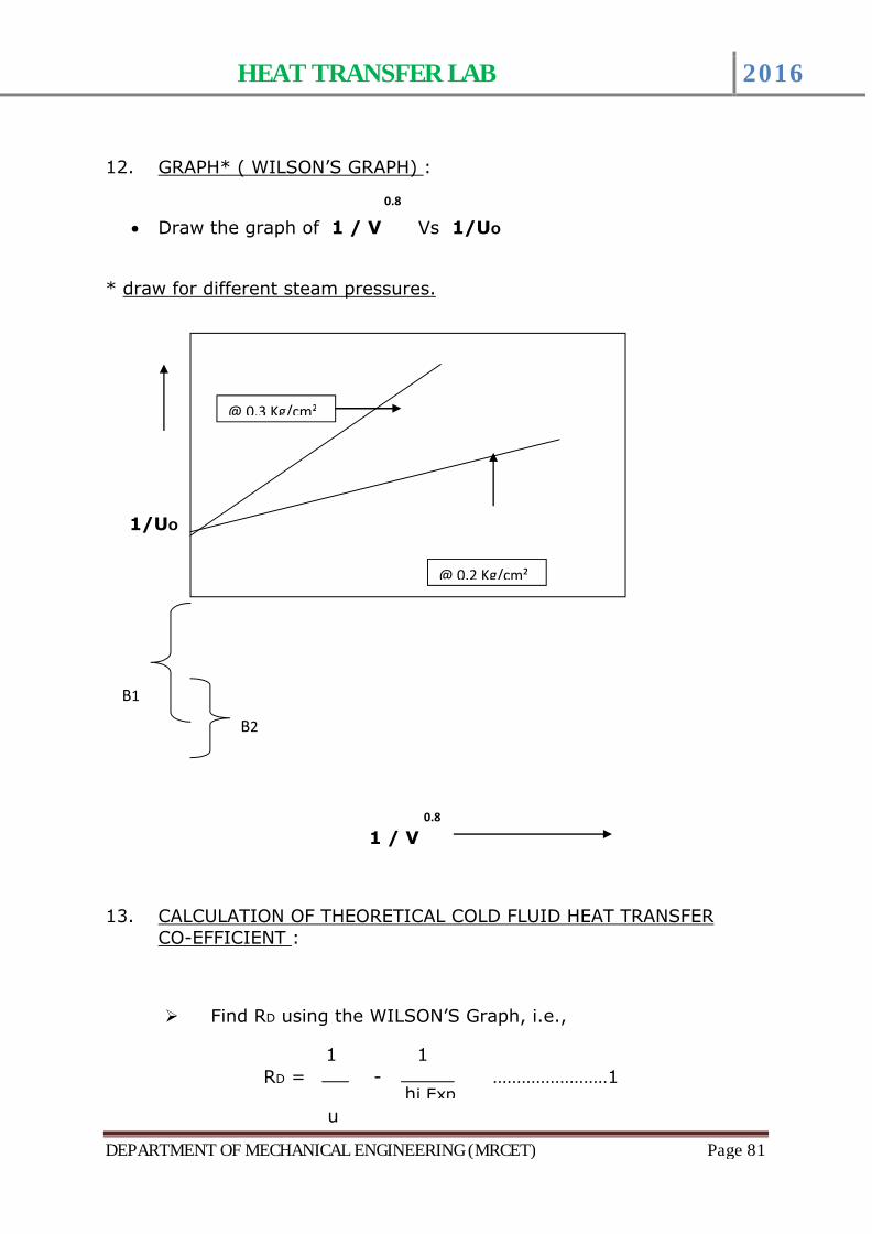
HEAT TRANSFER LAB 2016
DEPARTMENT OF MECHANICAL ENGINEERING (MRCET) Page 81
0.8
B1
1 1
hi Exp
0.8
12. GRAPH* ( WILSON’S GRAPH) :
∑ Draw the graph of 1 / V Vs 1/UO
* draw for different steam pressures.
1/UO
1 / V
13. CALCULATION OF THEORETICAL COLD FLUID HEAT TRANSFER CO-EFFICIENT :
ÿ Find RD using the WILSON’S Graph, i.e.,
RD = - ……………………1
u
@ 0.3 Kg/cm²
@ 0.2 Kg/cm²
B2
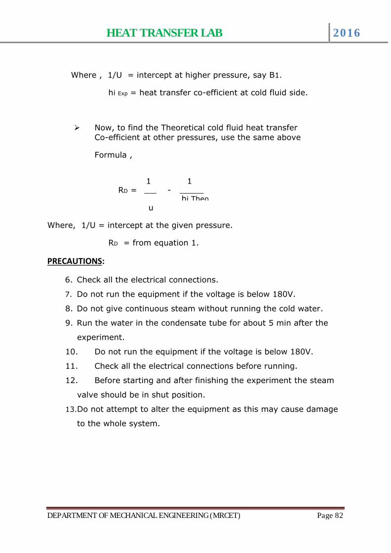
HEAT TRANSFER LAB 2016
DEPARTMENT OF MECHANICAL ENGINEERING (MRCET) Page 82
1 1
hi Theo
Where , 1/U = intercept at higher pressure, say B1.
hi Exp = heat transfer co-efficient at cold fluid side.
ÿ Now, to find the Theoretical cold fluid heat transfer Co-efficient at other pressures, use the same above
Formula ,
RD = -
u
Where, 1/U = intercept at the given pressure.
RD = from equation 1.
PRECAUTIONS:
6. Check all the electrical connections.
7. Do not run the equipment if the voltage is below 180V.
8. Do not give continuous steam without running the cold water.
9. Run the water in the condensate tube for about 5 min after the
experiment.
10. Do not run the equipment if the voltage is below 180V.
11. Check all the electrical connections before running.
12. Before starting and after finishing the experiment the steam
valve should be in shut position.
13.Do not attempt to alter the equipment as this may cause damage
to the whole system.
HEAT TRANSFER LAB 2016
DEPARTMENT OF MECHANICAL ENGINEERING (MRCET) Page 83
Reference:
3. PROCESS HEAT TRANSFER, byWareh L. McCabe
Julian C. Smith
Peter Harioth
Publication: McGraw Hill (6th edition)
4. Heat and Mass transfer by Arora & Domkundwar
5. Chemical Engineers’ Handbook, byRobert H. Perry / Cecil H. Chilton
Publication: McGraw – Hill Book Company (6th edition)