heat and water transport in soils and across the soil ......1 heat and water transport in soils and...
TRANSCRIPT

General rights Copyright and moral rights for the publications made accessible in the public portal are retained by the authors and/or other copyright owners and it is a condition of accessing publications that users recognise and abide by the legal requirements associated with these rights.
Users may download and print one copy of any publication from the public portal for the purpose of private study or research.
You may not further distribute the material or use it for any profit-making activity or commercial gain
You may freely distribute the URL identifying the publication in the public portal If you believe that this document breaches copyright please contact us providing details, and we will remove access to the work immediately and investigate your claim.
Downloaded from orbit.dtu.dk on: Jun 07, 2020
Heat and water transport in soils and across the soil-atmosphere interface: 1. Theoryand different model concepts
Vanderborght, Jan; Fetzer, Thomas; Mosthaf, Klaus; Smits, Kathleen M.; Helmig, Rainer
Published in:Water Resources Research
Link to article, DOI:10.1002/2016WR019982
Publication date:2017
Document VersionPeer reviewed version
Link back to DTU Orbit
Citation (APA):Vanderborght, J., Fetzer, T., Mosthaf, K., Smits, K. M., & Helmig, R. (2017). Heat and water transport in soilsand across the soil-atmosphere interface: 1. Theory and different model concepts. Water Resources Research,53(2), 1057-1079. https://doi.org/10.1002/2016WR019982
Heat and water transport in soils and across the soil-1
atmosphere interface – Part 1: Theory and different model 2
concepts. 3
4
Jan Vanderborght1,2*, Thomas Fetzer3, Klaus Mosthaf4, Kathleen Smits5, Rainer Helmig3. 5
6
1 Agrosphere Institute, IBG-3, Forschungszentrum Jülich GmbH, D-52425 Jülich, Germany. 7
9
2 Centre for High-Performance Scientific Computing in Terrestrial Systems, HPSC TerrSys, 10
Geoverbund ABCJ, Forschungszentrum Jülich GmbH, D-52425 Jülich. 11
12
3 Institute for Modelling Hydraulic and Environmental Systems, University of Stuttgart, 13
Pfaffenwaldring 61, 70569 Stuttgart, Germany. [email protected], 14
16
4 DTU ENVIRONMENT, Department of Environmental Engineering, Technical University of 17
Denmark, Bygningstorvet, Building 115, 2800 Kgs. Lyngby, Denmark. [email protected] 18
19
5 Center for Experimental Study of Subsurface Environmental processes, Department of Civil & 20
Environmental Engineering, Colorado Schools of Mines, 1500 Illinois Street, Golden, CO 80401, 21
USA. [email protected] 22
23
* corresponding author 24

25
Abstract 26
We review theory and model concepts for evaporation from porous media. 27
We discuss the underlying assumptions and simplifications of different approaches. 28
Approaches differ in the description of lateral transport, transport in the air phase of the 29
porous medium, and coupling at the porous medium free flow interface. 30
31
Abstract 32
Evaporation is an important component of the soil water balance. It is comprised of water flow 33
and transport processes in a porous medium that are coupled with heat fluxes and free air flow. 34
This work provides a comprehensive review of model concepts used in different research fields to 35
describe evaporation. Concepts range from non-isothermal two-phase flow, two-component 36
transport in the porous medium that is coupled with one-phase flow, two-component transport in 37
the free air flow to isothermal liquid water flow in the porous medium with upper boundary 38
conditions defined by a potential evaporation flux when available energy and transfer to the free 39
airflow are limiting or by a critical threshold water pressure when soil water availability is limiting. 40
The latter approach corresponds with the classical Richards equation with mixed boundary 41
conditions. We compare the different approaches on a theoretical level by identifying the 42
underlying simplifications that are made for the different compartments of the system: porous 43
medium, free flow and their interface, and by discussing how processes not explicitly considered 44
are parameterized. Simplifications can be grouped into three sets depending on whether lateral 45
variations in vertical fluxes are considered, whether flow and transport in the air phase in the 46
porous medium are considered, and depending on how the interaction at the interface between the 47
free flow and the porous medium is represented. The consequences of the simplifications are 48
illustrated by numerical simulations in an accompanying paper. 49
50
51
Introduction 52
The primary exchanges of heat and water that motivate global and local meteorological conditions 53
occur at the Earth’s surface. Many weather and climate phenomena (e.g., monsoons and droughts 54
) are primarily influenced by processes associated with land-atmosphere interactions in which soil 55
moisture and its control on evapotranspiration plays an important role [Seneviratne et al., 2006]. 56
More than half of the Earth’s surface is arid or semiarid having little to no vegetative cover [Katata 57
et al., 2007; Verstraete and Schwartz, 1991; Warren, 1996]. In addition, over 40% of the Earth’s 58
terrestrial surface is devoted to agricultural purposes, much of which, due to tillage practices, is 59
bare over a substantial period of the year. Properly describing the water cycle on the basis of heat 60
and water exchanges between the atmosphere and the soil surface is paramount to improving the 61
understanding of water balance conditions in these regions. Despite the importance of these 62
predictions, standard models vary in their ability to predict water fluxes, flow pathways and water 63
distribution. For instance, the fraction of globally averaged evaporation from the soil surface to 64
the total evapotranspiration from the land surface (i.e. including transpiration by the vegetation) 65
varies for different land surface models between 36% and 75% [Wang and Dickinson, 2012] with 66
a mean of 58%. 67
Understanding and controlling evaporation rates from soil is also important at much smaller scales 68
for the water management of cropped soils. For instance, in rain fed agriculture in semiarid regions, 69
where fields are cropped only once every two years and water is harvested during the non-cropped 70
year, evaporation losses during the non-cropped year determine the process or practice efficiency. 71
Evaporation may be reduced in several ways. First, by tillage, capillaries or fine pores that connect 72
the evaporating soil surface with the water stored deeper in the soil are disrupted, potentially 73
decreasing evaporation fluxes. Nevertheless, tillage may bring deeper wet soil to the soil surface 74
therefore increasing the evaporation losses. In addition, vapor diffusion may be facilitated through 75
the large interaggregate pores in tilled soils. The rougher surface of a tilled soil may also affect 76
reflectivity (albedo) and net radiation [Potter et al., 1987] and the vapor transfer between the soil 77
surface and the atmosphere. Tillage-affected soil structure alter the evaporation behavior 78
depending on the weather conditions and may either lead to larger or smaller evaporation losses 79
[Moret et al., 2007; Sillon et al., 2003; Unger and Cassel, 1991]. Another way to reduce 80
evaporation from soil is through a drying concept known as “self-mulching”, referring to the 81
development of a dry layer within the soil, which transfers moisture only in the vapor phase [Li et 82
al., 2016; Novak, 2010]. This naturally formed layer represents an effective way to maintain soil 83
moisture in the subsurface and it can be improved artificially by applying non-natural mulching 84
materials, such as gravel or plastic, to the soil surface in arid/semi-arid regions or in various 85
horticultural systems [Chung and Horton, 1987; Modaihsh et al., 1985; Tarara and Ham, 1999; 86
Yamanaka et al., 2004]. The physical mechanism is a hygroscopic equilibrium between the soil 87
vapor pressure and the atmospheric humidity, minimizing the evaporation from the mulch [Fuchs 88
and Hadas, 2011]. Several experimental studies have been conducted to investigate the effects of 89
mulch properties on soil surface evaporation processes [Diaz et al., 2005; Xie et al., 2006; Yuan et 90
al., 2009]. A negative correlation between evaporation reduction ability and grain size as well as 91
a positive correlation with mulch thickness has been recognized through sensitivity analyses of 92
experimental results. Or et al. [2013] reviewed the physical processes that control evaporation 93
processes from porous media and focused on the role of capillary and viscous forces and of 94
diffusive transfers in the porous medium and across the interface between the porous medium and 95
the free flow. This approach allowed them to relate evaporation process to microscopic properties 96
of the porous medium. In simulation models that operate at the continuum scale, these small scale 97
processes and properties must be included in macroscopic properties and constitutive relations 98
between properties, states and fluxes. 99
Practical and theoretical limitations of modeling efforts at the continuum scale are often magnified 100
at the land-atmosphere interface, where water and energy fluxes are highly dynamic and 101
dramatically influenced by changes in temperature and moisture gradients and direction of flows 102
[Lehmann et al., 2012]. The flow and transport behavior at the soil surface is affected by the 103
conditions in the atmosphere (e.g., humidity, temperature, wind velocity, solar radiation) and by 104
the soil thermal and hydraulic properties and states (e.g., thermal and hydraulic conductivity, 105
porosity, capillary pressure, temperature, vapor pressure), all of which are strongly coupled [Sakai 106
et al., 2011]. For most subsurface models, the soil surface serves as the upper boundary to the 107
porous medium domain and is characterized using prescribed flux terms that serve as sources and 108
sinks. Similarly, in most atmospheric models, the vadose zone serves as a lower boundary with 109
prescribed fluxes. Such an approach is a simplification of the interaction processes at the common 110
interface of the two flow compartments. Although widely used due to its simplicity and ease of 111
use, such an approach has been shown by both atmospheric and hydrogeological scientists to 112
misrepresent flux conditions, resulting in model prediction errors [Seager et al., 2007]. 113
In practice, the Richards equation is the most frequently used conceptual model to describe water 114
movement within the vadose zone, and to simulate water and energy exchanges between the land 115
surface and the atmosphere at the global scale. However, it is mostly used in a form that considers 116
only isothermal liquid water flow but neglects vapor diffusion and air flow in the porous medium 117
and the effects of temperature gradients on flow and transport processes. Although the application 118
of Richards equation has been successful to describe soil water fluxes at various scales (e.g. 119
[Mortensen et al., 2006; Nieber and Walter, 1981; Schoups et al., 2005; Vereecken et al., 1991]), 120
there may arise conditions in which the non-considered processes become relevant. The predictive 121
capacities of the Richards equation to evaluate, for instance, surface manipulations that influence 122
air flow, vapor transport and thermal regimes in the porous medium could therefore be questioned. 123
Also for global scale simulations, the consideration of additional processes such as vapor transport 124
in the soil and transport driven by thermal gradients are receiving more attention to reduce the bias 125
in bare soil evaporation predictions that are observed in these models [Tang and Riley, 2013b]. 126
Most Richards equation based models assume that soil water flux is one-dimensional (i.e. water 127
flow only occurs vertically), thus neglecting any lateral variations in fluxes within the soil profiles 128

and also at the soil-atmosphere interface. Three-dimensional solutions of the Richards equation 129
have been used to investigate the effect of soil heterogeneity and hence dimensionality on flow 130
and transport processes. However, these simulation studies focused mostly on conditions when 131
flow was directed downward (infiltration). For certain problems of practical relevance, e.g. 132
evaporation from surfaces that are partially covered by mulches or row crops, a multidimensional 133
description of upward flow in the soil is used [Bristow and Horton, 1996; Horton, 1989]. The few 134
studies that also looked at heterogeneous flow and transport for upward directed flow 135
(evaporation) reported conceptual problems with the definition of the boundary conditions at the 136
soil surface [Bechtold et al., 2012; Schlüter et al., 2012]. 137
Boundary conditions for the Richards equation are determined as a uniform flux boundary 138
condition, which is derived by solving a surface energy balance, as long as a threshold pressure 139
head is not reached. When the soil dries out and the critical pressure head is reached, the boundary 140
condition is switched to a pressure head boundary condition. First, the definition of this critical 141
pressure head is often debated. Second, for a heterogeneous soil surface in which patches of wet 142
soil alternate with dried out areas, the evaporation rate from the wet patches may increase 143
compared to the evaporation from a uniformly wet surface due to lateral exchange processes in the 144
air flow (free flow) or in the porous medium. The effect of lateral exchange processes in the free 145
flow on evaporation leads to the so-called ‘oasis effect’ and has been quantified to evaluate, for 146
instance, the effect of the size of pores [Assouline et al., 2010; Shahraeeni and Or, 2012], 147
evaporation pans [Brutsaert and Yu, 1968], or ponds and lakes [Harbeck, 1962]. Lateral water and 148
heat fluxes in heterogeneous porous media may lead to a larger water loss due to evaporation from 149
a porous medium compared to the water loss from a homogeneous medium [Lehmann and Or, 150
2009; Shahraeeni and Or, 2011]. 151
152
The general objective of this paper is to theoretically compare various model concepts used to 153
describe evaporation processes from soils at the continuum scale. Modeling concepts vary in 154

complexity from fully coupled free flow and porous media flow representations to reduced 155
complexity models such as those using Richards equations. First, we present the modeling 156
concepts for flow and transport in the porous medium (i.e. soil), the free flow (i.e. atmosphere), 157
and the coupling of the porous medium with the free flow (Figure 1). As different scientific 158
communities (soil physics, hydrology, atmospheric sciences and micrometeorology, and fluid 159
mechanics in porous media and in free flow) place different emphasis on the porous medium versus 160
the free flow, oftentimes the coupling is strongly simplified or overlooked. This often leads to 161
inconsistencies in the degree of detail with which processes are described in the porous medium 162
or in the free flow (e.g. 3-D flow in the porous medium coupled with a 1-D transfer resistance to 163
describe the exchange with the free flow) and misunderstandings between communities about the 164
importance of different processes. Therefore, the first objective of this work is to present a 165
comprehensive set of equations that describe all processes in both compartments (free flow and 166
porous medium) and all relevant coupling conditions. This is followed a discussion of common by 167
simplifications that lead to models of reduced complexity. Table 1, provides an overview of the 168
constitutive equations for the two compartments, their interface and potential simplifications. 169
What can be observed immediately from Table 1 is that the variables and parameters used in the 170
various approaches differ significantly. 171
The second objective is to show the similarities and differences between the different approaches 172
by deriving the variables and parameters based on a theoretical analysis of the comprehensive 173
model. Model simplifications and 'fixes' are explained in detail, thus allowing for a full 174
understanding of all approaches and for a classification of the simplifications. 175
In an accompanying paper, the consequences of these simplifications on the predictions of 176
evaporation are investigated for two sets of exemplary simulations. 177
178
Coupled heat and water flow in porous media: overview of 179
concepts and simplifications at the continuum scale 180
In this section, we introduce the model concepts used to describe heat and water fluxes in soils at 181
the continuum scale. From the general balance equations, simplified equations are derived and the 182
assumptions behind these simplifications are discussed. The employed constitutive equations are 183
presented. 184
185
Balance equations: 186
A full description of water and vapor transport in a porous medium requires a description of flow 187
of the two fluid phases, liquid and gas {𝑙, 𝑔}, and of the transport of the components, water and 188
dry air {𝑤, 𝑎} in each of the two phases. For simplicity, we consider air as a pseudo-component 189
consisting of oxygen, nitrogen and other gases except vapor, which is regarded as separate 190
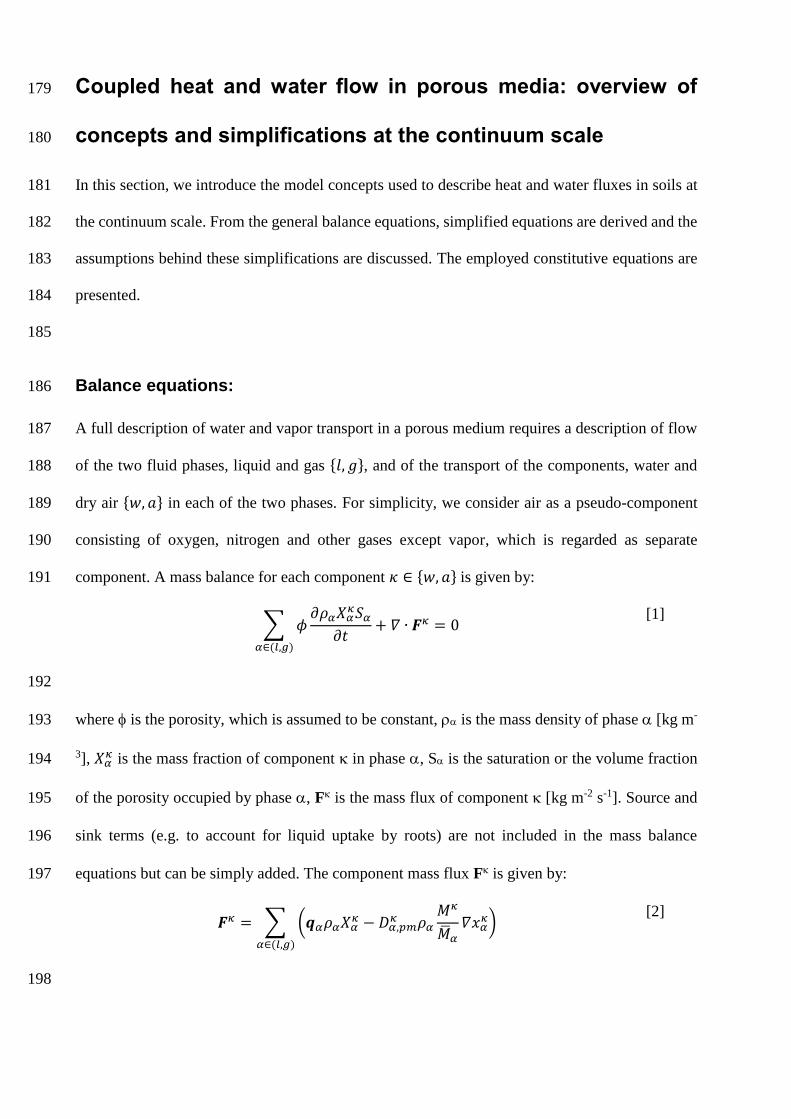
component. A mass balance for each component 𝜅 ∈ {𝑤, 𝑎} is given by: 191
∑ 𝜙𝜕𝜌𝛼𝑋𝛼
𝜅𝑆𝛼𝜕𝑡
+ 𝛻 ∙ 𝑭𝜅 = 0
𝛼∈(𝑙,𝑔)
[1]
192
where is the porosity, which is assumed to be constant, is the mass density of phase [kg m-193
3], 𝑋𝛼𝜅 is the mass fraction of component in phase , S is the saturation or the volume fraction 194
of the porosity occupied by phase , F is the mass flux of component [kg m-2 s-1]. Source and 195
sink terms (e.g. to account for liquid uptake by roots) are not included in the mass balance 196
equations but can be simply added. The component mass flux F is given by: 197
𝑭𝜅 = ∑ (𝒒𝛼𝜌𝛼𝑋𝛼𝜅 − 𝐷𝛼,𝑝𝑚
𝜅 𝜌𝛼𝑀𝜅
�̅�𝛼𝛻𝑥𝛼
𝜅)
𝛼∈(𝑙,𝑔)
[2]
198
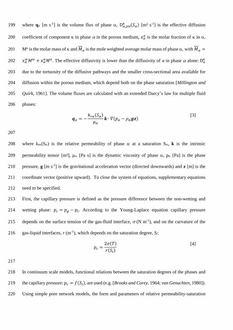
where q [m s-1] is the volume flux of phase D𝛼,pm𝜅 (𝑆𝛼) [m² s-1] is the effective diffusion 199
coefficient of component in phase in the porous medium, 𝑥𝛼𝜅 is the molar fraction of in , 200
M is the molar mass of and 𝑀𝛼 is the mole weighted average molar mass of phase with𝑀𝛼 =201
𝑥𝛼𝑤𝑀𝑤 + 𝑥𝛼
𝑎𝑀𝑎. The effective diffusivity is lower than the diffusivity of in phase alone: D𝛼𝜅 202
due to the tortuosity of the diffusive pathways and the smaller cross-sectional area available for 203
diffusion within the porous medium, which depend both on the phase saturation [Millington and 204
Quirk, 1961]. The volume fluxes are calculated with an extended Darcy’s law for multiple fluid 205
phases: 206
𝒒𝛼 = −𝑘𝑟𝛼(𝑆𝛼)
𝜇𝛼𝒌 ∙ 𝛻(𝑝𝛼 − 𝜌𝛼𝒈𝒛)
[3]
207
where kr(S) is the relative permeability of phase at a saturation S, k is the intrinsic 208
permeability tensor [m²], [Pa s] is the dynamic viscosity of phase , p [Pa] is the phase 209
pressure, g [m s-2] is the gravitational acceleration vector (directed downwards) and z [m] is the 210
coordinate vector (positive upward). To close the system of equations, supplementary equations 211
need to be specified. 212
First, the capillary pressure is defined as the pressure difference between the non-wetting and 213
wetting phase: 𝑝𝑐 = 𝑝𝑔 − 𝑝𝑙. According to the Young-Laplace equation capillary pressure 214
depends on the surface tension of the gas-fluid interface, (N m-1), and on the curvature of the 215
gas-liquid interfaces, r (m-1), which depends on the saturation degree, Sl: 216
𝑝𝑐 =2𝜎(𝑇)
𝑟(𝑆𝑙)
[4]
217
In continuum scale models, functional relations between the saturation degrees of the phases and 218
the capillary pressure: 𝑝𝑐 = 𝑓(𝑆𝑙), are used (e.g. [Brooks and Corey, 1964; van Genuchten, 1980]). 219
Using simple pore network models, the form and parameters of relative permeability-saturation 220

functions were linked to the capillary pressure-saturation functions. In the Mualem van-Genuchten 221
model, cylindrical pores are assumed. Assuming other pore geometries, e.g. triangular pores, lead 222
to considerably higher permeabilities under dry soil conditions [Diamantopoulos and Durner, 223
2015; Peters and Durner, 2008; Tuller and Or, 2001]. Also, retention functions which describe 224
the dry range of the water retention curve better than the van Genuchten function have been 225
proposed and tested (e.g. [Lu et al., 2008]) and might be more suited to describe evaporation 226
processes. 227
Second, the sum of all phase saturations and of all mass fractions equals 1. 228
Third, a chemical equilibrium of a component between different phases may be assumed. This sets 229
a relation between the mole fraction of air in the liquid phase, 𝑥𝑙𝑎 , and the partial air pressure 𝑝𝑔
𝑎 230
[Pa] in the gas phase using Henry’s law. Furthermore, a relation between the vapor pressure and 231
the capillary pressure is given by Kelvin’s equation [Edlefsen and Anderson, 1943]: 232
𝑝𝑔𝑤 = 𝑝𝑔,sat
𝑤 𝑒𝑥𝑝 (−𝑝𝑐𝑀
𝑤
𝜌𝑙𝑅𝑇)
[5]
233
where 𝑝𝑔,sat𝑤 [Pa] is the temperature-dependent saturated vapor pressure, Mw is the molecular 234
weight of water [kg mol-1], R is the universal gas constant [J mol-1 K-1] and T [K] is the absolute 235
temperature. The relation between the capillary pressure and the water vapor pressure only holds 236
for dilute solutions. When the concentration of salts increases, also the osmotic soil water potential 237
must be considered in Eq. [5] and an additional component equation for salt transport in the liquid 238
phase and chemical equilibrium equations describing salt precipitation and dissolution must be 239
included. We will not consider osmotic effects in the following but refer to [Nassar and Horton, 240
1997; 1999] who describe a model that considers coupled heat, vapor, liquid water, and solute 241
transport. The mole fractions and partial pressures can be directly related to the mass fractions 242
𝑋𝛼𝜅 using molar weights and the ideal gas law: 243
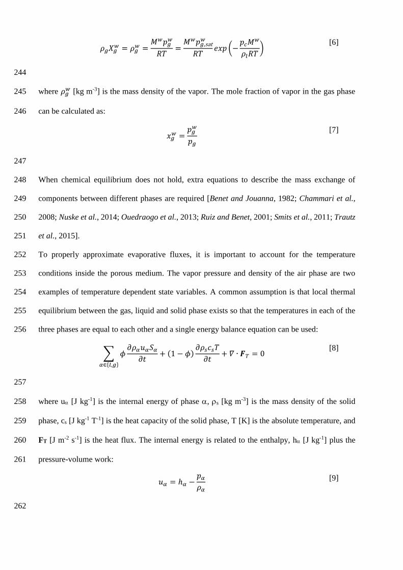
𝜌𝑔𝑋𝑔𝑤 = 𝜌𝑔
𝑤 =𝑀𝑤𝑝𝑔
𝑤
𝑅𝑇=𝑀𝑤𝑝𝑔,sat
𝑤
𝑅𝑇𝑒𝑥𝑝 (−
𝑝𝑐𝑀𝑤
𝜌𝑙𝑅𝑇)
[6]
244
where 𝜌𝑔𝑤 [kg m-3] is the mass density of the vapor. The mole fraction of vapor in the gas phase 245
can be calculated as: 246
𝑥𝑔𝑤 =
𝑝𝑔𝑤
𝑝𝑔
[7]
247
When chemical equilibrium does not hold, extra equations to describe the mass exchange of 248
components between different phases are required [Benet and Jouanna, 1982; Chammari et al., 249
2008; Nuske et al., 2014; Ouedraogo et al., 2013; Ruiz and Benet, 2001; Smits et al., 2011; Trautz 250
et al., 2015]. 251
To properly approximate evaporative fluxes, it is important to account for the temperature 252
conditions inside the porous medium. The vapor pressure and density of the air phase are two 253
examples of temperature dependent state variables. A common assumption is that local thermal 254
equilibrium between the gas, liquid and solid phase exists so that the temperatures in each of the 255
three phases are equal to each other and a single energy balance equation can be used: 256
∑ 𝜙𝜕𝜌𝛼𝑢𝛼𝑆𝛼𝜕𝑡
+ (1 − 𝜙)𝜕𝜌𝑠𝑐𝑠𝑇
𝜕𝑡+ 𝛻 ∙ 𝑭𝑇 = 0
𝛼∈{𝑙,𝑔}
[8]
257
where u [J kg-1] is the internal energy of phase , s [kg m-3] is the mass density of the solid 258
phase, cs [J kg-1 T-1] is the heat capacity of the solid phase, T [K] is the absolute temperature, and 259
FT [J m-2 s-1] is the heat flux. The internal energy is related to the enthalpy, h [J kg-1] plus the 260
pressure-volume work: 261
𝑢𝛼 = ℎ𝛼 −𝑝𝛼𝜌𝛼
[9]
262
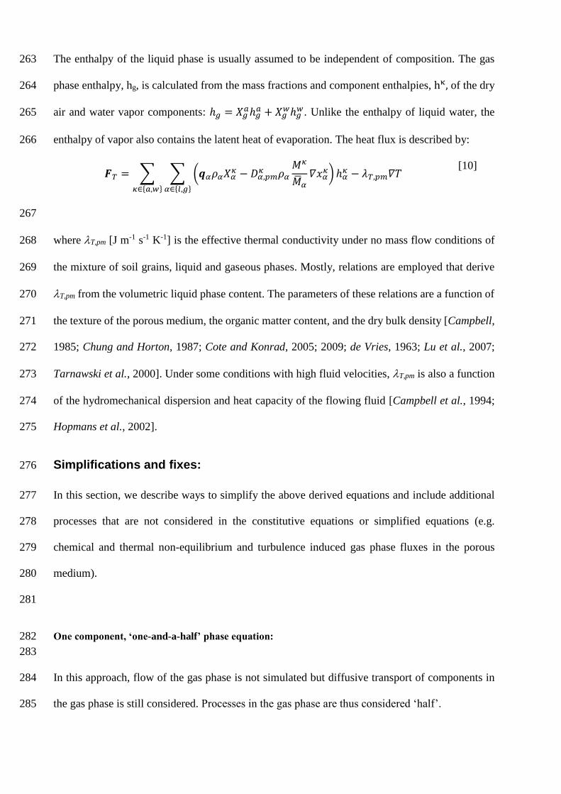
The enthalpy of the liquid phase is usually assumed to be independent of composition. The gas 263
phase enthalpy, hg, is calculated from the mass fractions and component enthalpies, hκ, of the dry 264
air and water vapor components: ℎ𝑔 = 𝑋𝑔𝑎ℎ𝑔
𝑎 + 𝑋𝑔𝑤ℎ𝑔
𝑤. Unlike the enthalpy of liquid water, the 265
enthalpy of vapor also contains the latent heat of evaporation. The heat flux is described by: 266
𝑭𝑇 = ∑ ∑ (𝒒𝛼𝜌𝛼𝑋𝛼𝜅 − 𝐷𝛼,𝑝𝑚
𝜅 𝜌𝛼𝑀𝜅
�̅�𝛼𝛻𝑥𝛼
𝜅) ℎ𝛼𝜅 − 𝜆𝑇,𝑝𝑚𝛻𝑇
𝛼∈{𝑙,𝑔}𝜅∈{𝑎,𝑤}
[10]
267
where T,pm [J m-1 s-1 K-1] is the effective thermal conductivity under no mass flow conditions of 268
the mixture of soil grains, liquid and gaseous phases. Mostly, relations are employed that derive 269
T,pm from the volumetric liquid phase content. The parameters of these relations are a function of 270
the texture of the porous medium, the organic matter content, and the dry bulk density [Campbell, 271
1985; Chung and Horton, 1987; Cote and Konrad, 2005; 2009; de Vries, 1963; Lu et al., 2007; 272
Tarnawski et al., 2000]. Under some conditions with high fluid velocities, T,pm is also a function 273
of the hydromechanical dispersion and heat capacity of the flowing fluid [Campbell et al., 1994; 274
Hopmans et al., 2002]. 275
Simplifications and fixes: 276
In this section, we describe ways to simplify the above derived equations and include additional 277
processes that are not considered in the constitutive equations or simplified equations (e.g. 278
chemical and thermal non-equilibrium and turbulence induced gas phase fluxes in the porous 279
medium). 280
281
One component, ‘one-and-a-half’ phase equation: 282
283
In this approach, flow of the gas phase is not simulated but diffusive transport of components in 284
the gas phase is still considered. Processes in the gas phase are thus considered ‘half’. 285

This approach assumes that the pressure in the gas phase, pg, is uniform and constant with time 286
which results in the independence of the liquid phase pressure from flow in the gas phase. This 287
assumption is justified based on the magnitude of the gas phase viscosity compared to that of the 288
liquid phase (smaller by a factor 50). Therefore, Eq. [3] is only solved for the liquid phase and gas 289
fluxes can be calculated directly from the change in the liquid phase saturation over time. 290
Secondly, only the flux of the water component is considered, assuming that the water component 291
flux is not influenced by the dry air concentrations in the two phases. For the liquid phase, this 292
approximation hinges on the fact that the mass fraction of water in the liquid phase is close to one: 293
𝑋𝑙𝑤 ≈ 1. For the gas phase, the vapor pressure that is in equilibrium with the liquid phase is 294
calculated from the capillary pressure (Eq. [5]), which depends only on the liquid phase pressure 295
since the gas phase pressure is assumed to be constant. The vapor concentration is calculated using 296
the ideal gas law (because 𝑋𝑙𝑤 ≈ 1 ) (Eq. [6]) and thus independent of the dry air concentration in 297
the gas phase. Thirdly, it is assumed that advective fluxes of components in the gas phase can be 298
neglected, 𝒒𝒈𝜌𝑔𝑋𝑔𝑤 ≈ 0, compared with the diffusive fluxes. Finally, this approach assumes that 299
gradients in the molar volume of the gas phase can be neglected and that the mass density of the 300
liquid phase is constant. As a result of these assumptions, the water component flux equation (Eq. 301
[2]) reduces to: 302
𝑭𝑤 ≈ 𝒒𝑙𝜌𝑙 −𝑫𝑔,pm𝑤 (𝑆𝑔)𝛻𝜌𝑔
𝑤 [11]
303
The mass balance equation for water simplifies to: 304
𝜙𝜕𝜌𝑔𝑋𝑔
𝑤𝑆𝑔
𝜕𝑡+ 𝜙
𝜕𝜌𝑙𝑆𝑙𝜕𝑡
− 𝛻 ∙ [𝜌𝑙𝑘𝑟𝑙(𝑆𝑙)
𝜇𝑙𝒌𝛻(𝑝𝑙 − 𝜌𝑙𝒈𝒛)] − 𝛻 ∙ [𝑫𝑔,pm
𝑤 𝛻𝜌𝑔𝑤] = 0
[12]
305
This is the basic equation used by the soil physics community to describe non-isothermal liquid 306
water flow and water vapor transport in soils. However, it is usually expressed in the following 307
form [Milly, 1982; Saito et al., 2006]: 308

𝜕𝜃𝑙𝜕𝑡+𝜕𝜃𝑣𝜕𝑡
= 𝛻 ∙ [(𝑲𝑙,𝜓 +𝑲𝑣,𝜓)𝜎(𝑇)
𝜎(𝑇𝑟𝑒𝑓)𝛻𝜓|𝑇𝑟𝑒𝑓 +𝑲𝑙,𝜓𝒆𝒛] +
𝛻 ∙ (𝑲𝑙,𝑇 +𝑲𝑣,𝑇)𝛻𝑇
[13]
309
where l = Sl is volumetric liquid water content and v the water vapor content expressed in 310
volume of liquid water (𝜃𝑣 = 𝜙𝜌𝑔𝑤𝑆𝑔/𝜌𝑙), Kl,x and Kv,x are the hydraulic conductivities for liquid 311
water flow and vapor transport, respectively, Kx, [m s-1] and Kx,T [m² K-1 s-1] are the isothermal 312
and thermal hydraulic conductivities, respectively, ez is the unit coordinate vector in the vertical 313
direction, and |Tref (m) is the pressure head of the liquid phase at the reference temperature Tref. 314
The first term on the right hand side of Eq. [13] represents the total water flow due to pressure 315
head gradients under isothermal conditions and due to gravity. Since the pressure head gradients 316
are defined at a reference temperature, a standard relation between l and |Tref can be used. The 317
second term on the right hand side accounts for the total water fluxes that are generated by a 318
thermal gradient. 319
In the following section, the relationships between the hydraulic properties Kxy, the variables v, 320
l, |Tref, and T, the fluid properties, and the effective diffusion coefficients and permeability are 321
presented and the equality between Eqs. [12] and [13] elucidated. 322
The pressure head of the water phase can be defined in terms of the capillary pressure pc as: 323
𝑝𝑐 = −𝜓𝑔𝜌𝑙 [14]
324
Assuming a uniform and constant gas phase pressure and liquid phase density, the water pressure 325
gradient can be replaced by the pressure head gradient multiplied by a constant factor gl. 326
Considering Eq. [4] the spatial gradient of can be written as: 327
𝛻𝜓(𝜃𝑙 , 𝑇) =𝜕𝜓
𝜕𝜃𝑙|𝑇
𝛻𝜃𝑙 +𝜕𝜓
𝜕𝜎|𝜃𝑙
𝜕𝜎
𝜕𝑇𝛻𝑇
[15]
or 328

𝛻𝜓(𝜃𝑙 , 𝑇) =𝜕𝜓
𝜕𝜃𝑙|𝑇
𝛻𝜃𝑙 +𝜓
𝜎|𝜃𝑙
𝜕𝜎
𝜕𝑇𝛻𝑇
[16]
𝛻𝜓(𝜃𝑙 , 𝑇) =𝜕𝜓
𝜕𝜃𝑙|𝑇
𝜕𝜃𝑙𝜕𝜓|Tref
𝛻𝜓|Tref +𝜓Tref𝜎(𝑇ref)
|𝜃𝑙
𝜕𝜎
𝜕𝑇𝛻𝑇
[17]
𝛻𝜓(𝜃𝑙, 𝑇) =𝜎(𝑇)
𝜎(𝑇ref)𝛻𝜓|Tref +
𝜓Tref𝜎(𝑇ref)
|𝜃𝑙
𝜕𝜎
𝜕𝑇𝛻𝑇
[18]
329
The first term of the right hand side of Eq. [16] represents the gradient in pressure head due to a 330
gradient in the volumetric water content under isothermal conditions. Using the relationship 331
between pressure head and volumetric water content at a reference temperature, Tref, this term can 332
be rewritten in terms of a pressure head gradient at a reference temperature (first term of Eq. [18]). 333
The second term in Eq. [16] represents the gradient in pressure head due to a temperature gradient 334
at a given volumetric water content l. This term can also be rewritten in terms of a pressure head 335
for a given water content l at a reference temperature (Eq. [18]). 336
In a similar vein, the gradient 𝛻𝜌𝑔𝑤can be written as: 337
𝛻𝜌𝑔𝑤(𝜓, 𝑇) =
𝜕𝜌𝑔𝑤
𝜕𝜓|𝑇
𝜎(𝑇)
𝜎(𝑇ref)𝛻𝜓|Tref +
𝜕𝜌𝑔𝑤
𝜕𝑇|𝜓
𝛻𝑇 [19]
338
Including Equations [14], [18], and [19] in Eq. [12] leads to the following equation: 339
𝜕𝜃𝑣𝜕𝑡
+𝜕𝜃𝑙𝜕𝑡
= 𝛻 ∙ [(𝑲𝑙,𝜓 +𝑫𝑔,𝑝𝑚𝑤 (𝑆𝑔)
𝜌𝑙
𝜕𝜌𝑔𝑤
𝜕𝜓|𝑇
)𝜎(𝑇)
𝜎(𝑇ref)𝛻𝜓|Tref +𝑲𝑙,𝜓𝒆𝒛]
+ 𝛻 ∙ [(𝑲𝑙,𝜓𝜓Tref𝜎(𝑇ref)
|𝜃𝑗
𝜕𝜎
𝜕𝑇+𝑫𝑔,𝑝𝑚𝑤 (𝑆𝑔)
𝜌𝑙
𝜕𝜌𝑔𝑤
𝜕𝑇|𝜓
)𝛻𝑇]
[20]
340
Using the relation between the vapor density, capillary pressure and temperature (Eq. [6]) and 341
defining the saturated vapor density 𝜌𝑔,𝑠𝑎𝑡𝑤 [kg m-3] and the relative humidity of the air Hr = 342
𝜌𝑔𝑤 𝜌𝑔,𝑠𝑎𝑡
𝑤⁄ it follows from Eq. [20] that the conductivities in Eq. [13] are defined as: 343

𝑲𝑙,𝜓 =𝜌𝑙𝑔𝑘𝑟𝑙(𝑆𝑙)
𝜇𝑙𝒌
[21]
𝑲𝑣,𝜓 =𝑔𝑀𝑤𝜌𝑔,𝑠𝑎𝑡
𝑤 𝐻𝑟
𝜌𝑙𝑅𝑇𝑫𝑔,𝑝𝑚𝑤 (𝑆𝑔)
[22]
𝑲𝑙,𝑇 = 𝑲𝜓Tref𝜎(𝑇ref)
|𝜃𝑙
𝜕𝜎
𝜕𝑇
[23]
𝑲𝑣,𝑇 =𝐻𝑟𝜌𝑙
𝜕𝜌𝑔,𝑠𝑎𝑡𝑤
𝜕𝑇𝑫𝑔,𝑝𝑚𝑤 (𝑆𝑔)
[24]
344
Eq. [13] relies on the assumption of local thermal equilibrium. However, the temperature of the 345
air, water and soil particles may differ due to the difference in thermal properties of these phases 346
and rapid changes of soil surface temperatures. Therefore, it is argued that the temperature gradient 347
in the soil air is often larger than the gradient of the mean temperature over the different phases. 348
The effective diffusion of water vapor in soil may be larger than that of other gases since water 349
vapor may condense and evaporate from capillary held water pockets (i.e. “liquid bridges” or 350
“capillary islands”), thus blocking the diffusive transport of other gases [Philip and De Vries, 351
1957]. These effects have been used to explain observations of enhanced vapor transport compared 352
to Fick’s law of diffusion [Gurr et al., 1952; Rollins et al., 1954; Taylor and Cavazza, 1954]. To 353
account for this, Kv,T is multiplied by an enhancement factor [de Vries, 1958; Philip and De 354
Vries, 1957] described by empirical formulations (e.g. [Campbell, 1985; Cass et al., 1984]). This 355
approach has been widely used and accepted to calculate heat and water flow in soils (e.g. [Hadas, 356
1977; Reshetin and Orlov, 1998; Rose, 1967; Shepherd and Wiltshire, 1995; Sophocleous, 1979]). 357
However, the validity or need for vapor enhancement has been questioned [Ho and Webb, 1998; 358
Shokri et al., 2009; Smits et al., 2013]. 359
In addition ot vapor enhancement, an enhancement of the liquid flow that is induced by thermal 360
gradients has been proposed [Noborio et al., 1996; Saito et al., 2006]. This enhancement is 361
attributed to the change in surface tension that results from changes in soil water composition 362

(ionic strength, concentration of organic surfactants) with temperature. Thermal enhancement is 363
accounted for by multiplying Kl,T (Eq. [23]) by a non-dimensional empirical ‘gain factor’ ranging 364
in value from 0 to 10 [Nimmo and Miller, 1986]. 365
In Eqs. [18] and [19], the gradients in the pressure head and vapor mass density were written in 366
terms of gradients in temperature and pressure head at a reference temperature assuming that the 367
change in water content with pressure head, 𝜕𝜃𝑙
𝜕𝜓, is only a function of the surface tension, , and 368
temperature effects were attributed to changes in with temperature. But, the relationship between 369
l and also depends on the interaction between the solid and liquid phase (i.e. the contact angle 370
between the liquid-gas surface and the solid phase or solid phase wettability) which may also 371
change with temperature [Bachmann et al., 2002]. Therefore, it is important to note that for non-372
wettable soils temperature effects on solid-liquid phase interactions should be included in the 373
model to predict reduced evaporation from non-wettable soils or reduced water redistribution due 374
to temperature gradients in non wettable soil [Bachmann et al., 2001; Davis et al., 2014]. 375
376
Isothermal one component, ‘one-and-a-half’ phase equation: 377
When water fluxes are considered over a longer period of time (i.e. multiple days), it may be 378
argued that the temporal average of the temperature gradients cancels out due to diurnal variations 379
in temperature. This also results in the temperature gradient driven fluxes canceling out [Milly, 380
1984]. Based on this assumption, the flow equation can be simplified to an isothermal equation 381
and flow due to a temperature gradient (i.e. in Eq. [13]) can be neglected so that for a 1-D flow 382
process (as routinely assumed in soils), the following equation is obtained: 383
384
𝜕𝜃𝑣𝜕𝑡
+𝜕𝜃𝑙𝜕𝑡
=𝜕
𝜕𝑧∙ [(𝐾𝑙,𝜓 + 𝐾𝑣,𝜓)
𝜕𝜓
𝜕𝑧+ 𝐾𝑙,𝜓]
[25]
385

Isothermal one component one phase equation, Richards equation 386
Finally, when vapor transport is neglected, the classical Richards equation is obtained: 387
𝜕𝜃𝑙𝜕𝑡
=𝜕
𝜕𝑧∙ [𝐾𝑙,𝜓
𝜕𝜓
𝜕𝑧+ 𝐾𝑙,𝜓]
[26]
388
Flow and transport processes in the atmosphere 389
In this section, the free flow balance equations are described and then possible simplifications are 390
presented and discussed. 391
Balance equations 392
In the context of evaporation processes from soils, flow conditions in the free flow are mostly 393
turbulent. Turbulent flow is usually highly irregular with chaotic fluctuations of the local velocity, 394
pressure, concentration and temperature [Bird et al., 2007]. These fluctuations are caused by 395
vortices or eddies, which occur over a wide range of length scales. It is possible to simulate all of 396
these phenomena, but it requires the resolution of eddies on all scales and has therefore high 397
computational costs. To reduce these costs, turbulence can be parameterized rather than simulated 398
explicitly. The most commonly used parametrization approach is the so-called Reynolds 399
averaging. The basic assumption is that turbulent fluctuating quantities can be split in a temporal 400
average 𝑣 and a fluctuating part 𝑣′. This is called the Reynolds decomposition: 401
𝑣𝑔 = 𝑣𝑔 + 𝑣′𝑔 , 𝑝𝑔 = 𝑝𝑔 + 𝑝
′𝑔, 𝑥𝑔
𝜅 = 𝑥𝑔𝜅 + 𝑥𝑔
𝜅′, 𝑇 = 𝑇 + 𝑇′ [27]
where vg [m s-1] is the gas velocity. 402
After replacing the instantaneous values in the balance equations by the sum of the average and 403
fluctuating parts, the balance equations are averaged over time. For a more detailed overview on 404
turbulence modeling and the Reynolds averaging procedure, we refer the reader to standard fluid 405
dynamic textbooks (e.g. [Bird et al., 2007; Wilcox, 2006]). The total mass balance for the gas phase 406
is: 407

𝜕𝜌𝑔
𝜕𝑡+ 𝛻 ∙ [𝜌𝑔 𝒗𝑔] = 0
[28]
The momentum balance is: 408
𝜕(𝜌𝑔𝒗𝑔)
𝜕𝑡+ 𝛻 ∙
[
𝜌𝑔 𝒗𝑔 𝒗𝑔 + 𝜌𝑔𝒗𝑔′𝒗𝑔′⏟ 𝑡𝑢𝑟𝑏𝑢𝑙𝑒𝑛𝑡 𝑠𝑡𝑟𝑒𝑠𝑠/𝑅𝑒𝑦𝑛𝑜𝑙𝑑𝑠 𝑠𝑡𝑟𝑒𝑠𝑠
+ 𝑝𝑔̅̅ ̅𝑰 − �̅�𝑔
]
− 𝜌𝑔𝒈 = 0
[29]
The gas phase is considered to act as a Newtonian fluid without dilatation, therefore the shear 409
stress tensor g [kg m-1 s-2] solely accounts for the resistance to shear deformation: 410
𝝉𝒈 = 𝜇𝑔 (𝛻𝒗𝒈̅̅̅̅ + 𝛻𝒗𝒈̅̅̅̅𝑻) [30]
where g [kg s-1 m-1] is the dynamic viscosity of the gas phase. 411
The component mass balance is given by: 412
𝜕𝜌𝑔𝑋𝑔𝜅
𝜕𝑡+ 𝛻 ∙ (𝜌𝑔 𝒗𝑔𝑋𝑔
𝜅 + 𝜌𝑔 𝒗𝑔′𝑋𝑔𝜅′⏟
𝑡𝑢𝑟𝑏𝑢𝑙𝑒𝑛𝑡 𝑑𝑖𝑓𝑓𝑢𝑠𝑖𝑜𝑛
−𝐷𝑔𝜅 𝜌𝑔
𝑀𝜅
𝑀𝑔𝛻𝑥𝑔
𝜅) = 0
[31]
and the energy balance by: 413
𝜕𝜌𝑔 𝑢𝑔
𝜕𝑡+ 𝛻 ∙ (𝜌𝑔 𝒗𝑔 ℎ𝑔 + 𝜌𝑔 𝒗𝑔′ ℎ𝑔′⏟
𝑡𝑢𝑟𝑏𝑢𝑙𝑒𝑛𝑡 𝑐𝑜𝑛𝑑𝑢𝑐𝑡𝑖𝑜𝑛
− 𝜆𝑇,𝑔𝛻𝑇 − ∑ ℎ𝑔𝜅𝐷𝑔
𝜅,𝜌𝑔𝑀𝜅
𝑀𝑔𝛻𝑥𝑔
𝜅
𝜅∈{𝑎,𝑤}
)
= 0
[32]
414
Multiplication of the turbulent fluctuations in the abovementioned balance equations (e.g. the 415
convective portion of the momentum balance equation) leads to additional terms. Physically-416
speaking, these terms, although originating from the convective portion of the equation, act like 417
additional viscous, diffusive, and conductive forces. Therefore, they are referred to as turbulent 418
stress, turbulent diffusion, or turbulent conduction and require parameterization to properly 419
account for the effects of turbulence. Various parameterizations of different complexity are well-420
established in literature. The simplest one is based on the Boussinesq assumption [Boussinesq, 421
1872] which states that the Reynolds stress acts completely like a viscous stress so that only one 422
unknown per balance equation remains. These unknowns are called eddy coefficients: eddy 423
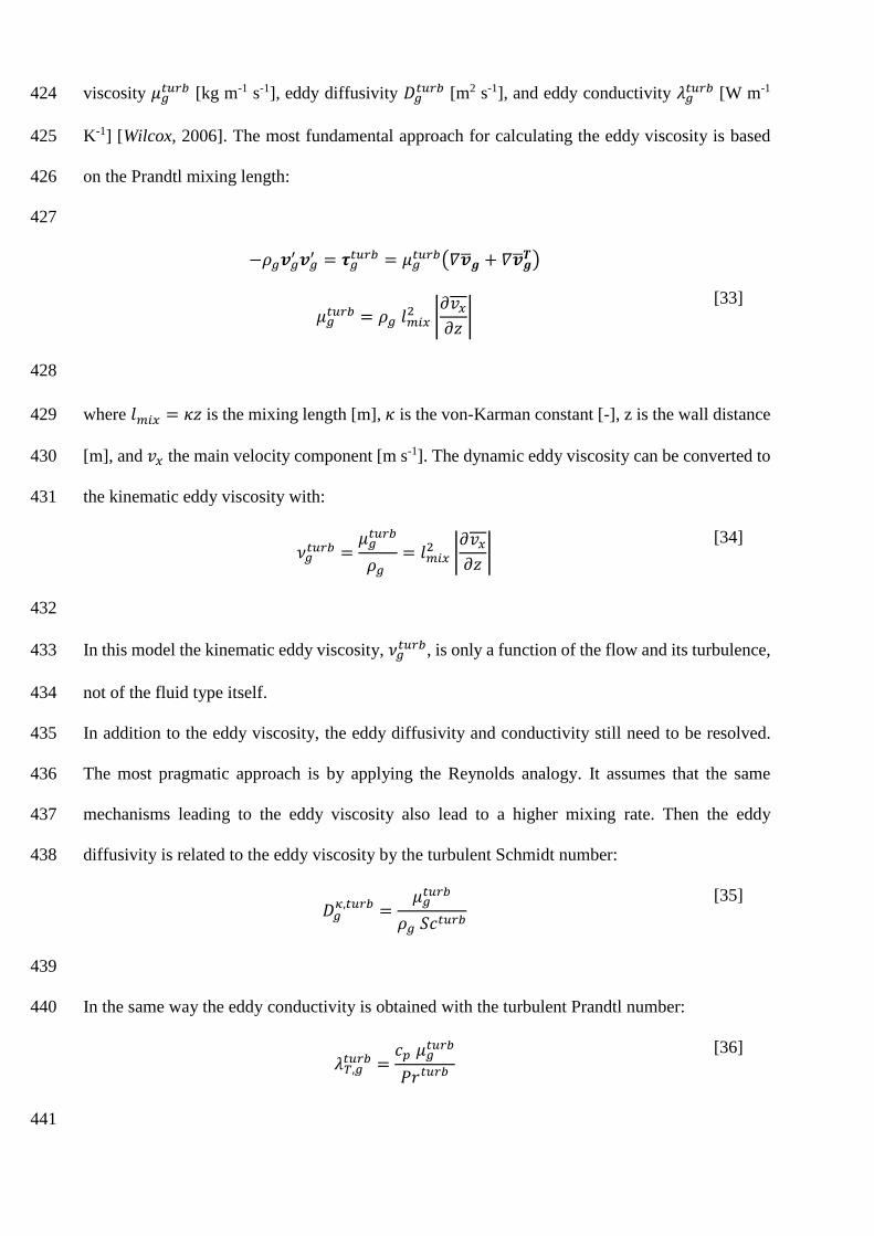
viscosity 𝜇𝑔𝑡𝑢𝑟𝑏 [kg m-1 s-1], eddy diffusivity 𝐷𝑔
𝑡𝑢𝑟𝑏 [m2 s-1], and eddy conductivity 𝜆𝑔𝑡𝑢𝑟𝑏 [W m-1 424
K-1] [Wilcox, 2006]. The most fundamental approach for calculating the eddy viscosity is based 425
on the Prandtl mixing length: 426
427
−𝜌𝑔𝒗𝑔′ 𝒗𝑔
′ = 𝝉𝑔𝑡𝑢𝑟𝑏 = 𝜇𝑔
𝑡𝑢𝑟𝑏(𝛻�̅�𝒈 + 𝛻�̅�𝒈𝑻)
𝜇𝑔𝑡𝑢𝑟𝑏 = 𝜌𝑔 𝑙𝑚𝑖𝑥
2 |𝜕𝑣𝑥𝜕𝑧|
[33]
428
where 𝑙𝑚𝑖𝑥 = 𝜅𝑧 is the mixing length [m], 𝜅 is the von-Karman constant [-], z is the wall distance 429
[m], and 𝑣𝑥 the main velocity component [m s-1]. The dynamic eddy viscosity can be converted to 430
the kinematic eddy viscosity with: 431
𝜈𝑔𝑡𝑢𝑟𝑏 =
𝜇𝑔𝑡𝑢𝑟𝑏
𝜌𝑔= 𝑙𝑚𝑖𝑥
2 |𝜕𝑣𝑥𝜕𝑧|
[34]
432
In this model the kinematic eddy viscosity, 𝜈𝑔𝑡𝑢𝑟𝑏, is only a function of the flow and its turbulence, 433
not of the fluid type itself. 434
In addition to the eddy viscosity, the eddy diffusivity and conductivity still need to be resolved. 435
The most pragmatic approach is by applying the Reynolds analogy. It assumes that the same 436
mechanisms leading to the eddy viscosity also lead to a higher mixing rate. Then the eddy 437
diffusivity is related to the eddy viscosity by the turbulent Schmidt number: 438
𝐷𝑔𝜅,𝑡𝑢𝑟𝑏 =
𝜇𝑔𝑡𝑢𝑟𝑏
𝜌𝑔 𝑆𝑐𝑡𝑢𝑟𝑏
[35]
439
In the same way the eddy conductivity is obtained with the turbulent Prandtl number: 440
𝜆𝑇,𝑔𝑡𝑢𝑟𝑏 =
𝑐𝑝 𝜇𝑔𝑡𝑢𝑟𝑏
𝑃𝑟𝑡𝑢𝑟𝑏
[36]
441
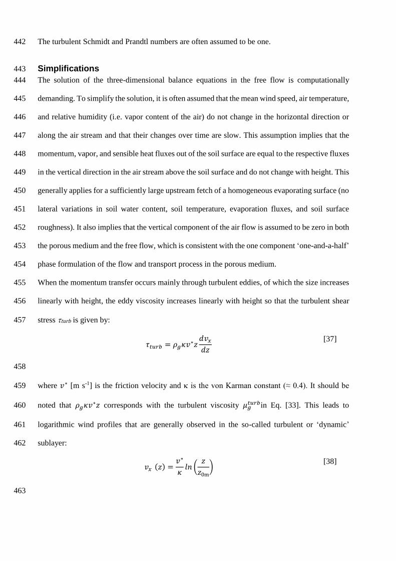
The turbulent Schmidt and Prandtl numbers are often assumed to be one. 442
Simplifications 443
The solution of the three-dimensional balance equations in the free flow is computationally 444
demanding. To simplify the solution, it is often assumed that the mean wind speed, air temperature, 445
and relative humidity (i.e. vapor content of the air) do not change in the horizontal direction or 446
along the air stream and that their changes over time are slow. This assumption implies that the 447
momentum, vapor, and sensible heat fluxes out of the soil surface are equal to the respective fluxes 448
in the vertical direction in the air stream above the soil surface and do not change with height. This 449
generally applies for a sufficiently large upstream fetch of a homogeneous evaporating surface (no 450
lateral variations in soil water content, soil temperature, evaporation fluxes, and soil surface 451
roughness). It also implies that the vertical component of the air flow is assumed to be zero in both 452
the porous medium and the free flow, which is consistent with the one component ‘one-and-a-half’ 453
phase formulation of the flow and transport process in the porous medium. 454
When the momentum transfer occurs mainly through turbulent eddies, of which the size increases 455
linearly with height, the eddy viscosity increases linearly with height so that the turbulent shear 456
stress turb is given by: 457
𝜏𝑡𝑢𝑟𝑏 = 𝜌𝑔𝜅𝑣∗𝑧𝑑𝑣𝑥𝑑𝑧
[37]
458
where 𝑣∗ [m s-1] is the friction velocity and is the von Karman constant (≈ 0.4). It should be 459
noted that 𝜌𝑔𝜅𝑣∗𝑧 corresponds with the turbulent viscosity 𝜇𝑔
𝑡𝑢𝑟𝑏in Eq. [33]. This leads to 460
logarithmic wind profiles that are generally observed in the so-called turbulent or ‘dynamic’ 461
sublayer: 462
𝑣𝑥 (𝑧) =𝑣∗
𝜅𝑙𝑛 (
𝑧
𝑧0m)
[38]
463

where 𝑧0𝑚 [m] is the momentum roughness length, which corresponds to the height above the soil 464
surface where extrapolation of Eq. [38] predicts zero velocity. Similar logarithmic profiles are 465
obtained for the air temperature and humidity. But, because of different interactions at the soil 466
surface, the temperature (z0H) and humidity (z0v) roughness lengths differ from z0m. The 467
relationship between the different roughness lengths and characteristics of the porous medium-468
free flow interface are discussed in the following section. 469
Heat and water fluxes across the soil-atmosphere interface 470
The soil-atmosphere interface represents a crucial boundary between the porous medium and the 471
free flow. In this section the coupling between transport in the atmosphere and the soil is discussed. 472
473
Coupling conditions: 474
The coupling of the two-phase porous-medium system with turbulent free flow involving the 475
Reynolds-averaged Navier-Stokes equations is based on the model presented in Mosthaf et al. 476
[2011] and revised in Mosthaf et al. [2014] and Fetzer et al. [2016]. It considers continuity of 477
fluxes and a local thermodynamic equilibrium at the interface. 478
479
Mechanical equilibrium 480
Mechanical equilibrium is defined by the continuity of normal and tangential forces. The normal 481
force acting on the interface from the free flow side is the sum of the inertia, pressure, and viscous 482
forces. The normal force from the porous-medium side of the interface contains only the pressure 483
force, since viscous forces are implicitly accounted for in Darcy’s law. Hence, the mechanical 484
equilibrium at the interface in the normal direction can be formulated as: 485
[𝒏 ∙ ({−𝜌𝑔 𝒗𝑔 𝒗𝑔 − 𝝉𝑔 − 𝝉𝑔𝑡𝑢𝑟𝑏 + 𝑝𝑔𝑰}𝒏)]
𝑓𝑓= [𝑝𝑔]
𝑝𝑚 [39]
486

The superscripts 𝑓𝑓 and 𝑝𝑚 mark the quantities at the free flow and the porous medium sides of 487
the interface in the sequel. Eq. [39] implies that the gas phase pressure may be discontinuous across 488
the interface due to the different model concepts (i.e. Navier-Stokes flow and Darcy flow) in the 489
two domains. Furthermore, in addition to considering the normal forces, the free flow requires a 490
condition for the tangential flow velocity components. When air flows over a porous surface, there 491
is a small macroscopic slip-velocity, which therefore calls the no-slip condition into question. For 492
that purpose, the Beavers-Joseph [Beavers and Joseph, 1967] or Beavers-Joseph-Saffman 493
[Saffman, 1971] condition can be employed; the latter formulation neglects the comparatively 494
small tangential velocity in the porous medium. The proportionality between the shear stresses 𝜏 495
and the slip velocity at the interface can be described as: 496
[(𝒗𝑔 −√𝑘𝑖𝛼𝐵𝐽𝜇𝑔
(𝝉𝑔 + 𝝉𝑔𝑡𝑢𝑟𝑏)𝒏) ∙ 𝒕𝑖]
𝑓𝑓
= 0, 𝑖 ∈ {1, … , 𝑑 − 1} [40]
497
Here, 𝛼𝐵𝐽 is the dimensionless Beavers-Joseph coefficient, 𝒕𝑖 is a tangential vector, and 𝑘𝑖 = 𝒕𝑖 ⋅498
(𝑘𝒕𝑖) a tangential component of the permeability tensor. The Beavers-Joseph condition was 499
originally developed for flow which is mainly tangential to the porous-medium surface and for 500
laminar single-phase flow in both the free flow and the porous medium. Its applicability for 501
turbulent flow conditions was analyzed by Hahn et al. [2002] who concluded that the slip condition 502
for laminar and turbulent flow is the same, because the flow conditions directly at the porous 503
surface can be expected to be laminar (viscous boundary layer) and velocities to be slow. 504
505
The influence of the Beavers-Joseph coefficient on the evaporation rate was analyzed in various 506
studies for different flow regimes [Baber et al., 2012; Fetzer et al., 2016]. For flow parallel to the 507
interface the evaporative fluxes are often dominated by diffusion through the boundary layer 508
normal to the interface [Haghighi et al., 2013], whereas the slip velocity promotes transport along 509
the interface. 510
511
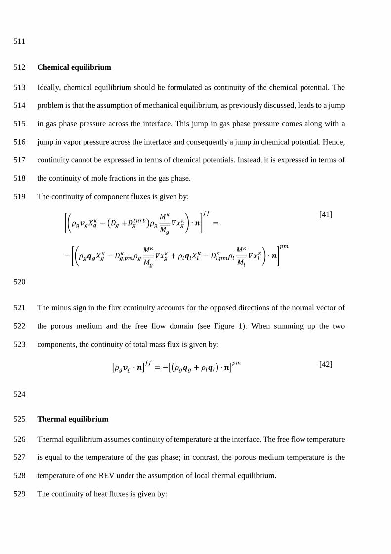
Chemical equilibrium 512
Ideally, chemical equilibrium should be formulated as continuity of the chemical potential. The 513
problem is that the assumption of mechanical equilibrium, as previously discussed, leads to a jump 514
in gas phase pressure across the interface. This jump in gas phase pressure comes along with a 515
jump in vapor pressure across the interface and consequently a jump in chemical potential. Hence, 516
continuity cannot be expressed in terms of chemical potentials. Instead, it is expressed in terms of 517
the continuity of mole fractions in the gas phase. 518
The continuity of component fluxes is given by: 519
[(𝜌𝑔𝒗𝑔𝑋𝑔𝜅 − (𝐷𝑔 +𝐷𝑔
𝑡𝑢𝑟𝑏)𝜌𝑔𝑀𝜅
𝑀𝑔𝛻𝑥𝑔
𝜅) ∙ 𝒏]
𝑓𝑓
=
−[(𝜌𝑔𝒒𝑔𝑋𝑔𝜅 − 𝐷𝑔,𝑝𝑚
𝜅 𝜌𝑔𝑀𝜅
𝑀𝑔𝛻𝑥𝑔
𝜅 + 𝜌𝑙𝒒𝑙𝑋𝑙𝜅 − 𝐷𝑙,𝑝𝑚
𝜅 𝜌𝑙𝑀𝜅
𝑀𝑙𝛻𝑥𝑙
𝜅) ∙ 𝒏]
𝑝𝑚
[41]
520
The minus sign in the flux continuity accounts for the opposed directions of the normal vector of 521
the porous medium and the free flow domain (see Figure 1). When summing up the two 522
components, the continuity of total mass flux is given by: 523
[𝜌𝑔𝒗𝑔 ∙ 𝒏]𝑓𝑓= −[(𝜌𝑔𝒒𝑔 + 𝜌𝑙𝒒𝑙) ∙ 𝒏]
𝑝𝑚 [42]
524
Thermal equilibrium 525
Thermal equilibrium assumes continuity of temperature at the interface. The free flow temperature 526
is equal to the temperature of the gas phase; in contrast, the porous medium temperature is the 527
temperature of one REV under the assumption of local thermal equilibrium. 528
The continuity of heat fluxes is given by: 529
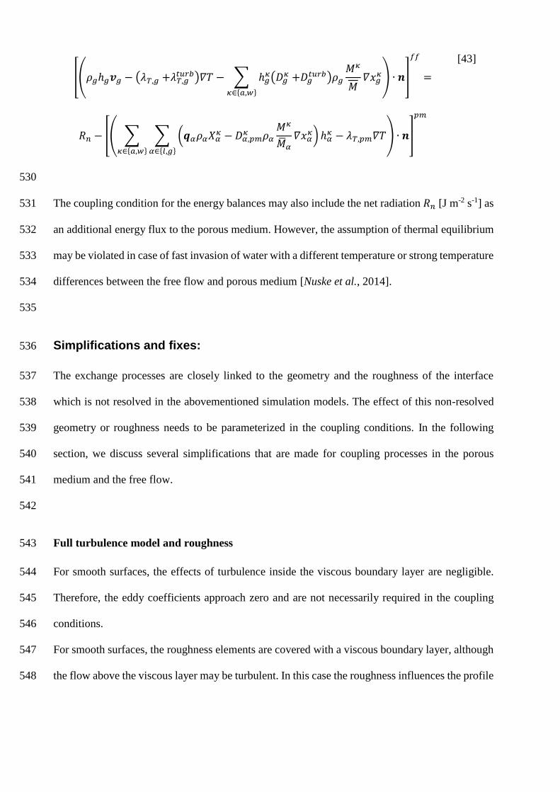
[(𝜌𝑔ℎ𝑔𝒗𝑔 − (𝜆𝑇,𝑔 +𝜆𝑇,𝑔𝑡𝑢𝑟𝑏)𝛻𝑇 − ∑ ℎ𝑔
𝜅(𝐷𝑔𝜅 +𝐷𝑔
𝑡𝑢𝑟𝑏)𝜌𝑔𝑀𝜅
𝑀𝛻𝑥𝑔
𝜅
𝜅∈{𝑎,𝑤}
) ∙ 𝒏]
𝑓𝑓
=
𝑅𝑛 − [( ∑ ∑ (𝒒𝛼𝜌𝛼𝑋𝛼𝜅 −𝐷𝛼,𝑝𝑚
𝜅 𝜌𝛼𝑀𝜅
�̅�𝛼𝛻𝑥𝛼
𝜅) ℎ𝛼𝜅 − 𝜆𝑇,𝑝𝑚𝛻𝑇
𝛼∈{𝑙,𝑔}𝜅∈{𝑎,𝑤}
) ∙ 𝒏]
𝑝𝑚
[43]
530
The coupling condition for the energy balances may also include the net radiation 𝑅𝑛 [J m-2 s-1] as 531
an additional energy flux to the porous medium. However, the assumption of thermal equilibrium 532
may be violated in case of fast invasion of water with a different temperature or strong temperature 533
differences between the free flow and porous medium [Nuske et al., 2014]. 534
535
Simplifications and fixes: 536
The exchange processes are closely linked to the geometry and the roughness of the interface 537
which is not resolved in the abovementioned simulation models. The effect of this non-resolved 538
geometry or roughness needs to be parameterized in the coupling conditions. In the following 539
section, we discuss several simplifications that are made for coupling processes in the porous 540
medium and the free flow. 541
542
Full turbulence model and roughness 543
For smooth surfaces, the effects of turbulence inside the viscous boundary layer are negligible. 544
Therefore, the eddy coefficients approach zero and are not necessarily required in the coupling 545
conditions. 546
For smooth surfaces, the roughness elements are covered with a viscous boundary layer, although 547
the flow above the viscous layer may be turbulent. In this case the roughness influences the profile 548
of the eddy coefficients in the direction normal to the surface and thus the velocity profile and the 549
viscous boundary layer thickness. Still, the coupling occurs in the viscous boundary layer. 550
For rough surfaces, the height of the roughness elements is larger than the viscous layer thickness 551
and the effects of the roughness and turbulence are important and cannot be neglected [Fetzer et 552
al., 2016]. This is accomplished by including the eddy coefficients, which are a function of 553
roughness, in the coupling conditions above. In the section on one-dimensional transfer between 554
the porous medium and the free flow, more details on the effect of roughness on the exchange 555
processes are given. 556
557
Coupled one-dimensional transfer between the soil surface and free flow: aerodynamic 558
resistances. 559
When lateral variations in wind, air temperature and humidity can be neglected, the sensible heat 560
and vapor fluxes can be described as one-dimensional fluxes that are calculated using equivalent 561
transfer resistances and differences in vapor concentrations and temperature that are measured at 562
different heights but at the same horizontal location (e.g. [Monteith and Unsworth, 1990]): 563
𝐻 = 𝑐𝑎𝑇(𝑧 = 0) − 𝑇(𝑧ref)
𝑟𝐻
[44]
𝐹𝑤 =𝜌𝑔𝑤(𝑧 = 0) − 𝜌𝑔
𝑤(𝑧ref)
𝑟𝑉
[45]
564
where H [J m-2 s-1] is the sensible heat flux, ca [J m-3 K-1] is the volumetric heat capacity of moist 565
air, zref (m) is a reference height at which wind speed, air temperature and air humidity are 566
measured or defined, Fw [kg m-2 s-1] is the water vapor flux, and rH and rV [s m -1] are the 567
aerodynamic resistance terms for vertical latent heat and vapor transfer in the air stream. Using a 568
mass and energy balance at the soil surface, the vapor and sensible heat fluxes are linked to the 569
water and vapor fluxes in the soil at the soil surface. The mass balance is given by: 570

𝐹𝑤 = [𝑞𝑙𝜌𝑙 − 𝐷g,eff𝑤 (𝑆𝑔)
𝜕𝜌𝑔𝑤
𝜕𝑧]
𝑝𝑚
[46]
571
where the first and second terms on the right hand side are the liquid water and vapor flows towards 572
the soil surface, respectively. 573
For the energy balance equation at the soil surface, the solar and long wave radiation that is 574
absorbed by and emitted from the soil surface needs to be taken into account. Calling the sum of 575
these radiation terms the net radiation, Rn [J m-2 s-1] (where positive radiation terms denote the 576
radiation that is absorbed and negative terms denote the radiation that is emitted), the energy 577
balance at the soil surface is: 578
𝐻 + ℎ𝑔𝑤𝐹𝑤 − 𝑅𝑛 = [−ℎ𝑔
𝑤𝐷g,eff𝑤 (𝑆𝑔)
𝜕𝜌𝑔𝑤
𝜕𝑧+ ℎ𝑙
𝑤𝜌𝑙𝑞𝑙 − 𝜆𝑇,𝑝𝑚𝜕𝑇
𝜕𝑧]
𝑝𝑚
[47]
579
Eqs. [44], [45], [46], [47] link the state variables, i.e. temperature and air vapor concentration, and 580
fluxes at the soil surface with state variables that are defined at the reference height in the air 581
stream. The latter may therefore be considered as Dirichlet boundary conditions for the water and 582
heat fluxes in the coupled soil-air system. This implies that the water and heat fluxes at the soil 583
surface can be derived from these prescribed state variables in the air stream and do not have to be 584
prescribed as flux boundary conditions. 585
586
Crucial parameters in Eqs. [44] and [45] are the aerodynamic resistance terms for vertical latent 587
and sensible heat transfer. They are related to the roughness of the soil surface, diffusive transfer 588
in the interfacial viscous or roughness layer, wind velocity and eddy diffusivity in the air stream, 589
and stability of the air above the heated soil surface. In the following discussion, we will consider 590
neutral stability conditions, i.e. the eddy diffusivity is not influenced by buoyancy. We refer the 591

reader to text books on meteorology (e.g. [Brutsaert, 1982; Monteith and Unsworth, 1990; 592
Shuttleworth, 2012]) for a detailed treatment of buoyancy effects. 593
In the air stream, a constant shear stress, turb [N m-2], with height is assumed. turb corresponds to 594
a momentum transfer from the air stream to the soil surface and can be expressed in terms of a 595
resistance equation similar to Eqs. [44] and [45]: 596
𝜏𝑡𝑢𝑟𝑏 = 𝜌𝑔𝑣𝑔,𝑥(𝑧ref) − 𝑣𝑔,𝑥(𝑧 = 0)
𝑟𝑀
[48]
597
where 𝑣𝑔,𝑥[m s-1] is the horizontal air velocity, and rM [s m-1] is the resistance for momentum 598
transfer between the reference height and the soil surface. rM is derived from the vertical wind 599
profile in the ‘logarithmic/dynamic’ sublayer above the roughness layer. 600
Combining Eqs. [37], [38], and [48] leads to the following expression for rM: 601
𝑟𝑀 =𝑙𝑛 (
𝑧𝑧0m
)
𝑣∗𝜅={𝑙𝑛 (
𝑧𝑧0m
)}2
𝑣𝑔,𝑥(𝑧)𝜅2
[49]
602
The momentum roughness length, 𝑧0𝑚, is a function of the kinematic viscosity of air, , the friction 603
velocity, 𝑣∗, and the height and density of the roughness elements of the soil surface. For rough 604
surfaces 𝑧0𝑚 depends only on the roughness of the surface. A prediction of 𝑧0𝑚 based on the 605
geometry of the surface roughness seems to be very uncertain and Wieringa [1993] found that the 606
relationship between 𝑧0𝑚 and the height of the surface roughness elements, d, may vary between: 607
𝑧0m =𝑑
100 𝑎𝑛𝑑 𝑧0m =
𝑑
5
[50]
608
For a small d or smooth surfaces, a viscous sublayer in which momentum transfer is dominated by 609
kinematic viscosity develops. In such a case, the velocity profiles and 𝑧0𝑚 depend on 𝑣∗ and : 610

𝑧0𝑚 = 0.135𝜈
𝑣∗
[51]
611
Whether a surface is rough or (hydrodynamically) smooth depends on the roughness Reynolds 612
number, 𝑧0+ which is defined as: 613
𝑧0+ =𝑣∗𝑧0m
𝜈
[52]
614
When 𝑧0+ > 2, the surface is considered to be rough whereas 𝑧0+ equals 0.135 for flat surfaces. It 615
should be noted that when 𝑧0𝑚 is defined by d/30, the following well-known relation for a wind 616
speed profile above a rough surface is obtained [White, 1991]: 617
𝑣𝑥(𝑧) =𝑣∗
𝜅𝑙𝑛 (
𝑧
𝑑) + 8.5𝑣∗
[53]
618
For smooth surfaces, the following relation is obtained: 619
𝑣𝑥(𝑧) =𝑣∗
𝜅𝑙𝑛 (
𝑧𝑣∗
𝜈) + 5.0𝑣∗
[54]
620
The transfer of water vapor and sensible heat in the logarithmic/dynamic sublayer is also caused 621
by turbulence and eddy diffusivity, which according to the Reynolds analogy may be considered 622
equivalent to the eddy viscosity. Therefore, a close relation between the transfer resistances for 623
momentum, sensible heat and vapor transfer may be assumed. Yet, these resistances differ from 624
each other because of the different transfer mechanisms in the viscous or roughness layer. The 625
kinematic air viscosity differs from the molecular diffusion of water and heat. Also, the roughness 626
of a bluff surface has a different effect on momentum transfer than on transfer of a scalar quantity 627
like vapor or sensible heat. For rough surfaces, momentum transfer can be considered more 628
effective or influential than vapor or heat transfer. Therefore the resistance for heat/vapor transfer 629
is larger than that for momentum transfer. As a consequence, an additional boundary resistance, 630

rB [s m-1] must be considered when relating the transfer resistances for vapor and sensible heat 631
transfer to the momentum transfer: 632
𝑟𝑉 ≈ 𝑟𝐻 = 𝑟𝑀 + 𝑟𝐵 [55]
633
The larger resistance results in a larger gradient of vapor and temperature across the viscous or 634
roughness layer; the vapor and heat roughness lengths 𝑧0𝑣 and 𝑧0𝐻 are therefore smaller than 𝑧0𝑚. 635
The similar transfer through the logarithmic/dynamic layer allows for the transfer resistance for 636
vapor and heat transport to be described using an equation similar to Eq. [49]: 637
𝑟V,H =𝑙𝑛 (
𝑧𝑧0v,H
)
𝑣∗𝜅={𝑙𝑛 (
𝑧𝑧0v,H
)}2
𝑣𝑔,𝑥(𝑧)𝜅2
[56]
638
This equation may be rewritten in terms of rm and rB as: 639
𝑟V,H = 𝑟𝑀 + 𝑟𝐵 =𝑙𝑛 [
𝑧𝑧0v,H
]
𝜅𝑣∗=𝑙𝑛 [
𝑧𝑧0m
]
𝜅𝑣∗+𝑙𝑛 [
𝑧0m𝑧0v,H
]
𝜅𝑣∗=𝑙𝑛 [
𝑧𝑧0m
]2
𝜅2𝑣𝑔,𝑥(𝑧)+𝑙𝑛 [
𝑧𝑧0m
] 𝑙𝑛 [𝑧0m𝑧0v,H
]
𝜅2𝑣𝑔,𝑥(𝑧)
[57]
640
A number of equations that relate 𝑧0𝑣,𝐻 with 𝑧0𝑚 and 𝑣∗ have been proposed (see for instance 641
Yang et al. [2008]). Brutsaert [1982] developed the following relation between 𝑧0𝑚 and 𝑧0𝑣,𝐻: 642
𝑧0v,H𝑧0m
= 7.4𝑒𝑥𝑝 [−2.46 (𝑣∗𝑧0m𝜈
)0.25
] = 7.4𝑒𝑥𝑝 [−2.46(𝑘𝑣𝑔,𝑥(𝑧)𝑧0m
𝑙𝑛 (𝑧𝑧0m
) 𝜈)
0.25
]
[58]
643
In Figure 2, the calculated resistances using Eq [49], [50], [57], and [58] for different surface 644
roughness lengths, d and two wind velocities, 𝑣𝑔,𝑥, at 2m height above the soil surface are shown. 645
According to these calculations, the total resistance (rH) decreases with increasing roughness. This 646
can be attributed to the decreasing transfer resistance in the logarithmic/dynamic sublayer with 647
increasing roughness of the soil surface. However, the difference between transfer resistance for 648
momentum transfer, rM, and heat/vapor transfer, rV,H (i.e. rB,) increases with increasing roughness. 649
For heat/vapor transfer, the effect of larger turbulent diffusivity in the logarithmic/dynamic layer 650
above a rougher soil surface is counteracted by a longer diffusive pathway through a thicker 651
roughness layer. As a consequence, the decrease of the resistance for heat/vapor transfer with 652
increasing surface roughness is less prevalent than the decrease of momentum transfer resistance 653
(Figure 2). 654
It should be noted that the transfer resistances described above are based on the assumption of a 655
bluff surface with a no-slip boundary condition. As described before, slip conditions may apply at 656
the surface of a porous medium, which can be accounted for by Beavers-Joseph interface boundary 657
conditions. One way to represent these effects is to define a displacement height, similar to what 658
is used to describe momentum, heat, and vapor transfer between vegetated surfaces and the 659
atmosphere. However, this displacement height should be negative. We are at this moment, not 660
aware of any studies that specify such displacement heights for air flow over rough dry porous 661
media. 662
663
Semi-coupled porous medium and free flow using potential evaporation rates and soil 664
surface resistances for drying porous medium. 665
In the sections above, we described how water flow and heat transport in the porous medium and 666
the free flow are coupled at the interface. However, this coupling is often relaxed by specifying or 667
defining state variables a-priori at the interface. When the vapor pressure at the interface is defined 668
to be the saturated vapor pressure, the water flux from the interface into the free flow is:: 669
𝐹w,pot =𝜌𝑔,𝑠𝑎𝑡𝑤 (𝑧 = 0) − 𝜌𝑔
𝑤(𝑧𝑟𝑒𝑓)
𝑟𝑉
[59]
where Fw,pot is the so-called potential evaporation, which is calculated without considering the 670
porous medium. It represents the ‘demand’ for water by the atmosphere and can be used as a flux 671
boundary condition in the porous medium as long as the flow in the porous medium can ‘supply’ 672
the demand. The saturated vapor concentration at the soil surface depends on the soil surface 673
temperature, which is derived from solving the surface energy balance (Eq. [47]). _ENREF_1 674
An additional soil transfer resistance, rs [s m-1] was introduced to account for a reduction in 675
evaporation when the soil surface dries out and the vapor pressure becomes smaller than the 676
saturated vapor pressure: 677
𝐹𝑤 =𝜌𝑔,𝑠𝑎𝑡𝑤 (𝑧 = 𝑧𝑒𝑣𝑎𝑝) − 𝜌𝑔
𝑤(𝑧𝑟𝑒𝑓)
𝑟𝑉 + 𝑟𝑠(𝜃𝑙,𝑡𝑜𝑝)= 𝛽(𝜃𝑙,𝑡𝑜𝑝)𝐹𝑤,𝑝𝑜𝑡
[60]
678
where zevap is the depth where evaporation takes place (i.e. where air is assumed to be saturated 679
with vapor) and l,top is the water content of the ‘top soil layer’. However, neither zevap nor the 680
thickness of the top soil layer are explicitly defined or simulated. The soil transfer resistance, rs, is 681
a function of the water content in the top soil layer whereas rv depends on the free flow conditions. 682
Water transport in the porous medium and into the atmosphere are hence semi-coupled in this 683
approach. The factor represents the ratio of the aerodynamic resistance to the sum of the soil and 684
aerodynamic resistance. This approach is often used in large scale simulation models to describe 685
the reduction of evaporation from drying bare soil compared with the potential evaporation from 686
wet soil [Tang and Riley, 2013a]. 687
Kondo et al. [1990], Mahfouf and Noilhan [1991], and Vandegriend and Owe [1994] used a soil 688
transfer resistance term that increases with decreasing surface soil water content to account for the 689
additional resistance for diffusive vapor transfer when the evaporative surface recedes into the soil 690
profile and Tang and Riley [2013a] derived a model for the soil transfer resistance based on the 691
vapor diffusivity and liquid water hydraulic conductivity. Experimentally derived soil transfer 692
resistances were smaller than expected, considering the depth of the evaporation surface and the 693
vapor diffusion coefficient. The smaller resistances were attributed to turbulent eddies that 694
propagate into the porous medium and generate upward and downward movement of air and hence 695
an extra opportunity for mixing with incoming air in the upper soil layer [Farrell et al., 1966; 696
Ishihara et al., 1992; Kimball and Lemon, 1971; Scotter and Raats, 1969]. It should be noted that 697
Assouline et al. [2013] found that the evaporation flux calculated using Ficks’ Law and the depth 698
of the evaporation front (i.e. zevap) underestimated the evaporation rate; however turbulent mixing 699
was not recognized in this case as a potentially relevant process. Additional turbulent mixing leads 700
to an additional dispersive flux of gases in the upper soil layer and has been shown to be of 701
importance for the flux of vapor and trace gases from soil [Baldocchi and Meyers, 1991; Maier et 702
al., 2012; Poulsen and Moldrup, 2006] and soil covered with mulches [Fuchs and Hadas, 2011]. 703
The parameterization of this additional mixing due to turbulence in the top soil is not well known 704
and debated. 705
A second reason for a decrease in evaporation rate from a drying surface is the spatial variation of 706
the vapor pressure at the soil surface at the microscopic scale. When the lateral distance between 707
evaporating water surfaces in pores at the soil surface becomes too large, the reduction of the 708
evaporating water surface when the soil surface dries out cannot be compensated by an increased 709
lateral diffusion of vapor through the viscous or roughness layer [Haghighi et al., 2013; 710
Shahraeeni et al., 2012; Suzuki and Maeda, 1968]. In this case, vapor transfer through the viscous 711
or roughness layer rather than vapor transfer within the porous medium is the limiting factor. If 712
this effect is also accounted for by an additional resistance term, experimental results of 713
Shahraeeni et al. [2012] suggest that this resistance term increases with decreasing surface soil 714
water content, that it is larger in soils with larger pores, and that the ratio of this resistance term to 715
the resistance for vapor transport from a saturated soil surface increases with increasing wind 716
velocity. It should be noted that a similar relation with wind speed is observed for the ratio of rB/rM 717
(see Figure 2). 718
Soil transfer resistances have been introduced in soil evaporation models. However, using an 719
additional transfer resistance in a model that explicitly considers diffusive vapor transfer in the 720
soil surface layer (e.g. Saito et al. [2006]) leads to a double counting of the transfer resistance 721
through the soil surface layer and therefore a too strong and rapid decrease in the actual 722
evaporation rate from the soil surface. 723
724
Threshold formulation of boundary conditions. 725
In this approach, water transfer between the porous medium and the free flow is either fully 726
controlled by free flow conditions or by water transport in the porous medium. When the free flow 727
controls the transfer, the potential evaporation is used as a flux boundary condition for water flow 728
in the porous medium. When the porous medium controls the flux, a constant water pressure or 729
water content at the surface of the porous medium is defined and the water flux towards the soil 730
surface is calculated by solving the flow equations in the porous medium for a Dirichlet boundary 731
condition. This approach is used in soil models that solve the Richards equation, e.g. Hydrus 1D 732
[Simunek et al., 2008]. There are no exact guidelines to define the critical pressure head, crit, 733
which is kept constant at the porous medium surface. As a rule of thumb, crit should correspond 734
with a pressure head for which the hydraulic conductivity and capacity of the porous medium 735
(d/d) become very small so that a smaller crit would hardly influence simulated water contents 736
and water fluxes towards the soil surface. As will be shown in some simulation examples in the 737
accompanying paper, simulated water fluxes are not so sensitive to the exact choice of this critical 738
pressure head. 739
740
Summary and Conclusions: 741
This work presented an overview of concepts with different complexity that can be used to describe 742
the transfer of water and energy from a porous medium into free flow. We identified how the 743
different approaches are related and which simplifications are used. The most comprehensive 744
description of processes considered multi-dimensional flow of liquid and gas phases and transport 745

of dry air and water components in the porous medium that was coupled consistently 746
acknowledging mechanical, chemical and thermal equilibrium at the interface to a free flow in the 747
gas phase and transport of vapor and heat above the porous medium. Since the direction of the free 748
flow is generally different from the main direction of the flow and transport processes in the porous 749
medium, this comprehensive approach implies a multi-dimensional description of the flow and 750
transport processes. 751
However, for homogeneous soil surfaces of a sufficiently large fetch, lateral variations in state 752
variables in the free flow become very small. This leads to a first simplification from a multi- to a 753
one dimensional description of the flow and transport processes in which only the vertical 754
components of flow and transport (in the porous medium) are considered and the vertical 755
components of the gas flow in both the porous medium and the free flow are neglected. This 756
implies that in the porous medium transport in the gas phase happens by diffusion only (i.e. air 757
flow is neglected). This assumption allows to couple the water and heat fluxes in the porous 758
medium and in the free-flow at the porous medium interface using transfer resistances that 759
calculate fluxes from states at the soil/free-flow interface and at a defined height in the free-flow. 760
A second simplification assumes that vapor transport in the porous medium can be neglected 761
leading to the one component one phase or so-called Richards equation. This simplification 762
decouples water from heat fluxes in the porous medium. At the porous-medium free flow interface, 763
the heat balance equation is solved to determine the water flux at the interface. This balance is 764
solved assuming that the vapor concentration at the soil surface is equal to the saturated vapor 765
concentration so that the heat balance equation is in fact decoupled from the water flow equation 766
in the porous medium. The water fluxes that are derived from this heat balance apply therefore 767
only when the soil surface is sufficiently wet. 768
The third set of simplifications is related to the description of the interactions or the coupling of 769
the water flow in the porous medium, the interface heat balance, and the evaporation from the 770
interface. In a first approach the transfer between the porous medium and free flow is described 771
by threshold boundary conditions that use prescribed fluxes derived from a surface energy balance 772
until a critical threshold water pressure head is reached at the porous medium surface. This so-773
called Richards equation with threshold boundary conditions is widely used in soil water balance 774
models. During periods when the pressure head at the surface equals the critical pressure head, the 775
dynamics of the evaporation fluxes are completely defined by the hydraulic properties of the 776
porous medium and the water distribution in the porous medium but are decoupled from the 777
dynamics of the evaporative forcing: radiation, free flow velocity, relative humidity and 778
temperature. A second approach, which is often used in large scale simulation models, combines 779
the diurnal dynamics of the evaporation of a wet surface with a soil surface resistance depending 780
on the soil water content and represents a semi-coupling between the dynamics of the evaporative 781
forcing and the flow process in the porous medium. 782
Finally, there are processes that are not represented or resolved in the comprehensive process 783
description that we presented. These processes are parameterized in the vapor transport description 784
in the porous medium and in the transfer resistances for momentum, heat and vapor transfer 785
between the porous medium and the free flow. . Processes like turbulent diffusion and 786
enhancement of thermal vapor diffusion by thermal non-equilibrium within the porous medium 787
are parameterized in the vapor transport. Non-equilibria (thermal and chemical) can be included 788
in the models by adding additional equations that describe the rate with which an equilibrium is 789
reached, typically first-order rates [Smits et al., 2011]. The rate coefficients are in essence 790
additional empirical parameters that need to be estimated, for example by inverse modeling. Since 791
the surface roughness is not represented in the continuum equations, the effect of roughness on the 792
exchange processes needs to be parameterized in the transfer resistances. Because the small scale 793
mechanisms that control the exchange processes at a rough interface differ for momentum vs heat 794
and vapor exchanges, the parameterizations of the respective transfer resistances differ. However, 795
these parameterizations have been derived mainly for bluff surfaces. Therefore, the effect of 796
vertical (turbulent pumping) and lateral gas flow in the surface layer of the porous medium, which 797
may be important in highly porous mulches, aggregated soils, and dry soils, is not accounted for. 798
Based on this summary, we conclude that the description of evaporation processes in systems 799
where an important lateral variation in fluxes and states can be expected would require a 800
multidimensional representation of the processes in both the porous medium and the free flow. 801
Although this seems at first sight trivial, it is in fact not generally applied. For instance, several 802
studies that investigated the effect of soil heterogeneity on soil water fluxes use a multidimensional 803
description of the flow process in the porous medium but describe the transfer from the soil surface 804
into the atmosphere using transfer resistances that presume laterally homogeneous state variables 805
in the free flow. 806
The consideration of the vapor transport in the porous medium and its parameterization due to 807
non-represented processes or its indirect representation in transfer resistances between the porous 808
medium and the free flow is another important difference between the presented model concepts. 809
Under which conditions these differences lead to important differences in simulated evaporation 810
needs to be further investigated. 811
These conclusions are the starting point of accompanying paper in which we will evaluate the 812
impact of lateral variability and the representation of vapor transport in the porous medium on 813
evaporation simulations. 814
815

Acknowledgements: 816
817
The authors would like to acknowledge the German Science Foundation, DFG. This work is a 818
contribution of the DFG research unit “Multi-Scale Interfaces in Unsaturated Soil” (MUSIS; FOR 819
1083) and the DFG International Research Training Group NUPUS and the National Science 820
Foundation (NSF EAR-1447533). 821
The authors would like to thank the editor and the anonymous reviewers for their insightful 822
comments and suggestions that have contributed to improve this paper. 823
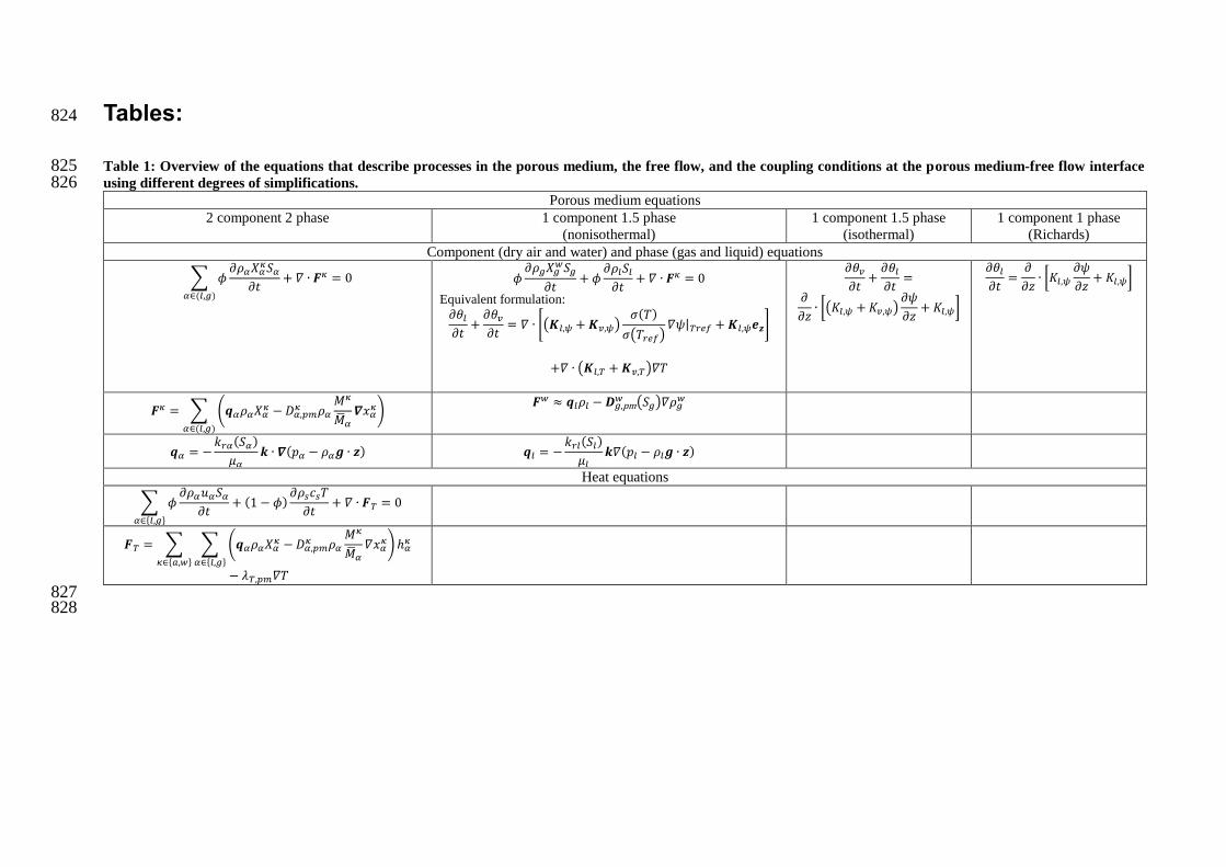
Tables: 824
Table 1: Overview of the equations that describe processes in the porous medium, the free flow, and the coupling conditions at the porous medium-free flow interface 825 using different degrees of simplifications. 826
Porous medium equations
2 component 2 phase 1 component 1.5 phase
(nonisothermal)
1 component 1.5 phase
(isothermal)
1 component 1 phase
(Richards)
Component (dry air and water) and phase (gas and liquid) equations
∑ 𝜙𝜕𝜌𝛼𝑋𝛼
𝜅𝑆𝛼𝜕𝑡
+ 𝛻 ∙ 𝑭𝜅 = 0
𝛼∈(𝑙,𝑔)
𝜙𝜕𝜌𝑔𝑋𝑔
𝑤𝑆𝑔
𝜕𝑡+ 𝜙
𝜕𝜌𝑙𝑆𝑙𝜕𝑡
+ 𝛻 ∙ 𝑭𝜅 = 0
Equivalent formulation:
𝜕𝜃𝑙𝜕𝑡+𝜕𝜃𝑣𝜕𝑡
= 𝛻 ∙ [(𝑲𝑙,𝜓 +𝑲𝑣,𝜓)𝜎(𝑇)
𝜎(𝑇𝑟𝑒𝑓)𝛻𝜓|𝑇𝑟𝑒𝑓 +𝑲𝑙,𝜓𝒆𝒛]
+𝛻 ∙ (𝑲𝑙,𝑇 +𝑲𝑣,𝑇)𝛻𝑇
𝜕𝜃𝑣𝜕𝑡
+𝜕𝜃𝑙𝜕𝑡
=
𝜕
𝜕𝑧∙ [(𝐾𝑙,𝜓 +𝐾𝑣,𝜓)
𝜕𝜓
𝜕𝑧+ 𝐾𝑙,𝜓]
𝜕𝜃𝑙𝜕𝑡
=𝜕
𝜕𝑧∙ [𝐾𝑙,𝜓
𝜕𝜓
𝜕𝑧+ 𝐾𝑙,𝜓]
𝑭𝜅 = ∑ (𝒒𝛼𝜌𝛼𝑋𝛼𝜅 −𝐷𝛼,𝑝𝑚
𝜅 𝜌𝛼𝑀𝜅
�̅�𝛼𝜵𝑥𝛼
𝜅)
𝛼∈(𝑙,𝑔)
𝑭𝑤 ≈ 𝒒𝑙𝜌𝑙 − 𝑫𝑔,pm
𝑤 (𝑆𝑔)𝛻𝜌𝑔𝑤
𝒒𝛼 = −𝑘𝑟𝛼(𝑆𝛼)
𝜇𝛼𝒌 ∙ 𝜵(𝑝𝛼 − 𝜌𝛼𝒈 ∙ 𝒛) 𝒒𝑙 = −
𝑘𝑟𝑙(𝑆𝑙)
𝜇𝑙𝒌𝛻(𝑝𝑙 − 𝜌𝑙𝒈 ∙ 𝒛)
Heat equations
∑ 𝜙𝜕𝜌𝛼𝑢𝛼𝑆𝛼𝜕𝑡
+ (1 − 𝜙)𝜕𝜌𝑠𝑐𝑠𝑇
𝜕𝑡+ 𝛻 ∙ 𝑭𝑇 = 0
𝛼∈{𝑙,𝑔}
𝑭𝑇 = ∑ ∑ (𝒒𝛼𝜌𝛼𝑋𝛼𝜅 −𝐷𝛼,𝑝𝑚
𝜅 𝜌𝛼𝑀𝜅
�̅�𝛼𝛻𝑥𝛼
𝜅)ℎ𝛼𝜅
𝛼∈{𝑙,𝑔}𝜅∈{𝑎,𝑤}
− 𝜆𝑇,𝑝𝑚𝛻𝑇
827 828

Free flow equations
Mass balance, Reynolds averaged Navier Stokes, component and energy balance 1-D steady state 𝜕𝜌𝑔
𝜕𝑡+ 𝛻 ∙ [𝜌𝑔 𝒗𝑔] = 0
𝜕(𝜌𝑔𝒗𝑔)
𝜕𝑡+ 𝛻 ∙ [𝜌𝑔 𝒗𝑔 𝒗𝑔 + 𝑝𝑔̅̅ ̅𝑰 − (𝜇𝒈
𝒕𝒖𝒓𝒃 + 𝜇𝑔 )(𝛻�̅�𝒈 + 𝛻�̅�𝒈𝑻)] − 𝜌𝑔𝒈 = 0
𝑑
𝑑𝑧𝜇𝒈𝒕𝒖𝒓𝒃
𝑑𝑣𝑔,𝑥
𝑑𝑧= 0
𝜕𝜌𝑔𝑋𝑔𝜅
𝜕𝑡+ 𝛻 ∙ (𝜌𝑔 𝒗𝑔𝑋𝑔
𝜅 − (𝐷𝑔𝑡𝑢𝑟𝑏 + 𝐷𝑔
𝜅 )𝜌𝑔𝑀𝜅
𝑀𝑔𝛻𝑥𝑔
𝜅) = 0 𝑑
𝑑𝑧𝐷𝒈𝒕𝒖𝒓𝒃
𝑑𝜌𝑔𝑤
𝑑𝑧= 0
𝜕𝜌𝑔 𝑢𝑔
𝜕𝑡+ 𝛻 ∙ (𝜌𝑔 𝒗𝑔 ℎ𝑔 − (𝜆𝑇,𝑔
𝑡𝑢𝑟𝑏 + 𝜆𝑇,𝑔)𝛻𝑇 − ∑ ℎ𝑔𝜅(𝐷𝑔
𝑡𝑢𝑟𝑏 + 𝐷𝑔𝜅,)𝜌𝑔
𝑀𝜅
𝑀𝑔𝛻𝑥𝑔
𝜅
𝜅∈{𝑎,𝑤}
) = 0
𝑑
𝑑𝑧𝜆𝑇,𝑔𝑡𝑢𝑟𝑏
𝑑𝑇
𝑑𝑧= 0
829
830
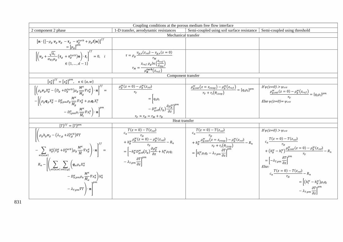
Coupling conditions at the porous medium free flow interface
2 component 2 phase 1-D transfer, aerodynamic resistances Semi-coupled using soil surface resistance Semi-coupled using threshold
Mechanical transfer
[𝒏 ∙ ({−𝜌𝑔 𝒗𝑔 𝒗𝑔 − 𝝉𝑔 − 𝝉𝑔𝑡𝑢𝑟𝑏 + 𝑝𝑔𝑰}𝒏)]
𝑓𝑓
= [𝑝𝑔]𝑝𝑚
[(𝒗𝑔 +√𝑘𝑖𝛼𝐵𝐽𝜇𝑔
(𝝉𝑔 + 𝝉𝑔𝑡𝑢𝑟𝑏)𝒏) ∙ 𝒕𝑖]
𝑓𝑓
= 0, 𝑖
∈ {1,… , 𝑑 − 1}
𝜏 = 𝜌𝑔𝑣𝑔,𝑥(𝑧ref) − 𝑣𝑔,𝑥(𝑧 = 0)
𝑟𝑀
𝑟𝑀 =𝑧𝑟𝑒𝑓 𝜌𝑔𝑙𝑛 (
𝑧𝑟𝑒𝑓𝑧0m
)
𝜇𝒈𝒕𝒖𝒓𝒃(𝑧𝑟𝑒𝑓)
Component transfer
[𝑥𝑔𝜅]𝑓𝑓= [𝑥𝑔
𝜅]𝑝𝑚, 𝜅 ∈ {𝑎, 𝑤}
[(𝜌𝑔𝒗𝑔𝑋𝑔𝜅 − (𝐷𝑔 +𝐷𝑔
𝑡𝑢𝑟𝑏)𝜌𝑔𝑀𝜅
𝑀𝑔𝛻𝑥𝑔
𝜅) ∙ 𝒏]
𝑓𝑓
=
−[(𝜌𝑔𝒒𝑔𝑋𝑔𝜅 − 𝐷𝑔,𝑝𝑚
𝜅 𝜌𝑔𝑀𝜅
𝑀𝑔𝛻𝑥𝑔
𝜅 + 𝜌𝑙𝒒𝑙𝑋𝑙𝜅
− 𝐷𝑙,𝑝𝑚𝜅 𝜌𝑙
𝑀𝜅
𝑀𝑙𝛻𝑥𝑙
𝜅) ∙ 𝒏]
𝑝𝑚
𝜌𝑔𝑤(𝑧 = 0) − 𝜌𝑔
𝑤(𝑧ref)
𝑟𝑉
= [𝑞𝑙𝜌𝑙
−𝐷g,eff𝑤 (𝑆𝑔)
𝜕𝜌𝑔𝑤
𝜕𝑧]
𝑝𝑚
𝑟𝑉 ≈ 𝑟𝐻 = 𝑟𝑀 + 𝑟𝐵
𝜌𝑔,𝑠𝑎𝑡𝑤 (𝑧 = 𝑧𝑒𝑣𝑎𝑝) − 𝜌𝑔
𝑤(𝑧𝑟𝑒𝑓)
𝑟𝑉 + 𝑟𝑠(𝜃𝑙,𝑡𝑜𝑝)= [𝑞𝑙𝜌𝑙]
𝑝𝑚 If (z=0) > crit
𝜌𝑔,𝑠𝑎𝑡𝑤 (𝑧 = 0) − 𝜌𝑔
𝑤(𝑧𝑟𝑒𝑓)
𝑟𝑉= [𝑞𝑙𝜌𝑙]
𝑝𝑚
Else (z=0)=crit
Heat transfer [𝑇]𝑓𝑓 = [𝑇]𝑝𝑚
[(𝜌𝑔ℎ𝑔𝒗𝑔 − (𝜆𝑇,𝑔 +𝜆𝑇,𝑔𝑡𝑢𝑟𝑏)𝛻𝑇
− ∑ ℎ𝑔𝜅(𝐷𝑔
𝜅 +𝐷𝑔𝑡𝑢𝑟𝑏)𝜌𝑔
𝑀𝜅
𝑀𝛻𝑥𝑔
𝜅
𝜅∈{𝑎,𝑤}
) ∙ 𝒏]
𝑓𝑓
=
𝑅𝑛 − [( ∑ ∑ (𝒒𝛼𝜌𝛼𝑋𝛼𝜅
𝛼∈{𝑙,𝑔}𝜅∈{𝑎,𝑤}
− 𝐷𝛼,𝑝𝑚𝜅 𝜌𝛼
𝑀𝜅
�̅�𝛼𝛻𝑥𝛼
𝜅)ℎ𝛼𝜅
− 𝜆𝑇,𝑝𝑚𝛻𝑇) ∙ 𝒏]
𝑝𝑚
𝑐𝑎𝑇(𝑧 = 0) − 𝑇(𝑧ref)
𝑟𝐻
+ ℎ𝑔𝑤𝜌𝑔𝑤(𝑧 = 0) − 𝜌𝑔
𝑤(𝑧ref)
𝑟𝑉− 𝑅𝑛
= [−ℎ𝑔𝑤𝐷g,eff
𝑤 (𝑆𝑔)𝜕𝜌𝑔
𝑤
𝜕𝑧+ ℎ𝑙
𝑤𝜌𝑙𝑞𝑙
− 𝜆𝑇,𝑝𝑚𝜕𝑇
𝜕𝑧]
𝑝𝑚
𝑐𝑎𝑇(𝑧 = 0) − 𝑇(𝑧ref)
𝑟𝐻
+ ℎ𝑔𝑤𝜌𝑔,𝑠𝑎𝑡𝑤 (𝑧 = 𝑧𝑒𝑣𝑎𝑝) − 𝜌𝑔
𝑤(𝑧ref)
𝑟𝑉 + 𝑟𝑠(𝜃𝑙,𝑡𝑜𝑝)− 𝑅𝑛
= [ℎ𝑙𝑤𝜌𝑙𝑞𝑙 − 𝜆𝑇,𝑝𝑚
𝜕𝑇
𝜕𝑧]𝑝𝑚
If (z=0) > crit
𝑐𝑎𝑇(𝑧 = 0) − 𝑇(𝑧ref)
𝑟𝐻
+ (ℎ𝑔𝑤 − ℎ𝑙
𝑤)𝜌𝑔,𝑠𝑎𝑡𝑤 (𝑧 = 0) − 𝜌𝑔
𝑤(𝑧ref)
𝑟𝑉− 𝑅𝑛
= [−𝜆𝑇,𝑝𝑚𝜕𝑇
𝜕𝑧]𝑝𝑚
Else:
𝑐𝑎𝑇(𝑧 = 0) − 𝑇(𝑧ref)
𝑟𝐻− 𝑅𝑛
= [(ℎ𝑙𝑤 − ℎ𝑔
𝑤)𝜌𝑙𝑞𝑙
− 𝜆𝑇,𝑝𝑚𝜕𝑇
𝜕𝑧]𝑝𝑚
831

43
Figures: 832
833
Figure 1: Sketch of the two-domain concept and the notation of the normal vectors (after Mosthaf et al. 834
835

44
836
Figure 2: Aerodynamic resistances for sensible heat (and vapor) (rH) and momentum transfer (rm) through 837 the boundary layer as function of the surface roughness length, d, for two different wind speeds, vg,x at 2 m 838 height. rB represents the additional resistance for heat transfer compared with momentum transfer. 839 840
841

45
References: 842
843
Assouline, S., K. Narkis, and D. Or (2010), Evaporation from partially covered water surfaces, 844
Water Resour. Res., 46, W10539 doi: 10.1029/2010wr009121. 845
Assouline, S., S. W. Tyler, J. S. Selker, I. Lunati, C. W. Higgins, and M. B. Parlange (2013), 846
Evaporation from a shallow water table: Diurnal dynamics of water and heat at the surface of 847
drying sand, Water Resour. Res., 49(7), 4022-4034, doi: 10.1002/wrcr.20293. 848
Baber, K., K. Mosthaf, B. Flemisch, R. Helmig, S. Müthing, and B. Wohlmuth (2012), 849
Numerical scheme for coupling two-phase compositional porous-media flow and one-phase 850
compositional free flow, IMA Journal of Applied Mathematics, 77 (6), 887-909 851
Bachmann, J., R. Horton, and R. R. van der Ploeg (2001), Isothermal and nonisothermal 852
evaporation from four sandy soils of different water repellency, Soil Sci. Soc. Am. J., 65(6), 853
1599-1607. 854
Bachmann, J., R. Horton, S. A. Grant, and R. R. van der Ploeg (2002), Temperature dependence 855
of water retention curves for wettable and water-repellent soils, Soil Sci. Soc. Am. J., 66(1), 44-856
52. 857
Baldocchi, D. D., and T. P. Meyers (1991), Trace gas-exchange above the floor of a deciduous 858
forest .1. Evaporation and co2 efflux, J. Geophys. Res.-Atmos., 96(D4), 7271-7285, doi: 859
10.1029/91jd00269. 860
Beavers, G. S., and D. D. Joseph (1967), Boundary conditions at a naturally permeable wall, J. 861
Fluid Mech., 30, 197-&, doi: 10.1017/s0022112067001375. 862
Bechtold, M., J. Vanderborght, L. Weihermuller, M. Herbst, T. Gunther, O. Ippisch, R. Kasteel, 863
and H. Vereecken (2012), Upward transport in a three-dimensional heterogeneous laboratory 864
soil under evaporation conditions, Vadose Zone J., 11(2), doi: 10.2136/vzj2011.0066. 865
Benet, J. C., and P. Jouanna (1982), Phenomenological relation of phase-change of water in a 866
porous-medium - experimental-verification and measurement of the phenomenological 867
coefficient, Int. J. Heat Mass Transfer, 25(11), 1747-1754, doi: 10.1016/0017-9310(82)90154-868
5. 869
Bird, R. B., W. E. Stewart, and E. N. Lightfoot (2007), Transport phenomena, 905 pp., Wiley, 870
New York. 871
Boussinesq, J. (1872), Essai sur la théorie des eaux courantes, Memoires Acad. des Sciences, 872
23(1). 873
Bristow, K. L., and R. Horton (1996), Modeling the impact of partial surface mulch on soil heat 874
and water flow, Theor. Appl. Climatol., 54(1-2), 85-98, doi: 10.1007/bf00863561. 875
Brooks, R. H., and A. T. Corey (1964), Hydraulic properties of porous media.Rep., Fort Collins, 876
Colorado. 877
Brutsaert, W. (1982), Evaporation into the atmosphere. Theory, history, and applications, 299 878
pp., D.Reidel Publishing Company, Dordrecht. 879
Brutsaert, W., and S. L. Yu (1968), Mass transfer aspects of pan evaporation, J. Appl. Meteorol., 880
7(4), 563-566. 881
Campbell, G. S. (1985), Soil physics with basic, Elsevier, New York. 882
Campbell, G. S., J. D. Jungbauer, W. R. Bidlake, and R. D. Hungerford (1994), Predicting the 883
effect of temperature on soil thermal-conductivity, Soil Sci., 158(5), 307-313. 884
Cass, A., G. S. Campbell, and T. L. Jones (1984), Enhancement of thermal water-vapor 885
diffusion in soil, Soil Sci. Soc. Am. J., 48(1), 25-32. 886
Chammari, A., B. Naon, F. Cherblanc, B. Cousin, and J. C. Benet (2008), Interpreting the 887
drying kinetics of a soil using a macroscopic thermodynamic nonequilibrium of water between 888
the liquid and vapor phase, Dry. Technol., 26(7), 836-843, doi: 10.1080/07373930802135998. 889

46
Chung, S. O., and R. Horton (1987), Soil heat and water-flow with a partial surface mulch, 890
Water Resour. Res., 23(12), 2175-2186, doi: 10.1029/WR023i012p02175. 891
Cote, J., and J. M. Konrad (2005), A generalized thermal conductivity model for soils and 892
construction materials, Can. Geotech. J., 42(2), 443-458. 893
Cote, J., and J. M. Konrad (2009), Assessment of structure effects on the thermal conductivity 894
of two-phase porous geomaterials, Int. J. Heat Mass Transfer, 52(3-4), 796-804, doi: 895
10.1016/j.ijheatmasstransfer.2008.07.037. 896
Davis, D. D., R. Horton, J. L. Heitman, and T. S. Ren (2014), An experimental study of coupled 897
heat and water transfer in wettable and artificially hydrophobized soils, Soil Sci. Soc. Am. J., 898
78(1), 125-132, doi: 10.2136/sssaj2013.05.0182. 899
de Vries, D. A. (1958), Simultaneous transfer of heat and moisture in porous media, 900
Transactions, American Geophysical Union, 39(5), 909-916. 901
de Vries, D. A. (1963), Thermal properties of soils, in Physics of plant environment, edited by 902
W. R. V. Wijk, pp. 210-235, North Holland Publ. Co., Amsterdam. 903
Diamantopoulos, E., and W. Durner (2015), Closed-form model for hydraulic properties based 904
on angular pores with lognormal size distribution, Vadose Zone J., 14(2), doi: 905
10.2136/vzj2014.07.0096. 906
Diaz, F., C. C. Jimenez, and M. Tejedor (2005), Influence of the thickness and grain size of 907
tephra mulch on soil water evaporation, Agric. Water Manage., 74(1), 47-55, doi: 908
10.1016/j.agwat.2004.10.011. 909
Edlefsen, N. E., and A. B. C. Anderson (1943), Thermodynamics of soil moisture, Hilgardia, 910
15(2), 31-298, doi: 10.3733/hilg.v15n02p031 911
Farrell, D. A., E. L. Greacen, and C. G. Gurr (1966), Vapor transfer in soil due to air turbulence, 912
Soil Sci., 102(5), 305-&, doi: 10.1097/00010694-196611000-00005. 913
Fetzer, T., K. M. Smits, and R. Helmig (2016), Effect of turbulence and roughness on coupled 914
porous-medium/free-flow exchange processes, Transport Porous Med., 1-30, doi: 915
10.1007/s11242-016-0654-6. 916
Fuchs, M., and A. Hadas (2011), Mulch resistance to water vapor transport, Agric. Water 917
Manage., 98(6), 990-998, doi: 10.1016/j.agwat.2011.01.008. 918
Gurr, C. G., T. J. Marshall, and J. T. Hutton (1952), Movement of water in soil due to a 919
temperature gradient, Soil Sci., 74, 335-345. 920
Hadas, A. (1977), Evaluation of theoretically predicted thermal conductivities of soils under 921
field and laboratory conditions, Soil Sci. Soc. Am. J., 41, 460-466. 922
Haghighi, E., E. Shahraeeni, P. Lehmann, and D. Or (2013), Evaporation rates across a 923
convective air boundary layer are dominated by diffusion, Water Resour. Res., 49(3), 1602-924
1610. 925
Hahn, S., J. Je, and H. Choi (2002), Direct numerical simulation of turbulent channel flow with 926
permeable walls, J. Fluid Mech., 450 259-285 927
Harbeck, G. E. (1962), A practical field technique for measuring reservoir evaporation utilizing 928
mass-transfer theory, U.S. Geol. Surv. Prof. Paper, 272E, 101-105. 929
Ho, C. K., and S. W. Webb (1998), Review of porous media enhanced vapor-phase diffusion 930
mechanisms, models, and data - does enhanced vapor-phase diffusion exist?, J. Porous Media, 931
1(1), 71-92. 932
Hopmans, J. W., J. Simunek, and K. L. Bristow (2002), Indirect estimation of soil thermal 933
properties and water flux using heat pulse probe measurements: Geometry and dispersion 934
effects, Water Resour. Res., 38(1), doi: 10.1029/2000wr000071. 935
Horton, R. (1989), Canopy shading effects on soil heat and water-flow, Soil Sci. Soc. Am. J., 936
53(3), 669-679. 937
Ishihara, Y., E. Shimojima, and H. Harada (1992), Water-vapor transfer beneath bare soil where 938
evaporation is influenced by a turbulent surface wind, J. Hydrol., 131(1-4), 63-104, doi: 939
10.1016/0022-1694(92)90213-f. 940

47
Katata, G., H. Nagai, H. Ueda, N. Agam, and P. R. Berliner (2007), Development of a land 941
surface model including evaporation and adsorption processes in the soil for the land-air 942
exchange in arid regions, J. Hydrometeorol., 8(6), 1307-1324, doi: 10.1175/2007jhm829.1. 943
Kimball, B. A., and E. R. Lemon (1971), Air turbulence effects upon soil gas exchange, Soil 944
Sci. Soc. Am. Proc., 35(1), 16-&. 945
Kondo, J., N. Saigusa, and T. Sato (1990), A parameterization of evaporation from bare soil 946
surfaces, J. Appl. Meteorol., 29(5), 385-389, doi: 10.1175/1520-947
0450(1990)029<0385:apoefb>2.0.co;2. 948
Lehmann, P., and D. Or (2009), Evaporation and capillary coupling across vertical textural 949
contrasts in porous media, Phys. Rev. E, 80(4), 046318, doi: 10.1103/PhysRevE.80.046318. 950
Lehmann, P., I. Neuweiler, J. Vanderborght, and H. J. Vogel (2012), Dynamics of fluid 951
interfaces and flow and transport across material interfaces in porous media: Modeling and 952
observations, Vadose Zone J., 11(3), -, doi: 10.2136/vzj2012.0105. 953
Li, H., F. Wu, H. Zhan, F. Qiu, and W. Wang (2016), The effect of precipitation pulses on 954
evaporation of deeply buried phreatic water in extra-arid areas, Vadose Zone J., 15, doi: 955
10.2136/vzj2015.09.0127. 956
Lu, S., T. S. Ren, Y. S. Gong, and R. Horton (2007), An improved model for predicting soil 957
thermal conductivity from water content at room temperature, Soil Sci. Soc. Am. J., 71(1), 8-958
14, doi: 10.2136/sssaj2006.0041. 959
Lu, S., T. Ren, Y. Gong, and R. Horton (2008), Evaluation of three models that describe soil 960
water retention curves from saturation to oven dryness, Soil Sci. Soc. Am. J., 72(6), 1542-1546, 961
doi: 10.2136/sssaj2007.0307N. 962
Mahfouf, J. F., and J. Noilhan (1991), Comparative-study of various formulations of 963
evaporation from bare soil using insitu data, J. Appl. Meteorol., 30(9), 1354-1365, doi: 964
10.1175/1520-0450(1991)030<1354:csovfo>2.0.co;2. 965
Maier, M., H. Schack-Kirchner, M. Aubinet, S. Goffi, B. Longdoz, and F. Parent (2012), 966
Turbulence effect on gas transport in three contrasting forest soils, Soil Sci. Soc. Am. J., 76(5), 967
1518-1528, doi: 10.2136/sssaj2011.0376. 968
Millington, R., and J. P. Quirk (1961), Permeability of porous solids, Transactions of the 969
Faraday Society, 57(8), 1200-1207. 970
Milly, P. C. D. (1982), Moisture and heat-transport in hysteretic, inhomogeneous porous-media 971
- a matric head-based formulation and a numerical-model, Water Resour. Res., 18(3), 489-498. 972
Milly, P. C. D. (1984), A simulation analysis of thermal effects on evaporation from soil, Water 973
Resour. Res., 20(8), 1087-1098. 974
Modaihsh, A. S., R. Horton, and D. Kirkham (1985), Soil-water evaporation suppression by 975
sand mulches, Soil Sci., 139(4), 357-361. 976
Monteith, J. L., and M. H. Unsworth (1990), Principles of environmental physics, Edward 977
Arnold, London. 978
Moret, D., I. Braud, and J. L. Arrue (2007), Water balance simulation of a dryland soil during 979
fallow under conventional and conservation tillage in semiarid aragon, northeast spain, Soil 980
Tillage Res., 92(1-2), 251-263, doi: 10.1016/j.still.2006.03.012. 981
Mortensen, A. P., J. W. Hopmans, Y. Mori, and J. Simunek (2006), Multi-functional heat pulse 982
probe measurements of coupled vadose zone flow and transport, Adv. Water Resour., 29(2), 983
250-267, doi: 10.1016/j.advwatres.2005.03.017. 984
Mosthaf, K., R. Helmig, and D. Or (2014), Modeling and analysis of evaporation processes 985
from porous media on the rev scale, Water Resour. Res., 50(2), 1059-1079, doi: 986
10.1002/2013wr014442. 987
Mosthaf, K., K. Baber, B. Flemisch, R. Helmig, A. Leijnse, I. Rybak, and B. Wohlmuth (2011), 988
A coupling concept for two-phase compositional porous-medium and single-phase 989
compositional free flow, Water Resour. Res., 47, doi: 10.1029/2011wr010685. 990

48
Nassar, I. N., and R. Horton (1997), Heat, water, and solute transfer in unsaturated porous media 991
.1. Theory development and transport coefficient evaluation, Transport Porous Med., 27(1), 992
17-38, doi: 10.1023/a:1006583918576. 993
Nassar, I. N., and R. Horton (1999), Salinity and compaction effects on soil water evaporation 994
and water and solute distributions, Soil Sci. Soc. Am. J., 63(4), 752-758. 995
Nieber, J. L., and M. F. Walter (1981), Two-dimensional soil-moisture flow in a sloping 996
rectangular region - experimental and numerical-studies, Water Resour. Res., 17(6), 1722-1730, 997
doi: 10.1029/WR017i006p01722. 998
Nimmo, J. R., and E. E. Miller (1986), The temperature-dependence of isothermal moisture vs 999
potential characteristics of soils, Soil Sci. Soc. Am. J., 50(5), 1105-1113. 1000
Noborio, K., K. J. McInnes, and J. L. Heilman (1996), Two-dimensional model for water, heat, 1001
and solute transport in furrow-irrigated soil .2. Field evaluation, Soil Sci. Soc. Am. J., 60(4), 1002
1010-1021. 1003
Novak, M. D. (2010), Dynamics of the near-surface evaporation zone and corresponding effects 1004
on the surface energy balance of a drying bare soil, Agric. For. Meteorol., 150(10), 1358-1365, 1005
doi: 10.1016/j.agrformet.2010.06.005. 1006
Nuske, P., V. Joekar-Niasar, and R. Helmig (2014), Non-equilibrium in multiphase 1007
multicomponent flow in porous media: An evaporation example, Int. J. Heat Mass Transfer, 1008
74, 128-142, doi: 10.1016/j.ijheatmasstransfer.2014.03.011. 1009
Or, D., P. Lehmann, E. Shahraeeni, and N. Shokri (2013), Advances in soil evaporation 1010
physics—a review, Vadose Zone J., 12(4), doi: 10.2136/vzj2012.0163. 1011
Ouedraogo, F., F. Cherblanc, B. Naon, and J. C. Benet (2013), Water transfer in soil at low 1012
water content. Is the local equilibrium assumption still appropriate?, J. Hydrol., 492, 117-127, 1013
doi: 10.1016/j.jhydrol.2013.04.004. 1014
Peters, A., and W. Durner (2008), A simple model for describing hydraulic conductivity in 1015
unsaturated porous media accounting for film and capillary flow, Water Resour. Res., 44(11), 1016
W11417, doi: 10.1029/2008wr007136. 1017
Philip, J. R., and D. A. De Vries (1957), Moisture movement in porous materials under 1018
temperature gradients, Transactions, American Geophysical Union, 38(2), 222-232. 1019
Potter, K. N., R. Horton, and R. M. Cruse (1987), Soil surface-roughness effects on radiation 1020
reflectance and soil heat-flux, Soil Sci. Soc. Am. J., 51(4), 855-860. 1021
Poulsen, T. G., and P. Moldrup (2006), Evaluating effects of wind-induced pressure 1022
fluctuations on soil-atmosphere gas exchange at a landfill using stochastic modelling, Waste 1023
Manage. Res., 24(5), 473-481, doi: 10.1177/0734242x06066363. 1024
Reshetin, O. L., and S. Y. Orlov (1998), Theory of heat and moisture transfer in a capillary-1025
porous body, Tech. Physics, 43(2), 263-264, doi: 10.1134/1.1258982. 1026
Rollins, R. L., M. G. Spangler, and D. Kirkham (1954), Movement of soil moisture under a 1027
thermal gradient, Highway Res. Board Proc. , 33, 492-508. 1028
Rose, C. W. (1967), Water transport in soil with a daily temperature wave i. Theory and 1029
experiment, Aust. J. Soil Res., 6, 31-44. 1030
Ruiz, T., and J. C. Benet (2001), Phase change in a heterogeneous medium: Comparison 1031
between the vaporisation of water and heptane in an unsaturated soil at two temperatures, 1032
Transport Porous Med., 44(2), 337-353, doi: 10.1023/a:1010773928372. 1033
Saffman, P. G. (1971), Boundary condition at surface of a porous medium, Stud. Appl. Math., 1034
50(2), 93-&. 1035
Saito, H., J. Simunek, and B. P. Mohanty (2006), Numerical analysis of coupled water, vapor, 1036
and heat transport in the vadose zone, Vadose Zone J., 5(2), 784-800, doi: 1037
10.2136/vzj2006.0007. 1038
Sakai, M., S. B. Jones, and M. Tuller (2011), Numerical evaluation of subsurface soil water 1039
evaporation derived from sensible heat balance, Water Resour. Res., 47, 17, doi: W02547 1040
10.1029/2010wr009866. 1041
49
Schlüter, S., H.-J. Vogel, O. Ippisch, P. Bastian, K. Roth, H. Schelle, W. Durner, R. Kasteel, 1042
and J. Vanderborght (2012), Virtual soils: Assessment of the effects of soil structure on the 1043
hydraulic behavior of cultivated soils, Vadose Zone J., 11(4), -, doi: 10.2136/vzj2011.0174. 1044
Schoups, G., J. W. Hopmans, C. A. Young, J. A. Vrugt, and W. W. Wallender (2005), Multi-1045
criteria optimization of a regional spatially-distributed subsurface water flow model, J. Hydrol., 1046
311(1-4), 20-48, doi: 10.1016/j.jhydrol.2005.01.001. 1047
Scotter, D. R., and P. A. C. Raats (1969), Dispersion of water vapor in soil due to air turbulence, 1048
Soil Sci., 108(3), 170-&, doi: 10.1097/00010694-196909000-00004. 1049
Seager, R., M. F. Ting, I. Held, Y. Kushnir, J. Lu, G. Vecchi, H. P. Huang, N. Harnik, A. 1050
Leetmaa, N. C. Lau, C. H. Li, J. Velez, and N. Naik (2007), Model projections of an imminent 1051
transition to a more arid climate in southwestern north america, Science, 316(5828), 1181-1184, 1052
doi: 10.1126/science.1139601. 1053
Seneviratne, S. I., D. Lüthi, M. Litschi, and C. Schär (2006), Land-atmosphere coupling and 1054
climate change in europe, Nature, 443(7108), 205-209, doi: 10.1038/nature05095 1055
Shahraeeni, E., and D. Or (2011), Thermo-evaporative fluxes from heterogeneous porous 1056
surfaces resolved by infrared thermography, Water Resour. Res., 46, W09511, doi: 1057
10.1029/2009wr008455. 1058
Shahraeeni, E., and D. Or (2012), Pore scale mechanisms for enhanced vapor transport through 1059
partially saturated porous media, Water Resour. Res., 48, doi: 10.1029/2011wr011036. 1060
Shahraeeni, E., P. Lehmann, and D. Or (2012), Coupling of evaporative fluxes from drying 1061
porous surfaces with air boundary layer: Characteristics of evaporation from discrete pores, 1062
Water Resour. Res., 48, doi: 10.1029/2012wr011857. 1063
Shepherd, R., and R. J. Wiltshire (1995), An analytical approach to coupled heat and moisture 1064
transport in soil, Transport Porous Med., 20(3), 281-304, doi: 10.1007/bf01073177. 1065
Shokri, N., P. Lehmann, and D. Or (2009), Critical evaluation of enhancement factors for vapor 1066
transport through unsaturated porous media, Water Resour. Res., 45, doi: 1067
10.1029/2009wr007769. 1068
Shuttleworth, W. J. (2012), Terrestrial hydrometeorology, Wiley-Blackwell. 1069
Sillon, J. F., G. Richard, and I. Cousin (2003), Tillage and traffic effects on soil hydraulic 1070
properties and evaporation, Geoderma, 116(1-2), 29-46, doi: 10.1016/s0016-7061(03)00092-2. 1071
Simunek, J., M. Sejna, H. Saito, M. Sakai, and M. T. van Genuchten (2008), The hydrus-1d 1072
software package for simulating the movement of water, heat, and multiple solutes in variably 1073
saturated media, version 4.08Rep., 330 pp, Department of Environmental Sciences, University 1074
of California Riverside, Riverside. 1075
Smits, K. M., A. Cihan, T. Sakaki, and T. H. Illangasekare (2011), Evaporation from soils under 1076
thermal boundary conditions: Experimental and modeling investigation to compare 1077
equilibrium- and nonequilibrium-based approaches, Water Resour. Res., 47, doi: W05540 1078
10.1029/2010wr009533. 1079
Smits, K. M., A. Cihan, T. Sakaki, S. E. Howington, J. F. Peters, and T. H. Illangasekare (2013), 1080
Soil moisture and thermal behavior in the vicinity of buried objects affecting remote sensing 1081
detection: Experimental and modeling investigation, IEEE Trans. Geosci. Remote Sensing, 1082
51(5), 2675-2688, doi: 10.1109/tgrs.2012.2214485. 1083
Sophocleous, M. (1979), Analysis of water and heat flow in unsaturated - saturated porous 1084
media, Water Resour. Res., 15(5), 1195-1206. 1085
Suzuki, M., and S. Maeda (1968), On the mechanism of drying granular beds: Mass transfer 1086
from discontinuous source, J. Chem. Eng. Jpn., 1(1), 26-31. 1087
Tang, J. Y., and W. J. Riley (2013a), A new top boundary condition for modeling surface 1088
diffusive exchange of a generic volatile tracer: Theoretical analysis and application to soil 1089
evaporation, Hydrol. Earth Syst. Sci., 17(2), 873-893, doi: 10.5194/hess-17-873-2013. 1090

50
Tang, J. Y., and W. J. Riley (2013b), Impacts of a new bare-soil evaporation formulation on 1091
site, regional, and global surface energy and water budgets in clm4, J. Adv. Model. Earth Syst., 1092
5(3), 558-571, doi: 10.1002/jame.20034. 1093
Tarara, J. M., and J. M. Ham (1999), Measuring sensible heat flux in plastic mulch culture with 1094
aerodynamic conductance sensors, Agric. For. Meteorol., 95(1), 1-13, doi: 10.1016/s0168-1095
1923(99)00021-0. 1096
Tarnawski, V. R., W. H. Leong, and K. L. Bristow (2000), Developing a temperature-dependent 1097
kersten function for soil thermal conductivity, Int. J. Energy Res., 24(15), 1335-1350, doi: 1098
10.1002/1099-114x(200012)24:15<1335::aid-er652>3.0.co;2-x. 1099
Taylor, S. A., and L. Cavazza (1954), The movement of soil moisture in response to temperature 1100
gradients, Soil Sci. Soc. Am. Proc., 18, 351-358. 1101
Trautz, A. C., K. M. Smits, and A. Cihan (2015), Continuum-scale investigation of evaporation 1102
from bare soil under different boundary and initial conditions: An evaluation of nonequilibrium 1103
phase change, Water Resour. Res., 51(9), 7630-7648, doi: 10.1002/2014wr016504. 1104
Tuller, M., and D. Or (2001), Hydraulic conductivity of variably saturated porous media: Film 1105
and corner flow in angular pore space, Water Resour. Res., 37(5), 1257-1276. 1106
Unger, P. W., and D. K. Cassel (1991), Tillage implement disturbance effects on soil properties 1107
related to soil and water conservation - a literature-review, Soil Tillage Res., 19(4), 363-382. 1108
van Genuchten, M. T. (1980), A closed-form equation for predicting the hydraulic conductivity 1109
of unsaturated soils, Soil Sci. Soc. Am. J., 44(5), 892-898. 1110
Vandegriend, A. A., and M. Owe (1994), Bare soil surface-resistance to evaporation by vapor 1111
diffusion under semiarid conditions, Water Resour. Res., 30(2), 181-188. 1112
Vereecken, H., M. Vanclooster, M. Swerts, and J. Diels (1991), Simulating water and nitrogen 1113
behavior in soils cropped with winter-wheat, Fertil. Res., 27(2-3), 233-243, doi: 1114
10.1007/bf01051130. 1115
Verstraete, M. M., and S. A. Schwartz (1991), Desertification and global change, Vegetatio, 1116
91(1-2), 3-13. 1117
Wang, K. C., and R. E. Dickinson (2012), A review of global terrestrial evapotranspiration: 1118
Observation, modeling, climatology, and climatic variability, Rev. Geophys., 50, 1-54, doi: 1119
10.1029/2011rg000373. 1120
Warren, A. (1996), Desertification., in The physical geography of africa, edited by W. M. 1121
Adams, A. S. Goudie and A. R. Orme, pp. 342-355, Oxford University Press Oxford, UK. 1122
White, F. M. (1991), Viscous fluid flow, 614 pp., McGraw-Hill. 1123
Wieringa, J. (1993), Representative roughness parameters for homogeneous terrain, Boundary-1124
Layer Meteorol., 63(4), 323-363, doi: 10.1007/bf00705357. 1125
Wilcox, D. C. (2006), Turbulence modeling for cfd, DCW Industries, Inc. . 1126
Xie, Z. K., Y. J. Wang, W. L. Jiang, and X. H. Wei (2006), Evaporation and evapotranspiration 1127
in a watermelon field mulched with gravel of different sizes in northwest china, Agric. Water 1128
Manage., 81(1-2), 173-184, doi: 10.1016/j.agwat.2005.04.004. 1129
Yamanaka, T., M. Inoue, and I. Kaihotsu (2004), Effects of gravel mulch on water vapor 1130
transfer above and below the soil surface, Agric. Water Manage., 67(2), 145-155, doi: 1131
10.1016/j.agwat.2004.01.002. 1132
Yang, K., T. Koike, H. Ishikawa, J. Kim, X. Li, H. Z. Liu, S. M. Liu, Y. M. Ma, and J. M. Wang 1133
(2008), Turbulent flux transfer over bare-soil surfaces: Characteristics and parameterization, J. 1134
Appl. Meteorol. Climatol., 47(1), 276-290, doi: 10.1175/2007jamc1547.1. 1135
Yuan, C., T. Lei, L. Mao, H. Liu, and Y. Wu (2009), Soil surface evaporation processes under 1136
mulches of different sized gravel, Catena, 78(2), 117-121, doi: 10.1016/j.catena.2009.03.002. 1137
1138