SOIL STRUCTURE INTERACTION IN POROELASTIC SOILS

by

Yousef Saleh Al Rjoub

____________________________________________________________________

A Dissertation Presented to the

FACULTY OF THE GRADUATE SCHOOL

UNIVERSITY OF SOUTHERN CALIFORNIA

In Partial Fulfillment of the

Requirements for the Degree

DOCTOR OF PHILOSOPHY

(CIVIL ENGINEERING)

May 2007

Copyright 2007 Yousef Saleh Al Rjoub

ii

Acknowledgments

I am indebted to my advisor Prof. Maria Todorovska for her guidance and assistance

through all the stages of this thesis work. I am also grateful to Prof. Mihailo Trifunac for

the useful discussions and suggestions, and to my Ph.D. dissertation committee members:

Prof. Vincent W. Lee, Prof. Hung Leung Wong and Prof. Frank Corsetti for their useful

comments.

The financial support from the University of Southern California I received during the

course of my studies in the form of Teaching Assistantship from the Civil Engineering

Department, Research Assistantship from Prof. Maria Todorovska, and Dissertation

Completion Fellowship from the Graduate School is gratefully appreciated.

Finally, I dedicate this work to my mother, the soul of my father, and my family,

especially my brother Qasem, for their love and support during my study

iii

Table of Contents

Acknowledgments ............................................................................................................. ii

List of Tables ..................................................................................................................... v

List of Figures................................................................................................................... vi

Abstract.............................................................................................................................. x

Chapter 1: Introduction............................................................................................... 1

1.1 Objective and organization of this thesis .................................................... 1

1.2 Literature Review on Wave Propagation in Porous Media ........................ 2

1.3 Literature Review on Soil Structure Interaction in Porous Media.............. 6

Chapter 2: Theoretical Model ................................................................................... 12

2.1 The Soil-Structure Interaction Model ....................................................... 12

2.2 Wave Propagation in Fluid Saturated Poroelastic Medium...................... 16

2.3 Solution for P-waves................................................................................. 18

2.3.1 Solutions for S-waves ................................................................................19

2.3.2 Material Constants for the Mixture............................................................20

2.3.3 Approximate Treatment of Partial Saturation............................................22

2.4 The Soil-Structure Interaction Problem.................................................... 24

2.4.1 Representation of the Scattered Waves......................................................24

2.4.2 Boundary Conditions at the Contact Surface.............................................27

2.4.3 Integral of Stresses along the Contact Surface ..........................................31

2.4.4 Dynamic Equilibrium of the Foundation ...................................................36

2.5 The Free-Field Motion.............................................................................. 39

2.5.1 The Free Field Motion due to Incident P-Wave ........................................40

2.5.2 The Free Field Motion due to Incident SV-Wave .....................................43

2.5.3 The Free Field Motion due to Rayleigh-Wave ..........................................44

2.5.4 Displacements and Stresses due to the Free-Filed Motion ........................48

Chapter 3: Numerical Results and Analysis ............................................................ 52

3.1 Soil Constitutive Properties and Waves Velocities .................................. 53

3.1.1 Input Model Parameters.............................................................................53

3.1.2 Wave Velocities for Full Saturation as Function of the Model

Parameters..................................................................................................55

3.1.3 The Effect of Partial Saturation on the Wave Velocities...........................62

3.2 Foundation Complex Stiffness Matrix...................................................... 64

3.2.1 Foundation Complex Stiffness Matrix for Fully Saturated Soils...............64

3.2.2 Foundation Complex Stiffness Matrix for Partially Saturated Soils .........74

3.3 Free-Field Motion ..................................................................................... 77

iv

3.3.1 Incident Plane Fast P-wave........................................................................78

3.3.2 Incident Plane SV-wave.............................................................................87

3.4 Foundation Input Motion .......................................................................... 95

3.5 Building-Foundation-Soil Response......................................................... 98

3.5.1 Building-Foundation-Soil Response for Incident P-wave .........................98

3.5.2 Building-Foundation-Soil Response for Incident SV-wave ....................104

3.6 Frequency Shift due to Saturation – Millikan Library Case ................... 109

3.6.1 Full-scale Observations............................................................................109

3.6.2 Model Parameters for NS Response ........................................................111

3.6.3 Foundation Complex Stiffness and System Response.............................115

Chapter 4: Summary and Conclusions................................................................... 121

References...................................................................................................................... 127

Appendix........................................................................................................................ 133

v

List of Tables

Table 3.1.1 Wave velocities for fully saturated soil for the case of no seepage force...... 56

Table 3.6.1 Wave velocities for fully saturated soil for the model of Millikan library

assuming no seepage force......................................................................... 112

List of Figures

Fig. 2.1.1 The model ......................................................................................................... 13

Fig. 2.3.1 The excavation and forces acting on the soil.................................................... 24

Fig. 2.3.2 Dynamic equilibrium of the foundation. .......................................................... 37

Fig. 3.1.3 Normalized wave velocities versus frequency for different values of

permeability. The porosity is ˆ 0.4n = , and f/Kµ =0.1 (part a) and 0.01 (part b)......61

Fig. 3.1.4 Modified bulk modulus of the pore fluid versus fraction of air, 1 rS− ............ 63

Fig. 3.1.5 Modified velocities of fast and slow P-waves versus fraction of air, 1 rS− ,

for porosity ˆ 0.4n = and / 0.01wKµ = (soft soil).................................................... 63

Fig. 3.2.1 Foundation dynamic stiffness coefficients for different values of skeleton

permeability, and for porosity ˆ 0.4n = and / 0fK .1µ = . Pat a) shows results for

permeable (open), and part b) for impermeable (sealed) contact surface................. 65

Fig. 3.2.2 Foundation dynamic stiffness coefficients for different values of skeleton

permeability, and for porosity ˆ 0.4n = and / 0.fK 01µ = . Pat a) shows results

for permeable (open), and part b) for impermeable (sealed) contact surface. .......... 66

Fig. 3.2.3 Comparison of variations of horizontal/vertical foundation complex

stiffness (part a)) and variations of the complex wave velocities (part b)) with

dimensionless frequency eta for different values of permeability, for porosity

ˆ 0.4n = and / 0fK .1µ = , and for p ermeable (open) contact surface. ................... 70

Fig. 3.2.4 Same as Fig. 3.2.3 but for impermeable (sealed) contact surface. ................... 71

Fig. 3.2.5 Comparison of variations of horizontal/vertical foundation complex

stiffness (part a)) and variations of the complex wave velocities (part b)) with

dimensionless frequency eta for different values of permeability, for porosity

ˆ 0.4n = and / 0.fK 01µ = , and for permeable (open) contact surface. ................... 72

Fig. 3.2.6 Same as Fig. 3.2.5 but for impermeable (sealed) contact surface. ................... 73

vi

Fig. 3.2.7 Effect of degree of saturation on the foundation complex stiffness for

porosity ˆ 0.4n = and / 0.1wKµ = , and for permeable (open, part a)) and

impermeable (sealed, part b)) contact surface. ......................................................... 75

Fig. 3.3.1.1 Free-field motion due to unit displacement plane fast P-wave versus

incident angle, for different values of permeability. a) Permeable, b)

impermeable half-space. Left: amplitudes of the reflection coefficients. Right:

amplitudes of the surface displacements. The input parameters are: porosity

ˆ 0.4n = , / 0f

K .1µ = , and the frequency is set to 1f = Hz. ................................... 80

Fig. 3.3.1.2 Same as Fig. 3.3.1.1 but for / 0.f

K 01µ = . ................................................ 81

Fig. 3.3.1.3 Free-field motion due to unit displacement plane fast P-wave versus

incident angle, for different values of frequency. a) Permeable, b) impermeable

half-space. The input parameters are: porosity ˆ 0.4n = , / 0.f

K 01µ = , and

permeability 7 2ˆ 10 mk−= .......................................................................................... 82

Fig. 3.3.1.4 Same as Fig. 3.3.1.3 but for permeability 10 2ˆ 10 mk−= . ........................... 83

Fig. 3.3.1.5 Free-field motion due to unit displacement plane fast P-wave versus

incident angle, for different levels of saturation. a) Permeable, b) impermeable

half-space. The input parameters are: porosity ˆ 0.4n = , / 0f

K .1µ = , and

frequency 1f = Hz. The effects of the seepage force are neglected. ..................... 85

Fig. 3.3.1.6 Same as Fig. 3.3.1.5 but for / 0.f

K 01µ = . ................................................. 86

Fig. 3.3.2.1Free-field motion due to unit displacement plane SV-wave versus incident

angle, for different values of permeability. a) Permeable, b) impermeable half-

space. Left: amplitudes of the reflection coefficients. Right: amplitudes of the

surface displacements. The input parameters are: porosity ˆ 0.4n = , / 0f

K .1µ = ,

and the frequency is set to 1f = Hz......................................................................... 88

Fig. 3.3.2.2 Same as Fig. 3.3.2.1 but for / 0.f

K 01µ = . ................................................ 89

Fig. 3.3.2.3Free-field motion due to unit displacement plane SV-wave versus incident

angle, for different values of frequency. a) Permeable, b) impermeable half-

space. The input parameters are: porosity ˆ 0.4n = , / 0.f

K 01µ = , and

permeability 7 2ˆ 10 mk−= .......................................................................................... 90

vii

Fig. 3.3.2.4 Same as Fig. 3.3.2.3 but for permeability 10 2ˆ 10 mk−= . ........................... 91

Fig. 3.3.2.5 Free-field motion due to unit displacement plane SV-wave versus

incident angle, for different levels of saturation. a) Permeable, b) impermeable

half-space. The input parameters are: porosity ˆ 0.4n = , / 0f

K .1µ = ,

permeability 7 2ˆ 10 mk−= , and frequency 1f = Hz................................................. 93

Fig. 3.3.2.6 Same as Fig. 3.3.2.5 but for / 0.f

K 01µ = . .................................................. 94

Fig. 3.4-1 Foundation input motion amplitudes due to an incident plane fast P-wave

at 30 incidence, for / 0fK .1µ = , porosity ˆ 0.4n = . Part a): permeable half-

space. Part b) impermeable half-space. Left: permeable foundation. Right:

impermeable foundation. .......................................................................................... 96

Fig. 3.4-2 Same as Fig. 3.4.1 but for an incident plane SV-wave at 30 incidence........ 97

Fig. 3.5.1.1 System response due to an incident plane fast P-wave at 30 incidence,

for / 0fK .1µ = , porosity ˆ 0.4n = , 2H a= , width W a= , and mass ratios

/ 2b f

m m = , / 0f s

m m = .2

.1

, and for a permeable foundation. Part a): permeable

half-space. Part b) impermeable half-space. The different curves correspond to

different soil permeability....................................................................................... 100

Fig. 3.5.1.2 Same as Fig. 3.5.1.1, but for impermeable foundation............................... 101

Fig. 3.5.1.3 Same as Fig. 3.5.1.1, but the different curves correspond to different

levels of saturation. ................................................................................................. 102

Fig. 3.5.1.4 Same as Fig. 3.5.1.1, but the different curves correspond to different

levels of saturation, and the foundation is impermeable......................................... 103

Fig. 3.5.2.1 System response due to an incident plane SV-wave at 30 incidence, for

/ 0fKµ = , porosity ˆ 0.4n = , 2H a= , width W a= , and mass ratios

/ 2b f

m m = , / 0f s

m m = .2 , and for a permeable foundation. Part a): permeable

half-space. Part b) impermeable half-space. The different curves correspond to

different soil permeability....................................................................................... 105

Fig. 3.5.2.2 Same as Fig. 3.5.2.1, but for impermeable foundation............................. 106

viii

ix

Fig. 3.5.2.3 Same as Fig. 3.5.2.1, but the different curves correspond to different

levels of saturation. ................................................................................................. 107

Fig. 3.5.2.4 Same as Fig. 3.5.2.1, but the different curves correspond to different

levels of saturation, and the foundation is impermeable......................................... 108

Fig. 3.6.1Wave velocities for the Millikan case. a) Normalized wave velocities for

fully saturated soil as function of inverse permeability. b) Wave velocities of P-

waves as function of the air content in the pores. ................................................... 114

Fig. 3.6.2 Foundation complex stiffness matrix coefficients for the model

corresponding to Millikan library. a) Permeable foundation. b) Impermeable

foundation. ................................................................................................................... 116

Fig. 3.6.3 System response for the model corresponding to Millikan library. a)

Permeable foundation. b) Impermeable foundation................................................ 117

Fig. 3.6.4 Enlarged view of the horizontal/vertical foundation complex stiffness

coefficients for the model corresponding to Millikan library. a) Permeable

foundation. b) Impermeable foundation. ................................................................ 118

Fig. 3.6.5Enlarged view of the first peak in the building relative roof response of the

model corresponding to Millikan library. a) Permeable foundation. b)

Impermeable foundation. ........................................................................................ 119

x

Abstract

This thesis presents an investigation of the effects of water saturation on the effective

excitation and system response during building-foundation-soil interaction, using a

simple theoretical model. The model consists of a shear wall supported by a rigid

circular foundation embedded in a homogenous and isotropic poroelastic half-space. The

half-space is fully saturated by a compressible and viscous fluid, and is excited by in-

plane wave motion, consisting of plane P and SV waves, or of surface Rayleigh waves.

Partial saturation is also considered but in a simplified way. The motion in the soil is

described by Biot’s theory of wave propagation in fluid saturated porous media.

According to this theory, two P-waves (one fast and the other one slow) and one S-wave

exist in the medium, which are represent by wave potentials. Helmholtz decomposition

and wave function expansion are used to represent the motion in the soil, and a closed

form solution of the problem is derived in the frequency domain. Numerical results are

presented for the free-field motion, foundation input motion, complex foundation

stiffness matrix, and the foundation and building response to incident plane fast P and SV

waves, as function of the many model parameters. The presented analysis, which is

linear, is of interest for understanding and interpreting the effects of water saturation on

the response of the ground and structures to small amplitude (e.g. ambient noise) and to

some degree earthquake excitation. An attempt is presented to use this model to explain

the observed variation of the apparent frequencies of vibration of Millikan library in

Pasadena, California, with heavy rainfall.

1

Chapter 1: Introduction

1.1 Objective and organization of this thesis

This thesis work presents an analysis of a simple linear model of building-foundation-

soil interaction in poroelastic soil excited by in-plane excitation. The objective of this

study is to gain insight into the effects of the water saturation on both the response of the

soil and of the building and its foundation. Understanding of the effects of water

saturation of soils on the seismic response of soils and structures is useful for interpreting

observed and predicting the features of response of structures and soils to earthquake,

ambient, and forced vibration excitation. It is noted here that, as the model is linear, it

cannot represent true nonlinear response of soils and structures to strong earthquake

shaking (e.g. soil yielding and liquefaction), but can be helpful in understanding the early

smaller amplitude response leading to pore pressure buildup and nonlinear response.

The study is carried out using a simple two-dimensional (2D) model in which the soil

is represented by a poroelastic half-space, and the structure is a shear wall supported by a

cylindrical embedded foundation. Such a soil-structure interaction model has been

considered first for semi-circular foundation embedded in elastic half-space and vertically

incident SH waves by Luco (1969). This model was later generalized to obliquely

incident SH waves by Trifunac (1972), to semi-elliptical foundations by Wong and

Trifunac (1974), and to P, SV and Rayleigh wave excitation by Todorovska and Trifunac

(1990) and Todorovska (1993a,b). Todorovska and Al Rjoub (2006a,b) considered such

a model in which the seepage force was ignored, and the half-space was fully saturated.

In this thesis work, the effects of the seepage force are included, and also of partial

2

saturation, and the emphasis of the analysis is on how the seepage force and the degree of

saturation affect the system response. Also, the free field motion is studied in grater

detail.

The remaining part of this chapter presents literature review on wave propagation

and soil-structure interaction in poroelastic soils. Chapter 2 presents the problem and

method of solution. Chapter 3 presents numerical results for: (1) the wave velocities in

the soil as function of soil permeability, relative stiffness of the skeleton, frequency and

degree of saturation; (2) foundation complex stiffness matrix; (3) the free-field motion

due to incident plane fast P and SV waves; (4) the foundation input motion; (5) the

system response; and (6) shift of the apparent frequency of a model of the NS response of

Millikan library in Pasadena, California, and comparison with its observed frequency

shift during heavy rainfall and recovery days following the rainfall. Finally, Chapter 4

presents a summary and the conclusions.

1.2 Literature Review on Wave Propagation in Porous Media

The theory of wave propagation in a fully saturated poroelastic medium by a viscous

compressible fluid was postulated by Maurice Biot in a series of papers (Biot, 1956a,b;

1962). While in elastic (one phase) medium two waves exist – one dilatational (P) and

one rotational (S) wave, Biot’s theory predicted the existence of an additional P-wave in

a porielastic (two phase) medium, which is a result of the relative motion of the fluid with

respect to the solid. This second P-wave, referred to as the “slow” P wave, is much

slower and is much more attenuated and dispersed than the “true” P wave also referred to

as the “fast” P wave. The existence of the slow P-wave was experimentally confirmed

3

many years later, in the 1980s (Berrymann, 1980). The theory presented in Biot (1956a)

is applicable to lower frequencies for which the flow of the fluid in the pores is

Poiseuille. Biot (1956b) presents an extension of that theory to higher frequencies,

beyond the critical frequency for which the Poiseuille assumption stops to be valid, but

still small enough so that the related wavelengths are still much larger than the size of the

pores. Biot (1962) presents an extension to anisotropic media, and media with solid

dissipation, and other relaxation effects.

The remaining part of this section reviews literature on wave propagation in a

homogeneous or layered poroelastic half-space for incident body and surface waves.

This problem is of interest for the work in this thesis because wave motions in such a

medium are usually used to represents the “free-field” seismic motions exciting structures

on the ground surface or buried at some depth.

The effects of boundaries on wave propagation in fully saturated poroelastic media

were studied by Deresiewicz and coworkers in the 1960s by considering plane body and

surface waves incident onto a traction free poroelastic half-space. Deresiewicz (1960)

considered incident P and SV waves onto a half-space saturated with a nondissipative

liquid, Deresiewicz (1961) considered Love waves in a half-space saturated with a

viscous liquid, and Deresiewicz and Rice (1962) considered incident plane P and SV

waves onto a half-space saturated by a viscous fluid.

Incident plane body waves onto a half-space were considered also by other

investigators, with emphasis on different applications (porous rock and soils). For

example, Sharma and Gogna (1991) considered incident fast P-wave onto a half-space

4

and showed results for water saturated sandstone. Lin et al. (2001, 2005) considered

reflection of plane P and SV waves in water saturated porous half-space (assuming

invicid fluid) for a wide range of skeleton stiffness, from very stiff (porous rock) to very

soft (soft soil), for a range of values of Poisson’s ratio and porosity, and for both drained

and undrained hydraulic boundary condition on the half-space surface. They also

discussed the range of validity of Biot’s theory for different types of soils, and showed

results for the amplitudes of the surface displacements, strains, rotations, and stresses,

and examined the effect of the saturation, and various parameters of the mixture on these

quantities. They found that, for undrained (sealed) half-space surface, the peak

amplitudes of these characteristics of are smaller than the amplitudes for the elastic case.

For a drained (open) half-space surface, they found that these peak amplitudes are smaller

than for the elastic case, with the exception of the peak rotations. Ciarleta and Subatyan

(2003) also studied the refection of plane waves in a fluid saturated poroelastic half-space

but for the general case of a viscous fluid. Their study showed that the refection

coefficients and the vibration amplitude in the saturated half-space are smaller than those

in an elastic half-space.

Liu et al. (2002) studied stress wave propagation in transversely isotropic fluid-

saturated porous medium for plane waves and for surface Rayleigh waves, in particular

the effects of the fluid viscosity and the anisotropy of the solid skeleton. Their study

showed that the fluid viscosity resulted in Rayleigh waves with frequency dependent

phase velocity.

5

Degrande et al. (1998) studied harmonic and transient wave propagation in multi-

layered dry, saturated and unsaturated isotropic poroelastic media, but for small fraction

of gas in the fluid and ignoring the effects of the capillary forces. They examined the

effect of moving ground water table and partial saturation on wave propagation in a

poroelastic layered half-space, and found that air bubbles in the top layer of a saturated

half-space affect the P-wave propagation. Partial saturation was considered in a similar

way by Yang (2000, 2001, 2002) and Yang and Sato (2000a,b) for incident plane waves

in a poroelastic half-space and onto a boundary between two bonded half-spaces, the

lower one being elastic and the upper one being partially saturated poroelastic. Further,

Yang and Sato (2000c) showed that partial saturation in the soil near the surface may

explain the significant amplification of the vertical motion observed by a borehole array

at Port Island, Kobe, during the 1995 Hyogo-Ken Nanbu (Kobe) earthquake, while the

opposite effect was observed for the horizontal motions. In their earlier work, the same

authors studied the effects of the flow condition and viscous coupling (i.e. the effect of

the seepage force) on reflection of waves from an interface between two half-spaces, the

lower one being elastic and the upper one being fully saturated poroelastic (Yung and

Sato, 1998; Yang, 1999).

In contrast to the previously mentioned work dealing with partial saturation, which

used a modified theory for a two phase medium, Carcione et al. (2004) simulated wave

propagation in partially saturated porous rock including capillarity pressure effects.

Their model is based on a Biot type theory for a three-phase medium, which predicted the

existence of a second slow wave.

6

Other recent work on wave propagation in fluid saturated poroelastic media includes

that of: Liu and Liu (2004), who analyzed the propagation of Rayleigh waves in

orthotropic fluid-saturated porous media; Sharma (2004), who studied the propagation of

plane harmonic waves in an anisotropic fluid-saturated porous solid; Vashishth and

Khurana (2004), who studied the wave propagation in a multilayered anisotropic

poroelastic medium; Jinting et al. (2004), who studied the refection and refraction of

waves in a multi-layered medium composed of ideal fluid, porous medium, and

underlying elastic solid, and subjected to incident P wave. Other recent work also

includes Edelman (2004a,b), who studied the existence of surface waves along the

interface between vacuum and porous medium in the low frequency range. Finally, Liu

et al. (2005) used the generalized characteristic theory to analyze the stress wave

propagation in anisotropic, in particular orthotropic, fluid-saturated porous media.

1.3 Literature Review on Soil Structure Interaction in Porous

Media

This section presents a literature review of soil-structure interaction in poroelastic

soils. Review of other work on this topic that does not involve poroelasticity is out of the

scope of this thesis.

Halpern and Christiano (1986) present compliance matrices for vertical and rocking

motion of a square rigid plate baring on a water-saturated poroelastic half-space for water

saturated coarse grained sands (with porosity 0.48, and shear modulus of the skeleton 20

times smaller than the bulk modulus of water). Their results indicate smaller (in absolute

value) real and imaginary parts of the compliance (i.e. stiffer soil) for saturated soil as

7

compared to dry soils for both vertical and rocking motions. They also studied the stress

distribution along the contact surface carried separately by the solid and by the fluid, and

concluded that the magnitude of either one of the component stresses can be grater than

the total stress predicted by an equivalent undrained elastic solid model (elastic solid with

Poisson ratio 0.5).

Kassir and Xu (1988) studied interaction of a rigid pervious strip foundation bonded

to a poroelastic half-space for horizontal, vertical, and rocking motions. They concluded

that the influence of the fluid is substantial, and is more pronounced for vertical and

rocking motions. Kassir et al. (1989) studied impedances for vertical motion of circular

footings on a poroelstic half-space. They concluded that, for dense sand, the presence of

ground water affects the magnitude and character of the influence functions and should

be included in dynamic analysis of surface structures to dynamic loading.

Philippacopoulos (1989) present dynamic stiffness for vertical motion of a rigid disk

foundation on a layered poroelastic half-space saturated up to certain depth below the

disk. He concludes “the effect due to saturation on the impedance function is generally

not significant. Specifically, at low dimensionless frequency (i.e. less than 3) this effect is

practically negligible, while at higher dimensionless frequency (i.e. between 3 and 6),

the departure from the dry case was about 30%.” In the discussion of his results, he

states, “the effect of the pore fluid is to generally reduce the stiffness and increase the

damping (compared to the dry case). Furthermore, these effects are more pronounced at

higher dimensionless frequency and at lower saturation depth-to radius ratio. On the other

hand, at low frequencies, the results from both saturated and dry cases agree very well.”

8

This was explained by the fact that “the water has sufficient time to drain and thus avoids

carrying stresses imposed by the skeleton.” It is not clear from the discussion to what

degree the predicted effects are due to the “layer” effect created by the impedance

contrast at the water table level at depth, as compared to the fluid motion.

Bougacha and Tassoulas (1991a,b) developed a finite element technique to solve the

dynamic response of a gravity dam. The sediment is modeled as two-phase medium. It is

found that the partially saturated sediment leads to a significant decrease in the system

fundamental frequency more than fully saturated sediment.

Bougacha et al. (1993a,b) present a computational model and results for dynamic

stiffnesses for rigid strip and circular foundations on fluid filled poroelastic stratum over

a rigid base for horizontal, vertical, rocking and torsional motion, and propose how to

estimate the equivalent properties of an elastic soil. They show results for porosity 0.3,

Poisson ratio 1/3, and shear modulus of the skeleton such that it results in shear wave

velocity of 152 m/s. For torsional loading, they state that the results for a circular disk

obtained for the two-phase medium and the equivalent solid are identical, and explain

that by the fact that the torsional loading for circular footings transmits only shear waves

into the stratum. They conclude that the seepage forces introduce substantial damping at

low frequencies in the case of vertical excitation, while their effect on the rocking, and

especially on the torsional stiffness and damping coefficients were relatively minor.

Rajapakse and Senjuntichai (1995) present a soil-structure interaction model for rigid

strip foundation on a layered half-space, and show results for foundation response to unit

9

vertical and horizontal loads, and vertical impedance for a layered model. They also show

results for the pore pressure distribution with depth.

Kassir et al. (1996) present the impedances of surface circular footing on a

poroelastic half-space, for rocking and horizontal motions. They conclude that for

rocking motion, the presence of pore fluid significantly affects the impedance (both in

magnitude and sign), while the influence is marginal for horizontal motion.

Dargush and Chopra (1996) consider circular footings on a half-space or a layer over

bedrock, for horizontal, vertical, rocking and torsional motion. Their results show that

for surface footing on half-space, and for vertical motions, the compliance is larger for

dry soil than for poroelastic saturated soil, but the difference is small for small

frequencies and high permeability. For low permeability, the compliance is similar for

poroelastic and for undrained solid. For surface footing on layered medium, they note a

significant influence of the soil layer resonance.

Japon et al. (1997) show probably the most comprehensive set of results that shed

light on the effects of the pore water on the foundation stiffness for surface foundations.

They show impedances for strip foundations resting on a half-space, or on a stratum over

rigid or compliant bedrock, for smooth or welded contact, and for horizontal, vertical,

and rocking motions. Their results show that the seepage forces stiffen the foundation

and increase the damping. For a half-space soil model, their results show that the type of

contact condition is only important for the real part of vertical stiffness, which is larger

for a welded contact and for an impervious foundation. Further, the seepage forces

produce an effect of increased stiffness for the whole range of frequencies, and their

10

effect is more pronounced on the imaginary part (i.e. the radiation damping). The added

density (from the coupling mass term) produces increase in stiffness, noticeable only

when there are no seepage forces. For soil represented as a layer, the vertical and

rocking stiffness tend to the half-space values as the layer depth grows. At smaller

frequencies, the foundation stiffness for a layer is larger than that for a half-space, but the

difference is small for depth of layer to half width of foundation > 4. Further, the

foundation stiffness for a layer is oscillatory about the half-space solution, with

increasing frequency and decreasing amplitudes of the oscillations as the depth of layer

increases. For vertical motions, the oscillations are related to resonance of the fast P

waves in the layer, while for horizontal motions – to the resonance of the SH waves in the

layer. Further, they show that the effect of the seepage forces is much more important for

a stratum than for half-space, and finally, that the position of the resonant peaks may

change substantially with the dissipation coefficient b.

Zeng and Rajapakse (1999) studied vertical vibrations of a circular disk on a half-

space, and noted an increase in stiffness and radiation damping due to the poroelastic

effects.

Bo and Hua (1999) present compliances for a circular rigid disk on a half-space for

vertical motions. They conclude that the difference in compliance between pervious and

impervious foundation decreases with increasing seepage forces. Similarly, Jin and Liu

(2000a,b) show such compliances for horizontal and for rocking motions. For the

horizontal motions, they conclude that the permeability of the medium has an important

effect on horizontal vibrations, and that there is a difference between the compliances for

11

elastic and for saturated half-space. The conclusion for the rocking motions is that the

difference in compliance between poroelasic and elastic half-space is < 18% and can be

neglected. However, these three studies show results for a very limited set of parameters.

Senjuntichai et al. (2006) show impedances for axi-symmetric embedded

foundations in a half-space for vertical motions. They study the effects of foundation

depth, soil permeability, and foundation shape. Their results show that for cylindrical

shape, both the stiffness and the damping increase with increasing foundation depth.

Further, there is a notable dependence of the foundation stiffness on the hydraulic

boundary condition especially at higher frequencies and for short cylinders, but this effect

is much smaller for smaller permeability.

Chapter 2: Theoretical Model

2.1 The Soil-Structure Interaction Model

The simple two-dimensional soil-structure interaction model is shown in Fig. 2.1.1.

The structure is represented as a shear beam supported by a circular rigid foundation

embedded in a homogeneous and isotropic poroelastic half-space. The center of

curvature of the foundation is at some point along the z-axis, in general above point

O. The shear beam has height H, width W, and mass per unit length

1O

bm . The foundation

has width 2a, depth h, and mass per unit length . The response of the foundation is

described by the horizontal and vertical displacements of point , and V , and the

rotation angle

fndm

O ∆

ϕ (positive clockwise). The building moves as a rigid body, with

translations and V , and rotation ∆ ϕ , and also deflects due to elastic deformation (Fig.

2.1.1). The horizontal displacement at the top of the building due to its elastic

deformation is relbu . The shear wave velocity in the building is , which implies first

mode fixed-base frequency

,bSV

1 ,b /(4 )Sf V H= . The damping in the building is neglected.

The motion in the half-space is described by the linearized theory of wave

propagation in fluid saturated poroelastic media as described by Biot (1956a). The two-

phase medium is composed of a solid skeleton, formed by the grains, and fluid occupying

completely all voids in the skeleton. The properties of this mixture are defined by the

shear modulus and Poisson’s ratio of the skeleton sµ and sν , the bulk modulus of the

12

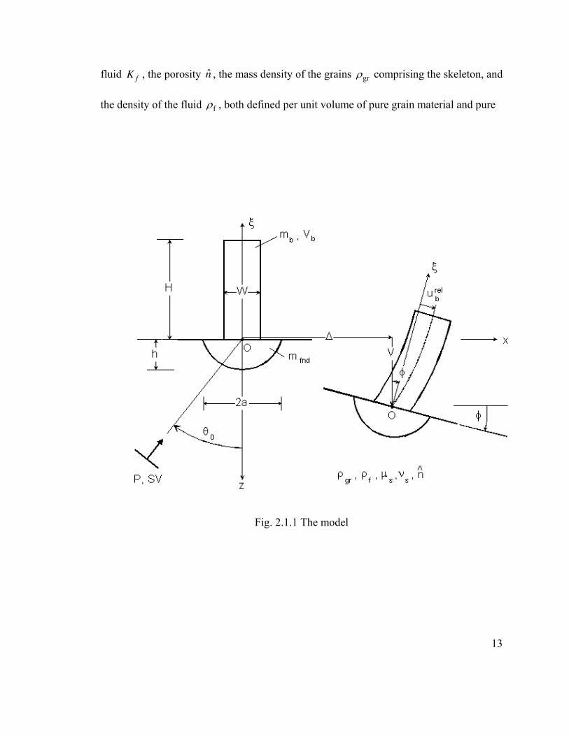
fluid fK , the porosity , the mass density of the grains n̂ grρ comprising the skeleton, and

the density of the fluid fρ , both defined per unit volume of pure grain material and pure

Fig. 2.1.1 The model

13

fluid. This implies shear wave velocity of the dry mixture ,dry grˆ/[(1 ) ]S sV nµ ρ= − . The

skeleton and the foundation are perfectly bonded to each other. The motion of the fluid

along the contact surface relative to that of the solid is constrained by the drainage

condition. It is assumed in this thesis work that the foundation can be either completely

permeable, allowing for free drainage of the pore fluid, or completely impermeable.

These conditions would affect the foundation complex stiffness matrix, and the

foundation driving forces. The half-space surface can also be either perfectly sealed or

unsealed, and this would affect the free-field motion (Lin et al., 2001, 2005).

A closed form solution is obtained by: (1) expanding the scattered waves (a

perturbation to the free-field motion caused by the presence of the foundation) in a series

of outgoing cylindrical waves (represented by Hankel functions in space), (2) expressing

the coefficients of this expansion in terms of the (known) coefficients of expansion of the

free-field motion and the (unknown) motion of the rigid foundation through the

continuity of displacements at the contact surface, and (3) solving for the motion of the

foundation from the dynamic equilibrium conditions. In this process, the zero-stress

condition on the half-space surface, which is automatically satisfied by the free-field

motion, is relaxed for the scattered waves, as in Todorovska and Al Rjoub (2006a). The

zero stress condition for the scattered waves can be imposed numerically along finite

length of the half-space surface adjacent to the foundation, by some point collocation or a

weighted residual method, for example. In the interest of simplicity, and in view of all

the other simplifications in this model (e.g., the restriction of the shape of the foundation,

the assumption that it is absolutely rigid, the assumption of perfect bond at the contact

14

15

5

surface, and finally – the assumption of liner constitutive relations and small

displacements, and of homogeneous and isotropic soil), it was decided to relax this

condition. De Barros and Luco (1995) compared foundation impedances for a semi-

circular foundation in an elastic half-space, when the zero-stress boundary condition is

imposed on the scattered waves, and when it is relaxed. Their results show that for

horizontal and vertical motions the difference is small (the approximate solution

overestimates slightly the damping and the vertical stiffness, while it underestimated

slightly the horizontal stiffness at smaller frequencies and overestimates it slightly for

higher frequencies). The difference is also small for the coupling terms (between

horizontal motion and rocking). The difference is the largest for the rocking motions at

low frequencies, especially for the damping coefficient. The approximate solution

overestimates the rocking stiffness and underestimates the damping at all frequencies in

the range 0 / Sa a Vω= < , but the difference becomes progressively smaller as the

frequency increases. At 0 0.5a = , the rocking stiffness is overestimated by as much as

about 28%, and the damping coefficient is underestimated by as much as 38%, but the

shapes of the functions are similar, and the difference rapidly decreases with frequency,

especially for the damping coefficient. However, it turns out that the rocking stiffness is

not noticeably affected by the fluid in the pores, as shown in the companion paper, and

therefore the conclusions of this study are not likely to be affected by this approximation.

2.2 Wave Propagation in Fluid Saturated Poroelastic Medium

The motion in the soil is assumed to be governed by Biot’s theory of wave

propagation in a fully saturated poroelastic medium (1956a), which was postulated based

on the assumption that the motion of the solid matrix is a wave motion, while that of the

fluid relative to the solid is a diffusion process described by Darcy’s law. Biot (1956a)

made the following assumptions:

1. The Reynolds number is less than 2000, which implies that the relative motion of

the fluid in the pores is laminar flow.

2. The size of the unit element of the solid-fluid mixture is much smaller than the

wavelength of the motions considered.

3. The size of the unit element of the mixture is large compared to the size of the

pores.

Then the motion of the solid and that of the fluid is described by the following two

coupled equations of motion

( ) ( ) ( )

[ ] ( ) ( )

22

11 122

2

11 122

ˆgrad

ˆgrad

u e Q u U bt

Qe R u U b u Ut t

µ λ µ ε ρ ρ

ε ρ ρ

∂ ∂⎡ ⎤∇ + + + = + + −⎣ ⎦ ∂ ∂

∂ ∂+ = + − −

∂ ∂

u Ut

(2.2.1)

where

u = displacement vector for the solid-skeleton

U = displacement vector for the pore fluid

( )e div u=

16

( )div Uε =

11 12 22, ,ρ ρ ρ = dynamic mass coefficients

b̂ = coefficient of dissipation

The coefficient of dissipation depends on the permeability of the skeleton and on

the viscosity of the fluid via the relation

b̂

2 ˆˆ ˆˆ

b nk

µ=

where

n̂ = porosity

µ̂ = absolute viscosity in units Pa s=kg/(m s)⋅ ⋅

k̂ = intrinsic permeability (depends only on the properties of the skeleton) in units 2m

Hence, ˆ /b ω has units of mass density.

Helmholtz decomposition to the displacement vector gives

( ) ( )grad curlu φ ψ= + (2.2.2a)

( ) ( )grad curlU = Φ + Ψ (2.2.2b)

where φ and are the P-wave potentials, and Φ ψ and Ψ are the S-wave potentials for the

solid and fluid, respectively. Substitution of eqns (2.2.2a,b) into eqn (2.2.1) leads to the

following two sets of equations for the P-wave and S-wave potentials

17

( ) ( )

( ) ( )

22 2

11 122

22 2

11 122

ˆ

ˆ

P Q bt

Q R bt t

φ ρ φ ρ

φ ρ φ ρ

∂ ∂∇ + ∇ Φ = + Φ + −Φ

∂ ∂∂ ∂

∇ + ∇ Φ = + Φ − −Φ∂ ∂

tφ

φ (2.2.3)

and

( ) ( )

( ) ( )

22

11 122

2

11 122

ˆ

ˆ0

bt

bt t

µ ψ ρ ψ ρ ψ

ρ ψ ρ ψ

∂ ∂∇ = + Ψ + −Ψ

∂ ∂∂ ∂

= + Ψ − −Ψ∂ ∂

t (2.2.4)

2.3 Solution for P-waves

For harmonic wave motion, the potentials can be represented as

( )

1

i kx tc e

ωφ += , (

2

i kx tc e

)ω+Φ = (2.2.5)

( )

3

i kx tc e

ωψ += , (

4

i kx tc e

)ω+Ψ = (2.2.6)

Substitution of eqn (2.2.5) into eqn (2.2.3) leads to the following fourth order differential

equation for the P-wave potential in the solid

4 2 0A B Cφ φ− + = (2.2.7a)

where

2A PR Q= − (2.2.7b)

11 22 122 (ib

2 )B R P Q P R Qρ ρ ρω

= + − − + + (2.2.7c)

2

11 22 12 11 22 12( 2ib

C )ρ ρ ρ ρ ρ ρω

= − − + + (2.2.7d)

Further, eqn (2.2.7) can be decomposed into the following two equations

( )2 2

, 0j jkα φ∇ + = , j=1,2 (2.2.8)

18

where

,

,

j

j

kV

αα

ω= , j=1,2 (2.2.9a)

and

( ), 1

2 2

2

4j

AV

B B ACα =

−∓ , j=1,2 (2.2.9b)

are the wave numbers and wave velocities of two distinct P-waves (fast and slow) in the

solid.

The wave potential for the fluid can be obtained after substituting eqn (2.2.5) into

eqn (2.2.3), which gives

1 2 1 1 2 2f fφ φΦ = Φ +Φ = + (2.2.10)

where

2

, 11 12

12 22

( / )( )

( / )( )

j

j

A V R Q ib Q Rf

R Q ib Q R

α ρ ρ ωρ ρ ω− + + +

=− + +

, j=1,2 (2.2.11)

2.3.1 Solutions for S-waves

Substitutin of eqn (2.2.6) into eqn (2.2.2) leads to the following differential equation

for the S-wave potential of the motion of the skeleton

( )2 2 0kβ ψ∇ + = (2.2.12)

where

kV

ββ

ω= (2.2.13a)

19

and

22

2

11 22 12 11 22 12

( / )

( 2 )*

ibV

ibβ

µ ρ ω/ρ ρ ρ ρ ρ ρ ω

−=

− − + + (2.2.13b)

are the wave number and wave velocity of the shear waves in the skeleton.

The wave potential for the fluid can be obtained as

3fψΨ = (2.2.14)

where

123

22

( /

( /

ibf

ib

)

)

ρ ωρ ω

+= −

− (2.2.15)

2.3.2 Material Constants for the Mixture

The material constants of mixtures can be determined experimentally (Biot and

Willis, 1957), or can be derived from the properties of the components. In the

dimensionless analysis in this work, the set of input parameters consists of the porosity

, the Poisson’s ratio of the skeleton n̂ sν , the ratio of the bulk modulus of the fluid and

the shear modulus of the skeleton /fK sµ , and the ratio of the mass density of the fluid

and that of the grains /f grρ ρ (both per unit volume of “pure” material).

The elastic moduli of the mixture µ , λ , R and are computed using a

simplification (for

Q

R and ) of the formulae proposed by Biot and Willis (1957) based

on the assumption that the compressibility of the mixture is much smaller than that of the

solid skeleton and of the fluid, and can be neglected, which is a common assumption in

soil mechanics (Lin et al., 2005)

Q

20

( )

2 /

ˆ1

ˆ

s

s

f

f

Q R

Q n K

R nK

µ µ

λ λ

=

= +

= −

=

(2.2.16)

where

2

1 2

ss s

s

v

vλ µ=

−= Lamé constant for the skeleton

For computation of the mass coefficients, 11ρ , 22ρ and 12ρ , the following relations

proposed by Berryman (1980) are used (as in Lin et al., 2005)

( )

( )

11 gr 12

22 f 12

12 f

ˆ1

ˆ

ˆ 1

n

n

n α

ρ ρ ρ

ρ ρ ρρ τ ρ

= − −

= −

= − −

(2.2.17)

where

ˆ11

ˆr

n

nατ τ −= + ≥1= dynamic tortuosity (2.2.18a)

Tortuosity is a dimensionless macroscopic parameter characterizing the resistance to

flow of a fluid in porous medium, in particular the effect that, on microscopic scale, the

paths of the fluid particles deviate from a straight line. It depends on the porosity, , as

well as on the shape of the pores, through the parameter

n̂

rτ . It has values 1 ατ≤ < ∞ . As

(pure fluid) ˆ 1n → 1ατ → , and as (pure solid) ˆ 0n → ατ →∞ . For pores formed by

spherical grains, as assumed in this work, 1/ 2rτ = , and

21

1 11

ˆ2 nατ

⎛= +⎜⎝ ⎠

⎞⎟ (2.2.18b)

It can be seen from eqn (2.2.17) that the dynamic mass coefficients represent physically

mass densities, per unit volume of the mixture. If the coupling term 12ρ is neglected,

then 11ρ and 22ρ represent the mass densities of the solid and fluid phases per unit

volume of the mixture.

2.3.3 Approximate Treatment of Partial Saturation

Partially saturated soil represents a three-phase medium (mixture of solid, fluid and

gas). So far there is no generally accepted theory for wave propagation in such soil

medium. In this work, a simplified approach is followed, in which is the theory for a

two-phase medium is used, but with reduced bulk modulus of the fluid, as in Yang

(2001). Let be the degree of saturation. The relative proportions of the constituent

volumes are defined as

rS

/V tn V V= (2.2.19a)

/r WS V V= V (2.2.19b)

where n is the porosity of the soil, and and are respectively the volumes of

pores, pore water and the total volume.

,V WV V tV

In this study, a high degree of saturation is considered > 90%, assuming the

embedded air in the pore water is in the form of bubbles uniformly distributed through

the fluid. In this case, the bulk modulus of fluid fK can be written as

22

1

11fr

W a

KS

K P

=−

+ (2.2.20)

Where is the bulk modulus of pore water and is the absolute fluid pressure. WK aP

23

2.4 The Soil-Structure Interaction Problem

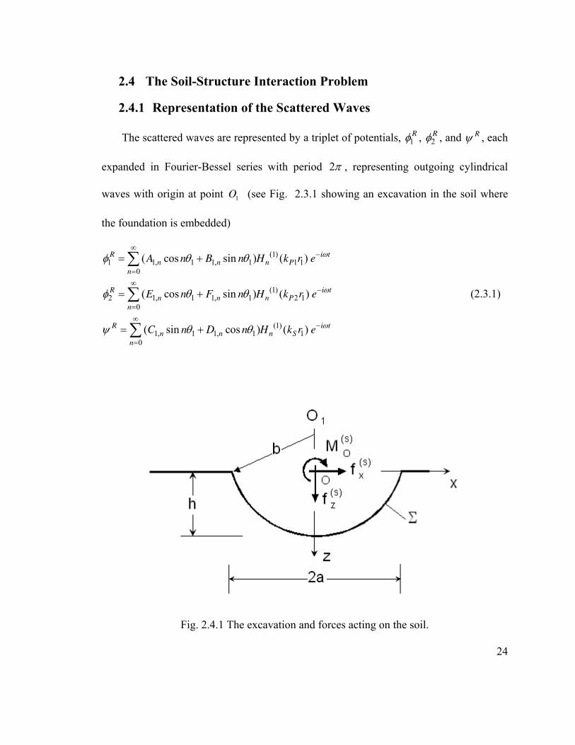
2.4.1 Representation of the Scattered Waves

The scattered waves are represented by a triplet of potentials, 1Rφ , 2

Rφ , and Rψ , each

expanded in Fourier-Bessel series with period 2π , representing outgoing cylindrical

waves with origin at point (see Fig. 2.3.1 showing an excavation in the soil where

the foundation is embedded)

1O

(1)1 1, 1 1, 1 1 1

0

(1)2 1, 1 1, 1 2 1

0

(1)1, 1 1, 1 1

0

( cos sin ) ( )

( cos sin ) ( )

( sin cos ) ( )

R i tn n n P

n

R i tn n n P

n

R i tn n n S

n

A n B n H k r e

E n F n H k r e

C n D n H k r e

ω

ω

ω

φ θ θ

φ θ θ

ψ θ θ

∞−

=∞

−

=∞

−

=

= +

= +

= +

∑

∑

∑

(2.3.1)

Fig. 2.4.1 The excavation and forces acting on the soil.

24

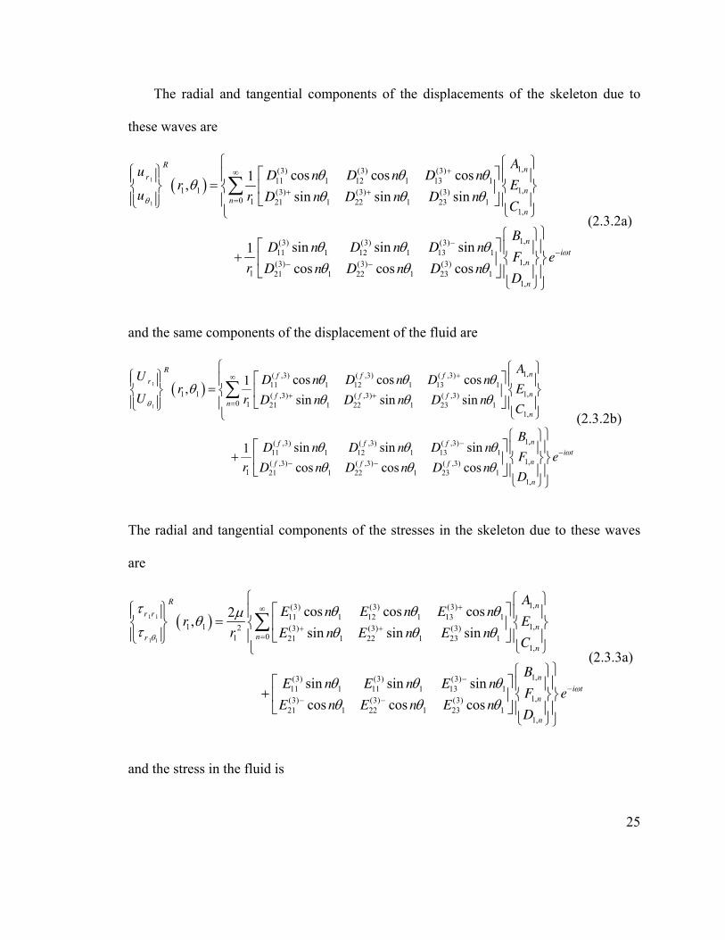
The radial and tangential components of the displacements of the skeleton due to

these waves are

( )1

1

1,(3) (3) (3)

11 1 12 1 13 1

1 1 1,(3) (3) (3)0 1 21 1 22 1 23 1

1,

(3) (3) (3)

11 1 12 1 13 1

(3)

1 21 1 2

cos cos cos1,

sin sin sin

sin sin sin1

cos

Rn

r

n

n

n

Au D n D n D n

r Eu r D n D n D n

C

D n D n D n

r D n D

θ

θ θ θθ

θ θ θ

θ θ θθ

+∞

+ +=

−

−

⎧ ⎧ ⎫⎧ ⎫ ⎡ ⎤⎪⎪ ⎪ ⎪ ⎪=⎨ ⎬ ⎨ ⎨ ⎬⎢ ⎥⎪ ⎪ ⎣ ⎦⎪ ⎪⎩ ⎭

⎩ ⎭⎩

+

∑

1,

1,(3) (3)

2 1 23 1

1,

cos cos

n

i t

n

n

B

F en D n

D

⎪

ω

θ θ−

−

⎫⎧ ⎫⎡ ⎤ ⎪⎪ ⎪

⎨ ⎬⎬⎢ ⎥⎣ ⎦ ⎪ ⎪⎪

⎩ ⎭⎭

(2.3.2a)

and the same components of the displacement of the fluid are

( )1

1

1,( ,3) ( ,3) ( ,3)

11 1 12 1 13 1

1 1 1,( ,3) ( ,3) ( ,3)0 1 21 1 22 1 23 1

1,

( ,3) ( ,3) ( ,3)

11 1 12 1 13

1

cos cos cos1,

sin sin sin

sin sin sin1

Rnf f f

r

nf f fn

n

f f f

AU D n D n D n

r EU r D n D n D n

C

D n D n D

r

θ

θ θ θθ

θ θ θ

θ θ

+∞

+ +=

−

⎧ ⎧ ⎫⎧ ⎫ ⎡ ⎤⎪⎪ ⎪ ⎪ ⎪=⎨ ⎬ ⎨ ⎨ ⎬⎢ ⎥⎪ ⎪ ⎣ ⎦⎪ ⎪⎩ ⎭

⎩ ⎭⎩

+

∑

1,

1

1,( ,3) ( ,3) ( ,3)

21 1 22 1 23 1

1,

cos cos cos

n

i t

nf f f

n

Bn

F eD n D n D n

D

⎪

ωθθ θ θ

−− −

⎫⎧ ⎫⎡ ⎤ ⎪⎪ ⎪

⎨ ⎬⎬⎢ ⎥⎣ ⎦ ⎪ ⎪⎪

⎩ ⎭⎭

(2.3.2b)

The radial and tangential components of the stresses in the skeleton due to these waves

are

( )1 1

1 1

1,(3) (3) (3)

11 1 12 1 13 1

1 1 1,2 (3) (3) (3)01 21 1 22 1 23 1

1,

(3) (3)

11 1 11

cos cos cos2,

sin sin sin

sin

Rn

r r

n

nr

n

AE n E n E n

r Er E n E n E n

C

E n E

θ

τ θ θ θµθτ θ θ θ

θ

+∞

+ +=

⎧ ⎧ ⎫⎧ ⎫ ⎡ ⎤⎪⎪ ⎪ ⎪ ⎪=⎨ ⎬ ⎨ ⎨ ⎬⎢ ⎥⎪ ⎪ ⎣ ⎦⎪ ⎪⎩ ⎭

⎩ ⎭⎩

+

∑

1,(3)

1 13 1

1,(3) (3) (3)

21 1 22 1 23 1

1,

sin sin

cos cos cos

n

i t

n

n

Bn E n

F eE n E n E n

D

⎪

ωθ θθ θ θ

−−

− −

⎫⎧ ⎫⎡ ⎤ ⎪⎪ ⎪

⎨ ⎬⎬⎢ ⎥⎣ ⎦ ⎪ ⎪⎪

⎩ ⎭⎭

(2.3.3a)

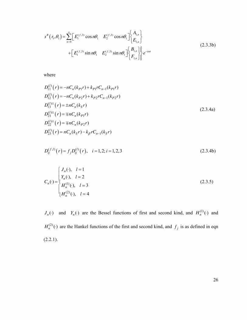
and the stress in the fluid is

25

( ) 1,( ,3) ( ,3)

1 1 1 1 2 1

0 1,

1,( ,3) ( ,3)

1 1 2 1

1,

, cos cos

sin sin

nR f f

n n

nf f i

n

As r E n E n

E

Bt

E n E n eF

ω

θ θ θ

θ θ

∞

=

−

⎧ ⎫⎡ ⎤= ⎨ ⎬⎣ ⎦

⎩ ⎭⎫⎧ ⎫⎪⎡ ⎤+ ⎨ ⎬⎬⎣ ⎦ ⎪⎩ ⎭⎭

∑ (2.3.3b)

where

( )( )( )( )( )( )

( )1 1 1 111

( )2 2 1 212

( )13

( )121

( )222

( )123

( ) ( )

( ) ( )

( )

( )

( )

( ) ( )

ln P P n P

ln P P n P

ln S

ln P

ln P

ln S n S

D r nC k r k rC k r

D r nC k r k rC k r

D r nC k r

D r nC k r

D r nC k r

D r nC k r k rC k rβ

−

−

±

±

±

−

= − +

= − +

= ±

=

=

= −

∓

∓

(2.3.4a)

( ) ( )( , ) ( ) , 1, 2; 1,2,3f l lij j ijD r f D r i i= = = (2.3.4b)

(1)

(2)

( ), 1

( ), 2( )

( ), 3

( ), 4

n

n

nn

n

J l

Y lC

H l

H l

⋅ =⎧⎪ ⋅ =⎪⋅ = ⎨ ⋅ =⎪⎪ ⋅ =⎩

(2.3.5)

( )nJ ⋅ and are the Bessel functions of first and second kind, and ( )nY ⋅ (1) ( )nH ⋅ and

are the Hankel functions of the first and second kind, and (2) ( )nH ⋅ jf is as defined in eqn

(2.2.1).

26

( )

( )

( )

( ) 2 2 21 1 1 1 111

( ) 2 2 22 2 2 2 2 112

( )113

1 1( ) ( ) ( ) 1 ( ) ( )

2 2 2

1 1( ) ( ) ( ) 1 ( ) (

2 2 2

( 1) ( ) ( )

lP n P f n f P n P

lP n P P n P P n P

ln S S n

E r n n k r C k r k r Q C k r k rC k r

E r n n k r C k r k r Q C k r k rC k r

E r n n C k r k rC k rβ

λ

λ

−

−

±−

⎡ ⎤ ⎛ ⎞= + − − + + −⎜ ⎟⎢ ⎥⎣ ⎦ ⎝ ⎠⎡ ⎤ ⎛ ⎞= + − − + + −⎜ ⎟⎢ ⎥⎣ ⎦ ⎝ ⎠

⎡ ⎤= − + +⎣∓

( ) [ ]( ) [ ]

( )

2 )

( )1 1 1 121

( )2 2 1 222

( ) 2 2123

( 1) ( ) ( )

( 1) ( ) ( )

1( ) ( ) ( )

2

ln P P n P

ln P P n P

lS n S S n S

E r n n C k r k rC k r

E r n n C k r k rC k r

E r n n k r C k r k rC k r

±−

±−

−

⎦

= − + +

= − + +

⎡ ⎤= − + − −⎢ ⎥⎣ ⎦

∓

∓

(2.3.6a)

( )

( )

( )

( , ) 2

11 1 1 1

( , ) 2

12 2 2 2

( , )

13

1( ) ( )

2

1( ) (

2

0

f l

P n P

f l

P n P

f l

E r S k r C k r

E r S k r C k r

E r

=

=

=

) (2.3.6b)

where

( ) / , 1, 2j jS Q f R jµ= + = (2.3.7)

2.4.2 Boundary Conditions at the Contact Surface

The motion of the rigid foundation for incident monochromatic waves is harmonic,

and can be written as

0

0

0

e i t

V V

a a

ω

ϕ ϕ

−

⎧ ⎫ ⎧ ⎫⎪ ⎪ ⎪ ⎪∆ = ∆⎨ ⎬ ⎨ ⎬⎪ ⎪ ⎪ ⎪⎩ ⎭ ⎩ ⎭

(2.3.8)

Along the contact surface 1 0 0: ,r b θ θ θΣ = − ≤ ≤ 10 sin ( / )a bθ −=, (Fig. 2.3.1), the

displacements of the skeleton are constrained by the displacements of the foundation, and

the motion of the fluid is constrained by the drainage condition. Perfect bond between

27

the skeleton and the foundation, and perfectly sealed contact (i.e. no drainage of the pore

fluid) imply

( ) ( )

1 1

1 1

1 1 1 1

1 1 1 0

1 1 1 0

0

cos sin ( / )sin

sin cos / ( / ) cos e

0 0 0

ff R

r r

i t

r r r r

u u d a V

u u b a d a

au U u U

ωθ θ

θ θ θθ θ θ

ϕ

−

Σ Σ

⎧ ⎫ ⎧ ⎫⎡ ⎤⎪ ⎪ ⎪ ⎪⎪ ⎪ ⎪ ⎪ ⎪ ⎪⎢ ⎥+ = − − + ∆⎨ ⎬ ⎨ ⎬ ⎨ ⎬⎢ ⎥

⎪ ⎪ ⎪ ⎪ ⎪ ⎪⎢ ⎥⎣ ⎦− −⎪ ⎪ ⎪ ⎪⎩ ⎭ ⎩ ⎭

⎧ ⎫

⎩ ⎭

(2.3.9a)

Where the matrix on the right-hand side is the foundation influence matrix.

Similarly, perfect bond between the skeleton and the foundation, and unsealed contact

(i.e. free drainage of the pore fluid) imply

1 1

1 1

1 1 1 0

1 1 1 0

0

cos sin ( / )sin

sin cos / ( / ) cos e

0 0 0

ff R

r r

i t

u u d a V

u u b a d a

as s

ωθ θ

θ θ θθ θ θ

ϕ

−

Σ Σ

⎧ ⎫ ⎧ ⎫ ⎡ ⎤⎪ ⎪ ⎪ ⎪ ⎪ ⎪⎢ ⎥+ = − − + ∆⎨ ⎬ ⎨ ⎬ ⎨ ⎬⎢ ⎥⎪ ⎪ ⎪ ⎪ ⎪ ⎪⎢ ⎥⎣ ⎦⎩ ⎭ ⎩ ⎭

⎧ ⎫

⎩ ⎭

(2.3.9b)

The application of these conditions enables expressing the unknown coefficients of

expansion of the scattered waves in terms of the known free-field displacements, and the

displacements of the foundation. However, this requires expansion of the free-field

displacements at in Fourier series of 1r b= 1θ with period 2π . This can be done by

expanding the potentials in Fourier-Bessel series, and then computing the displacements,

similarly as for the scattered waves, but such series converge only for the plane waves,

and diverge for the surface waves (Lee and Cao, 1989). Hence, for the surface waves, we

expand the displacements at 1r b= in Finite Fourier series of 1θ , up to , which is

the truncation index for the expansion of the scattered and plane free-field waves (Lee

n N=

28

and Cao, 1989). Let us assume that such expansions are available, with nAi and

being the Fourier coefficients for the symmetric and anti-symmetric terms. Then

nBi

( ) ( ) ( )

1

1

1 1

1 1

1

0

1 1

cos sin1

sin cos

cos sin

r r

r r r r

ff

u ur n nN

u u

n n

nu U u U

n n n nr r

u A n B n

u A n Bb

A A n B B nu U

θ θθ

θ θθ

θ θ=

Σ

⎧ ⎫ ⎧ ⎫⎧ ⎫ ⎧⎪ ⎪ ⎪ ⎪⎪ ⎪ ⎪⎪ ⎪ ⎪⎪ ⎪ ⎪ ⎪⎪= +⎨ ⎬ ⎨⎨ ⎬ ⎨ ⎬⎬⎪ ⎪ ⎪⎪ ⎪ ⎪ ⎪⎪− −− ⎪ ⎪ ⎪⎪ ⎪ ⎪⎩ ⎭ ⎩⎩ ⎭⎩ ⎭

∑ 1nθ

⎫⎪

⎪⎪⎭

(2.3.10a)

and

1

1

1 1

1

0

1 1

cos sin1

sin cos

cos sin

r r

ffu u

r n nNu u

n n

n s s

n n

u A n B n

u A n Bb

A n B ns

θ θθ

θ θθθ θ=

Σ

⎧ ⎫⎧ ⎫ ⎧ ⎫ ⎧⎪ ⎪⎪ ⎪ ⎪ ⎪ ⎪= +⎨ ⎬ ⎨⎨ ⎬ ⎨ ⎬⎬

⎪ ⎪ ⎪⎪ ⎪ ⎪ ⎪⎪⎩ ⎭ ⎩⎩ ⎭ ⎩ ⎭

∑ 1nθ⎫⎪

⎭

(2.3.10b)

For the scattered waves

( )

1

1

1 1

(3) (3) (3)

11 1 12 1 13 1 1,

(3) (3) (3)

21 1 22 1 23 1 1,

0 ( ,3) ( ,3) ( ,3)

11 1 12 1 13 1 1,

cos cos cos1

sin sin sin

cos cos cos

R

r nN

n

n rel rel rel

nr r

u D n D n D n A

u D n D n D n Eb

D n D n D n Cu U

θ

θ θ θθ θ θθ θ θ=

ΣΣ

⎧ ⎫ ⎧⎡ ⎤ ⎧ ⎫⎪ ⎪ ⎪⎢ ⎥⎪ ⎪ ⎪=⎨ ⎬ ⎨ ⎨⎢ ⎥⎪ ⎪ ⎪ ⎪⎢ ⎥ ⎩ ⎭⎣ ⎦− ⎩⎪ ⎪⎩ ⎭

∑

(3) (3) (3)

11 1 12 1 13 1 1,

(3) (3) (3)

21 1 22 1 23 1 1,

( ,3) ( ,3) ( ,3)

11 1 12 1 13 1 1,

cos cos cos

sin sin sin

cos cos cos

n

n

rel rel rel

n

D n D n D n B

D n D n D n F

D n D n D n D

θ θ θθ θ θθ θ θ

Σ

⎫⎡ ⎤ ⎧ ⎫⎪⎢ ⎥ ⎪ ⎪+ ⎨ ⎬⎢ ⎥

⎪ ⎪⎢ ⎥ ⎩ ⎭⎣ ⎦ ⎭

⎪⎬⎪

⎬⎪

(2.3.11a)

where

( ,3) ( ,3) (3)rel f

ij ij ijD D D= − (2.3.11b)

and

29

1

1

(3) (3) (3)

11 1 12 1 13 1 1,

(3) (3) (3)

21 1 22 1 23 1 1,

0 ( ,3) ( ,3) ( ,3)

11 1 12 1 13 1 1,

(3)

11

cos cos cos1

sin sin sin

cos cos cos

c

R

r nN

n

n f f f

n

u D D D A

u D D Db

E E E Cs

D

θ

θ θ θθ θ θθ θ θ=

ΣΣ

⎧⎧ ⎫ ⎡ ⎤

E

⎧ ⎫⎪⎪ ⎪ ⎢ ⎥ ⎪ ⎪=⎨ ⎬ ⎨ ⎨ ⎬⎢ ⎥

⎪ ⎪ ⎪ ⎪ ⎪⎢ ⎥ ⎩ ⎭⎣ ⎦⎩ ⎭ ⎩

+

∑

(3) (3)

1 12 1 13 1 1,

(3) (3) (3)

21 1 22 1 23 1 1,

( ,3) ( ,3) ( ,3)

11 1 12 1 13 1 1,

os cos cos

sin sin sin

cos cos cos

n

n

f f f

n

D D B

D D D F

E E E D

θ θ θθ θ θθ θ θ

Σ

⎫⎡ ⎤ ⎧ ⎫⎪⎢ ⎥ ⎪ ⎪

⎨ ⎬⎬⎢ ⎥⎪ ⎪⎪⎢ ⎥ ⎩ ⎭⎣ ⎦ ⎭

(2.3.11c)

After substitution for the appropriate expansions in eqn’s (2.3.11a) and (2.3.11b),

and matching the terms multiplying the same basis functions (due to the orthogonality of

Fourier series), the coefficients of expansion of the scattered field can be expressed in

terms of the coefficients of expansion of the free-field motion and the displacements of

the foundation. Then for sealed boundary

1, 01

(3)

1, ,sealed 0

01,

1, 01

(3)

1, ,sealed

1,

( ) , 0,...,

( )

r

r r

r

r r

un n

u

n n

u U

n nn

un n

u

n n

u U

n nn

A A V

E D A X n n

A A aC

B B V

F D B X n

B BD

θ

θ

ϕ

−+ +Σ

−− −Σ

⎧ ⎫⎧ ⎫ ⎧ ⎫ ⎧ ⎫⎪ ⎪⎪ ⎪ ⎪ ⎪ ⎪ ⎪⎡ ⎤ ⎡ ⎤= − + ∆ =⎨ ⎬ ⎨ ⎨ ⎬ ⎨ ⎬⎬⎣ ⎦ ⎣ ⎦

⎪ ⎪ ⎪ ⎪ ⎪ ⎪ ⎪⎪− ⎩ ⎭⎩ ⎭⎩ ⎭ ⎩⎧ ⎫ ⎧ ⎫⎪ ⎪ ⎪ ⎪⎡ ⎤ ⎡ ⎤= − + ∆⎨ ⎬ ⎨ ⎬⎣ ⎦ ⎣ ⎦⎪ ⎪ ⎪ ⎪−⎩ ⎭⎩ ⎭

0

0

, 0,...,n N

aϕ

⎧ ⎫⎧ ⎫⎪ ⎪⎪ ⎪ =⎨ ⎨ ⎬⎬⎪ ⎪ ⎪⎪

⎩ ⎭⎩ ⎭

N

⎭

N

(2.3.12a)

and for an unsealed boundary

1, 01

(3)

1, ,unsealed 0

01,

1, 01

(3)

1, ,unsealed 0

01,

( ) , 0,...,

( )

r

r

un n

u

n n

s

nn

un n

u

n n

s

nn

A A V

E D A X n n

A aC

B B V

F D B X n

B aD

θ

θ

ϕ

ϕ

−+ +Σ

−+ −Σ

⎧ ⎫⎧ ⎫ ⎧ ⎫ ⎧ ⎫⎪ ⎪⎪ ⎪ ⎪ ⎪ ⎪ ⎪⎡ ⎤ ⎡ ⎤= − + ∆ =⎨ ⎬ ⎨ ⎨ ⎬ ⎨ ⎬⎬⎣ ⎦ ⎣ ⎦

⎪ ⎪ ⎪ ⎪ ⎪ ⎪ ⎪⎪⎩ ⎭⎩ ⎭⎩ ⎭ ⎩ ⎭

⎧ ⎫ ⎧ ⎫ ⎧⎪ ⎪ ⎪ ⎪ ⎪⎡ ⎤ ⎡ ⎤= − + ∆⎨ ⎬ ⎨ ⎬ ⎨⎣ ⎦ ⎣ ⎦⎪ ⎪ ⎪ ⎪

⎩⎩ ⎭⎩ ⎭

, 0,...,n N

⎧ ⎫⎫⎪ ⎪⎪ =⎨ ⎬⎬⎪ ⎪ ⎪⎪

⎭⎩ ⎭

(2.3.12b)

30

where

31

n b

⎦

=

=

( )

( )

(3) (3) (3)

11 12 13

(3) (3) (3) (3)

,sealed 21 22 23

( ,3) ( ,3) ( ,3)

11 12 13

(3) (3) (3)

11 12 13

(3) (3) (3) (3)

,unsealed 21 22 23

( ,3) ( ,3) ( ,3)

11 12 13

,

,

rel rel rel

f f f

D D D

D D D D

D D D

D D D

D D D D n b

E E E

±

±Σ

±

±Σ

⎡ ⎤⎢ ⎥⎡ ⎤ = ⎢ ⎥⎣ ⎦⎢ ⎥⎣

⎡ ⎤⎢ ⎥⎡ ⎤ = ⎢ ⎥⎣ ⎦⎢ ⎥⎣ ⎦

(2.3.13)

1 0 0

( ) 0 0 0 , 1

0 0 0

0 0 0

( ) 0 0 0 , 1

0 0 0

X n n

X n n

+

+

−⎡ ⎤⎢ ⎥⎡ ⎤ = =⎣ ⎦ ⎢ ⎥⎢ ⎥⎣ ⎦⎡ ⎤⎢ ⎥⎡ ⎤ = ≠⎣ ⎦ ⎢ ⎥⎢ ⎥⎣ ⎦

(2.3.14a)

0 0 0

( ) 0 0 / , 0

0 0 0

0 1 /

( ) 0 1 / , 1

0 0 0

0 0 0

( ) 0 0 0 , 1

0 0 0

X n b a n

d a

X n d a n

X n n

−

−

−

⎡ ⎤⎢ ⎥⎡ ⎤ = −⎣ ⎦ ⎢ ⎥⎢ ⎥⎣ ⎦⎡ ⎤⎢ ⎥⎡ ⎤ =⎣ ⎦ ⎢ ⎥⎢ ⎥⎣ ⎦⎡ ⎤⎢ ⎥⎡ ⎤ = >⎣ ⎦ ⎢ ⎥⎢ ⎥⎣ ⎦

(2.3.14b)

2.4.3 Integral of Stresses along the Contact Surface

Next we compute vertical and horizontal forces ( )s

zf and ( )s

xf , and moment about O ,

( )

0

sM , which result from all stresses in the soil along the contact surface , and have

signs as shown in Fig. 2.3.1. We also introduce a generalized force vector notation for

Σ

this triplet of forces and moment { }0, , /T

z xf f M a=F and refer to it as the force, and

generalized displacement vector { }, ,T

V aϕ= ∆∆ and refer to it as the displacement. For

harmonic excitation, is also harmonic and can be written as ∆

0i t

eω−=∆ ∆ (2.3.15)

where is its complex amplitude. 0∆

The resultant force vector, ( )sF , is the sum of the force vectors due to the free-field

motion and due to the scattered waves, ( )s

ffF and ( )s

RF , and can be computed as follows

0

1 1 1 1

1 1 1 10

( ) ( ) ( )

1 1

1 1

1 1

cos sin

sin cos

( / )sin / ( / ) cos

s s s

ff R

ff R

r r r r

r r

s sb d

d a b a d a

θ

θ θθ

θ θ τ τ1θ θ θ

τ τθ θ− Σ Σ

= +

− +⎡ ⎤ ⎧ ⎫+ +⎧ ⎫ ⎧ ⎫⎪⎪ ⎪ ⎪ ⎪ ⎪⎢ ⎥= − − +⎨⎨ ⎬ ⎨ ⎬ ⎬⎢ ⎥ ⎪ ⎪ ⎪ ⎪⎪ ⎪⎩ ⎭ ⎩ ⎭⎢ ⎥ ⎩ ⎭− −⎣ ⎦∫

F F F

(2.3.16)

Eqn (2.36) holds for both sealed and unsealed conditions. We note however that, for

an unsealed boundary, the total stress in the pore fluid, ff

s sR+ , is actually zero on the

boundary, as preset by the drainage condition (see eqn (2.29b)).

Similarly as in Section 2.3.1, we expand the stresses of the free-field motion along

the contact surface in Fourier series of 1θ with period 2π

1 1

1 1

1

20 1 1

( ) cos ( )sin2

sin cos

rr rr

r r

ffs sN

r r n n n n i t

nr n n

s A A n B B ne

b A n B nθ θ

τ τ1 ω

τ τθ

τ θ θµτ θ θ

−

=Σ

⎧ ⎫+⎧ ⎫ ⎧ ⎫ ⎧+ +⎪ ⎪ ⎪⎪ ⎪ ⎪ ⎪⎪= +⎨ ⎬ ⎨⎨ ⎬ ⎨ ⎬⎬⎪ ⎪ ⎪⎪ ⎪ ⎪ ⎪⎩ ⎭ ⎩⎩ ⎭ ⎩ ⎭

∑⎫

⎪⎭

(2.3.17)

and substitute in eqn (2.3.16). Then, for the forces due to the free-field motion we get

32

( )

0

2( ) ( )

rr rr

r r

s sNn n n ns i t

ff

n n n

A A B BL n L n e

b A Bθ θ

τ τω

τ τ

µ + −

=

⎧ ⎫⎧ ⎫ ⎧ ⎫+ +⎪ ⎪ ⎪ ⎪ ⎪⎪⎡ ⎤ ⎡ ⎤= +⎨ ⎨ ⎬ ⎨ ⎬⎬⎣ ⎦ ⎣ ⎦⎪ ⎪ ⎪ ⎪⎪ ⎪⎩ ⎭ ⎩ ⎭⎩ ⎭

∑F−

1

(2.3.18)

where

[ ]

[ ]

0

0

1 1 1 1

1 1 11

1 1 1 1

1 1 1 1

1 1 1

1 1 1

cos cos sin sin

( ) sin cos cos sin

( / )sin cos / ( / ) cos sin

cos sin sin cos

( ) sin sin cos cos

( / )sin sin / ( / ) cos cos

n

L n n d

d a n b a d a n

n

L n n

d a n b a d a n

θ

θ

θ θ θ θθ θ θ θ

θ θ θ θ

θ θ θ θθ θ θ θ

θ θ θ

+

−

−

⎡ ⎤−⎢ ⎥⎡ ⎤ = − −⎣ ⎦ ⎢ ⎥⎢ ⎥− −⎣ ⎦

−⎡ ⎤ = − −⎣ ⎦

− −

∫

0

0

1

1

d

θ

θ

θ

θθ−

⎡ ⎤⎢ ⎥⎢ ⎥⎢ ⎥⎣ ⎦

∫

(2.3.19)

Some of the terms of matrices ( )L n+⎡ ⎤⎣ ⎦ and ( )L n

−⎡ ⎤⎣ ⎦ are automatically zero (when

the integrand is an odd function), and the nonzero ones can be evaluated analytically,

which gives

1 4

4 1

4 5

( ) ( )

( ) 0 0

0 0

0 0

( ) ( ) ( )

( / ) ( ) ( / ) ( ) ( / ) ( )

I n I n

L n

L n I n I n

d a I n b a I n d a I n

+

−

−⎡ ⎤⎢ ⎥⎡ ⎤ =⎣ ⎦ ⎢ ⎥⎢ ⎥⎣ ⎦⎡ ⎤⎢ ⎥⎡ ⎤ = − −⎣ ⎦ ⎢ ⎥⎢ ⎥− −⎣ ⎦1

(2.3.20)

The expressions for the integrals 1( )I n , 4 ( )I n , and 5( )I n are given in Appendix.

Similarly, for the forces from the scattered waves we get

1, 1,

( ) (3) (3)

1, 1,

0

1, 1,

2( ) ( ) ( ) ( )

n nNs i t

R n

n

n n

A B

L n E n E L n E n F eb

C D

n

ωµ + + − −Σ Σ

=

⎧ ⎫⎧ ⎫ ⎧ ⎫⎪ ⎪⎪ ⎪ ⎪ ⎪⎡ ⎤ ⎡ ⎤ ⎡ ⎤ ⎡ ⎤= +⎨ ⎨ ⎬ ⎨⎣ ⎦ ⎣ ⎦ ⎣ ⎦ ⎣ ⎦⎪ ⎪ ⎪ ⎪

⎩ ⎭ ⎩ ⎭⎩ ⎭

∑F−

⎬⎬⎪⎪

(2.3.21)

33

where

34

)((3) ( ,3) (3) ( ,3) (3) ( ,3)

(3) 11 11 12 12 13 13

(3) (3) (3)

21 22 23

( ) ,f f f

E E E E E EE n n

E E E

±

±Σ

⎡ ⎤+ + +⎡ ⎤ = ⎢ ⎥⎣ ⎦

⎣ ⎦b (2.3.22)

Further, substituting in eqn (2.3.16) for the coefficients of expansion of the scattered

waves from eqn (2.3.12a,b) it follows that for a sealed boundary

01

( ) (3) (3)

R ,sealed 0

0

0

1(3) (3)

,sealed

2( ) ( ) ( )

( ) ( )

r

r r

r

r

u

nNus

n

n u U

n n

u

n

u

n

u

n

A V

L n E n D A b X nb

A A a

B

L n E n D B

B

θ

θ

µ

ϕ

−+ + + +Σ Σ

=

−− − −Σ Σ

⎧ ⎧ ⎫⎧ ⎫ ⎧ ⎫⎪ ⎪ ⎪⎪ ⎪ ⎪ ⎪⎡ ⎤ ⎡ ⎤ ⎡ ⎤ ⎡ ⎤= − +⎨ ⎨ ⎨ ⎬⎣ ⎦ ⎣ ⎦ ⎣ ⎦ ⎣ ⎦⎪ ⎪ ⎪ ⎪− ⎩ ⎭⎩ ⎭⎩ ⎭⎩

⎡ ⎤ ⎡ ⎤ ⎡ ⎤+ −⎣ ⎦ ⎣ ⎦ ⎣ ⎦−

∑F

0

0

0

( )

r

i t

U

n

V

b X n e

B a

∆⎨ ⎬⎬⎪ ⎪⎪

ω

ϕ

− −

⎫⎧ ⎫⎧ ⎫ ⎧ ⎫⎪⎪ ⎪⎪ ⎪ ⎪ ⎪⎡ ⎤+ ∆⎨ ⎨ ⎬ ⎨ ⎬⎬⎬⎣ ⎦

⎪ ⎪ ⎪ ⎪ ⎪⎪⎪⎩ ⎭⎩ ⎭⎩ ⎭⎭

(2.3.23)

It is seen that ( )s

RF depends both on the displacements from the free-field motion and

that of the foundation, and can be written as

( ) ( ) ( )

R scat

s s

∆= +F F F s

s

)n ⎤⎦

(2.3.24)

where

( ) ( )2sKµ∆ ⎡ ⎤= ⎣ ⎦F ∆ (2.3.25)

with

1( ) (3) (3)

,sealed

0

1(3) (3)

,sealed

2 ( ) ( ) (

( ) ( ) ( )

Ns

n

K L n E n D X

L n E n D X n

µ−+ + + +

Σ Σ=

−− − − −Σ Σ

⎡⎡ ⎤ ⎡ ⎤ ⎡ ⎤ ⎡ ⎤ ⎡=⎣ ⎦ ⎣ ⎦ ⎣ ⎦ ⎣ ⎦ ⎣⎢⎣

⎤⎡ ⎤ ⎡ ⎤ ⎡ ⎤ ⎡ ⎤+ ⎣ ⎦ ⎣ ⎦ ⎣ ⎦ ⎣ ⎦⎥⎦

∑ (2.3.26)

and

1( ) (3) (3)

scat ,sealed

0

1(3) (3)

,sealed

2( ) ( )

( ) ( )

r

r r

r

r r

u

nNus

n

n u U

n n

u

n

u i t

n

u U

n n

A

L n E n D Ab

A A

B

L n E n D B e

B B

θ

θ ω

µ −+ + +Σ Σ

=

−− − −Σ Σ

⎧ ⎧ ⎫⎪ ⎪ ⎪⎡ ⎤ ⎡ ⎤ ⎡ ⎤= − ⎨ ⎨⎣ ⎦ ⎣ ⎦ ⎣ ⎦⎪ ⎪ −⎩ ⎭⎩

⎫⎧ ⎫⎪⎪ ⎪⎡ ⎤ ⎡ ⎤ ⎡ ⎤+ ⎨ ⎬⎬⎣ ⎦ ⎣ ⎦ ⎣ ⎦

⎪ ⎪⎪−⎩ ⎭⎭

∑F

−

⎬⎪

(2.3.27)

For an unsealed boundary

1( ) (3) (3)

,unsealed

0

1(3) (3)

,unsealed

( ) ( ) ( )

( ) ( ) ( )

Ns

n

K L n E n D X n

L n E n D X n

−+ + + +Σ Σ

=

−− − − −Σ Σ

⎡⎡ ⎤ ⎡ ⎤ ⎡ ⎤ ⎡ ⎤ ⎡=⎣ ⎦ ⎣ ⎦ ⎣ ⎦ ⎣ ⎦ ⎣⎢⎣

⎤⎡ ⎤ ⎡ ⎤ ⎡ ⎤ ⎡ ⎤+ ⎣ ⎦ ⎣ ⎦ ⎣ ⎦ ⎣ ⎦

⎤⎦

⎥⎦

∑ (2.3.28)

and

1( ) (3) (3)

scat ,unsealed

0

1(3) (3)

,unsealed

2( ) ( )

( ) ( )

r

r

u

nNus

n

n s

n

u

n

u i t

n

s

n

A

L n E n D Ab

A

B

L n E n D B e

B

θ

θ ω

µ −+ + +Σ Σ

=

−− − −Σ Σ

⎧ ⎧ ⎫⎪ ⎪ ⎪⎡ ⎤ ⎡ ⎤ ⎡ ⎤= − ⎨ ⎨⎣ ⎦ ⎣ ⎦ ⎣ ⎦⎪ ⎪

⎩ ⎭⎩⎫⎧ ⎫⎪⎪ ⎪⎡ ⎤ ⎡ ⎤ ⎡ ⎤+ ⎨ ⎬⎬⎣ ⎦ ⎣ ⎦ ⎣ ⎦

⎪ ⎪⎪⎩ ⎭⎭

∑F

−

⎬⎪

(2.3.29)

Then the integral of all stresses in the soil along the contact surface is

( ) ( ) ( ) ( )

ff scat

( ) ( )

driv

s s s

s s

∆

∆

= + +

= +

F F F F

F F

s

(2.3.30)

where

( ) ( ) ( )

driv ff scat

s s= +F F F s (2.3.31)

35

The interpretation of these forces and of matrix ( )sK⎡ ⎤⎣ ⎦ is as follows. ( )s

∆F defined by

eqn (2.3.25) is an external force required to move the foundation by displacement

when there is no free-field motion, and the matrix elating them, , is the

foundation stiffness matrix. This matrix is complex, with its real part representing the

stiffness of the foundation, and its imaginary part the radiation damping.

∆

( )2 sKµ ⎡⎣ ⎤⎦

( )

driv

sF defined by

eqn (2.3.31) is the external force required to hold the foundation in place when it is

subjected to the action of the free-field waves. Its reaction is the force with which the

free-field motion effectively drives the foundation, and is the generalized foundation

driving force. It is different from force ( )

ff

sF , which is the integral of the stresses of the

free-field motion, because of the scattering of waves from the foundation.

2.4.4 Dynamic Equilibrium of the Foundation

The only remaining unknown is the foundation displacement vector, , which can

be determined from the dynamic equilibrium condition for the foundation. Fig. 2.3.2

shows a free-body diagram of the foundation, which is subjected to the forces from the

building, , and the forces from the soil,

∆

( )bF

( ) ( ) ( )driv 2s s s

Kµ ⎡ ⎤= + ⎣ ⎦F F ∆ .

For small amplitudes of the response, the forces from the building can be represented

in terms of the displacement vector, ∆ , as follows (Todorovska, 1993b)

[ ]( ) 2bb bm Mω=F ∆

(2.3.32)

36

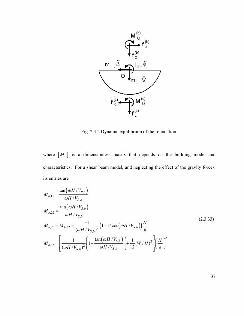
Fig. 2.4.2 Dynamic equilibrium of the foundation.

where [ b ]M is a dimensionless matrix that depends on the building model and

characteristics. For a shear beam model, and neglecting the effect of the gravity forces,

its entries are

( )

( )

( )( )

( )

,

,11,

,

,22,

,23 ,32 ,2,

2, 2

,33 2,,

tan /

/

tan /

/

11 1/ cos /

( / )

tan /1 11 ( /

/ 12( / )

P b

b

P b

S b

b

S b

b b S b

S b

S b

b

S bS b

H VM

H V

H VM

H V

HM M H V

aH V

H V HM W

H V aH V

ω

ω

ω

ω

ωω

ω

ωω

=

=

−= = −

⎡ ⎤⎛ ⎞ ⎛ ⎞⎢ ⎥⎜ ⎟= − + ⎜ ⎟⎜ ⎟⎢ ⎥ ⎝ ⎠⎝ ⎠⎣ ⎦)H

(2.3.33)

37

In eqns (2.3.32) and (2.3.33), is the mass per unit length of the beam, and bm H and

are its height and width, and and W ,S bV ,P bV are its S and P wave velocities. The

dynamic equilibrium of forces acting onto the foundation implies

[ ] [ ]2 (s) ( ) 2fnd fnd b bdriv 2 s

m M K m Mω µ ω⎡ ⎤− − + =⎣ ⎦∆ F ∆ 0∆ (2.3.34)

where is the mass of the foundation, fndm [ ]fndM is the foundation dimensionless mass

matrix

[ ]fnd

2fnd,0 fnd

1 0 0

0 1 0

0 0 /( )

M

I m a

⎡ ⎤⎢ ⎥

= ⎢⎢ ⎥⎢ ⎥⎣ ⎦

⎥ (2.3.35)

where

( )2

2fnd 31fnd,0 0 0 0 02 2

0 0 0

cos sin cossin cos

b mI θ θ θ

θ θ θ⎡ ⎤= + −⎣ ⎦−

θ (2.3.36)

is the mass moment of inertia of the foundation relative to point O, and is the mass

per unit length of the foundation. Finally, one can solve for by inverting a

fndm

∆ 3 3×

matrix

[ ] [ ]1

2 2( ) (s)fnd b

fnd b driv22 2

sm mM M K

ω ωµ

µ µ

−⎡ ⎤

⎡ ⎤= + −⎢ ⎣ ⎦⎢ ⎥⎣ ⎦∆ F⎥ (2.3.37)

For the purpose of brevity, and without loss of generality, the dynamic moments of the

gravity forces were neglected in the above derivations. The expressions including these

moments can be found in Todorovska (1993a,b).

38

2.5 The Free-Field Motion

This section deals with the representation of the free-field motion for incident plane

P-wave, incident plane SV-wave, and for a Rayleigh wave in a fully saturated porous

half-space, considering the effects of the seepage force (which leads to complex valued

and frequency dependent wave velocity in the mixture). The coefficients of the reflected

waves of the P- and S-wave potentials of the Rayleigh waves are derived for open

(permeable) and sealed (impermeable) hydraulic condition on the half-space boundary,

for which the zero stress condition on the half-space surface is Deresiewicz (1960)

0

0

0

0

yy

xy

y

ττσ

=

⎧ ⎫ ⎧ ⎫⎪ ⎪ ⎪ ⎪=⎨ ⎬ ⎨ ⎬⎪ ⎪ ⎪ ⎪⎩ ⎭ ⎩ ⎭

open (permeable) boundary (2.4.1)

and

0

0

0

0

yy

xy

y y yu U

τ στ

+

=

⎧ ⎫ ⎧ ⎫⎪ ⎪ ⎪ ⎪=⎨ ⎬ ⎨⎪ ⎪ ⎪− ⎩ ⎭⎩ ⎭

⎬⎪

sealed (impermeable) boundary (2.4.2)

For incident plane waves (P and SV), the derivation presented in this section, which

is for the genral dissipative case, follows Deresiewicz and Rice (1962). For the Rayleigh

waves, and nondissipative case, the derivation follows Lin et al. (2005).

39

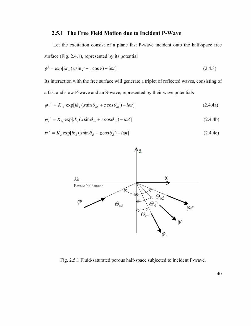
2.5.1 The Free Field Motion due to Incident P-Wave

Let the excitation consist of a plane fast P-wave incident onto the half-space free

surface (Fig. 2.4.1), represented by its potential

])cossin(exp[ tizxii ωγγκφ α −−= (2.4.3)

Its interaction with the free surface will generate a triplet of reflected waves, consisting of

a fast and slow P-wave and an S-wave, represented by their wave potentials

])cossin(exp[1 tizxikK ffff

r

f ωθθϕ αα −+= (2.4.4a)

])cossin(exp[1 tizxikK ssss

r

s ωθθϕ αα −+= (2.4.4b)

])cossin(exp[2 tizxikKr ωθθψ βββ −+= (2.4.4c)

40

Fig. 2.5.1 Fluid-saturated porous half-space subjected to incident P-wave.

where

fk the complex wave number of the fast plane P-wave

sk the complex wave number of the slow plane P-wave

βk the complex wave number of the shear plane wave

We recall that the wave numbers are in general complex, when the dissipation forces due

to the seepage force are considered. These wave numbers can be written in terms of

their real and imaginary parts as

41

kij krk iη η= − , , ,j f s β= (2.4.5)

To ensure dissipation at infinity ki

η in eqn (2.4.3) should be positive. In this work, the

angles of incident wave and of the reflected waves are taken as in H. Deresiewicz and

Rice (1962)

( ) ( ) ( )

sinarc tan

sgn

k kr kj k k

lr l li l l

kp q n

η θθη η

=−

(2.4.6)

where

k

jθ is the reflection angle,

kθ the incident angle, and ,and

kr liη η are the real and imaginary

parts of the wave numbers.

( )

2 2sink kr li ki lr

l

lr li

n k

η η η η θη η

−=

+ (2.4.7)

The reflection angle sine and cosine for the case of l k≠ can be written as

( ) ( ) ( )

1sin k k

l lm in= + k

l (2.4.8)

42

k( ) ( ) ( ) ( )

3cos sgnk k k

l l l lp iq n= (2.4.9)

where

( )

2 2sink kr lr ki li

l

lr li

m k

η η η η θη η

+=

+ (2.4.10)

( ) ( )1

22 2( ) ( ) ( ) ( ) ( )1

,2

k k k k k

l l l l lp q K L K⎡= + ±⎢⎣ ⎦

⎤⎥

k

l

k

l

⎧ ⎫⎪⎬⎪

⎩ ⎭

⎧ ⎫

, (2.4.11)

( ) ( )2 2( ) ( ) ( )1k k

l lK m n= − + (2.4.12a)

and

( ) ( ) ( )2k k

l lL m n= (2.4.12b)

To determine the reflection coefficients both boundary conditions at the free surface are

taken (open boundary and sealed boundary condition):

For open (permeable) half-space surface, the zero stress condition implies

11,1 11,2 12 1 11,1

21,1 21,2 22 1 0 21,1

61,1 61,2 2 61,10

f

s

G G G K G

G G G K a G

G G K G

⎡ ⎤− ⎧ ⎫⎪ ⎪ ⎪⎢ ⎥− − = −⎨ ⎬ ⎨⎢ ⎥⎪ ⎪ ⎪⎢ ⎥ ⎩ ⎭⎣ ⎦

(2.4.13)

and for sealed (impermeable) half-space surface

11,1 61,1 11,2 61,2 12 1 11,1 61,1

21,1 21,2 22 1 0 21,1

1 41,1 2 41,2 3 42 2 1 41,1(1 ) (1 ) (1 ) (1 )

f

s

G G G G G K G G

G G G K a G

f G f G f G K f G

⎡ ⎤+ + − +⎧ ⎫⎪ ⎪ ⎪⎢ ⎥− − = − ⎪⎨ ⎬ ⎨⎢ ⎥ ⎬⎪ ⎪ ⎪⎢ ⎥− − − − − −⎩ ⎭⎣ ⎦

⎪⎩ ⎭

(2.4.14)

where

)sin2( 2

1

2

1,11 ff MkG αα θ−−= (2.4.15a)

)sin2( 2

2

2

2,11 ss MkG αα θ−−= (2.4.15b)

ββ θ2sin2

12 kG = (2.4.15c)

ffkG αα θ2sin2

1,21 −= (2.4.15d)

sskG αα θ2sin2

2,21 −= (2.4.15e)

ββ θ2cos2

22 kG −= (2.4.15f)

ffikG αα θcos1,41 = (2.4.15g)

ssikG αα θcos2,41 = (2.4.15h)

ββ θsin42 ikG −= (2.4.15i)

1

2

1,61 SkG fα−= (2.4.15j)

2

2

2,61 SkG sα−= (2.4.15k)

2.5.2 The Free Field Motion due to Incident SV-Wave

Similarly as for the fast incident P-wave, an incident SV wave can be represented by

its potential

exp[ ( sin cos ) ]ii x z i tαψ κ γ γ= − ω− (2.4.16)

and the interaction with the free-surface will generate the reflected fast and slow P-wave

and an SV-wave, represented by their potentials

])cossin(exp[1 tizxikK ffff

r

f ωθθϕ αα −+= (2.4.17)

])cossin(exp[1 tizxikK ssss

r

s ωθθϕ αα −+= (2.4.18)

43

])cossin(exp[2 tizxikKr ωθθψ βββ −+= (2.4.19)

The critical angle for the fast P-wave is

1sin / 2cr

P Q Rθ µ−= + + (2.4.20)

The zero stress condition for open (permeable) half-space surface implies

11,1 11,2 12 1 12

21,1 21,2 22 1 0 22

61,1 61,2 20 0

f

s

G G G K G

G G G K b G

G G K

∗

∗

⎧ ⎫⎡ ⎤− ⎧ ⎫⎪ ⎪⎪ ⎪⎢ ⎥− − = −⎨ ⎬ ⎨⎢ ⎥

⎪ ⎪ ⎪⎢ ⎥ ⎩ ⎭⎣ ⎦ ⎩ ⎭

⎬⎪

(2.4.21)

and for sealed (impermeable) half-space surface it implies

11,1 61,1 11,2 61,2 12 1 12

21,1 21,2 22 1 0 22

1 41,1 2 41,2 3 42 2 3 42(1 ) (1 ) (1 ) (1 )

f

s

G G G G G K G

G G G K b G

f G f G f G K f G

∗

∗

∗

⎧ ⎫⎡ ⎤+ + − ⎧ ⎫⎪ ⎪⎪ ⎪⎢ ⎥− − = −⎨ ⎬ ⎨⎢ ⎥ ⎬

⎪ ⎪ ⎪⎢ ⎥− − − − − −⎩ ⎭⎣ ⎦ ⎩ ⎭⎪

(2.4.22)

2.5.3 The Free Field Motion due to Rayleigh-Wave

A Rayleigh in the half-space propagating in the positive x- direction can be

represented by its potentials

( )1 fb y i kx t

f fc e e

ωφ − −=

( )1si kx tb y

s sc e e

ωφ −−= (2.4.23)

( )2i kx tb y

De eωψ −−=

where

2

1 21f

f

cb k

Vα

= − (2.4.24a)

44

2

1 21

s

s

cb k

Vα

= − (2.4.24b)

2

2 21

cb k

Vβ

= − (2.4.24c)

The zero stress condition for open (permeable) half-space surface implies

11,1 11,2 12 1

21,1 21,2 22 1

61,1 61,2

0

0

0 0

f

s

G G G b

G G G b

G G D

∗∗ ∗∗ ∗∗

∗∗ ∗∗ ∗∗

∗∗ ∗∗

⎡ ⎤− ⎧ ⎫ ⎧ ⎫⎢ ⎥ ⎪ ⎪ ⎪ ⎪− − =⎨ ⎬ ⎨ ⎬⎢ ⎥

⎪ ⎪ ⎪ ⎪⎢ ⎥ ⎩ ⎭ ⎩ ⎭⎣ ⎦

(2.4.25)

and for sealed (impermeable) half-space surface it implies

11,1 61,1 11,2 61,2 12 1

21,1 21,2 22 1

1 41,1 2 41,2 3 42

0

0

(1 ) (1 ) (1 ) 0

f

s

G G G G G b

G G G b

f G f G f G D

∗∗ ∗∗ ∗∗ ∗ ∗∗

∗∗ ∗∗ ∗∗

∗∗ ∗∗ ∗∗

⎡ ⎤+ + − ⎧ ⎫ ⎧ ⎫⎢ ⎥ ⎪ ⎪ ⎪ ⎪− − =⎨ ⎬ ⎨ ⎬⎢ ⎥

⎪ ⎪ ⎪ ⎪⎢ ⎥− − − − − ⎩ ⎭ ⎩ ⎭⎣ ⎦

(2.4.26)

where

2 22 1

11,1 22

f

k c MG k

Vα

∗∗ = − (2.4.27a)

2 22 2

11,2 22

s

k c MG k

Vα

∗∗ = − (2.4.27b)

22

12 22 1

cG ik

Vβ

∗∗ = − − (2.4.27c)

22

21,1 22 1

f

cG ik

Vα

∗∗ = − (2.4.27d)

45

22

21,2 22 1

s

cG ik

Vα

∗∗ = − (2.4.27e)

2 22

22 22

k cG k

Vβ

∗∗ = − (2.4.27f)

2 2

161,1 2

f

S k cG

Vα

∗∗ = − (2.4.27g)

2 2

261,2 2

s

S k cG

Vα

∗∗ = − (2.4.27h)

For a nontrivial solution, the determinate of the matrices in eqns (2.4.25) and (2.4.26)

have to be equal to zero, which gives for open (permeable) half-space surface

( ) ( ) ( )

( )

2 2 2 2 2 2 2 2

2 1 1 2 1 2 2 1

2 2 2 24 2 2 2 2

1 2 2 1 2 12 2 2 2

det 4 2 2

4 1 1 4 1 1

f s s f

f s

f s s s

S V S V V S V S V c S M S M V c

c c c cM S M S c S V V S V V

V V V V

α α β α α β

α β α βα α α α

= − + − + −

+ − − − − + − − 0=

(4.2.28)

and for sealed (impermeable) half-space surface

46

( )( ) ( )

( )( ) ( )( )

( )( ) ( )

2 2 2 2 2 2

12 2 2 2 2 22

3 1 2 2 2 2 4 2

1 2

2 2 2 2 2 2 4 2

3 1 2 1 1

2

2 2 2 2 2 2

3 2 1

4 21 4 2 1

2det 1

1 2 1 2

41 4 2 1

f s s

f s s

f s s

s

s s s

f s

f s f

V V V c M V Vf V V V c M V V f c

c V V c M VV

f S c V V f S c V V S c V

V Vf V V V c M V V f

α α β α βα α β α β

α α αα

α β α β α

α αα α β α β

⎡ ⎤⎛ ⎞− −⎢ ⎥⎜ ⎟− − − + −

⎜ ⎟+⎢ ⎥= −⎝ ⎠⎢ ⎥+ − + − − +⎢ ⎥⎣ ⎦

− − + −+

( )( ) ( )( )

( )

2 2 2 2 2

22

2 2 2 4 2

2 2

2 2 2 2 2 2 4 2

3 2 1 2 2

2 2 22 2 2

2 1 2 2 2

2

2 1

1 2 1 2

4 1 1 1 0

f

f s f

f

f s f

f s

f s

V c M V V

cc V V c M V

Vf S c V V f S c V V S c V

c c cf f V V V

V V V

β α β

α α αα

α β α β α

α α βα α β

⎡ ⎤⎛ ⎞− −⎢ ⎥⎜ ⎟

⎜ ⎟+⎢ ⎥ −⎝ ⎠⎢ ⎥− − − − − +⎢ ⎥⎣ ⎦

⎡ ⎤+ − − − − =⎣ ⎦

(2.4.29)

Equations (2.4.28) and (2.4.29) are the characteristic equations the solution of which

gives the allowable phase velocities of Rayleigh waves, , for both conditions. Then by

substituting the corresponding velocity in eqns (4.2.25) and (4.2.26), the coefficients of

the wave potentials can be determined.

c

47

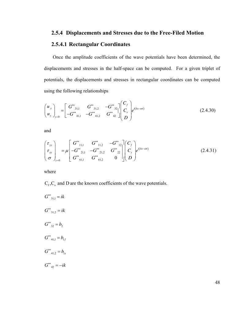
2.5.4 Displacements and Stresses due to the Free-Filed Motion

2.5.4.1 Rectangular Coordinates

Once the amplitude coefficients of the wave potentials have been determined, the

displacements and stresses in the half-space can be computed. For a given triplet of

potentials, the displacements and stresses in rectangular coordinates can be computed

using the following relationships

48

)(31,1 31,2 32

41,1 41,2 420

f

x i kx t

s

y y

Cu G G G

C eu G G G

D

ω∗∗ ∗∗ ∗∗

−∗∗ ∗∗ ∗∗

=

⎛ ⎞⎡ ⎤−⎛ ⎞ ⎜ ⎟= ⎢ ⎥⎜ ⎟ ⎜ ⎟− −⎝ ⎠ ⎣ ⎦ ⎜ ⎟

⎝ ⎠

(2.4.30)

and

(11,1 11,2 12

21,1 21,2 22

61,1 61,200

yy f

i kx t

xy s

y

G G G C

G G G C e

G G D

)ω

ττ µσ

∗∗ ∗∗ ∗∗

−∗∗ ∗∗ ∗∗

∗∗ ∗∗=

⎡ ⎤−⎛ ⎞ ⎛ ⎞⎢ ⎥⎜ ⎟ ⎜ ⎟= − −⎢ ⎥⎜ ⎟ ⎜ ⎟

⎜ ⎟ ⎜ ⎟⎢ ⎥⎝ ⎠ ⎝ ⎠⎣ ⎦

(2.4.31)

where

f sC ,C and D are the known coefficients of the wave potentials.

31,1G i∗∗ = k

k

31,2G i∗∗ =

32 2G b∗∗ =

41,1 1 fG b∗∗ =

41,2 1sG b∗∗ =

42G i∗∗ = − k

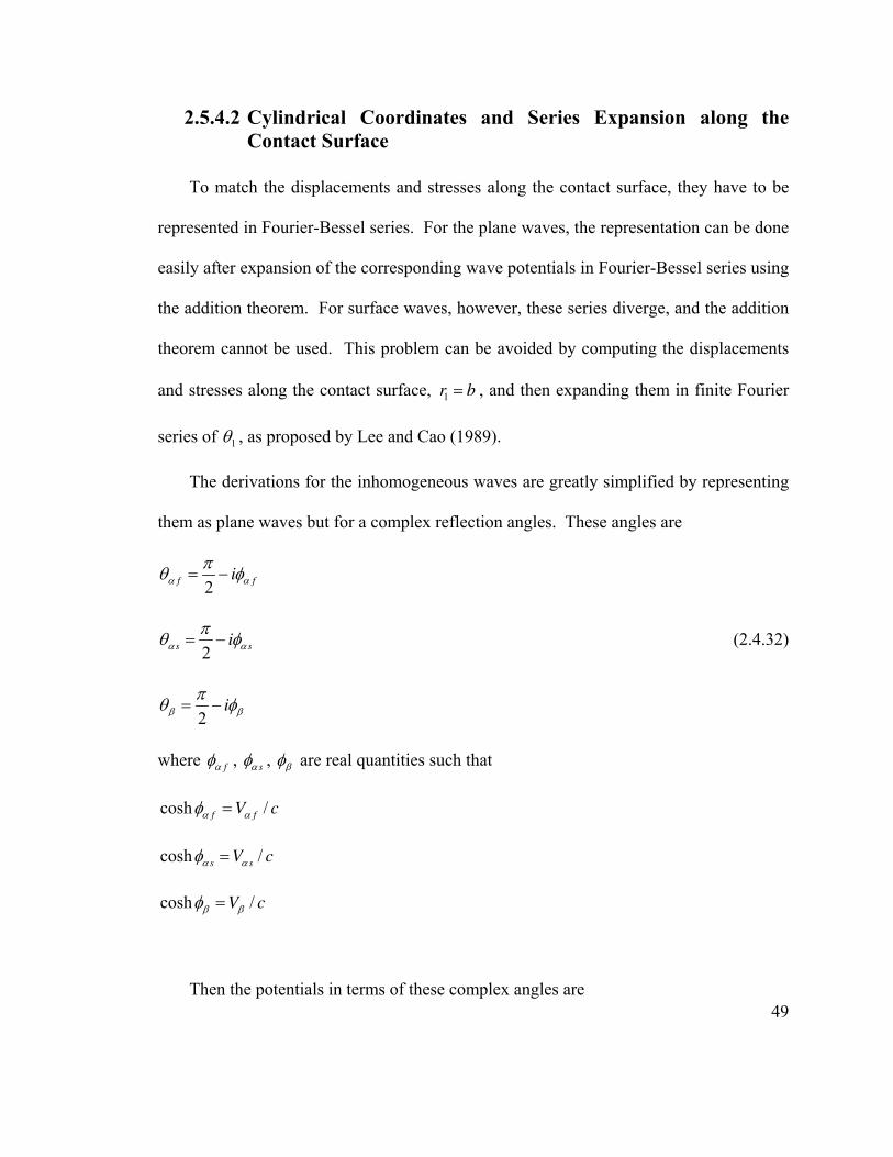
2.5.4.2 Cylindrical Coordinates and Series Expansion along the

Contact Surface

To match the displacements and stresses along the contact surface, they have to be

represented in Fourier-Bessel series. For the plane waves, the representation can be done

easily after expansion of the corresponding wave potentials in Fourier-Bessel series using

the addition theorem. For surface waves, however, these series diverge, and the addition

theorem cannot be used. This problem can be avoided by computing the displacements

and stresses along the contact surface, 1r b= , and then expanding them in finite Fourier

series of 1θ , as proposed by Lee and Cao (1989).

The derivations for the inhomogeneous waves are greatly simplified by representing

them as plane waves but for a complex reflection angles. These angles are

2f fiα α

πθ φ= −

2s siα α

πθ φ= − (2.4.32)

2iβ β

πθ φ= −

where fαφ ,

sαφ , βφ are real quantities such that

cosh /f f

V cα αφ =

cosh /s s

V cα αφ =

cosh /V cβ βφ =

49

Then the potentials in terms of these complex angles are

( )( )1 11cosf ff

ik r i tb d

f fC e eα αθ θ ωφ − −

=

( )( )1 11coss ss

ik r i tb d

s sC e e α αθ θ ωφ − −= (2.4.33)

( )( )1 12cosik r i tb d

De eβ βθ θ ωψ − −

=

Displacements and stresses can be computed in cylindrical coordinates from the

potentials using the following relationships

1

1 1

1j

ru

r r 1

φ ψθ

∂ ∂= +∂ ∂

(2.4.34a)

1

1 1 1

1 ju

r rθ

φ ψθ∂ ∂

= −∂ ∂

(2.4.34b)

and

1 1 1 1 1 1

1 1

11 1 1 1 1 1 1 1

1 12

r r r r

r r

r

u u u U U U uQ

r r r r r r

θ θτ λ µθ θ

⎛ ⎞∂ ∂ ∂ ∂⎛ ⎞= + + + + + +⎜ ⎟⎜ ⎟ ⎜ ⎟∂ ∂ ∂ ∂⎝ ⎠ ⎝ ⎠

1r∂

∂ (2.4.35a)

1 1 1

1 1

1 1 1 1

1 r

r

u u u

r r r

θ θθτ µ

θ∂ ∂⎛ ⎞

= + +⎜ ∂ ∂⎝ ⎠⎟ (2.4.35b)

This gives for the displacements along the canyon rim 1r b= and for 0 0θ θ θ− ≤ ≤

( )( ) ( )

( )1

1 1

1

1

cos cos1,

sin

f sA A

f f f s s s i t

r A

C ik b e C ik b eu b e

b Dik b e β

α α α α ω

β β

θ θ θ θθ

θ θ−

⎡ ⎤− + − −⎢ ⎥=⎢ ⎥−⎣ ⎦

(2.4.36a)

( )( ) ( )

( )1

1 1

1

1

sin sin1,

cos

f sA A

f f f s s s i t

A

C ik b e C ik b eu b e

b Dik b e β

α α α α ωθ

β β

θ θ θ θθ

θ θ−

⎡ ⎤− − − −⎢ ⎥=⎢ ⎥−⎣ ⎦

− (2.4.36b)

for the solid,

50

( )( ) ( )

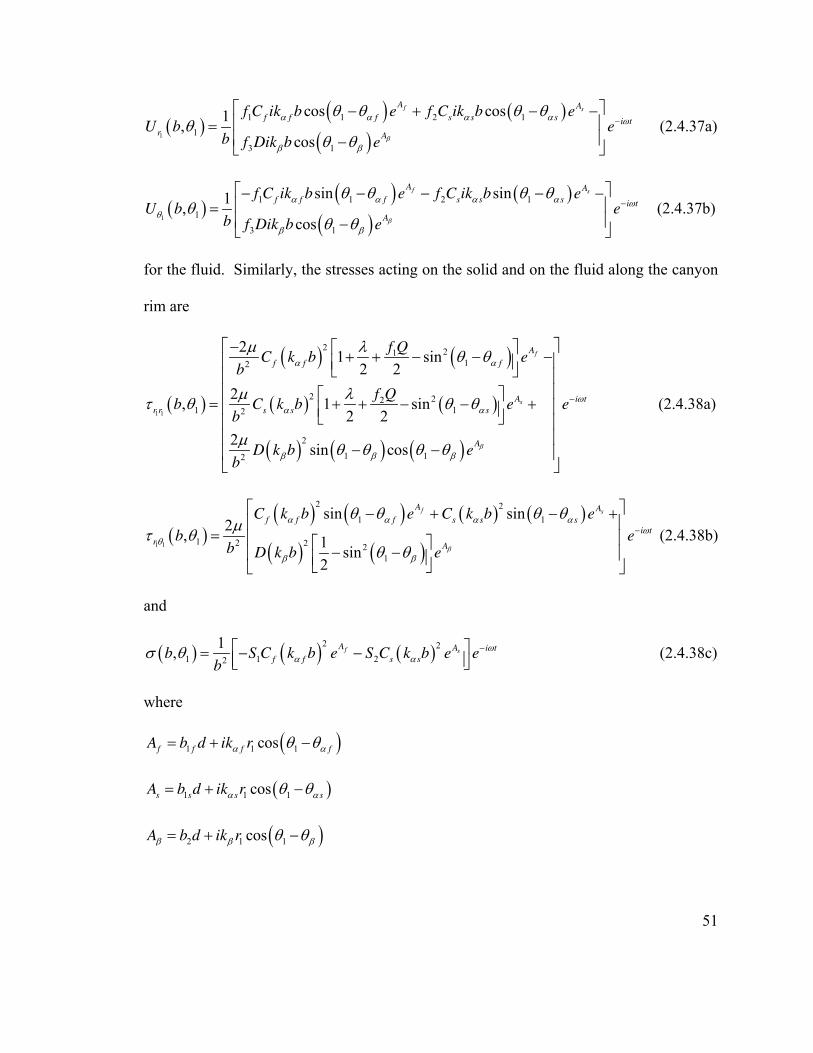
( )1

1 1 2 1

1

3 1

cos cos1,

cos

f sA A

f f f s s s i t

r A

f C ik b e f C ik b eU b e

b f Dik b e β

α α α α ω

β β

θ θ θ θθ

θ θ−

⎡ ⎤− + − −⎢ ⎥=⎢ ⎥−⎣ ⎦

(2.4.37a)

( )( ) ( )

( )1

1 1 2 1

1

3 1

sin sin1,

cos

f sA A

f f f s s s i t

A

f C ik b e f C ik b eU b e

b f Dik b e β

α α α α ωθ

β β

θ θ θ θθ

θ θ−

⎡ ⎤− − − −⎢ ⎥=⎢ ⎥−⎣ ⎦

− (2.4.37b)

for the fluid. Similarly, the stresses acting on the solid and on the fluid along the canyon

rim are

( )

( ) ( )

( ) ( )

( ) ( ) ( )

1 1

221

12

2 221 12

2

1 12

21 sin

2 2

2, 1 sin

2 2

2sin cos

f

s

A

f f f

A i t

r r s s s

A

f QC k b e

b

f Qb C k b e

b

D k b eb

β

α α

eω

α α

β β β

µ λ θ θ

µ λτ θ θ θ

µ θ θ θ θ

−

⎡ ⎤− ⎡ ⎤+ + − − −⎢ ⎥⎢ ⎥⎣ ⎦⎢ ⎥⎢ ⎥⎡ ⎤= + + − − +⎢ ⎥⎢ ⎥⎣ ⎦⎢ ⎥⎢ ⎥

− −⎢ ⎥⎣ ⎦

(2.4.38a)

( )( ) ( ) ( ) ( )

( ) ( )1 1

2 2

1 1

1 2 2 2

1

sin sin2

, 1sin

2

f sA A

f f f s s s

i t

rA

C k b e C k b e

b eb D k b e β

α α α αω

θ

β β

θ θ θ θµτ θ

θ θ−

⎡ ⎤− + − +⎢ ⎥

= ⎢ ⎥⎡ ⎤− −⎢ ⎥⎢ ⎥⎣ ⎦⎣ ⎦

(2.4.38b)

and

( ) ( ) ( )2 2

1 1 22

1, f s

A A i t

f f s sb S C k b e S C k b eb

eω

α ασ θ −⎡= − −⎢⎣⎤⎥⎦

(2.4.38c)

where

( )1 1 1cosf f f fA b d ik rα αθ θ= + −

( )1 1 1coss s s

A b d ik rα α sθ θ= + −

( )2 1 1cosA b d ik rβ β βθ θ= + −

51

Chapter 3: Numerical Results and Analysis

This chapter presents numerical results for: the wave velocities, free-field motion,

foundation input motion, foundation stiffness and damping, and system response in the

form of a parametric study, with the objective of understanding the effects of the many

model parameters. The following Chapter 6 shows results for a model with properties

similar to those for Millikan library, attempting to explain the observed effects.

The results were computed using a FORTRAN computer program SSI_POROUS

(Todorovska and Al Rjoub, 2006a), which was generalized to work for a dissipative

medium (i.e. for a mixture that has finite permeability and is saturated with viscous

fluid), and for partially saturated soils. This generalization required computation of

Bessel functions of complex arguments, and subroutines from Zhang and Jin (1996) were

used. The computer program was written in terms of dimensionless parameters, defined

using as reference: length a , material modulus sµ , and mass density grρ . Then, the

system response is a function of the following dimensionless parameters: stiffness of the

fluid relative to the skeleton, defined through the ratio /f sK µ and the Poisson’s ratio sν ;

mass density of the skeleton relative to the fluid, defined through the ratio gr / fρ ρ and

the porosity ; mass of the building relative to the mass of the foundation, and mass of

the foundation relative to the mass of the replaced soil, through the ratios

n̂

b fnd/m m and

, where, fnd gr/m m gr fnd grm A ρ=

)

is the mass of the excavated soil (per unit length) if there

were no voids, and is the area of the foundation; the flexibility of the building

relative to that of the soil, through the ratio

fndA

ref ,b( ) /( SV H V aε =

52

[ ],b ref( ) / / ( ) /SH V a Vω ω⎡ ⎤= ⎣ ⎦ = ratio of the number of wavelength in the shear beam in

length H and the number of reference wavelengths in the soil in length a; dimensionless

frequency ref/( )a Vη ω π= , where ref gr/sV µ ρ= is a reference velocity; foundation

shape, through the ratio ; and on the type, amplitude and angle of the incident waves. /h a

3.1 Soil Constitutive Properties and Waves Velocities

The wave velocities in the soil and the frequency of motion are fundamental for

significance of the effects of the soil-structure interaction. When the effects of the

seepage force are considered, the wave velocities depend themselves on the degree of

dissipation and also on frequency. Hence, the analysis begins with understanding how

the wave velocities depend on frequency and on the soil permeability (for fixed value of

viscosity of the fluid), which will help later on, interpret the results for the foundation

stiffness and damping.

3.1.1 Input Model Parameters

The following range of the input parameters was considered in the analysis. The pore

fluid in this study is water, which has mass density kg/m310wρ = 3 and bulk modulus

Pa, giving bulk wave velocity 92.2 10wK = × /w wK ρ =1,483 m/s. For full saturation,

f wK K= and f wρ ρ= . For the mass density of the material of which the grain is made

value was used. The ratio 3gr 2.7 10 kg/mρ = × 3 / fKµ , where f wK K= describes the

stiffness of the skeleton, which is varied so that / fKµ = 0.01, 0.1, 1, and 10. The value

/ fKµ = 0.01 corresponds to soft soil, / fKµ = 0.1 to stiff soil, and / fKµ = 1 and 10 to

53

porous rock (Lin et al., 2001). Only one value of Poisson ratio is considered, sν =0.3, and

two values of porosity, n =0.3 and 0.4, which are representative for soils. The

dissipation depends on the ratio ˆˆ / kµ , where µ̂ is the absolute viscosity of the fluid, and

is the intrinsic permeability of the skeleton. The absolute viscosity of water at about

25 C is

k̂

° ˆwµ = -30.89 10× Pa s⋅ (1 Pa s⋅ =1 ). In this work, a rounded value

is used. The intrinsic permeability of the skeleton depends on the

type of geologic material. Pervious consolidated geo materials, such as highly fractured

rock, and pervious unconsolidated geo materials such as well-sorted gravel and well-

sorted sand and gravel, have intrinsic permeability in the range 10 .

Semi-pervious consolidated geo materials, such as oil reservoir rocks and fresh

sandstone, and semi-pervious unconsolidated geo materials, such as very find sand, silt,

loess and loam, have in the range

2N s/m

3ˆ ˆ 10wµ µ −= = 2N s/m

k̂ 6 1010− −− 2m

k̂ 11 1410 10− −− 2m (Bear, 1972). Geo materials with

in the range are considered to be impervious. In this work, results are

shown for , and also for the case when the effects of the dissipative force

are neglected, and the wave velocities are real values (this case is referred to as the “no

seepage force” or the “ ” case). For dry soil (pores filled with air), the following

values are taken:

k̂ 15 1910 10− − 2m−

−12 6ˆ10 10k− ≤ ≤

k̂ →∞

gr / fρ ρ =0.001 and /fK sµ =0.001, and the dry shear wave velocity is

computed as ,dry grˆ/[(1 ) ]S sV nµ ρ= − . Another variable of the model is the frequency

of motion.

54

The upper bound of frequency is constrained by the requirements that: (1) the flow of

the fluid in the pores is laminar, and (2) the wavelengths are much larger than the size of

the pores. The first requirement implies frequency bound 2

ˆ

4tf

d

πν= , where d is the

diameter of the pores, and ν̂ is the kinematic viscosity, which is related to the dynamic

viscosity µ̂ and fluid density fρ by ˆ ˆ / fν µ ρ= (Biot, 1956a). This implies maximum

frequencies Hz for 10,000tf = 0.01d = mm (silt), 100tf = Hz for mm (sands),

and Hz for mm (coarse sands to gravel). We consider frequencies not

larger than 100 Hz in presenting results for the wave velocities and free-field motions,

and dimensionless frequency

0.1d =

10tf = 1d =

5η ≤ , where ref ref/( ) (2 ) /a V a f Vη ω π= = , and

, and is the characteristic dimension for the wave scattering problem and

radiation problem. Then for the softest soils considered (

ref S,dryV V= 2a

/ fKµ =0.01), for which the

smallest wave velocity is of the order of 100 m/s, and for =24 m, which is the value

used for the case study (Millikan library), the maximum value of

2a

5η = implies highest

frequency Hz, which is low enough for the flow to be laminar. 20f =

3.1.2 Wave Velocities for Full Saturation as Function of the Model

Parameters

For very small ˆ ˆ1

ˆ

n

k

µω

, which has dimension of mass density, the seepage force is much

smaller than the inertial forces, and its effects are negligible (see eqns (2.2.7c,d)). In that

case, the wave velocities are real valued, do not depend on frequency, and are used in this

55

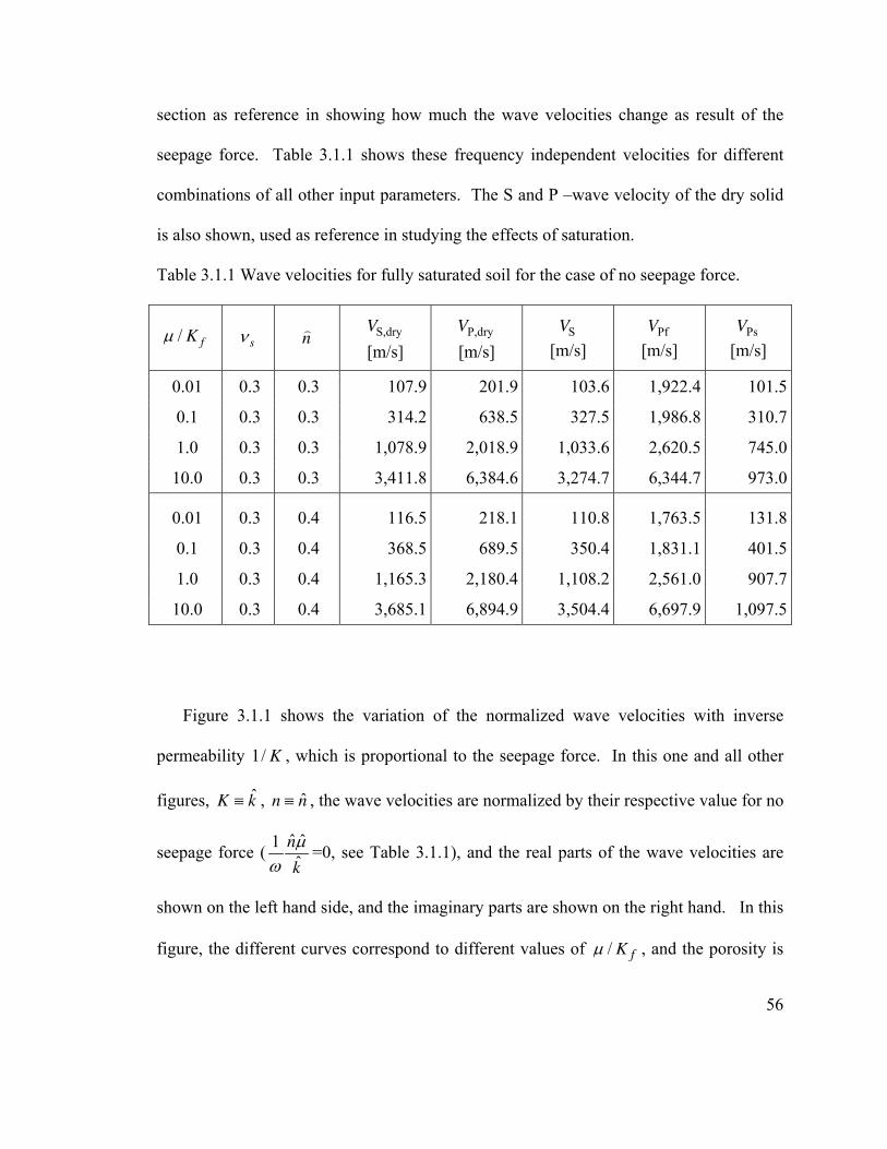
section as reference in showing how much the wave velocities change as result of the

seepage force. Table 3.1.1 shows these frequency independent velocities for different

combinations of all other input parameters. The S and P –wave velocity of the dry solid

is also shown, used as reference in studying the effects of saturation.

Table 3.1.1 Wave velocities for fully saturated soil for the case of no seepage force.

/ fKµ sν n S,dryV

[m/s]

P,dryV

[m/s]

SV

[m/s]

PfV

[m/s]

PsV

[m/s]

0.01 0.3 0.3 107.9 201.9 103.6 1,922.4 101.5

0.1 0.3 0.3 314.2 638.5 327.5 1,986.8 310.7

1.0 0.3 0.3 1,078.9 2,018.9 1,033.6 2,620.5 745.0

10.0 0.3 0.3 3,411.8 6,384.6 3,274.7 6,344.7 973.0

0.01 0.3 0.4 116.5 218.1 110.8 1,763.5 131.8

0.1 0.3 0.4 368.5 689.5 350.4 1,831.1 401.5

1.0 0.3 0.4 1,165.3 2,180.4 1,108.2 2,561.0 907.7

10.0 0.3 0.4 3,685.1 6,894.9 3,504.4 6,697.9 1,097.5

Figure 3.1.1 shows the variation of the normalized wave velocities with inverse

permeability , which is proportional to the seepage force. In this one and all other

figures, , , the wave velocities are normalized by their respective value for no

seepage force (

1/ K

ˆK k≡ ˆn n≡

ˆ ˆ1

ˆ

n

k

µω

=0, see Table 3.1.1), and the real parts of the wave velocities are

shown on the left hand side, and the imaginary parts are shown on the right hand. In this

figure, the different curves correspond to different values of / fKµ , and the porosity is

56

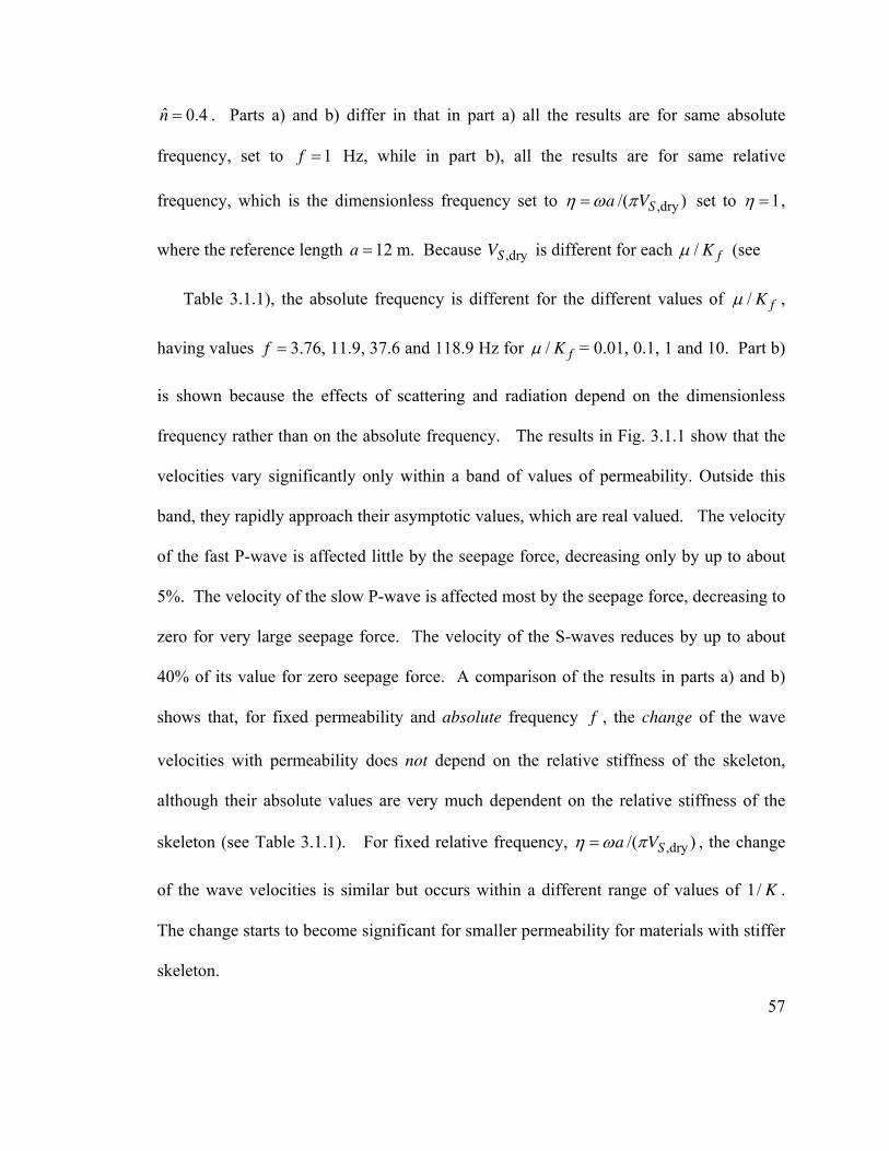
ˆ 0.4n = . Parts a) and b) differ in that in part a) all the results are for same absolute

frequency, set to 1f = Hz, while in part b), all the results are for same relative

frequency, which is the dimensionless frequency set to ,dry/( )Sa Vη ω π= set to 1η = ,

where the reference length a =12 m. Because is different for each ,drySV / fKµ (see

Table 3.1.1), the absolute frequency is different for the different values of / fKµ ,

having values f = 3.76, 11.9, 37.6 and 118.9 Hz for / fKµ = 0.01, 0.1, 1 and 10. Part b)

is shown because the effects of scattering and radiation depend on the dimensionless

frequency rather than on the absolute frequency. The results in Fig. 3.1.1 show that the

velocities vary significantly only within a band of values of permeability. Outside this

band, they rapidly approach their asymptotic values, which are real valued. The velocity

of the fast P-wave is affected little by the seepage force, decreasing only by up to about

5%. The velocity of the slow P-wave is affected most by the seepage force, decreasing to

zero for very large seepage force. The velocity of the S-waves reduces by up to about

40% of its value for zero seepage force. A comparison of the results in parts a) and b)

shows that, for fixed permeability and absolute frequency f , the change of the wave

velocities with permeability does not depend on the relative stiffness of the skeleton,

although their absolute values are very much dependent on the relative stiffness of the

skeleton (see Table 3.1.1). For fixed relative frequency, ,dry/( )Sa Vη ω π= , the change

of the wave velocities is similar but occurs within a different range of values of 1/ .

The change starts to become significant for smaller permeability for materials with stiffer

skeleton.

K

57

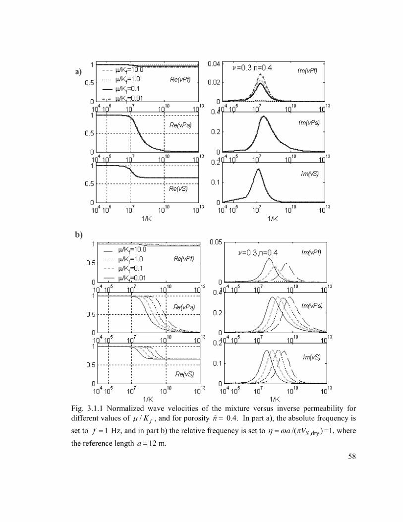
Fig. 3.1.1 Normalized wave velocities of the mixture versus inverse permeability for

different values of / fKµ , and for porosity n̂ = 0.4. In part a), the absolute frequency is

set to 1f = Hz, and in part b) the relative frequency is set to ,dry/( )Sa Vη ω π= =1, where

the reference length 12 m. a =

58

Figure 3.1.2 also shows the variation of the normalized wave velocities with inverse

permeability , but the different curves correspond to different values of frequency

, 1, 10 and 100 Hz. In part a),

1/ K

0.1f = / fKµ =0.1 (stiff soil), in part b) / fKµ =0.01

(soft soil), and in both parts the porosity is n̂ = 0.4. It can be seen from this figure that,

for smaller frequencies of motion, the seepage force starts to affect the wave velocities at

smaller 1/ , i.e. at higher permeability. This trend is as expected, because the effect of

the seepage force is through the combination

K

ˆˆ ˆ /( )n kµ ω .

Fig. 3.1.3 shows the normalized wave velocities versus frequency f in Hz on a

logarithmic scale for different values of inverse permeability 1/ . As in Fig. 3.1.2, in

part a),

K

/ fKµ =0.1 (stiff soil), in part b) / fKµ =0.01 (soft soil), and in both parts the

porosity is 0.4. It can be seen that the trend of the variation of the normalized wave

velocities with increasing frequency is the same as the trend with increasing permeability

(see Fig. 3.1.2), which is due to the fact that in Biot’s theory, the effect of the seepage

force is through the ratio

n̂ =

ˆˆ ˆ /( )n kµ ω .

59

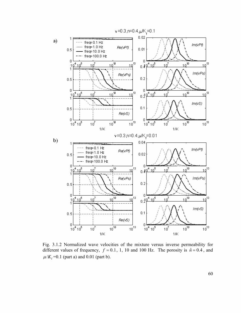
Fig. 3.1.2 Normalized wave velocities of the mixture versus inverse permeability for

different values of frequency, 0.1f = , 1, 10 and 100 Hz. The porosity is , and ˆ 0.4n =

f/Kµ =0.1 (part a) and 0.01 (part b).

60

Fig. 3.1-3 Normalized wave velocities versus frequency for different values of

permeability. The porosity is ˆ 0.4n = , and f/Kµ =0.1 (part a) and 0.01 (part b).

61

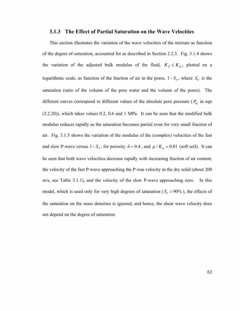
3.1.3 The Effect of Partial Saturation on the Wave Velocities

This section illustrates the variation of the wave velocities of the mixture as function

of the degree of saturation, accounted for as described in Section 2.2.3. Fig. 3.1.4 shows

the variation of the adjusted bulk modulus of the fluid, f wK K≤ , plotted on a

logarithmic scale, as function of the fraction of air in the pores, 1 , where is the

saturation (ratio of the volume of the pore water and the volume of the pores). The

different curves correspond to different values of the absolute pore pressure ( in eqn

(2.2.20)), which takes values 0.2, 0.6 and 1 MPa. It can be seen that the modified bulk

modulus reduces rapidly as the saturation becomes partial even for very small fraction of

air. Fig. 3.1.5 shows the variation of the modulus of the (complex) velocities of the fast

and slow P-wave versus 1 , for porosity

rS− rS

aP

rS− ˆ 0.4n = , and / 0.01wKµ = (soft soil). It can

be seen that both wave velocities decrease rapidly with increasing fraction of air content,

the velocity of the fast P-wave approaching the P-was velocity in the dry solid (about 200

m/s, see Table 3.1.1), and the velocity of the slow P-wave approaching zero. In this

model, which is used only for very high degrees of saturation ( ), the effects of

the saturation on the mass densities is ignored, and hence, the shear wave velocity does

not depend on the degree of saturation.

90%rS >

62

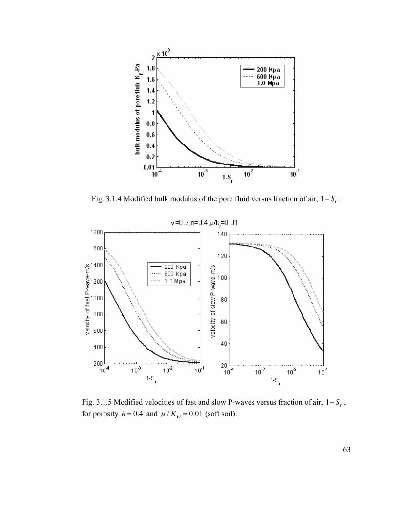
Fig. 3.1.4 Modified bulk modulus of the pore fluid versus fraction of air, 1 rS− .

Fig. 3.1.5 Modified velocities of fast and slow P-waves versus fraction of air, 1 rS− ,

for porosity and ˆ 0.4n = / 0.01wKµ = (soft soil).

63

3.2 Foundation Complex Stiffness Matrix

This section shows results for the real and imaginary part of the foundation

impedance matrix, where the real part describes the foundation stiffness, and the

imaginary part is related to the damping due to radiation of energy from a vibrating

foundation. Section 3.2.1 shows results for fully saturated soils, and Section 3.2.2 for

partially saturated soils. In all figures, the Poisson’s ratio is 0.3ν = , the porosity is

, and the dimensionless frequency is defined with respect to the shear wave

velocity of the dry solid,

ˆ 0.4n =

,s dry

a

V

ωηπ

= , which is independent of the state of saturation.

Results are shown only for “stiff” and “soft” soils, i.e. for / 0.1f

Kµ = and 0.01, because

the effects of the pore water are more significant for solids with relatively soft skeleton.

3.2.1 Foundation Complex Stiffness Matrix for Fully Saturated Soils

Figure 3.2.1 shows results for / 0.1f

Kµ = , for different values of permeability. Part

a) shows results for permeable (open) foundation-soil interface, and part b) for

impermeable (sealed) interface. It is noted here that the hydraulic condition on the half-

space surface does not affect the results, as the effect of the free surface on the scattered

waves from the foundation was neglected in the development of the model. In each part,

the plots on the left show the real part and those on the right show the imaginary part of

the corresponding foundation stiffness matrix coefficient, and the three rows of plots

show respectively (horizontal and vertical stiffness which are equal for this

model for a semi-circular foundation), (rocking stiffness), and (coupling term

11 22= K K

33K 23K

64

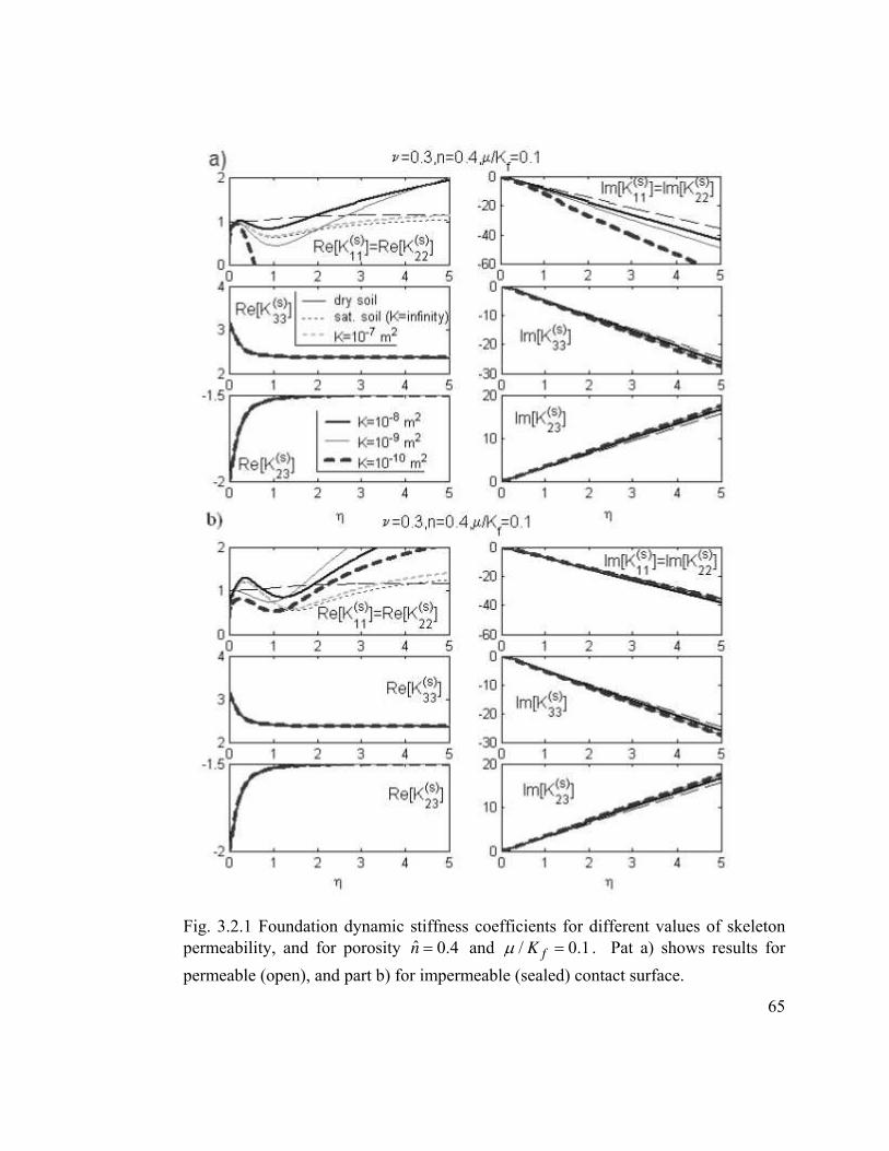
Fig. 3.2.1 Foundation dynamic stiffness coefficients for different values of skeleton

permeability, and for porosity ˆ 0.4n = and / 0fK .1µ = . Pat a) shows results for

permeable (open), and part b) for impermeable (sealed) contact surface.

65

Fig. 3.2.2 Foundation dynamic stiffness coefficients for different values of skeleton

permeability, and for porosity ˆ 0.4n = and / 0.fK 01µ = . Pat a) shows results for

permeable (open), and part b) for impermeable (sealed) contact surface.

66

67

01

between horizontal and rocking motions). Similarly, Fig. 3.2.2 shows results for

/ 0.f

Kµ = (soft soil). The results are discussed in what follows.

A noted in Todorovska and Al Rjoub (2006b) the effect of saturation for this shape

of embedded foundation is such that it affects significantly both the horizontal and the

vertical stiffness, while the effect on the rocking and coupling stiffness coefficients is

very small. This can be explained by the fact that the rocking motion of the foundation

results only in shear deformations in the soil and motion of soil tangent to the contact

surface, which does not cause flow of fluid perpendicular to the foundation-soil interface

(hence pressure from the fluid onto the foundation). What is different in this thesis from

the study in Todorovska and Al Rjoub (2006b) is that the effects of the seepage force are

considered, which, as noted in Section 3.1 lead to complex valued wave velocities in the

soil, and also the effects of partial saturation. Hence, in this thesis work, the emphasis is

on analyzing the effects of finite permeability and partial saturation.

Todorovska and Al Rjoub (2006b) explained the trend of the effect of the pore water

as increasing the stiffness of the foundation for small frequencies for which the water

moves in phase with the solid, but the effects reverses for high enough frequency, when

the pore water moves in the opposite direction of the solid, and it reduces the foundation

stiffness. For very stiff skeleton (e.g. rock) the effect is very small, while for some very

soft soils, the window of frequencies where there would be an increase of stiffness may

be very small for the increase to be noticeable. The presence of a dissipative force is

expected to increase the dynamic stiffness of the foundation. Figures 3.2.1 and 3.2.2

shows that the horizontal and vertical stiffness (real part of ) do increase with 11 22= K K

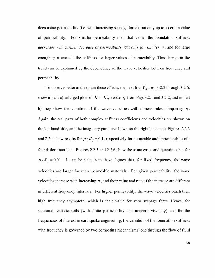
decreasing permeability (i.e. with increasing seepage force), but only up to a certain value

of permeability. For smaller permeability than that value, the foundation stiffness

decreases with further decrease of permeability, but only for smaller η , and for large

enough η it exceeds the stiffness for larger values of permeability. This change in the

trend can be explained by the dependency of the wave velocities both on frequency and

permeability.

To observe better and explain these effects, the next four figures, 3.2.3 through 3.2.6,

show in part a) enlarged plots of versus 11 22= K K η from Figs 3.2.1 and 3.2.2, and in part

b) they show the variation of the wave velocities with dimensionless frequency η .

Again, the real parts of both complex stiffness coefficients and velocities are shown on

the left hand side, and the imaginary parts are shown on the right hand side. Figures 2.2.3

and 2.2.4 show results for / 0.1f

Kµ = , respectively for permeable and impermeable soil-

foundation interface. Figures 2.2.5 and 2.2.6 show the same cases and quantities but for

/ 0.f

K 01µ = . It can be seen from these figures that, for fixed frequency, the wave

velocities are larger for more permeable materials. For given permeability, the wave

velocities increase with increasing η , and their value and rate of the increase are different

in different frequency intervals. For higher permeability, the wave velocities reach their

high frequency asymptote, which is their value for zero seepage force. Hence, for

saturated realistic soils (with finite permeability and nonzero viscosity) and for the

frequencies of interest in earthquake engineering, the variation of the foundation stiffness

with frequency is governed by two competing mechanisms, one through the flow of fluid

68

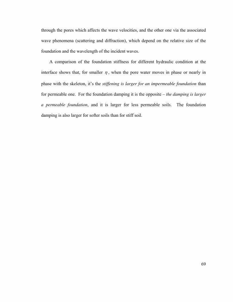
through the pores which affects the wave velocities, and the other one via the associated

wave phenomena (scattering and diffraction), which depend on the relative size of the

foundation and the wavelength of the incident waves.

A comparison of the foundation stiffness for different hydraulic condition at the

interface shows that, for smaller η , when the pore water moves in phase or nearly in

phase with the skeleton, it’s the stiffening is larger for an impermeable foundation than

for permeable one. For the foundation damping it is the opposite – the damping is larger

a permeable foundation, and it is larger for less permeable soils. The foundation

damping is also larger for softer soils than for stiff soil.

69

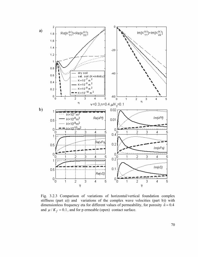
Fig. 3.2.3 Comparison of variations of horizontal/vertical foundation complex

stiffness (part a)) and variations of the complex wave velocities (part b)) with

dimensionless frequency eta for different values of permeability, for porosity ˆ 0.4n =

and / 0fK .1µ = , and for p ermeable (open) contact surface.

70

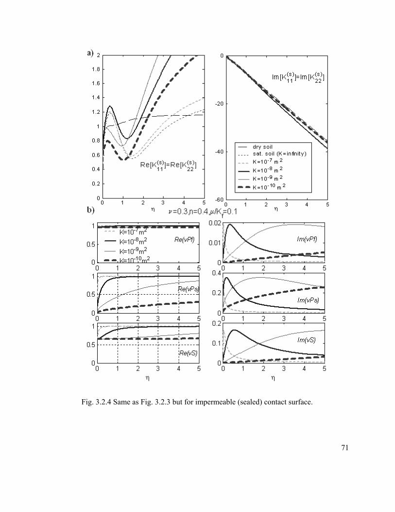
Fig. 3.2.4 Same as Fig. 3.2.3 but for impermeable (sealed) contact surface.

71

Fig. 3.2.5 Comparison of variations of horizontal/vertical foundation complex

stiffness (part a)) and variations of the complex wave velocities (part b)) with

dimensionless frequency eta for different values of permeability, for porosity ˆ 0.4n =

and / 0.fK 01µ = , and for permeable (open) contact surface.

72

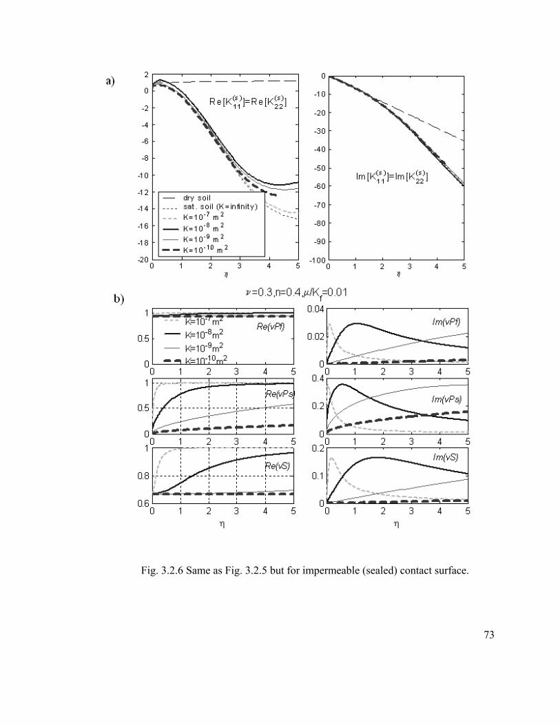
Fig. 3.2.6 Same as Fig. 3.2.5 but for impermeable (sealed) contact surface.

73

3.2.2 Foundation Complex Stiffness Matrix for Partially Saturated

Soils

Figures 3.2.7 and 3.2.8 show results for partially saturated stiff and soft soil

respectively ( / 0.1f

Kµ = and 0.01). The different curves correspond to dry soil, fully

saturated soil and partially saturated soil with saturation 99rS = % and 90%. It can be

seen that the results for the partially saturate soils are very close to those for dry soil even

for such high saturation ratios.

74

Fig. 3.2.7 Effect of degree of saturation on the foundation complex stiffness for

porosity and ˆ 0.4n = / 0.1wKµ = , and for permeable (open, part a)) and

impermeable (sealed, part b)) contact surface.

75

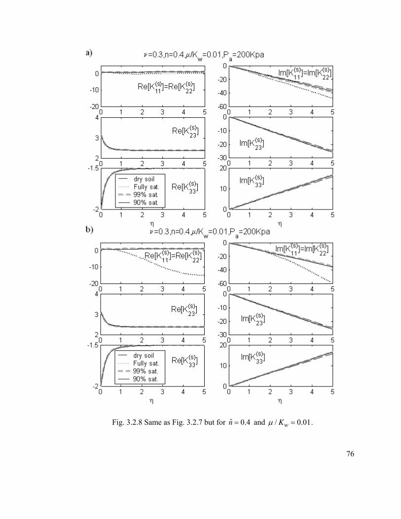
Fig. 3.2.8 Same as Fig. 3.2.7 but for ˆ 0.4n = and / 0.01wKµ = .

76

3.3 Free-Field Motion

Free-field motion is the motion of the half-space not affected by the presence of

structures. It is of interest for the problem analyzed in this thesis because it represents the

excitation of the soil-structure system. This motion is modified by the scattering of

waves from the soil-foundation interface, and radiation of waves by the vibrating

foundation. Its modification due to scattering only is referred to as foundation input

motion, which asymptotically approaches the free-field motion for wavelengths much

longer than the size of the foundation. Hence, understanding of the free-field motion

helps understand the foundation input motion. In what follows, results are shown for the

free-field motion on the surface of a porous half-space that is fully or partially saturated,

and due to incident plane fast P-wave and incident plane SV-wave. Incident slow P-wave

is not considered because it attenuates very fast, and hence is not likely to be a carrier of

any significant energy from the earthquake source. Locally generated slow P-waves,

however, are considered. The results are presented in the form of the magnitudes of the

(complex) coefficients of the reflected waves from the half-space surface, and the

magnitudes of the (complex) horizontal and vertical displacements on the surface of the

half-space. In all the results presented in this section, the Poisson’s ratio is 0.3ν = and

the porosity is . ˆ 0.4n =

77

3.3.1 Incident Plane Fast P-wave

3.3.1.1 Incident P-wave and Fully Saturated Soil

Figures 3.3.1.1 and 3.3.1.2 show variations of the reflection coefficients’ amplitudes

(left) and surface displacement amplitudes (right) due to an incident plane fast P-wave

with unit displacement amplitude, versus the angle of incidence, for different values of

permeability , and 6ˆ 10k −= 810− 1010− 2m . The case when the effects of the seepage force

are neglected is also shown, as the case , as well as the dry soil case. These two

figures differ in the stiffness of the skeleton. In Fig. 3.3.1.1

k̂ →∞

/ 0fK .1µ = (stiff soil) and

in Fig. 3.3.1.2 / 0.fK 01µ = (soft soil). Parts a) and b) differ in the hydraulic boundary

condition at the surface. Part a) corresponds to a permeable half-space and part b) to an

impermeable half-space. The frequency is set to 1f = Hz.

The results in Figs 3.3.1.1 and 3.3.1.2 show that, at 1f = Hz, the horizontal

displacements of the saturated soil decrease with decreasing permeability, are affected

very little by the type of hydraulic boundary conditions, and are always and significantly

smaller than those of the dry soil. The vertical displacements for permeable half-space

are practically not affected by the saturation for all values of permeability considered.

For impermeable half-space, vertical displacements are larger for saturated soil, and

decrease with decreasing permeability, approaching the dry soil displacements. The

difference is the largest for vertical incidence.

78

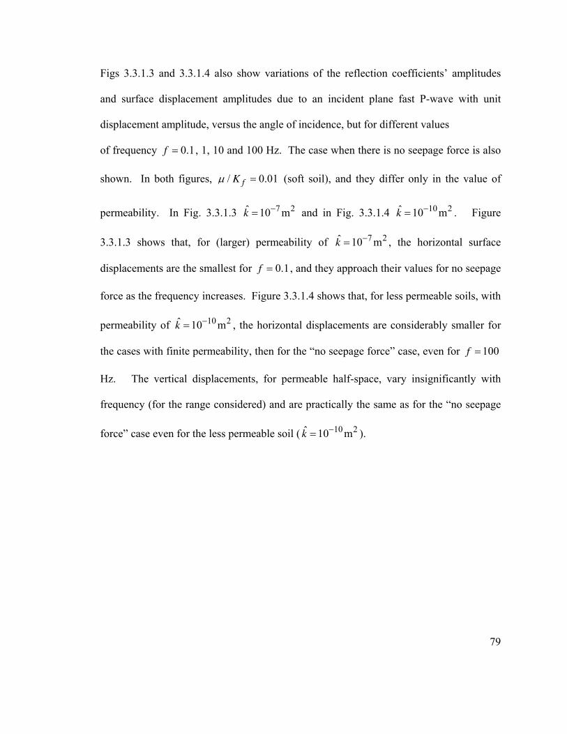
Figs 3.3.1.3 and 3.3.1.4 also show variations of the reflection coefficients’ amplitudes

and surface displacement amplitudes due to an incident plane fast P-wave with unit

displacement amplitude, versus the angle of incidence, but for different values

79

01

of frequency , 1, 10 and 100 Hz. The case when there is no seepage force is also

shown. In both figures,

0.1f =

/ 0.fKµ = (soft soil), and they differ only in the value of

permeability. In Fig. 3.3.1.3 7 2ˆ 10 mk−= and in Fig. 3.3.1.4 . Figure

3.3.1.3 shows that, for (larger) permeability of

10 2ˆ 10 mk−=

7 2ˆ 10 mk−= , the horizontal surface

displacements are the smallest for 0.1f = , and they approach their values for no seepage

force as the frequency increases. Figure 3.3.1.4 shows that, for less permeable soils, with

permeability of , the horizontal displacements are considerably smaller for

the cases with finite permeability, then for the “no seepage force” case, even for

10 2ˆ 10 mk−=

100f =

Hz. The vertical displacements, for permeable half-space, vary insignificantly with

frequency (for the range considered) and are practically the same as for the “no seepage

force” case even for the less permeable soil ( 10 2ˆ 10 mk−= ).

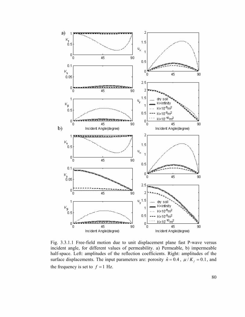
Fig. 3.3.1.1 Free-field motion due to unit displacement plane fast P-wave versus

incident angle, for different values of permeability. a) Permeable, b) impermeable

half-space. Left: amplitudes of the reflection coefficients. Right: amplitudes of the

surface displacements. The input parameters are: porosity ˆ 0.4n = , / 0.1f

Kµ = , and

the frequency is set to 1f = Hz.

80

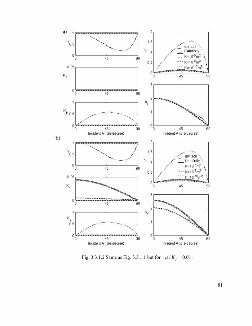
Fig. 3.3.1.2 Same as Fig. 3.3.1.1 but for / 0.01f

Kµ = .

81

Fig. 3.3.1.3 Free-field motion due to unit displacement plane fast P-wave versus

incident angle, for different values of frequency. a) Permeable, b) impermeable half-

space. The input parameters are: porosity ˆ 0.4n = , / 0.01f

Kµ = , and permeability

. 7 2ˆ 10 mk−=

82

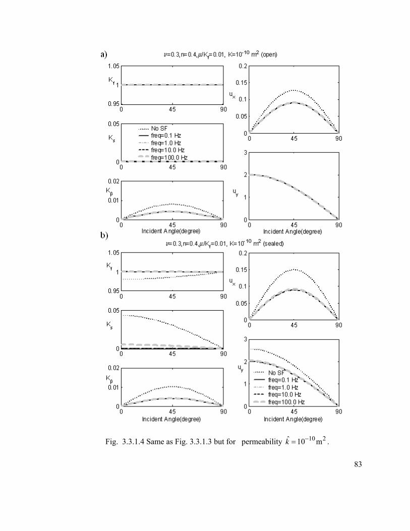
Fig. 3.3.1.4 Same as Fig. 3.3.1.3 but for permeability . 10 2ˆ 10 mk−=

83

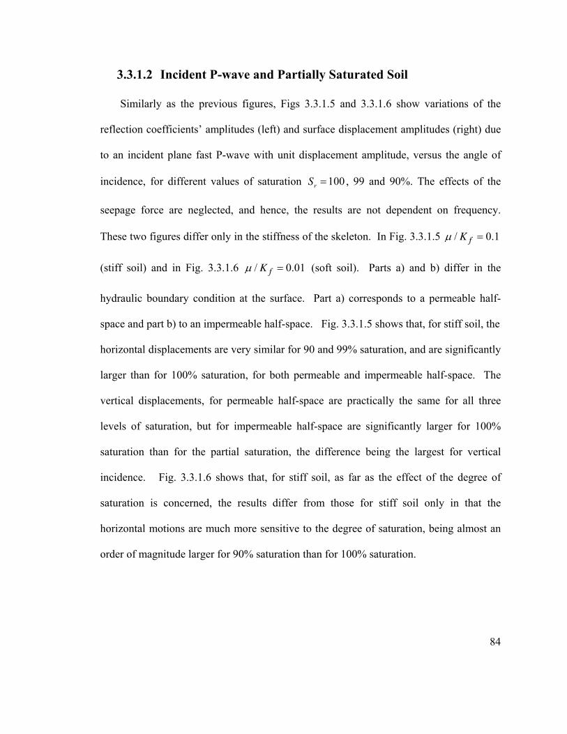
3.3.1.2 Incident P-wave and Partially Saturated Soil

Similarly as the previous figures, Figs 3.3.1.5 and 3.3.1.6 show variations of the

reflection coefficients’ amplitudes (left) and surface displacement amplitudes (right) due

to an incident plane fast P-wave with unit displacement amplitude, versus the angle of

incidence, for different values of saturation 100r

S = , 99 and 90%. The effects of the

seepage force are neglected, and hence, the results are not dependent on frequency.

These two figures differ only in the stiffness of the skeleton. In Fig. 3.3.1.5 / 0fK .1µ =

(stiff soil) and in Fig. 3.3.1.6 / 0.fK 01µ = (soft soil). Parts a) and b) differ in the

hydraulic boundary condition at the surface. Part a) corresponds to a permeable half-

space and part b) to an impermeable half-space. Fig. 3.3.1.5 shows that, for stiff soil, the

horizontal displacements are very similar for 90 and 99% saturation, and are significantly

larger than for 100% saturation, for both permeable and impermeable half-space. The

vertical displacements, for permeable half-space are practically the same for all three

levels of saturation, but for impermeable half-space are significantly larger for 100%

saturation than for the partial saturation, the difference being the largest for vertical

incidence. Fig. 3.3.1.6 shows that, for stiff soil, as far as the effect of the degree of

saturation is concerned, the results differ from those for stiff soil only in that the

horizontal motions are much more sensitive to the degree of saturation, being almost an

order of magnitude larger for 90% saturation than for 100% saturation.

84

Fig. 3.3.1.5 Free-field motion due to unit displacement plane fast P-wave versus incident

angle, for different levels of saturation. a) Permeable, b) impermeable half-space. The

input parameters are: porosity ˆ 0.4n = , / 0.1f

Kµ = , and frequency 1f = Hz. The

effects of the seepage force are neglected.

85

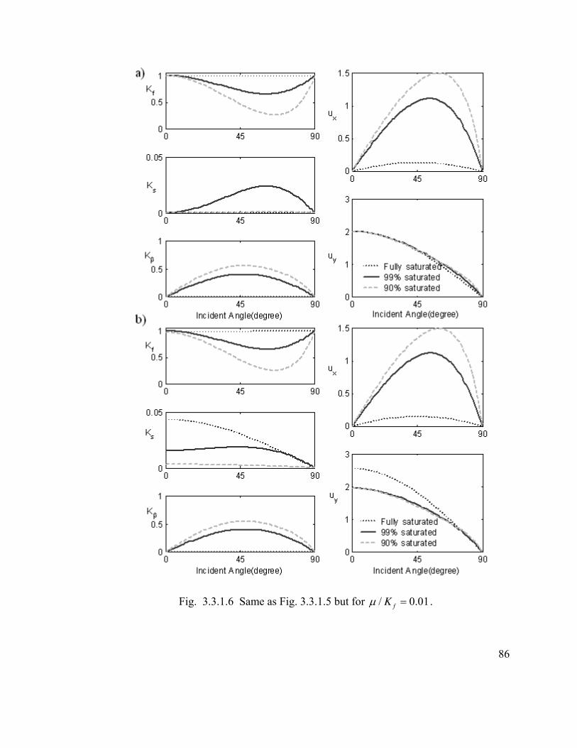
Fig. 3.3.1.6 Same as Fig. 3.3.1.5 but for / 0.01f

Kµ = .

86

3.3.2 Incident Plane SV-wave

3.3.2.1 Incident SV-wave and Fully Saturated Soil

Figures 3.3.2.1 through 3.3.2.4 show results for the free-field motion due to an

incident plane SV-wave onto a half-space for the same parameters as Figs 3.3.1.1 through

3.3.1.4. It can be seen that for vertical incidence, the horizontal displacement on the

surface always approaches 2, and the vertical displacement approaches zero. As the

incident angle approaches 90 , both the vertical and horizontal displacements approach

zero. For incidence, and for permeable half-space, the horizontal displacements are

always zero, while for impermeable half-space, they are not necessarily zero but are

small. It can be seen that the surface displacements for incident SV wave are not very

sensitive to the hydraulic boundary condition. A comparison with the results for incident

P-wave shows that, for incident SV-wave, both the horizontal and vertical surface

displacements are more sensitive to the variations of permeability and frequency, i.e. are

affected more by the seepage force, than for incident P-wave. For frequency set to

45

1f =

Hz, the maximum displacement amplitudes (over all incident angles) are significantly

larger for larger seepage force than for “no seepage force” (see Figs 3.3.2.1 and 3.3.2.2),

but as the frequency increases, they decrease and approach the values for “no seepage

force”. A comparison of the fully saturated and dry soil cases shows that the maximum

horizontal displacements (over all incident angles) are larger for the dry soil, while the

vertical displacements are larger for the saturated soil, and for smaller permeability.

87

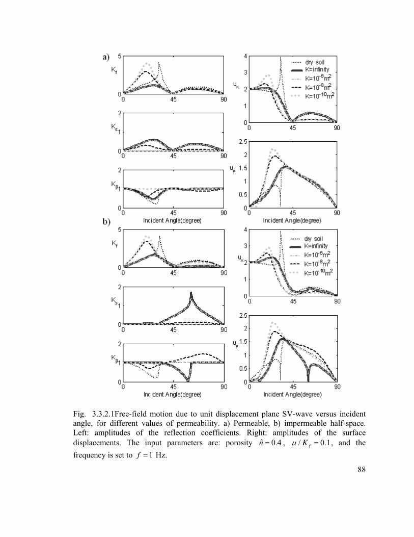
Fig. 3.3.2.1Free-field motion due to unit displacement plane SV-wave versus incident

angle, for different values of permeability. a) Permeable, b) impermeable half-space.

Left: amplitudes of the reflection coefficients. Right: amplitudes of the surface

displacements. The input parameters are: porosity ˆ 0.4n = , / 0.1f

Kµ = , and the

frequency is set to 1f = Hz.

88

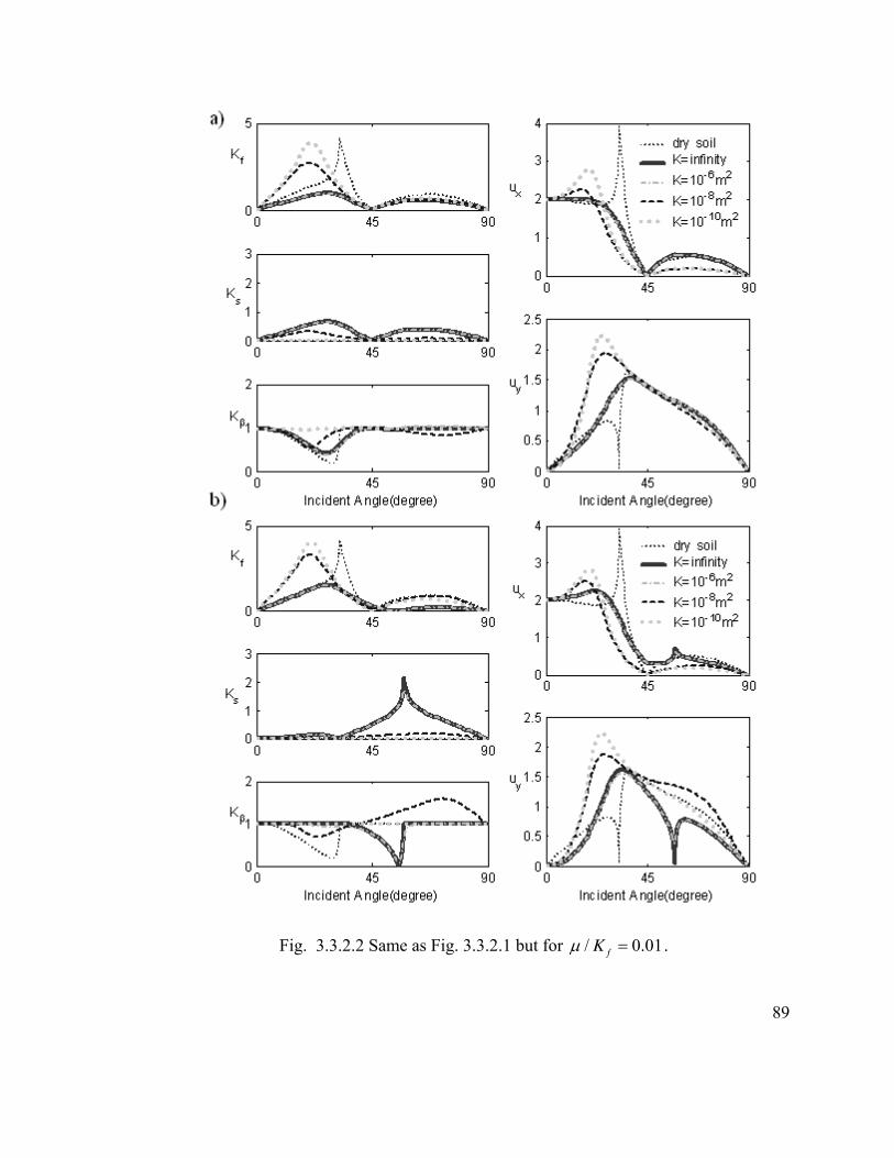
Fig. 3.3.2.2 Same as Fig. 3.3.2.1 but for / 0.01f

Kµ = .

89

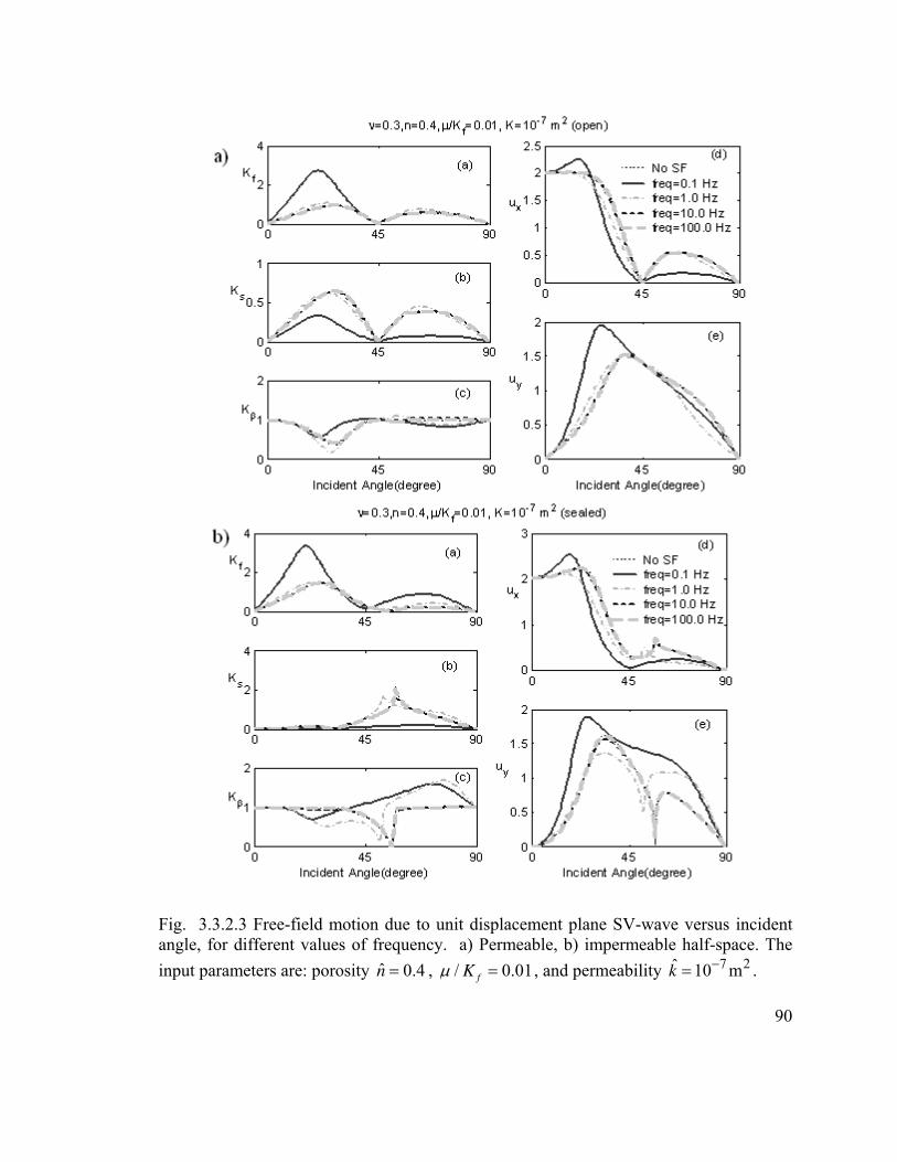
Fig. 3.3.2.3 Free-field motion due to unit displacement plane SV-wave versus incident

angle, for different values of frequency. a) Permeable, b) impermeable half-space. The

input parameters are: porosity ˆ 0.4n = , / 0.01f

Kµ = , and permeability . 7 2ˆ 10 mk−=

90

Fig. 3.3.2.4 Same as Fig. 3.3.2.3 but for permeability . 10 2ˆ 10 mk−=

91

92

3.3.2.2 Incident SV-wave and Partially Saturated Soil

Figs 3.3.2.5 and 3.3.2.6 show results for the free-field motion due to an incident SV-

wave for partial saturation, also for the same soil properties as in Figs 3.3.1.5 and 3.3.1.6.

It can be seen from these results that the vertical displacements are not very sensitive to

the degree of saturation, but the maximum (over all incident angles) horizontal

amplitudes are much larger for the partially saturated soils than for the fully saturated

soil.

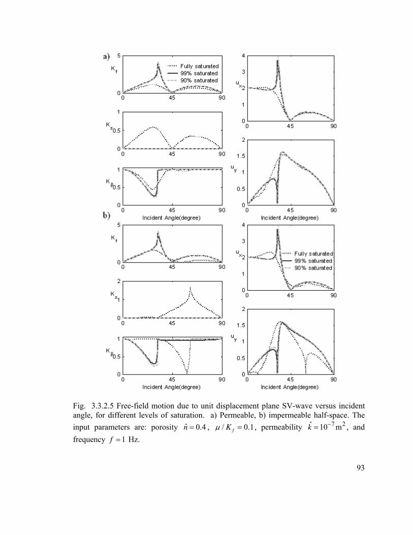
Fig. 3.3.2.5 Free-field motion due to unit displacement plane SV-wave versus incident

angle, for different levels of saturation. a) Permeable, b) impermeable half-space. The

input parameters are: porosity ˆ 0.4n = , / 0.1f

Kµ = , permeability , and

frequency

7 2ˆ 10 mk−=

1f = Hz.

93

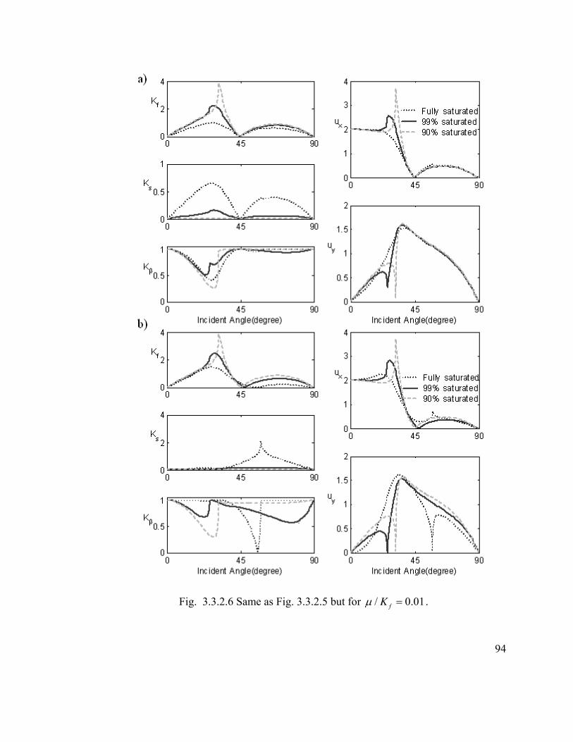
Fig. 3.3.2.6 Same as Fig. 3.3.2.5 but for / 0.01f

Kµ = .

94

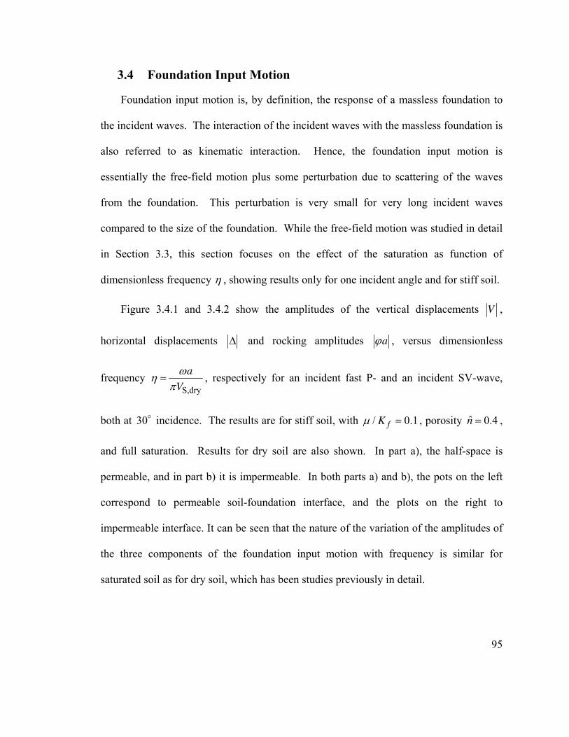
3.4 Foundation Input Motion

Foundation input motion is, by definition, the response of a massless foundation to

the incident waves. The interaction of the incident waves with the massless foundation is

also referred to as kinematic interaction. Hence, the foundation input motion is

essentially the free-field motion plus some perturbation due to scattering of the waves

from the foundation. This perturbation is very small for very long incident waves

compared to the size of the foundation. While the free-field motion was studied in detail

in Section 3.3, this section focuses on the effect of the saturation as function of

dimensionless frequency η , showing results only for one incident angle and for stiff soil.

Figure 3.4.1 and 3.4.2 show the amplitudes of the vertical displacements V ,

horizontal displacements ∆ and rocking amplitudes aϕ , versus dimensionless

frequency S,dry

a

V

ωηπ

= , respectively for an incident fast P- and an incident SV-wave,

both at 30 incidence. The results are for stiff soil, with / 0fK .1µ = , porosity ˆ 0.4n = ,

and full saturation. Results for dry soil are also shown. In part a), the half-space is

permeable, and in part b) it is impermeable. In both parts a) and b), the pots on the left

correspond to permeable soil-foundation interface, and the plots on the right to

impermeable interface. It can be seen that the nature of the variation of the amplitudes of

the three components of the foundation input motion with frequency is similar for

saturated soil as for dry soil, which has been studies previously in detail.

95

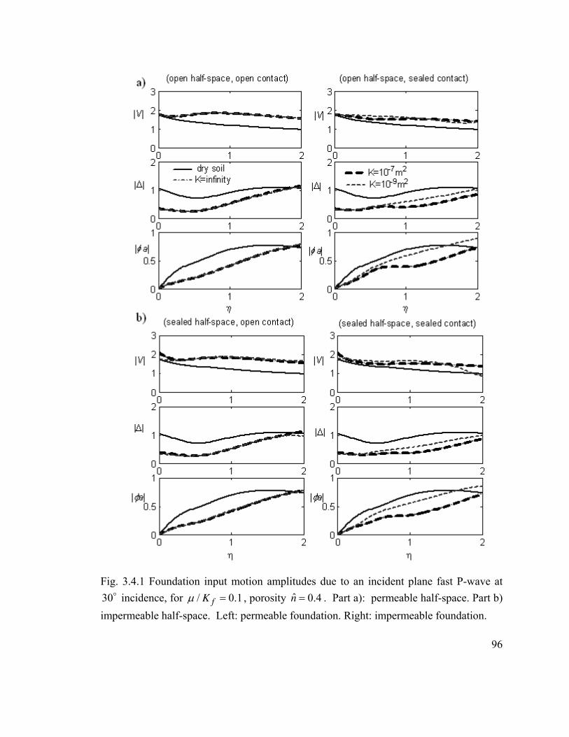
Fig. 3.4.1 Foundation input motion amplitudes due to an incident plane fast P-wave at

incidence, for 30 / 0fK .1µ = , porosity ˆ 0.4n = . Part a): permeable half-space. Part b)

impermeable half-space. Left: permeable foundation. Right: impermeable foundation.

96

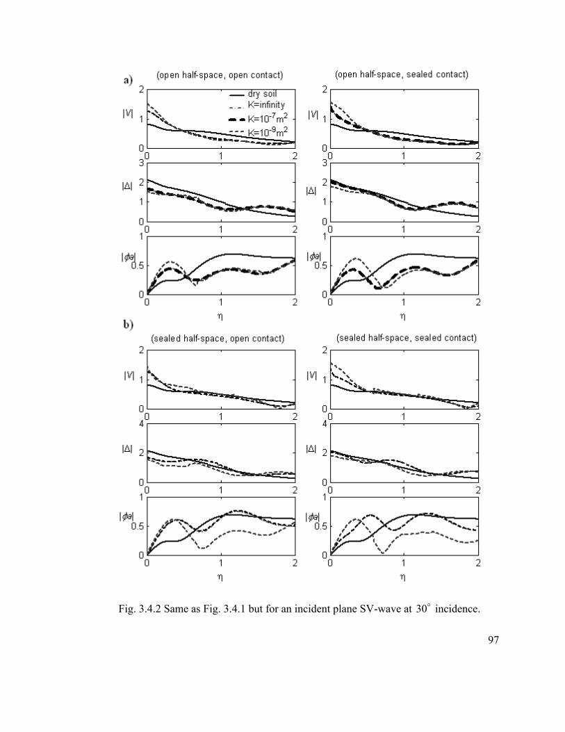
Fig. 3.4.2 Same as Fig. 3.4.1 but for an incident plane SV-wave at incidence. 30

97

3.5 Building-Foundation-Soil Response

98

.1

This section shows results for the amplitudes of the foundation displacements and

building relative displacement (due to elastic deformation of the building only), for stiff

soil with / 0fKµ = and porosity ˆ 0.4n = , and for a building with height 2H a= ,

width , and mass ratios W a= / 2b f

m m = and / 0.2f s

m m = . The excitation is an

incident plane fast P-wave or a plane SV-wave, both at incidence, and with unit

displacement of the incident wave.

30

3.5.1 Building-Foundation-Soil Response for Incident P-wave

Figures 3.5.1.1 through 3.5.1.4 show results for incident P-wave at 30 incidence. In

all figures, V is the amplitudes of the vertical displacements, ∆ is the amplitudes of the

horizontal displacements, aϕ is the rocking angle multiplied by the characteristic length

a, relbu is the relative building response at the top, and the dimensionless frequency is

S,dry

a

V

ωηπ

= . In each figure, part a) corresponds to permeable half-space, and part b) to

impermeable half-space.

Figures 3.5.1.1 and 3.5.1.2 show the variation of the system response with η for fully

saturated soil with different permeability, respectively for permeable and for

impermeable foundation. The response for dry soil is also shown. Figures 3.5.1.3 and

3.5.1.4 show the variation of the system response with η for different levels of

saturation. These figures show that both the foundation and the building relative

response exhibit large variations near the building fixed-base frequencies. The

99

“backbone” curve of the foundation displacement amplitudes is governed by the

foundation input motion, shown in Section 3.4, which also affects the amplitudes of the

peaks of the building relative response. The building relative response has peaks at the

system frequencies. Due to the interaction with the foil, the first system frequency is

lower than the fundamental fixed-base frequency, and the amplitude of the peak is

generally reduced due to the radiation of energy in the soil. It is well known that the

amount of the shift and the reduction of amplitude depend on the relative flexibility of the

soil, which in case of porous soil depends on the water content, soil permeability, and

also frequency. The effect of the flexibility of the soil is described through the

foundation complex stiffness matrix (See Section 3.2). In the “coarse” resolution plots in

these figures, no significant shift of the peaks can be seen as function of the water content

and permeability. Hence, if there is a change, it is small. Investigation of such changes

for one case study building is presented in the following section.

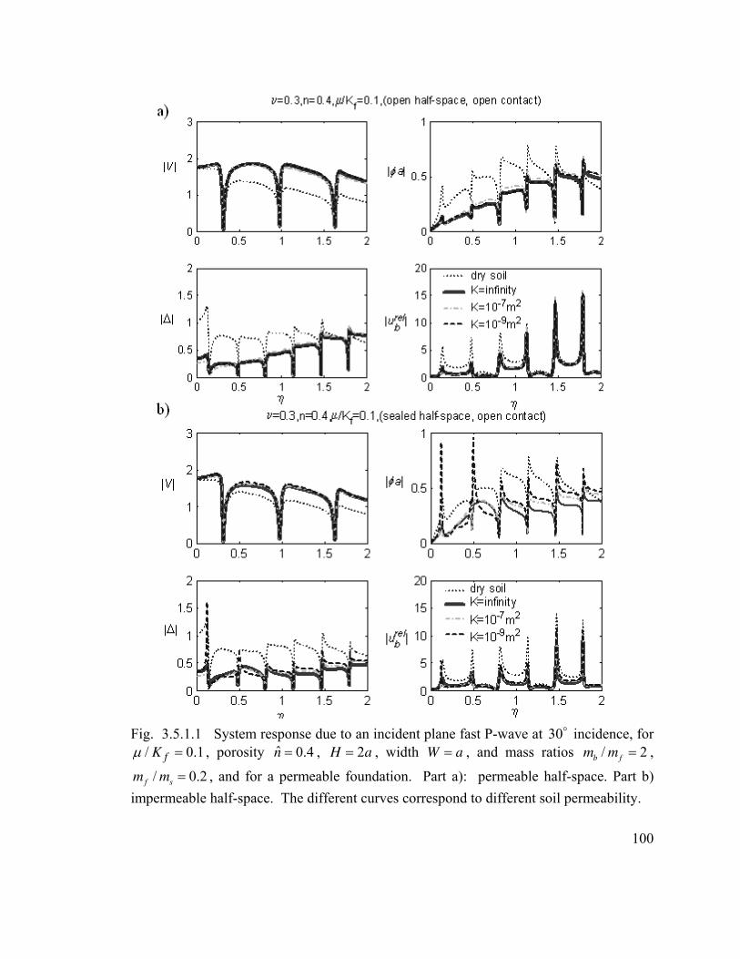
Fig. 3.5.1.1 System response due to an incident plane fast P-wave at 30 incidence, for

/ 0fK .1µ = , porosity , ˆ 0.4n = 2H a= , width W a= , and mass ratios / 2b f

m m = ,

, and for a permeable foundation. Part a): permeable half-space. Part b)

impermeable half-space. The different curves correspond to different soil permeability.

/ 0f s

m m = .2

100

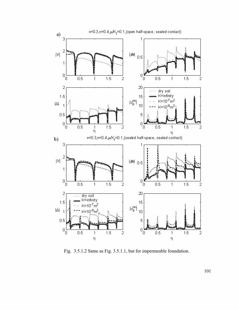
Fig. 3.5.1.2 Same as Fig. 3.5.1.1, but for impermeable foundation.

101

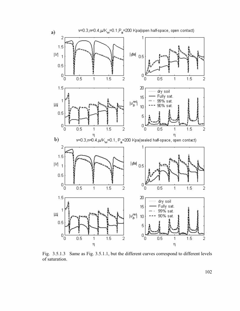
Fig. 3.5.1.3 Same as Fig. 3.5.1.1, but the different curves correspond to different levels

of saturation.

102

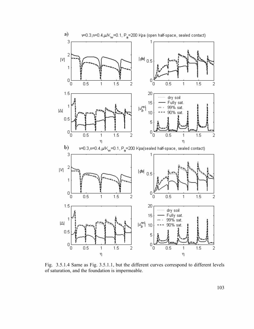
Fig. 3.5.1.4 Same as Fig. 3.5.1.1, but the different curves correspond to different levels

of saturation, and the foundation is impermeable.

103

3.5.2 Building-Foundation-Soil Response for Incident SV-wave

Similarly as in Section 3.5.1, Figures 3.5.2.1 through 3.5.2.4 show results for

incident SV-wave at 30 incidence. In all figures, V is the amplitudes of the vertical

displacements, ∆ is the amplitudes of the horizontal displacements, aϕ is the rocking

angle multiplied by the characteristic length a, relbu is the relative building response at

the top, and the dimensionless frequency is S,dry

a

V

ωηπ

= . In each figure, part a)

corresponds to permeable half-space, and part b) to impermeable half-space. The

observations in these figures are the same as in Section 3.5.1 for incident P-wave.

104

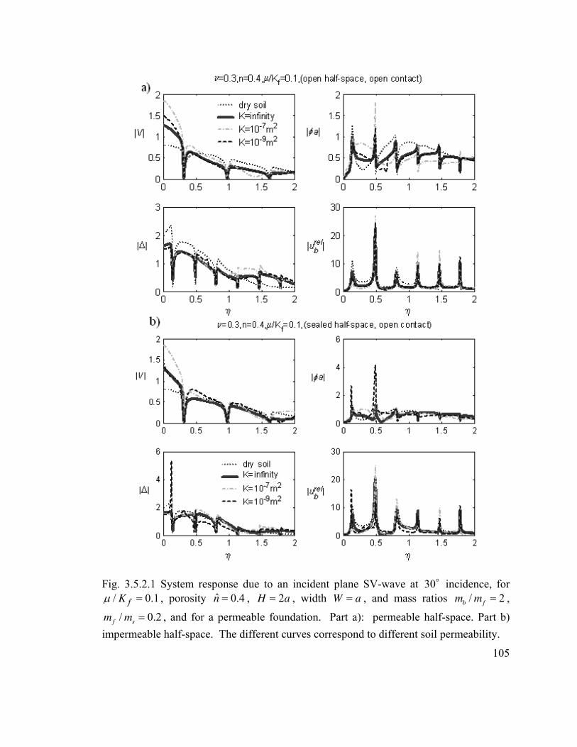
Fig. 3.5.2.1 System response due to an incident plane SV-wave at 30 incidence, for

/ 0fK .1µ = , porosity , ˆ 0.4n = 2H a= , width W a= , and mass ratios / 2b f

m m = ,

, and for a permeable foundation. Part a): permeable half-space. Part b)

impermeable half-space. The different curves correspond to different soil permeability.

/ 0f s

m m = .2

105

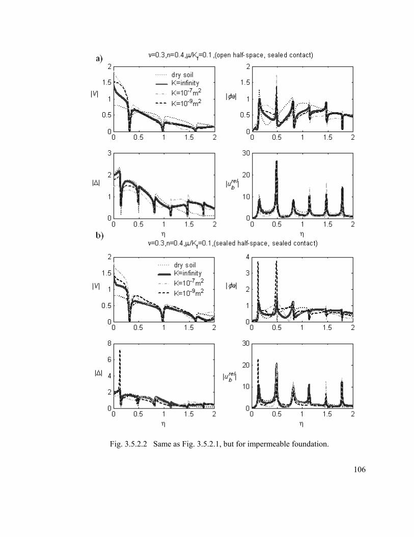
Fig. 3.5.2.2 Same as Fig. 3.5.2.1, but for impermeable foundation.

106

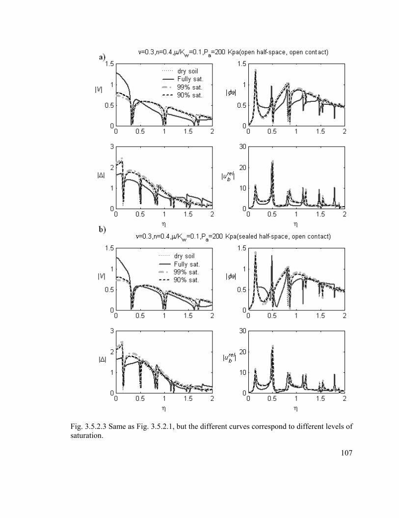
Fig. 3.5.2.3 Same as Fig. 3.5.2.1, but the different curves correspond to different levels of

saturation.

107

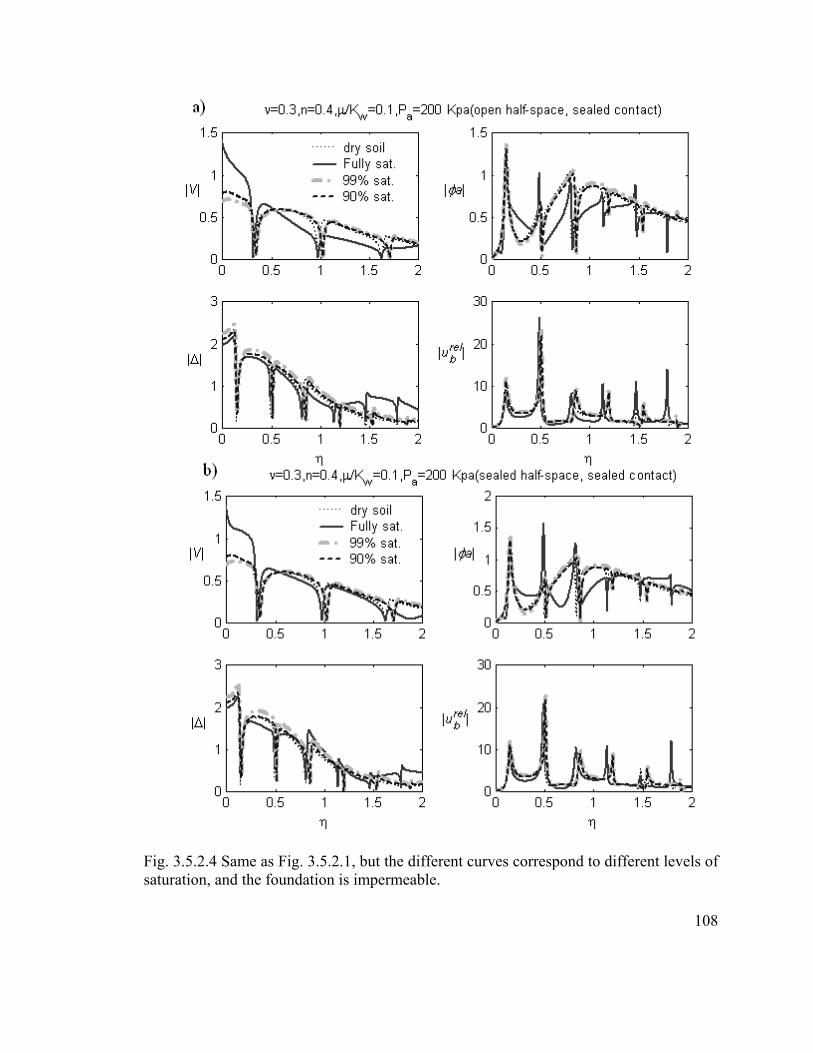
Fig. 3.5.2.4 Same as Fig. 3.5.2.1, but the different curves correspond to different levels of

saturation, and the foundation is impermeable.

108

109

3.6 Frequency Shift due to Saturation – Millikan Library Case

This section shows results for the model response for parameters chosen so that it

corresponds approximately to the NS response of Millikan Library in Pasadena,

California. This building has been chosen because changes of its frequencies of vibration

have been reported such that can be correlated with heavy rainfall (Clinton et al., 2006).

Todorovska and Al Rjoub (2006b) attempted to explain these changes as resulting from

changes in the soil due to saturation. They used a soil-structure interaction model in

poroelastic soils, presented in Todorovska and Al Rjoub (2006a), and showed that

changes in the soil due to saturation produced the same trend and order of magnitude of

the shift as observed. The model of Todorovska and Al Rjoub (2006a) is an earlier

version of the model analyzed in this thesis that did not include the effects of the seepage

force. Hence, this section focuses on how different assumptions on the soil permeability

would affect the frequency shift. For the purpose of completeness of the analysis in this

thesis work, a summary of the full-scale observations, as well as of the choice of model

parameters in Todorovska and Al Rjoub (2006b) is included.

3.6.1 Full-scale Observations

The frequencies of vibration of Millikan Library have been monitored since 1967

using different excitations such as ambient noise, forced vibrations, and earthquakes.

Permanent and temporary changes in its frequencies have been observed, most recently

summarized in Clinton et al. (2006). The permanent change is decrease with time, from

1.45 to 1.19 Hz for EW vibrations, and from 1.9 to 1.72 Hz for NS vibrations, as

measured during small amplitude vibrations. The lowest measured values occurred

110

during the strong earthquake shaking from the 1971 San Fernando earthquake (Udwadia

and Trifunac, 1974), and 1994 Northridge earthquake (0.94 Hz for EW vibrations, and

1.33 Hz for NS vibrations; Cinton et al., 2006). Since February of 2001, continuous data

steams of the 9th

floor response have been recorded by a tri-axial 24-bit accelerometer,

which is one of the stations of the California Integrated Seismic Network. This has

enabled monitoring of changes of the building apparent frequencies on different time

scales (Clinton et al., 2006). Further, weather data from the nearby JPL Weather station,

located about 8.5 km north of the building, has been available for a period of about 2.5

years following the installation of this sensor, which enabled to study possible

correlations of the changes of its frequencies with weather (temperature, wind and rain).

The reported observation of the changes of the building frequencies with rainfall is

as follows. The building first and second apparent frequencies for EW and NS motions,

and the first frequency for torsional motions increase during heavy rainfall (above 40 mm

per day) in a matter of hours, and recover in about a week following the rain (Clinton,

2004; Clinton et al., 2006). For example, in early February of 2003, when over 100 mm

rain fell over a period of two days, an increase of about 3% was measured for the EW and

the torsional frequencies, followed by a slow decay over a period of about 10 days (see

Fig. 9 in Clinton et al., 2006). The measured change of the NS frequency was smaller

(slightly less than 1%). Clinton et al. (2006) note that this increase in frequencies

occurred in spite of the fact that strong winds that often accompany heavy rainfall tend to

decrease the system frequencies by exciting larger amplitudes of response (by up to 3%

in dry weather). Further, they note an increase of the system frequencies with

temperature (about 1−2 % on very hot days with temperature near 40oC). For wind and

temperature, the recovery is practically instantaneous, while for rainfall it is slow, and

can take about a week.

3.6.2 Model Parameters for NS Response

Todorovska and Al Rjoub (2006b) chose the system parameters guided by the

information provided in Luco et al. (1986), who specified: building weight =

N, foundation weight = N, building height 44 m, foundation depth 4 m, and

building in plan dimensions

81.05 10×

80.14 10×

21 m 23 m× . Further, they classify the local soil as alluvium

with depth to “bedrock” about 275 m, and mention apparent frequencies of vibration

measured during forced vibration tests that are about 1 1.8f = Hz for NS vibrations, and

Hz for EW vibrations. Clinton et al. (2005) provided further history on the

variations of these frequencies, which shows strong correlation with amplitudes of

response, and overall trend of decrease with time, from initial values Hz for NS

vibrations, and Hz for EW vibrations during forced vibrations in 1967, to

Hz for NS vibrations, and

1 1.4f =

1 1.9f =

1 1.45f =

1 1.54f = 1 1.19f = Hz for EW vibrations during ambient

vibrations. For the soil in their homogeneous half-space model, Todorovska and Al

Rjoub (2006b) chose values that would correspond approximately to the soil at Millikan

Library near the surface. They use soil porosity = 0.4, Poisson’s ratio n̂ sν = 0.3,

kg/m3gr 2.7 10ρ = × 3

, and sµ that correspond to dry shear wave velocity

,dry grˆ/[(1 ) ]S sV nµ ρ= − = 300 m/s. For the water, kg/m310fρ = 3 and 92.2 10fK = ×

111

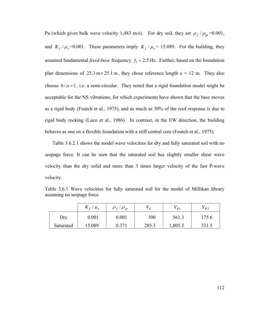
Pa (which gives bulk wave velocity 1,483 m/s). For dry soil, they set gr/fρ ρ =0.001,

and /fK sµ =0.001. These parameters imply /fK sµ = 15.089. For the building, they

assumed fundamental fixed-base frequency 1 2.5f = Hz. Further, based on the foundation

plan dimensions of , they chose reference length a = 12 m. They also

choose , i.e. a semi-circular. They noted that a rigid foundation model might be

acceptable for the NS vibrations, for which experiments have shown that the base moves

as a rigid body (Foutch et al., 1975), and as much as 30% of the roof response is due to

rigid body rocking (Luco et al., 1986). In contrast, in the EW direction, the building

behaves as one on a flexible foundation with a stiff central core (Foutch et al., 1975).

23.3 m 25.1 m×

/b a =1

Table 3.6.2.1 shows the model wave velocities for dry and fully saturated soil with no

seepage force. It can be seen that the saturated soil has slightly smaller shear wave

velocity than the dry solid and more than 3 times larger velocity of the fast P-wave

velocity.

Table 3.6.1 Wave velocities for fully saturated soil for the model of Millikan library

assuming no seepage force

/f sK µ /f grρ ρ SV 1PV 2PV

Dry 0.001 0.001 300 561.3 175.6

Saturated 15.089 0.371 285.3 1,805.3 331.5

112

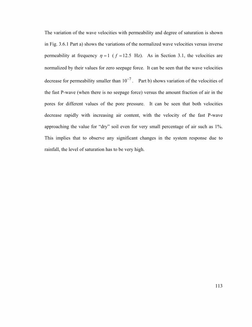
The variation of the wave velocities with permeability and degree of saturation is shown

in Fig. 3.6.1 Part a) shows the variations of the normalized wave velocities versus inverse

permeability at frequency 1η = ( 12.5f = Hz). As in Section 3.1, the velocities are

normalized by their values for zero seepage force. It can be seen that the wave velocities

decrease for permeability smaller than 710− . Part b) shows variation of the velocities of

the fast P-wave (when there is no seepage force) versus the amount fraction of air in the

pores for different values of the pore pressure. It can be seen that both velocities

decrease rapidly with increasing air content, with the velocity of the fast P-wave

approaching the value for “dry” soil even for very small percentage of air such as 1%.

This implies that to observe any significant changes in the system response due to

rainfall, the level of saturation has to be very high.

113

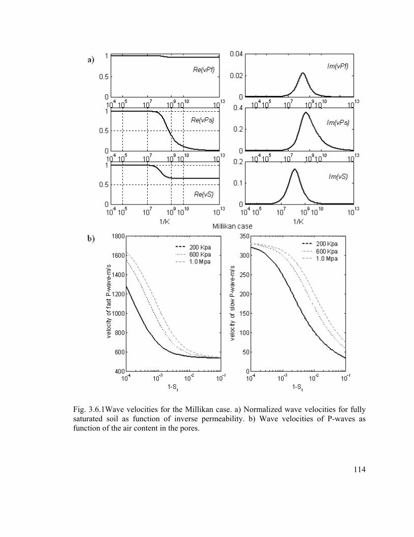
Fig. 3.6.1Wave velocities for the Millikan case. a) Normalized wave velocities for fully

saturated soil as function of inverse permeability. b) Wave velocities of P-waves as

function of the air content in the pores.

114

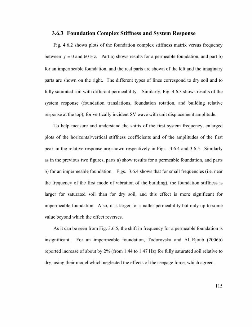
3.6.3 Foundation Complex Stiffness and System Response

Fig. 4.6.2 shows plots of the foundation complex stiffness matrix versus frequency

between 0 and 60 Hz. Part a) shows results for a permeable foundation, and part b)

for an impermeable foundation, and the real parts are shown of the left and the imaginary

parts are shown on the right. The different types of lines correspond to dry soil and to

fully saturated soil with different permeability. Similarly, Fig. 4.6.3 shows results of the

system response (foundation translations, foundation rotation, and building relative

response at the top), for vertically incident SV wave with unit displacement amplitude.

f =

To help measure and understand the shifts of the first system frequency, enlarged

plots of the horizontal/vertical stiffness coefficients and of the amplitudes of the first

peak in the relative response are shown respectively in Figs. 3.6.4 and 3.6.5. Similarly

as in the previous two figures, parts a) show results for a permeable foundation, and parts

b) for an impermeable foundation. Figs. 3.6.4 shows that for small frequencies (i.e. near

the frequency of the first mode of vibration of the building), the foundation stiffness is

larger for saturated soil than for dry soil, and this effect is more significant for

impermeable foundation. Also, it is larger for smaller permeability but only up to some

value beyond which the effect reverses.

As it can be seen from Fig. 3.6.5, the shift in frequency for a permeable foundation is

insignificant. For an impermeable foundation, Todorovska and Al Rjoub (2006b)

reported increase of about by 2% (from 1.44 to 1.47 Hz) for fully saturated soil relative to

dry, using their model which neglected the effects of the seepage force, which agreed

115

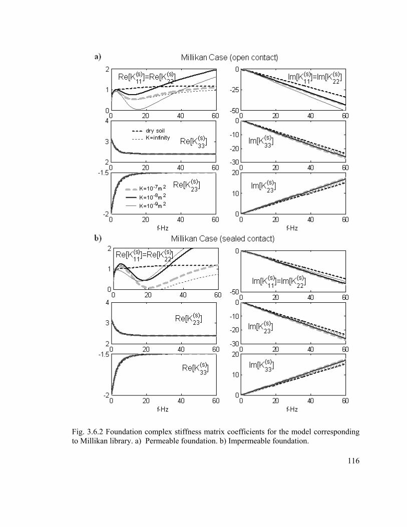
Fig. 3.6.2 Foundation complex stiffness matrix coefficients for the model corresponding

to Millikan library. a) Permeable foundation. b) Impermeable foundation.

116

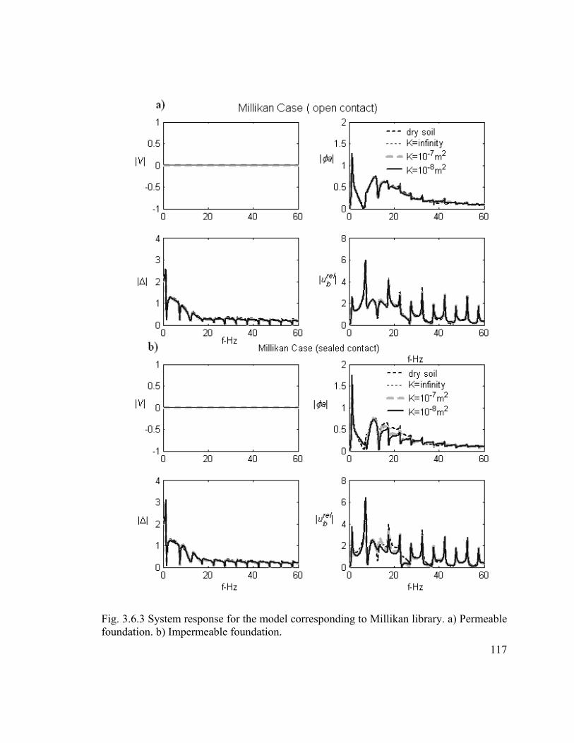
Fig. 3.6.3 System response for the model corresponding to Millikan library. a) Permeable

foundation. b) Impermeable foundation.

117

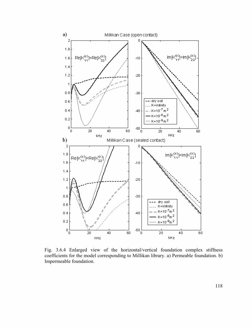
Fig. 3.6.4 Enlarged view of the horizontal/vertical foundation complex stiffness

coefficients for the model corresponding to Millikan library. a) Permeable foundation. b)

Impermeable foundation.

118

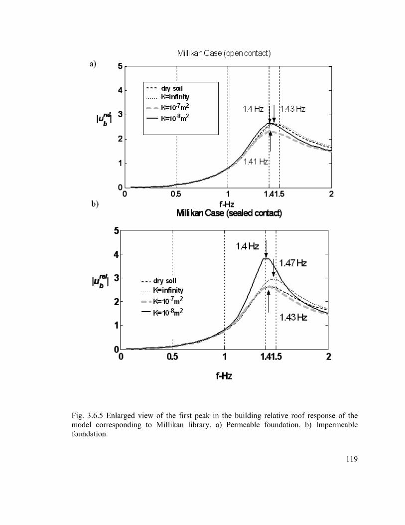
Fig. 3.6.5 Enlarged view of the first peak in the building relative roof response of the

model corresponding to Millikan library. a) Permeable foundation. b) Impermeable

foundation.

119

approximately with the observations. Fig. 3.6.5 (part b)) shows that this effect is smaller

for less permeable soils and may reverse for small enough permeability of the soil.

It is noted here that the observed effect of finite permeability on the shift of frequency

predicted by the model is due to the strong dependency of the wave velocities in Biot’s

original theory (Biot, 1956a) on permeability and frequency, i.e. for large enough ˆ ˆ1

ˆ

n

k

µω

.

This dependency is most significant for the shear wave velocity, which can be reduces to

up to 60-70% of its value for zero seepage force. This reduction is due to increased

effective mass (due to the seepage force) in the computation of the wave velocities. It is

also noted that Biot’s theory does not consider the molecular forces between the different

phases (solid, water and air in the case of partial saturation).

120

121

Chapter 4: Summary and Conclusions

This thesis presented an investigation of the effects of water saturation on the

effective input motion and system response during building-foundation-soil interaction

using a simple two-dimensional model. In this model, the building is represented as a

shear wall supported by a semi-cylindrical foundation imbedded in a homogeneous and

isotropic poroelastic half-space, and the excitation is a plane P, plane SV or a Rayleigh

wave. Biot’s theory of wave propagation in fully saturated poroelastic medium was used

to describe the motion in the soil. By relaxing the zero stress condition at the free surface

for the scattered waves, a closed form solution was derived using the wave function

expansion method. The boundary conditions along the contact surface between the soil

and the foundation are perfect bond for the skeleton, and either drained or undrained

hydraulic condition for the fluid (i.e. permeable or impermeable boundary). The effect of

partial saturation, versus full saturation for which the Biot’s theory has been derived, is

accounted for approximately, by changing the effective bulk modulus of the fluid.

Numerical results are shown for variations of the wave velocities, free-field motion

amplitudes, foundation input motion amplitudes, foundation complex stiffness, and the

system response in the frequency domain for different values of the model parameters,

and for incident plane P- and SV-waves. Also, the effects of the saturation on the

building apparent frequency are analyzed for a model that approximately corresponds to

the NS response Millikan library in Pasadena, California, for which shift in frequency

and recovery have been observed due to heavy rainfall. The numerical results were

computed using a computer program written in Fortran. The following summarizes the

results of the analysis and the conclusions.

The solution of the problem was expressed entirely in terms of dimensionless

parameters, which were defined using reference: length (half with of the foundation),

material modulus

a

sµ (the shear modulus of the skeleton), and mass density grρ (the

density of the material of the grains without pores). The dimensionless parameters that

control the system response are the following: stiffness of the skeleton relative to the bulk

modulus of the fluid, through the ratio /s fKµ and the Poisson’s ratio sν ; mass density

of the skeleton relative to the fluid, defined through the ratio gr / fρ ρ and the porosity ;

mass of the building relative to the mass of the foundation, and mass of the foundation

relative to the mass of the replaced soil, through the ratios

n̂

b fnd/m m and ,

where,

fnd gr/m m

gr fnd grm A ρ= is the mass of the excavated soil (per unit length) if there were no

voids, and is the area of the foundation; the flexibility of the building relative to that

of the soil, through the ratio

fndA

ref ,b( ) /( ) [ ],b ref( ) / / ( ) /SH V a Vω ω⎡ ⎤= ⎣ ⎦SV H V aε = = ratio of

the number of wavelength in the shear beam in length H and the number of reference

wavelengths in the soil in length a; dimensionless frequency ref/( )a Vη ω π= , where

ref gr/sV µ ρ= is a reference velocity; foundation shape, through the ratio ; and on

the type, amplitude and angle of the incident waves. An additional parameter for viscous

fluids and finite permeability is the coefficient of dissipation

/h a

2ˆ ˆˆ ˆ /b n kµ= , were µ̂ is the

absolute viscosity, and is the coefficient of permeability. k̂

122

The wave velocities in the soil medium are the most fundamental quantities that

affect the system response. Therefore, the effects of the model parameters on the wave

velocities were first analyzed. Biot’s theory predicts the existence of two P-waves (one

fast and the other one slow) and one S-wave in poroelastic soil medium. The results

show that, when the seepage force is considered, the velocities of these waves are

frequency dependent. The wave velocities in the soil decrease with increasing seepage

force, the effects of which are more pronounced for smaller frequency of motion, larger

fluid viscosity, larger porosity and smaller skeleton permeability, i.e. for larger ˆ ˆ1

ˆ

n

k

µω

.

For large enough ˆ ˆ1

ˆ

n

k

µω

, the velocities of the SV and fast P-wave approach their

asymptotic value, which is real valued, and the velocity of the slow P-wave approaches

zero. The variation is very small for the fast P-waves (about 5%), is about up to 40% for

the S-wave, and is up to 100% for the slow P-wave. The percentage change depends very

little on the relative stiffness of the skeleton (i.e. /s fKµ ). Both P-wave velocities

decrease with increasing air content in the pores. The velocity of the fast P-wave

approaches the P-wave velocity of the dry soil, and that of the slow P-wave approaches

zero.

The results show that the amplitudes of the free-field motion, which excites the

structure, depend strongly on the angle of incidence, and also on the properties of the soil

model: relative stiffness of the skeleton (i.e. /s fKµ ), porosity and permeability (for

given viscosity and Poisson’s ratio), and are frequency dependent when ˆ ˆ1

ˆ

n

k

µω

is not

123

small. The effect of the water is more significant for mixtures with softer skeleton (i.e.

smaller /s fKµ ), e.g. soft soils, as compared to porous rock. For incident P-wave, the

amplitudes of the horizontal motion at the surface are larger for dry soil than for saturated

soil, but the amplitudes of the vertical motion are larger for saturated soil and

impermeable boundary. For incident SV wave, the peak horizontal amplitude is also

larger for dry soil, and but the vertical amplitudes are smaller regardless of the hydraulic

boundary condition on the surface.

The amplitudes of the free-field displacements at the ground surface depend most on

the incident angle. For incident P waves, the amplitude of the horizontal displacement is

zero for vertically and horizontally incident waves, and is the largest near 45 degrees

incidence. The amplitudes of the vertical displacement is the maximum for vertical

incidence, and it decreases monotonically to zero for horizontal incidence. For incident

SV waves and Poison ratio ν =0.3, the horizontal amplitude equals 2 for vertical

incidence, is zero at 45 degrees incidence, exhibiting a sharp peak for incidence below 45

degrees, beyond which it increases a little and decreases again to zero for horizontal

incidence. The amplitudes for the vertical motion are zero for vertical and horizontal

incidence, and exhibit a peak near 30 degrees incidence. The frequency dependence is

more significant for incident SV waves, but it is still small. The amplitudes decrease

with increasing frequency, approaching those for zero seepage force.

The foundation input motion is the effective input motion exciting the structure. It is

defined as the response of a massless foundation, without the structure, to the incident

waves, and represents the free field motion that has been modified by the scattering of

124

waves from the foundation. As the dimensionless frequency 0η → (i.e. for very long

incident waves compared to the size of the foundation), the horizontal and vertical

amplitudes of the foundation input motion approach those of the free-field motion, and

the rotation approaches zero. For very short incident wavelengths, the amplitudes

approach zero, due to the ironing effect of the foundation.

The building response is affected by the dynamic soil-structure interaction through

the foundation complex stiffness matrix. The real part of this matrix is referred to as

“foundation stiffness”, and the imaginary part is related to the loss of energy due to

radiation which effect is related to the “radiation damping”. The results show that the

presence of water in the pores affects significantly the foundation impedance matrix for

soft and stiff soils. The rocking impedance is affected negligibly by the presence of

water, which can be explained by the fact that the rocking motions produce mostly a

shearing deformation of the soil near the contact surface. The conclusion is similar for

the coupling term. The horizontal impedance is significantly affected by the hydraulic

condition along the contact surface, which permits or stops the flow of water through the

contact surface. As it can be expected, the foundation stiffness is larger when the pores

are filled with water and the contact surface is impermeable (sealed contact). The

imaginary part, however, i.e. the radiation damping, is larger for permeable foundation.

For relatively small seepage force, the foundation stiffness increases with increasing

seepage force, but for large enough seepage force the effect becomes the opposite. In

that case, the decreasing foundation stiffness with increasing seepage force can be

explained by the smaller wave velocities for larger seepage force.

125

126

For the case corresponding to NS response of Millikan library, the apparent frequency

increases by about 2% for fully saturated soil, impermeable foundation, and negligible

seepage force (very high permeability). For decreasing permeability, however, the

increase becomes smaller and the trend reverses for small enough permeability. Because

of this, and the fact that the wave velocities as well as foundation stiffness are strongly

dependent on frequency, conclusions from analysis of one model or particular

observation for a specific soil site and structure cannot be automatically generalized to

any structure and type of soil.

127

References

[1] Berryman JG (1980). Confirmation of Biot’s theory, Appl. Physics Letter, 34(4),

382-384.

[2] Biot MA (1956a). Theory of propagation of elastic waves in a fluid-saturated

porous solid: I low-frequency range, J. of Acoustical Society of America, 28(2),

168-178.

[3] Biot MA (1956b). Theory of propagation of elastic waves in a fluid-saturated

porous solid: II higher-frequency range, J. of Acoustical Society of America,

28(2), 179-191.

[4] Biot MA (1962). Mechanics of deformation and acoustic propagation in porous

media, J. of Applied Physics, 33(4), 1482-1498.

[5] Biot MA, Willis DG (1957). The elastic coefficients of a theory of consolidation",

Journal of Applied Mechanics, ASME, 29, 594-601.

[6] Bo J, Hua L (1999). Vertical dynamic response of a disk on a saturated

poroelastic half-space, Soil Dynamics and Earthquake Engineering, 18, 437–443.

[7] Bougacha S, Tassoulas JL (1991a). Seismic analysis of gravity dams. I: modeling

of sediments, J. of Engineering Mechanics, ASCE, 117(8), 1826-1837.

[8] Bougacha S, Tassoulas JL (1991b). Seismic response of gravity dams. II: effects

of sediments, J. of Engineering Mechanics, ASCE, 117(8), 1839-1850.

[9] Bougacha S, Tassoulas JL, Roesset JM (1993a). Analysis of foundations on

fluid-filled poroelastic stratum, J. of Engineering Mechanics, ASCE, 119(8),

1632-1648.

[10] Bougacha S, Roesset JM, Tassoulas JL (1993b). Dynamic stiffness of foundations

on fluid filled poroelastic stratum, J. of Engineering Mechanics, ASCE, 119(8),

1649-1662.

128

[11] Carcione JM, Cavallini F, Santos JE, Ravazzoli CL, Gauzellino PM (2004). Wave

propagation in partially saturated porous media: simulation of a second slow

wave, Wave Motion, 39(3), 227-240.

[12] Ciarletta M, Sumbatyan MA (2003). Reflection of plane waves by the free

boundary of a porous elastic half-space, J. of Sound and Vibration, 259(2), 253-

264.

[13] Clinton JF, Bradford SK, Heaton TH, Favela J (2006). The observed wander of

the natural frequencies in a structure, Bull. Seismological Society of America, 96

(1), 237-257.

[14] Dargush GF, Chopra MB (1996). Dynamic analysis of axisymmetric foundations

on poroelastic media, J. of Engineering Mechanics, ASCE, 122(7), 623-632.

[15] Degrande G, De Roeck G, Broeck PVD, Smeulders D (1998). Wave propagation

in layered dry, saturated and unsaturated poroelastic media, Int.l J. of Solids and

Structures, 35(34-35), 4753-4778.

[16] Deresiewicz H (1960). The effect of boundaries on wave propagation in a liquid-

filled porous solid: I. reflection of plane waves at a free plane boundary (non-

dissipative case), Bull. Seismological Society of America, 50(4), 599-607.

[17] Deresiewicz H (1961). The effect of boundaries on wave propagation in a liquid-

filled porous solid: II. Love waves in a porous layer, Bull. Seismological Society

of America, 51(1), 51-59.

[18] Deresiewicz H, Rice JT (1962). The effect of boundaries on wave propagation in

a liquid-filled porous solid: III. Reflection of plane waves at a free plane boundary

(general case), Bull. Seismological Society of America, 52(3), 595-625.

[19] Edelman I (2004a). On the existence of the low-frequency surface waves in a

porous medium, Comptes Rendus Mecanique, 332(1), 43-49.

[20] Edelman I (2004b). Surface waves at vacuum/porous medium interface: low

frequency range, Wave Motion, 39(2), 111-127.

129

[21] Halpern MR, Christiano P (1986). Steady-state harmonic response of a rigid plate

bearing on a liquid-saturated poroelastic half space, Earthquake Engineering and

Structural Dynamics, 14, 439-454.

[22] Japon BR, Gallego R, Dominguez J (1997). Dynamic stiffness of foundations on

saturated poroelastic soils, J. Engineering Mechanics, ASCE, 123(11), 1121-1129.

[23] Jin B, Liu H (2000a). Horizontal vibrations of a disk on a poroelastic half-space,

Soil Dynamics and Earthquake Engineering, 19, 269–275

[24] Jin B, Liu H (2000b). Rocking vibrations of rigid disk on saturated poroelastic

medium, Soil Dynamics and Earthquake Engineering, 19, 469-472.

[25] Jinting W, Chuhan Z, Feng J (2004). Analytical solutions for dynamic pressures

of coupling fluid-solid-porous medium due to P wave incidence, Earthquake

Engineering and Engineering Vibration, 3(2), 263-273.

[26] Kassir MK, Xu JM (1988). Interaction functions of a rigid strip bonded to

saturated elastic half-space, Int. J. of Solids and Structures, 24(9), 915-936.

[27] Kassir MK, Bandyopadhyay KK, Xu J (1989). Vertical vibration of a circular

footing on a saturated half-space, Int. J. Engineering Science, 27(4), 353-361.

[28] Kassir MK, Xu J, Bandyopadyay KK (1996). Rotary and horizontal vibrations of

a circular surface footing on a saturated elastic half-space, Int. J. of Solids and

Structures, 33(2), 265-281.

[29] Lin C-H, Lee VW, Trifunac MD (2001). On the reflection of elastic waves in a

poroelastic half-space saturated with non-viscous fluid. Report CE 01-04, Dept. of

Civil Eng, Univ. of Southern California.

[30] Lin C-H, Lee VW, Trifunac MD (2005). The reflection of plane waves in a

poroelastic half-space saturated with inviscid fluid, Soil Dynamics and

Earthquake Engineering, 25, 205–223.

130

[31] Liu K, Liu Y (2004). Propagation characteristic of Rayleigh waves in orthotropic

fluid-saturated porous media, Journal of Sound and Vibration, 271(1-2), 1-13.

[32] Liu Y, Liu K, Tanimura S (2002). Wave propagation in tansversley isotropic

fluid-saturated poroelastic media, JSME International Journal, Series A, 45(3),

348-355.

[33] Liu Y, Liu K, Gao L, Yu TX (2005). Characteristic analysis of wave propagation

in anisotropic fluid-saturated porous media, Journal of Sound and Vibration,

282(3-5), 863-880.

[34] Luco JE (1969). Dynamic interaction of a shear wall with the soil, J. Engineering

mechanics, ASCE, 95:333-346.

[35] Philippacopoulos AJ (1989). Axisymmetric vibration of disk resting on saturated

layered half space. J. Eng. Mech. Div. ASCE, 115(10), 2301-2322.

[36] Rajapakse RKND, Senjuntichai T (1995). Dynamic response of a multi-layered

poroelastic medium, Earthquake Engineering and Structural Dynamics, 24, 703-

722.

[37] Senjuntichai T, Mani S, Rajapakse RKND (2006). Vertical vibration of an

embedded rigid foundation in a poroelastic soil, Soil Dynamics and Earthquake

Engineering, 26, (Special issue on Biot Centennial – Earthquake Engineering).

[38] Sharma MD, Gogna ML (1991). Seismic wave propagation in a viscoelastic

porous solid saturated by viscous liquid, Pure and Applied Geophysics, 35(3),

383-400.

[39] Sharma MD (2004). 3-D Wave Propagation in a general anisotropic poroelastic

medium: reflection and refraction at an interface with fluid, Geophysics J. Int.

157, 947-958.

[40] Todorovska MI, Trifunac MD (1990). Analytical Model for in Plane

Building-Foundation-Soil Interaction: Incident P-, SV- and Raleigh Waves,

Report No. 90-01, Dept. of Civil Engrg, Univ. of Southern California. pp.122.

131

[41] Todorovska MI (1993a). Effects of the wave passage and the embedment depth

during building-soil interaction, Soil Dynamics and Earthquake Engineering

12(6):343-355.

[42] Todorovska MI (1993b). In-plane foundation-soil interaction for embedded

circular foundations, Soil Dynamics and Earthquake Engineering 12(5):283-297.

[43] Todorovska, M.I. & Y. Al Rjoub (2006a). Effects of rainfall on soil-structure

system frequency: examples based on poroelasticity and a comparison with full-

scale measurements, Soil Dynamics and Earthquake Engrg, 26(6-7), 708-717.

(Special issue on Biot Centennial – Earthquake Engineering).

[44] Todorovska, M.I. & Y. Al Rjoub (2006b). Plain strain soil-structure interaction

model for a building supported by a circular foundation embedded in a poroelastic

half-space, Soil Dynamics and Earthquake Engrg, 26(6-7), 694-707. (Special

issue on Biot Centennial – Earthquake Engineering).

[45] Trifunac MD (1972). Interaction of a shear wall with the soil for incident plane

SH-waves. Bull. Seismological Society America, 62, 63-83.

[46] Vashishth K, Khurana P (2004). Waves in stratified anisotropic poroelastic media:

a transfer matrix approach, J. Sound and Vibration, 277(1-2), 239-275.

[47] Wong HL, Trifunac MD (1974). Interaction of shear wall with the soil for

incident plane SH waves: elliptical rigid foundation, Bulletin of Seismological

Society of America, 64, 1825-1842.

[48] Yang J (1999). Importance of flow condition on seismic waves at a saturated

porous solid boundary, Journal of Sound and Vibration, 221(2), 391-413.

[49] Yang J (2000). Influence of water saturation on horizontal and vertical motion at

a porous soil interface induced by incident P wave, Soil Dynamics and

Earthquake Engineering, 19(8), 575–581.

132

[50] Yang J (2001). Saturation effects on horizontal and vertical motions in a layered

soil–bedrock system due to inclined SV waves, Soil Dynamics and Earthquake

Engineering, 21(6), 527–536.

[51] Yang J (2002). Saturation effects of soils on ground motion at free surface due to

incident SV waves, Journal of Engineering Mechanics, 128(12), 1295-1303.

[52] Yang J and Sato T. (1998). Influence of viscous coupling on seismic reflection

and transmission in saturated porous media, Bulletin of the Seismological Society

of America, 88 (5), 1289-1299.

[53] Yang J and Sato T. (2000a). Effects of Pore-Water Saturation on Seismic

Reflection and Transmission from a Boundary of Porous Soils, Bulletin of the

Seismological Society of America, 90 (5), 1313-1317.

[54] Yang J and Sato T. (2000b). Influence of water saturation on horizontal and

vertical motion at a porous soil interface induced by incident SV wave, Soil

Dynamics and Earthquake Engineering, 19(5), 339–346.

[55] Yang J and Sato T. (2000c). Interpretation of Seismic Vertical Amplification

Observed at an Array Site, Bulletin of the Seismological Society of America, 90

(2), 275-285.

[56] Zeng X, Rajapakse RKND. (1999). Vertical vibrations of a rigid disk embedded

in a poroelastic medium. Int. J. Numerical and Analytical Methods in

Geomechanics, 23, 2075-2095.

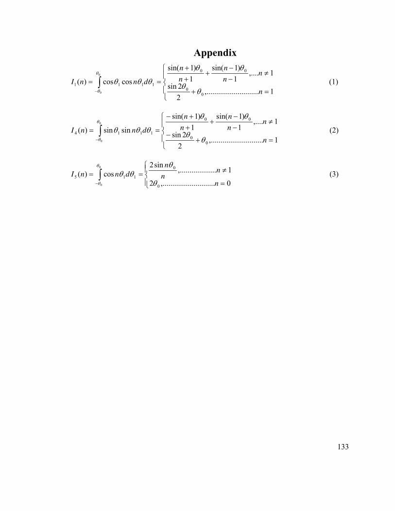
Appendix

∫− ⎪

⎩

⎪⎨

⎧

=+

≠−−

+++

==0

0 1..................,.........2

2sin

1,....1

)1sin(

1

)1sin(

coscos)(

00

00

1111

θ

θ θθ

θθ

θθθn

nn

n

n

n

dnnI (1)

∫− ⎪

⎩

⎪⎨

⎧

=+−

≠−−

+++−

==0

0 1..................,.........2

2sin

1,....1

)1sin(

1

)1sin(

sinsin)(

00

00

1114

θ

θ θθ

θθ

θθθn

nn

n

n

n

dnnI (2)

∫− ⎪⎩

⎪⎨⎧

=

≠==0

0 0..................,.........2

1..........,.........sin2

cos)(

0

0

115

θ

θ θ

θθθ

n

nn

n

dnnI (3)

133