Journal of Development Economics 97 (2012) 232–243

Contents lists available at ScienceDirect

Journal of Development Economics

j ourna l homepage: www.e lsev ie r.com/ locate /devec

Health shocks and consumption smoothing in rural households: Does microcredithave a role to play?☆

Asadul Islam a,⁎, Pushkar Maitra b

a Department of Economics, Monash University, Caulfield Campus, VIC 3145, Australiab Department of Economics, Monash University, Clayton Campus, VIC 3800, Australia

☆ We would like to thank the editor (Mark Rosenzwseminar participants at Monash University and theparticipants at the Econometric Society Australasianconference for their comments and suggestions. Puacknowledge funding provided by an Australian ReseThe usual caveat applies.⁎ Corresponding author.

E-mail addresses: Asadul.Islam@Buseco.monash.eduPushkar.Maitra@Buseco.monash.edu.au (P. Maitra).

0304-3878/$ – see front matter © 2011 Elsevier B.V. Adoi:10.1016/j.jdeveco.2011.05.003

a b s t r a c t

a r t i c l e i n f o

Article history:Received 23 June 2009Received in revised form 16 June 2010Accepted 16 May 2011

JEL classification:O12I10C23

Keywords:Health shocksMicrocreditConsumptionInsuranceBangladesh

This paper estimates, using a large panel data set from rural Bangladesh, the effects of health shocks onhousehold consumption and how access to microcredit affects households’ response to such shocks.Households appear to be fairly well insured against health shocks. Our results suggest that households selllivestock in response to health shocks and short term insurance is therefore attained at a significant long termcost. However microcredit has a significant mitigating effect. Households that have access to microcredit donot need to sell livestock in order to insure consumption. Microcredit organizations andmicrocredit thereforehave an insurance role to play, an aspect that has not been analyzed previously.

eig), two anonymous referees,University of Newcastle andMeetings and at the NEUDCshkar Maitra would like toarch Council Discovery Grant.

.au (A. Islam), 1 Even though micthe purposes of this

ll rights reserved.

© 2011 Elsevier B.V. All rights reserved.

1. Introduction

One of the biggest shocks to economic opportunities faced byhouseholds is major illness to members of the households. Whilehealth shocks can have adverse consequences for households in bothdeveloped and developing countries, they are likely to have aparticularly severe effect on households in the latter, because thesehouseholds are typically unable to access formal insurance markets tohelp insure consumption against such shocks.

The literature on the effects of health shocks on householdoutcomes in developing countries is quite large and the results are(surprisingly) mixed. Kochar (1995); Skoufias and Quisumbing(2005); and Townsend (1994) find that illness shocks are fairly wellinsured. Others (Asfaw & Braun, 2004; Beegle et al., 2008; Cochrane,1991; Dercon & Krishnan, 2000; Gertler & Gruber, 2002; Lindelow &

Wagstaff, 2007;Wagstaff, 2007) however find that illness shocks havea negative and statistically significant effect on consumption orincome. One general conclusion that could be drawn from the existingliterature is that the impact of health shocks is crucially dependent onthe ability of the households to insure against such shocks, which inturn is related to health and access to financialmarkets. Besley (1995),Fafchamps et al. (1998), Gertler and Gruber (2002), Jalan andRavallion(1999), Rosenzweig and Wolpin (1993), and Udry (1990)all reach essentially the same conclusion: wealthier households arebetter able to insure against income shocks in general and health/illness shocks in particular.

This implies that financial institutions could have an importantrole to play in insuring consumption against income shocks.Unfortunately commercial financial institutions in developing coun-tries are, more often than not, weak and do not adequately service thepoor. These institutions are typically not conveniently located, havesubstantial collateral requirements and impose large costs on savings(see Morduch, 1999). In contrast microfinance institutions holdsignificant promise. Microfinance programs are typically targeted atthe poor (and the near-poor), do not impose significant physicalcollateral requirements and actively promote savings.1

rofinance is wider in scope compared to microcredit, we will, forpaper, use the two terms interchangeably.

3 The evidence on, and the impact of, the use of livestock and other productiveassets from other parts of the world is mixed. Fafchamps et al. (1998) find limitedevidence that livestock inventory serve as buffer stock against large variation in cropincome induced by severe rainfall shock. They find that livestock sales compensate for15−30% of income shortfalls due to village level shock. On the other hand in theirstudy of consumption insurance and vulnerability in a set of developing andtransitional countries Skoufias and Quisumbing (2005) find that loss of livestock donot have a significant negative effect on the growth rate of consumption per-capita.Kazianga and Udry (2006) also find little evidence of the use of livestock as bufferstocks for consumption smoothing. Instead they find households rely exclusively onself-insurance in the form of adjustments to grain stocks to smooth out consumption.(Park, 2006) finds that households who do not live very close to other households selloff their livestock and other assets when they experience a shock, i.e., sell livestock inorder to smooth consumption in the absence of alternative social network basedmechanisms to smooth consumption.

4 The data was collected by the Bangladesh Institute for Development Studies (BIDS)for the Bangladesh Rural Employment Support Foundation with financial assistancefrom the World Bank. The first author was involved in the fourth round of datacollection, monitoring and writing the final report.

5 To be specific, the regression results presented in Cochrane (1991), Table 2, show

233A. Islam, P. Maitra / Journal of Development Economics 97 (2012) 232–243

The primary aim of this paper is to examine the potential role ofmicrocredit in enabling households to insure consumption againsthealth shocks. Microcredit can help smooth consumption in a numberof ways. It can help households diversify income and free up othersources of financing that can be used to directly smooth consumption.In several cases microfinance institutions (MFIs) have an explicitinsurance component associated with loans. Additionally, no collat-eral requirement for microcredit loans means that poor householdscan get loans more easily. Credit from microfinance organizationsplays a pivotal role in the daily life of households in rural Bangladesh.Pitt and Khandker, (1998) find that access to microfinance signifi-cantly increases consumption and reduces poverty. (Amin et al., 2003)find that poor households that join in a microcredit program tend tohave better access to insurance and smoothing devices compared tothose who do not. Morduch (1998) and Pitt and Khandker (2002)both find that microcredit can help smooth seasonal consumption.Their results indicate that household participation in microcreditprograms is partially motivated by the need to smooth the seasonalpattern of consumption and male labour supply.

There is very little prior research on the role of microcredit inenabling households to insure against income shocks in general andhealth shocks in particular. Gertler et al. (2009) is one of the fewexceptions in this respect. They use data from Indonesia and showthat microfinance institutions play an important role in helpinghouseholds self-insure against health shocks. Our paper builds on thisline of research. We use, in this paper a newly-available large andunique household-level panel dataset from Bangladesh, spanningabout 8 years, to examine the role of microcredit in enablinghouseholds insure against health shocks. We find that in generalhealth shocks do not have a significant effect on householdconsumption: households appear to be fairly well insured. But thatleads us to the possibly even more important question—whatinstitutions/arrangements enable households to insure against healthshocks? We focus on institutions that enable ex post consumptionsmoothing, since health shocks are shown to be unanticipated (seeSection 4.1 below) rendering ex ante consumption smoothingdifficult.2 While there are a large number of potential institutions, inthis paper we focus on access to credit, measured by the amount ofcredit from “other” sources including relatives, friends or informalmoney lenders; and purchase and sale of assets and livestock. Ourresults show that in general households donot increase their borrowingfrom “other” sources in response to long term health shocks. The mostcommon way households insure is by selling productive assets(livestock) when faced with adverse health shocks. It is here thatmicrocredit has a significant role to play: we find that householdshaving access tomicrocredit are less likely ornot likely to sell productiveassets (livestock) in response to idiosyncratic health shocks.

There now exists a significant volume of literature from develop-ing countries that finds that households use livestock (or productiveassets in general) to smooth consumption against income shocks.Rosenzweig and Wolpin, (1993) find that in rural India, bullocks,while also used as a sources of mechanical power in agriculturalproduction, are sold to smooth consumption in the face of incomeshocks. Consumption is therefore smoothed at the cost of cropproduction efficiency. The authors find that borrowing-constrainedhouseholds keep on average half of the optimal level of bullocks.(Jodha, 1978), again using data from India, argues that sales ofproductive assets when facedwith shocks (a drought in this case) is socommon that to outsiders it gives the false impression of “a low costand smooth process of evening out consumption levels operated byfarmers over a period of the famine cycle" (Jodha, 1978, Page A40).However the long term implications of such actions are quite severe,particularly in terms of production in the post-drought period. He also

2 See Morduch (1995) for more on ex ante and ex post consumption smoothing.

argues that the loss of productive assets during the drought reducesthe capacity of farmers to re-initiate farm activity on their own.3 Eventhough the specific shock that we consider in this paper is different,the main story remains. While it can have a positive effect onconsumption insurance in the short run, the sale of livestock and otherproductive assets can have significant welfare impacts in the long run.Using data from Bangladesh we find that access to microfinancereduces and often removes the requirement to sell livestock inresponse to health shocks. This is an aspect of microfinance that hasnot been addressed adequately in the literature.

2. Data and descriptive statistics

The paper uses three rounds of a household level panel data setfrom Bangladesh. This data is a part of a survey aimed at examiningthe effect of microcredit on household outcomes.While four rounds ofthe survey were conducted (in 1997–1998, 1998–1999, 1999–2000and 2004–2005), for purposes of this paper we use data from the first,third and fourth round of the surveys. The primary reason for ignoringthe second round, is that this survey round did not collectcomprehensive information on consumption.4 All the surveys wereconducted during the period December–March, which implies that itis unlikely that any of the results are driven by the timing of thesurvey. Many of the participants dropped out of the program for oneyear or more and some of the initial non-participants becameparticipants later.

The survey sampled around 3000 households in 91 villages spreadevenly throughout the country, selected to reflect the overall spread ofmicrocredit operations in Bangladesh. The attrition rate was low – lessthan 10 percent from the first to the fourth round. The final round ofsurvey consists of 2729 households in 91 villages. Because of missingdata on some key variables for 35 households, our final estimatingsample consists of a balanced panel of 2694 households. The surveycollected detailed information on a number of socio-economic variablesincluding household demographics, consumption, assets, income,health, education and participation in microcredit programs.

Previous research indicates that the measurement of the illnessshock variables is important in analysing the impact of illness on growthof consumption. Indeed the results can vary significantly depending onhow the health shock is measured. For example, Cochrane (1991) usingdata from the US shows that short spells of illness are well insured, …,but that very long spells are not fully insured (Cochrane, 1991, Page969).5 In this paper we use self-reported health shocks: respondents inour survey were asked about new or ongoing and past illness of allmembers in the household. We use this information to compute a

that the regression of consumption growth on daysN0 work loss dummy shows almostno effect of illness on consumption growth. However the regression of consumptiongrowth on the dummy days of illness≥100 gives a large and significant coefficientestimate.

234 A. Islam, P. Maitra / Journal of Development Economics 97 (2012) 232–243

number of differentmeasures of household level health shocks. The firstmeasure thatwe consider iswhether anymember of the householdwassick during the last 15 days prior to the survey. This measure, whilebeing simple to understand and compute is not particularly informativebecause of its binary nature. The problem is that an individual's self-reported health status is subjectively affected by an individual's socialand cultural background, given the individual's subjective health.Schultz and Tansel (1997) argue that this is because of “culturalconditioning": the threshold of what is considered good health variessystematically across a society, controlling for their objective healthstatus.6 They go on to argue that self-reported functional activitylimitations are better indicators of health status.7

Fortunately the survey also asks the respondents additionalquestions on their health status: number of days sick in the last15 days and the number of days amember had to refrain fromwork orincome earning activities if any member in the household was sick inthe last 15 days. The duration of sickness in the last 15 days is likely tocontain more information on health status compared to the simplebinary indicator (whether any member of the household was sickduring the last 15 days prior to the survey); but this is still notcomplete; again, the definition of sick could vary systematically acrossthe society. The third measure (time off work due to health shock inthe household) is possibly the best measure because here illness isconsidered severe enough to affect income earning activities of theindividual who is sick or of another member of the household whohad to refrain from work to take care of a member of the householdwho is sick, and is less likely to suffer from the cultural conditioningproblem.

The three measures of health shocks that we have discussed so farcould be viewed as measures of short-term health shocks. We alsoconsider two longer-term measures of health shocks: whether thehousehold incurred any big expenditure or loss of income due tosickness in the past one year and whether the main income earnerdied in the last one year. These two longer-term measures of healthshock are less likely to suffer from the cultural conditioning problemthat we have discussed above, as they are based on objective criterion.

The descriptive statistics presented in Table 1, Panel A show someinteresting and significant variations across the three rounds of datathat we use for purposes of our analysis. First, 49% of households in the1997–1998 survey report that some member was sick in the past15 days, this goes down to 44% in the 1999–2000 survey and furtherdown to 21% in 2004–2005.8 Average number of days lost in the past15 days due to illness varies from 3.1 in the 1997–1998 survey downto 1.36 in the 2004–2005 survey. The percentage of householdsexperiencing a large shock in expenditure in the last one year rangesfrom 15.7% in 1997–1998 to 22.6% in 2004–2005. Up to 1.5% ofhouseholds report death of the main earner in the family in the pastone year.

Table 1, Panel B presents descriptive statistics on other socio-economic and demographic characteristics of the household. Theaverage size of the household varies from 5.63 members in 1997–1998 to 7.23members in 2004–2005. The years of education attained by

6 Individuals who are more educated, are more wealthy and are from sociallyadvantaged groups are typically more aware of the limitations imposed on them bytheir health status and are more likely to report themselves (and their family) as beingof poor health.

7 Gertler et al. (2009) use measures of individuals’ physical abilities to performactivities of daily living (ADLs) such as bending and walking 5 km. ADLs are regardedas reliable and valid measures of physical functioning ability in both developed anddeveloping countries, and they distinguish the type of serious exogenous healthproblems that are likely to be correlated with changes in labour market andconsumption opportunities. Unfortunately we do not have information on suchvariables.

8 This large drop in short run sickness is quite surprising and unfortunately we donot have a very good explanation for this. It could be that 2004–2005 was aparticularly good year. We also cannot rule out reporting error or bias associated withanswering the same question repeatedly.

the most educated member of the household has increased from5.48 years in 1997–1998 to 7.27 years in 2004–2005. While theproportion of female headed households has doubled over the period1997–1998–2004–2005, the majority of households continue to bemale-headed.

The impact of illness shocks on consumption and the ability ofhouseholds (and other risk sharing institutions) to smooth consump-tion canvary fromone item toanother. Skoufias andQuisumbing (2005)find that adjustments in non-food consumption can act as amechanismfor partially insuring food consumption from the effects of incomechanges. So we use change in food and the change in non-foodconsumption expenditure as the two main outcome variables in ouranalysis. For each food item, households were asked about the amountthey had consumed out of purchases, out of own production and fromother sources in the reference period. The reference period for the fooditems differ depending on the type of food: some food items (e.g., beef,chicken) are consumed occasionally (once or twice in a month), whileothers (e.g., rice, lentil) are consumed much more frequently.Computing non-food consumption expenditure is much more prob-lematic. Non-food consumption is measured yearly since some of theitems are purchased occasionally. Our measure of non-food consump-tion expenditure includes items such as kerosene, batteries, soap,housing repairs, clothing, but excludes expenditure on items that arelumpy (e.g., dowry,wedding, costs of legal and court cases, etc.).Wealsoexclude expenditure on health and medical care. We aggregate allexpenditure in these two broad categories, and value it using the pricequoted by the household (unit value) since commodities differ in termsof quality.9 This way we obtain information on expenditure on food inthe last month prior to the survey.

Table 1, Panel C reports themean and standard deviation of food andnon-food consumption expenditure. Average household consumptionvaries from 2433 Taka (≈61 USD) in 1997–1998 to 3214 Taka(≈55 USD) in 2004–2005.10 There is considerable variation across thedifferent rounds with a big increase in expenditure on food between1997–1998 and 1999–2000. The share of non-food consumption(excluding health and medical expenditure) in total householdexpenditure is 21.1% in 1997–1998, which declined to 13.5% in 1999–2000 and thenwent back to 21.1% in 2004–2005. This reduction in non-food consumption expenditure in 1999–2000 could partly be attributedtomajor floods at the end of 1998,which affectedmost of the country.11

Table 2 presents selected descriptive statistics on credit demand andsupply. As of 1997–1998, asmany as 30% of households had taken someloan from relatives, friends, or others in the past one year andsurprisingly this number has decreased to 18% by 2004–2005. Theaverage amount of loan taken from other sources (in the past one year)has however increased consistently from 4657 Taka (≈116 USD) in1997–1998 to 9646 Taka (≈166 USD) in 2004–2005. Average amountof borrowing frommicrocredit organizations has also increased over therelevant time period: from 7427 Taka (≈186 USD) in 1997–1998 to11,682 Taka (≈201 USD) in 2004–2005. The percentage of householdswho borrowed for consumption purposes has fallen, as has thepercentage of households who borrowed to pay for medical expenses.

9 Price variation is at the item–household–year level. Households buy differentquality of food (e.g., coarse rice, fine rice, etc.) and it is difficult to monitor the price ofeach quality (actually impossible using the data we have at our disposal). We use datareported by households. However, where we find some inconsistencies (for example avery high or a very low value) we use the village level median price to convert thereported quantity into monetary value. The village level price information wascollected by a survey of village shopkeepers and this information was only used inspecial cases. These values are then deflated using the rural household agriculturalprice index (1997–1998=100).10 Taka is the currency of Bangladesh: 1 USD=40 Taka in 1998, 1 USD=44 Taka in2000 and 1 USD=58 Taka in 2005.11 Although 1999–2000 survey took place more than one year after the flood, a shockof that magnitude is likely to, and indeed did, have a fairly long-run effect onhousehold behaviour and outcomes.

13 The assumption of an exponential (CARA) utility function is not crucial to our

analysis. Assuming a CRRA utility function of the form u cits; θitsð Þ = c1−αits

1−αexp θitsð Þ

Table 1Household level descriptive statistics.

1997–1998 1999–2000 2004–2005

Mean Std. dev Mean Std. dev Mean Std. dev

Panel A: health shock variablesWhether any member was sick in last 15 days 0.492 0.500 0.438 0.496 0.211 0.408Number of days sick in last 15 days due to sickness 2.445 3.187 2.056 2.930 1.306 3.065Number of days work lost due to sickness 3.119 3.631 3.017 3.095 1.349 3.057Whether household incurred any big expenditure 0.157 0.402 0.144 0.352 0.226 0.419Death of the main earner in the family 0.010 0.012 0.010 0.101 0.015 0.121

Panel B: demographic variablesAge of the household head 44.52 13.36 46.81 13.34 47.75 12.20Working age population 2.81 1.38 3.02 1.53 3.59 2.12Household size 5.63 2.29 6.06 2.48 7.23 3.85Maximum education attained by any household member 5.48 4.13 6.23 4.07 7.27 6.53Arable land owner 68.47 146.66 80.79 159.03 73.68 225.92Number of children 2.83 1.66 2.22 1.46 3.01 2.39Number of women 2.66 1.40 2.94 1.52 3.26 2.00Number of elderly 0.25 0.49 0.39 0.60 0.31 0.54Number of married members 2.38 1.10 2.70 1.37 3.16 1.98Female headed household 0.05 0.23 0.05 0.23 0.11 0.31

Panel C: outcome variable (in Taka)Food consumption (monthly) 2432.8 1832.2 2949.5 2721.1 3214.4 3296.1Non-food consumption expenditure (yearly) 5628.2 6877.2 3499.4 7022.8 6024.0 9563.7Non-land asset (excluding livestock) 13,128.1 27,327.5 18,529.7 14,554.0 17,661.2 44,394.1Value of livestock 5956.2 7664.7 4027.5 6242.8 4296.7 7432.9Income 32,975.1 33,572.6 35,733.6 50,804.0 45,252.5 50,515.5Self-employment income 6009.8 104,059.0 5377.4 28,842.5 6788.1 63,987.5Medical expenditure 2191.5 10254.5 2015.7 8799.6 4295.1 12406.1Total non-food including medical expenditure (monthly) 651.6 1427.6 459.6 1318.5 859.9 1830.8Total expenditure 3084.5 3259.9 3409.0 4039.7 4074.3 5126.9Percentage of non-food in total expenditure 21.1 13.5 21.1Number of observations 2694 2694 2694

235A. Islam, P. Maitra / Journal of Development Economics 97 (2012) 232–243

Table 3 presents selected descriptive statistics on ownership oflivestock and non-land non-livestock assets, separately for thetreatment (microfinance recipient) and comparison (non-recipient)households. The percentage of households who own livestock ishigher for microfinance recipient households in each of the threesurvey years, as is the median value of livestock. This is not surprisingbecause MFIs encourage borrowers (microfinance recipients) toinvest in livestock. However the mean and median value of non-land non-livestock assets is higher for the comparison households,compared to the treatment households. The average savings (com-puted as income minus expenditure) of the two sets of households donot show any particular pattern. Part of this is possibly due to thefact that agricultural income is typically measured with error. Evenexpenditure is likely to be measured with error; after all this was ayearly survey (Lim & Townsend, 1998). We do not have detailed dataon expenditure over the year.

3. Estimation methodology

Complete risk sharing within the community will result in eachhousehold belonging to that community being protected fromidiosyncratic risk.12 Consumption will still vary but only because ofthe community's exposure to risk. The test for full consumptioninsurance is therefore a test of the validity of Pareto Optimality for theeconomy under consideration. Since the Pareto optimal consumptionallocations are derived from the social planner's problem, it turns outthat the planner needs to solve the following maximization problem:

Max∑i

∑t

∑s

μ isπsρtu cits; θitsð Þ ð1Þ

12 The degree of consumption insurance is defined as the extent to which change inhousehold consumption co-varies with change in household income.

subject to

∑i

cits = ∑i

yits∀t; s ð2Þ

where πs is the probability of state s ;s=1,…, S; cits householdconsumption; yits is household income; μ is is the time invariant Paretoweight associated with household i ; i=1,…, I in state s; ρ is the rateof time preference assumed to be the same for all households; θitsincorporates factors that change tastes. Finally I is the number ofhouseholds in the village. Assuming an exponential utility function13

u cits; θitsð Þ = − 1α

exp −α cits−θitsð Þf g ð3Þ

andmanipulating the first order conditions (and ignoring the notationfor the state) we get

Δcit = Δcat + Δθit−Δθat� � ð4Þ

where

Δcat =1I∑i

cit and Δθat =1I∑i

θit

Eq. (4) implies that under the assumption of full consumption insur-ance individual consumption cit depends only on the community/village

gives an estimating equation in log format as opposed to the specification that wepresent in Eq. (4). In this case the first order condition can be written as: Δ log citð Þ =Δcat + Δθit−Δθat

� �;Δcat = 1

I ∑i log citð Þ;Δθat = 1I ∑i θit .

Table 2Descriptive statistics. Microcredit and other loans (in Taka).

1997–1998 1999–2000 2004–2005

Mean Std. dev Mean Std. dev Mean Std. dev

Microcredit borrowingAmount of loan taken from microcredit organization 7427.3 7165.0 10,616.8 11,332.4 11,682.5 17,378.7Number of microcredit borrowers 1592 1532 1280

Borrowing from other sourcesPercentage of households taken loan in last month 5.18 4.3 NAAmount of loan taken in last month 167 2284.1 468.07 15573.2Percentage of households taken loan in last year 29.4 26.6 18Amount of loan taken in last year 4657.2 12,712.1 7350.7 28,640.3 9464.0 18,045.8Percentage of households who took loan from neighbours and relatives 53 35.1 NAPercentage of households who took loan for consumption 23.4 11.1 9.1Percentage of households who took loan for medical purpose 3.5 0.5 0.6

Monthly loan data is not available for the last round of survey 2004–2005.

236 A. Islam, P. Maitra / Journal of Development Economics 97 (2012) 232–243

level average consumption cta, especially since tastes/preferences are not

expected to change frequently.14

An empirical specification follows immediately. Regress thechange in the consumption of the ith household on the change inthe village level average consumption and other explanatory variables(for example socio-economic characteristics and health status ofhousehold members). Formally the empirical specification can bewritten as:

ΔCivt = α0 + α1Hivt + α2Xivt + βΔCavt + εivt ð5Þ

where ΔCivt is the change in (real) consumption of household i invillage v at time t; Hivt is the health shock faced by household i invillage v and time t. The error term εivt includes both preferenceshocks and measurement error and is distributed identically andindependently. The risk sharing model predicts that β=1 and α1=0,i.e., health shocks should have no role in explaining change inhousehold consumption.15 This way we can identify whether ruralhouseholds are vulnerable to transitory shocks such as illness shocks.

However Ravallion and Chaudhuri (1997) argue that this test(β=0 and α1=0 in Eq. (5)) gives biased estimates of the excesssensitivity parameter against the alternative of risk-market failurewhenever there is a common village level component in householdincome changes. They suggest (and this is the method that we use inthis paper) the use of the following specification:

ΔCivt = α0 + α1Hivt + α2Xivt + δv + μ t + δv × μ tð Þ + εivt ð6Þ

where δv represents village fixed effects; μ t represents the timeeffects; δv×μ t captures village-time interaction effects; εivt is thehousehold-specific error term capturing the unobservable compo-nents of household preferences. Since changes in consumption inresponse to health shocks (or for that matter any shock) are typicallycharacterized by substantial cross-household heterogeneity, weinclude in the set of explanatory variables a set of time varying

14 To examine how the Pareto Optimal allocation is attained in a decentralisedeconomy, we assume the existence of a complete set of Arrow–Debreu securities. Theexistence of such securities allows us to decentralise the economy and examinewhether full insurance can be attained through market mechanisms in such aneconomy. It can be shown that if there exists a complete set of Arrow–Debreusecurities, the equilibrium consumption allocation will be identical to that obtainedunder the social planner's problem.15 Notice that the empirical specification uses the change in consumption rather thanthe level of consumption as the dependent variable because in this way potentialomitted variable biases caused by the unobserved household characteristics can beavoided. Our model can therefore be viewed as the first-difference of a random growthmodel where we allow consumption growth to be different across the differentvillages.

controls at the household level (Xivt). Changes in village-levelconsumption values are accounted for by including village fixedeffects (δv). Without village fixed effects, the regression may yieldbiased estimates because of possible correlation between the omittedor unobserved village characteristics and the error term. It also allowsus to control for any aggregate or co-variate risks faced by allhouseholds in the village. The time dummies control for prices, andthe interaction of the time dummies with the village fixed effectsallows us to control for price changes that are village-specific overtime. They also enable us to control for village level shocks. In theregression results that we report below (see Section 4), all standarderrors are clustered at the village level.

If there is perfect risk sharing within the village then householdconsumption should not be sensitive to the idiosyncratic health shockHivt, once aggregate resources are controlled for, i.e., α1=0.

Now we turn to the potential effects of microcredit. To examinewhether microcredit plays a role in enabling households to insureagainst idiosyncratic shocks, we estimate an extended version ofEq. (6) as follows:

ΔCivt = β0 + β1Hivt + β2Xivt + β3 Hivt × Divtð Þ + δv + μ t

+ δv × μ tð Þ + εivt

ð7Þ

Here Divt is the treatment status of the household in a microcreditprogram and is measured by the amount borrowed. If households areunable to fully share the risk, then β1 will be less than zero, and thecoefficient of interaction of the treatment variable and the healthshock (β3) then represents the effect of microcredit on changes inconsumption.

A major concern in estimating Eq. (7) is that the estimatedcoefficient of β3 might be biased. This could be because of two reasons.The first is self-selection: some households might choose not toparticipate in the microcredit program. Additionally microcreditprograms are generally placed in selected villages. Fortunately, theavailability of panel data at the household level allows us toconsistently estimate the average treatment effect without assumingignorability of treatment because in this case, first differencing thedependent variable eliminates the bias caused by the time invariantunobservables. However one must be careful because this proceduredoes not eliminate the potential bias caused by the possibility that ahousehold's decision to participate depends on time varying un-observables, which in turn also affects the change in consumption. Ouruse of village fixed effects in the first-differenced model allows us toaccount for any further village-specific growth/shocks/unobservables.The impact of microcredit in mitigating health shocks is identified by

Table 3Descriptive statistics. Asset ownership for microcredit recipients and others.

1997–1998 1999–2000 2004–2005

Treatment Comparison Treatment Comparison Treatment Comparison

Percentage of households owning livestock 0.92 0.87 0.89 0.84 0.77 0.74Median value of livestock 3964.64 2105.29 1270.57 1060.30 968.18 731.03Mean value of non-land non-livestock asset 5812.58 11,486.35 14,167.00 15,025.18 10,418.21 17,796.65Median value of non-land non-livestock asset 915.39 1077.72 12,729.20 12,837.01 4743.32 5104.27Savings 3622.75 −4989.37 −469.60 −1909.29 2009.67 1459.27

237A. Islam, P. Maitra / Journal of Development Economics 97 (2012) 232–243

the difference between the treatment and the comparison householdsover time, conditional on controls.

The second reason for this bias is measurement error, which ariseslargely from the usual reporting problems. Measurement error ofthis kind would tend to induce an attenuation bias that biases thecoefficient towards zero. In this case, OLS estimates provide a lowerbound for the true parameters.16 With fixed effects estimation,measurement error is likely to exacerbate the bias. So, we estimate theeffects of microcredit on consumption smoothing using the instru-mental variable (IV) strategy to take into account of the possiblemeasurement error. Note that the IV method is also suitable iftreatment status is correlated with the time-varying unobservables.The microcredit organizations we study here typically offer credit toeligible households in the program village, defined as thosehouseholds that own less than half-acre land.17 We use a dummyvariable indicating whether or not the household is eligible in aprogram village as the instrument. To be more specific define E=1 ifthe household is eligible and 0 if not; P=1 if the household resides ina program village, 0 if not. The relevant instrument is P×E, whichtakes the value of 1if the household is eligible and resides in a programvillage. P×E is then a broad measure of eligibility.18 There is animportant issue to note here: the official eligibility criterion variesslightly across the different microcredit organizations and over time.Discussion with microcredit borrowers and local officials of micro-credit organizations indicate that there are no significant differencesamong the different microcredit organizations as far as the eligibilitystatus is concerned. However given that land quality differs widelyamong the different regions, a number of microfinance institutionshave in the recent years relaxed the land-based eligibility criterionslightly (i.e., households owning more than half acre of land are alsoeligible for microcredit). We account for this and our instrument istime varying: for the first survey round (1997–1998), our instrumentis whether household owns less than half-acre land or less.We changethis eligibility criterion to 0.75 acre for the 1999–2000 survey and to 1acre for the 2004–2005 survey.

How well does eligibility predict microcredit receipt? To examinethis question we present in Table 4 the results obtained fromregressing microcredit received by the household (Divt) on eligibility(P×E) and a set of other household characteristics. We present theresults corresponding to 3 different specifications: in specification 1the only variable included in the set of explanatory variables is

16 However, imputation errors in the construction of consumption variable andreporting error in credit variable may bias the credit coefficient upwards (Ravallion &Chaudhuri, 1997). For a positive coefficient, this bias is in the opposite direction of thestandard downward attenuation bias due to measurement errors and therefore the neteffect cannot be signed a priori.17 Credit is not available or offered to a household not living in a treatment(program) village.18 However, it is to be noted that the primary purpose of using IV estimation here isnot to tackle the endogeneity of program participation. It is more to address the issueof possible measurement error in the credit variable. Moreover, we control for theamount of arable land the household owns in our regressions so any effect ofownership of land on consumption or other outcome is directly accounted for. Theexclusion restriction is the following: conditional on land-ownership and other socio-economic characteristics of the household, eligibility is independent of outcomes,given participation.

eligibility (P×E); in specification 2, we include a set of householdcharacteristics in addition to eligibility; and finally in specification 3we include a full set of village fixed effects, time fixed effects andvillage-time interaction fixed effects. Irrespective of the specification,the eligibility (P×E) variable is positive and statistically significant,implying that eligibility is a good predictor for loan receipts.

Before proceeding further it is worth re-iterating that we use twodifferent outcomemeasures: change in food consumption and changein non-food consumption (excluding medical/health expenditure).Remember also that we use a number of different measures of healthshock. They are:

• Short-term measures of health shock:– Whether any member of household was sick during the last

15 days prior to survey (binary variable);– The number of days sick in the last 15 days for all working age

members of household;– The number of days amember had to refrain fromwork or income

earning activities if any member in the household was sick in thelast 15 days.

• Long term measures of health shock:– Whether the household incurred any big expenditure or loss of

income due to sickness in the past one year (binary variable);– Whether the main income earner died in the last one year (binary

variable).

4. Estimation results

4.1. Are health shocks persistent?

The estimation methodology that we use in this paper (seeSection 3) depends, crucially, on the assumption that health shocksare unpredictable and idiosyncratic in nature. Before we proceed tothe results, we examine the validity of this assumption. In particularwe examine whether households that experience health shocks in thecurrent period are more likely to receive health shocks in the futurei.e., whether health shocks are correlated over time. (Morduch, 1995)points out that if an income shock can be predicted beforehand, thenhouseholds might side-step the problem by engaging in costly ex antesmoothing strategies (e.g. diversifying crops, plots and activities). Thedata in such a situation would (incorrectly) reveal that income shocksdo not matter.

To examine the issue of whether health shocks are persistentor not, we estimate the following regression (see for example (Beegleet al., 2006)):

Hit = δi + λHit−1 + πXit + εit ð8Þ

Here Hit is some measure of health shock. The coefficient ofinterest is λ. If shocks are not persistent, i.e., households experiencinga shock in period t−1 are not significantly more likely to experience ashock in period t, then λ will not be statistically significant. Eq. (8) isestimated as a fixed effect logit, with survey round dummies. Thecoefficient estimates (using 3 different shock variables) are presentedin Table 5. None of the coefficient estimates are statistically significant

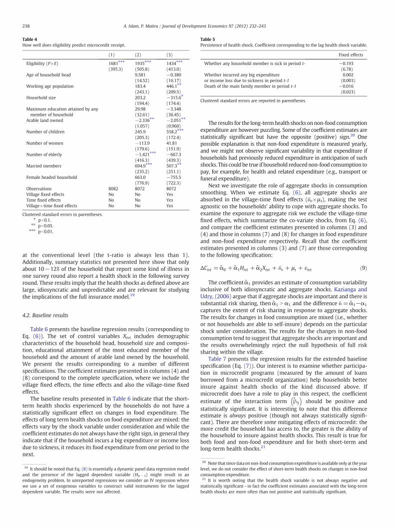
Table 4How well does eligibility predict microcredit receipt.

(1) (2) (3)

Eligibility (P×E) 1681⁎⁎⁎ 1935⁎⁎⁎ 1434⁎⁎⁎

(395.3) (505.8) (413.0)Age of household head 9.581 −0.380

(14.52) (16.17)Working age population 183.4 446.1⁎⁎

(243.1) (209.5)Household size 203.2 −315.6⁎

(194.4) (174.4)Maximum education attained by anymember of household

29.98 −3.348(32.61) (36.45)

Arable land owned −2.336⁎⁎ −2.051⁎⁎

(1.057) (0.960)Number of children 245.9 558.2⁎⁎⁎

(205.3) (172.4)Number of women −113.9 41.81

(179.6) (151.9)Number of elderly −1,421⁎⁎⁎ −667.3

(416.3) (439.3)Married members 694.9⁎⁎⁎ 507.3⁎⁎

(235.2) (251.1)Female headed household 663.0 −755.5

(776.9) (722.3)Observations 8082 8072 8072Village fixed effects No No YesTime fixed effects No No YesVillage×time fixed effects No No Yes

Clustered standard errors in parentheses.⁎ pb0.1.

⁎⁎ pb0.05.⁎⁎⁎ pb0.01.

Table 5Persistence of health shock. Coefficient corresponding to the lag health shock variable.

Fixed effects

Whether any household member is sick in period t- −0.193(6.78)

Whether incurred any big expenditure 0.002or income loss due to sickness in period t-1 (0.003)Death of the main family member in period t-1 −0.016

(0.023)

Clustered standard errors are reported in parentheses.

238 A. Islam, P. Maitra / Journal of Development Economics 97 (2012) 232–243

at the conventional level (the t-ratio is always less than 1).Additionally, summary statistics not presented here show that onlyabout 10−12% of the household that report some kind of illness inone survey round also report a health shock in the following surveyround. These results imply that the health shocks as defined above arelarge, idiosyncratic and unpredictable and are relevant for studyingthe implications of the full insurance model.19

4.2. Baseline results

Table 6 presents the baseline regression results (corresponding toEq. (6)). The set of control variables Xivt includes demographiccharacteristics of the household head, household size and composi-tion, educational attainment of the most educated member of thehousehold and the amount of arable land owned by the household.We present the results corresponding to a number of differentspecifications. The coefficient estimates presented in columns (4) and(8) correspond to the complete specification, where we include thevillage fixed effects, the time effects and also the village-time fixedeffects.

The baseline results presented in Table 6 indicate that the short-term health shocks experienced by the households do not have astatistically significant effect on changes in food expenditure. Theeffects of long term health shocks on food expenditure are mixed: theeffects vary by the shock variable under consideration and while thecoefficient estimates do not always have the right sign, in general theyindicate that if the household incurs a big expenditure or income lossdue to sickness, it reduces its food expenditure from one period to thenext.

19 It should be noted that Eq. (8) is essentially a dynamic panel data regression modeland the presence of the lagged dependent variable (Hit−1) might result in anendogeneity problem. In unreported regressions we consider an IV regression wherewe use a set of exogenous variables to construct valid instruments for the laggeddependent variable. The results were not affected.

The results for the long-termhealth shocks onnon-food consumptionexpenditure are however puzzling. Some of the coefficient estimates arestatistically significant but have the opposite (positive) sign.20 Onepossible explanation is that non-food expenditure is measured yearly,and we might not observe significant variability in that expenditure ifhouseholds had previously reduced expenditure in anticipation of suchshocks. This couldbe true if household reducednon-food consumption topay, for example, for health and related expenditure (e.g., transport orfuneral expenditure).

Next we investigate the role of aggregate shocks in consumptionsmoothing. When we estimate Eq. (6), all aggregate shocks areabsorbed in the village-time fixed effects (δv×μ t), making the testagnostic on the households’ ability to cope with aggregate shocks. Toexamine the exposure to aggregate risk we exclude the village-timefixed effects, which summarize the co-variate shocks, from Eq. (6),and compare the coefficient estimates presented in columns (3) and(4) and those in columns (7) and (8) for changes in food expenditureand non-food expenditure respectively. Recall that the coefficientestimates presented in columns (3) and (7) are those correspondingto the following specification:

ΔCivt = α̃0 + α̃1Hivt + α̃2Xivt + δv + μ t + εivt ð9Þ

The coefficient α̃1 provides an estimate of consumption variabilityinclusive of both idiosyncratic and aggregate shocks. Kazianga andUdry, (2006) argue that if aggregate shocks are important and there issubstantial risk sharing, then α̃1 N α1 and the difference δ = α̃1−α1

captures the extent of risk sharing in response to aggregate shocks.The results for changes in food consumption are mixed (i.e., whetheror not households are able to self-insure) depends on the particularshock under consideration. The results for the changes in non-foodconsumption tend to suggest that aggregate shocks are important andthe results overwhelmingly reject the null hypothesis of full risksharing within the village.

Table 7 presents the regression results for the extended baselinespecification (Eq. (7)). Our interest is to examine whether participa-tion in microcredit programs (measured by the amount of loansborrowed from a microcredit organization) help households betterinsure against health shocks of the kind discussed above. Ifmicrocredit does have a role to play in this respect, the coefficientestimate of the interaction term β̂3

� �should be positive and

statistically significant. It is interesting to note that this differenceestimate is always positive (though not always statistically signifi-cant). There are therefore some mitigating effects of microcredit: themore credit the household has access to, the greater is the ability ofthe household to insure against health shocks. This result is true forboth food and non-food expenditure and for both short-term andlong-term health shocks.21

20 Note that since dataonnon-food consumption expenditure is available only at the yearlevel, we do not consider the effect of short-term health shocks on changes in non-foodconsumption expenditure.21 It is worth noting that the health shock variable is not always negative andstatistically significant - in fact the coefficient estimates associated with the long-termhealth shocks are more often than not positive and statistically significant.

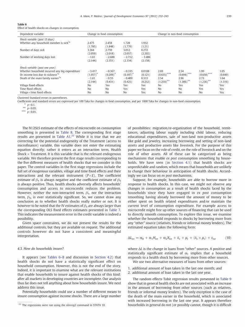
Table 6Effect of health shocks on changes in consumption.

Dependent variable Change in food consumption Change in non-food consumption

Shock variable (past 15 days)Whether any household member is sick?a 2.475 2.458 1.728 1.932

(1.785) (1.848) (1.770) (1.21)Number of days sick 3.364 2.759 3.012 0.272

(2.059) (2.018) (2.057) (2.202)Number of working days lost −1.61 −2.688 −2.712 −3.486

(2.144) (2.351) (2.334) (2.158)

Shock variable (past one year)Whether household incurred any big expenditure −3.417 −0.367 −0.335 0.0188 2.69 2.54 1.99 1.05Or income loss due to sickness?a (1.957)⁎ (0.209)⁎ (0.197)⁎ (0.121) (0.635)⁎⁎⁎ (0.694)⁎⁎⁎ (0.658)⁎⁎⁎ (0.649)Death of the main family earner?a −1.61 −0.55 −0.409 0.312 2.54 2.96 2.73 1.64

(2.144) (0.431) (0.425) (0.252) (1.259)⁎⁎ (1.306)⁎⁎ (1.236)⁎⁎ (1.316)Village fixed effects No Yes Yes Yes No Yes Yes YesTime fixed effects No No Yes Yes No No Yes YesVillage×time fixed effects No No No Yes No No No Yes

Clustered Standard errors in parentheses.Coefficients and standard errors are expressed per 100 Taka for changes in food consumption, and per 1000 Taka for changes in non-food consumption.

⁎ pb0.1.⁎⁎ pb0.05.⁎⁎⁎ pb0.01.

239A. Islam, P. Maitra / Journal of Development Economics 97 (2012) 232–243

The IV/2SLS estimate of the effects of microcredit on consumptionsmoothing is presented in Table 8. The corresponding first stageresults are presented in Table A1.22 While it is true that we arecorrecting for the potential endogeneity of the Treatment (access tomicrofinance) variable, this variable does not enter the estimatingequation directly; rather it enters as an interaction term, HealthShock × Treatment. It is this variable that is the relevant endogenousvariable. We therefore present the first stage results corresponding tothe five different measures of health shocks that we consider in thispaper. The control variables in the first stage regressions include thefull set of exogenous variables, village and time fixed effects and theirinteractions and the relevant instrument (P×E). The coefficientestimate of β1 is always negative and the coefficient estimate of β3

is always positive. Thus, health shocks adversely affects households’consumption and access to microcredit reduces the problem.However, neither the non-interacted term, β1, nor the interactionterm, β3, is ever statistically significant. So, we cannot draw anyconclusion as to whether health shocks really matter or not. It ishowever to be noted that the IV estimates of β3 are always larger thanthe corresponding OLS fixed effects estimates presented in Table 7.This indicates the measurement error in the credit variable is indeed apossibility.

Given space constraints, we do not present the results for theadditional controls, but they are available on request. The additionalcontrols however do not have a consistent and meaningfulinterpretation.

4.3. How do households insure?

It appears (see Tables 6–8 and discussion in Section 4.2) thathealth shocks do not have a statistically significant effect onhousehold consumption. However, this is not the end of the story.Indeed, it is important to examine what are the relevant institutionsthat enable households to insure against health shocks of this kind:after all markets in developing countries are incomplete. Our analysisthus far does not tell anything about how households insure. We nextaddress this issue.

Potentially households could use a number of different means toinsure consumption against income shocks. There are a large number

22 The regressions were run using the xtivreg2 command in STATA 10.

of possibilities: migration/re-organization of the household, remit-tances, adjusting labour supply including child labour, reducingeducational expenditures, sale of non-land non-productive assetslike gold and jewelry, increasing borrowing and setting of non-landassets and productive assets like livestock. For the purpose of thispaper we focus on the role of credit, on the role of livestock and on therole of other assets. All of these can be categorized as beingmechanisms that enable ex post consumption smoothing by house-holds. We have seen (in Section 4.1) that health shocks areunpredictable and random, whichmeans that households are unlikelyto change their behaviour in anticipation of health shocks. Accord-ingly we can focus on ex post mechanisms.

Suppose, for example, households are able to borrow more inresponse to health shocks. In this case, we might not observe anychanges in consumption as a result of health shocks faced by thehouseholds since they have engaged in ex post consumptionsmoothing having already borrowed the amount of money to beeither spent on health related expenditures and/or maintain thecurrent level of consumption expenditure. For example access tomicrocredit might free up other sources of financing that can be usedto directly smooth consumption. To explore this issue, we examinewhether the household responds to shocks by borrowing more fromany “other” source (relatives, friends or informal money lenders). Theestimated equation takes the following form:

ΔLivt = α0 + α1Hivt + α2Xivt + δv + μ t + δv × μ tð Þ + εivt ð10Þ

where ΔL is the change in loans from “other” sources. A positive andstatistically significant estimate of α1 implies that a householdresponds to a health shock by borrowing more from other sources.

We use two alternative measures of loans from other sources:

1. additional amount of loan taken in the last one month; and2. additional amount of loan taken in the last one year.

The random effects Tobit regression results presented in Table 9show that in general health shocks are not associated with an increasein the amount of borrowing from other sources (such as relatives,friends or informal money lenders). The only exception is the case ofthe death of the main earner in the household, which is associatedwith increased borrowing in the last one year. It appears thereforehouseholds in general do not (or possibly cannot, though it is difficult

Table 7Effect of health shocks on changes in consumption and the mitigating effects of microcredit.

Dependent variable Change in food consumption Change in non-food consumption

Shock variable (past 15 days)Whether any household member is sick 1.76 1.79 0.88 1.08

(1.89) (1.96) (1.95) (1.51)Shock×treatment 1.3 1.21 1.38 1.392

(0.05)⁎⁎ (0.53)⁎⁎ (0.53)⁎⁎ (0.99)Joint test F-statistic 0.87 0.84 0.2 0.51Number of days sick 0.02 0.02 0.02 −0.01

(0.02) (0.02) (0.02) (0.03)Shock×treatment 0.01 0.01 0.01 0.01

(0.00) (0.00)⁎ (0.00)⁎ (0.01)Joint test F-statistic 1.05 0.55 0.65 0.12Number of working days lost −0.03 −0.03 −0.02 −0.05

(0.02) (0.024) (0.02) (0.02)⁎⁎

Shock×treatment 0.02 0.02 0.02 0.03(0.02) (0.02) (0.02) (0.02)

Joint test F-statistic 1.31 2.07 2.48 4.96⁎⁎

Shock variable (past one year)Whether household incurred any bigexpenditure or income loss due to sickness

−3.55 −3.68 −3.44 −0.65 2.49 2.36 1.95 1.18(2.02)⁎ (2.12)⁎ (2.02)⁎ (1.27) (0.68)⁎⁎⁎ (0.74)⁎⁎⁎ (0.70)⁎⁎⁎ (0.68)⁎

Shock×treatment 0.16 0.10 0.11 0.87 0.23 0.21 0.10 −0.14(0.36) (0.40) (0.41) (0.78) (0.16) (0.17) (0.25) (0.24)

Joint test F-statistic 3.09⁎ 3.01⁎ 2.9⁎ 0.27 13.6⁎⁎⁎ 10.3⁎⁎⁎ 7.82⁎⁎⁎ 3.05⁎

Death of the main family earner −1.82 −1.73 −1.63 0.78 2.61 2.62 2.46 1.49(4.21) (4.42) (4.42) (2.869) (1.34)⁎ (1.36)⁎ (1.36)⁎ (1.43)

Shock×treatment 1.46 1.15 1.20 2.32 −0.66 0.33 0.26 0.14(9.03) (1.88) (1.86) (1.18) (0.39) (0.28) (0.26) (0.27)

Joint test F-statistic 0.19 0.15 1.14 0.07 3.77⁎ 3.69⁎ 3.86⁎ 1.09Village fixed effects No Yes Yes Yes No Yes Yes YesTime fixed effects No No Yes Yes No No Yes YesVillage×time fixed effects No No No Yes No No No Yes

Clustered Standard errors in parentheses.Regressions include full set of additional controls.Coefficients and standard errors are expressed per 100 Taka for changes in food consumption, and per 1000 Taka for changes in non-food consumption.

⁎ pb0.1.⁎⁎ pb0.05.⁎⁎⁎ pb0.01.

240 A. Islam, P. Maitra / Journal of Development Economics 97 (2012) 232–243

to make the distinction using the data at our disposal) use borrowingfrom other sources to insure against income shocks.

Households can also insure consumption by selling productive (forexample livestock) or non-productive assets (for example consumerdurables).23 Households that have access to microcredit might havefocusedonasset building/accumulation andon the creationor expansionof oneormore incomegenerating activities compared tohouseholds thatdonot. Similarly, livestock is a very important asset in rural Bangladesh.Alarge fraction of the households in our sample save in the form ofinvestment in livestock. Almost all the households own some livestock(e.g., cows, goats, chicken, ducks, etc.). As described in the introduction,there is also a significant volume of literature from developing countriesthat finds that households use livestock (or productive assets in general)to smooth consumption against income shocks.

To examine the issue of how purchase and sale of assets andlivestock is used to smooth consumption in response to health shocks,we estimate an equation similar to Eq. (7): the only difference beingthat here the dependent variable is the change in the values of assetsowned by the household. The estimated equation is:

ΔAivt = β0 + β1Hivt + β2Xivt + β3 Hivt × Divtð Þ + δv + μt

+ δv × μ tð Þ + εivt

ð11Þ

23 The value of consumer durables is the aggregated current market value of itemslike radio, fans, boats and pots that are owned by the household. The information onthe stock of assets is available only at the year level. Specifically the question was: Listif you have any of the following assets (give list). If yes, then please tell us how muchdid it cost to buy, and what would be the approximate value at present. We used the“value at present”. Households picked from the list of assets provided.

Here ΔAivt measures the change in the value of non-land asset orlivestock owned over two successive rounds of the survey. A negativeand statistically significant β1 implies that the household reduces itsownership of assets or livestock in response to a health shock. Apositive and statistically significant β3 implies that access tomicrocredit reduces the impact of the health shock and householdsdo not need to take re-course to sale of assets to insure against healthshocks.

The 2SLS and OLS fixed effects estimates of the mitigating effects ofmicrocredit on sale of assets and livestock are presented in Table 10.24

While the coefficient estimates of β1 and β3 do not have a systematicpattern in the case of change in ownership of non-land assets, those forthe change in ownership of livestock are much more systematic. Thecoefficient estimate associated with the health shock variable (β1) isalways negative and generally statistically significant in the change invalue of livestock regressions. In addition, the interaction term (β3) isgenerally positive and statistically significant. The effect of microcrediton the change in the value of livestock owned is given by β̂3. A positiveand statistically significant β̂3 in implies that, for a household thatreceives a health shock, an increase in the amount of microcreditavailable increases the value of livestock owned by the household. Theeffect of health shock is given by β̂1 + β̂3 × Treatment, which in turndepends on the amount of microcredit received. β̂1 then gives us thedirect effect of health shock, conditional on the household not receivingany microcredit. Now to interpret the results in column 4, Table 10, forhouseholds that do not receive any microcredit, the presence of a sickmember in the household reduces ownership of livestock by

24 The first stage results are again given by those presented in Table A1.

Table 82SLS estimates of the effect of health shocks on changes in consumption and themitigating effects of microcredit.

Dependent variable Change in

Foodexpenditure

Non-foodexpenditure

Shock variable (past 15 days)Whether any household member is sick −6.23

(9.31)Shock×treatment 13.38

(15.17)Joint test F-statistic 0.44Number of days sick −0.86

(1.32)Shock×treatment 0.51

(0.79)Joint test F-statistic 0.43Number of working days lost −0.28

(0.28)Shock×treatment 0.59

(0.69)Joint test F-statistic 0.93

Shock variable (past one year)Whether household incurred any big expenditure orincome loss due to sickness

−14.57 −16.13(18.3) (19.29)

Shock×treatment 18.78 21.81(23.5) (24.44)

Joint test F-statistic 0.63 0.70Death of the main earner in the family −37.69 −41.93

(45.55) (34.17)Shock×treatment 39.56 43.11

(44.9) (38.62)Joint test F-statistic 0.64 1.15

Each regression also incorporates village fixed effects, time effects and their interactions.Regressions include full set of additional controls.Coefficients and standard errors are expressed per 100 Taka for changes in foodconsumption and per 1000 Taka for changes in non-food consumption.

Table 9Effect of health shocks on loans from other sources.

Amount of loan takenin last one month('00 Taka)a

Amount of loan takenin last one year(in '000 Taka)b

Shock variable (past 15 days)Whether any householdmember is sick

3.51(3.842)

Number of days sick 0.04(0.0779)

Number of working days lost −2.06(5.531)

Shock variable (past one year)Whether household incurred anybig expenditure or income lossdue to sickness

0.41(1.013)

Death of the main earner in thefamily

2.40(1.1374)**

Clustered Standard errors are reported in parentheses.Regressions include full set of additional controls.a Using the first two rounds of survey data.b Using all 3 rounds of survey data.**pb0.05.

241A. Islam, P. Maitra / Journal of Development Economics 97 (2012) 232–243

7.94 thousand Taka. For the household receiving the average amountof microcredit (approximately 10,000 Taka), the change in the valueof livestock owned is − 7.94+12.97=5.03 thousand Taka(≈106.27 USD); i.e., actually increases ownership of livestock by5.03 thousand Taka.25 This total effect is however not always positive.To take another example, for households that do not receive anymicrocredit, the death of the main income earner reduces livestockownership by 38.59 thousand Taka. For the households receiving theaverage amount of microcredit, the change in the value of livestockowned (following the death of the main income earner) is −38.59+36.27=−2.32 thousand Taka (≈−49 USD), and this total effect isnegative but statistically significant (the joint test β̂1 + β̂3 = 0 isrejected). The remaining estimates can be interpreted in the sameway.

There is therefore a significant mitigating effect of microcredit. Inall cases the health shock variable β̂1

� �is negative and generally

statistically significant; the interaction term β̂3

� �is always positive

and generally statistically significant and in several cases the totaleffect β̂1 + β̂3

� �is actually positive and statistically significant (this

of course depends on the specific shock that we consider). Householdshaving access to microcredit either do not have to sell livestock orhave to sell less livestock in response to idiosyncratic health shocks.While households cannot explicitly borrow from MFIs for insurancepurposes, it is clear that access tomicrofinance gives households somefreedom to re-organize funds within the household leading to theobserved outcome that these households do not need to sell theproductive asset (livestock) either at all or to the extent that the nonrecipients need to. Unfortunately we do not have detailed data onexpenditure over the year to answer the question where the trade-off

25 We have assumed an exchange rate of 1USD=47.33 Taka.

happens. What is clear however is that over the long term, themicrocredit recipient households benefit, relative to the non-recipienthouseholds.

We examine the robustness of these results using the propensityscore matching method, where we match households on the basis oftheir socio-economic status and we restrict our analysis to thematched sample. This controls for heterogeneity in initial socio-economic conditions that may be correlated with subsequent healthshocks and the path of consumption growth.26 Regression conductedon the matched sample again show that the strongest effects are interms of changes in livestock owned. The regression results(presented in Table A2), show that the magnitude of the healthshock coefficients are, in general, larger using the matched sample,compared to the full sample. For example the 2SLS results for changein ownership of livestock presented in column 4, Table A2 implythat conditional on the household not receiving any microcredit,the household responds to any member being sick by reducingthe value of livestock owned by 9.5 thousand Taka (comparedto 7.94 thousand Taka for the full sample). For the householdreceiving the average amount of microcredit, the change in theamount of livestock owned is −9.50+17.88=8.38 thousand Taka(≈177 USD), more than what we obtained for the full sample(Table 10, column 4).

Households with access to microcredit therefore do not eitherneed to reduce their ownership of livestock or do not need to reduce itby as much in response to health shock (irrespective of how the shockis defined). Access to microcredit then helps in two different ways.First, in the short run, it helps insure consumption (see Table 7). Thiseffect is however not particularly strong. Second, recipient householdsdo not need to sell livestock, or do not need to sell livestock to theextent non recipient households need to, in response to health shocksand therefore insurance does not come at the cost of productionefficiency. There is therefore both a short run (direct) and a long-run(somewhat indirect) impact of microcredit. Despite a fairly largeliterature on the impact of microfinance (see Morduch, 1998; Pitt &Khandker, 1998; Pitt & Khandker, 2002; and Roodman & Morduch,2009) for quasi experimental research and (Banerjee et al., 2009;Karlan & Zinman, 2010) for experimental evidence), the existingliterature has not focused on role microcredit plays in terms of

26 See Islam and Maitra (2009) for more on the methodology used.

Table 10Effect of health shocks on change in ownership of assets and livestock.

Change in assets Change in livestock

OLS 2SLS OLS 2SLS

Shock variable (past 15 days)Whether any householdmember is sick

0.05 −7.94(0.22) (4.66)⁎

Shock×treatment −0.01 12.97(0.14) (7.54)⁎

Joint test F-statistics 0.05 2.9⁎

Number of days sick 0.00 −0.79(0.01) (0.90)

Shock×treatment 0.00 0.48(0.00)⁎⁎⁎ (0.54)

Joint test F-statistics 0.21 0.77Number of working days lost −0.00 −0.22

(0.00) (0.13)⁎

Shock×treatment 0.00 0.54(0.00) (0.31)⁎

Joint test F-statistics 0.1 3.02⁎

Shock variable (past one year)Whether household incurredany big expenditure

3.01 −11.58 −0.19 −15.20

Or income loss due to sickness (1.23)⁎⁎ (22.56) (0.23) (12.24)Shock×treatment 0.54 20.85 0.06 19.11

(0.67) (30.32) (0.07) (15.52)Joint test F-statistics 5.97⁎⁎ 0.29 0.72 1.54Death of the main family earner −2.47 −46.80 −1.84 −38.59

(2.68) (52.66) (0.58)⁎⁎ (18.86)⁎⁎

Shock×treatment −2.93 40.87 −0.09 36.27(1.20)⁎⁎ (51.90) (0.29) (18.60)⁎

Joint test F-statistics 0.85 0.84 10.15⁎⁎⁎ 4.18⁎⁎

Clustered Standard errors are reported in parentheses.Regressions include Village fixed effects, Time fixed effects and Village×time fixedeffects.Regressions include full set of additional controls.Coefficients and standard errors are expressed per 1000 Taka for changes in assets andlivestock.

⁎ pb0.1.⁎⁎ pb0.05.⁎⁎⁎ pb0.01.

Table A1First stage results corresponding to IV results presented in Table 8.

1 2 3 4 5

Eligibility (P×E) 742.4⁎⁎ 20,114⁎ 17,290⁎⁎ 506.8⁎⁎ 264.7⁎

(315.6) (12,302) (,508) (211.7) (143.3)Health shock 6154⁎⁎⁎ 16,637 −518.3 7860⁎⁎⁎ 10,111⁎⁎⁎

(702.8) (13,260) (796.4) (1,110) (2,835)Age of household head −6.409 1267 −378.9 −9.081 −3.276

(12.63) (1,193) (497.1) (12.11) (3.650)Working agepopulation

−99.40 16,967 −4867 301.3 142.0(297.6) (16,022) (9246) (220.1) (87.89)

Household size 225.8 −3144 9829 −182.3 −96.52⁎

(214.4) (4605) (7807) (158.0) (57.12)Maximum educationattained by any

−31.10⁎⁎⁎ 408.2 −447.3 10.402 5.286

Member of household (15.76) (732.3) (744.4) (22.68) (4.889)Arable land owned −0.102 −2.190 −7.805 −0.459 0.771

(1.002) (8.831) (19.60) (0.984) (0.931)Number of children −160.3 3360 −4229 201.4 169.7

(274.0) (5,940) (8,865) (262.5) (129.5)Number of workingage females

−105.4 −15,230 −4547 1.082 20.10(167.9) (12,592) (3647) (105.0) (46.07)

Number of elderly −552.6⁎⁎⁎ −8182 6322 −8.671 −85.78(321.6) (10,464) (10,396) (251.9) (75.63)

Number married 373.8⁎⁎⁎ −2595 7390 262.5 32.24(203.8) (11,124) (5959) (171.8) (67.79)

Female headedhousehold

−23.16 −13,239 2321 −292.8 23.09(475.1) (25,534) (13,009) (858.5) (115.3)

Constant −305.1 −70,039 21,343 −130.4 −527.9(1017) (71,396) (27,566) (812.8) (521.5)

Observations 5378 5378 5378 5378 5378R2 0.122 0.153 0.045 0.158 0.161F(1,.) 4.42 0.83 3.87 3.6481 5.44ProbNF 0.0355 0.3629 0.0492 0.057 0.0197Partial R2 0.0009 0.0002 0.0007 0.000681 0.0011

Regressions include Village fixed effects, Time fixed effects and Village×time fixedeffects.Standard errors in parentheses.Dependent Variables:

1. Whether any household member is sick×treatment.2. Number of days sick×treatment.3. Number of working days lost×treatment.4. Whether household incurred any big expenditure or income loss due to

sickness×treatment.5. Death of main earner in the family×treatment.⁎ pb0.1.

⁎⁎ pb0.05.⁎⁎⁎ pb0.01.

242 A. Islam, P. Maitra / Journal of Development Economics 97 (2012) 232–243

providing insurance in the manner we discuss here. An examinationof the role of microcredit in terms of providing insurance againstshocks is an important contribution of this paper.

5. Conclusion

This paper examines, using a large panel data set fromBangladesh, the ability or otherwise of poor households to insureagainst idiosyncratic and unanticipated health shocks. Is there a rolefor microcredit in this respect? Our results show that householdsthat have borrowed from microcredit organizations appear to bebetter able to cope with health shocks. The primary instrumentthrough which households insure is by trading in livestock.Households that have access to microcredit do not need to selllivestock or do not have to, to the extent households that do nothave access to microcredit need to, in order to insure consumptionagainst health shocks.

On a broader and quite a positive note, credit markets (of whichmicrocredit is one aspect) appears to be play a significant role ininsuring households against income fluctuations. This is nothingnew—there is evidence from a number of different developingcountries around the world regarding the role of credit markets inproviding insurance. Munshi and Rosenzweig, (2009) show using apanel data set from India that nearly one-quarter of the households inthe sample participated in the insurance arrangement in the yearprior to each survey round, giving or receiving transfers (broadly

classified into gifts and loans). Although loans account for just 20percent of all within-caste transactions by value, they are moreimportant than bank loans or moneylender loans in smoothingconsumption and in particular for meeting contingencies such asillness and marriage. They go on to argue that (in the context of ruralIndia) such within-caste loans are actually more important thanmicrocredit. The institutional structure within which households inour sample operate are different—indeed microcredit is morecommon and it is not surprising that the insurance aspect ofmicrocredit is more apparent from the data. Microcredit can helpin twoways. In the short run, it helps insure consumption. This effectis however not particularly strong. In the long run the change in thevalue of livestock in response to health shocks is lower forhouseholds with access to microcredit, and thus insurance does notcome at the cost of production efficiency. There is therefore both ashort run (direct) and a long-run (somewhat indirect) impact ofmicrocredit. The literature has not focused on this indirect but as itturns out rather important role performed by microcredit. Indeedmicrocredit organizations and microcredit per se have an insurancerole to play, an aspect that has not been analyzed previously. Thewelfare implications of microcredit continue to remain high.

Table A22SLS fixed effects estimate of the effects of health shocks using matched sample.

Food Non-food Asset Livestock

Shock variable (past 15 days)Whether any household member issick

−4.97 −9.50(9.90) (5.10)*

Shock×treatment 13.0 17.88(18.9) (9.71)*

Joint test F-statistic 0.25 3.47*

Number of days sick -0.70 −0.960(1.24) (1.08)

Shock×treatment 0.36 0.50(0.64) (0.56)

Joint test F-statistic 0.32 0.79

Number of working days lost −0.20 −0.262(0.28) (0.139)*

Shock×treatment 0.50 0.69(0.72) (0.36)*

Joint test F-statistic 0.55 3.55*

Shock variable (past one year)Whether household incurredany big expenditureor income loss due to sickness

−11.1 −38.96 −11.17 −16.92

(18.34) (30.25) (16.8) (11.78)Shock×treatment 18.4 63.29 21.6 25.87

(28.4) (46.8) (25.98) (18.53)Joint test F-statistic 0.37 1.66 0.44 1.99

Death of the main family earner −37.4 −145.0 −54.83 −60.62(63.4) (92.1) (58.23) (35.51)*

Shock×treatment 39.9 136.3 46.39 54.9(58.2) (84.7) (53.49) (32.62)*

Joint test F-statistic 0.35 2.48 0.89 2.91*

Clustered Standard errors are reported in parentheses.Each set of coefficients is obtained from a separate regression of changes in outcomevariable on health shock variables (left hand side of the table) and their interaction withinstrumented loan variable.Each regression also includes village fixed effects, time effects and their interactions.The number of matched sample is determined by propensity score, where a householdis considered in the regression if we find another household with estimated propensityscore lies within a range of 0.00005.Regressions include full set of additional controls.Coefficients and standard errors are expressed per 100 Taka for changes in foodconsumption and per 1000 Taka for changes in others.

⁎ pb0.1.⁎⁎ pb0.05.

⁎⁎⁎ pb0.01.

243A. Islam, P. Maitra / Journal of Development Economics 97 (2012) 232–243

References

Amin, S., Rai, A., Topa, G., 2003. Does microcredit reach the poor and vulnerable?Evidence from northern Bangladesh. Journal of Development Economics 70 (1),59–82.

Asfaw, A., Braun, J., 2004. Is consumption insured against illness? Evidence onvulnerability of households to health shocks in rural Ethiopia. EconomicDevelopment and Cultural Change 53, 115–129.

Banerjee, A., Duflo, E., Glennerster, R., Kinnan, C., 2009. The miracle of microfinance?Evidence from a randomized evaluation. Mimeo, MIT, JPAL.

Beegle, K., Dehejia, R.H., Gatti, R., 2006. Child labor and agricultural shocks. Journal ofDevelopment Economics 81, 80–96.

Beegle, K., Weerdt, J.D., Dercon, S., 2008. Adult mortality and consumption growth inthe age of HIV/AIDS. Economic Development and Cultural Change 56, 299–326.

Besley, T., 1995. Nonmarket institutions for credit and risk sharing in low-incomecountries. Journal of Economic Perspectives 9 (3), 115–127.

Cochrane, J.H., 1991. A simple test for consumption insurance. Journal of PoliticalEconomy 99 (5), 957–976.

Dercon, S., Krishnan, P., 2000. In sickness and in health: risk sharing within householdsin rural Ethiopia. Journal of Political Economy 108 (4), 688–727.

Fafchamps, M., Udry, C., Czukas, K., 1998. Drought and saving in West Africa: arelivestock a buffer stock? Journal of Development Economics 55 (2), 273–305.

Gertler, P., Gruber, J., 2002. Insuring consumption against illness. American EconomicReview 92 (1), 51–76.

Gertler, P., Levine, D.I., Moretti, E., 2009. Do microfinance programs help families insureconsumption against illness? Health Economics 18, 257–273.

Islam, A., Maitra, P., 2009. Health Shocks and Consumption Smoothing in RuralHouseholds: Does Microcredit Have a Role to Play. Department of Economics,Monash University, Mimeo.

Jalan, J., Ravallion, M., 1999. Are the poor less well insured? Evidence on vulnerability toincome risk in rural china. Journal of Development Economics 58 (1), 61–81.

Jodha, N.S., 1978. Effectiveness of farmers’ adjustments to risk. Economic and PoliticalWeekly 13 (25), A38–A48.

Karlan, D., Zinman, J., 2010. Expanding Microenterprise Credit Access: UsingRandomized Supply Decisions to Estimate the Impacts in Manila. Yale University,Mimeo.

Kazianga, H., Udry, C., 2006. Consumption smoothing? Livestock, insurance anddrought in rural Burkina Faso. Journal of Development Economics 79 (2), 413–446.

Kochar, A., 1995. Explaining household vulnerability to idiosyncratic income shocks.American Economic Review 85 (2), 159–164.

Lim, Y., Townsend, R.M., 1998. General equilibrium models of financial systems: theoryand measurement in village economies. Review of Economic Dynamics 1, 59–118.

Lindelow, M., Wagstaff, A., 2007. Health shocks in china: are the poor and uninsuredless protected? Technical report. Policy Research Working Paper. World Bank,p. 3740.

Morduch, J., 1995. Income smoothing and consumption smoothing. Journal of EconomicPerspectives 9 (3), p103–p114.

Morduch, J., 1998. Does Microfinance Really Help The Poor? New Evidence fromFlagship Programs in Bangladesh. Technical report, New York University, NewYork.

Morduch, J., 1999. Between the market and state: can informal insurance patch thesafety net? World Bank Research Observer 14 (2), 212–223.

Munshi, K., Rosenzweig, M., 2009. Why is Mobility in India so Low? Social Insurance,Inequality, and Growth. Mimeo, Brown University, Technical report.

Park, C.S., 2006. Risk pooling between households and risk coping measures indeveloping countries: evidence from rural Bangladesh. Economic Development andCultural Change 54 (2), 423–457.

Pitt, M.M., Khandker, S.R., 1998. The impact of group-based credit programs on poorhouseholds in Bangladesh: does the gender of participants matter? Journal ofPolitical Economy 106 (5), 958–996.

Pitt, M.M., Khandker, S.R., 2002. Credit programmes for the poor and seasonality in ruralBangladesh. Journal of Development Studies 39 (2), 1–24.

Ravallion, M., Chaudhuri, S., 1997. Risk and insurance in village India: comment.Econometrica 65 (1), 171–184.

Roodman, D., Morduch, J., 2009. The Impact of Microcredit on the Poor in Bangladesh:Revisiting the Evidence. Center for Global Development and New York University,Mimeo.

Rosenzweig, M.R., Wolpin, K.I., 1993. Credit market constraints, consumption smoothing,and the accumulation of durable production assets in low-income countries:investment in bullocks in India. Journal of Political Economy 101 (2), 223–244.

Schultz, T.P., Tansel, A., 1997. Wage and labor supply effects of illness in Cote D'ivoireand Ghana: instrumental variable estimates for days disabled. Journal ofDevelopment Economics 53 (2), 251–286.

Skoufias, E., Quisumbing, A., 2005. Consumption insurance and vulnerability topoverty: a synthesis of the evidence from Bangladesh, Ethiopia, Mali, Mexico andRussia. The European Journal of Development Research 17 (1), 24–58.

Townsend, R.M., 1994. Risk and insurance in village India. Econometrica 62 (3),539–591.

Udry, C., 1990. Credit markets in Northern Nigeria: credit as insurance in a ruraleconomy. World Bank Economic Review 4 (3), 251–269.

Wagstaff, A., 2007. The economic consequences of health shocks: evidence fromVietnam. Journal of Health Economics 26 (1), 82–100.