health shocks and consumption smoothing in rural · pdf file · 2017-06-12one of...
TRANSCRIPT

Department of Economics
Issn 1441-5429
Discussion paper 22/08
HEALTH SHOCKS AND CONSUMPTION SMOOTHING IN RURAL HOUSEHOLDS: DOES MICROCREDIT HAVE A ROLE TO PLAY?
Asadul Islam and Pushkar Maitra
© 2008 Asadul Islam and Pushkar Maitra All rights reserved. No part of this paper may be reproduced in any form, or stored in a retrieval system, without the prior written permission of the author.

Health Shocks and Consumption Smoothing in RuralHouseholds: Does Microcredit have a Role to Play?∗
Asadul Islam†and Pushkar Maitra‡
August 2008
Abstract
This paper estimates, using a large panel data set from rural Bangladesh, theeffects of health shocks on household consumption and how access to microcreditaffects households’ response to such shocks. Our results suggest that even though ingeneral consumption remains stable in many cases when households are exposed tohealth shocks, households that have access to microcredit appear to cope (slightly)better. The most important instrument used by households appear be sales of pro-ductive assets (livestock) and there is a significant mitigating effect of microcredit:households that have access to microcredit do not need to sell livestock to the extenthouseholds that do not have access to microcredit need to, in order to insure con-sumption against health shocks. The results suggest that microcredit organizationsand microcredit per se have an insurance role to play, an aspect that has not beenanalyzed previously.
JEL Classification: O12, I10, C23.
Keywords: Health Shocks, Microcredit, Consumption Insurance, Bangladesh.
∗We would like to thank participants at the Applied Microeconometrics brown bag at Monash Universityand at the Econometric Society Australasian Meetings for comments and suggestions. Pushkar Maitrawould like to acknowledge funding provided by an Australian Research Council Discovery Grant.†Asadul Islam, Department of Economics, Monash University, Clayton Campus, VIC 3800, Australia.
Email: [email protected]‡Pushkar Maitra, Department of Economics, Monash University, Clayton Campus, VIC 3800, Australia.
Email: [email protected]

1 Introduction
One of the biggest shocks to economic opportunities faced by households is major illness to
members of the households. While health shocks can have adverse consequences for house-
holds in both developed and developing countries, they are likely to have a particularly
severe effect on households in the latter, because these households are typically unable to
access formal insurance markets to help insure consumption against such shocks.
The literature on the effects of health shocks on household outcomes in developing coun-
tries is quite large and the results are (surprisingly) mixed. For example Townsend (1994),
Kochar (1995) and Skoufias and Quisumbing (2005) find that illness shocks are fairly well
insured. Others (for example Cochrane (1991), Gertler and Gruber (2002), Dercon and
Krishnan (2000), Asfaw and Braun (2004), Wagstaff (2007), Lindelow and Wagstaff (2007)
and Beegle, Weerdt, and Dercon (2008) however find that illness shocks have a negative
and statistically significant effect on consumption or income. One general conclusion that
could be drawn from the existing literature is that the impact of health shocks is crucially
dependent on the ability of the households to insure against such shocks. In particular
the literature focuses on the role of credit, financial savings and other assets. For exam-
ple Gertler and Gruber (2002), Jalan and Ravallion (1999), Besley (1995), Udry (1990),
Rosenzweig and Wolpin (1993) and Fafchamps, Udry, and Czukas (1998) who all reach
essentially the same conclusion: wealthier households are better able to insure against
income shocks in general and health/illness shocks in particular.
This implies that financial institutions could have an important role to play in insuring
consumption against income shocks. Unfortunately commercial financial institutions in
developing countries are, more often than not, weak and do not adequately service the
poor. These institutions are typically not conveniently located, have substantial collateral
requirements and impose large costs on savings (Morduch, 1999). In contrast microfinance
institutions hold substantial promise. The microfinance programs are typically targeted to
the poor (and the near-poor), do not impose significant physical collateral requirements
and actively promote savings.1
1We use the terms microfinance and microcredit interchangeably, though it needs to be remembered
2

The primary aim of this paper is to examine, using data from Bangladesh, the potential role
of microcredit in enabling households to insure consumption against health shocks. Micro-
credit can help smooth consumption in a number of ways. It can help households diversify
income and free up other sources of financing that can be used to directly smooth con-
sumption. No collateral requirement for microcredit loans means that poor households can
get loans more easily compared to the formal sector alternative. Credit from microfinance
organizations and informal sources play a pivotal role in the daily life of households in rural
Bangladesh. The impact of microcredit on income and consumption has been investigated
in the literature. Pitt and Khandker (1998) find that access to microfinance significantly
increases consumption and reduces poverty. Amin, Rai, and Topa (2003) find that poor
households that join in a microcredit program tend to have better access to insurance and
smoothing devices compared to those who do not. Pitt and Khandker (2002) find that
microcredit can help smooth seasonal consumption. Their results indicate that households
participation in microcredit program is also motivated by smoothing seasonal pattern of
consumption and male labour supply, and that the effect of microcredit on consumption
smoothing is greatest in the lean season. However the ability of these households and the
role of microcredit in enabling households to insure against income shocks in general and
health shocks in particular has not been examined previously. In this paper we use data
from one of the largest ever panel data sets consisting of households in both treatment and
control groups to examine the role of microcredit in enabling households insure against
health shocks.
2 The Data and Descriptive Statistics
The paper uses three rounds of a household level panel data set from Bangladesh. This
data is a part of a survey of treatment and control households aimed at examining the effect
of microcredit on household outcomes. While four rounds of the survey were conducted (in
1997-1998, 1998-1999, 1999-2000 and 2004-2005), for purposes of this paper we use data
from the first, third and fourth round of the surveys. The primary reason for ignoring
that microfinance is wider in scope compared to microcredit.
3

the second round, is that this survey round did not collect comprehensive information
on consumption.2 All the surveys were conducted during the period December - March,
which implies that seasonal effects can be ignored. The 2004-05 survey contains data on
participation status, including the amount of microcredit borrowing for each year after
year 2000. Many of the participants dropped out of the program for one year or more and
some of the non-participants became participants later.
The survey sampled around 3000 households in 91 villages spread evenly throughout the
country, which were selected to reflect the overall spread of microcredit operations in
Bangladesh. The attrition rate was low − less than 10 percent from first round to fourth
round. The final round of survey consists of 2729 households in 91 villages. Because of
missing data on some key variables for 35 households, our final estimating sample consists
of a balanced panel of 2694 households. The survey collected detailed information on a
number of socio-economic variables including household demographics, consumption, assets
and income, health and education and participation in microcredit programs.
Previous studies indicate that the measurement of the illness shock variables is important
to detect the impact of illness on growth of consumption. For example, Cochrane (1991)
finds no effect on the growth of consumption when illness is measured as dummy variable
but finds substantial effect (consumption growth decreases by 11 − 14%) when days of
illness > 100 in the last one year (major illness) is entered as dummy variable for the
sickness. Respondents in our survey were asked about new or ongoing and past illness of
all members in the household. We use this information to compute a number of different
measures of household level health shocks. The first measure that we use is whether any
member of the household was sick during the last 15 days prior to the survey. This measure,
while being simple to understand and compute can suffer from measurement error in the
form of self-reporting bias with the more educated and richer people typically reporting
more episodes of days sick. Second, we use the number days sick in the last 15 days for all
working age members of household. This measure reduces some of the problems associated
with the first measure of illness (see for example Schultz and Tansel (1997) and Dercon and
2The data was collected by the Bangladesh Institute for Development Studies (BIDS) for BangladeshRural Employment Support Foundation with the help of financial assistance from World Bank. The firstauthor was involved in the fourth round of data collection, monitoring and writing the final report.
4

Krishnan (2000)) in that this is a more objective measure and is subject to less reporting
bias. The third measure used is the number of days a member had to refrain from work or
income earning activities if any member in the household was sick in the last 15 days. The
fourth measure is whether the household incurred any big expenditure or loss of income due
to sickness in the past one year. The last measure is whether the main income earner died
in the last one year. The first three measures capture short-term health shocks while the
last two measures capture long-term health shocks.
The descriptive statistics presented in Table 1, Panel A show some interesting and signif-
icant variations across the three rounds of data that we use for purposes of estimation.
First, 49% of households in the 1997-1998 survey report that some member was sick in the
past 15 days, this goes down to 44% in the 1999-2000 survey and further down to 21% in
2004-2005. 82% of households in the 1997-1998 survey report some sickness in the past
one year, 95% do so in the 1999-2000 survey and 47% in the 2004-2005 survey. Average
number of days lost in the past 15 days due to illness varies from 3.1 in the 1997-1998
survey down to 1.36 in the 2004-2005 survey. The percentage of households experiencing
a large shock in expenditure in the last one year ranges from 15.7% in 1997-1998 to 22.6%
in 2004-2005. Up to 1.5% of households report death of the main earner in the family in
the past one year.
Table 1, Panel B presents descriptive statistics on other socio-economic and demographic
characteristics of the household. The average size of the household varies from 5.63 mem-
bers in 1997-98 to 7.23 members in 2004-05. The years of education attained by the most
education member of the household has increased from 5.48 years in 1997-98 to 7.27 years
in 2004-05. The majority of households are male headed, though it is worth noting that
the proportion of female headed households have doubled over the period 1997-1998 −2004-2005.
The impact of illness shocks on consumption and the ability of households and other
risks sharing institutions to smooth consumption can vary from one item to another. For
example, Skoufias and Quisumbing (2005) find that adjustments in non-food consumption
can act as a mechanism for partially insuring food consumption from the effects of income
5

changes. So we use change in food and the change in non-food consumption expenditure as
the two main outcome variables in our analysis. Non-food consumption is measured yearly
since some of the items are purchased occasionally. Data on non-food expenditure includes
items such as kerosene, batteries, soap, housing repairs, clothing, but excludes expenditure
on items that are lumpy (e.g., dowry, wedding, costs of legal and court cases, etc.). We
also exclude expenditure on health and medical care. For each food item, households were
asked about the amount they had consumed out of purchases, out of own production and
from other sources in the reference period. The reference period for the food item differ
depending on the type of food consumed by rural households. Some food items (e.g.,
beef, chicken) are consumed occasionally (once or twice in a month), while others more
frequently (e.g., rice, lentil). We aggregate all consumption, which is valued using the price
quoted by the household (unit value) since commodities differ in terms of quality.3 This
way we obtain information on expenditure on food in the last month prior to the survey.
Table 1, Panel C reports the mean and standard deviation of food and non-food consump-
tion at the household level. Average household consumption varies from 2433 Taka in
1997-1998 to 3214 Taka in 2004-2005.4 There are significant fluctuations across the dif-
ferent rounds with a big increase in food consumption between 1997-1998 and 1999-2000.
The share of non-food consumption (including health and medical expenditure) in total
household expenditure is 21.1% in 1997-1998, which declined to 13.5% in 1999-2000 and
then went back to 21.1% in 2004-2005. This change is in non-food consumption expen-
diture in 1999-2000 can be attributed partly to floods at the end of 1998, which affected
most of the country.5
Table 2 presents selected descriptive statistics on credit demand and supply. As many as
30% of households had taken some loan from relatives, friends, or others in the past one
year and surprisingly this number has decreased to 18% by 2004-2005. The average amount
of loan taken from other sources (in the past one year) has however increased consistently
3These values are verified using prices collected from the local shopkeepers. These values are thendeflated using the rural household agricultural index (1997-1998 = 100).
4Taka is the currency of Bangladesh: 1USD = 40 Taka in 19985Although 1999-2000 survey took place more than one year after the flood, a shock of that magnitude
is likely to, and indeed did, have a fairly long run effect on household behaviour and outcomes.
6

from 4657 Taka in 1997-1998 to 9646 Taka in 2004-2005. The percentage of households who
borrowed for consumption purposes has fallen, as has the percentage of households who
borrowed to pay for medical expenses. Average loans taken by microcredit borrowers has
however increased over time, with the percentage increase being highest between 1997-98
and 1999-2000.
3 Estimation Methodology
Complete risk sharing within the community will result in each household belonging to
that community being protected from idiosyncratic risk.6 Consumption will still vary
but only because of the community’s exposure to risk. The test for full consumption
insurance is therefore a test of the validity of Pareto Optimality for the economy under
consideration. Since the Pareto optimal consumption allocations are derived from the social
planner problem, it turns out that the planner needs to solve the following maximization
problem (Cochrane, 1991; Townsend, 1994):
Max∑
i
∑t
∑s
µisπsρtu(cits; θits) (1)
subject to ∑i
cits =∑
i
yits∀t, s (2)
where πs is the probability of state s; s = 1, . . . , S, cits household consumption, yits is
household income, µis is the time invariant Pareto weight associated with household i; i =
1, . . . , I in state s; ρ is the rate of time preference assumed to be the same for all households,
θits incorporates factors that change tastes. Finally I is the number of households in the
village. Assuming an exponential utility function
u(cits; θits) = − 1
αexp{−α(cits − θits)} (3)
and manipulating the first order conditions (and ignoring the notation for the state) we
get
∆cit = ∆cat + (∆θit −∆θat ) (4)
6The degree of consumption insurance is defined as the extent to which the growth rate of householdconsumption co-varies with the growth rate of household income.
7

where
∆cat =1
I
∑i
cit and ∆θat =
1
I
∑i
θit
Equation (4) implies that under the assumption of full consumption insurance individual
consumption cit depends only on the community/village level average consumption cat .7
An empirical specification follows immediately. Regress the change in the consumption of
the ith household on the change in the village level average consumption and other explana-
tory variables (for example socio-economic characteristics and health status of household
members). Formally the empirical specification can be written as:
∆Civt = α0 + α1Hivt + α2Xivt + β∆Cavt + εivt (5)
where ∆Civt is the change in (real) consumption of household i in village v at time t,
Hivt is the health shock faced by household i in village v and time t and the error term
εivt includes both preference shocks and measurement error and is distributed identically
and independently. The risk sharing model predicts that β = 1 and α1 = 0, i.e., health
shocks should have no role in explaining household consumption growth.8 This way we
can identify whether rural households are vulnerable to transitory shocks such as illness
shocks.
However Ravallion and Chaudhuri (1997) argue that this test gives biased estimates of the
excess sensitivity parameter against the alternative of risk-market failure whenever there
is a common village level component in household income changes. They suggest (and this
is the method that we use in this paper) the use of the following specification:
∆Civt = α0 + α1Hivt + α2Xivt + δv + µt + (δv × µt) + εivt (6)
7To examine how the Pareto Optimal allocation is attained in a decentralised economy, we assumethe existence of a complete set of Arrow-Debreu securities. The existence of such securities allows us todecentralise the economy and examine whether full insurance can be attained through market mechanismsin such an economy. It can be shown that if there exists a complete set of Arrow-Debreu securities, theequilibrium consumption allocation will be identical to that obtained under a social planner’s problem.
8Notice that the empirical specification uses the change in consumption rather than the level of con-sumption as the dependent variable because in this way potential omitted variable biases caused by theunobserved household characteristics can be avoided. Our model can therefore be viewed as the first-difference of a random growth model where we allow consumption growth to be different in differentvillages.
8

where δv represents village fixed effects, and µt represents the time effects, εivt is the
household-specific error term capturing the unobservable components of household pref-
erences. Since changes in consumption in response to health shocks are typically charac-
terized by substantial inter-household heterogeneity, we include in the set of explanatory
variables a set of time varying controls at the household level (Xivt). Changes in village-
level consumption values are approximated by including village fixed effects (δv). Without
village fixed effects, the regression may yield biased estimates because of possible corre-
lation between the omitted or unobserved village characteristics and the error term. It
also allows us to control for any aggregate or co-variate risks faced by all households in
the village. The time dummies control for prices, and the interaction of the time dummies
with the village fixed effects allows us to control for price changes that are village-specific
over time. All standard errors are clustered at the village level.
If there is perfect risk sharing within the village then change in household consumption
should not be sensitive to the idiosyncratic health shock Hivt, once aggregate resources are
controlled for, i.e., α1 = 0. The alternative of interest is α1 < 0.
As already mentioned, the primary aim of the paper is to examine the role of microcredit
in enabling households insure against idiosyncratic shocks. To examine this, we estimate
an extended version of equation (6) as follows:
∆Civt = β0 + β1Hivt + β2Xivt + β3(Hivt ×Divt) + δv + µt + (δv × µt) + εivt (7)
Here Divt is the treatment status of the household in a microcredit program and is measured
by the amount borrowed. If households are unable to fully share the risk then β1 will be
different from zero, and the coefficient of interaction of treatment variable and health shock
(β3) then represents the effect of microcredit on changes in consumption.9
A major concern in estimating equation (7) is that the estimated coefficient of β3 might
be biased. This could be because of two reasons. The first is self-selection: for example,
some households might choose not to participate in the microcredit program. Additionally
microcredit programs are generally placed in selected villages. Fortunately, the availability
9We also make the following standard assumptions: separability of consumption and leisure, commonrates of time preference and additively separable preferences over time.
9

of panel data at the household level allows us to consistently estimate the average treat-
ment effect without assuming ignorability of treatment and without using instrumental
variable (IV) estimation. Since we are using first-difference of the consumption variable,
we eliminate the bias caused by households selecting themselves into the program based on
any unobserved characteristic. While the first-differencing also eliminates village level un-
observed characteristics that may cause non-random program placement, our use of village
fixed effects in the first-differenced model accounts for any further village-specific growth
or shocks or unobservables. So, there is no need to look for village level co-variates that may
affect the program availability in a village. The impact of microcredit in mitigating health
shock is identified by the difference between the treatment and the control households over
time, conditional on controls.
The second reason for this bias is measurement error, which arises largely from the usual
reporting problems. Measurement error of this kind would tend to induce an attenuation
bias that biases the coefficient towards zero. In this case, OLS estimates provide a lower
bound for the true parameters.10 With fixed effects estimation, measurement error is
likely to exacerbate the bias. So, we estimate the effects of microcredit on consumption
smoothing using instrumental variable (IV) strategy to take into account of the possible
measurement error. Note that the IV method is also useful if treatment status is correlated
with the time-varying unobservables. In the context of Bangladesh there is a natural
instrument available. Microcredit is typically offered to households who are eligible in
the program village11, defined as those households that own less than half-acre land. We
use a dummy variable indicating whether or not the household is eligible in a program
village as the instrument. To be more specific define E = 1 if the household is eligible
and 0 if not; P = 1 if the household resides in a program village, 0 if not. The relevant
instrument is P ×E, which takes the value of 1 if the household is eligible and resides in a
program village.12 It is important to note that the official eligibility criterion varies slightly
10However, imputation errors in the construction of consumption variable and reporting error in creditvariable may bias the credit coefficient upwards (Ravallion and Chaudhuri, 1997). For a positive coefficient,this bias is in the opposite direction of the standard downward attenuation bias due to measurement errors,so that the net effect cannot be signed a priori.
11Credit is not available or offered to a household not living in a treatment village.12However, it is to be noted that the primary purpose of using IV estimation here is not to tackle the
endogeneity of program participation. It is more to address the issue of possible measurement error in
10

across the different microcredit organizations and over time. Discussion with microcredit
borrowers and local officials of microcredit organizations indicate no significant difference
among different microcredit organizationsas far as the eligibility status is concerned. Since
land quality and price differ widely among different regions, a number of microfinance
institutions have in the recent years relaxed the land-based eligibility criterion slightly (i.e.,
households with more land ownership are also eligible for microcredit). Our instrument
is therefore time varying: for the first survey round (1997-98), our instrument is whether
household owns less than half-acre land or less. We change this eligibility criterion to 0.75
acre for the 1999-2000 survey and to 1 acre for the 2004-2005 survey.
Before proceeding further it is worth re-iterating that we use two different outcome mea-
sures: change in food consumption and change in non-food consumption (excluding med-
ical/health expenditure). Remember also that we use a number of different measures of
health shock. They are:
• Whether any member of household was sick during the last 15 days prior to survey
(binary variable)
• The number of days sick in the last 15 days for all working age members of household
• The number of days a member had to refrain from work or income earning activities
if any member in the household was sick in the last 15 days
• Whether the household incurred any big expenditure or loss of income due to sickness
in the past one year (binary variable)
• Whether the main income earner died in the last one year (binary variable)
the credit variable. Moreover, we control for household land ownership in our regression so any effect ofland on consumption or other outcomes is adequately addressed. The exclusion restriction is the following:conditional on land-ownership and other socio-economic characteristics of the household, eligibility isindependent of outcomes, given participation.
11

4 Estimation Results
4.1 Are Health Shocks Persistent?
The estimation methodology that we use in this paper (see Section 3) depends, crucially,
on the assumption that health shocks are unpredictable and idiosyncratic in nature. Before
we proceed to the results, we examine the validity of this assumption. In particular we
examine whether households that experience health shocks in the current period are more
likely to receive health shocks in the future i.e., whether health shocks are correlated over
time. Morduch (1995) points out that if an income shock can be predicted beforehand,
then households might side-step the problem by engaging in costly ex-ante smoothing
strategies (e.g. diversifying crops, plots and activities). The data in such a situation would
(incorrectly) reveal that income shocks do not matter. Although health shocks are less
vulnerable to this critique than income shocks, the possibility exists.
To examine the issue of whether health shocks are persistent or not, we estimate the
following regression:
Hit = δi + λHit−1 + πXit + εit (8)
Here Hit is some measure of health shock. The coefficient of interest is λ. If shocks are
not persistent, i.e., households experiencing a shock in period t − 1 are not significantly
more likely to experience a shock in period t, then λ will not be statistically significant.
Equation (8) is estimated as a fixed effect logit, with survey round dummies. Note that
equation (8) is essentially a dynamic panel data regression model and the presence of
the lagged dependent variable (Hit−1) results in an endogeneity problem. This implies
that the fixed effects logit regression would give us biased and inconsistent estimates. To
address this issue we use IV estimation, where the period t − 2 (Hit−2) shock variable is
used as an instrument for the lagged dependent (potentially endogenous) variable. This
is specification IV1. In an alternative specification we use a set of exogenous variables
to construct valid instruments for lagged dependent variable. This is specification IV2.
Here we add household level characteristics with two period lag as instruments. We report
results for the fixed effects and the two IV specifications in Table 3. None of the coefficient
12

estimates are statistically significant at the conventional level (the t-ratio is always less
than 1), irrespective of the shock variable that we use. These results imply that the health
shocks as defined above are large, idiosyncratic and unpredictable and are relevant for
studying the implications of the full insurance model.
4.2 Basic Results
Table 4 presents the results of the regression of equation (6) for the different specifications,
with and without village and time fixed effects. The set of control variables Xivt includes
demographic characteristics of the household head, household size and composition, edu-
cational attainment and the amount of arable land owned by the household.
The baseline results presented in Table 4 indicate that health shocks experienced by the
households do not have a statistically significant effect on changes in food or non-food
expenditure.13 Household consumption appears to be well insured against health shocks.
It is worth noting that the estimated coefficients do not differ much with or without village-
year fixed effects. This means that households rely almost exclusively on self-insurance to
smooth consumption and that full insurance model at the village level may not be a correct
specification for the sampled households. Similar results were obtained by Kazianga and
Udry (2006) in case of rural Burkina Faso.
Table 5 presents the regression results for the extended baseline specification (equation
(7)). Our interest is to examine whether participation in microcredit programs (measured
by the amount of loans borrowed from a microcredit organization) help households better
insure against health shocks of the kind discussed above. If microcredit does have a role to
play in this respect the coefficient estimate of the interaction term (β̂3) should be positive
and statistically significant. It is interesting to note that this difference estimate is always
positive (though not always statistically significant). There are therefore some mitigating
effects of microcredit: the more credit the household has access to, the greater is the ability
of the household to insure against health shocks.
13Note that the data on non-food consumption expenditure is available only at the year level. Accord-ingly we consider only the year level shock variables.
13

The IV/2SLS estimate of the effects of microcredit on consumption smoothing are presented
in Table 6. Note that while neither the non-interacted term nor the interaction term is ever
statistically significant, the signs are in the right direction: the coefficient estimate of β1 is
always negative and the coefficient estimate of β3 is always positive. The IV estimates of
β3 are always larger than the corresponding OLS fixed effects estimates presented in Table
5. This indicates the measurement error in credit variable is indeed a possibility.
Given space constraints, we do not present the results for the additional controls, but they
are available on request. However it is to be noted that the additional controls do not have
a consistent and meaningful interpretation. In general we find that most of the household
composition variables do not have a statistically significant effect on changes in household
consumption.
4.3 How do Households Insure?
It appears (see Tables 5 and 6 and discussion in section 4.2) that health shocks do not
have a statistically significant effect on household consumption. However, this need not be
the end of the story. Indeed, it is important to examine what are the relevant institutions
that enable households to insure against health shocks of this kind: after all markets in
developing countries are incomplete. Our analysis thus far does not tell anything about
how households insure. We next address this issue.
Potentially households could use a number of different means to insure consumption against
income shocks. Morduch (1995) categorizes the different mechanisms into two broad cat-
egories: ex-ante income smoothing and ex-post consumption smoothing. The data set
available to us enables us to examine the role of certain institutions in this context. In
particular we focus on the role of credit, on the role of livestock and on the role of other as-
sets. All of these can be categorized as being institutions that enable ex-post consumption
smoothing by households.
Suppose, for example, households are able to borrow more in response to health shocks.
In this case, we might not observe any changes in consumption as a result of health shocks
14

faced by the households since they have engaged in ex-post consumption smoothing having
already borrowed the amount of money to be either spent on health related expenditures
and/or maintain the current level of consumption expenditure. For example access to
microcredit might free up other sources of financing that can be used to directly smooth
consumption. To explore this issue we examine whether the household responds to shocks
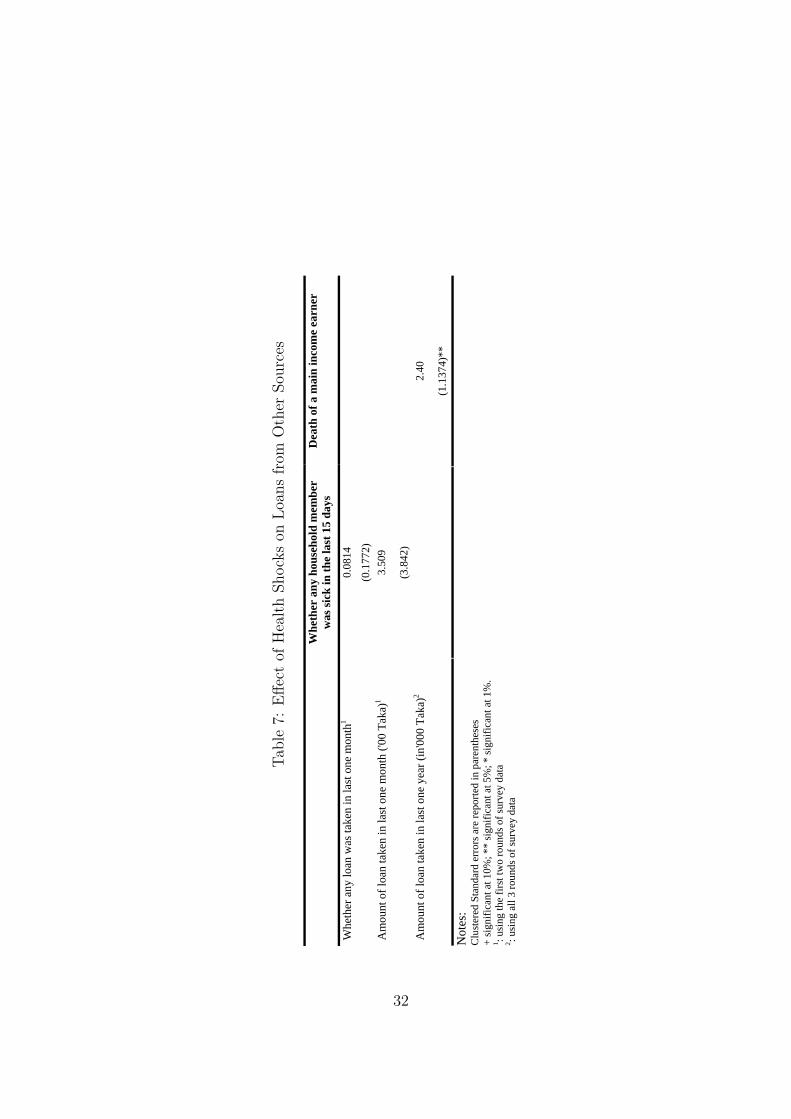
by borrowing from any other source. The estimated equation takes the following form:
Livt = α0 + α1Hivt + α2Xivt + δv + µt + (δv × µt) + εivt (9)
A positive and statistically significant estimate of α1 implies that a household responds to
a health shock by borrowing more from other sources.
We use three alternative measures of loans from other sources:
1. whether any loan was taken in the last one month (binary variable);
2. amount of loan taken in the last one month; and
3. amount of loan taken in the last one year
On the other hand we consider two health shock variables:
1. whether any member of the household has been sick in the last 15 days
2. whether the main household earner died in the last one year
The Fixed Effects Logit and the Random Effects Tobit regression results presented in Table
7 show that the death of the main earner in the household is associated with increased
borrowing in the last one year. This result indicates that long term health shocks increase
borrowing from other sources, such as relatives, friends or informal money lenders.
Households can also insure consumption by selling productive (for example livestock) or
non-productive (for example consumer durable) assets.14 Households that have access to
14The value of consumer durable is the aggregated current market value of items like radio, fans, boatsand pots that are owned by the household. The information on the stock of assets is available only at theyear level.
15

microcredit might have focused on its asset building and on the creation or expansion of
one or more income generating activities compared to households that do not. Similarly,
livestock is a very important asset in rural Bangladesh. A considerable portion of the
households in our sample save in the form of investment in livestock. Almost all the
households possess some livestock (e.g., cows, goats, chicken, ducks, etc.). There has been
a considerable attention paid by previous studies on the role of livestock as a buffer stock.15
To examine the issue of how purchase and sale of assets and livestock is used to smooth
consumption in response to health shocks, we estimate an equation similar to equation (7):
the only difference being that here the dependent variable is the change in the values of
assets owned by the household. The estimated equation is:
∆Aivt = β0 + β1Hivt + β2Xivt + β3(Hivt ×Divt) + δv + µt + (δv × µt) + εivt (10)
Here ∆Aivt measures the change in ownership of non-land asset or livestock over two suc-
cessive rounds of the survey. A negative and statistically significant β1 implies that the
household reduces its ownership of assets or livestock in response to a health shock. A pos-
itive and statistically significant β3 implies that access to microcredit reduces the impact
of the health shock and households do not need to take re-course to sale of assets to insure
against health shocks. The 2SLS and OLS fixed effects estimates of the mitigating effects
of microcredit on sale of assets and livestock are presented in Table 8. While the coefficient
estimates of β1 and β3 do not have a systematic pattern in the case of change in ownership
of non-productive assets, those for the change in ownership of livestock are much more
systematic. The coefficient estimate associated with the health shock variable is always
negative and generally statistically significant in the change in value of livestock regres-
sions. In addition, the difference estimate is generally positive and statistically significant
15Fafchamps, Udry, and Czukas (1998) find limited evidence that livestock inventory serve as bufferstock against large variation in crop income induced by severe rainfall shock. They find that livestocksales compensate for 15-30 percent of income shortfalls due to village level shock. On the other hand intheir study of consumption insurance and vulnerability in a set of developing and transitional countriesSkoufias and Quisumbing (2005) find that loss of livestock do not have a significant negative effect on thegrowth rate of consumption per-capita. Kazianga and Udry (2006) also find little evidence of the use oflivestock as buffer stocks for consumption smoothing. Instead they find households rely exclusively onself-insurance in the form of adjustments to grain stocks to smooth out consumption. Park (2006) findsthat households who do not live very close to other households do sell off their livestock and other assetswhen experience a shock.
16

implying that households with access to microcredit are less likely to sell livestock in order
to insure against health shocks. However the total effect is generally still negative (and
statistically significant), implying that even these households (with access to microcredit)
are not fully able to insure against health shocks and need to sell assets and livestock (in
particular) to insure consumption.
4.4 Income Smoothing and Consumption Smoothing
Next we estimate the extent to which households are able to insure consumption. This
magnitude is critical for assessing the importance of our findings for welfare and for consid-
ering their policy implications. Rather than directly examining the impact of microcredit,
here we examine the role of transitory changes in income on consumption smoothing. If
permanent income hypothesis model holds, then household would smooth consumption
when facing temporary income fluctuations. We measure the extent to which households
are not able to insure consumption against illness as the share of the costs of illness that
are financed out of consumption. To do so, we estimate a model of the effect of changes in
(net of medical spending) income on the growth of consumption. Specifically, we estimate
the following regression:
∆Civt = φ0 + γ∆Yivt + θXivt + δv + µt + (δv × µt) + εivt (11)
where Yivt is income minus medical care expenditure of household i in village v in year t.16
If there is perfect income insurance within a village, then changes in household income will
have no effect on consumption after controlling for common village and time effects, i.e., γ =
0. Income is however potentially endogenous because of the correlation of the error term
with the growth in income and consumption. It is also likely to be measured with error. So
we account both endogeneity and measurement error in income by instrumental variable
estimation of equation (11). We use the health shock variable as the relevant instrument
16Income includes earnings from self-employment and business activities, net wages earned, net profitsfrom crop and livestock production. It excludes net borrowing or savings and gifts received. It is to benoted that income is measured annually. So seasonal variation of income is not captured in our data.Some of the categories of income (such as income from household production and working in a householdenterprise) are imputed.
17

for changes in income under the assumption that changes in consumption due to changes in
income is due only to changes in income due to health shock. Table 9 presents the OLS and
2SLS results of the estimated coefficient γ. OLS estimates show that there is a significant
but very small relationship between income changes and consumption changes. A 100 Taka
increase in income is estimated to increase total (food and non-food) consumption by only
0.43 Taka. 2SLS coefficients are larger but are not statistically significant. This is possibly
due to the lack of sufficient variation in income changes in response to health shocks.17
The results essentially suggest that households are not fully able to smooth consumption
in response to transitory income shocks and transitory income shocks induced by health
shocks can have a long term effect on consumption. The coefficient estimates suggest
that a 100 Taka increase in income is estimated to increase food expenditure by 12 Taka.
The effects are much stronger for non-participants. A 100 Taka increase in income is
estimated to increase consumption expenditure by 38 taka for the control group, while it
does increase only by 1.3 Taka for the treatment group. Since health shocks reduces income,
a positive coefficient, albeit indirectly, indicates that health shocks have negative influence
on consumption smoothing and that the results are stronger for the control households.
4.5 Using Alternative Estimation Techniques
Our identification strategy is based on the implicit assumption of separability between con-
sumption and health status. Otherwise, health status would change the marginal utility of
consumption (see for example Gertler and Gruber (2002)). Therefore, α1 in equation (6)
might not be an unbiased estimator of the effect of idiosyncratic shock on changes in con-
sumption because health shock may be correlated with omitted preferences (error term),
biasing the estimated value of α1 in equation (6). There are some additional estimation
issues that need to be considered here. For example the perception of being sick or being
healthy can vary considerably across households. This could lead to a significant mea-
surement error problem. If measurement error is random, then we do not need to worry
17We use number of days sick in previous year as instrument for change in income. We also experimentwith other health shock variables using these as instruments for changes in income, but none of themcapture enough variation of changes in income − a result consistent with our earlier findings in regard tochanges in consumption
18

about this. However, it is possible that likelihood of reporting illness is closely related to
the socio-economic status of the household (for example the income of the household or
the education level of the most educated member of the family). Additionally, our sample
consists of households who have been exposed to the treatment and those who have not
been. If households in the treatment group have a better knowledge about how to prevent
sickness, or have better coping strategies because of training provided by the microcredit
providers then we could expect that either households in treatment group are system-
atically less exposed to shock or even when they experience such a shock we would not
observe significant changes in consumption because of the specific design of the microcredit
program.
We can indeed adopt an IV strategy here to control for time-varying unobserved hetero-
geneity affecting the changes in consumption and health shocks.18 For this, we need to
search for a variable that is correlated with health shock but does not directly affect the
changes in consumption expenditure and the variable is not correlated with idiosyncratic
error term. Remember that past health does not have any persistent or permanent effects
on current health. We cannot therefore use lagged health shock as instrument for current
health shock. We experimented with past family income/consumption/household charac-
teristics as the relevant instrument, but none of these appeared to be satisfactory. Lacking
an identifying instrument, we choose to adopt the propensity score matching (PSM) strat-
egy of Rosenbaum and Rubin (1983) that is now widely used in the program evaluation
literature.19 Typically we would expect that the likelihood of reporting illness is closely
related to individual/household characteristics. We therefore match households based on
their socio-economic status. We include a number of household characteristics and restrict
our analysis to the matched sample. This controls for heterogeneity in initial socioeconomic
conditions that may be correlated with subsequent health shocks and the path of consump-
18Unobserved heterogeneity that is time invariant in this context is automatically captured by ourregression specification. The vector X in the regression controls for observed heterogeneity.
19In our case, PSM compares households who reported illness to those that did not, with the same(or similar) values of those variables thought to influence both illness and consumption. We can thinkhouseholds reporting illness in our sample as treatment group and the households that did not as the controlgroup, following the program evaluation literature. Under the matching assumption, the only remainingdifference between the two groups is reported sickness. Any difference in outcome between these two groupscan be entirely attributed to the sickness effect provided we are able to have made sufficient arguments toguarantee that there are no further systematic differences between these two groups.
19

tion growth. To estimate the propensity score we estimate a conditional fixed-effects logit
model with binary dependent variable whether a member of household was reported to
be sick (=1) or not (= 0) using the panel data. So, unlike a cross-sectional propensity
score estimate, we control for unobservables that might influence households reporting of
sickness. We then discard observations that do not have any common support, and obser-
vations with households having very low or very high probability of sickness. We consider
a caliper matching method, which uses all of the comparison units within a predefined
propensity score radius. Therefore, we use only as many comparison units as are available
within the calipers, allowing for the use of extra (fewer) units when good matches are (not)
available (Dehejia and Wahba, 2002). We set the radius less than or equal to 0.00005, and
discard about one-third of the observations from the sample (these do not have common
support within this propensity score range). We combine matching with IV approach (to
account for measurement error) to estimate the effects of health shocks and the role of
microcredit in mitigating the consequences of health shocks. The results are reported in
Table 10. The sign of the estimated coefficients are similar to that of 2SLS estimates using
the full sample. The magnitude of the health shocks coefficients are, in general, larger using
matched sample. The interaction terms of loan and health shock variables also indicate
a larger coefficient estimates and most of them are statistically significant. Our results
are again indicative of the role of microcredit in insuring households against idiosyncratic
health shocks.
5 Conclusion
This paper examines, using a large panel data set from Bangladesh, the ability or otherwise
of poor households to insure against idiosyncratic and unanticipated health shocks. Also,
we assess the role of microcredit. Our results suggest that even though consumption
remains stable in many cases when households are exposed to health shocks, households
that have access to microcredit appear to cope (slightly) better. The most important
instrument used by households appear be sales of productive assets (livestock). There is a
significant mitigating effect of microcredit: households that have access to microcredit do
20

not need to sell livestock to the extent households that do not have access to microcredit
need to, in order to insure consumption against health shocks. The results therefore suggest
that microcredit organizations and microcredit per se have an insurance role to play, an
aspect that has not been analyzed previously. The welfare implications of microcredit
therefore remain high.
21

References
Amin, S., A. Rai, and G. Topa (2003): “Does microcredit reach the poor and vulner-
able? Evidence from northern Bangladesh,” Journal of Development Economics, 70(1),
59 – 82.
Asfaw, A., and J. Braun (2004): “Is Consumption Insured against Illness? Evidence on
Vulnerability of Households to Health Shocks in Rural Ethiopia,” Economic Development
and Cultural Change, 53, 115 – 129.
Beegle, K., J. D. Weerdt, and S. Dercon (2008): “Adult mortality and consumption
growth in the age of HIV/AIDS,” Economic Development and Cultural Change, 56, 299
– 326.
Besley, T. (1995): “Nonmarket Institutions for Credit and Risk Sharing in Low-Income
Countries,” Journal of Economic Perspectives, 9(3), 115 – 127.
Cochrane, J. H. (1991): “A Simple Test for Consumption Insurance,” Journal of Polit-
ical Economy, 99(5), 957 – 976.
Dehejia, R., and S. Wahba (2002): “Propensity Score Matching Methods for Non-
Experimental Causal Studies,” Review of Economics and Statistics, 84, 151 – 161.
Dercon, S., and P. Krishnan (2000): “In Sickness and in Health: Risk Sharing within
Households in Rural Ethiopia,” Journal of Political Economy, 108(4), 688 – 727.
Fafchamps, M., C. Udry, and K. Czukas (1998): “Drought and Saving in West
Africa: Are Livestock a Buffer Stock?,” Journal of Development Economics, 55(2), 273
– 305.
Gertler, P., and J. Gruber (2002): “Insuring Consumption Against Illness,” American
Economic Review, 92(1), 51 – 76.
Jalan, J., and M. Ravallion (1999): “Are the Poor Less Well Insured? Evidence
on Vulnerability to Income Risk in Rural China,” Journal of Development Economics,
58(1), 61 – 81.
22

Kazianga, H., and C. Udry (2006): “Consumption Smoothing? Livestock, Insurance
and Drought in Rural Burkina Faso,” Journal of Development Economics, 79(2), 413 –
446.
Kochar, A. (1995): “Explaining Household Vulnerability to Idiosyncratic Income
Shocks,” American Economic Review, 85(2), 159 – 164.
Lindelow, M., and A. Wagstaff (2007): “Health shocks in China: are the poor
and uninsured less protected?,” Discussion paper, Policy Research Working Paper 3740,
World Bank.
Morduch, J. (1995): “Income Smoothing and Consumption Smoothing,” Journal of
Economic Perspectives, 9(3), p103 – 114.
Morduch, J. (1999): “Between the Market and State: Can Informal Insurance Patch the
Safety Net?,” World Bank Research Observer, 14(2), 212 – 223.
Park, C. S. (2006): “Risk Pooling Between Households and Risk Coping Measures in
Developing Countries: Evidence from Rural Bangladesh,” Economic Development and
Cultural Change, 54(2), 423 – 457.
Pitt, M. M., and S. R. Khandker (1998): “The Impact of Group-Based Credit Pro-
grams on Poor Households in Bangladesh: Does the Gender of Participants Matter?,”
Journal of Political Economy, 106(5), 958 – 996.
(2002): “Credit Programmes for the Poor and Seasonality in Rural Bangladesh,”
Journal of Development Studies, 39(2), 1 – 24.
Ravallion, M., and S. Chaudhuri (1997): “Risk and Insurance in Village India: Com-
ment,” Econometrica, 65(1), 171 – 184.
Rosenbaum, P., and D. Rubin (1983): “The Central Role of the Propensity Score in
Observational Studies for Causal Effects,” Biometrika, 70(1), 41 – 55.
Rosenzweig, M. R., and K. I. Wolpin (1993): “Credit Market Constraints, Consump-
tion Smoothing, and the Accumulation of Durable Production Assets in Low-Income
23

Countries: Investment in Bullocks in India,” Journal of Political Economy, 101(2), p223
– 244.
Schultz, T. P., and A. Tansel (1997): “Wage and Labor Supply Effects of Illness in
Cote D’Ivoire and Ghana: Instrumental Variable Estimates for Days Disabled,” Journal
of Development Economics, 53(2), 251 – 286.
Skoufias, E., and A. Quisumbing (2005): “Consumption Insurance and Vulnerability
to Poverty: A Synthesis of the Evidence from Bangladesh, Ethiopia, Mali, Mexico and
Russia,” The European Journal of Development Research, 17(1), 24–58.
Townsend, R. M. (1994): “Risk and Insurance in Village India,” Econometrica, 62(3),
539 – 591.
Udry, C. (1990): “Credit Markets in Northern Nigeria: Credit as Insurance in a Rural
Economy,” World Bank Economic Review, 4(3), 251 – 269.
Wagstaff, A. (2007): “The Economic Consequences of Health Shocks: Evidence from
Vietnam,” Journal of Health Economics, 26(1), 82 – 100.
24

Tab
le1:
Hou
sehol
dL
evel
Des
crip
tive
Sta
tist
ics
19
97-1
998
19
99-2
000
20
04-2
005
Mea
n St
d.
Dev
iatio
n M
ean
Std.
D
evia
tion
Mea
n St
d.
Dev
iatio
n Pa
nel A
: Hea
lth S
hock
Var
iabl
es
Whe
ther
any
mem
ber w
as si
ck in
last
15
days
0.
492
0.50
0 0.
438
0.49
6 0.
211
0.40
8 N
umbe
r of d
ays s
ick
in la
st 1
5 da
ys d
ue to
sick
ness
2.
445
3.18
7 2.
056
2.93
0 1.
306
3.06
5 N
umbe
r of d
ays w
ork
lost
due
to si
ckne
ss
3.11
9 3.
631
3.01
7 3.
095
1.34
9 3.
057
Whe
ther
hou
seho
ld in
curr
ed a
ny b
ig e
xpen
ditu
re
0.15
7 0.
402
0.14
4 0.
352
0.22
6 0.
419
Dea
th o
f the
mai
n ea
rner
in th
e fa
mily
0.
010
0.01
2 0.
010
0.10
1 0.
015
0.12
1 Pa
nel B
: Dem
ogra
phic
Var
iabl
es
Age
of t
he H
ouse
hold
Hea
d 44
.52
13.3
6 46
.81
13.3
4 47
.75
12.2
0 N
umbe
r of w
orki
ng p
eopl
e in
the
hous
ehol
d 2.
81
1.38
3.
02
1.53
3.
59
2.12
H
ouse
hold
size
5.
63
2.29
6.
06
2.48
7.
23
3.85
M
axim
um e
duca
tion
atta
ined
by
any
hous
ehol
d m
embe
r 5.
48
4.13
6.
23
4.07
7.
27
6.53
A
rea
of a
rabl
e la
nd
68.4
7 14
6.66
80
.79
159.
03
73.6
8 22
5.92
N
umbe
r of c
hild
ren
2.83
1.
66
2.22
1.
46
3.01
2.
39
Num
ber o
f wom
en
2.66
1.
40
2.94
1.
52
3.26
2.
00
Num
ber o
f old
peo
ple
of a
ge 6
0 ab
ove
0.25
0.
49
0.39
0.
60
0.31
0.
54
Num
ber o
f mar
ried
peop
le
2.38
1.
10
2.70
1.
37
3.16
1.
98
Whe
ther
wom
en is
the
head
of t
he h
ouse
hold
0.
05
0.23
0.
05
0.23
0.
11
0.31
25

Tab
le1
(con
tinued
):H
ouse
hol
dL
evel
Des
crip
tive
Sta
tist
ics
Pane
l C: O
utco
me
Var
iabl
e (in
Tak
a)
Food
Con
sum
ptio
n (M
onth
ly)
2432
.8
1832
.2
2949
.5
2721
.1
3214
.4
3296
.1
Non
-Foo
d co
nsum
ptio
n ex
pend
iture
(yea
rly)
5628
.2
6877
.2
3499
.4
7022
.8
6024
.0
9563
.7
Non
-land
Ass
et (e
xclu
ding
live
stoc
k)
1312
8.1
2732
7.5
1852
9.7
1455
4.0
1766
1.2
4439
4.1
Val
ue o
f liv
esto
ck
5956
.2
7664
.7
4027
.5
6242
.8
4296
.7
7432
.9
Inco
me
3297
5.1
3357
2.6
3573
3.6
5080
4.0
4525
2.5
5051
5.5
Self-
empl
oym
ent i
ncom
e 60
09.8
10
4059
.0
5377
.4
2884
2.5
6788
.1
6398
7.5
Med
ical
Exp
endi
ture
21
91.5
10
254.
5 20
15.7
87
99.6
42
95.1
12
406.
1 To
tal n
on-f
ood
incl
udin
g m
edic
al e
xp (m
onth
ly)
651.
6 14
27.6
45
9.6
1318
.5
859.
9 18
30.8
To
tal e
xpen
ditu
re
3084
.5
3259
.9
3409
.0
4039
.7
4074
.3
5126
.9
Perc
enta
ge o
f non
-foo
d in
tota
l exp
endi
ture
21
.1
13
.5
21
.1
N
umbe
r of o
bser
vatio
ns
2694
2694
2694
26

Tab
le2:
Des
crip
tive
Sta
tist
ics.
Mic
rocr
edit
and
Oth
erL
oans
(in
Tak
a)
19
97-1
998
19
99-2
000
20
04-2
005
Mea
n St
d.
Dev
iatio
n M
ean
Std.
D
evia
tion
Mea
n St
d.
Dev
iatio
n M
icro
redi
t bor
row
ing
Am
ount
of l
oan
take
n fr
om M
icro
cred
it or
gani
zatio
n 74
27.3
71
65.0
10
616.
8 11
332.
4 11
682.
5 17
378.
7 N
umbe
r of m
icro
cred
it bo
rrow
ers
1592
1532
1280
Bor
row
ing
from
oth
er so
urce
s
Pe
rcen
tage
of h
ouse
hold
s tak
en lo
an in
last
mon
th
5.18
4.3
N
A
A
mou
nt o
f loa
n ta
ken
in la
st m
onth
16
7 22
84.1
46
8.07
15
573.
2
Pe
rcen
tage
of h
ouse
hold
s tak
en lo
an in
last
yea
r 29
.4
26
.6
18
Am
ount
of l
oan
take
n in
last
yea
r 46
57.2
12
712.
1 73
50.7
28
640.
3 94
64.0
18
045.
8 Pe
rcen
tage
of h
ouse
hold
s who
took
loan
from
nei
ghbo
ur a
nd
rela
tives
53
35.1
NA
Perc
enta
ge o
f hou
seho
lds w
ho to
ok lo
an fo
r con
sum
ptio
n 23
.4
11
.1
9.
1
Perc
enta
ge o
f hou
seho
lds w
ho to
ok lo
an fo
r med
ical
pur
pose
3.
5
0.5
0.
6
Not
e: M
onth
ly lo
an d
ata
is n
ot a
vaila
ble
for t
he la
st ro
und
of su
rvey
200
4-05
27

Table 3: Persistence of Health Shock. Coefficient Corresponding to the Lag Health ShockVariable
Fixed effects IV1 IV2 -0.193 0.1 0.005 Whether any household member is sick in
period t-1 (6.78) (0.266) (0.127) Whether incurred any big expenditure 0.002 3.543 -0.169 or income loss due to sickness in period t-1 (0.003) (14.081) (0.453)
-0.016 1.106 -0.12 Death of the main family member in period t-1
(0.023) (2.145) (0.162)
Notes: Clustered Standard errors are reported in parentheses IV1 includes only two period lagged value of the dependent variable as instrument, IV2 adds household level characteristics of two period-lag as instruments
28

Tab
le4:
Eff
ect
ofH
ealt
hShock
son
Chan
ges
inC
onsu
mpti
on
Dep
ende
nt V
aria
ble
Cha
nge
in F
ood
Con
sum
ptio
n C
hang
e in
Non
-foo
d C
onsu
mpt
ion
Shoc
k va
riab
le (p
ast 3
0 da
ys)
Whe
ther
any
hou
seho
ld m
embe
r is
sick
12.
475
2.45
8 1.
728
1.93
2
(1
.785
) (1
.848
) (1
.770
) (1
.21)
Num
ber o
f day
s sic
k
3.36
4 2.
759
3.01
2 0.
272
(2
.059
) (2
.018
) (2
.057
) (2
.202
)
Num
ber o
f Wor
king
day
s los
t -1
.61
-2.6
88
-2.6
88
-3.4
86
(2
.144
) (2
.351
) (2
.351
) (2
.158
)
Sh
ock
vari
able
( pa
st o
ne y
ear)
-3
.417
-0
.367
-0
.335
0.
0188
2.
69
2.54
1.
99
1.05
W
heth
er h
ouse
hold
incu
rred
any
big
ex
pend
iture
or i
ncom
e lo
ss d
ue to
si
ckne
ss1
(1.9
57)+
(0
.209
)+
(0.1
97)+
(0
.121
) ‘(
0.63
5)*
(0.6
94)*
(0
.658
)*
(0.6
49)
D
eath
of t
he m
ain
fam
ily e
arne
r1-1
.61
-0.5
5 -0
.409
0.
312
2.54
2.
96
2.73
1.
64
(2
.144
) (0
.431
) (0
.425
) (0
.252
) ‘(
1.25
9)**
(1
.306
)**
(1.2
36)*
* (1
.316
) V
illag
e Fi
xed
effe
cts
No
yes
yes
yes
No
yes
yes
yes
Tim
e Ef
fect
s N
o N
o ye
s ye
s N
o N
o ye
s ye
s V
illag
e*tim
e FE
N
o N
o N
o ye
s N
o N
o N
o ye
s
Not
es:
Clu
ster
ed S
tand
ard
erro
rs in
par
enth
eses
; +
sign
ifica
nt a
t 10%
; **
sign
ifica
nt a
t 5%
; * si
gnifi
cant
at 1
%.
1 : coe
ffic
ient
s are
div
ided
by
100
for c
hang
es in
food
con
sum
ptio
n, d
ivid
ed b
y 10
00 fo
r cha
nges
in n
on-f
ood
cons
umpt
ion
29

Tab
le5:
Eff
ect
ofH
ealt
hShock
son
Chan
ges
inC
onsu
mpti
onan
dth
eM
itig
atin
gE
ffec
tsof
Mic
rocr
edit
Dep
ende
nt V
aria
ble
Cha
nge
in F
ood
Con
sum
ptio
n C
hang
e in
Non
-foo
d C
onsu
mpt
ion
1.75
8 1.
786
0.87
5 0.
108
Whe
ther
any
hou
seho
ld m
embe
r is s
ick1
(1.8
84)
(1.9
55)
(1.9
52)
(1.5
11)
Shoc
k *
Trea
tmen
t 1.
3 1.
211
1.37
8 1.
392
(0
.05)
**
(0.5
322)
**
(0.5
28)*
* (0
.985
3)
Num
ber o
f day
s sic
k
2.4
1.66
3 1.
842
-0.8
68
(2
.340
) (2
.238
) (2
.281
) (2
.526
)
Sh
ock
* Tr
eatm
ent
0.00
58
0.00
66
0.00
70
0.00
69
(0
.003
9)
(0.0
038)
+ (0
.004
1)+
(0.0
065)
-2
.489
-3
.411
-3
.682
-4
.775
N
umbe
r of W
orki
ng d
ays l
ost
(2.1
75)
(2.3
71)
(2.3
39)
(2.1
45)*
*
Sh
ock
* Tr
eatm
ent
0.02
13
0.01
76
0.02
36
0.03
16
(0
.022
9)
(0.0
245)
(0
.023
4)
(0.0
214)
-0.3
55
-0.3
68
-0.3
44
-0.0
65
2.48
9 2.
36
2.36
1.
18
Whe
ther
hou
seho
ld in
curr
ed a
ny b
ig
expe
nditu
re o
r inc
ome
loss
due
to
sick
ness
1(0
.202
)+
(0.2
12)+
(0
.202
)+
(0.1
27)
(0.6
75)*
(0
.736
)*
(0.7
36)*
(0
.676
)+
Shoc
k *
Trea
tmen
t 0.
159
0.09
7 0.
106
0.86
9 2.
27
2.1
.947
4 -1
.411
(0.3
56)
(0.4
03)
(0.4
05)
(0.7
83)
(1.5
54)
(1.7
0)
(2.4
46)
(2.3
77)
Dea
th o
f the
mai
n fa
mily
ear
ner 1
-1.8
15
-1.7
264
-1.6
28
0.77
8 2.
605
2.62
2.
46
1.49
(4
.213
) (4
.423
) (4
.423
) (2
.869
) (1
.342
)+
(1.3
64)+
(1
.364
)+
(1.4
29)
Shoc
k *
Trea
tmen
t 1.
46
1.15
1.
195
2.32
-0
.065
9 3.
3 2.
595
1.4
(9
.030
) (1
8.75
) (1
8.57
) (1
1.79
) (3
.914
) (2
.80)
(2
.632
) (2
.70)
V
illag
e Fi
xed
effe
cts
No
yes
yes
yes
No
yes
yes
yes
Tim
e Ef
fect
s N
o N
o ye
s ye
s N
o N
o ye
s ye
s V
illag
e*tim
e FE
N
o N
o N
o ye
s N
o N
o N
o ye
s
Not
es:
Clu
ster
ed S
tand
ard
erro
rs in
par
enth
eses
; + si
gnifi
cant
at 1
0%; *
* si
gnifi
cant
at 5
%; *
sign
ifica
nt a
t 1%
. Tr
eatm
ent c
oeff
icie
nts a
re m
ultip
lied
by 1
00.
1 : coe
ffic
ient
s are
div
ided
by
100
for c
hang
es in
food
con
sum
ptio
n, d
ivid
ed b
y 10
00 fo
r cha
nges
in n
on-f
ood
cons
umpt
ion
30

Table 6: 2SLS Estimates of the Effect of Health Shocks on Changes in Consumption andthe Mitigating Effects of Microcredit
Dependent Variable Change in
Food Expenditure Non-Food Expenditure
-2.32 Whether any household member is sick1
(2.65)
Shock * Treatment 14.2
(16.1)
Number of days sick1 -0.086
(0.132)
Shock * Treatment 0.51
(0.79)
Number of Working days lost1 -0.259
(25.97)
Shock * Treatment 0.554
(0.638)
-1.43 -15.49 Whether household incurred any big expenditure or income loss due to sickness2
(1.77) (18.26)
Shock * Treatment 18.4 209.4
(22.7) (231.3)
Death of the main family earner2 -3.67 -40.66
(4.48) (37.94)
Shock * Treatment 39.4 418.2
(44.2) (373.7)
Notes Each set of coefficients is obtained from a separate regression of changes in outcome variable on health shock variables (left side of the table) and their interaction with instrumented loan variable. Each regression also incorporates village fixed effects, time effects and their interactions. Shock * Treatment coefficients are multiplied by 100. 1: coefficients are divided by 100 2: coefficients are divided by 1000 for changes in non-food consumption
31
Tab
le7:
Eff
ect
ofH
ealt
hShock
son
Loa
ns
from
Oth
erSou
rces
W
heth
er a
ny h
ouse
hold
mem
ber
was
sick
in th
e la
st 1
5 da
ys
Dea
th o
f a m
ain
inco
me
earn
er
0.08
14
W
heth
er a
ny lo
an w
as ta
ken
in la
st o
ne m
onth
1 (0
.177
2)
3.
509
A
mou
nt o
f loa
n ta
ken
in la
st o
ne m
onth
('00
Tak
a)1
(3.8
42)
2.40
A
mou
nt o
f loa
n ta
ken
in la
st o
ne y
ear (
in'0
00 T
aka)
2
(1
.137
4)**
Not
es:
Clu
ster
ed S
tand
ard
erro
rs a
re re
porte
d in
par
enth
eses
+
sign
ifica
nt a
t 10%
; **
sign
ifica
nt a
t 5%
; * si
gnifi
cant
at 1
%.
1 : usi
ng th
e fir
st tw
o ro
unds
of s
urve
y da
ta
2 : usi
ng a
ll 3
roun
ds o
f sur
vey
data
32

Table 8: Effect of Health Shocks on Change in Ownership of Assets and Livestock Change in Assets Change in Livestock
OLS 2SLS OLS 2SLS
0.0501 -7.94 Whether any household member is sick in the last 15 days (0.2217) (4.657)+
Shock * Treatment -0.12 129.7
(1.38) (75.4)+
Number of days sick 0.0038 -0.7878
(0.0082) (0.8989)
Shock * Treatment 0.0317 4.79
(0.01)* (5.4)
Number of Working days lost -0.0014 -2.207
(0.0042) ‘(1.271)+
Shock * Treatment 0.029 5.4
(0.03) (3.1)+
3.013 -11.58 -193.87 -15.20 Whether household incurred any big expenditure or income loss due to sickness (1.233)** (22.562) (229.19) (12.241)
Shock * Treatment 5.45 208.5 0.588 191.1
(6.68) (303.16) (0.707) ‘(155.2)
Death of the main family earner
-2.472 -46.80 -1.837 -38.59
(2.675) (52.66) (0.576) (18.86)**
Shock * Treatment -29.3 408.7 -0.91 362.7
(11.95)** (519.0) (2.92) (186.0)+
Notes: Clustered Standard errors are reported in parentheses + significant at 10%; ** significant at 5%; * significant at 1%. Regressions include Village Fixed Effects, Time Effects and Village * Time Fixed Effects Shock * Treatment coefficients are multiplied by 100.
33
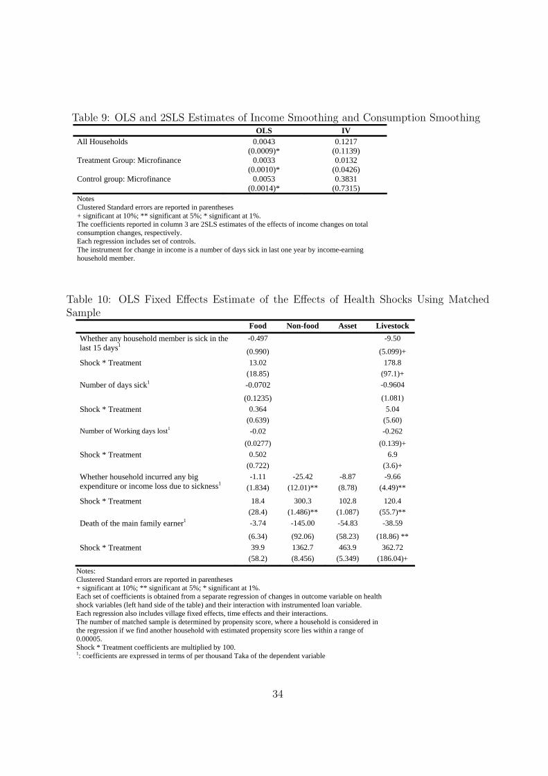
Table 9: OLS and 2SLS Estimates of Income Smoothing and Consumption Smoothing OLS IV All Households 0.0043 0.1217 (0.0009)* (0.1139) Treatment Group: Microfinance 0.0033 0.0132 (0.0010)* (0.0426) Control group: Microfinance 0.0053 0.3831 (0.0014)* (0.7315) Notes Clustered Standard errors are reported in parentheses + significant at 10%; ** significant at 5%; * significant at 1%. The coefficients reported in column 3 are 2SLS estimates of the effects of income changes on total consumption changes, respectively. Each regression includes set of controls. The instrument for change in income is a number of days sick in last one year by income-earning household member.
Table 10: OLS Fixed Effects Estimate of the Effects of Health Shocks Using MatchedSample
Food Non-food Asset Livestock -0.497 -9.50 Whether any household member is sick in the
last 15 days1(0.990) (5.099)+
Shock * Treatment 13.02 178.8 (18.85) (97.1)+ Number of days sick1 -0.0702 -0.9604
(0.1235) (1.081) Shock * Treatment 0.364 5.04 (0.639) (5.60) Number of Working days lost1 -0.02 -0.262 (0.0277) (0.139)+ Shock * Treatment 0.502 6.9 (0.722) (3.6)+
-1.11 -25.42 -8.87 -9.66 Whether household incurred any big expenditure or income loss due to sickness1
(1.834) (12.01)** (8.78) (4.49)**
Shock * Treatment 18.4 300.3 102.8 120.4 (28.4) (1.486)** (1.087) (55.7)** Death of the main family earner1 -3.74 -145.00 -54.83 -38.59
(6.34) (92.06) (58.23) (18.86) ** Shock * Treatment 39.9 1362.7 463.9 362.72 (58.2) (8.456) (5.349) (186.04)+
Notes: Clustered Standard errors are reported in parentheses + significant at 10%; ** significant at 5%; * significant at 1%. Each set of coefficients is obtained from a separate regression of changes in outcome variable on health shock variables (left hand side of the table) and their interaction with instrumented loan variable. Each regression also includes village fixed effects, time effects and their interactions. The number of matched sample is determined by propensity score, where a household is considered in the regression if we find another household with estimated propensity score lies within a range of 0.00005. Shock * Treatment coefficients are multiplied by 100. 1: coefficients are expressed in terms of per thousand Taka of the dependent variable
34