hayek, local information, and the decentralization …documents.worldbank.org/curated/en/... ·...
TRANSCRIPT
Policy Research Working Paper 7321
Hayek, Local Information, and the Decentralization of State-Owned Enterprises in China
Zhangkai Huang Lixing Li
Guangrong Ma Lixin Colin Xu
Development Research GroupFinance and Private Sector Development TeamJune 2015
WPS7321P
ublic
Dis
clos
ure
Aut
horiz
edP
ublic
Dis
clos
ure
Aut
horiz
edP
ublic
Dis
clos
ure
Aut
horiz
edP
ublic
Dis
clos
ure
Aut
horiz
ed
Produced by the Research Support Team
Abstract
The Policy Research Working Paper Series disseminates the findings of work in progress to encourage the exchange of ideas about development issues. An objective of the series is to get the findings out quickly, even if the presentations are less than fully polished. The papers carry the names of the authors and should be cited accordingly. The findings, interpretations, and conclusions expressed in this paper are entirely those of the authors. They do not necessarily represent the views of the International Bank for Reconstruction and Development/World Bank and its affiliated organizations, or those of the Executive Directors of the World Bank or the governments they represent.
Policy Research Working Paper 7321
This paper is a product of the Finance and Private Sector Development Team, Development Research Group. It is part of a larger effort by the World Bank to provide open access to its research and make a contribution to development policy discussions around the world. Policy Research Working Papers are also posted on the Web at http://econ.worldbank.org. The authors may be contacted at [email protected].
Hayek argues that local knowledge is a key for understand-ing whether production should be decentralized. This paper tests Hayek’s predictions by examining the causes of the Chinese government’s decision to decentralize state-owned enterprises. Since the government located closer to a state-owned enterprise has more information over that enterprise, a greater distance between the government and
the enterprise should lead to a higher likelihood of decen-tralization. Moreover, where communication costs and the government’s uncertainty over an enterprise’s performance are greater, the government is more likely to decentralize enterprises so that it can better utilize local information. This paper finds empirical support for these implications.

Hayek, Local Information, and the Decentralization of
State-Owned Enterprises in China1
Zhangkai Huang
Lixing Li
Guangrong Ma
Lixin Colin Xu
Keywords: Local information; organizational structure; decentralization; distance.
JEL codes: D23, D83, L22, L23, P20, P31
1 We have benefited from useful comments and help of Jens Matthias Arnold, Wouter Dessein, Price Fishback, Bert Hoffman, Sebestian Galiani, Gary Gorton, Hanan Jacoby, Beata S. Javorcik, Mathew Kahn, Gary Libecap, Cheryl Long, Bill Megginson, Peter Murrell, Mary Shirley, John Wallis, Shang-Jin Wei, Xiaobo Zhang and participants of the 15th NBER-CCER conference. Financial support from the National Natural Science Foundation of China (#71203004) is gratefully acknowledged. Author information. Zhangkai Huang: Tsinghua University, [email protected]. Lixing Li: CCER, Peking University, [email protected]. Guangrong Ma: Remin University, [email protected]. Lixin Colin Xu (corresponding author): World Bank, the Research Group, 1818 H Street, N.W., Washington, DC 20433; [email protected]; phone, 202 473 4664; fax, 202 522 1155.

2
“If we can agree that the economic problem of society is mainly one of rapid
adaptation to changes in the particular circumstances of time and space, it would
seem to follow that the ultimate decisions must be left to the people who are familiar
with these circumstances, who know directly of the relevant changes and of the
sources immediately available to meet them. We cannot expect that this problem
will be solved by first communicating all this knowledge to a central board, which,
after integrating all knowledge, issues its orders. We must solve it by some form of
decentralization.”
——— Hayek (1945)
1. Introduction
One of the most important economic dramas in the last century was the emergence
and then the decline of planned economy and state ownership. For more than half
a century, it seemed that socialism could be as productive, if not more, than
capitalist economy. In the 1973 edition of the economics textbook (Samuelson
1973), for instance, Samuelson predicted that the Soviet Union’s income level
would probably match that of the United States by 1990 and overtake it by 2010.
The debate of the merits of market socialism in the first half of the last century thus
involved top economists such as Oscar Lange, Abba Lerner, Ludwig von Mises,
and Frederick Hayek. The key arguments for why capitalism would be more
efficient than socialism are perhaps two: the stronger individual incentives under
the stronger protection of private property rights, and the efficiency of utilizing
specific information dispersed among individuals and plants (Boettke, 2004). The
second point is of course originated from Hayek (1945), one of the most influential
papers of all time.2 The key importance of incentives, ownership and property
2 As of April 2015, Hayek (1945) has been cited more than 12,000 times in Google Scholar, and it is viewed as one of the top 20 articles published in AER in its first 100 years’ history (Arrow et al. 2011).
3
rights for explaining performance in socialist and transitional economies is perhaps
one of the most active areas for research in the past few decades (Shleifer and
Vishny, 1994; Megginson and Netter 2001; Djankov and Murrell 2002; Acemoglu,
Johnson and Robinson 2001; Estrin et al., 2009). However, the importance of local
information for efficiency in socialist or transitional economies or the state-owned
sector is rarely systematically empirically explored.
In this paper we examine the causes of decentralizing state-owned
enterprises (SOEs) in China, focusing on the role of local information. The data we
use is the Annual Survey of Industrial Firms (ASIF) 1998-2007, which covers non-
state firms with sales exceeding 5 million yuan and all SOEs. Decentralization
here is defined as the oversight government of an SOE shifting from a higher to a
lower level of government—that is, from the central to provincial, or from
provincial to municipality (alternatively called prefecture), or from municipality to
county government. 3 The availability of local information is captured by the
distance between an SOE and its oversight government. A larger distance between
the oversight government and the SOE implies that the oversight government can
have less direct observations on firm performance, managerial competence, and
firm competitiveness. Indeed, there is a large literature providing evidence that
distance has huge consequences for firms. For instance, distance (in terms of trust
level and physical distance) helps explain decentralization decision between
multinational headquarters and oversea subsidiaries (Bloom, Sadun and Van
Reenen, 2012); distance helps explain a headquarters’ investment allocation across
plants in different locations (Giroud 2013); distance has been found to have
profound implications for the lending relationship between banks and firms
(Peterson and Rajan 1994, 2002; Mian, 2006; Agarwal and Hauswalkd, 2010); and
3 Chinese local government consists of several (from higher to lower) levels as follows: province, municipality (or prefecture), county, and township. As of 1998, there are 31 provincial-level, 331 municipal-level, and 2863 county-level governments.

4
distance has been found to be a good proxy of information asymmetry in financial
markets (Coval and Moskowitz 1999; Garmaise and Moskowitz, 2004; Grinblatt
and Keloharju 2001; Hau, 2001).
Hayek (1945) implies that it would be more efficient for the oversight
government with a larger distance to the SOE to delegate (or decentralize) the
control rights to a lower level of government, which in general has a shorter
distance to the SOE. Moreover, when firms’ performance is harder to predict—and
therefore local information figures more prominently—the same distance implies a
stronger tendency to decentralize so as to better utilize local information. In
addition, when communication costs are lower, the oversight government has less
difficulty finding out what is going on in the SOE, and the same distance then
implies a weaker tendency to decentralize. We should point out here that Hayek’s
point does not imply that SOEs should always be decentralized so that the distance
between the SOE and the oversight government should be minimal. Tilting the
balance toward centralizing include other considerations, such as internalizing
externality of the SOE, pursuing goals of upper levels of government, and making
top-notch experts who can specialize in complex and difficult problems to be in
charge of some sophisticated SOEs (Garicano 2000).
We find support for these conjectures implied by Hayek (1945). In
particular, the larger the distance between the oversight government and the SOE,
the more likely the oversight government is to decentralize the SOE. Moreover, the
positive decentralization-distance link is stronger when firm performance exhibits
more uncertainty, and when communication costs are higher (as proxied by lower
density of road, telecom or internet).
The relationship between decentralization and distance may be subject to
other interpretations. To ensure that our interpretation is the right one, we conduct
a number of checks. We mitigate omitted variable bias by including industry and
year fixed effects, dummies indicating the same original oversight government,

5
along with province-year-level macro controls (and in an alternative specification,
fiscal conditions of the original oversight government and its lower level
government). To guard against the possibility that the distance to the oversight
governments may be simply a proxy for the distance to agglomeration centers, we
construct a placebo distance to an alternative agglomeration city (at the same level
as the oversight government), and this placebo distance measure is not significantly
related to decentralization. Finally, we rely on exogenous source of variation of
distance to identify its effect on decentralization. In particular, in the 1960s and
1970s, a large number of SOEs were relocated to inland provinces to confront the
possibility of external wars with the Soviet Union and the U.S. As a result, their
distance to their oversight governments was determined historically and likely had
nothing to do with the decentralization decisions decades later. The instrumental
variable results are qualitatively similar to our base specification.
To the best of our knowledge, this paper is the first paper that tests Hayek’s
idea of the fundamental importance of local information for understanding the
workings of the economic system, in particular, the centralization or
decentralization of state-owned enterprises. We test rich implications of Hayek’s
idea, such as how decentralization depends on the distance to the oversight distance
government, and how this link depends on firm heterogeneity and communications
costs.
Our paper is most closely related to the empirical literature examining
decentralization within firms. In particular, Aghion et al. (2007) provide evidence
that the availability of public information to the headquarters reduces the need to
delegate controls to the manager. Bloom et al. (2009) provide evidence that
information technology and communication technology have different implications
for within-firm decentralization, with the former facilitating, while the latter
hindering, decentralization. Bloom, Sadun and Van Reenen (2010, 2012) find that
competition and trust foster greater decentralization. Giroud (2013), perhaps the

6
only paper that examines how the within-firm distance between headquarters and
their plants affects plant performance, find that proximity of the headquarters to a
plant significantly increases the plant’s investment and productivity. We differ from
these papers in two ways. First, we focus on the role of distance between the
oversight government and an SOE in the state sector for the decentralization
decision of SOEs, and therefore directly address the original concern of Hayek in
understanding the role of local information in determining efficiency of
centralization versus decentralization. Second, the nature of our data set allows us
to explore changes in organizational structure, thus we study decentralization in a
dynamic setting. Our findings thus are complementary to the literature on
decentralization within an organization—here we view the whole state economy of
China as a gigantic organization with the state as the ultimate owner—that
emphasizes the role of information in determining the control rights structure. We
offer empirical support for the insight of the critical importance of local information
in shaping the organization structure in the largest “organization” (i.e., the state
economy of China) in the most populous country.
The paper is also related to a theoretical literature that sheds light on the
benefits of decentralization. Bolton and Dewatripont (1994) suggest that
decentralization has the benefits of allowing the agent to specialize in some
information processing and therefore reducing information acquisition costs,
freeing the principal from information-processing time constraint. Aghion and
Tirole (1997) suggest that when information advantage of agents is severe, and
conflict of interest is not large, it is efficient to formally delegate. Garicano (2000)
suggests that in a hierarchy it makes sense to create a hierarchy of knowledge
production, with bosses of higher layers of hierarchy focusing on more complex
and difficult problems and employees of lower levels specializing in more basic
and easier problems. Dessein (2002) suggests that when agents report information
to their superiors strategically, it is often desirable for the uninformed principal to

7
delegate the formal authority to the agent. Alonso, Dessein and Matouschek (2008)
suggest that when local information is important and division managers
communicate strategically, a higher need for coordination improves horizontal
communication but worsens vertical communication, and decentralization can
dominate centralization even when coordination is extremely important relative to
adaptation. These theoretical papers provide further insights about why sometimes
it makes sense to decentralize. These papers greatly enrich the insights of Hayek
(1945), highlighting factors that Hayek considered, such as agent information
advantage (Aghion and Tirole 1997), or did not consider, such as specialization in
information acquisition (Bolton and Dewatripont 1994), hierarchy of knowledge
production (Garicano 2000), and strategic reporting by agents (Dessein 2002;
Alonso, Dessein and Matouschek 2008). Our evidence is consistent with some of
the implications of these models, but our data do not allow us to test the more subtle
implications of these new models. The key implications of Hayek (1945), however,
are directly testable and receive strong support.
In the rest of the paper, Section 2 provides related institutional background
and offers a simple conceptual framework to understand the causes of
decentralizing SOEs in China. Section 3 provides empirical results on determinants
of decentralization. Section 4 concludes.
2. Conceptual Framework
The state sector of the Chinese economy operates like a huge corporation
with multiple layers of hierarchy. At the top of the hierarchy are the giant central
SOEs, controlled directly by the central government. Below lies a more
decentralized local system with each province similar to the self-contained division
of a large corporation, with independent accounting and independent performance
measures and incentives. Within each province, provincial SOEs account for a large
share. At the lower rungs of this complicated ladder are smaller SOEs controlled

8
by municipal and county governments. The hierarchy of Chinese government
consists of, from top to bottom of the ladder, the central, provincial, municipal, and
county governments.
The enterprise reforms in the 1980s and 1990s in China aimed to
decentralize the oversight of SOEs and to grant SOEs more autonomy in production,
investment and financing (Li, 1997). Some industries were decentralized earlier
than others, such as machinery, which started decentralization as early as 1985.
According to the China Industrial Census Statistics Book 1985 and 1995, the share
of industrial output accounted for by county SOEs increased from 12.3% in 1985
to 25.8% in 1995.
A large wave of SOE restructuring began from 1997 (Xu, Zhu and Lin
2005). In 1998, the State Council decreed to decentralize all 94 central SOEs (and
their subsidiaries) in the coal industry. As a result, 3.2 million workers and 1.3
million retirees were under the oversight of provincial governments (Nie and Jiang
2011). Similarly, the decentralization of provincial SOEs to municipality and
county government SOEs was also widespread. Figure 1 shows the 1998
distribution of SOEs with oversight government at different levels, in terms of
number of firms, employment, and output, respectively. Differing from earlier
waves of decentralization, many SOEs, after being decentralized, were also
privatized by lower governments. Indeed, many decrees of provincial governments
mentioned that the purposes of decentralizing SOEs include facilitating firm
restructuring, and even “first decentralize, then restructure ownership.”4
What determines which SOEs become decentralized? To understand this,
consider a simplified economy with just two layers of government, upper and lower
governments, under which an SOE can be governed. What benefits do the oversight
rights entail for the oversight government? Even though all SOEs are state-owned,
4 See: http://gsrb.gansudaily.com.cn/system/2004/06/04/000120947.shtml, and http://jxrd.jxnews.com.cn/system/2009/09/30/011217616.shtml

9
that is, belonging to the state, the actual control rights are in the hands of either the
upper or the lower government. Consistent with the institutional features of China,
the oversight government has private benefits of controls as follows. First, the
oversight government can appoint key positions of the SOE under its oversight.
These positions in general are paid well, and the control of these positions entails
rents for the oversight government. Second, the oversight government has some
rights over key strategic decisions of the SOE. For instance, the oversight
government can prevent bankruptcy to maintain employment for the benefits of
social stability (Demsetz and Lehn, 1985; Shleifer and Vishney 1994), a key
criterion in evaluating local government officials. Third, and perhaps more
importantly, the oversight government enjoys cash flow rights in the form of tax
remittance and discretion over the SOE’s profit. After the 1994 fiscal reform, SOEs
have to pay both local and national taxes, and the local government can retain some
local tax revenues. In general, the oversight government obtains a significant share
of various taxes that the SOE pays, such as value added tax and corporate income
tax (Wong and Bird, 2008).5 Finally, as direct owners of the SOE, the delegated
local government also has more claims to the SOE’s asset returns.6 Oversight rights
also entail costs. If the SOE loses money and needs much subsidy, the oversight
government shoulders the burden.
What factors would prompt the incumbent oversight government to
decentralize? Before we proceed, it is useful to realize that the decision rights were
5 For instance, before 2002, except for SOEs that belong to the central government, corporate income tax on all other firms was collected by the Local Tax Bureau and retained by the local government. On January 1st, 2002, the State Council enacted the “Income Tax Sharing Reform Act”. Although corporate income tax was still collected by Local Tax Bureau, the central government began to share this revenue with the local government. In 2002, the central and local share was half each. After 2003, the central share was increased to 60%. For the sharing of corporate income taxes between provincial and sub-provincial governments, the rule is not as certain as that between the central and local government—the rule differs by provinces. However, the oversight local government almost always obtains the highest share (Li and Ma, 2015). 6 See http://www.chinaacc.com/new/63/74/117/2006/1/li2366263215171600215588-0.htm (in Chinese).

10
top-down, lying largely in the hands of the incumbent oversight government. In
general, the incumbent oversight government wants to control important assets in
order to maintain some control of the state over the economy. Indeed, around the
beginning of our sample period, in the second half of the 1990s, the Chinese
government launched a major privatization and decentralization campaign. The
slogan for the reform included “grab the big and let go the small” (Xu, Zhu and Lin
2005). With limited attention span, information processing ability (Bolton and
Dewatripont, 1994), and comparative advantage in handling complex tasks
(Garicano 2000), it makes sense for the upper government to focus its attention to
important SOEs.
A second motive for the incumbent oversight government to decentralize
SOEs is likely to unload fiscal burdens. Over time, due to incentive problems, many
SOEs had experienced declining profitability, which partially motivated the
government to decentralize. Since the cost of control is larger for ill-performing
SOEs—with less rents to share and more subsidies to shoulder—we expect the
incumbent oversight government to decentralize first ill-performing SOEs.
Prediction 1. The incumbent oversight government is more likely to
decentralize less important and ill-performing SOEs.
A third likely motive for the government to decentralize is to revitalize
SOEs to make them more efficient. Indeed, with many SOEs having difficulties in
paying their employees and pension liabilities in the 1990s, some governments such
as Shaanxi and Jiangxi provincial governments tried to provide sufficient incentives
to local governments by sharing and shouldering some fiscal liabilities associated
with SOE decentralization.7 It is thus not surprising that the oversight government
would decentralize those SOEs who would gain the most in efficiency from
decentralization.
7 See http://www.cfen.com.cn/web/meyw/2006-03/02/content_224793.htm, and http://jiangxi.jxnews.com.cn/system/2008/08/23/002826923.shtml.

11
Under what circumstances is an SOE more likely to increase its efficiency
after decentralization? The literature, starting from Hayek (1945) and including
Aghion and Tirole (1994), suggests that a key consideration for efficiency
improvement by decentralization is to reduce information asymmetry. SOE
managers have important information advantage about the SOE’s production
technology, profitable opportunities, and cost conditions (Hayek, 1945). The
oversight government could obtain some of the information from reporting of SOE
managers, or via its own monitoring and observations of performance of similar
firms. However, SOE managers and the oversight government have conflicts of
interest. SOE managers, for instance, may be more interested in empire building,
or a quiet life. The reporting of SOE managers can thus be strategic, biased, and
not to be relied upon (Alonso et al. 2008).
The extent to which the oversight government can limit the information loss
depends on its ability to directly acquire information and monitor the SOE. There
are strong reasons that the ability to obtain direct information on the SOE depends
on the distance between the oversight government and the SOE.8 The oversight
government officials are subject to time constraints. When the distance is shorter,
the official is more likely to travel to the site to observe first-hand how the SOE is
performing and whether the SOE manager is doing a good job. Anticipating better
information by the oversight government, the SOE manager is also more likely to
report honestly. Indeed, Giround (2013) find that when the distance between
headquarters and the subordinate plant is reduced exogenously (due to the
introduction of a direct flight), the plant tends to obtain more investment and
perform better. We thus predict that the larger the distance between the oversight
government and the SOE, the more likely the oversight government is to
decentralize the SOE in order to improve the performance of the SOE.
8 Here the distance implies travelling time rather than physical distance.

12
Prediction 2. The larger the distance between the oversight government and
the SOE, the more likely the oversight government is to decentralize the SOE.
But distance is a rather crude measure of information asymmetry. For the
same distance between the firm and the government, the amount of information
asymmetry depends on how much information is publicly available for the
oversight government (Aghion et al. 2007), and the magnitude of communication
costs (Bloom et al. 2009). Indeed, centralized control rely more on the information
of the principal, and a good indicator for the information of the principal is public
available information about similar technologies (Acemoglu et al. 2007). When
there is more uncertainty over firm performance by the principal, firm-specific local
information is likely more important. In this case, oversight rights should be given
to governments that are closer to firms (Hayek 1945). We thus conjecture that the
positive relationship between decentralization and distance would be stronger for
firms with higher performance uncertainty. This is similar to the prediction in
Acemoglu et al. (2007) that decentralization is more likely for firms located in a
more heterogeneous environment, in which case learning from the experiences of
others is more difficult.
Similarly, whether or not to decentralize an organization should also depend
on the cost of information acquisition (Bloom et al. 2012; Garicano and Rossi-
Hansberg 2006; Giroud 2013). When communication costs between the SOE and
its oversight government are lower, the principal faces less information asymmetry
and can monitor more directly, and there may be less loss of information in the
communication process between the principal and the agent. Thus, when
communication costs are lower, the positive relationship between decentralization
and distance should be smaller.
Prediction 3. The positive relationship between decentralization and
distance would be stronger for firms with higher performance uncertainty, and for
firms facing greater communication costs.

13
3. Empirical Results
3.1 Data and Sample
The data we use are from the Annual Survey of Industrial Firms (ASIF) of National
Bureau of Statistics of China for 1998 to 2007. ASIF includes all SOEs, and all
non-state firms with sales exceeding five million yuan. Since our research is on the
decentralization of SOEs, we only keep the SOE sample (with share of state
ownership exceeding 50%).9 We do no classify firm ownership based on a firm’s
registered ownership type because some former SOEs do not change their
registered ownership type after ownership restructuring (Dollar and Wei, 2007).10
The oversight government (for SOEs), from more centralized to more
decentralized, can be the central, provincial, municipal (or prefecture), county, and
township. We delete from our sample SOEs those observations that have missing
or “others” values for the oversight variable (10,133 firms). We further restrict our
sample in the following ways. First, we delete those SOEs which lie at the bottom
of the hierarchy: those firms whose oversight government is at the county level or
below (44,905 firms). These SOEs by definition could not be further decentralized.
Second, we drop those enterprises without at least three continuous years of data
(22,115 firms). Finally, we delete those enterprises whose oversight relationship
had changed more than twice (470 firms).11 Our final sample consists of 14,420
9 In other words, we only keep the periods of data for SOEs who were either non-decentralized or just decentralized. 10 In the data, every firm is given a unique firm code. A small number of firms may change their firm codes within the sample period but remain in the sample. To solve this issue, we follow Bai et al. (2009) and Brandt et al. (2011), and obtain firms’ unique codes relying on the firm’s name, address, zip code, telephone number, and legal representative so that those firms with changed codes can be allocated unique codes throughout our sample period. The data cleaning includes four steps. First, if the firm code is the same for year t and t+1, we keep the original code. Second, for firms that appear in year t but not in t+1, we find firms with identical firm names and given the year t+1 observation the original firm code of the firm with the same name in year t. Third, repeat step 2, but relying on zip codes and the names of legal representatives to identify unique firm. Fourth, repeat step 2, but now rely instead on zip codes and telephone numbers. 11 Retaining them does not change out key results.

14
SOEs.
Decentralization, our key variable, is defined as those firm-years that
experience a change in oversight government to a lower level. In 1998, the initial
year of our sample, firms under the oversight of the central, provincial, and
municipal governments account for 15.2%, 27.4%, and 57.3%, respectively. In total,
1,116 firms, or 7.7% of the sample, experience decentralization. Of these
decentralized firms, there are 318 (14.5%), 384 (9.7%), and 414 (5.0%) firms
whose original oversight government were the central, provincial and municipal
governments, respectively. The incidence of decentralization was spread out
throughout our sample period: the numbers of SOEs being decentralized for each
year from 1999 to 2007 was 168, 161, 162, 97, 151, 222, 82, 40, and 33, respectively.
3.2. Specification and Identification
To examine what determines the likelihood of decentralization, we estimate the
following equation:
Decen*ijkt = Distanceik δ + Xijkt-1β + Zt α + γt + ρk+ θj + εijkt,
Decenijkt = 1 if Decen*ijkt > 0 (1)
Here, Decen*ijkt is the index function for the tendency to be decentralized,
and Decenijkt is an indicator variable that equals one when the firm is decentralized.
The subscripts i, j, k, and t represent firm i in industry j under the initial oversight
government with level k at year t. Distanceik measures the logarithm of (one plus)
the physical distance (in km) between firm i and the city in which the initial
oversight government is located. The constant is added to accommodate the fact
that the distance could be zero. We obtain the distance based on GIS data.12 In
some robustness checks, we also discretize the variable into an indicator variable
12 We do not have the specific location of the firm within a county (or district), and the distance is from the city center of the oversight government to the county/district center in which the firm was located.
15
of whether the oversight government and the firm are at the same city. The vector
X includes once-lagged firm characteristics including firm size as measured by firm
assets, performance (i.e., returns to sales, or ROS), the importance of the firm to
the oversight government (i.e., the ratio of the firm’s value added to the total value
added of all the firms in the same 2-digit industry and affiliated with the same
oversight government), the dummy variable of full state ownership (i.e., 100
percent state ownership). The vector Zt measures province-level variables including
GDP per capita, unemployment rate, and the share of SOEs in urban employment.
Importantly, we control for dummy variables indicating the initial oversight level
of the SOE to hold constant oversight-specific tendency to decentralize. In our
sample, the oversight government of an SOE could be the central government, or
one of the 31 provincial governments, or one of the 331 municipal governments;
there are 363 oversight government dummies in total. We also control for industry
and year dummies. To allow for correlation of the error term both across time and
space, we cluster our standard errors at the level of initial oversight government.
Since the decentralization decision is irreversible—at least in our sample
period—we delete those observations after Decen has turned one. Our parameter of
interest is the marginal effect of Distance. Its estimate is based on the comparison
between SOEs with different distances to the original oversight government.
The probit or linear probability models assume that the distance is
exogenous. However, the distance could be endogenous for decentralization
decisions. For instance, unimportant or less profitable SOEs may be systematically
located further. We try several ways to deal with this. First, we control for variables
that capture key confounding factors, such as the SOE’s importance and lagged firm
performance. Second, for central SOEs, the distance to the oversight government
means the distance to Beijing, a major metropolitan area and agglomeration center.
For SOEs under the oversight of other level of governments, the distance to the
oversight government is also the distance to a local agglomeration center. Would
16
this measure of the distance to political centers then merely capture economy of
agglomeration rather than information and monitoring difficulties for the principal?
To check this, we replace the distance to the oversight government in the following
way: for central SOEs, the distance to the oversight government is replaced by the
distance to Shanghai, another metropolitan center as important as Beijing in terms
of economic agglomeration; for provincial SOEs, to the largest city within the
province other than the provincial capital; for municipal SOEs, to the largest
county-level city within the prefecture other than the prefecture seat.13 If the
distance measure merely captures the agglomeration effect, we expect this placebo
distance to be significant and of similar magnitude.
Third, we deal with the possibility that the distance is endogenous. Even
after controlling for prominent determinants of decentralization, governments may
still put better SOEs at nearby locations. Then the distance may represent something
else rather than the quality of information or monitoring intensity. To deal with this
concern, we rely on an instrumental variable that likely captures exogenous
variations in the distance of an SOE to the oversight government. In particular,
during the 1960s and 1970s, worried about potential wars (even nuclear ones) with
Soviet Union and United States, China relocated many SOEs to the hinterland,
which included relocating central SOEs in inland provinces, and relocating many
province- and municipality-governed enterprises to more remote areas within the
oversight jurisdiction. This migration of firms is called the Third Front
Construction program (for details, see Appendix A). Third Front Construction
covered a large area in China—with more than half of the provinces being covered.
The relocation sites were chosen to be far away from external threat, and it is
implausible that it would affect SOE decentralization 30 to 40 years later when
leadership had changed multiple times with the new leaders featuring distinct
13 Notice that we have used “prefecture” and “municipality” alternatively within this paper for the administrative level between province and county levels.

17
objectives. Because the Third Front Construction was a large program that covered
13 provinces, and 6.9% of firms in our sample were affiliated with this program,
this instrument is likely a relevant one for the distance variable.
Finally, we try to shed light on the mechanisms of how distance affects
decentralization. In particular, we allow the effect of distance on decentralization
to differ by communication costs and information available to the oversight
government on firms. These results would shed light on potential pathways for
distance to affect decentralization.
3.3. Baseline Results
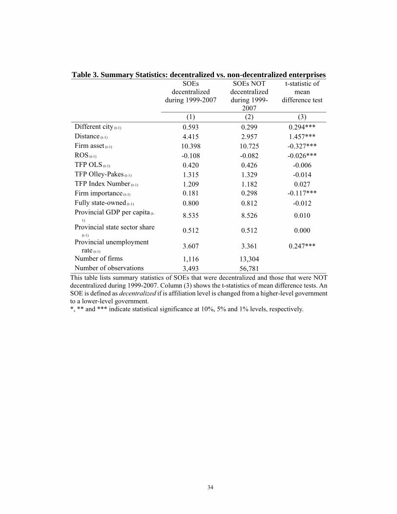
We first, in Table 3, compare how decentralized and non-decentralized SOEs differ
in basic characteristics.14 Relative to non-decentralized SOEs, the decentralized
ones are much more likely to be in different cities from the oversight governments
(59% vs. 30%), their logarithm of distance to the oversight government is much
larger (4.4 vs. 3.0), their average asset size is slightly smaller, their performance is
significantly worse in terms of labor productivity and profitability (but not TFP),
their relative importance (i.e., the share of their value added in the oversight
government’s portfolio of SOEs) is lower, and the urban unemployment rates of
their location tend to be slightly higher. The picture that emerges is that the
oversight government tends to decentralize SOEs that are far away, smaller, less
important, and worse-performing. The pattern is roughly consistent with our
predictions in the conceptual framework.
In Table 4, we compare the incidence of SOE decentralization for central,
provincial and municipal SOEs that are located in the same city as the oversight
government with those that are located at different cities. The incidence is much
higher when the firm is located in different cities from the oversight government
14 Tables 1 and 2 contain the definitions of the variables and the summary statistics.
18
than when it is in the same city: 15.6 vs. 5.5 percent for central SOEs, 15.4 vs. 5.3
percent for provincial SOEs, and 11.4 vs. 4.2 percent for municipal SOEs. This
pattern is consistent with our prediction that a larger distance to the oversight
government leads to more decentralization.
Table 5 presents the baseline probit results. The magnitudes reported are
the marginal effects on the probability of decentralization. In the first four columns,
we present the results for the whole sample, and for the central SOEs, provincial
SOEs, and municipal SOEs, respectively, to see if distance matters similarly within
each oversight category. In the last four columns, we re-do the analysis using the
dummy variable of being in a different city from the oversight government instead
of the continuous measure of distance.
Distance (in log) is robustly positively correlated with decentralization,
regardless if we use the full or oversight-specific samples. Based on column (1) for
the pooled sample, increasing distance by one standard deviation (2.24) would
increase the probability of decentralization by 1.41 percentage points (or 10% of
the standard deviation of the dependent variable). The positive distance-
decentralization link remains true when we estimate the relationship for central,
provincial, and municipal SOEs, respectively. The coefficient of distance is
especially large for municipal SOEs. For the central, provincial, and municipal
SOEs, increasing distance by one standard deviation (1.54, 1.61, and 1.49) would
increase the probability of decentralization by 0.75, 0.68, and 0.81 percentage
points, or 4%, 5% and 7% of the standard deviation.
Relying on the dummy version of distance, when an SOE is located in a
different city from the oversight government, the probability of decentralization
increases by 2.72 percentage points for the pooled sample, and 1.87, 1.47, and 4.4
percentage points for central, provincial and municipal SOEs, respectively. These
numbers translate into 20%, 10%, 10%, and 4% increase in probability of
decentralization in terms of their standard deviations for the pooled, central,
19
provincial, and municipal SOEs.
Based on the pooled sample, other determinants of decentralization
behave similarly as we observed in the decentralization vs. non-decentralization
samples comparisons. That is, decentralization is more likely for smaller firms.
Consistent with prediction 1, decentralization is more likely for worse-performing
firms and for less important firms. However, these auxiliary controls do not behave
consistently across oversight status. Thus, the effect of distance between SOEs and
their oversight government seems to be more robust than other forces such as
control benefits (i.e., firm importance) and fiscal burden (i.e., lagged firm
performance).
It is useful to know that our results are robust to whether we include the
privatized periods in our sample or not. In our baseline and the rest of paper (except
in this paragraph), we delete the periods in which an SOE became privatized—for
a firm that experienced privatization in the sample periods, the periods after the
first year of privatization are automatically dropped, since, as in the case of
decentralization, privatization was largely irreversible in our sample periods. To see
whether our key results are sensitive to the inclusion of the observations underlying
the period of privatization, we conduct a sensitivity check. Here (and only here) we
keep the “just privatized” year for an SOE. Now we have to empirically model a
three-way choice: non-decentralized (the base scenario), decentralized, and
privatized. We thus estimate the choice problem with multinomial logit model, with
non-decentralized as the base category. The set of explanatory variables are the
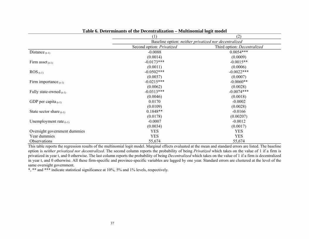
same as in the baseline scenario in Table 5. The result in Table 6 show that the
distance between the firm and its original oversight government significantly
increase the likelihood of decentralization, continuing to offer support to our
conjecture; yet the same distance is not significantly related to the likelihood of
privatization. Our key result thus remains intact whether or not we include the
sample of “privatization years”.

20
3.4. Omitted Variables, Agglomeration and Endogeneity
A potential concern is that the decentralization decisions may be affected by
particular circumstances faced by both the original oversight government and, in
the case of decentralization, the final oversight government at lower level. In such
cases, the estimated effect of distance may only reflect the impact of omitted local
economic environment. We thus, for all three subsamples of central, provincial, and
municipal SOEs, include fiscal revenue per capita, GDP per capita, and fiscal
autonomy (i.e., the ratio of fiscal revenue to fiscal expenditure in the firm’s
county)—for both the original oversight government and the government level
immediately below it.15 The results are shown in Table 7.16 These additional
oversight control variables barely matter in general, and the results on the distance
are similar to those in Table 4. Omitted variables related to fiscal circumstances of
the governments thus cannot explain the distance-decentralization link.
In China, political and economic centers tend to overlap. Beijing is not only
the political center but also a top (economic) agglomeration center. Similarly,
provincial capitals tend to be the largest cities in the provinces. Thus, a natural
concern is that the distance to oversight government really measures the distance
to major economic agglomeration. A priori there are no strong reasons why
proximity to economic centers would matter for whether an SOE should be
governed in a decentralized way. Still, this is a relevant concern that we should take
seriously.
If this concern is valid, we should expect the distance of an SOE to other
major agglomeration centers in the same oversight region to have positive effect on
15 For the central SOEs sample, we do not include these additional variables for the original oversight government because there is only one central government, and these additional variables would be perfectly collinear with the year dummies, which we have already controlled for. 16 Since we don’t have fiscal data of prefectural and county governments in 2006 and 2007, regressions in Column 2 and 3 use the sample from 1998 to 2005.
21
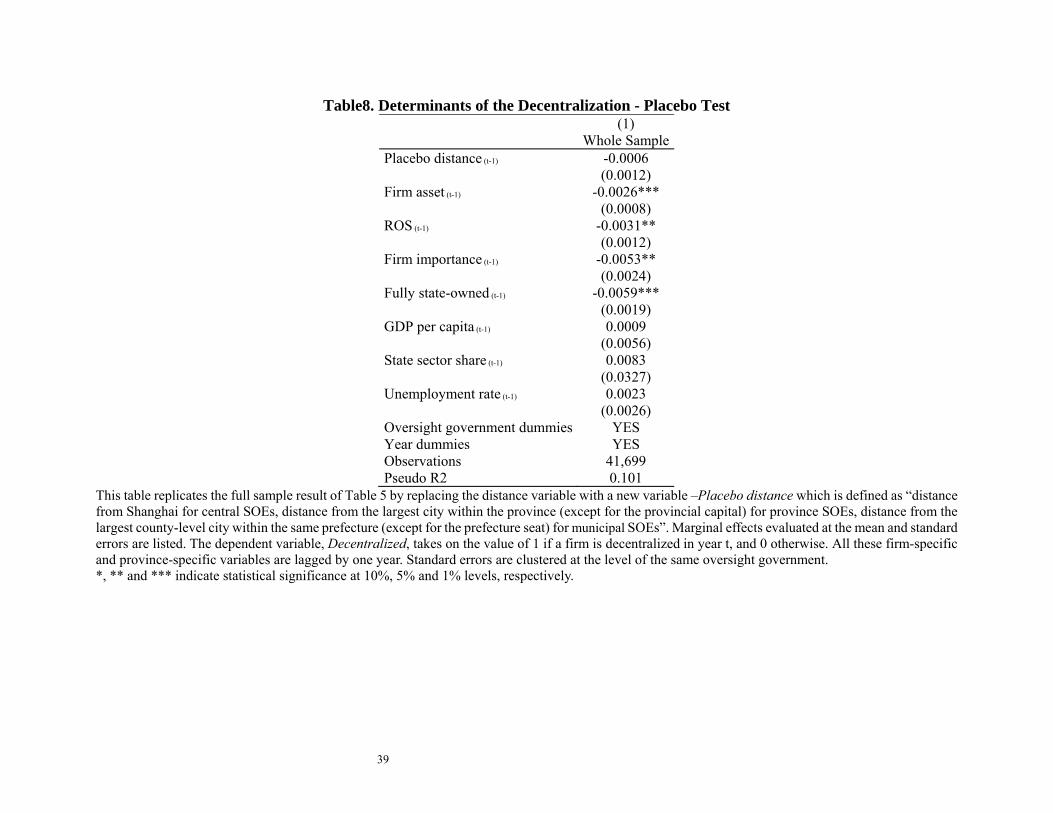
decentralization. To test the validity of this concern, we create a placebo distance
measure (Placebo Distance) as follows. For central SOEs, Placebo Distance is the
distance to Shanghai, another agglomeration center on par with the capital city of
Beijing. For provincial SOEs, Placebo Distance is the distance to the largest city
(other than the provincial capital) in the province. For municipal SOEs, Placebo
Distance is the distance to the largest county-level city (other than the city seat)
within the same prefecture. We re-run our baseline regressions using Placebo
Distance to replace the real distance, and the results are in Table 8. For the pooled
sample, Placebo Distance is completely insignificant. Thus, our key result on the
positive effect of distance on decentralization of SOEs is not due to economic
agglomeration.
Another relevant concern is that the distance of an SOE to its oversight
government may be endogenous. For instance, far-away SOEs may be
systematically less important. To examine this possibility, we now try to find
exogenous source of variations for the distance. We exploit a large wave of SOE
migration that took place in the 1960s and the 1970s due to the so-called Third
Front Construction (TFC) program. TFC was implemented in response to the
perceived threat from Soviet Union and U.S for major wars (Figure 2 shows the
number of firms established under this program during 1961-1985). This
exogenously changed the distance of many SOEs to their oversight government.
We thus construct a dummy variable Third Front, which is one if a firm was
established during 1964-1966 or 1969-1972 in the TFC Region (Li and Long, 2013).
Table 9 reports the IV regression results using various specifications. In
general, our instrument seems to be valid and generates meaningful results. In the
first stage regressions, we get significant positive effects of the TFC dummy on
distance, suggesting that the politically-motivated TFC relocation did increase the
distance between the firm and the oversight government. Distance gets the same
positive and significant effect on the likelihood of decentralization in the second-

22
stage regressions. When we only control for province dummies, the first-stage F-
statistics is 18.48 (column 1). When we put more controls and include all the 363
oversight government dummies, which likely takes away a significant portion of
the variations in Distance, the F-statistics drops to 4.85 (columns 4 and 6). However,
even in this case the IV regressions do pass the Anderson-Rubin test, suggesting
that the variable Distance is significant even in the event of weak IV (see column
6). Nevertheless, we note that the qualitative results of a significant positive effect
of Distance on decentralization remain intact. Since the results from the IV probit
and the two-stage least square (2SLS) models are similar, we shall focus on the
2SLS results. As expected, being a Third-Front-Construction SOE would increase
log distance by 0.19, and it is statistically significant at the 5% level. Once corrected
for endogeneity, the distance remains exerting a positive influence on
decentralization, and the coefficient increases to 0.03 (from 0.006). The results thus
confirm the key importance of the distance between enterprises and their oversight
government.
3.5 The Mechanisms of Distance on Decentralization
In the conceptual framework, we predict that the decentralization-distance link
would be stronger for firms with higher communication costs or with higher
performance uncertainty. To test this, we need measurements.
We proxy communication costs by three measures. The first is provincial
road mileage (road mileage per capita): more convenient transportation
significantly reduces the difficulty of on-site inspection, and thus makes
information more accurate. The second is provincial telecom density, i.e., the share
of people having either mobile or fixed phones. The third is the share of people
using internet.
We proxy high uncertainty over a firm by several variables: the average
share of intangible assets in total assets within the firm’s industry, and several

23
measures of the dispersion of firm performance within the firm’s industry. A higher
share of intangible assets for a firm in general implies higher uncertainty about the
firm’s technology and performance. Since we rely on three different ways to
compute TFP—the OLS production function method, the Olley-Pakes method, and
the index function method—we present three sets of results for the distance-TFP-
dispersion specification (see the data appendix for the details of the construction of
TFP). In addition, we also present the dispersion in return-to-sales (ROS, that is,
before-tax profit over sales), which is more transparent.
The results in Table 10 strongly support our conjecture. Indeed, lower
communication costs are associated with a reduced importance of distance in
determining decentralization. The interaction with provincial road mileage, our
proxy of communication costs, is statistically significant (see column 1).
Increasing provincial road density at the mean by one standard deviation is
associated with a reduction in by 38 percent. The results are qualitatively
similar when we use provincial telecom density, or internet density. Furthermore,
uncertainty about the firm is associated with an increase the importance of distance
in determining decentralization. The interactions of distance with our proxies of
uncertainty about the firm are all positive and statistically significant. Increasing
dispersion of industry TFP (calculated by Olley-Pakes method) at the mean by one
standard deviation would increase by almost 120 percent.17 Increasing
average intangibility ratio of the industry at the mean by one standard deviation is
associated with an increase in by 10 percent. These findings put in
perspective the relative magnitudes of the two mechanisms. It seems that both
mechanisms are qualitatively important, and uncertainty about firm performance is
perhaps somewhat more important.
17 The corresponding increase when using dispersion of TFP based on the index function method is almost 130 percent.

24
Overall, results in this section suggest that an SOE is more likely to be
decentralized if it lies far away from the oversight government. The effect of
distance is larger when there is more uncertainty about the firm and when
communication costs are higher.
4. Conclusions
China’s decentralization of SOEs represents a unique chance to test the implications
of Hayek’s insight on the importance of local information for designing an
economic system. As the opening quote of Hayek suggests, when a society is
experiencing rapid changes, the ultimate decisions should be left to those familiar
with the particular circumstances, and “some form of decentralization” is needed.
Indeed, we find that a larger information asymmetry between the original oversight
government and the SOE, as proxied by their physical distance, is associated with
a greater likelihood of decentralization. Moreover, the positive effect of distance on
decentralization is larger where SOE performance is more uncertain and
communication costs are higher. Our findings suggest that Hayek’s insight on local
information is a key for understanding the efficiency of firms in general and
economic systems in particular.
Reference
Agarwal, S. and Hauswald, R. 2010. “Distance and Private Information in Lending,”
Review of Financial Studies. 23(7): 2757-2788.
Acemoglu, D., P. Aghion, C. Lelarge, J. Van Reenen, and F. Zilibotti, 2007,
“Technology, information, and the decentralization of the firm”, Quarterly
Journal of Economics, 122(4), 1759-1799.
25
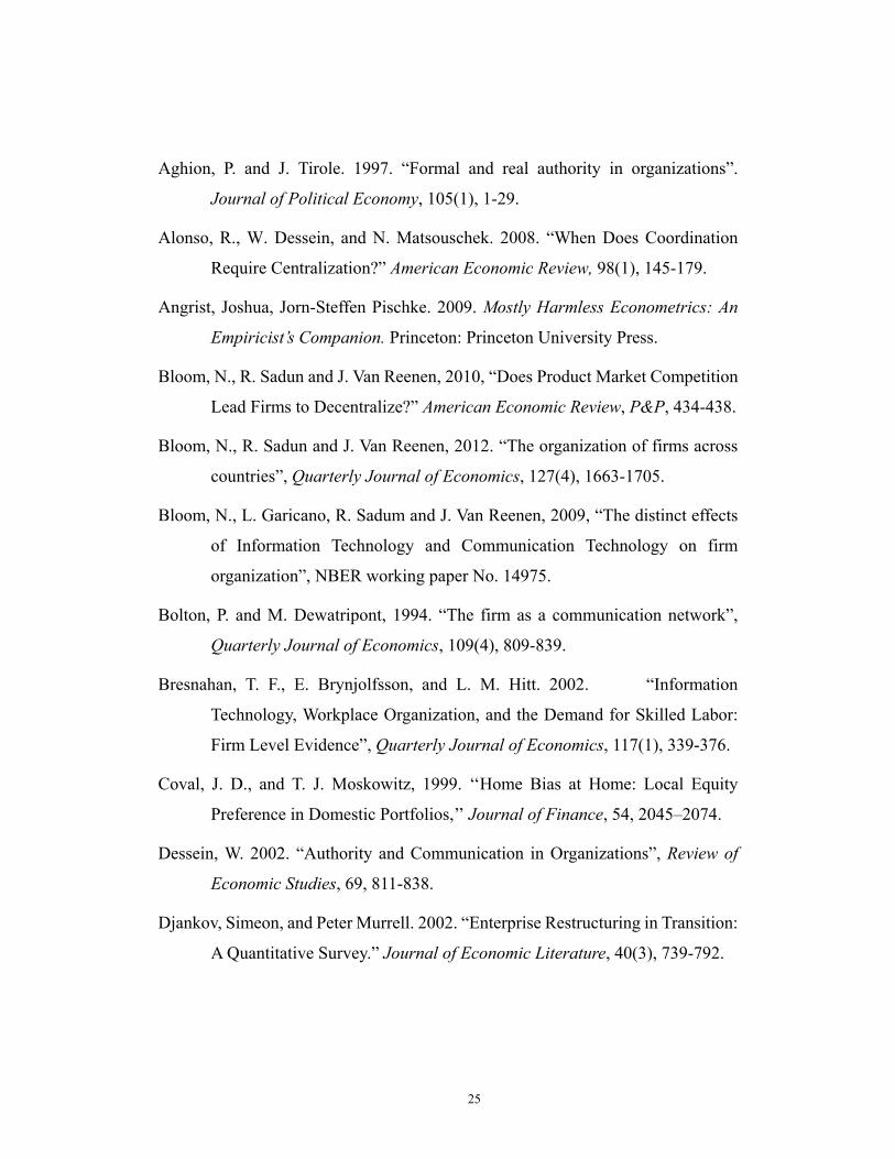
Aghion, P. and J. Tirole. 1997. “Formal and real authority in organizations”.
Journal of Political Economy, 105(1), 1-29.
Alonso, R., W. Dessein, and N. Matsouschek. 2008. “When Does Coordination
Require Centralization?” American Economic Review, 98(1), 145-179.
Angrist, Joshua, Jorn-Steffen Pischke. 2009. Mostly Harmless Econometrics: An
Empiricist’s Companion. Princeton: Princeton University Press.
Bloom, N., R. Sadun and J. Van Reenen, 2010, “Does Product Market Competition
Lead Firms to Decentralize?” American Economic Review, P&P, 434-438.
Bloom, N., R. Sadun and J. Van Reenen, 2012. “The organization of firms across
countries”, Quarterly Journal of Economics, 127(4), 1663-1705.
Bloom, N., L. Garicano, R. Sadum and J. Van Reenen, 2009, “The distinct effects
of Information Technology and Communication Technology on firm
organization”, NBER working paper No. 14975.
Bolton, P. and M. Dewatripont, 1994. “The firm as a communication network”,
Quarterly Journal of Economics, 109(4), 809-839.
Bresnahan, T. F., E. Brynjolfsson, and L. M. Hitt. 2002. “Information
Technology, Workplace Organization, and the Demand for Skilled Labor:
Firm Level Evidence”, Quarterly Journal of Economics, 117(1), 339-376.
Coval, J. D., and T. J. Moskowitz, 1999. ‘‘Home Bias at Home: Local Equity
Preference in Domestic Portfolios,’’ Journal of Finance, 54, 2045–2074.
Dessein, W. 2002. “Authority and Communication in Organizations”, Review of
Economic Studies, 69, 811-838.
Djankov, Simeon, and Peter Murrell. 2002. “Enterprise Restructuring in Transition:
A Quantitative Survey.” Journal of Economic Literature, 40(3), 739-792.

26
Estrin S, Hanousek J, Kočenda E, Svejnar, J., 2009. “The effects of privatization
and ownership in transition economies.” Journal of Economic Literature,
47(3), 699-728.
Estrin, S. and V. Perotin, 1991. “Does ownership always matter?” International
Journal of Industrial Organization, 9(1), 55–73.
Garicano, L. 2000. “Hierarchies and the Organization of Knowledge in Production”,
Journal of Political Economy, 108(5), 874-904.
Garicano, L. and E. Rossi-Hansberg. 2006. “Organization and inequality in a
knowledge economy”. Quarterly Journal of Economics, 121, 1383-1435.
Garmaise, M. and T. Moskowitz, 2004, “Confronting Information Asymmetries:
Evidence from Real Estate Markets,” Review of Financial Studies, 16(4),
1007-1040.
Giroud, X. 2013, “Proximity and investment: evidence from plant-level data”.
Quarterly Journal of Economics, 128(2), 861-915.
Grinblatt, M. and M. Keloharju 2001. “How Distance, Language, and Culture
Influence Stockholdings and Trades,” Journal of Finance, 56, 1053-1073.
Li, Lixing and Guangrong Ma 2015. “Government Size and Tax Evasion:
Evidence from China.” Pacific Economic Review, 20(2), 346-364.
Li, Yunsen and Cheryl Long 2013. “Historical Events and Regional Development:
Evidence from China’s Third Front Construction.” Manuscript, Xiamen
University.
Markevich, A. and E. Zhuravskaya, 2011, “M-form hierarchy with poorly-
diversified divisions: A case of Khrushchev’s reform in Soviet Russia”,
Journal of Public Economics 95, 1550-1560.

27
Maskin, E., Y. Qian and C. Xu. 2002. “Incentives, Information, and
Organizational Form,” Review of Economic Studies, 67, 359-378.
Mian, Atif, 2006. “Distance Constraints: The Limits of Foreign Lending in Poor
Economies”, Journal of Finance, 61, 1465–1505.
Nie, Huihua and Minjie Jiang, 2011. “Coalmine Accidents and Collusion between
Local Government and Firms: Evidence from Provincial Level Panel Data in
China,” Economic Research Journal (in Chinese), 6, 146-156.
Petersen, Mitchell A., and Raghuram Rajan, 1994, “The benefits of firm-Evidence
from small-business data”, Journal of Finance 49, 3–37.
Petersen, M. A., and R. G. Rajan, 2002. ‘‘Does Distance Still Matter? The
Information Revolution in Small Business Lending,’’ Journal of Finance, 57,
2533–2570.
Qian, Yingyi. 2000 “The process of China’s market transition (1978-1998): The
evolutionary, historical, and comparative perspectives,” Journal of
Institutional and Theoretical Economics, 156(1), 151-171.
Qian, Y., G. Roland, C. Xu. 2006. “Coordination and experimentation in M-Form
and U-Form Organizations,” Journal of Political Economy 114, 366-402.
Qian, Yingyi, Gerard Roland, Chenggang Xu, 1993. “Why China’s Economic
Reforms Differ: The M-Form Hierarchy and Entry/Expansion of the Non-
State Sector,” Economics of Transition, 1(2), 135-170.
Samuelson, Paul, 1973. Economics 9th Edition, McGraw Hill.
Shleifer, A., and R. W. Vishny, R. W., 1994. “Politicians and firms.” Quarterly
Journal of Economics 109 (4), 995–1025.
28
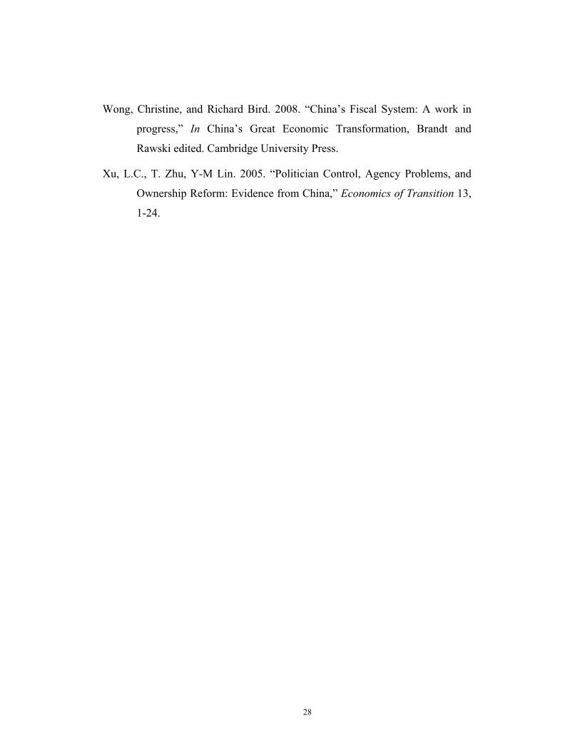
Wong, Christine, and Richard Bird. 2008. “China’s Fiscal System: A work in
progress,” In China’s Great Economic Transformation, Brandt and
Rawski edited. Cambridge University Press.
Xu, L.C., T. Zhu, Y-M Lin. 2005. “Politician Control, Agency Problems, and
Ownership Reform: Evidence from China,” Economics of Transition 13,
1-24.

29
Figure 1. Hierarchy of China’s SOEs Affiliation
Note: This figure shows the distribution of SOE affiliations in terms of number of firms, employment and output. Source: Author’s calculation from China Industrial Firm Database, 1998.

30
Figure 2. Number of New Firms in “Third Front Construction” Area during
1961-1985
Source: The data is from Annual Survey of Industrial Firms (ASIF).
31
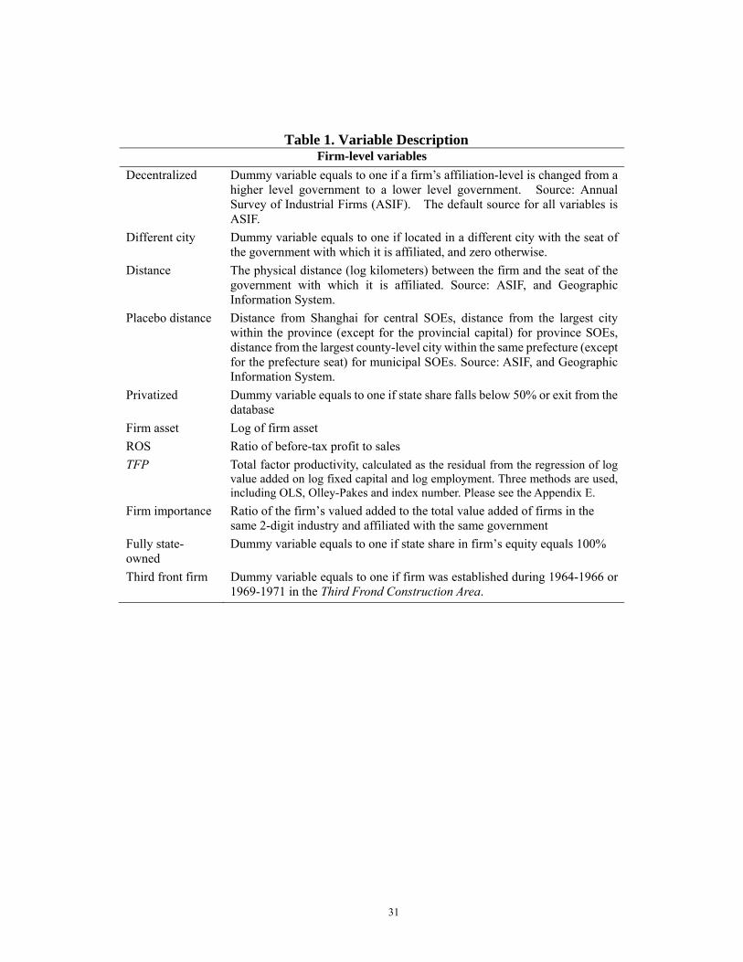
Table 1. Variable Description Firm-level variables
Decentralized Dummy variable equals to one if a firm’s affiliation-level is changed from a higher level government to a lower level government. Source: Annual Survey of Industrial Firms (ASIF). The default source for all variables is ASIF.
Different city Dummy variable equals to one if located in a different city with the seat of the government with which it is affiliated, and zero otherwise.
Distance The physical distance (log kilometers) between the firm and the seat of the government with which it is affiliated. Source: ASIF, and Geographic Information System.
Placebo distance Distance from Shanghai for central SOEs, distance from the largest city within the province (except for the provincial capital) for province SOEs, distance from the largest county-level city within the same prefecture (except for the prefecture seat) for municipal SOEs. Source: ASIF, and Geographic Information System.
Privatized Dummy variable equals to one if state share falls below 50% or exit from the database
Firm asset Log of firm asset
ROS Ratio of before-tax profit to sales
TFP Total factor productivity, calculated as the residual from the regression of log value added on log fixed capital and log employment. Three methods are used, including OLS, Olley-Pakes and index number. Please see the Appendix E.
Firm importance Ratio of the firm’s valued added to the total value added of firms in the same 2-digit industry and affiliated with the same government
Fully state-owned
Dummy variable equals to one if state share in firm’s equity equals 100%
Third front firm Dummy variable equals to one if firm was established during 1964-1966 or 1969-1971 in the Third Frond Construction Area.

32
Table 1. (Cont’d)
Fiscal and Economic Variables in Province, Prefecture and City levels
Province GDP per capita
Annual per capita GDP in the firm’s province, constant price in the year 2000. Source: China Statistical yearbooks.
Province state sector share
Percentage of employment in SOEs in total urban employment in the firm’s province. Source: China Statistical yearbooks.
Province unemployment rate
Annual urban employment rate in the firm’s province. Source: China Statistical yearbooks.
Province fiscal revenue p.c.
Annual per capita fiscal revenue in the firm’s province. Source: China Statistical Yearbooks.
Province fiscal autonomy
Ratio of fiscal revenue to fiscal expenditure in the firm’s province. Source: China Statistical Yearbooks.
Prefecture GDP per capita
Annual per capita GDP in the firm’s prefecture. Source: Public Finance Statistical Materials of Prefectures, Cities, and Counties (1998-2005).
Prefecture fiscal revenue per capita
Annual per capita GDP fiscal revenue in the firm’s prefecture. Source: Public Finance Statistical Materials of Prefectures, Cities, and Counties (1998-2005).
Prefecture fiscal autonomy
Ratio of fiscal revenue to fiscal expenditure in the firm’s prefecture. Source: Public Finance Statistical Materials of Prefectures, Cities, and Counties (1998-2005).
County GDP p.c. Annual per capita GDP in the firm’s county. Source: Public Finance Statistical Materials of Prefectures, Cities, and Counties (1998-2005).
County fiscal revenue per capita
Annual per capita GDP fiscal revenue in the firm’s county. Source: Public Finance Statistical Materials of Prefectures, Cities, and Counties (1998-2005).
County fiscal autonomy
Ratio of fiscal revenue to fiscal expenditure in the firm’s county. Source: Public Finance Statistical Materials of Prefectures, Cities, and Counties (1998-2005).
TFP dispersion Standard deviation of firm TFP in the same 3-digit industry
ROS dispersion Standard deviation of firm ROS in the same 3-digit industry
Intangibility Average ratio of intangible assets to firm total assets in the same 3-digit industry
Province telecom infrastructure
Per capita number of mobile phone and fixed telephone users
Province internet infrastructure
Per capita number of internet users
Province road mileage
Per capita road mileage. Different levels of roads and railway are translated into the equivalent of second-level road according to transport capacity.

33
Table 2. Summary Statistics
Obs Mean S.D. Min Max
Firm-level Variables
Decentralized 60274 0.019 0.135 0.000 1.000
Different city 58076 0.304 0.460 0.000 1.000
Distance 58076 2.984 2.238 0.000 8.129
Firm asset 60274 10.719 1.897 0.662 19.892
Firm age 60143 3.151 0.839 0.000 7.602
ROS 59150 -0.171 0.501 -5.259 0.416
Labor Productivity 56993 2.946 1.261 -7.496 6.368
TFP OLS 56144 0.426 1.354 -10.698 12.276
TFP Olley-Pakes 48778 1.328 1.474 -9.930 9.483
TFP Index Number 56144 1.182 1.411 -9.766 12.085
Firm importance 59988 0.310 0.381 0.000 1.000
Fully state-owned 60274 0.818 0.385 0.000 1.000
Third front firm 60274 0.056 0.230 0.000 1.000
Province-level Variables
GDP per capita 60264 8.531 0.532 7.234 10.160
State sector employment share 60264 0.511 0.109 0.173 0.794
Unemployment rate 60264 3.386 0.878 0.620 6.800
Road mileage 60264 13.711 8.017 3.936 63.554
Telecom infrastructure 60264 7.712 0.813 5.597 9.659
Internet users 60264 4.490 2.139 -1.446 7.993
Industry-level Variables
Intangibility 60274 0.015 0.009 0.000 0.068
ROS dispersion 60274 0.132 0.036 0.057 0.269
TFP OLS dispersion 60274 1.215 0.184 0.736 2.193 TFP Olley-Pakes dispersion 52496 1.165 0.165 0.749 2.094
TFP Index Number dispersion 60274 1.147 0.174 0.660 2.068
34
Table 3. Summary Statistics: decentralized vs. non-decentralized enterprises SOEs
decentralized during 1999-2007
SOEs NOT decentralized during 1999-
2007
t-statistic of mean
difference test
(1) (2) (3) Different city (t-1) 0.593 0.299 0.294*** Distance (t-1) 4.415 2.957 1.457*** Firm asset (t-1) 10.398 10.725 -0.327*** ROS (t-1) -0.108 -0.082 -0.026*** TFP OLS (t-1) 0.420 0.426 -0.006 TFP Olley-Pakes (t-1) 1.315 1.329 -0.014 TFP Index Number (t-1) 1.209 1.182 0.027 Firm importance (t-1) 0.181 0.298 -0.117*** Fully state-owned (t-1) 0.800 0.812 -0.012 Provincial GDP per capita (t-
1) 8.535 8.526 0.010
Provincial state sector share
(t-1) 0.512 0.512 0.000
Provincial unemployment rate (t-1)
3.607 3.361 0.247***
Number of firms 1,116 13,304 Number of observations 3,493 56,781
This table lists summary statistics of SOEs that were decentralized and those that were NOT decentralized during 1999-2007. Column (3) shows the t-statistics of mean difference tests. An SOE is defined as decentralized if is affiliation level is changed from a higher-level government to a lower-level government. *, ** and *** indicate statistical significance at 10%, 5% and 1% levels, respectively.

35
Table 4. Decentralization Ratio by Location and Affiliation
Ratio of Decentralization
SOEs located in the SAME city with the seat
of the government
SOEs located in a DIFFERENT city with the
seat of the government
Central SOEs 5.53% 15.63% (253) (1945)
Province SOEs 5.33% 15.35% (2231) (1726)
Municipal SOEs 4.17% 11.38% (7298) (967)
This table compares ratio of decentralization of SOEs located in the same city with the seat of the government with which it is affiliated and SOEs that are located in a different city. Number of firms in each subsample is listed in brackets. A firm is decentralized if its affiliation level is lowered.

36
Table 5. Determination of Decentralization - Baseline Results (1)
Whole Sample (2)
Central SOE (3)
Province SOE (4)
Municipal SOE (5)
Whole Sample (6)
Central SOE (7)
Province SOE (8)
Municipal SOE Distance (t-1) 0.0063*** 0.0049** 0.0042*** 0.0055***
(0.0008) (0.0022) (0.0007) (0.0009)
Different City (t-1) 0.0272*** 0.0187*** 0.0147*** 0.0444***
(0.0030) (0.0047) (0.0030) (0.0092)
Firm asset (t-1) -0.0024*** -0.0036*** -0.0020*** -0.0020*** -0.0025*** -0.0037*** -0.0021*** -0.0018***
(0.0007) (0.0010) (0.0005) (0.0006) (0.0007) (0.0009) (0.0005) (0.0007)
ROS (t-1) -0.0030*** -0.0020 -0.0032*** -0.0016 -0.0033*** -0.0023 -0.0034*** -0.0022**
(0.0012) (0.0037) (0.0010) (0.0010) (0.0012) (0.0037) (0.0010) (0.0011)
Firm importance (t-1) -0.0040* 0.0333 -0.0046 -0.0039* -0.0045* 0.0330 -0.0048 -0.0044*
(0.0023) (0.0321) (0.0032) (0.0024) (0.0023) (0.0325) (0.0033) (0.0024)
Fully state-owned (t-1) -0.0055*** -0.0001 -0.0138*** -0.0015 -0.0061*** -0.0003 -0.0142*** -0.0017
(0.0018) (0.0052) (0.0035) (0.0017) (0.0018) (0.0054) (0.0035) (0.0017)
GDP per capita (t-1) 0.0084 -0.0050 -0.0661** 0.0931** 0.0058 -0.0057 -0.0679** 0.0977**
(0.0056) (0.0064) (0.0300) (0.0383) (0.0050) (0.0059) (0.0295) (0.0416)
State sector share (t-1) 0.0181 -0.0794** 0.1210*** 0.0612 0.0155 -0.0811*** 0.1256*** 0.0631
(0.0344) (0.0326) (0.0360) (0.0397) (0.0300) (0.0281) (0.0363) (0.0406)
Unemployment rate (t-1) -0.0004 0.0030 0.0001 -0.0017 -0.0002 0.0020 -0.0000 -0.0022
(0.0017) (0.0028) (0.0034) (0.0019) (0.0020) (0.0037) (0.0033) (0.0020)
Year dummies YES YES YES YES YES YES YES YES
Oversight government
dummies
YES YES YES YES YES YES YES YES
Observations 41,681 8,724 15,681 16,727 41,681 8,724 15,681 16,727
Pseudo R-squared 0.120 0.0858 0.157 0.188 0.118 0.0854 0.156 0.186 This table reports probit regression results on the determination of SOE decentralization. Marginal effects on the probability of decentralization that are evaluated at the mean and their standard errors are listed. All these firm-specific and province-specific variables are lagged by one year. Standard errors are clustered at the level of the same oversight government. *, ** and *** indicate statistical significance at 10%, 5% and 1% levels, respectively.
37
Table 6. Determinants of the Decentralization – Multinomial logit model (1) (2)
Baseline option: neither privatized nor decentralized Second option: Privatized Third option: Decentralized
Distance (t-1) -0.0088 0.0054*** (0.0014) (0.0009)
Firm asset (t-1) -0.0173*** -0.0015** (0.0011) (0.0006)
ROS (t-1) -0.0502*** -0.0022*** (0.0037) (0.0007)
Firm importance (t-1) -0.0215*** -0.0060** (0.0062) (0.0028)
Fully state-owned (t-1) -0.0313*** -0.0074*** (0.0046) (0.0018)
GDP per capita (t-1) 0.0170 -0.0002 (0.0109) (0.0028)
State sector share (t-1) 0.1848** -0.0166 (0.0178) (0.00207)
Unemployment rate (t-1) -0.0007 -0.0012 (0.0034) (0.0017)
Oversight government dummies YES YES Year dummies YES YES Observations 55,674 55,674
This table reports the regression results of the multinomial logit model. Marginal effects evaluated at the mean and standard errors are listed. The baseline option is neither privatized nor decentralized. The second column reports the probability of being Privatized which takes on the value of 1 if a firm is privatized in year t, and 0 otherwise. The last column reports the probability of being Decentralized which takes on the value of 1 if a firm is decentralized in year t, and 0 otherwise. All these firm-specific and province-specific variables are lagged by one year. Standard errors are clustered at the level of the same oversight government. *, ** and *** indicate statistical significance at 10%, 5% and 1% levels, respectively.

38
Table 7. Determinants of Decentralization - Additional Controls (1)
Central SOE (2)
Province SOE MDistance (t-1) 0.0047*** 0.0028*
(0.0018) (0.0015) Firm asset (t-1) -0.0037*** -0.0021**
(0.0009) (0.0011) ROS (t-1) -0.0022 -0.0031**
(0.0037) (0.0013) Firm importance (t-1) 0.0332 -0.0035
(0.0336) (0.0042) Fully state-owned (t-1) -0.0004 -0.0159***
(0.0051) (0.0050) State sector share (t-1) -0.0674** 0.2213***
(0.0305) (0.0754) Unemployment rate (t-1) 0.0024 0.0031
(0.0022) (0.0043) Original oversight government fiscal revenue per
capita (t-1) 0.0289 (0.0401)
Original oversight government GDP per capita (t-1) -0.0997* (0.0546)
Original oversight government fiscal autonomy (t-1) 0.0484 (0.0782)
Lower-level government fiscal revenue per capita
(t-1) -0.0091 -0.0002 (0.0060) (0.0064)
Lower-level government GDP per capita. (t-1) 0.0053 -0.0019 (0.0103) (0.0061)
Lower-level government fiscal autonomy (t-1) 0.0102 -0.0210 (0.0267) (0.0185)
Observations 8,724 10,328 Oversight government dummies YES YES Year dummies YES YES Pseudo R-squared 0.0867 0.153
This table additionally controls for per capita GDP, fiscal revenue, and fiscal autonomy of the government with which the firm iTable 1 for definitions). Column 1-3 are the results for the regression on the subsample of central SOEs, province SOEs and munWe report marginal probabilities evaluated at the mean of the variables. Standard errors are clustered at the level of the same ove*, ** and *** indicate statistical significance at 10%, 5% and 1% levels, respectively.
39
Table8. Determinants of the Decentralization - Placebo Test (1)
Whole Sample Placebo distance (t-1) -0.0006
(0.0012) Firm asset (t-1) -0.0026***
(0.0008) ROS (t-1) -0.0031**
(0.0012) Firm importance (t-1) -0.0053**
(0.0024) Fully state-owned (t-1) -0.0059***
(0.0019) GDP per capita (t-1) 0.0009
(0.0056) State sector share (t-1) 0.0083
(0.0327) Unemployment rate (t-1) 0.0023
(0.0026) Oversight government dummies YES Year dummies YES Observations 41,699 Pseudo R2 0.101
This table replicates the full sample result of Table 5 by replacing the distance variable with a new variable –Placebo distance which is defined as “distance from Shanghai for central SOEs, distance from the largest city within the province (except for the provincial capital) for province SOEs, distance from the largest county-level city within the same prefecture (except for the prefecture seat) for municipal SOEs”. Marginal effects evaluated at the mean and standard errors are listed. The dependent variable, Decentralized, takes on the value of 1 if a firm is decentralized in year t, and 0 otherwise. All these firm-specific and province-specific variables are lagged by one year. Standard errors are clustered at the level of the same oversight government. *, ** and *** indicate statistical significance at 10%, 5% and 1% levels, respectively.

40
Table 9. Determinants of Decentralization - Third Front Construction as IV IV Probit model IV Probit model 2SLS model
(1) 2nd stage (2) 1st stage (3) 2nd stage (4) 1st stage (5) 2nd stage (6) 1st stage Decentralized Distance Decentralized Distance Decentralized Distance
Distance (t-1) 0.0143** 0.0431** 0.0318* (0.0059) (0.0189) (0.0175)
Firm asset (t-1) -0.0045** 0.1864*** -0.0044*** 0.0028 -0.0031*** 0.0028 (0.0017) (0.0216) (0.0016) (0.0135) (0.0010) (0.0135)
ROS (t-1) -0.0060** 0.3160*** -0.0059** 0.0504*** -0.0050** 0.0504*** (0.0024) (0.0377) (0.0024) (0.0144) (0.0021) (0.0144)
Firm importance (t-1) 0.0204* -2.6195*** -0.0013 -0.1162*** 0.0019 -0.1162*** (0.0122) (0.1458) (0.0047) (0.0404) (0.0030) (0.0404)
Fully state-owned (t-1) -0.0079*** 0.2003*** -0.0087* -0.0057 -0.0050*** -0.0057 (0.0030) (0.0719) (0.0045) (0.0238) (0.0018) (0.0238)
GDP per capita (t-1) 0.0090 0.5752 0.0553** -1.2842** 0.0432 -1.2842** (0.0400) (0.5234) (0.0276) (0.5223) (0.0289) (0.5223)
State sector share (t-1) 0.0848 -0.7283 0.0850 -1.6849 0.0579 -1.6849 (0.05748) (0.9390) (0.0696) (1.4856) (0.0645) (1.4856)
Unemployment rate(t-1) -0.0023 0.0310 -0.0166* 0.4420* -0.0094 0.4420* (0.0036) (0.0734) (0.0094) (0.2284) (0.0100) (0.2284)
Third front firm 0.4684*** 0.1913** 0.1913** (0.1089) (0.0869) (0.0869)
Oversight government dummies YES YES YES YES Year dummies YES YES YES YES YES YES Province dummies YES YES Observations 56,700 56,700 41,684 41,684 56,705 56,705 First-stage F statistic 18.48 4.85 4.85 Anderson-Rubin test P-value
0.0937
In this table, we present the results of distance on decentralization using Third Front Construction (TFC) Dummy as the instrument. TFC equals to one if firm was established during 1964-1966 or 1969-1971 in the “Third Frond Construction Area.” Marginal effects evaluated at the mean and standard errors are listed. The dependent variable Decentralized in the 2nd stage takes on the value of 1 if a firm is decentralized in year t, and 0 otherwise. Columns 1-4 present the 2nd and 1st stage results from IV Probit model, which is estimated using conditional MLE (i.e., the first stage result is estimated jointly with the parameters of the Probit equation when implementing conditional MLE). Columns 1-2 control for province dummies. Columns 3-4 control for a full set of oversight government dummies. Columns 5-6 present results from a standard 2SLS model. Standard errors are clustered at the level of the same oversight government. *, ** and *** indicate statistical significance at 10%, 5% and 1% levels, respectively.

41
Table 10. Determinants of Decentralization – Role of Information (1) (2) (3) (4) (5) (6) (7) (8) Province road
mileages Province telecom
infrastructure Province
internet users Intangibility ROS
dispersion
TFP OLS dispersion
TFP Olley-Pakes dispersion
TFP Index Number
dispersion Distance (t-1) 0.0104*** 0.0193*** 0.0088*** 0.0052*** 0.0039*** (0.0009) -0.0006 -0.0004
(0.0010) (0.0036) (0.0013) (0.0009) (0.0011) -0.0005 (0.0026) (0.0023) Distance (t-1) *
Information Intensity
-0.0003*** -0.0017*** -0.0005*** 0.0730** 0.0192** 0.0055*** 0.0062*** 0.0058*** (0.0000) (0.0004) (0.0002) (0.0327) (0.0079) (0.0016) (0.0020) (0.0017)
Information Intensity 0.0014*** -0.0010 0.0022 -0.3068** -0.1140** -0.0286** -0.0312** -0.0289** (0.0004) (0.0072) (0.0030) (0.1488) (0.0479) (0.0117) (0.0140) (0.0122)
Other control variables YES YES YES YES YES YES YES YES Oversight government
dummies YES YES YES YES YES YES YES YES
Year dummies YES YES YES YES YES YES YES YES Observations 41,684 41,684 41,684 41,681 41,684 41,684 35,660 41,684 Pseudo R2 0.123 0.123 0.123 0.121 0.121 0.121 0.119 0.122
This table reports probit regression results on the determinants of firms’ decentralization. Marginal effects evaluated at the mean and standard errors are listed. The dependent variable takes on the value of 1 if a firm is decentralized in year t, and 0 otherwise. Standard errors are clustered at the level of the same oversight government. *, ** and *** indicate statistical significance at 10%, 5% and 1% levels, respectively.
42
On-Line Appendix: Not for Publication
Appendix A. China’s third-front industries China experienced massive relocation of industries from coastal provinces to her inland
provinces during 1960s and 1970s, known as Third Front Construction. The move was a response
to perceived military threat from USSR and USA. In August 1964, North Vietnam and U.S. navy
had a series of confrontations in the waters of Tonkin Gulf. The U.S. Congress passed the Gulf of
Tonkin Resolution, which gave President Lyndon B. Johnson the authorization to deploy forces
and commence warfare against North Vietnam. Feeling that the war might escalate and China
might eventually confront the U.S. military forces, Mao Zedong, China’s top leader then, decided
to move China’s heavy industry and other strategically important resources to China’s inland
provinces, so that they would survive in a likely air assault. The move was temporarily stopped in
1966 due to the outbreak of Cultural Revolution, and was resumed after March 1969, when China
was engaged in military conflict with USSR over Zhenbao (also known as Damansky) Island. With
Richard Nixon’s visit to China in 1972, China managed to improve her relations with the west.
This led to relief of security pressure and the Third Front Construction came to a halt afterwards.
During these two periods, 1964-1966 and 1969-1972, China relocated more than 1100 factories
and about 4 million workers to mountainous areas in West China. The result was sudden increase
in the number of SOEs in these areas during the two periods (see Figure 2).

43
Appendix B. Estimation of TFP Here we describe in detail the approaches to estimate firm-level TFP.
We use a standard log-linear Cobb-Douglas production function to estimate firm-level TFP.
Specifically, TFP of firm i in year t is the estimated residual from the regression:
(A1)
where is the logarithm of value-added, and and are the logarithms of capital and
labor, respectively. To allow for different factor intensities across industries, we estimate
equation (A1) separately for each two-digit industry.18 Accordingly, TFP can be interpreted as
the relative productivity of a plant within its industry.
Real value added is constructed by subtracting deflated input from real output. We use the
two-digit ex-factory price index from China Urban Living and Price Statistics to deflate output.
The input deflator is calculated based on available output deflators at 2-digit industry level and
information from the National Input-Output (IO) tables in 1997, 2002, and 2007. From the IO table,
we know how much inputs are needed to produce one unit of output. Then the average input price
index will be the weighted average of the price index of those inputs. Thus, to obtain the input
deflator for each industry, we calculate a weighted average of the input deflators, using as weights
the coefficients in the IO table.19
In the ASIF dataset, firms report total annual employment, but they do not report the real
capital stock. Instead, firms report the value of their fixed capital stock at original purchase
prices. As these book values are the sum of nominal values for different years, they are not equal
to the real capital stock and are not comparable across time and across firms.
Ideally, we need information on all past investments of a firm to construct the real capital
stock. This, however, we do not have. Roughly following Brandt et al. (2011), we make several
assumptions and convert the value of their capital stock at original purchase prices into real values
by the following procedures.
First, we estimate the nominal value of capital stock for each year between firm’s established
year and the first year in which the firm appears in our data set. For simplicity of presentation here,
we assume that it is 1998, the first year of our panel. We assume that the growth rate of nominal
capital stock of each firm equals to the growth rate of nominal capital stock in the corresponding
18 China’s Industrial Classification (CIC) system has 30 two-digit manufacturing industries. 19 The 1997 IO table is used to construct the input deflators of 1998-2000, and the 2002 IO table is used to construct the input deflators of 2001-2005, and the 2007 IO table is used to construct the input deflators in 2006-2007.

44
two-digit industry, which is reported by China Statistics Yearbook.20 Then, we can calculate the
nominal capital stock in 1998 from the following equation:
∏ 1 (A2)
Where is the nominal captial stock in 1998 reported in the ASIF data, s indicate the
firm’s estalished year, while is the nominal captial stock in the firm’s. And is the growth
rate of nominal capital stock in the two-digit industry in year t, which is reported by China
Statistics Yearbook. From equation (A2), we can calculate the nominal stock in each year between
firm’s established year and 1998.
Second, annual nominal investment is the change in nominal capital stock between
years, that is, .
Third, we derive the real capital stock for each year between firm’s established year and 1998.
We deflate annual nominal investment in each year into real values with the investment
deflator. China Statistics Yearbook reports the investment deflator from 1990. For years 1986-1989,
we use the investment deflator constructed by Perkins and Rawski (2008).
Fourth, we obtain the real capital stock in 1998 from the perpetual inventory method.
Specifically,
1
Where is the real capital stock in year t, and is the depreciation rate, which is estimated
by / , where s is the year of establishment for the firm.
Finally, we obtain annual real investment and real capital stock after 1998. For years after
1998, we use the observed change in the firm's nominal capital stock at original purchase prices as
our estimate of nominal annual investment, that is, the nominal annual investment is still
obtained from . Real fixed investment is obtained by deflating with the
investment deflator reported by China Statistics Yearbook. The Real capital stock is constructed
using the perpetual inventory method, that is,
is annual depreciation directly reported in ASIF database and is deflated by
investment deflator reported by China Statistics Yearbook.
In our baseline analysis, we estimate equation (A1) by ordinary least squares (OLS). We call
20 Since China Statistics Yearbook report the growth rate of nominal capital stock in the two‐digit industry from 1986, we assume firms established before 1986 are established in 1986.

45
this TFP-OLS. While this approach is common in the literature, past research has argued that OLS
estimates suffer from two endogeneity issues: simultaneity of input choice and selection biases.
These two issues will generate biased estimates of and , and therefore biased estimation of
residual in equation (A1). A variety of techniques have been suggested to address the simultaneity
and selection problems. We use the method proposed by Olley and Pakes (1996). We call this TFP-
OP.
As a robustness check, we also use a straightforward index number approach, which does not
require the estimation of any parameters. In particular, the industry-specific average wage share in
output is used to measure , and one minus this share is used to measure . The intuition is that
a cost-minimizing firm will make sure the relative factor price ratio equals the local elasticity of
substitution between inputs of the production technology. Since we do not have good comparable
data to compute factor shares based on our survey data, we rely on the estimates of factor shares
in two-digit industry level from Bentolila and Saint-Paul (2003). Bloom, Sadun and Van Reenen
(2012) use a similar treatment. We call this TFP-IN.
Overall, these three approaches yield similar qualitative results. The correlations of these
productivity measures are quite high: that between TFP-OLS and TFP-IN is 0.92; between TFP-
OLS and TFP-OP, 0.96. Thus, it is not surprising that our results in general do not hinge on how
we measure productivity.