hawkes learning systems math courseware specialists copyright © 2010 by hawkes learning...
TRANSCRIPT

HAWKES LEARNING SYSTEMS
math courseware specialists
Copyright © 2010 by Hawkes Learning
Systems/Quant Systems, Inc.
All rights reserved.
Chapter 7
Probability Distributions: Information about the Future

HAWKES LEARNING SYSTEMS
math courseware specialists
Probability Distributions: Information about the Future
Section 7.1 Types of Random Variables
Objectives:
• To define discrete random variables.
• To define continuous random variables.
• To describe probability notation.

HAWKES LEARNING SYSTEMS
math courseware specialists
• Random variable – a numerical outcome of a random process.
• Probability distribution – a model which describes a specific kind of random process.
• Discrete random variable – a random variable which has a countable number of possible outcomes.
• Continuous random variable – a random variable that can assume any value on a continuous segment(s) of the real number line.
Definitions:
Probability Distributions: Information about the Future
Section 7.1 Types of Random Variables

HAWKES LEARNING SYSTEMS
math courseware specialists
Discrete Random Variables:
• To describe a discrete random variable:
• State the variable.• List all the possible values of the variable.• Determine the probabilities of these values.
Notation for Random Variables:
• Capital letters, such as X, will be used to refer to the random variable, while small letters, such as x, will refer to specific values of the random variable. Often the specific values will be subscripted,
1 2, , ... , .nx x x
Probability Distributions: Information about the Future
Section 7.1 Types of Random Variables

HAWKES LEARNING SYSTEMS
math courseware specialists
Example:
Toss a die and observe the outcome of the toss.
First list the three steps:
• State the variable: X = the outcome of the toss of the die.
• List the possible values: 1, 2, 3, 4, 5, 6. In this case
• Determine the probability of each value.
1 1,x
Value of X Probability161616161616
1
2
3
4
5
62 2,x 3 3,x 4 4,x 5 5,x 6and 6.x
Probability Distributions: Information about the Future
Section 7.1 Types of Random Variables
HAWKES LEARNING SYSTEMS
math courseware specialists
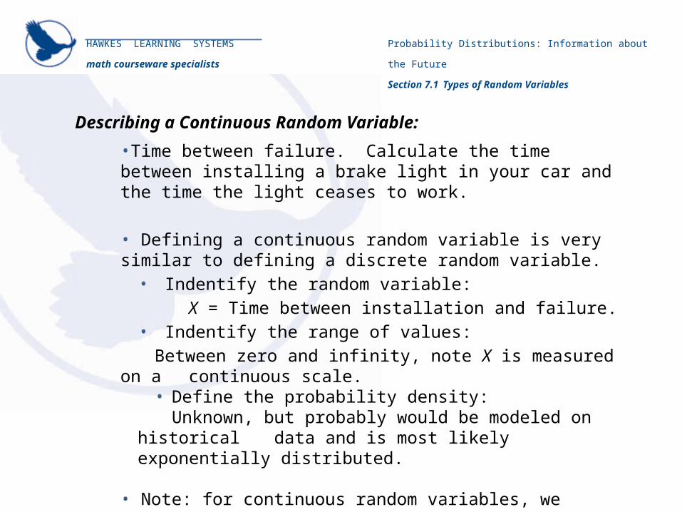
Describing a Continuous Random Variable:
•Time between failure. Calculate the time between installing a brake light in your car and the time the light ceases to work.
• Defining a continuous random variable is very similar to defining a discrete random variable.
• Indentify the random variable:
X = Time between installation and failure.• Indentify the range of values:
Between zero and infinity, note X is measured on a continuous scale.
• Define the probability density: Unknown, but probably would be modeled on historical data and is most likely exponentially distributed.
• Note: for continuous random variables, we specify probabilities with probability density functions.
Probability Distributions: Information about the Future
Section 7.1 Types of Random Variables

HAWKES LEARNING SYSTEMS
math courseware specialists
Chapter Name
Section ## Section Name
Probability Distributions: Information about the Future
Section 7.2 Discrete Probability Distributions
Objectives:
• To describe the characteristics of a discrete random variable.
HAWKES LEARNING SYSTEMS
math courseware specialists
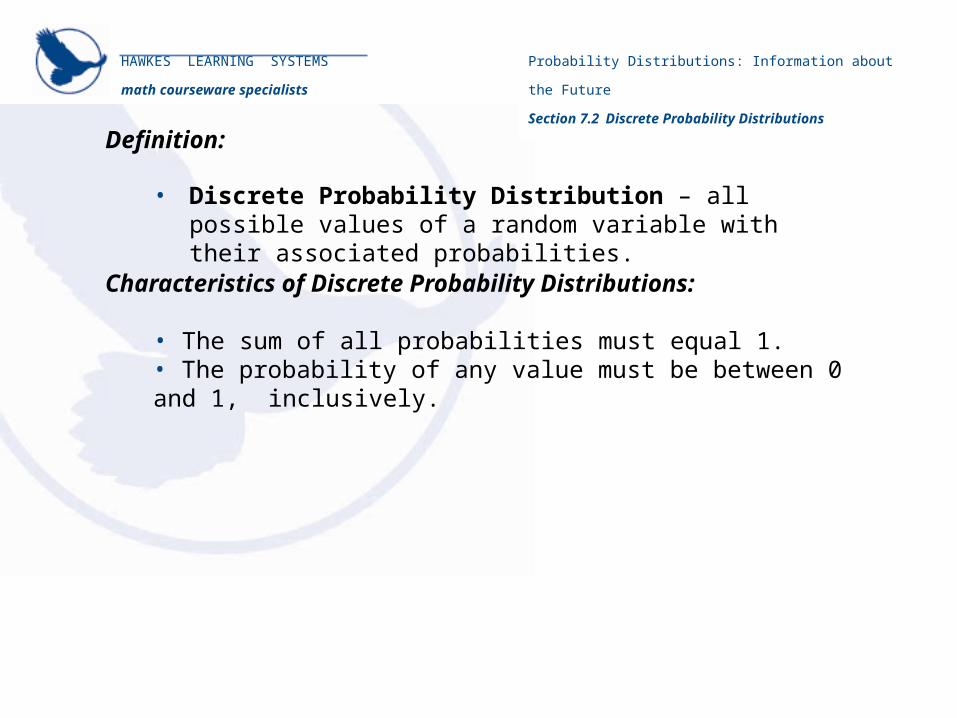
• Discrete Probability Distribution – all possible values of a random variable with their associated probabilities.
Definition:
Characteristics of Discrete Probability Distributions:
• The sum of all probabilities must equal 1.• The probability of any value must be between 0 and 1, inclusively.
Probability Distributions: Information about the Future
Section 7.2 Discrete Probability Distributions
HAWKES LEARNING SYSTEMS
math courseware specialists
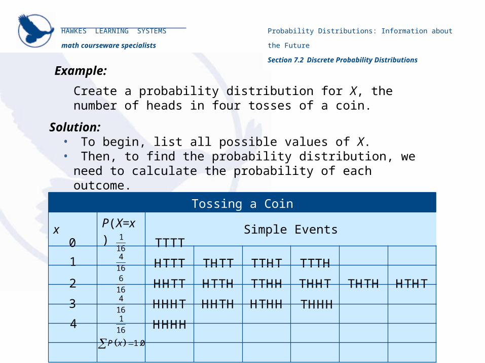
Create a probability distribution for X, the number of heads in four tosses of a coin.
Solution:• To begin, list all possible values of X.• Then, to find the probability distribution, we need to calculate the
probability of each outcome.
Tossing a Coin
x P(X=x) Simple Events
0
1
2
3
4
1
164
166
16
1
16
4
16
TTTT
HTTT
HHHH
TTHT
HHHT HHTH HTHH
TTHH THHT THTH HTHT
THTT
HTTHHHTT
THHH
TTTH
1.0P x
Probability Distributions: Information about the Future
Section 7.2 Discrete Probability Distributions
Example:

HAWKES LEARNING SYSTEMS
math courseware specialists
The probability distribution for the price of a stock thirty days from now is given below. Find the probability the price of the stock with be greater than $56.
Stock Prices
x P(X=x)
54.5 .05
55.0 .10
55.5 .25
56.0 .30
56.5 .20
57.0 .10
1.0P x
Based on the probability distribution, the probability that the stock price will be more than $56 in thirty days is calculated as follows:
56 56.5 57.0P X P X P X
.20 .10
.30
Probability Distributions: Information about the Future
Section 7.2 Discrete Probability Distributions
Example:
Solution:

HAWKES LEARNING SYSTEMS
math courseware specialists
Probability Distributions: Information about the Future
Section 7.3 Expected Value
Objectives:
• To define and describe the expected value of a discrete random variable.
HAWKES LEARNING SYSTEMS
math courseware specialists
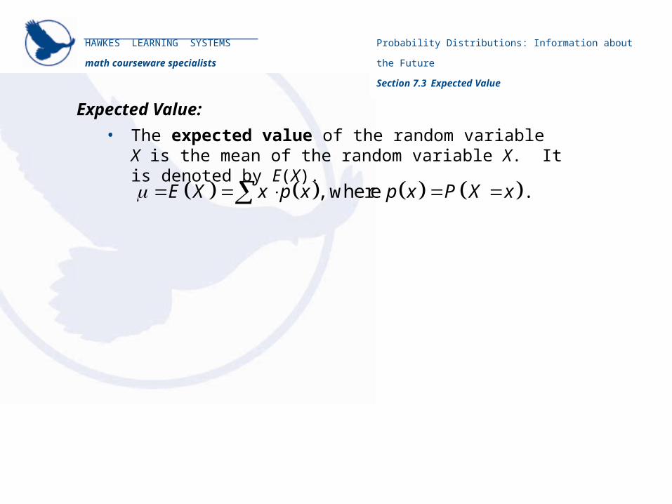
Expected Value:
• The expected value of the random variable X is the mean of the random variable X. It is denoted by E(X).
, where .E X x p x p x P X x
Probability Distributions: Information about the Future
Section 7.3 Expected Value

HAWKES LEARNING SYSTEMS
math courseware specialists
John sells cars. Calculate the expected value of the number of cars John sells per day.
Car Sales
x P(X=x)
0
1
2
3
4
.15
.30
.35
.15
.05
x X xP
Solution:
E X x P X x
0 .15 1 .30
2 .35 3 .15
4 .05
0
0
0.30
0.70
0.45
0.20
0.30 0.70 0.450.20
1.65 1.65E X
Probability Distributions: Information about the Future
Section 7.3 Expected Value
Example:
HAWKES LEARNING SYSTEMS
math courseware specialists
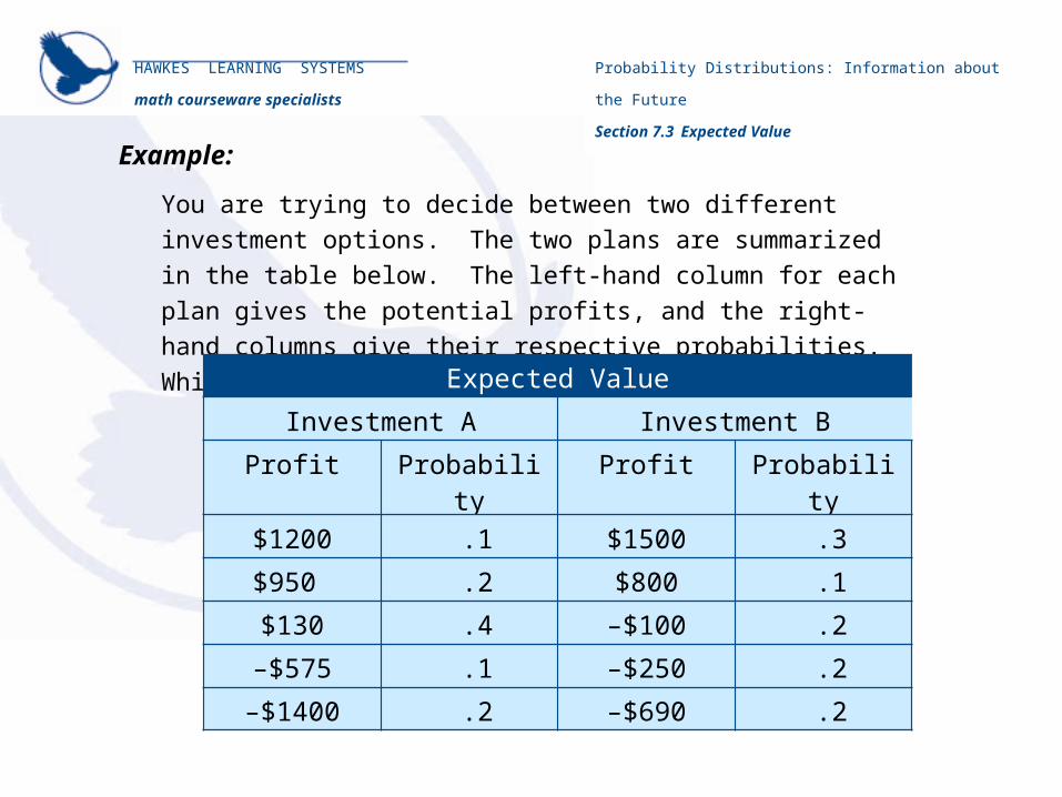
You are trying to decide between two different investment
options. The two plans are summarized in the table
below. The left-hand column for each plan gives the
potential profits, and the right-hand columns give their
respective probabilities. Which plan should you choose?
Example:
Expected Value
Investment A Investment B
Profit Probability Profit Probability
$1200 .1 $1500 .3
$950 .2 $800 .1
$130 .4 –$100 .2
–$575 .1 –$250 .2
–$1400 .2 –$690 .2
Probability Distributions: Information about the Future
Section 7.3 Expected Value
HAWKES LEARNING SYSTEMS
math courseware specialists
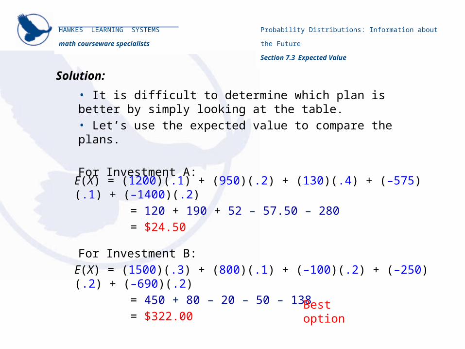
Solution:
• It is difficult to determine which plan is better by simply looking at the table. • Let’s use the expected value to compare the plans.
For Investment A:
For Investment B:
E(X) = (1200)(.1) + (950)(.2) + (130)(.4) + (–575)(.1) + (–1400)(.2)
= 120 + 190 + 52 – 57.50 – 280
= $24.50
E(X) = (1500)(.3) + (800)(.1) + (–100)(.2) + (–250)(.2) + (–690)(.2)
= 450 + 80 – 20 – 50 – 138
= $322.00 Best option
Probability Distributions: Information about the Future
Section 7.3 Expected Value

HAWKES LEARNING SYSTEMS
math courseware specialists
Probability Distributions: Information about the Future
Section 7.4 Variance of a Discrete Random Variable
Objectives:
• To define and describe the variance of a discrete random variable.
HAWKES LEARNING SYSTEMS
math courseware specialists
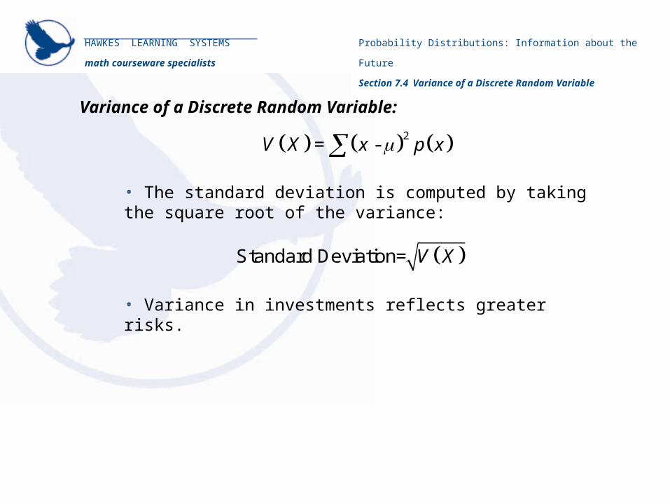
Variance of a Discrete Random Variable:
-V X x p x 2=
• The standard deviation is computed by taking the square root of the variance:
Standard Deviation= V X
• Variance in investments reflects greater risks.
Probability Distributions: Information about the Future
Section 7.4 Variance of a Discrete Random Variable

HAWKES LEARNING SYSTEMS
math courseware specialists
Variance of a Random Variable
Investment A Investment B
Profit Probability Profit Probability
$1200 .1 $1500 .3
$950 .2 $800 .1
$130 .4 –$100 .2
–$575 .1 –$250 .2
–$1400 .2 –$690 .2
To determine the risk, we need to calculate the variance of each investment.
Determine the Risk:
Probability Distributions: Information about the Future
Section 7.4 Variance of a Discrete Random Variable

HAWKES LEARNING SYSTEMS
math courseware specialists
Solution:For Investment A:
Variance of a Random Variable
Investment A
Profit Probability
$1200 .1
$950 .2
$130 .4
–$575 .1
–$1400 .2
-x p x 2
24.50A AE X
21200 24.50 0.1
2950 24.50 0.2
2130 24.50 0.4
2575 24.50 0.1
21400 24.50 0.2
138,180.03
171,310.05
4452.10
35,940.03
405,840.05
$755,722.26V X
Standard Deviation 755,722.24 $869.32V X
Probability Distributions: Information about the Future
Section 7.4 Variance of a Discrete Random Variable

HAWKES LEARNING SYSTEMS
math courseware specialists
Solution:
For Investment B:
Variance of a Random Variable
Investment B
Profit Probability
$1500 .3
$800 .1
–$100 .2
–$250 .2
–$690 .2
-x p x 2
322B BE X
21500 322 0.3
2800 322 0.1
2100 322 0.2
2250 322 0.2
2690 322 0.2
416,305.20
22,848.40
35,616.80
65,436.80
204,828.80
$745,036.00V X
Standard Deviation 745,036.00 $863.15V X
Probability Distributions: Information about the Future
Section 7.4 Variance of a Discrete Random Variable

HAWKES LEARNING SYSTEMS
math courseware specialists
Solution:
Since in terms of risk Investment B is considered the better option because it carries slightly less risk.
755,722.26 745,036.00 ,A BV X V X
Probability Distributions: Information about the Future
Section 7.4 Variance of a Discrete Random Variable
HAWKES LEARNING SYSTEMS
math courseware specialists
Probability Distributions: Information about the Future
Section 7.7 The Binomial Distribution
Objectives:
• To define a Binomial random variable.
• To calculate probabilities using the Binomial distribution.
• To calculate the expected value of a Binomial random variable.
• To calculate the variance of a Binomial random variable.

HAWKES LEARNING SYSTEMS
math courseware specialists
Definition:
• Binomial experiment – a random experiment which satisfies all of the following conditions.
i) There are only two outcomes on each trial of the experiment. (One of the outcomes is usually referred to as a success, and the other as a failure.)
ii) The experiment consists of n identical trials as described in Condition 1.
iii) The probability of success on any one trial is denoted by p and does not change from trial to trial. (Note that the probability of a failure is 1−p and also does not change from trial to trial.)
iv) The trials are independent.
v) The binomial random variable X is the count of the number of successes in n trials.
Probability Distributions: Information about the Future
Section 7.7 The Binomial Distribution
HAWKES LEARNING SYSTEMS
math courseware specialists
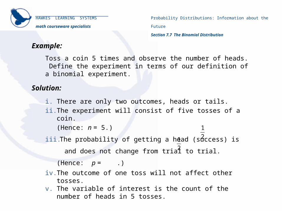
Toss a coin 5 times and observe the number of heads. Define the experiment in terms of our definition of a binomial experiment.
i. There are only two outcomes, heads or tails.
ii. The experiment will consist of five tosses of a coin.
(Hence: n = 5.)
iii. The probability of getting a head (success) is and does not
change from trial to trial. (Hence: p = .)
iv. The outcome of one toss will not affect other tosses.v. The variable of interest is the count of the number of heads in
5 tosses.
1
21
2
Probability Distributions: Information about the Future
Section 7.7 The Binomial Distribution
Example:
Solution:
HAWKES LEARNING SYSTEMS
math courseware specialists
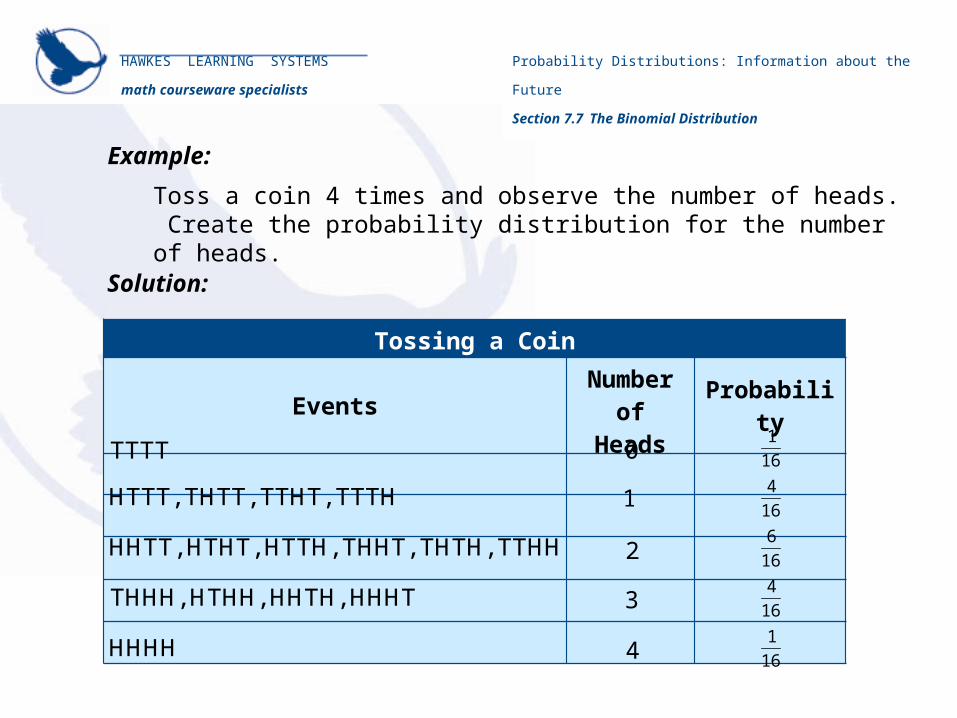
Toss a coin 4 times and observe the number of heads. Create the probability distribution for the number of heads.
Tossing a Coin
EventsNumber of Heads
Probability
HHTT, HTHT, HTTH, THHT, THTH, TTHH
TTTT
HTTT, THTT, TTHT, TTTH
THHH, HTHH, HHTH, HHHT
HHHH
0
1
2
3
4
1
16
4
16
6
16
4
16
1
16
Probability Distributions: Information about the Future
Section 7.7 The Binomial Distribution
Example:
Solution:

HAWKES LEARNING SYSTEMS
math courseware specialists
We will define the binomial probability distribution function as follows:
represents the number of combinations of n objects taken x at a time (without replacement) and is given by
!, where ! 1 2 ...1 and 0!=1.
! !nx
nC n n n n
x n x
1
n xn xxP X x C p p
where the number of trials,n
nxC
the number of successes, andx the probability of success.p
Probability Distributions: Information about the Future
Section 7.7 The Binomial Distribution
Binomial Probability Distribution Function:

What is the probability of getting exactly 7 tails in 18 coin
tosses?
Example:
HAWKES LEARNING SYSTEMS
math courseware specialists
Solution:
n = 18, p = .5, x = 7
1
n xn xxP X x C p p
7 18 7
187
1 17
21
2P X C
7 1118! 1 1
11!7! 2 2
Probability Distributions: Information about the Future
Section 7.7 The Binomial Distribution

A quality control expert at a large factory estimates that 10% of
all batteries produced are defective. If a sample of 20 batteries
are taken, what is the probability that no more than 3 are
defective?
Example:
HAWKES LEARNING SYSTEMS
math courseware specialists
Solution:
n = 20, p = .1, x = 3, but this time we need to look at the probability that no more than three are defective, which is
P(X ≤ 3).
0 1 33 2P X P X P X P X P X
0 20 1 1920 200 1
2 18 3 1720 202 3
0.1 0.9 0.1 0.9
0.1 0.9 0.1 0.9
C C
C C
0.867
Probability Distributions: Information about the Future
Section 7.7 The Binomial Distribution

HAWKES LEARNING SYSTEMS
math courseware specialists
Formulas:
Binomial expected value and variance can be defined with the following formulas.
E X np 1V X np p
Example:
A quality control expert at a large factory estimates that 10% of
all batteries produced are defective. If a sample of 20 batteries
is taken, what is the expected value, variance, and standard
deviation of the number of defective batteries?
Solution:
20, .1n p 20 0 2.1E X
120 0. 11 1 .80.V X
Standard Deviati 1.8on= 1.34V X
Probability Distributions: Information about the Future
Section 7.7 The Binomial Distribution

HAWKES LEARNING SYSTEMS
math courseware specialists
Probability Distributions: Information about the Future
Section 7.8 The Poisson Distribution
Objectives:
• To define a Poisson random variable.
• To calculate probabilities using the Poisson distribution.

HAWKES LEARNING SYSTEMS
math courseware specialists
Definitions:
• Poisson distribution – a discrete probability distribution that uses a fixed interval of time or space in which the number of successes are recorded.
where
• In the Poisson distribution
, for 0,1,2,...!
xeP X x x
x
2.71828..., and
average number of "successes".
e
.E X V X
Probability Distributions: Information about the Future
Section 7.8 The Poisson Distribution

1. The successes must occur one at a time.
2. Each success must be independent of any other successes.
HAWKES LEARNING SYSTEMS
math courseware specialists
Poisson Distribution Guidelines:
When calculating the Poisson distribution, round your answers to four decimal places.
Probability Distributions: Information about the Future
Section 7.8 The Poisson Distribution

Suppose that the dial-up Internet connection at your home goes
out an average of 0.75 times every hour. If you plan to be
connected to the internet for 3 hours one afternoon, what is the
probability that you will stay connected the entire time?
Assume that the dial-up disconnections follow a Poisson
distribution.
Example:
HAWKES LEARNING SYSTEMS
math courseware specialists
Solution:
x = 0, (0.75)(3) = 2.25
0.1054
Probability Distributions: Information about the Future
Section 7.8 The Poisson Distribution

A typist averages 1 typographical error per paragraph. If the
document has 4 paragraphs, what is the probability that there
will be less than 5 mistakes?
Example:
HAWKES LEARNING SYSTEMS
math courseware specialists
Solution:
x < 5, =This time we need to look at the probability that less than five mistakes will occur, which is P(X < 5).
(4)(1) = 4
P(X < 5) = P(X ≤ 4)
0.6288
Probability Distributions: Information about the Future
Section 7.8 The Poisson Distribution

A fast food restaurant averages 2 incorrect orders every 4 hours.
What is the probability that they will get at least 3 orders wrong in
any given day between 11 AM and 11PM? Assume that fast food
errors follow a Poisson distribution.
Example:
HAWKES LEARNING SYSTEMS
math courseware specialists
Solution:
x ≥ 3, =
This time we need to look at the probability that at least three wrong orders will occur, which is P(X ≥ 3).
(3)(2) = 6
P(X ≥ 3) = 1 – P(X < 3)
= 1 – P(X ≤ 2)
0.9380
Probability Distributions: Information about the Future
Section 7.8 The Poisson Distribution
! ! !
0 1 26 6 66 6 6
10 1 2
e e e
HAWKES LEARNING SYSTEMS
math courseware specialists
Objectives:
• To define a Hypergeometric random variable.
• To calculate probabilities using the Hypergeometric distribution.
• To calculate the expected value of a Hypergeometric random
variable.
• To calculate the variance of a Hypergeometric random variable.
Probability Distributions: Information about the Future
Section 7.9 The Hypergeometric Distribution

• Hypergeometric distribution – a special discrete probability function for problems with a fixed number of dependent trials and a specified number of countable successes.
HAWKES LEARNING SYSTEMS
math courseware specialists
Definitions:
• When calculating the hypergeometric distribution, round your answers to four decimal places.
, where 0 min ,A N Ax n x
Nn
C CP X x x A n
C
the total number of successes possibleA the size of the population, andN the size of the sample drawn.n
Probability Distributions: Information about the Future
Section 7.9 The Hypergeometric Distribution
1. Each trial consists of selecting one of the N items in the population and results in either a success or a failure.
2. The experiment consists of n trials.
3. The total number of possible successes in the entire population is A.
4. The trials are dependent. (i.e., selections are made without replacement.)
HAWKES LEARNING SYSTEMS
math courseware specialists
Hypergeometric Distribution Guidelines:
Probability Distributions: Information about the Future
Section 7.9 The Hypergeometric Distribution

At the local grocery store there are 50 boxes of cereal on the
shelf, half of which contain a prize. Suppose you buy 4 boxes
of cereal. What is the probability that 3 boxes contain a prize?
Example:
HAWKES LEARNING SYSTEMS
math courseware specialists
A = 25, x = 3, N = 50, n = 4
25 50 253 4 3
504
3C C
P XC
25 253 1
504
C C
C
2300 25
2303000.2497
Probability Distributions: Information about the Future
Section 7.9 The Hypergeometric Distribution
Solution:

HAWKES LEARNING SYSTEMS
math courseware specialists
A produce distributor is carrying 10 boxes of Granny Smith apples
and 8 boxes of Golden Delicious apples. If 6 boxes are randomly
delivered to one local market, what is the probability that at least 4
of the boxes delivered contain Golden Delicious apples?
Example:
Solution:
A = 8, x ≥ 4, N = 18, n = 6
4 5 64P X P X P X P X 8 18 8 8 18 8 8 18 84 6 4 5 6 5 6 6 6
18 18 186 6 6
C C C C C C
C C C
70 45 56 10 28 1
18564 18564 18564
0.2014
Probability Distributions: Information about the Future
Section 7.9 The Hypergeometric Distribution

HAWKES LEARNING SYSTEMS
math courseware specialists
Formulas:
Hypergeometric expected value and variance can be defined with the following formulas.
AE X n
N
11
N nA AV X n
N N N
Probability Distributions: Information about the Future
Section 7.9 The Hypergeometric Distribution

HAWKES LEARNING SYSTEMS
math courseware specialists
Example:
A produce distributor is carrying 10 boxes of Granny Smith apples and 8 boxes of Golden Delicious apples. If 6 boxes are randomly delivered to one local market, what is the expected value and variance of the distribution?
Solution:
A = 8, N = 18, n = 6
E X8
618
8
3
V X 18 68 8
618 18 18
11
160
153
Probability Distributions: Information about the Future
Section 7.9 The Hypergeometric Distribution