harmonics propagation and impact of electric vehicles on ...753273/fulltext01.pdf · harmonics...
TRANSCRIPT
Harmonics propagation and impact of Electric Vehicles on
the electrical grid Master thesis report
Kevin LORENZO
07/02/2014
Supervisor : Staffan NORRGA EJ211X Degree Project in Power Electronics
EDF R&D Clamart KTH - Stockholm
Master Thesis Report Harmonics propagation and impact of EVs on the grid
Kévin LORENZO
1
Abstract
This thesis addresses the issues of (inter)harmonics propagation on electrical grids. More
specifically it concerns two different kinds of studies. The first one is the harmonic impact of the
integration of new technologies such as Electric Vehicle charging parks which generate
harmonic voltages. The second one is the propagation on these grids of communication signals
such as the pricing signal. These two kinds of voltages behave a priori the same way since they
are superimposed to the fundamental feeding voltage, with a higher frequency. However, their
main structural difference is that, while harmonic voltages generated by electric cars are
unwanted on electrical grid, the pricing signal is intended at certain points of the grid.
For the first kind of studies, concerning harmonics generated by Electric Vehicles, the aim of this
project was to determine the problems that may appear on electrical grids when electric car
parks are connected thereto. To do so, laboratory measurements on several Electric Vehicle
models, separately or simultaneously, were performed. From their results, different models of
EVs have been drawn up enabling to perform simulations on an existing car park. Some
measurements were then carried out on this car park in order to conclude on its impact on the
Power Quality of the grid.
The second study is about the pricing signal propagation. It focuses on different ways of
modeling grid components, especially loads, in simulation tools at the specific frequency of this
signal. For Medium Voltage grids, several load models can be found in the literature and are
compared in this report. For Low Voltage grids, a model based on the results of recent
measurements is suggested in the report.

EDF R&D Clamart KTH - Stockholm
Master Thesis Report Harmonics propagation and impact of EVs on the grid
Kévin LORENZO
2
Acknowledgment
First of all, I would like to thank my supervisor in KTH, Staffan Norrga, for giving me the
opportunity to do this master thesis and for his support during the project.
I would like to express my deepest gratitude to my supervisor in EDF, Géraud Rias, for his
guidance through this degree project, his advice and his great support.
I would also like to thank the whole Power Quality group of EDF R&D for having warmly
welcomed me in the group. Within this group, I address a special thank to Ludovic Bertin for the
time he spent answering my question and his encouragements.

EDF R&D Clamart KTH - Stockholm
Master Thesis Report Harmonics propagation and impact of EVs on the grid
Kévin LORENZO
3
Table of contents Abstract .................................................................................................................................................................................. 1
Acknowledgment ............................................................................................................................................................... 2
List of abbreviations ......................................................................................................................................................... 5
List of figures and tables ................................................................................................................................................. 6
I. Introduction ................................................................................................................................................................ 8
1.1. The company EDF R&D and its Power Quality group...................................................................... 8
1.2. Background ....................................................................................................................................................... 8
1.3. Objectives ........................................................................................................................................................... 9
1.4. Overview of the thesis .................................................................................................................................. 9
II. Presentation of the field ..................................................................................................................................... 11
2.1. Theoretical background on harmonics ............................................................................................... 11
2.1.1. General definitions ............................................................................................................................ 11
2.1.2. Origins..................................................................................................................................................... 14
2.1.3. Propagation .......................................................................................................................................... 15
2.1.4. Effects ...................................................................................................................................................... 15
2.1.5. Standards ............................................................................................................................................... 16
2.2. Harmonic measurements ......................................................................................................................... 16
2.3. Harmonics emission of Electrical Vehicles........................................................................................ 17
2.4. Modeling of harmonics propagation .................................................................................................... 18
2.4.1. Assessing the harmonic impedance of a grid ......................................................................... 19
2.4.2. Harmonic modeling of grid components .................................................................................. 20
2.5. Ripple control signal propagation ........................................................................................................ 24
2.5.1. Ripple Control Signal ........................................................................................................................ 24
2.5.2. Load modeling under RCS .............................................................................................................. 25
III. Study of EVs harmonic behavior and modeling ................................................................................... 26
3.1. Unit testing on existing cars .................................................................................................................... 26
3.1.1. Unit testing process ........................................................................................................................... 26
3.1.2. Results of measurements: Harmonic behavior of EVs ........................................................ 27
3.1.3. EV behavior at higher frequencies .............................................................................................. 32
3.2. Multiple testing on 4 EVs .......................................................................................................................... 34
3.3. Simplified harmonic model ..................................................................................................................... 37
3.4. Possible extensions of the harmonic model ..................................................................................... 39
IV. Case study 1: An existing car park of 10 Electric Vehicles .............................................................. 41
EDF R&D Clamart KTH - Stockholm
Master Thesis Report Harmonics propagation and impact of EVs on the grid
Kévin LORENZO
4
4.1. Background .................................................................................................................................................... 41
4.2. Modeling of the car park ........................................................................................................................... 42
4.3. Results of simulation .................................................................................................................................. 43
4.4. Measurements campaign .......................................................................................................................... 45
4.4.1. Method and measurement devices ............................................................................................. 45
4.4.2. Measurement results ........................................................................................................................ 46
4.4.3. Observation: Behavior at higher frequencies ......................................................................... 49
4.5. Discussion ....................................................................................................................................................... 51
V. Case study 2: Load modeling under Ripple Control signal .................................................................. 53
5.1. Background .................................................................................................................................................... 53
5.2. Load models comparison at MV ............................................................................................................ 53
5.3. From MV model to LV model .................................................................................................................. 59
5.4. Grid reduction ............................................................................................................................................... 63
5.5. Discussion ....................................................................................................................................................... 65
VI. Conclusion ........................................................................................................................................................... 66
References .......................................................................................................................................................................... 67
Appendices ........................................................................................................................................................................ 68
Appendix 1: International standard IEC 61000-3-2 on harmonic currents emission ................... 68
Appendix 2: European standard EN50160 on harmonic voltages emission ..................................... 69
EDF R&D Clamart KTH - Stockholm
Master Thesis Report Harmonics propagation and impact of EVs on the grid
Kévin LORENZO
5
List of abbreviations
CB: Circuit Breaker
EV: Electric Vehicle
GTO: Gate Turn-Off
HF: High Frequency
HV: High Voltage
LV: Low Voltage
MV: Medium Voltage
PCC: Point of Common Coupling
PCSC: Point of Charging Stations Connection
PLC: Power Line Carrier
PWM: Pulse Width Modulation
R&D: Research and Development
RCS: Ripple Control Signal
RMS: Root Mean Square
THC: Total Harmonic Current
THD: Total Harmonic Distortion
EDF R&D Clamart KTH - Stockholm
Master Thesis Report Harmonics propagation and impact of EVs on the grid
Kévin LORENZO
6
List of figures and tables
Figure 1: Influence of third and fifth harmonic on a sinusoidal wave ................................................................... 12
Figure 2: Equivalent circuit of a grid seen from point A, at the harmonic rank h ................................................. 13
Figure 3 : Diode rectifier scheme and input current waveform ............................................................................. 14
Figure 4 : Harmonic current, impedance and voltage ........................................................................................... 14
Figure 5 : Harmonics propagation on the grid ...................................................................................................... 15
Figure 6 : Mode 3 of charging [9] .......................................................................................................................... 18
Figure 7 : Block diagram: General topology of an EV charging system ................................................................ 18
Figure 8: Pi-Equivalent model of lines/cables........................................................................................................ 21
Figure 9 : General MV grid modeling .................................................................................................................... 24
Figure 10 : Ripple Control Signal Injection............................................................................................................. 25
Figure 11 : Unit testing layout ............................................................................................................................... 27
Figure 12 : Data acquisition system ...................................................................................................................... 27
Figure 13 : Example of an electric vehicle (EV1) charging cycle ............................................................................ 28
Figure 14 : EV1 current waveform during the “main charging” phase ................................................................. 29
Figure 15 : EV1 current waveform during the “end of charging” phase ............................................................... 29
Figure 16 : Mean current spectrum for EV1 .......................................................................................................... 30
Figure 17 : Maximum current spectrum for EV1 during the charging cycle .......................................................... 31
Figure 18 : Mean current spectrum for EV2 .......................................................................................................... 31
Figure 19 : Temporal evolution of the current harmonic distortion during the charging cycle ............................. 32
Figure 20 : Current spectrum for EV1 in the range [2 - 150 kHz] ........................................................................... 33
Figure 21 : Voltage spectrum for EV1 in the range [2 - 150 kHz] .......................................................................... 34
Figure 22 : Multiple testing layout ........................................................................................................................ 35
Figure 23 : Harmonic spectrum for the "Low grid impedance" test ...................................................................... 36
Figure 24 : Harmonic spectrum for the "Reference impedance" test .................................................................... 36
Figure 25 : Simple model of an electric vehicle ..................................................................................................... 37
Figure 26 : Current phase spectrum of EV1 ........................................................................................................... 38
Figure 27 : Inverse Fourier transform of EV1's model ........................................................................................... 38
Figure 28 : Inverse Fourier transform of "3-2 standard" model ............................................................................ 39
Figure 29 : Car park with 10 charging stations for EVs ......................................................................................... 41
Figure 30 : Simulation circuit of the electric car park ............................................................................................ 42
Figure 31 : Mean voltage spectrum at the point of charging stations connection for 10 EV1 .............................. 44
Figure 32 : Mean voltage spectrum at the point of common coupling for 10 EV1 ................................................ 44
Figure 33 : Mean voltage spectrum at the point of common coupling for "Ten 3-2 standard" configuration ...... 45
Figure 34 : Data acquisition system at the PCC (Main Low Voltage Board) .......................................................... 46
Figure 35 : Temporal evolution of voltage THD and current absorbed by phase 1 ............................................... 47
Figure 36 : Influence of EV1 connection on the mean voltage spectrum .............................................................. 48
Figure 37 : Influence of EV3 connection on the mean voltage spectrum .............................................................. 49
Figure 38 : One mean voltage spectrum every hour over 24h .............................................................................. 50
Figure 39 : Illustration of perturbations variations in a 30s period ....................................................................... 51
Figure 40 : Simple MV grid with RCS injection (50 Hz and 175 Hz) ....................................................................... 54
Figure 41 : Comparison of equivalent impedance magnitudes of each of the first three models ......................... 55
Figure 42 : Comparison of equivalent impedance magnitudes of each of the last three models ......................... 56
Figure 43 : Comparison of the most favorable and the less favorable models on average .................................. 56
Figure 44 : Simulation grid for models comparison .............................................................................................. 57
Figure 45 : Comparison of RCS rates for each of the models, with and without capacitor bank .......................... 58

EDF R&D Clamart KTH - Stockholm
Master Thesis Report Harmonics propagation and impact of EVs on the grid
Kévin LORENZO
7
Figure 46 : "LV Model" of a typical aggregate load .............................................................................................. 59
Figure 47 : Magnitudes comparison for "LV model" and "Measurements model" (d=0.5) ................................... 61
Figure 48 : Magnitudes comparison for "LV model" and "Measurements model" (Optimized d) ........................ 62
Figure 49 : , magnitudes comparison for "LV model" and "Measurements model" (Optimized d) ... 62
Figure 50: Argument of the adjusted "LV model" equivalent impedance ............................................................. 63
Figure 51 : Equivalence between detailed network and aggregate one (same model and cables impedance
neglected).............................................................................................................................................................. 64
Table 1: Levels of voltage distortion causing effects on equipments ___________________________________ 15
Table 2 : Harmonic impedance assessment methods _______________________________________________ 19
Table 3: Electric vehicles caracteristics __________________________________________________________ 28
Table 4 : Total Harmonic Distortions for the simulation ____________________________________________ 43
Table 5 : Total Harmonic Distortion for each configuration __________________________________________ 47
EDF R&D Clamart KTH - Stockholm
Master Thesis Report Harmonics propagation and impact of EVs on the grid
Kévin LORENZO
8
I. Introduction
1.1. The company EDF R&D and its Power Quality group
EDF, which stands for “Electricité De France”, is a French electric utility company. Its 640 TWh of
electric energy generated in 2012 make EDF the world’s largest producer of electricity. With its
subsidiaries such as ERDF, in charge of electricity distribution, and RTE in charge of the
transmission grid, the group is present within all sectors of electricity. EDF develops its activities
mainly in Western Europe, but also in Brazil, United State or China through different
subsidiaries. In total, EDF has 160,000 employees for 39 M of customers. The turnover was
€73 Bn in 2012, and the R&D budget was €523 M [1].
EDF R&D employs around 1700 researchers in 15 different departments. One of these
departments is called “MIRE” which stands for Measurement and Information System of
Electrical Grids. This department mainly carries out studies about the future of electrical grids,
for transmission system as well as distribution system. Within this department, the “Power
Quality group” performs technical studies, develops materials and simulation tools, and
participates in normalization activities concerning power quality on the grid.
This thesis was done in this group, and concerned one of its main activities, which is to study the
quality of the supplied voltage and the impact of new applications on electrical grids such as
Electric Vehicles.
1.2. Background
The relatively recent development of power electronic components has had a massive
contribution to the progress in all electricity applications. The thyristors, GTO or high power
transistors for example have brought an important improvement in electrical circuits’ control
and flexibility in use. These improvements concern a lot of applications, from power converters
to micro-computers. However, these power electronic technologies may have some negative
effects, such as the creation of perturbations in voltage and current waves. These effects, and
more particularly the creation of harmonics currents and voltages, are the price for the fast
improvement in power electronics.
The Power Quality group at EDF R&D carries out more and more studies in order to apprehend
harmonic perturbations. These studies concern all kind of power electronics applications, but a
focus has been recently set on Electric Vehicles (EVs). Indeed, since EVs are being used more
and more, the study of the effect of their charging on the local grid seems essential. Thus, the
first part of this thesis will focus on the impact of the charging of EVs on the Power Quality of the
distribution electrical grid.
The second part of this thesis concerns a more general study about the propagation of
harmonics on a grid. More specifically, it relates to the modeling of harmonic behavior of
different grid components. Indeed, if one wants to be able to develop simulation tools to study
harmonics and interharmonics propagation, some models representing grid components such as
cables, transformers and all kind of loads are necessary.

EDF R&D Clamart KTH - Stockholm
Master Thesis Report Harmonics propagation and impact of EVs on the grid
Kévin LORENZO
9
As the assessment of harmonic impedances on a grid is not an easy problem to deal with, the
models that are today used in simulation tools mostly depend either on experimental results
from measurement campaigns or on assumptions on the grid structure. It is thus essential to
study these models, to be able to better understand the propagation of unintended harmonic
perturbations as well as intended communication signals.
In this part of the thesis, a focus will be put on the modeling of large loads on the grid, and
especially their behavior to the Ripple Control Signal, which is used on French distribution grid
as a way to transmit tariff orders to customer installations.
1.3. Objectives
The main objective of the first part of this thesis is to study the harmonic perturbations that an
electric car park can produce on the surrounding Low Voltage electrical grid when several
vehicles are charging. To do so, the aim is first to characterize the harmonic behavior of some
electric vehicles, by performing and analyzing measures on several vehicles in a laboratory.
From this, a typical model for each vehicle tested needs to be found, in order to be able to
simulate various grids containing EV charging stations.
The models found from the previous step are used to carry out simulations of existing grids
containing electric vehicle charging stations. The aim then is to compare simulations of a specific
site to measurements performed on the same site. This done, an analysis of both kinds of study
allows to determine whether an electric car park might disturb the surrounding grid or if
harmonic problems are unlikely to happen on the grid when vehicles are connected.
The aim of the second part of this thesis is to study the propagation of one particular kind of
signal: the Ripple Control Signal. This signal is a 175 Hz voltage signal superimposed at MV-
substations whose fundamental frequency is, in Europe, 50 Hz.
First, as several models can be found in the literature to represent harmonic loads on MV grids,
the aim will be to understand the impact of using one model or another on the study of Ripple
Control Signal (RCS) propagation. So, it consists in making use of the models at one particular
frequency (175 Hz) and comparing the results that it would give in terms of RCS propagation on
MV distribution grids.
Then, the aim will be to suggest and adjust one model in order to make it fit with recent
measurements on MV/LV substations.
Also, the problem of grid reduction will be discussed. Indeed, one of the objectives will be to
determine if it is better to use, in simulation tools, a single model of large load which represents
the aggregation of all loads connected to a point of the MV grid, or if it is better to model
separately each of the MV loads and thus keep a detailed grid.
1.4. Overview of the thesis

EDF R&D Clamart KTH - Stockholm
Master Thesis Report Harmonics propagation and impact of EVs on the grid
Kévin LORENZO
10
This report is divided in four main sections. The first one presents the field of Power quality and
provides the necessary theoretical background. The focus is put on introducing the concept of
harmonics, their origins, effects, propagation. Their generation in electric vehicles and the ways
how to model their propagation are also discussed.
The second part presents a study of EVs harmonic behavior. This section describes the results of
unit testing as well as multiple testing on electric vehicles, in order to characterize their
behavior in terms of harmonics generation and to be able to develop simulation models.
The third section is a case study which describes the impact of an existing car park on the
distribution network by two kinds of studies: simulations and measurements.
The fourth one concerns the propagation of a particular interharmonic signal on the distribution
grid, and more specifically the modeling of grid components at this signal’s frequency.
EDF R&D Clamart KTH - Stockholm
Master Thesis Report Harmonics propagation and impact of EVs on the grid
Kévin LORENZO
11
(Eq. 1)
(Eq. 2)
(Eq. 3,4)
(Eq. 5)
(Eq. 6,7)
(Eq. 8)
II. Presentation of the field
2.1. Theoretical background on harmonics
2.1.1. General definitions
Harmonics appear on the current wave as well as on the voltage wave. They are permanent
perturbations of these waves due to non-linear charges or irregularities in electrotechnical
equipment for example. Their frequencies are multiple of the fundamental frequency.
Indeed, according to Fourier’s theory, every periodic signal can be seen as a sum of a steady
signal and sinusoidal signals: one with a chosen fundamental frequency and the other ones with
frequencies which are multiple of this fundamental one. Taking s(t) as a T-periodic signal (with
frequency and pulsation ), it can be written as:
( ) ∑( ( ) ( ))
With
∫ ( )
And for
∫ ( ) ( )
and
∫ ( ) ( )
It can also be written as:
( ) ∑ ( )
Where √
and (
)
Considering the fact that most of electrical quantities are intended to be sinusoidal, the electrical
signals can be seen as their fundamental component, which is an ideal perfectly sinusoidal
signal, and a sum of harmonics which represents the perturbations of this signal. The
fundamental frequency can be or depending on the place where it is used,
and the frequency of a harmonic of rank is then ( is an integer):
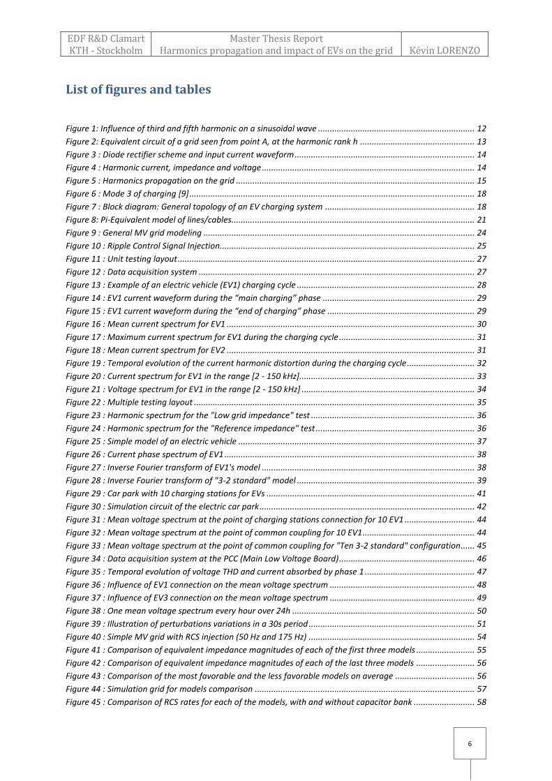
The following figure shows an example of how a sinusoidal signal with an arbitrary magnitude of
100, is distorted by two of its harmonics of rank 3 and 5 with magnitudes of 20 and 10
respectively and no phase angle.

EDF R&D Clamart KTH - Stockholm
Master Thesis Report Harmonics propagation and impact of EVs on the grid
Kévin LORENZO
12
(Eq. 9)
(Eq. 10)
(Eq. 11)
Figure 1: Influence of third and fifth harmonic on a sinusoidal wave
What is called magnitude of the harmonic of rank h is actually the RMS value of its sinusoid,
given by:
√
The phase angle of the harmonic of rank h is .
It has to be noted that the RMS value of a harmonically distorted signal is different than the RMS
value of its fundamental. Indeed, for a distorted current for example, the RMS value is the
quadratic sum of the RMS value of all harmonic ranks, taking the fundamental into account.
√∑
With a 50 Hz fundamental frequency, the perturbations are called harmonics when they are in
the range of frequency [100 Hz - 2 kHz], so from the 2nd and up to the 40th rank. Above this rank,
they are no more harmonics, but are here called “high frequency perturbations”.
A way to characterize the harmonic distortion of a signal is to use the so called THD (Total
Harmonic Distortion). It gives an information on the whole harmonic content in the range
[100 Hz - 2 kHz], and can be defined [2] both in voltage and in current as:
√∑ (
)
√∑ (
)
Where (respectively ) is the magnitude of the harmonic current (respectively voltage). The
THD is usually expressed in %.

EDF R&D Clamart KTH - Stockholm
Master Thesis Report Harmonics propagation and impact of EVs on the grid
Kévin LORENZO
13
(Eq. 12)
(Eq. 13)
To get an idea of which part of the actual RMS current is contained in the harmonics, one can
define the “total harmonic current” (THC), which is a quadratic sum of each harmonic
contribution to the current [2] and is given by:
√∑
Finally, with these definitions, the RMS value of the current is given by:
√ √
( )
This enables to understand that, the higher the THD, the bigger the RMS current, and thereby the
higher the heating of equipments for example.
The notions presented until now only take into account harmonics, and not interharmonics.
These latter can be defined in the same way as harmonics, but with h not being an integer. Thus,
their frequencies are not multiple of the fundamental one. For instance, with a 50 Hz
fundamental frequency, an interharmonic current can be calculated for the rank 3.5 (frequency
175 Hz).
By convention [2], the non-linear charges are consuming a current with a 50 Hz frequency in
Europe. As this current is distorted, these charges are said to be emitter of harmonic current,
towards the grid. Non-linear charges can thus be called harmonic current injectors.
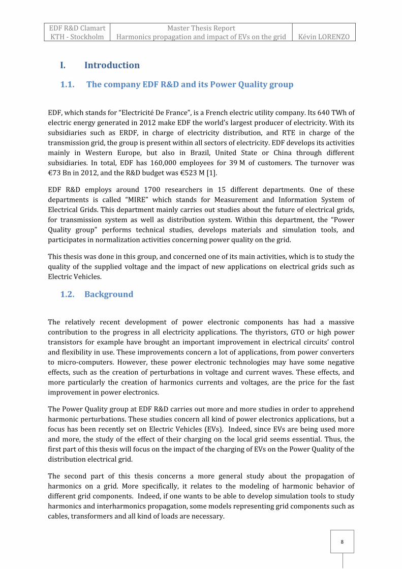
For each point of a given grid, since the impedance depends on the frequency at which it is
considered, a harmonic impedance can be defined. This actually represents the impedance of
every line converging to this point in parallel. The figure below represent a simple grid with
disturbing and non-disturbing charges and its equivalent circuit seen from point A, for the
harmonic rank h. takes into account the impedance of the non-disturbing charge but also the
disturbing one at this frequency, and the upstream grid.
Figure 2: Equivalent circuit of a grid seen from point A, at the harmonic rank h
EDF R&D Clamart KTH - Stockholm
Master Thesis Report Harmonics propagation and impact of EVs on the grid
Kévin LORENZO
14
(Eq. 14)
Thereby, some harmonic voltages are created at each point of the grid, and are given by:
2.1.2. Origins
There are two main kinds of harmonics: the harmonics coming from energy production, and the
ones coming from non-linear charges. The first ones, which are a bit less significant than the
others, are mainly due to imperfections of rotating machines (very low [2]) and decentralized
energy producers connected to the grid through power electronics. Non-linear charges can be
asynchronous motors, electrical lighting, electric arc furnaces[3] and all kind of power
electronics through which charges are connected.
In this second case, a non-linear charge absorbs non-sinusoidal current and thus emits harmonic
currents, which themselves turn to harmonic voltages. These harmonic voltages depend on the
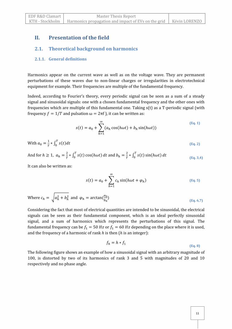
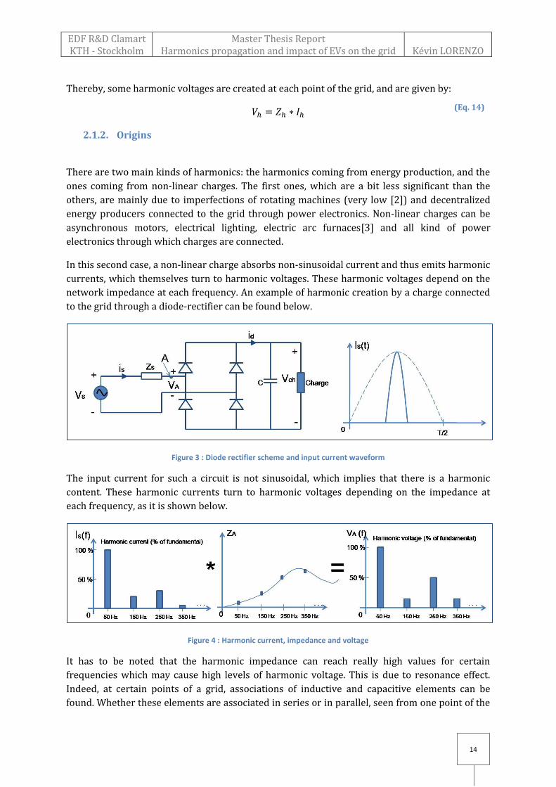
network impedance at each frequency. An example of harmonic creation by a charge connected
to the grid through a diode-rectifier can be found below.
Figure 3 : Diode rectifier scheme and input current waveform
The input current for such a circuit is not sinusoidal, which implies that there is a harmonic
content. These harmonic currents turn to harmonic voltages depending on the impedance at
each frequency, as it is shown below.
Figure 4 : Harmonic current, impedance and voltage
It has to be noted that the harmonic impedance can reach really high values for certain
frequencies which may cause high levels of harmonic voltage. This is due to resonance effect.
Indeed, at certain points of a grid, associations of inductive and capacitive elements can be
found. Whether these elements are associated in series or in parallel, seen from one point of the
EDF R&D Clamart KTH - Stockholm
Master Thesis Report Harmonics propagation and impact of EVs on the grid
Kévin LORENZO
15
(Eq. 15)
grid, they may lead to two kinds of resonance: parallel and series. While a series resonance
lower down the equivalent impedance close to the resonance frequency, a parallel resonance
increase it. For both kinds of resonance, the resonance frequency is given by:
√
This resonance phenomenon can be a serious problem on the grid, since bank capacitors
connected at substations are often used in order to compensate reactive power for example.
Cables and overhead lines also have a capacitive component.
2.1.3. Propagation
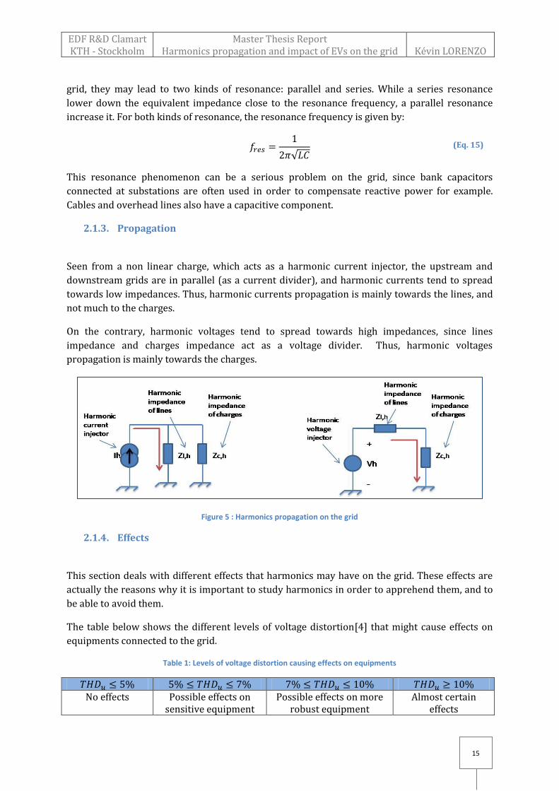
Seen from a non linear charge, which acts as a harmonic current injector, the upstream and
downstream grids are in parallel (as a current divider), and harmonic currents tend to spread
towards low impedances. Thus, harmonic currents propagation is mainly towards the lines, and
not much to the charges.
On the contrary, harmonic voltages tend to spread towards high impedances, since lines
impedance and charges impedance act as a voltage divider. Thus, harmonic voltages
propagation is mainly towards the charges.
Figure 5 : Harmonics propagation on the grid
2.1.4. Effects
This section deals with different effects that harmonics may have on the grid. These effects are
actually the reasons why it is important to study harmonics in order to apprehend them, and to
be able to avoid them.
The table below shows the different levels of voltage distortion[4] that might cause effects on
equipments connected to the grid.
Table 1: Levels of voltage distortion causing effects on equipments
No effects Possible effects on
sensitive equipment Possible effects on more
robust equipment Almost certain
effects
EDF R&D Clamart KTH - Stockholm
Master Thesis Report Harmonics propagation and impact of EVs on the grid
Kévin LORENZO
16
(Eq. 16)
Two kinds of effects appear on the grid: instantaneous effects and long-term effects. Some of the
most common instantaneous effects are problems with control circuits, relays and breakers
operation. More generally, some troubles may appear with all kinds of equipment that use zero
crossing as reference. Indeed, if an originally sinusoidal signal is distorted enough, it can cross
the zero reference several times during half a period.
Concerning long term effects, harmonics can cause ageing of components, mostly due to
overheating of transformers, motors and cables. Also, due to resonance phenomena which have
been previously introduced, harmonics can cause the destruction of capacitors on the grid which
are usually used to compensate reactive power.
2.1.5. Standards
When studying harmonics, it is really important to have an idea on which European or global
standards limit harmonic emissions on the grid. To do so, the kind of equipment which is studied
and the voltage level of the grid it is connected to, have to be defined.
In this thesis, the main equipment concerned is electric vehicles. The EVs that are studied and
modeled later on are all connected to the low voltage grid through a single phase station, and
absorb a current below 16 A. Thus, the standard that can be applied on these EVs is the
international standard “IEC 61000-3-2” for Class A equipment which limits the emissions of
harmonic currents for devices such as EVs connected to the low voltage grid and absorbing less
than 16 A (RMS value) [5]. The limits of harmonic current emissions for each harmonic rank in
the frequency range 100 Hz to 2 kHz are given in a table extracted from the standard in
Appendix 1.
Concerning harmonic voltages, the standard which defines the limits that must not be exceeded
on the low voltage grid is the European standard EN50160 [6]. A table with these limits can be
found in Appendix 2.
2.2. Harmonic measurements
There are different methods to measure a harmonic spectrum at one point of the electrical grid.
Concerning the current wave, a general method, which is inspired by the one described in the
standard IEC 61000-3-2 mentioned above, is presented here.
In order to get a current harmonic spectrum, the current waveform is first measured and
recorded with a certain sampling frequency . Then, a Discrete Fourier Transform (DFT) is
applied to each 200 ms interval of this signal. The number of points of these intervals is
. The equation below gives the value of the harmonic current of rank k obtained by a
DFT. represents the nth current value in the 200ms interval.
∑
EDF R&D Clamart KTH - Stockholm
Master Thesis Report Harmonics propagation and impact of EVs on the grid
Kévin LORENZO
17
(Eq. 17)
At a 50 Hz frequency, 200 ms represent 10 periods of the current waveform. Thus, the DFT
gives a magnitude for each (inter)harmonic with a 5 Hz step. This means that, for each 200 ms-
long interval of the recorded signal, a spectrum is obtained with the values of , , and so
on until corresponding to the 40th rank.
Then, if the aim is to compare the harmonic spectrum to the standard limits, a grouping of
interharmonic magnitudes needs to be done, by calculating a quadratic sum of each
interharmonic component from to to obtain the magnitude of rank h. For
the boundary values, only half of their energy is kept, and the final equation is (for h>2) [7]:
√
But if the aim is to investigate certain harmonic frequencies, then no grouping needs to be done
and only fundamental and harmonic values can be picked. The magnitude and phase of each of
these values are kept for studies. Thus, the spectrum values, for , are:
In this thesis, the aim is to investigate harmonic behaviors, so the second method was used. After
this step, a harmonic spectrum is obtained every 200 ms, and an arithmetic mean can be
computed on a 2min30s period, representative of a certain behavior of the equipment that is
studied. This period usually corresponds to the one where harmonic distortion is the highest.
Thereby, a “mean spectrum” is obtained.
Once again, if the aim is to compare the spectrum with the standard, another data processing
needs to be done. Indeed, before the calculation of the mean spectrum, a smoothing filter with a
1.5 s time constant must be applied in order to smooth the evolution of each harmonic
magnitude. However, this thesis focuses on investigating harmonic phenomena, and not
checking the compliance to the standards. This is why no smoothing will be done later on.
The same method is used in order to obtain a voltage harmonic spectrum, except that the mean
spectrum is usually computed on a 10 min period.
2.3. Harmonics emission of Electrical Vehicles
In order to understand why the current absorbed by an EV connected to the grid is not perfectly
sinusoidal, this section briefly describes a general topology of an electric vehicle charging
system.
The charging process of an electrical vehicle is controlled by what is usually called Battery
Management System (BMS). The latter allows the battery to be charged, without being
overheated or overloaded for example. The most common charging method is certainly the
“Constant Current Constant Voltage” method, which means that, during the principal phase of
the charging process, the current is controlled to be maintained constant, and when the State of
Charge reaches a certain value, it is the voltage that is controlled to be constant. However, other
charging methods exist and are used, even though less commonly [8].
EDF R&D Clamart KTH - Stockholm
Master Thesis Report Harmonics propagation and impact of EVs on the grid
Kévin LORENZO
18
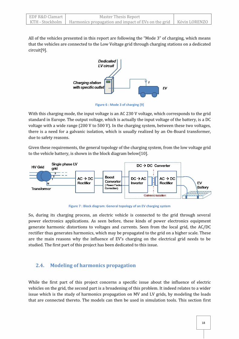
All of the vehicles presented in this report are following the “Mode 3” of charging, which means
that the vehicles are connected to the Low Voltage grid through charging stations on a dedicated
circuit[9].
Figure 6 : Mode 3 of charging [9]
With this charging mode, the input voltage is an AC 230 V voltage, which corresponds to the grid
standard in Europe. The output voltage, which is actually the input voltage of the battery, is a DC
voltage with a wide range (200 V to 500 V). In the charging system, between these two voltages,
there is a need for a galvanic isolation, which is usually realized by an On-Board transformer,
due to safety reasons.
Given these requirements, the general topology of the charging system, from the low voltage grid
to the vehicle battery, is shown in the block diagram below[10].
Figure 7 : Block diagram: General topology of an EV charging system
So, during its charging process, an electric vehicle is connected to the grid through several
power electronics applications. As seen before, these kinds of power electronics equipment
generate harmonic distortions to voltages and currents. Seen from the local grid, the AC/DC
rectifier thus generates harmonics, which may be propagated to the grid on a higher scale. These
are the main reasons why the influence of EV’s charging on the electrical grid needs to be
studied. The first part of this project has been dedicated to this issue.
2.4. Modeling of harmonics propagation
While the first part of this project concerns a specific issue about the influence of electric
vehicles on the grid, the second part is a broadening of this problem. It indeed relates to a wider
issue which is the study of harmonics propagation on MV and LV grids, by modeling the loads
that are connected thereto. The models can then be used in simulation tools. This section first

EDF R&D Clamart KTH - Stockholm
Master Thesis Report Harmonics propagation and impact of EVs on the grid
Kévin LORENZO
19
(Eq. 18)
(Eq. 19)
(Eq. 20)
presents the ways how to assess the harmonic impedance at one point of grid, and then derive a
model of the loads connected to the grid. This relates to the general problem of grid reduction.
2.4.1. Assessing the harmonic impedance of a grid
Since non-linear charges are usually considered as harmonic currents injectors [2], it is
important to be able to assess the harmonic impedance of the network in order to calculate the
harmonic voltages resulting from this injection. There is no universal method [11] to assess the
harmonic impedance of the network but a general one is presented below.
The basic principle consists in using an injection of harmonic or interharmonic currents ,
measuring harmonic voltages and applying Ohm’s law to calculate the harmonic impedance
such as:
This assumes that there is no current or voltage harmonic before injection. More generally, if
and are the variations of harmonic magnitudes, the impedance is assessed by:
In actual fact, the network is 3-phase and not symmetrical. So, depending on the kind of
harmonic current injection, the results may be wrong. Indeed, with a single phase injection,
some zero sequence currents are injected in the 3 phase system, and the assessment of harmonic
impedance with the formula above is biased.
For the measurement of and , the method described in section 2.2 may for example be used.
If current and voltage signals are very noisy, another method [11] can be used to improve the
accuracy of the assessment. This one uses the power cross spectral density and the power
auto spectral density . The harmonic impedance is then obtained with:
Where is the Fourier transform of the cross-correlation between and samples and
is the auto correlation of voltage samples.
The table below summarizes the four usual kinds of method to assess harmonic (or
interharmonic) impedance.
Table 2 : Harmonic impedance assessment methods
EDF R&D Clamart KTH - Stockholm
Master Thesis Report Harmonics propagation and impact of EVs on the grid
Kévin LORENZO
20
(Eq. 21)
(Eq. 22)
Method Calculation Comment Non-linear charges as unique harmonic current sources
The harmonic perturbation must be distinguishable from the background level of disturbance
Making use of already existing charges
Usually by letting the charge connected, but changing its operating point
Switching transients
Switching of capacitor banks causes a short circuit, which create a current whose FFT is a rich spectrum
Direct injection
For example by using inter-harmonic generators
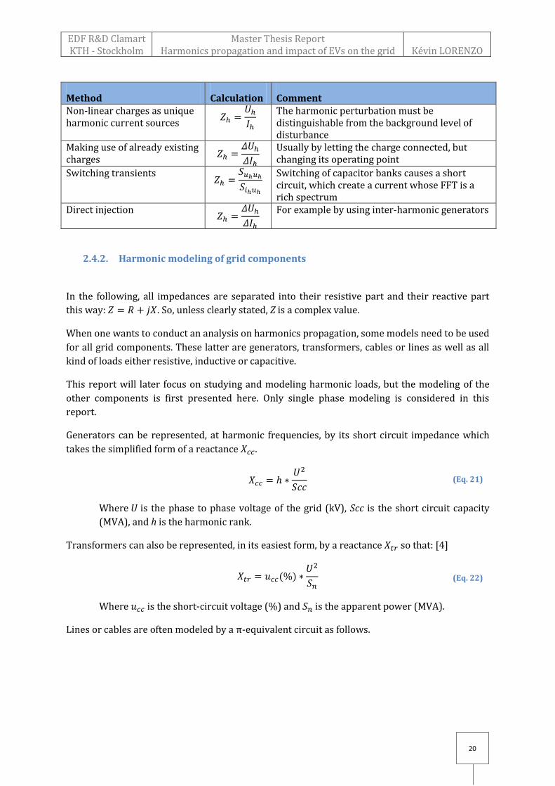
2.4.2. Harmonic modeling of grid components
In the following, all impedances are separated into their resistive part and their reactive part
this way: . So, unless clearly stated, Z is a complex value.
When one wants to conduct an analysis on harmonics propagation, some models need to be used
for all grid components. These latter are generators, transformers, cables or lines as well as all
kind of loads either resistive, inductive or capacitive.
This report will later focus on studying and modeling harmonic loads, but the modeling of the
other components is first presented here. Only single phase modeling is considered in this
report.
Generators can be represented, at harmonic frequencies, by its short circuit impedance which
takes the simplified form of a reactance .
Where is the phase to phase voltage of the grid (kV), Scc is the short circuit capacity
(MVA), and h is the harmonic rank.
Transformers can also be represented, in its easiest form, by a reactance so that: [4]
( )
Where is the short-circuit voltage (%) and is the apparent power (MVA).
Lines or cables are often modeled by a -equivalent circuit as follows.
EDF R&D Clamart KTH - Stockholm
Master Thesis Report Harmonics propagation and impact of EVs on the grid
Kévin LORENZO
21
(Eq. 23)
Figure 8: Pi-Equivalent model of lines/cables
Where the resistance is obtained with the resistivity , the cable length L and the cable
section S so that
. The reactance can be approximated [4] to be and
the capacity, which is especially important for coaxial cables, is calculated [12] with
( ) where K is the dielectric constant and and are inner and
outer conductor radiuses.
Capacitor banks are simply represented by a negative reactance and added to the grid as
shunt capacitors:
Several ways [13] can be found in the literature to model a load, or an aggregation of loads. Some
of these models only come from a separation between active and reactive power, some from
experimental results of measurement campaigns, or from assumptions on the load structure.
The main parameters of these models are the voltage level, the active and reactive power that it
absorbs and the harmonic rank. Six of them are presented below, by their equivalent 1-phase
circuit.
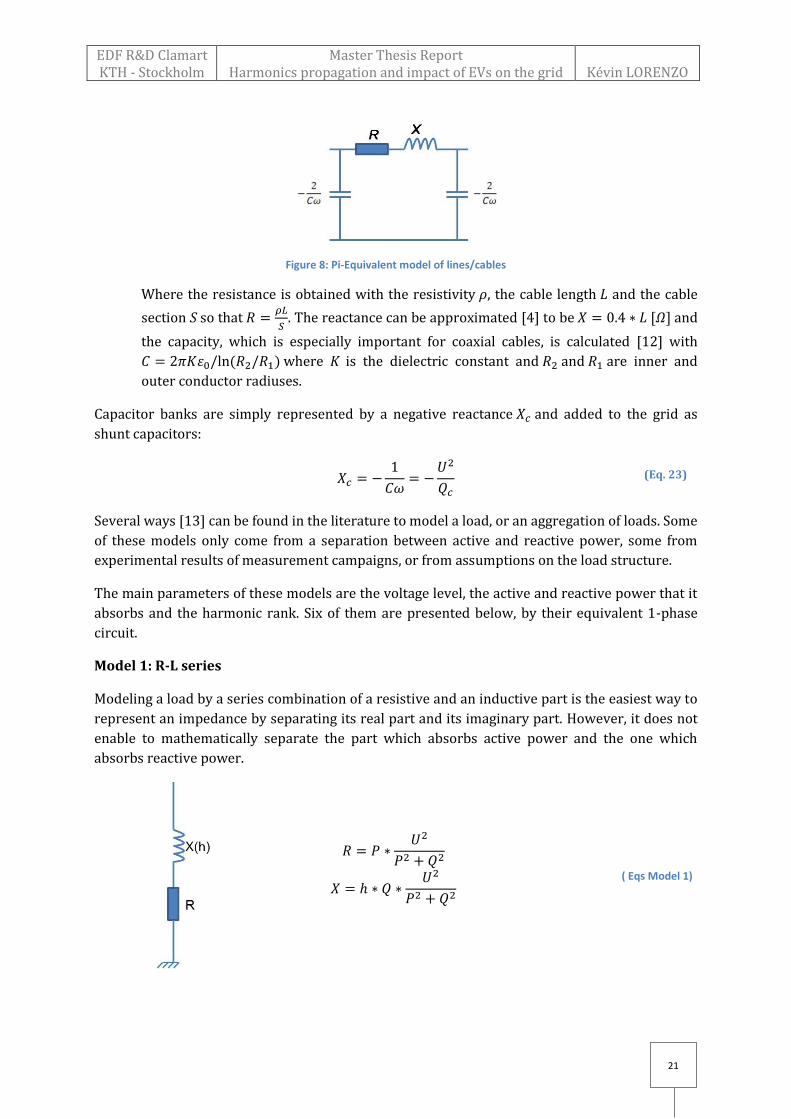
Model 1: R-L series
Modeling a load by a series combination of a resistive and an inductive part is the easiest way to
represent an impedance by separating its real part and its imaginary part. However, it does not
enable to mathematically separate the part which absorbs active power and the one which
absorbs reactive power.
( Eqs Model 1)

EDF R&D Clamart KTH - Stockholm
Master Thesis Report Harmonics propagation and impact of EVs on the grid
Kévin LORENZO
22
is the phase to phase voltage of the grid, P and Q are the active and reactive power absorbed
by the charge, and h is the harmonic rank.
Model 2 : R//L parallel
A parallel combination of a resistive and an inductive part is an easy way to model a load by
separating the part of the load which absorbs active power and the one which absorbs reactive
power.
( Eqs Model 2)
Model 3 : R//L parallel + skin effect
Taking into account the skin effect in the previous model, the following one is obtained.
( )
( )
( )
( Eqs Model 3)
( ) represents the skin effect [14] [13]. This model was suggested several times
in the literature under this form, and for this reason was presented and studied here. However,
the modeling of skin effect is doubted. Indeed, with these equations, it seems that the higher the
frequency, the lower the resistance. This is unintuitive since at high frequencies, the skin depth
is reduced, meaning that the conductors section where the current mostly flows is reduced. With
a reduced section, the resistance should be higher.
Model 4 : Induction motor
This model takes into account the fraction K of motive load in the total load demand, which
means the part of active power absorbed by induction motors on the whole active power
absorbed. It is generally used when K has a relatively high value (when the load is
predominantly motive [13]).

EDF R&D Clamart KTH - Stockholm
Master Thesis Report Harmonics propagation and impact of EVs on the grid
Kévin LORENZO
23
( )
( Eqs Model 4)
is the reactance with blocked rotors in p.u. (usually from 0.15 to 0.25 p.u. [15]), K is the
fraction of motive load in the total load demand, is the install factor (usually around 1.2).
represents the resistive part of the load while represents the motive one.
Model 5 : CIGRE model
This model is the one recommended by CIGRE (International council on large electric systems).
The formulas below come from experimental data obtained on MV systems [16]. As a harmonic
model, it is said to be valid for harmonic ranks from 5 to 20.
( )
( Eqs Model 5)
( ) is the ratio .
Model 6 : (R-L)//(R-L)
If the charge consists of a large part of motors, the model 4 can be made more complex by adding
a resistive part to the motive one and vice versa.
( )
( Eqs Model 6)
EDF R&D Clamart KTH - Stockholm
Master Thesis Report Harmonics propagation and impact of EVs on the grid
Kévin LORENZO
24
is the quality factor . [13]
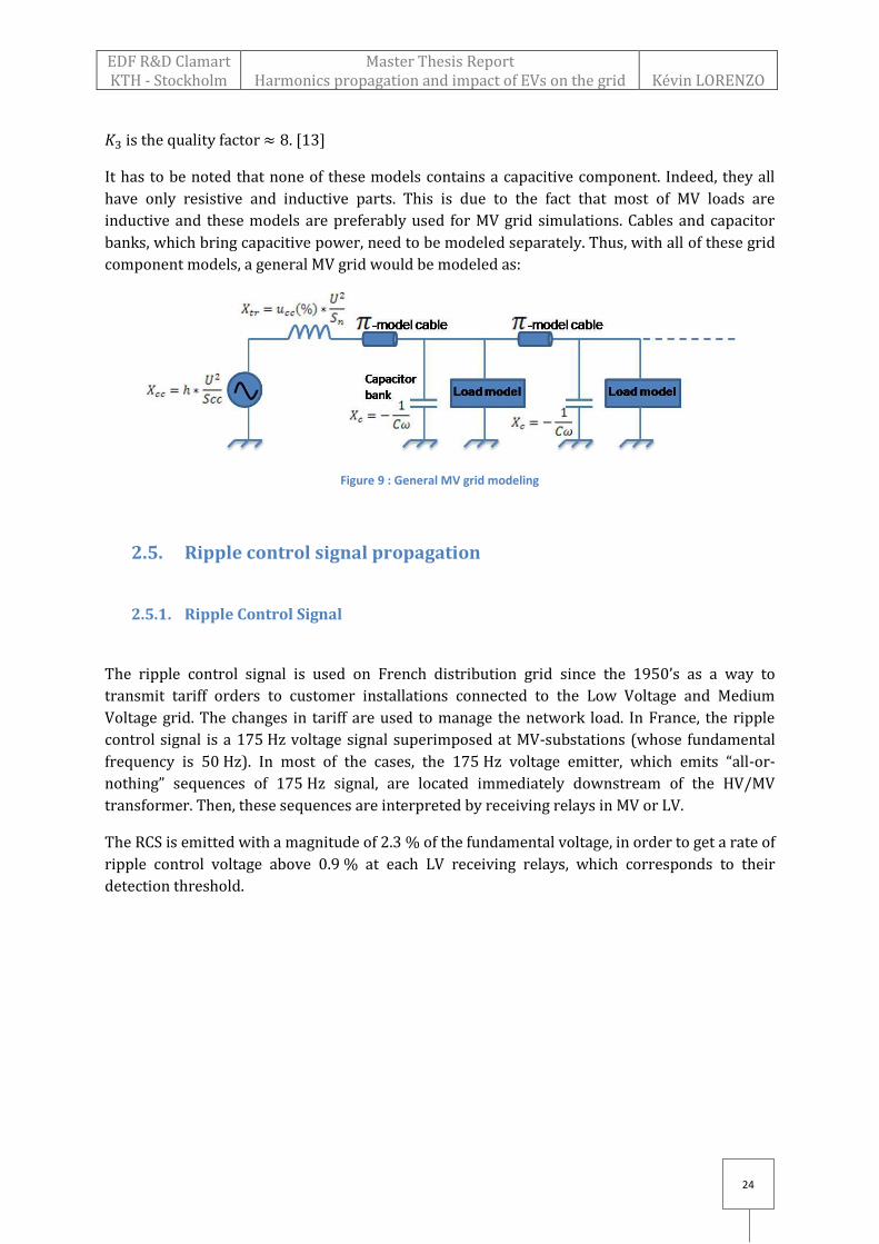
It has to be noted that none of these models contains a capacitive component. Indeed, they all
have only resistive and inductive parts. This is due to the fact that most of MV loads are
inductive and these models are preferably used for MV grid simulations. Cables and capacitor
banks, which bring capacitive power, need to be modeled separately. Thus, with all of these grid
component models, a general MV grid would be modeled as:
Figure 9 : General MV grid modeling
2.5. Ripple control signal propagation
2.5.1. Ripple Control Signal
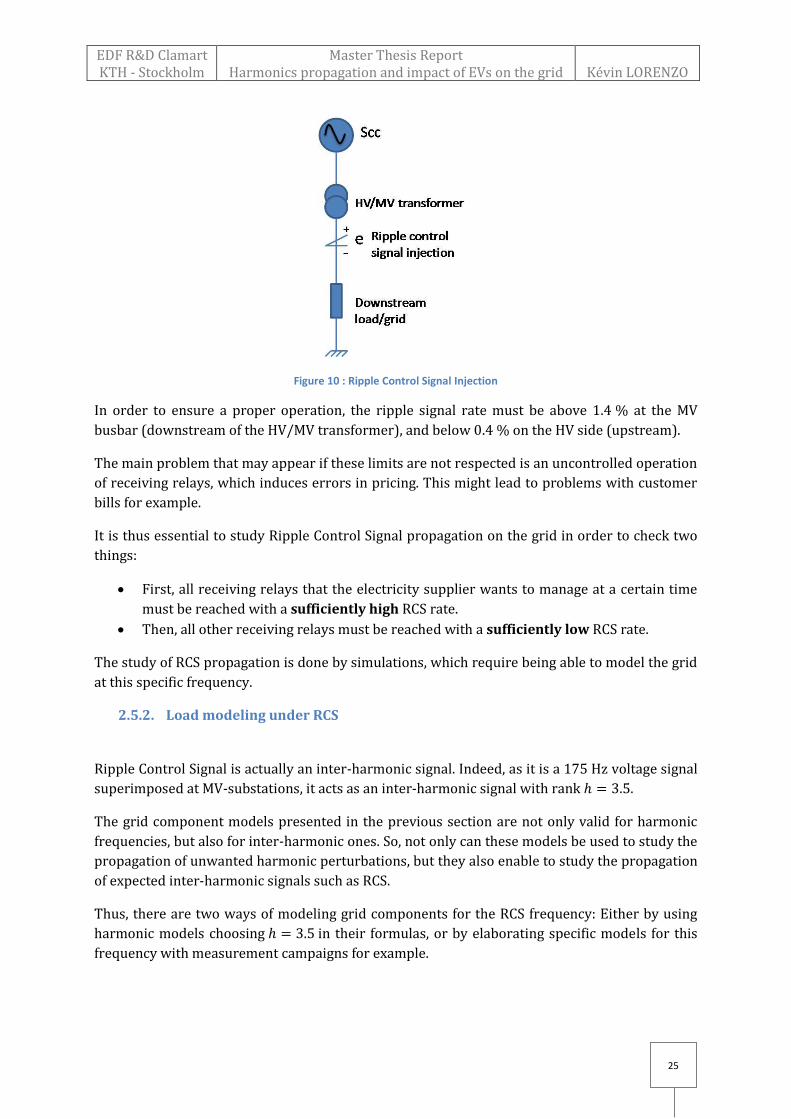
The ripple control signal is used on French distribution grid since the 1950’s as a way to
transmit tariff orders to customer installations connected to the Low Voltage and Medium
Voltage grid. The changes in tariff are used to manage the network load. In France, the ripple
control signal is a 175 Hz voltage signal superimposed at MV-substations (whose fundamental
frequency is 50 Hz). In most of the cases, the 175 Hz voltage emitter, which emits “all-or-
nothing” sequences of 175 Hz signal, are located immediately downstream of the HV/MV
transformer. Then, these sequences are interpreted by receiving relays in MV or LV.
The RCS is emitted with a magnitude of 2.3 % of the fundamental voltage, in order to get a rate of
ripple control voltage above 0.9 % at each LV receiving relays, which corresponds to their
detection threshold.
EDF R&D Clamart KTH - Stockholm
Master Thesis Report Harmonics propagation and impact of EVs on the grid
Kévin LORENZO
25
Figure 10 : Ripple Control Signal Injection
In order to ensure a proper operation, the ripple signal rate must be above 1.4 % at the MV
busbar (downstream of the HV/MV transformer), and below 0.4 % on the HV side (upstream).
The main problem that may appear if these limits are not respected is an uncontrolled operation
of receiving relays, which induces errors in pricing. This might lead to problems with customer
bills for example.
It is thus essential to study Ripple Control Signal propagation on the grid in order to check two
things:
First, all receiving relays that the electricity supplier wants to manage at a certain time
must be reached with a sufficiently high RCS rate.
Then, all other receiving relays must be reached with a sufficiently low RCS rate.
The study of RCS propagation is done by simulations, which require being able to model the grid
at this specific frequency.
2.5.2. Load modeling under RCS
Ripple Control Signal is actually an inter-harmonic signal. Indeed, as it is a 175 Hz voltage signal
superimposed at MV-substations, it acts as an inter-harmonic signal with rank .
The grid component models presented in the previous section are not only valid for harmonic
frequencies, but also for inter-harmonic ones. So, not only can these models be used to study the
propagation of unwanted harmonic perturbations, but they also enable to study the propagation
of expected inter-harmonic signals such as RCS.
Thus, there are two ways of modeling grid components for the RCS frequency: Either by using
harmonic models choosing in their formulas, or by elaborating specific models for this
frequency with measurement campaigns for example.

EDF R&D Clamart KTH - Stockholm
Master Thesis Report Harmonics propagation and impact of EVs on the grid
Kévin LORENZO
26
III. Study of EVs harmonic behavior and modeling
This section presents a study that was done within the context of this internship. It concerns the
characterization of the harmonic currents emitted by different vehicles that were tested in
laboratory. First, several vehicle models were tested separately, and then measurements were
carried out on several cars of the same model simultaneously. From the unit tests, a model for
each car was drawn, which enables to perform simulations on an existing car park. These
simulations as well as measurements are presented in the “Case study 1”.
3.1. Unit testing on existing cars Unit testing of EVs in a laboratory are a way to apprehend their harmonic behavior. Indeed, it
enables to study the car charging under controlled conditions, and to implement a process which
makes the studies independent from the point of the grid where it is studied. Therefore, it has
been chosen during this project to first perform these experiments on individual cars in
laboratory, then on several cars at the same time and then to draw a harmonic model from them
for each kind of car tested.
3.1.1. Unit testing process
The process presented here has been performed on several car models, directly in the
laboratory of the Power Quality group at EDF R&D.
For each EV model, the aim was to perform a complete charging cycle while measuring the
current absorbed by the vehicle, and the voltage across. The charging mode 3 was used, which
means that the car is connected to the Low Voltage grid (230 V) through a single phase charging
station which communicates with the car during the charging [9]. The charging station used
during the experiments has a 3 kW nominal power.
In order to study the impact of the EV only on power quality, and in reference conditions, a
power amplifier has been connected between the grid and the charging station during the
testing. This power amplifier has been set to provide a perfectly sinusoidal voltage throughout
the tests. Thereby, the study has been made independent of the point of the grid where the
amplifier is connected.
The laboratory layout is presented below.

EDF R&D Clamart KTH - Stockholm
Master Thesis Report Harmonics propagation and impact of EVs on the grid
Kévin LORENZO
27
Figure 11 : Unit testing layout
The measurements have been performed using a prototype developed within the Power Quality
group (see picture below). With this prototype, the harmonic current and voltage values are
obtained in the frequency range 0 to 2 kHz, with a 100 kHz sampling frequency.
Figure 12 : Data acquisition system
The currents measurements have been performed with two Hall Effect current probes, in order
to get both the phase current and the neutral current.
3.1.2. Results of measurements: Harmonic behavior of EVs
Four different car models have been tested in the laboratory. Two of these vehicles are
presented in this report, and are called EV1 and EV2, due to confidentiality reasons.

EDF R&D Clamart KTH - Stockholm
Master Thesis Report Harmonics propagation and impact of EVs on the grid
Kévin LORENZO
28
The characteristics of these vehicles, as well as the ones for the vehicle EV3 which will be
studied in the “Case study” part, are summed up below.
Table 3: Electric vehicles caracteristics
Vehicle model Battery type Battery capacity
Charging current
Charging mode tested
EV1 Lithium-ion 22 kWh 16 A Mode 3 EV2 Lithium-ion 22 kWh 16 A Mode 3 EV3 Lithium-ion 16 kWh 9 A Mode 3
The complete charging cycle lasts between 5h and 8h, depending on the battery size and the
level of current absorbed. This cycle usually contains three different phases: the charging start
where the current absorbed by the EV increases quickly, the main charging phase where the
current remains quasi-constant, and the end of charging where the current absorbed slowly
decreases. The figure below shows an example of a complete charging cycle.
Figure 13 : Example of an electric vehicle (EV1) charging cycle
Due to the presence of the power amplifier, the voltage waveform is very close to a perfect sine
wave. However, a harmonic distortion is clearly visible on the current waveform. The figure
below shows these waveforms for one of the vehicles tested.
15,75 A
0
5
10
15
20
11
73
34
96
58
19
71
13
12
91
45
16
11
77
19
32
09
22
52
41
25
72
73
28
93
05
32
13
37
35
33
69
38
54
01
I (A
)
t (min)
RMS Current evolution throughout the charging cycle

EDF R&D Clamart KTH - Stockholm
Master Thesis Report Harmonics propagation and impact of EVs on the grid
Kévin LORENZO
29
Figure 14 : EV1 current waveform during the “main charging” phase
For this vehicle operating in the main charging phase, small peaks and small dips can
alternatively be noticed close to the current zero crossing. During the end of charging phase, the
current waveform is even more distorted compared to an ideal sinusoid. It can be noticed that,
the lower the fundamental current is during this phase, the more the waveform seems distorted.
However, this doesn’t mean that the harmonic currents are higher in magnitude during this
phase, but their contributions in percentage to RMS current are higher.
Figure 15 : EV1 current waveform during the “end of charging” phase
As it can be seen on the two figures above, EVs don’t absorb sinusoidal currents during their
charging cycle. Therefore, they emit harmonic currents which spread on the grid, and create
harmonic voltages.
All the vehicles used to make unit testing absorb a current below 16 A, thus they are subject to
the standard IEC 61000-3-2. However, the harmonic current values measured during the
laboratory experiments cannot be directly compared to the standard level. Indeed, as explained
in the “harmonic measurements” part, some specific conditions, such as harmonic grouping or
smoothing filtering, need to be applied to make a direct comparison. The prototype used in the
laboratory to make the measurement doesn’t strictly comply with these conditions. This can be
explained by the fact that the aim when proceeding to such laboratory measurements is to
EDF R&D Clamart KTH - Stockholm
Master Thesis Report Harmonics propagation and impact of EVs on the grid
Kévin LORENZO
30
investigate the phenomena that may appear for some harmonic frequencies. Thus, as they are
not used to check the compliance to standards, the measurements don’t need to be carried out in
the exact same conditions than the ones described in IEC 61000-3-2. However, in order to have
an idea of the harmonic levels measured, the results can be compared to the standard for
informational purposes. The same reasoning also applies to the voltage harmonics, in regards to
the EN50160 standard.
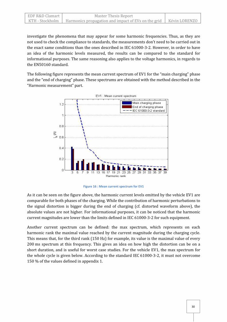
The following figure represents the mean current spectrum of EV1 for the “main charging” phase
and the “end of charging” phase. These spectrums are obtained with the method described in the
“Harmonic measurement” part.
Figure 16 : Mean current spectrum for EV1
As it can be seen on the figure above, the harmonic current levels emitted by the vehicle EV1 are
comparable for both phases of the charging. While the contribution of harmonic perturbations to
the signal distortion is bigger during the end of charging (cf. distorted waveform above), the
absolute values are not higher. For informational purposes, it can be noticed that the harmonic
current magnitudes are lower than the limits defined in IEC 61000-3-2 for such equipment.
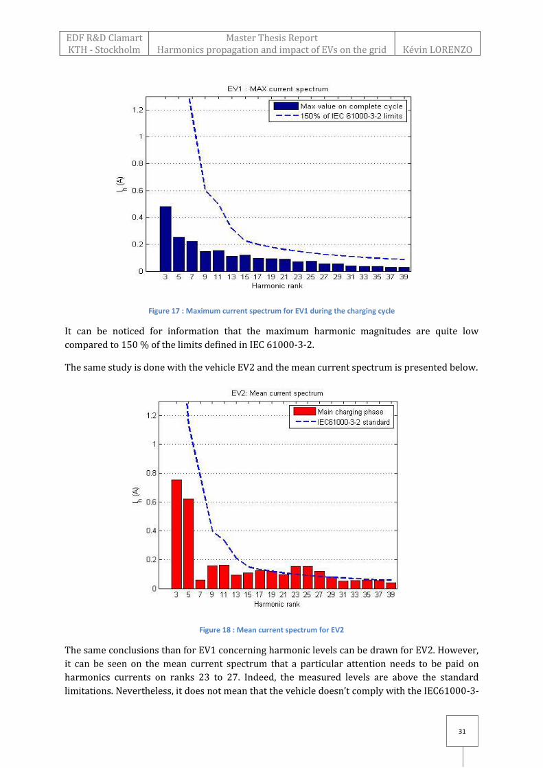
Another current spectrum can be defined: the max spectrum, which represents on each
harmonic rank the maximal value reached by the current magnitude during the charging cycle.
This means that, for the third rank (150 Hz) for example, its value is the maximal value of every
200 ms spectrum at this frequency. This gives an idea on how high the distortion can be on a
short duration, and is useful for worst case studies. For the vehicle EV1, the max spectrum for
the whole cycle is given below. According to the standard IEC 61000-3-2, it must not overcome
150 % of the values defined in appendix 1.
EDF R&D Clamart KTH - Stockholm
Master Thesis Report Harmonics propagation and impact of EVs on the grid
Kévin LORENZO
31
Figure 17 : Maximum current spectrum for EV1 during the charging cycle
It can be noticed for information that the maximum harmonic magnitudes are quite low
compared to 150 % of the limits defined in IEC 61000-3-2.
The same study is done with the vehicle EV2 and the mean current spectrum is presented below.
Figure 18 : Mean current spectrum for EV2
The same conclusions than for EV1 concerning harmonic levels can be drawn for EV2. However,
it can be seen on the mean current spectrum that a particular attention needs to be paid on
harmonics currents on ranks 23 to 27. Indeed, the measured levels are above the standard
limitations. Nevertheless, it does not mean that the vehicle doesn’t comply with the IEC61000-3-

EDF R&D Clamart KTH - Stockholm
Master Thesis Report Harmonics propagation and impact of EVs on the grid
Kévin LORENZO
32
2 standard, because as explained above, the measurements were not performed in standard
conditions. Thus, a direct comparison is not possible. But except for the 7th rank, harmonic
currents are slightly higher for EV2 than for EV1.
During the charging cycle, the harmonic distortion does not vary much. The temporal evolution
of which gives information on the whole harmonic content, is plotted below for the
charging cycle of the vehicle EV1 and EV2.
Figure 19 : Temporal evolution of the current harmonic distortion during the charging cycle
The current THD is higher for EV2 than for EV1 during its charging cycle. However, it remains
quite low (between 5% and 7%).
What can also be noticed is that the harmonic distortion is almost constant during the “main
charging” phase for EV1, which means that every 2min30s period can be chosen as
representative of this behavior to compute the mean spectrum. For EV2 though, as harmonic
distortions are higher during the second part of the charging cycle, the mean spectrum needs to
be calculated during this period.
3.1.3. EV behavior at higher frequencies
During laboratory measurements, a particular behavior of Electric Vehicles was observed at
higher frequencies than the harmonic range [0 – 2 kHz]. In order to study those kinds of
perturbations, another prototype has been used during laboratory measurements. This second
prototype enables to study frequential distortions in the range [2 kHz – 150 kHz], with a 1 MHz
sampling frequency. It was placed at the exact same place than the first one.
As the first prototype described before, this second one gives a voltage spectrum and a current
spectrum every 200 ms. However, this spectrum is obtained in the range [2 kHz – 150 kHz] with
a 200 Hz step. Thus, the grouping of every 5 Hz contribution is done this way:
0
1
2
3
4
5
6
7
8
9
1
22
43
64
85
10
6
12
7
14
8
16
9
19
0
21
1
23
2
25
3
27
4
29
5
31
6
33
7
35
8
37
9
40
0
42
1
44
2
46
3
%
t (min)
Current distortion comparison
THDi% for EV1
THDi% for EV2
EDF R&D Clamart KTH - Stockholm
Master Thesis Report Harmonics propagation and impact of EVs on the grid
Kévin LORENZO
33
(Eq. 24,25)
√
√
…
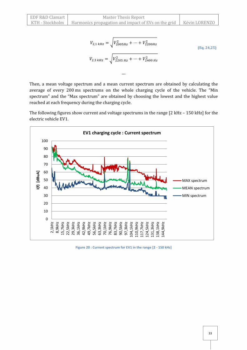
Then, a mean voltage spectrum and a mean current spectrum are obtained by calculating the
average of every 200 ms spectrums on the whole charging cycle of the vehicle. The “Min
spectrum” and the “Max spectrum” are obtained by choosing the lowest and the highest value
reached at each frequency during the charging cycle.
The following figures show current and voltage spectrums in the range [2 kHz – 150 kHz] for the
electric vehicle EV1.
Figure 20 : Current spectrum for EV1 in the range [2 - 150 kHz]
0
10
20
30
40
50
60
70
80
90
100
2,1
kHz
8,9
kHz
15
,7kH
z
22
,5kH
z
29
,3kH
z
36
,1kH
z
42
,9kH
z
49
,7kH
z
56
,5kH
z
63
,3kH
z
70
,1kH
z
76
,9kH
z
83
,7kH
z
90
,5kH
z
97
,3kH
z
10
4,1
kHz
11
0,9
kHz
11
7,7
kHz
12
4,5
kHz
13
1,3
kHz
13
8,1
kHz
14
4,9
kHz
I(f)
[d
Bu
A]
EV1 charging cycle : Current spectrum
MAX spectrum
MEAN spectrum
MIN spectrum

EDF R&D Clamart KTH - Stockholm
Master Thesis Report Harmonics propagation and impact of EVs on the grid
Kévin LORENZO
34
Figure 21 : Voltage spectrum for EV1 in the range [2 - 150 kHz]
NB: The spectrums of this section are expressed in dBµA (or in dBµV). For information,
120 dBµA represent 1 A and 120 dBµV represent 1 V.
During EV1 charging cycle, the perturbations in this range of frequencies have mean values
around 80 dBµV and 90 dBµA close to 2 kHz, which in general decrease until 60 dBµV and
40 dBµA around 150 kHz. What can be observed with these spectrums is the apparition of peaks
at certain frequencies. For example, at 6.7 kHz, there is a perturbation peak both in current and
in voltage, which probably corresponds to the PWM frequency of the Battery Management
System.
There is also a peak on the current spectrum around 70 kHz, that doesn’t really appear on the
voltage spectrum, and whose origin is unknown. The big peak around 100 kHz both in current
and in voltage correspond to the power amplifier switching frequency.
However, the values observed on these spectrums cannot be compared to any standards in this
range of frequency. Indeed, there is no limit today for voltages emission or absorption in the
frequency range [2-150 kHz] concerning electric vehicles. It is thus relatively difficult to analyze
the levels observed above and to assess if they might cause problems to the grid. However, one
cannot assure that sensitive equipment connected to the grid will not be affected [17].
3.2. Multiple testing on 4 EVs
Within the context of the study on Electric Vehicles harmonic behavior, some measurements
were also performed on 4 vehicles of type “EV1” simultaneously. The analysis of these
0
20
40
60
80
100
1202
,1kH
z
8,9
kHz
15
,7kH
z
22
,5kH
z
29
,3kH
z
36
,1kH
z
42
,9kH
z
49
,7kH
z
56
,5kH
z
63
,3kH
z
70
,1kH
z
76
,9kH
z
83
,7kH
z
90
,5kH
z
97
,3kH
z
10
4,1
kHz
11
0,9
kHz
11
7,7
kHz
12
4,5
kHz
13
1,3
kHz
13
8,1
kHz
14
4,9
kHz
V(f
) [
dB
uV
]
EV1 charging cycle : Voltage spectrum
MAX spectrum
MEAN spectrum
MIN spectrum
EDF R&D Clamart KTH - Stockholm
Master Thesis Report Harmonics propagation and impact of EVs on the grid
Kévin LORENZO
35
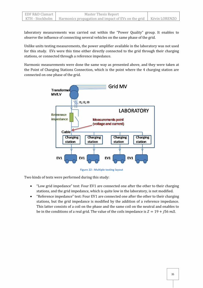
laboratory measurements was carried out within the “Power Quality” group. It enables to
observe the influence of connecting several vehicles on the same phase of the grid.
Unlike units testing measurements, the power amplifier available in the laboratory was not used
for this study. EVs were this time either directly connected to the grid through their charging
stations, or connected through a reference impedance.
Harmonic measurements were done the same way as presented above, and they were taken at
the Point of Charging Stations Connection, which is the point where the 4 charging station are
connected on one phase of the grid.
Figure 22 : Multiple testing layout
Two kinds of tests were performed during this study:
“Low grid impedance” test: Four EV1 are connected one after the other to their charging
stations, and the grid impedance, which is quite low in the laboratory, is not modified.
“Reference impedance” test: Four EV1 are connected one after the other to their charging
stations, but the grid impedance is modified by the addition of a reference impedance.
This latter consists of a coil on the phase and the same coil on the neutral and enables to
be in the conditions of a real grid. The value of the coils impedance is .
EDF R&D Clamart KTH - Stockholm
Master Thesis Report Harmonics propagation and impact of EVs on the grid
Kévin LORENZO
36
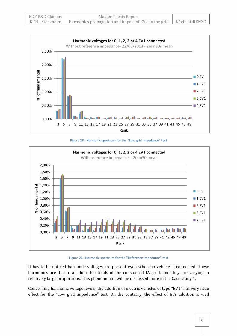
Figure 23 : Harmonic spectrum for the "Low grid impedance" test
Figure 24 : Harmonic spectrum for the "Reference impedance" test
It has to be noticed harmonic voltages are present even when no vehicle is connected. These
harmonics are due to all the other loads of the considered LV grid, and they are varying in
relatively large proportions. This phenomenon will be discussed more in the Case study 1.
Concerning harmonic voltage levels, the addition of electric vehicles of type “EV1” has very little
effect for the “Low grid impedance” test. On the contrary, the effect of EVs addition is well
0,00%
0,50%
1,00%
1,50%
2,00%
2,50%
3 5 7 9 11 13 15 17 19 21 23 25 27 29 31 33 35 37 39 41 43 45 47 49
% o
f fu
nd
ame
nta
l
Rank
Harmonic voltages for 0, 1, 2, 3 or 4 EV1 connected Without reference impedance- 22/05/2013 - 2min30s mean
0 EV
1 EV1
2 EV1
3 EV1
4 EV1
0,00%
0,20%
0,40%
0,60%
0,80%
1,00%
1,20%
1,40%
1,60%
1,80%
2,00%
3 5 7 9 11 13 15 17 19 21 23 25 27 29 31 33 35 37 39 41 43 45 47 49
% o
f fu
nd
ame
nta
l
Rank
Harmonic voltages for 0, 1, 2, 3 or 4 EV1 connected With reference impedance - 2min30 mean
0 EV
1 EV1
2 EV1
3 EV1
4 EV1
EDF R&D Clamart KTH - Stockholm
Master Thesis Report Harmonics propagation and impact of EVs on the grid
Kévin LORENZO
37
observable for the “Reference impedance” test. Indeed, for this latter, the perturbations are
clearly increased when new vehicles are connected.
Thus, the impact of EVs on the power quality actually strongly depends on the upstream
impedance at the point of connection. The lower it is, the lower are the harmonic voltages
caused by EVs.
The electric car park that will be studied in Case study 1 contains 10 charging stations. These
stations are distributed on the three phases of the LV grid. This means that at most 4 EVs can be
connected to one of its phases. This is the reason why this multiple testing on 4 EV1 were
conducted.
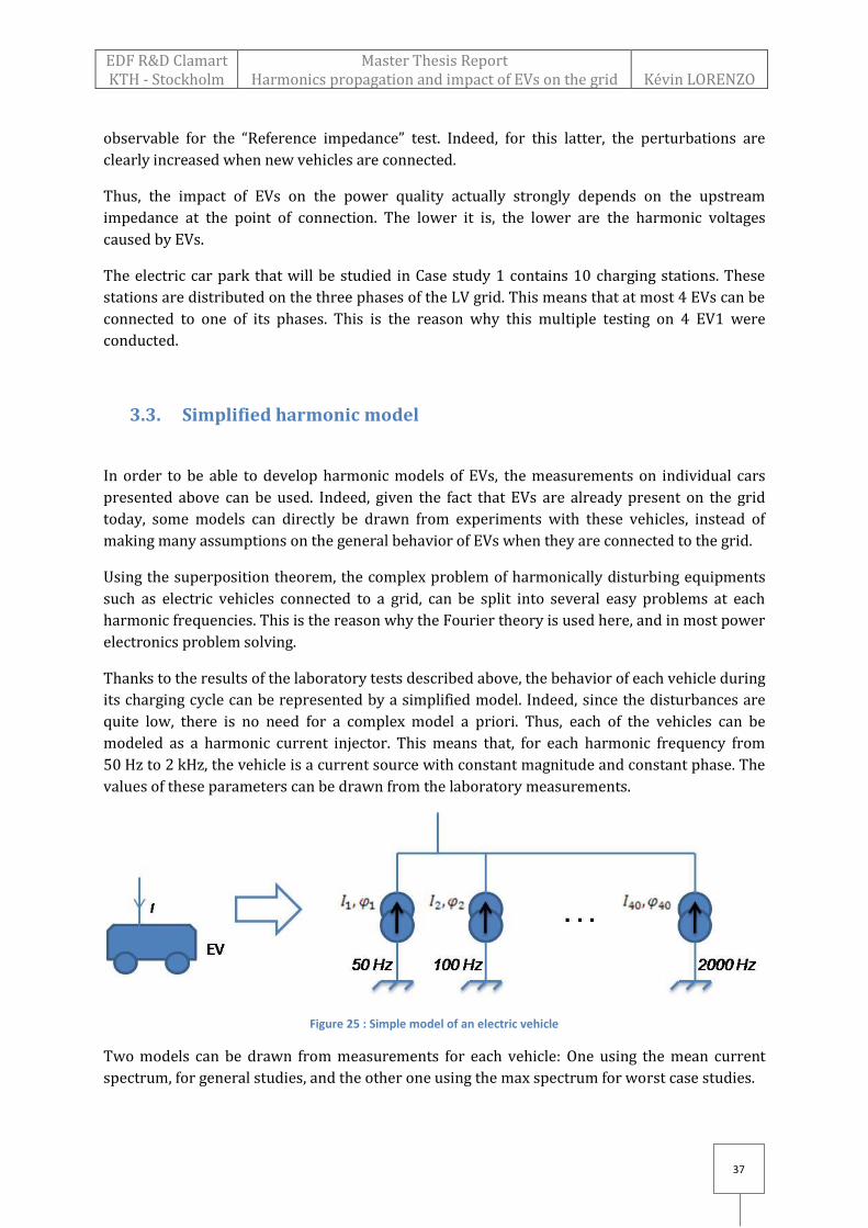
3.3. Simplified harmonic model
In order to be able to develop harmonic models of EVs, the measurements on individual cars
presented above can be used. Indeed, given the fact that EVs are already present on the grid
today, some models can directly be drawn from experiments with these vehicles, instead of
making many assumptions on the general behavior of EVs when they are connected to the grid.
Using the superposition theorem, the complex problem of harmonically disturbing equipments
such as electric vehicles connected to a grid, can be split into several easy problems at each
harmonic frequencies. This is the reason why the Fourier theory is used here, and in most power
electronics problem solving.
Thanks to the results of the laboratory tests described above, the behavior of each vehicle during
its charging cycle can be represented by a simplified model. Indeed, since the disturbances are
quite low, there is no need for a complex model a priori. Thus, each of the vehicles can be
modeled as a harmonic current injector. This means that, for each harmonic frequency from
50 Hz to 2 kHz, the vehicle is a current source with constant magnitude and constant phase. The
values of these parameters can be drawn from the laboratory measurements.
Figure 25 : Simple model of an electric vehicle
Two models can be drawn from measurements for each vehicle: One using the mean current
spectrum, for general studies, and the other one using the max spectrum for worst case studies.

EDF R&D Clamart KTH - Stockholm
Master Thesis Report Harmonics propagation and impact of EVs on the grid
Kévin LORENZO
38
The software that is used for simulations is called Expertec. It allows to perform analyzes of
electrical circuit in the frequency domain, combining both the calculations for the fundamental
frequency (50 Hz) and for the harmonic frequencies. In this software one can define a multi-
frequential current source, by setting for each harmonic frequency a magnitude and a phase.
Thus, in order to obtain the model of the vehicle EV1, one needs to set a magnitude and a phase
on each harmonic rank from 1 to 40. Concerning the magnitude, the values are simply obtained
with the mean current spectrum from measurements presented above. Concerning the phase,
the values are also obtained from the measurements. Indeed, the prototype used in the
laboratory records the phase of voltage and current. As the phases are all almost constant during
the charging cycle of the vehicle, there is no need to calculate an average on the complete cycle.
A shorter period is representative of the phase behavior.
For EV1, the current magnitude spectrum is given above, and the current phase spectrum is
represented below.
Figure 26 : Current phase spectrum of EV1
With these magnitudes and these phases for the current absorbed by EV1, the following current
wave is obtained by an inverse Fourier transform.
Figure 27 : Inverse Fourier transform of EV1's model
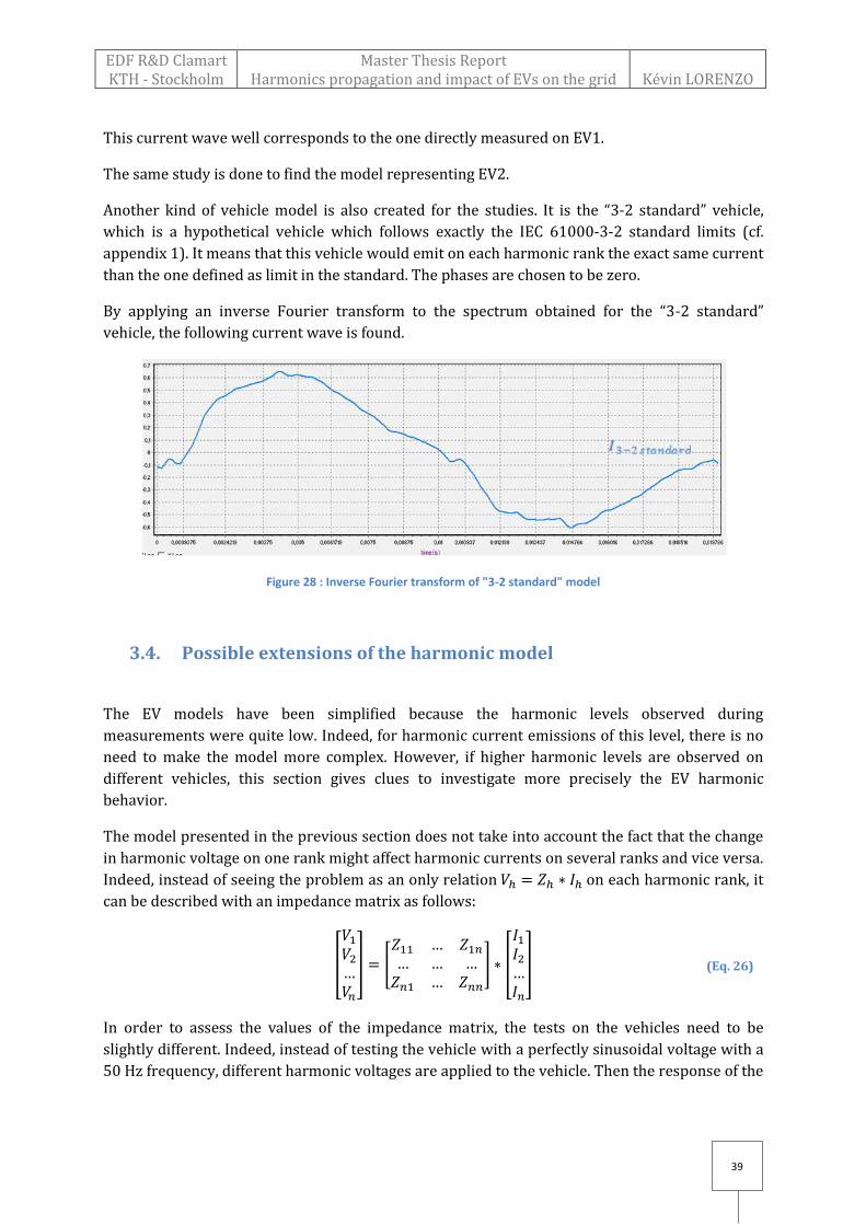
EDF R&D Clamart KTH - Stockholm
Master Thesis Report Harmonics propagation and impact of EVs on the grid
Kévin LORENZO
39
(Eq. 26)
This current wave well corresponds to the one directly measured on EV1.
The same study is done to find the model representing EV2.
Another kind of vehicle model is also created for the studies. It is the “3-2 standard” vehicle,
which is a hypothetical vehicle which follows exactly the IEC 61000-3-2 standard limits (cf.
appendix 1). It means that this vehicle would emit on each harmonic rank the exact same current
than the one defined as limit in the standard. The phases are chosen to be zero.
By applying an inverse Fourier transform to the spectrum obtained for the “3-2 standard”
vehicle, the following current wave is found.
Figure 28 : Inverse Fourier transform of "3-2 standard" model
3.4. Possible extensions of the harmonic model
The EV models have been simplified because the harmonic levels observed during
measurements were quite low. Indeed, for harmonic current emissions of this level, there is no
need to make the model more complex. However, if higher harmonic levels are observed on
different vehicles, this section gives clues to investigate more precisely the EV harmonic
behavior.
The model presented in the previous section does not take into account the fact that the change
in harmonic voltage on one rank might affect harmonic currents on several ranks and vice versa.
Indeed, instead of seeing the problem as an only relation on each harmonic rank, it
can be described with an impedance matrix as follows:
[
] [
] [
]
In order to assess the values of the impedance matrix, the tests on the vehicles need to be
slightly different. Indeed, instead of testing the vehicle with a perfectly sinusoidal voltage with a
50 Hz frequency, different harmonic voltages are applied to the vehicle. Then the response of the

EDF R&D Clamart KTH - Stockholm
Master Thesis Report Harmonics propagation and impact of EVs on the grid
Kévin LORENZO
40
vehicle in terms of harmonic currents is observed and the impedance matrix is filled step by
step.
This modeling enables to add to the study the fact that several vehicles connected to the same
phase on a grid can perturb each other. Indeed, let’s assume that a feeding grid is perfectly
sinusoidal. When a vehicle is connected to one of its phases, the voltage is distorted by the
vehicle harmonic currents. Thus, if a second vehicle is connected to this phase, the voltage that it
sees is already distorted by the first vehicle, and its behavior may be changed. The problem as it
is described in the previous section cannot represent this influence of one vehicle on another.
But with an impedance matrix, it can be modeled.
This other way of modeling would give more precise results. But, it needs more measures and
investigations to be done. Also, such a study would require post-treatment tools that are
currently being developed in the Power Quality group. Thus, this solution was not chosen in the
context of this thesis. However, this section gives tudy perspectives for future models..
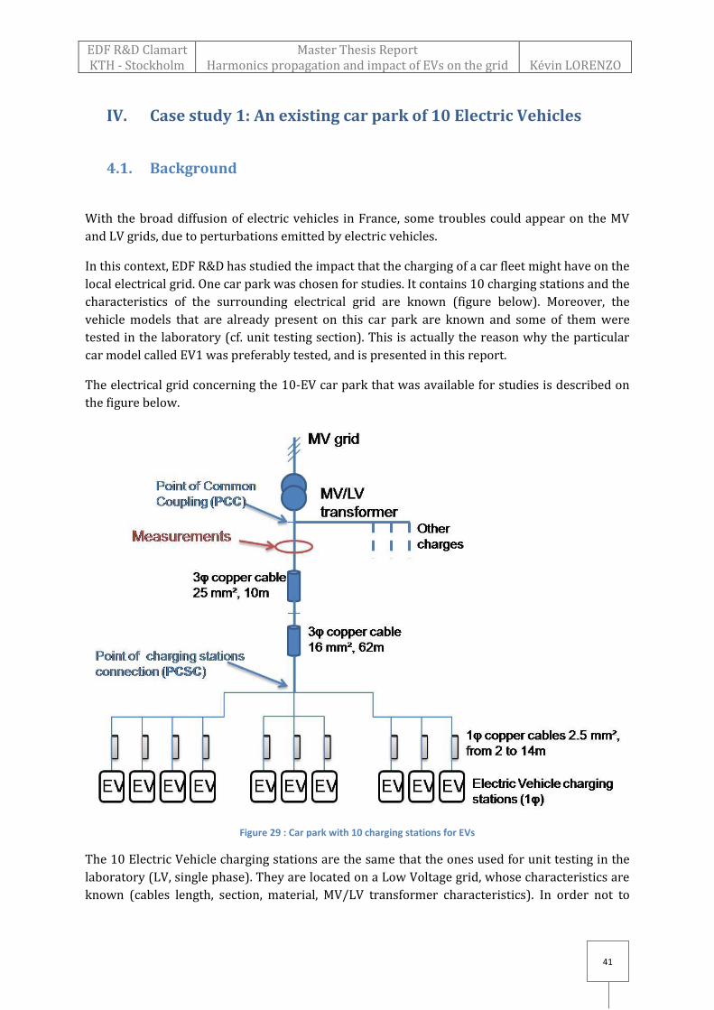
EDF R&D Clamart KTH - Stockholm
Master Thesis Report Harmonics propagation and impact of EVs on the grid
Kévin LORENZO
41
IV. Case study 1: An existing car park of 10 Electric Vehicles
4.1. Background
With the broad diffusion of electric vehicles in France, some troubles could appear on the MV
and LV grids, due to perturbations emitted by electric vehicles.
In this context, EDF R&D has studied the impact that the charging of a car fleet might have on the
local electrical grid. One car park was chosen for studies. It contains 10 charging stations and the
characteristics of the surrounding electrical grid are known (figure below). Moreover, the
vehicle models that are already present on this car park are known and some of them were
tested in the laboratory (cf. unit testing section). This is actually the reason why the particular
car model called EV1 was preferably tested, and is presented in this report.
The electrical grid concerning the 10-EV car park that was available for studies is described on
the figure below.
Figure 29 : Car park with 10 charging stations for EVs
The 10 Electric Vehicle charging stations are the same that the ones used for unit testing in the
laboratory (LV, single phase). They are located on a Low Voltage grid, whose characteristics are
known (cables length, section, material, MV/LV transformer characteristics). In order not to
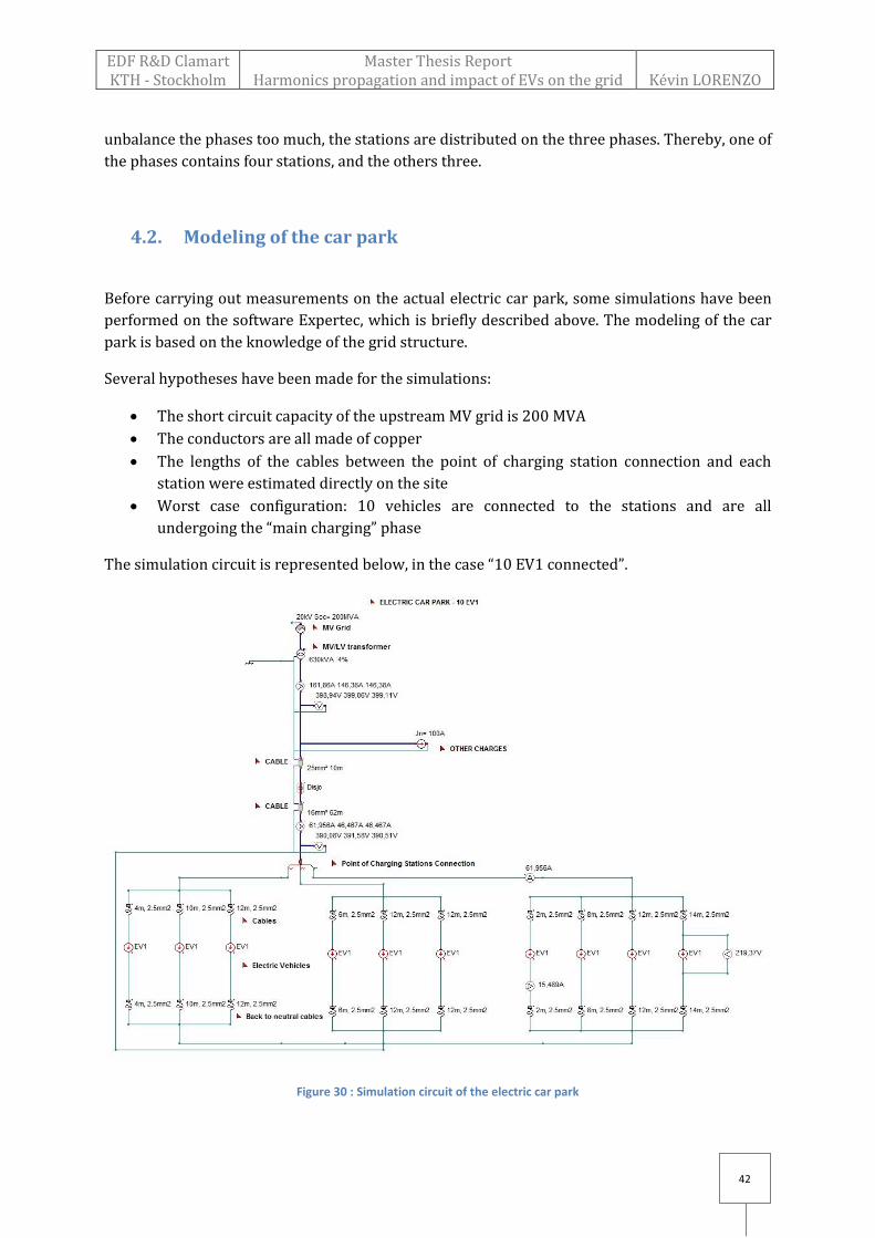
EDF R&D Clamart KTH - Stockholm
Master Thesis Report Harmonics propagation and impact of EVs on the grid
Kévin LORENZO
42
unbalance the phases too much, the stations are distributed on the three phases. Thereby, one of
the phases contains four stations, and the others three.
4.2. Modeling of the car park
Before carrying out measurements on the actual electric car park, some simulations have been
performed on the software Expertec, which is briefly described above. The modeling of the car
park is based on the knowledge of the grid structure.
Several hypotheses have been made for the simulations:
The short circuit capacity of the upstream MV grid is 200 MVA
The conductors are all made of copper
The lengths of the cables between the point of charging station connection and each
station were estimated directly on the site
Worst case configuration: 10 vehicles are connected to the stations and are all
undergoing the “main charging” phase
The simulation circuit is represented below, in the case “10 EV1 connected”.
Figure 30 : Simulation circuit of the electric car park
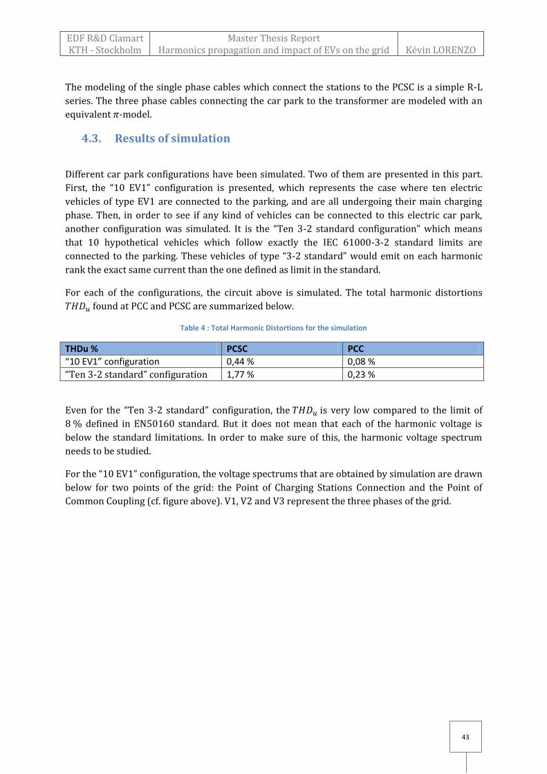
EDF R&D Clamart KTH - Stockholm
Master Thesis Report Harmonics propagation and impact of EVs on the grid
Kévin LORENZO
43
The modeling of the single phase cables which connect the stations to the PCSC is a simple R-L
series. The three phase cables connecting the car park to the transformer are modeled with an
equivalent -model.
4.3. Results of simulation
Different car park configurations have been simulated. Two of them are presented in this part.
First, the “10 EV1” configuration is presented, which represents the case where ten electric
vehicles of type EV1 are connected to the parking, and are all undergoing their main charging
phase. Then, in order to see if any kind of vehicles can be connected to this electric car park,
another configuration was simulated. It is the “Ten 3-2 standard configuration” which means
that 10 hypothetical vehicles which follow exactly the IEC 61000-3-2 standard limits are
connected to the parking. These vehicles of type “3-2 standard” would emit on each harmonic
rank the exact same current than the one defined as limit in the standard.
For each of the configurations, the circuit above is simulated. The total harmonic distortions
found at PCC and PCSC are summarized below.
Table 4 : Total Harmonic Distortions for the simulation
THDu % PCSC PCC
“10 EV1” configuration 0,44 % 0,08 %
“Ten 3-2 standard” configuration 1,77 % 0,23 %
Even for the “Ten 3-2 standard” configuration, the is very low compared to the limit of
8 % defined in EN50160 standard. But it does not mean that each of the harmonic voltage is
below the standard limitations. In order to make sure of this, the harmonic voltage spectrum
needs to be studied.
For the “10 EV1” configuration, the voltage spectrums that are obtained by simulation are drawn
below for two points of the grid: the Point of Charging Stations Connection and the Point of
Common Coupling (cf. figure above). V1, V2 and V3 represent the three phases of the grid.

EDF R&D Clamart KTH - Stockholm
Master Thesis Report Harmonics propagation and impact of EVs on the grid
Kévin LORENZO
44
Figure 31 : Mean voltage spectrum at the point of charging stations connection for 10 EV1
Figure 32 : Mean voltage spectrum at the point of common coupling for 10 EV1
The harmonic voltage levels are very low compared to the EN50160 limitations. Indeed, while
the harmonic voltages are 5 to 50 times lower at the PCSC than the EN50160 limitations, they
0
0,5
1
1,5
2
2,5
3
3,5
3 5 7 9 11 13 15 17 19 21 23 25 27 29 31 33 35 37 39
% o
f fu
nd
ame
nta
l
Harmonic rank
Voltage spectrum at PCSC (10 EV1)
V1
V2
V3
EN50160 standard
0
0,5
1
1,5
2
2,5
3
3 5 7 9 11 13 15 17 19 21 23 25 27 29 31 33 35 37 39
% o
f fu
nd
ame
nta
l
Harmonic rank
Voltage spectrum at PCC (10 EV1)
V1
V2
V3
EN50160 standard
EDF R&D Clamart KTH - Stockholm
Master Thesis Report Harmonics propagation and impact of EVs on the grid
Kévin LORENZO
45
are even hardly visible on the figure above for the PCC. The latter is the most important point
since the other charges of the LV grid are directly connected to this point.
Thus, even when 10 vehicles of type EV1 are connected at the same time to the electric car park,
the voltage is disturbed very little at the PCC. Since the vehicles that are today present on the
market have to comply with the IEC61000-3-2 limitations, if the “Ten 3-2 standard
configuration” does not create too high harmonic voltages, it means that theoretically every
vehicle could be connected to this parking. The results obtained for this configuration at PCC are
shown below.
Figure 33 : Mean voltage spectrum at the point of common coupling for "Ten 3-2 standard" configuration
With this « Ten 3-2 standard configuration », the harmonic voltage still comply with the
EN50160 standard about harmonic voltage limits. This means that, according to simulations,
every kind of electric vehicles absorbing 16 A during its charging, can be connected to this car
park, assuming that they respect the IEC61000-3-2 standard.
4.4. Measurements campaign
4.4.1. Method and measurement devices
The electrical grid layout of the 10 EV parking is given on the figure in section 4.1. On this grid,
all measurements have been taken right downstream the Point of Common Coupling (where the
other charges are connected), in order to study only the car park influence. Thus, the currents
which are measured at this point only concern the grid dedicated to the electric car park, but the
0
0,5
1
1,5
2
2,5
3
3,5
3 5 7 9 11 13 15 17 19 21 23 25 27 29 31 33 35 37 39
% o
f fu
nd
ame
nta
l
Harmonic rank
Voltage spectrum at PCC (Ten 3-2 standard)
V1
V2
V3
EN50160 standard
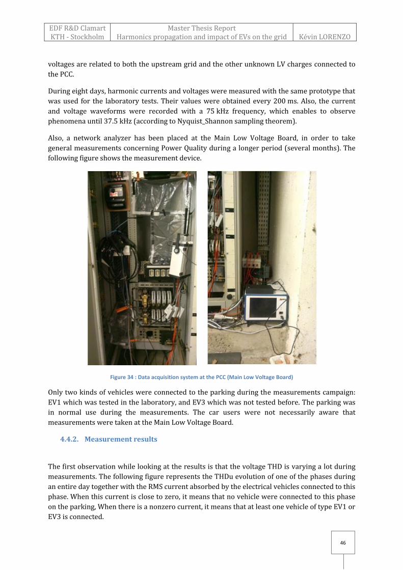
EDF R&D Clamart KTH - Stockholm
Master Thesis Report Harmonics propagation and impact of EVs on the grid
Kévin LORENZO
46
voltages are related to both the upstream grid and the other unknown LV charges connected to
the PCC.
During eight days, harmonic currents and voltages were measured with the same prototype that
was used for the laboratory tests. Their values were obtained every 200 ms. Also, the current
and voltage waveforms were recorded with a 75 kHz frequency, which enables to observe
phenomena until 37.5 kHz (according to Nyquist_Shannon sampling theorem).
Also, a network analyzer has been placed at the Main Low Voltage Board, in order to take
general measurements concerning Power Quality during a longer period (several months). The
following figure shows the measurement device.
Figure 34 : Data acquisition system at the PCC (Main Low Voltage Board)
Only two kinds of vehicles were connected to the parking during the measurements campaign:
EV1 which was tested in the laboratory, and EV3 which was not tested before. The parking was
in normal use during the measurements. The car users were not necessarily aware that
measurements were taken at the Main Low Voltage Board.
4.4.2. Measurement results
The first observation while looking at the results is that the voltage THD is varying a lot during
measurements. The following figure represents the THDu evolution of one of the phases during
an entire day together with the RMS current absorbed by the electrical vehicles connected to this
phase. When this current is close to zero, it means that no vehicle were connected to this phase
on the parking, When there is a nonzero current, it means that at least one vehicle of type EV1 or
EV3 is connected.
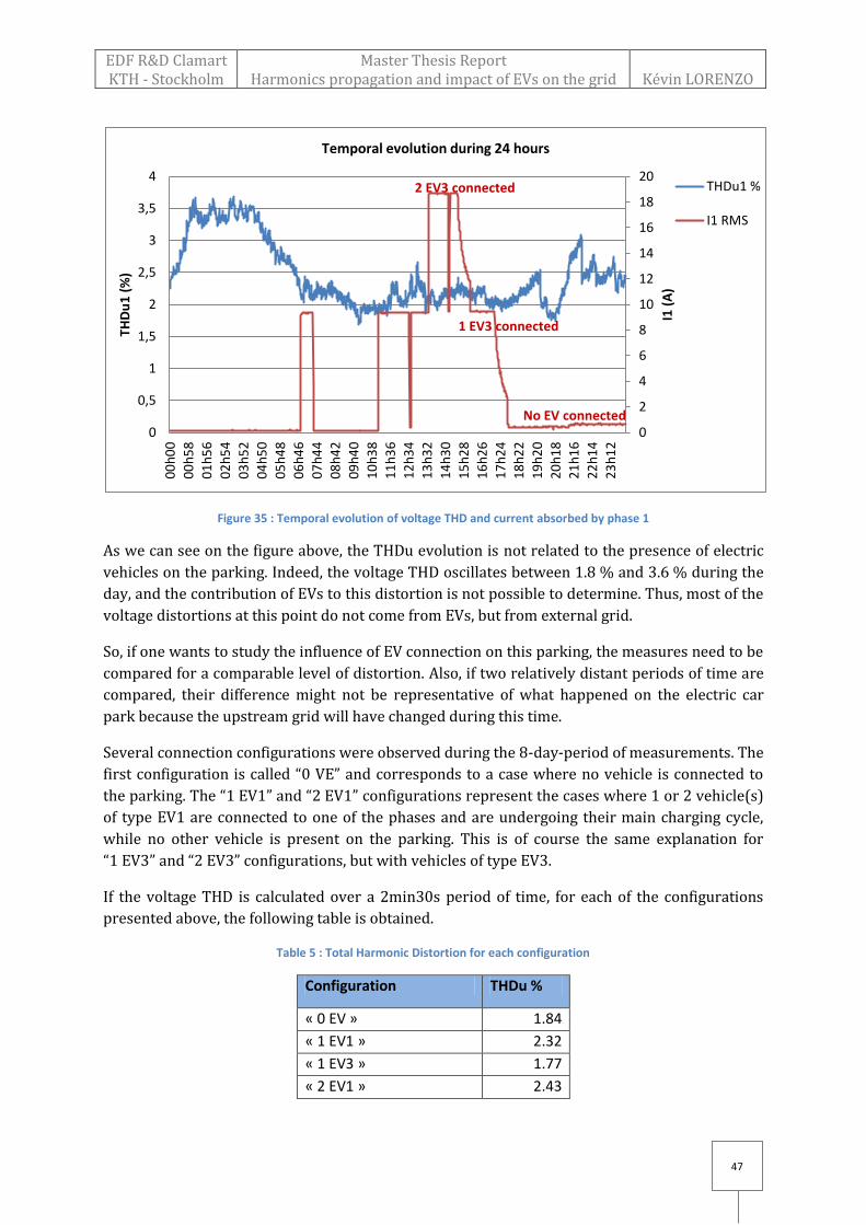
EDF R&D Clamart KTH - Stockholm
Master Thesis Report Harmonics propagation and impact of EVs on the grid
Kévin LORENZO
47
Figure 35 : Temporal evolution of voltage THD and current absorbed by phase 1
As we can see on the figure above, the THDu evolution is not related to the presence of electric
vehicles on the parking. Indeed, the voltage THD oscillates between 1.8 % and 3.6 % during the
day, and the contribution of EVs to this distortion is not possible to determine. Thus, most of the
voltage distortions at this point do not come from EVs, but from external grid.
So, if one wants to study the influence of EV connection on this parking, the measures need to be
compared for a comparable level of distortion. Also, if two relatively distant periods of time are
compared, their difference might not be representative of what happened on the electric car
park because the upstream grid will have changed during this time.
Several connection configurations were observed during the 8-day-period of measurements. The
first configuration is called “0 VE” and corresponds to a case where no vehicle is connected to
the parking. The “1 EV1” and “2 EV1” configurations represent the cases where 1 or 2 vehicle(s)
of type EV1 are connected to one of the phases and are undergoing their main charging cycle,
while no other vehicle is present on the parking. This is of course the same explanation for
“1 EV3” and “2 EV3” configurations, but with vehicles of type EV3.
If the voltage THD is calculated over a 2min30s period of time, for each of the configurations
presented above, the following table is obtained.
Table 5 : Total Harmonic Distortion for each configuration
Configuration THDu %
« 0 EV » 1.84
« 1 EV1 » 2.32
« 1 EV3 » 1.77
« 2 EV1 » 2.43
1 EV3 connected
2 EV3 connected
No EV connected 0
2
4
6
8
10
12
14
16
18
20
0
0,5
1
1,5
2
2,5
3
3,5
40
0h
00
00
h5
8
01
h5
6
02
h5
4
03
h5
2
04
h5
0
05
h4
8
06
h4
6
07
h4
4
08
h4
2
09
h4
0
10
h3
8
11
h3
6
12
h3
4
13
h3
2
14
h3
0
15
h2
8
16
h2
6
17
h2
4
18
h2
2
19
h2
0
20
h1
8
21
h1
6
22
h1
4
23
h1
2
I1 (
A)
THD
u1
(%
)
Temporal evolution during 24 hours
THDu1 %
I1 RMS

EDF R&D Clamart KTH - Stockholm
Master Thesis Report Harmonics propagation and impact of EVs on the grid
Kévin LORENZO
48
« 2 EV3 » 2.01
« 1 EV1 + 1 EV3 » 2.33
« 2 EV1 + 1 EV3 » 1.98
NB: The EN50160 standard defines a limit which is 8% for the THD of the feeding voltage on the
LV grid.
Given these results, there is no obvious correlation between the voltage THD and the presence of
electric vehicles on the grid. Indeed, the calculated THD for one EV3 present on the grid is even
lower than the one calculated for no vehicle on the park. However, it can be noticed that the
voltage THD is quite low, whatever the number of vehicles charging on the park.
It may also be appropriate to study the whole harmonic voltage spectrum. Indeed, the THD being
low does not mean that each of the harmonic voltage is below the EN50160 limit. The following
figures show the mean harmonic spectrum (calculated the same way as described in section 2.2)
for 0, 1 or 2 vehicle(s) of type EV1 (or EV3) connected to the grid.
Figure 36 : Influence of EV1 connection on the mean voltage spectrum
0
0,5
1
1,5
2
2,5
3 5 7 9 11 13 15 17 19 21 23 25 27 29 31 33 35 37 39
% o
f V
1
Harmonic rank
Voltage spectrum: 0, 1 ou 2 EV1 connected
0 EV
"1 EV1"
"2 EV1"
EN50160 standard

EDF R&D Clamart KTH - Stockholm
Master Thesis Report Harmonics propagation and impact of EVs on the grid
Kévin LORENZO
49
Figure 37 : Influence of EV3 connection on the mean voltage spectrum
NB: On the figures above, some of the standard limits are clipped, in order to see better the
influence of EVs connection.
So, observing each harmonic rank individually, harmonic voltages are way below the standard
limits for LV grids. Indeed, harmonic levels are always between 4 and 80 times lower than those
limits. This confirms the results of simulations presented above.
4.4.3. Observation: Behavior at higher frequencies
The measurements in the laboratory have shown that a particular behavior of electrical vehicles
can be observed at higher frequencies than the harmonic range [0 – 2 kHz]. So, it is important to
study perturbations in a higher range of frequency than the harmonic one. For this, it would
have been appropriate to use the measurements prototype allowing studies in the range of
frequency [2 – 150 kHz], which was already used for laboratory measurements. Unfortunately, it
was not possible to use it during the week when measures have been carried out.
However, it is still possible to study perturbations by applying Fourier transform to the recorded
waveforms. These waveforms have been recorded with a 75 kHz sampling frequency, which
means that phenomena can theoretically be observed until 37.5 kHz (Nyquist-Shannon
theorem). In order to avoid any aliasing problem, signals are studied until 30 kHz in this section.
This “high frequency” study is done by applying a Fourier transform to every 200 ms sample of
current and voltage waveforms. The temporal length of these samples (200 ms) gives a
spectrum with a 5 Hz step. Then a grouping of harmonics is done with a 200 Hz step in the range
[2 – 30 kHz] as follows:
0
0,5
1
1,5
2
2,5
3 5 7 9 11 13 15 17 19 21 23 25 27 29 31 33 35 37 39
% o
f V
1
Harmonic rank
Voltage spectrum: 0, 1 ou 2 EV3 connected
0 EV
"1 EV3"
"2 EV3"
EN50160 standard
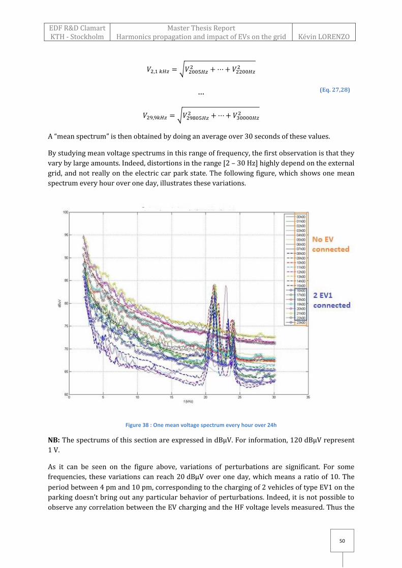
EDF R&D Clamart KTH - Stockholm
Master Thesis Report Harmonics propagation and impact of EVs on the grid
Kévin LORENZO
50
(Eq. 27,28)
√
…
√
A “mean spectrum” is then obtained by doing an average over 30 seconds of these values.
By studying mean voltage spectrums in this range of frequency, the first observation is that they
vary by large amounts. Indeed, distortions in the range [2 – 30 Hz] highly depend on the external
grid, and not really on the electric car park state. The following figure, which shows one mean
spectrum every hour over one day, illustrates these variations.
Figure 38 : One mean voltage spectrum every hour over 24h
NB: The spectrums of this section are expressed in dBµV. For information, 120 dBµV represent
1 V.
As it can be seen on the figure above, variations of perturbations are significant. For some
frequencies, these variations can reach 20 dBµV over one day, which means a ratio of 10. The
period between 4 pm and 10 pm, corresponding to the charging of 2 vehicles of type EV1 on the
parking doesn’t bring out any particular behavior of perturbations. Indeed, it is not possible to
observe any correlation between the EV charging and the HF voltage levels measured. Thus the
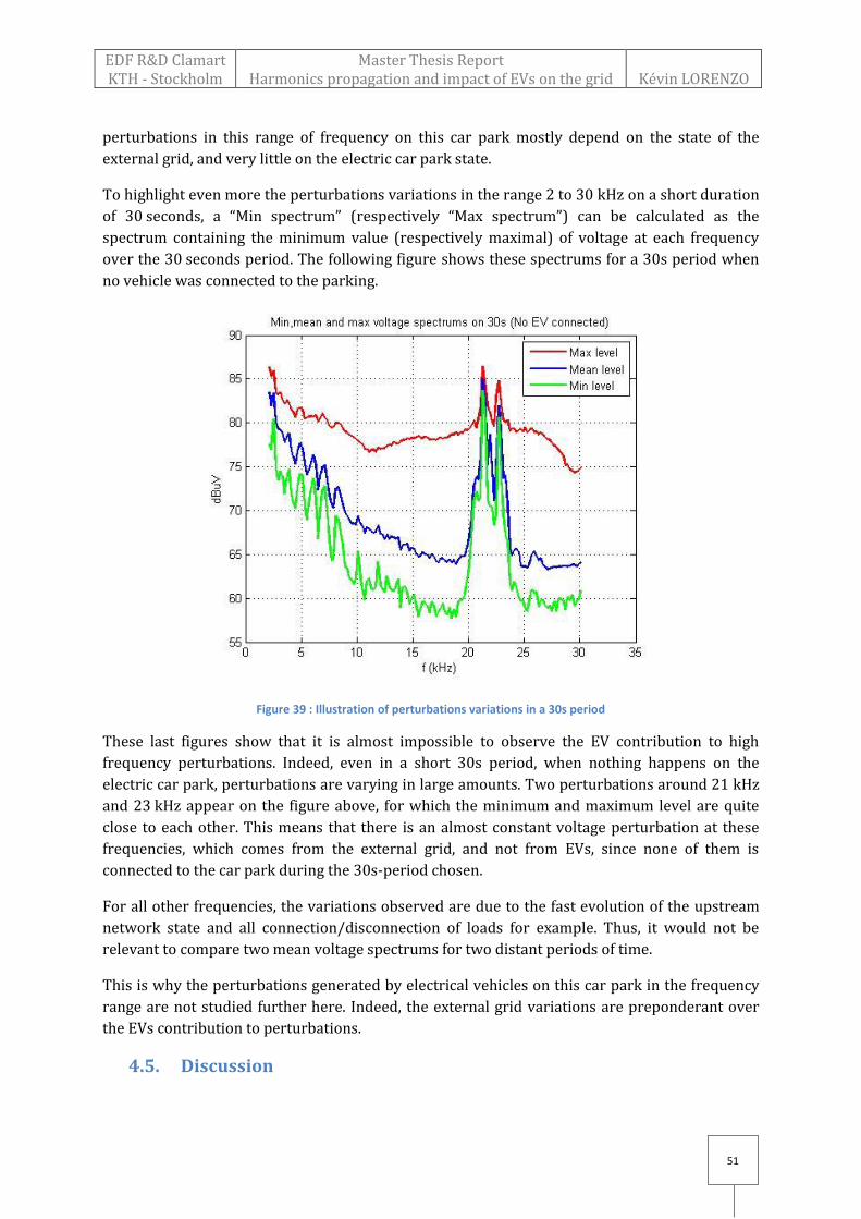
EDF R&D Clamart KTH - Stockholm
Master Thesis Report Harmonics propagation and impact of EVs on the grid
Kévin LORENZO
51
perturbations in this range of frequency on this car park mostly depend on the state of the
external grid, and very little on the electric car park state.
To highlight even more the perturbations variations in the range 2 to 30 kHz on a short duration
of 30 seconds, a “Min spectrum” (respectively “Max spectrum”) can be calculated as the
spectrum containing the minimum value (respectively maximal) of voltage at each frequency
over the 30 seconds period. The following figure shows these spectrums for a 30s period when
no vehicle was connected to the parking.
Figure 39 : Illustration of perturbations variations in a 30s period
These last figures show that it is almost impossible to observe the EV contribution to high
frequency perturbations. Indeed, even in a short 30s period, when nothing happens on the
electric car park, perturbations are varying in large amounts. Two perturbations around 21 kHz
and 23 kHz appear on the figure above, for which the minimum and maximum level are quite
close to each other. This means that there is an almost constant voltage perturbation at these
frequencies, which comes from the external grid, and not from EVs, since none of them is
connected to the car park during the 30s-period chosen.
For all other frequencies, the variations observed are due to the fast evolution of the upstream
network state and all connection/disconnection of loads for example. Thus, it would not be
relevant to compare two mean voltage spectrums for two distant periods of time.
This is why the perturbations generated by electrical vehicles on this car park in the frequency
range are not studied further here. Indeed, the external grid variations are preponderant over
the EVs contribution to perturbations.
4.5. Discussion
EDF R&D Clamart KTH - Stockholm
Master Thesis Report Harmonics propagation and impact of EVs on the grid
Kévin LORENZO
52
From laboratory measurements to onsite measurements, passing through modeling and
simulations, the study enabled to show several things about Electrical Vehicles impact on power
quality.
First, the vehicles models that were used for measurements do not seem to generate harmonic
voltages which would cause problems on the power quality of the surrounding grid. Indeed,
individual testing of vehicles as well as onsite measurements show that harmonic voltages
coming from EV connections stay quite low. This observation especially applies to the 10-
electric-car-park that has been subject to studies. Moreover, simulations have shown that any
kind of electric vehicle, assuming that it respects the standards about harmonics current
emission, could be connected to this car park without disturbing voltage by large amounts.
However, as it is by shown multiple laboratory testing, harmonic voltages can be significantly
increased by EV connections if the grid is not strong enough, which means that the short circuit
impedance of upstream grid is too high. So the previous result concerning the 10 EV park is valid
for this park, but might not be valid for every electric car park containing 10 charging stations. It
indeed depends on the upstream grid strength.
Also, an observation from laboratory measurements is that EV connection can bring
perturbations in frequency ranges higher than the harmonic one (0–2 kHz). The problem with
high frequency perturbations (2-150 kHz), is that no standard currently limits them and that one
cannot assure that sensitive equipment connected to the grid will not be affected..It is also hard
to study perturbations in this range of frequency, since they vary not only in large amounts but
also very fast, depending on the state of the network.
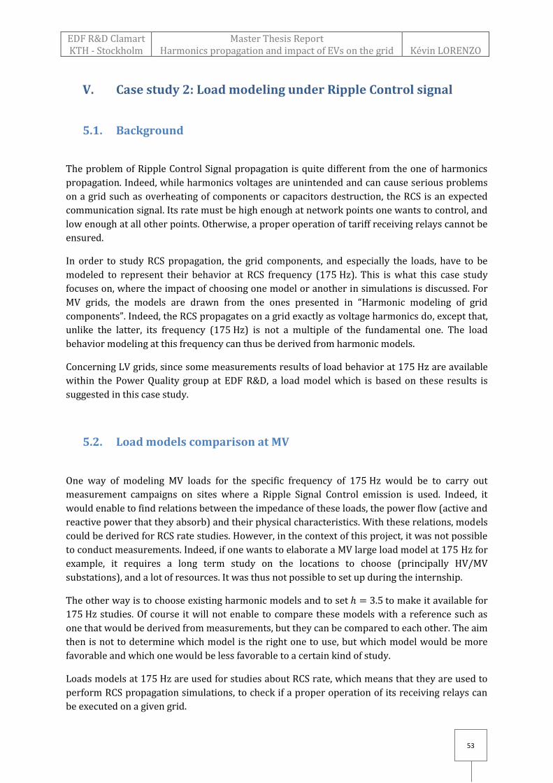
EDF R&D Clamart KTH - Stockholm
Master Thesis Report Harmonics propagation and impact of EVs on the grid
Kévin LORENZO
53
V. Case study 2: Load modeling under Ripple Control signal
5.1. Background
The problem of Ripple Control Signal propagation is quite different from the one of harmonics
propagation. Indeed, while harmonics voltages are unintended and can cause serious problems
on a grid such as overheating of components or capacitors destruction, the RCS is an expected
communication signal. Its rate must be high enough at network points one wants to control, and
low enough at all other points. Otherwise, a proper operation of tariff receiving relays cannot be
ensured.
In order to study RCS propagation, the grid components, and especially the loads, have to be
modeled to represent their behavior at RCS frequency (175 Hz). This is what this case study
focuses on, where the impact of choosing one model or another in simulations is discussed. For
MV grids, the models are drawn from the ones presented in “Harmonic modeling of grid
components”. Indeed, the RCS propagates on a grid exactly as voltage harmonics do, except that,
unlike the latter, its frequency (175 Hz) is not a multiple of the fundamental one. The load
behavior modeling at this frequency can thus be derived from harmonic models.
Concerning LV grids, since some measurements results of load behavior at 175 Hz are available
within the Power Quality group at EDF R&D, a load model which is based on these results is
suggested in this case study.
5.2. Load models comparison at MV
One way of modeling MV loads for the specific frequency of 175 Hz would be to carry out
measurement campaigns on sites where a Ripple Signal Control emission is used. Indeed, it
would enable to find relations between the impedance of these loads, the power flow (active and
reactive power that they absorb) and their physical characteristics. With these relations, models
could be derived for RCS rate studies. However, in the context of this project, it was not possible
to conduct measurements. Indeed, if one wants to elaborate a MV large load model at 175 Hz for
example, it requires a long term study on the locations to choose (principally HV/MV
substations), and a lot of resources. It was thus not possible to set up during the internship.
The other way is to choose existing harmonic models and to set to make it available for
175 Hz studies. Of course it will not enable to compare these models with a reference such as
one that would be derived from measurements, but they can be compared to each other. The aim
then is not to determine which model is the right one to use, but which model would be more
favorable and which one would be less favorable to a certain kind of study.
Loads models at 175 Hz are used for studies about RCS rate, which means that they are used to
perform RCS propagation simulations, to check if a proper operation of its receiving relays can
be executed on a given grid.
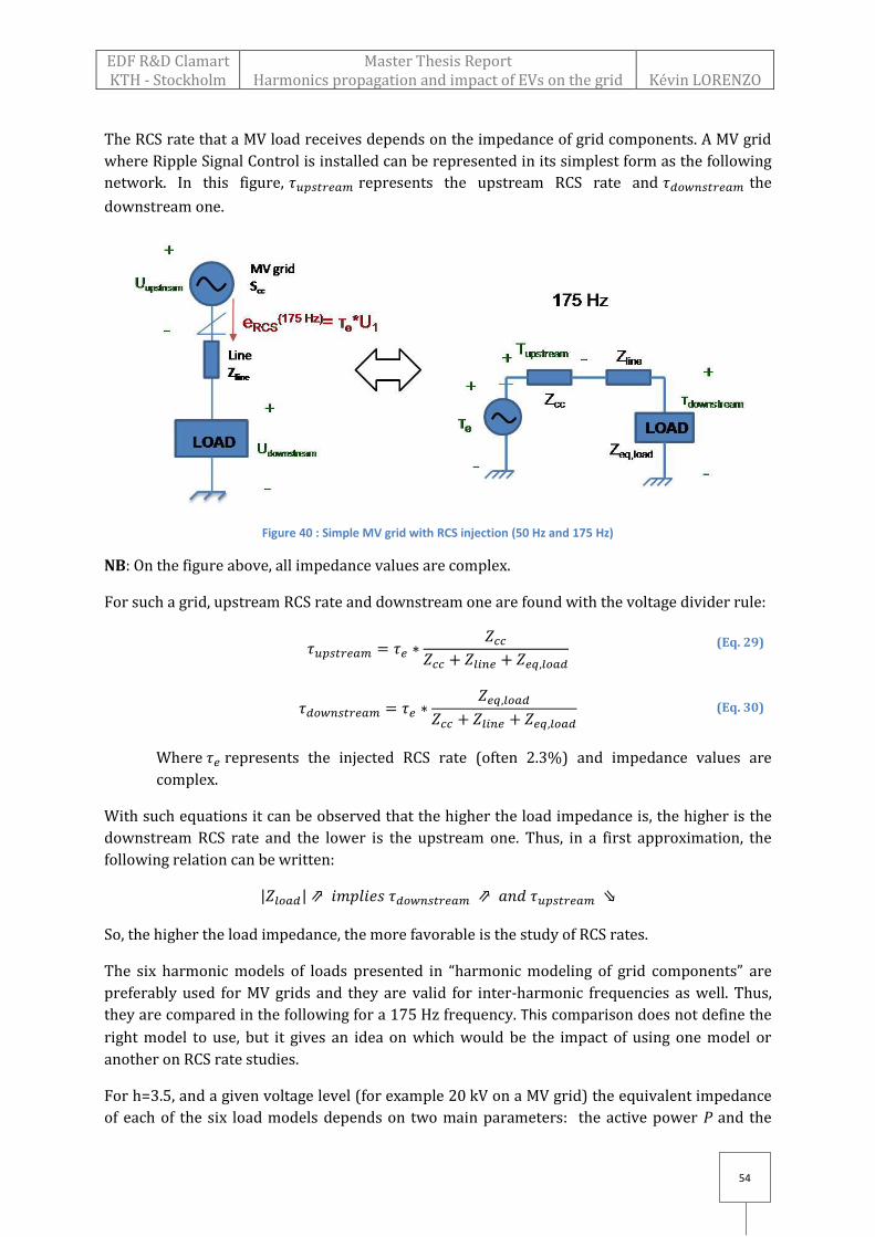
EDF R&D Clamart KTH - Stockholm
Master Thesis Report Harmonics propagation and impact of EVs on the grid
Kévin LORENZO
54
(Eq. 29)
(Eq. 30)
The RCS rate that a MV load receives depends on the impedance of grid components. A MV grid
where Ripple Signal Control is installed can be represented in its simplest form as the following
network. In this figure, represents the upstream RCS rate and the
downstream one.
Figure 40 : Simple MV grid with RCS injection (50 Hz and 175 Hz)
NB: On the figure above, all impedance values are complex.
For such a grid, upstream RCS rate and downstream one are found with the voltage divider rule:
Where represents the injected RCS rate (often 2.3%) and impedance values are
complex.
With such equations it can be observed that the higher the load impedance is, the higher is the
downstream RCS rate and the lower is the upstream one. Thus, in a first approximation, the
following relation can be written:
| |
So, the higher the load impedance, the more favorable is the study of RCS rates.
The six harmonic models of loads presented in “harmonic modeling of grid components” are
preferably used for MV grids and they are valid for inter-harmonic frequencies as well. Thus,
they are compared in the following for a 175 Hz frequency. This comparison does not define the
right model to use, but it gives an idea on which would be the impact of using one model or
another on RCS rate studies.
For h=3.5, and a given voltage level (for example 20 kV on a MV grid) the equivalent impedance
of each of the six load models depends on two main parameters: the active power P and the
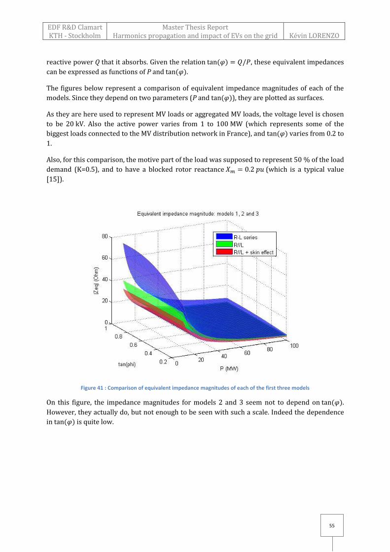
EDF R&D Clamart KTH - Stockholm
Master Thesis Report Harmonics propagation and impact of EVs on the grid
Kévin LORENZO
55
reactive power Q that it absorbs. Given the relation ( ) , these equivalent impedances
can be expressed as functions of P and ( ).
The figures below represent a comparison of equivalent impedance magnitudes of each of the
models. Since they depend on two parameters (P and ( )), they are plotted as surfaces.
As they are here used to represent MV loads or aggregated MV loads, the voltage level is chosen
to be 20 kV. Also the active power varies from 1 to 100 MW (which represents some of the
biggest loads connected to the MV distribution network in France), and ( ) varies from 0.2 to
1.
Also, for this comparison, the motive part of the load was supposed to represent 50 % of the load
demand (K=0.5), and to have a blocked rotor reactance (which is a typical value
[15]).
Figure 41 : Comparison of equivalent impedance magnitudes of each of the first three models
On this figure, the impedance magnitudes for models 2 and 3 seem not to depend on ( ).
However, they actually do, but not enough to be seen with such a scale. Indeed the dependence
in ( ) is quite low.
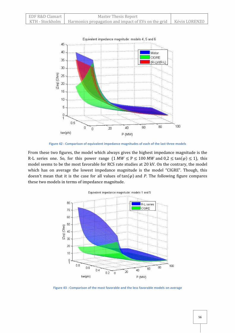
EDF R&D Clamart KTH - Stockholm
Master Thesis Report Harmonics propagation and impact of EVs on the grid
Kévin LORENZO
56
Figure 42 : Comparison of equivalent impedance magnitudes of each of the last three models
From these two figures, the model which always gives the highest impedance magnitude is the
R-L series one. So, for this power range ( and ( ) ), this
model seems to be the most favorable for RCS rate studies at 20 kV. On the contrary, the model
which has on average the lowest impedance magnitude is the model “CIGRE”. Though, this
doesn’t mean that it is the case for all values of ( ) and P. The following figure compares
these two models in terms of impedance magnitude.
Figure 43 : Comparison of the most favorable and the less favorable models on average
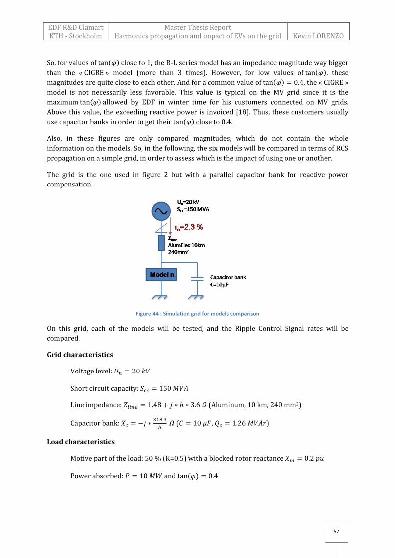
EDF R&D Clamart KTH - Stockholm
Master Thesis Report Harmonics propagation and impact of EVs on the grid
Kévin LORENZO
57
So, for values of ( ) close to 1, the R-L series model has an impedance magnitude way bigger
than the « CIGRE » model (more than 3 times). However, for low values of ( ), these
magnitudes are quite close to each other. And for a common value of ( ) , the « CIGRE »
model is not necessarily less favorable. This value is typical on the MV grid since it is the
maximum ( ) allowed by EDF in winter time for his customers connected on MV grids.
Above this value, the exceeding reactive power is invoiced [18]. Thus, these customers usually
use capacitor banks in order to get their ( ) close to 0.4.
Also, in these figures are only compared magnitudes, which do not contain the whole
information on the models. So, in the following, the six models will be compared in terms of RCS
propagation on a simple grid, in order to assess which is the impact of using one or another.
The grid is the one used in figure 2 but with a parallel capacitor bank for reactive power
compensation.
Figure 44 : Simulation grid for models comparison
On this grid, each of the models will be tested, and the Ripple Control Signal rates will be
compared.
Grid characteristics
Voltage level:
Short circuit capacity:
Line impedance: (Aluminum, 10 km, 240 mm2)
Capacitor bank:
( , )
Load characteristics
Motive part of the load: 50 % (K=0.5) with a blocked rotor reactance
Power absorbed: and ( )
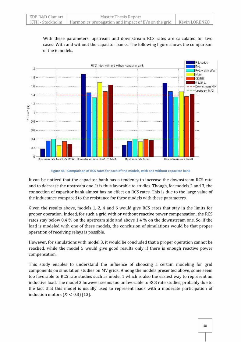
EDF R&D Clamart KTH - Stockholm
Master Thesis Report Harmonics propagation and impact of EVs on the grid
Kévin LORENZO
58
With these parameters, upstream and downstream RCS rates are calculated for two
cases: With and without the capacitor banks. The following figure shows the comparison
of the 6 models.
Figure 45 : Comparison of RCS rates for each of the models, with and without capacitor bank
It can be noticed that the capacitor bank has a tendency to increase the downstream RCS rate
and to decrease the upstream one. It is thus favorable to studies. Though, for models 2 and 3, the
connection of capacitor bank almost has no effect on RCS rates. This is due to the large value of
the inductance compared to the resistance for these models with these parameters.
Given the results above, models 1, 2, 4 and 6 would give RCS rates that stay in the limits for
proper operation. Indeed, for such a grid with or without reactive power compensation, the RCS
rates stay below 0.4 % on the upstream side and above 1.4 % on the downstream one. So, if the
load is modeled with one of these models, the conclusion of simulations would be that proper
operation of receiving relays is possible.
However, for simulations with model 3, it would be concluded that a proper operation cannot be
reached, while the model 5 would give good results only if there is enough reactive power
compensation.
This study enables to understand the influence of choosing a certain modeling for grid
components on simulation studies on MV grids. Among the models presented above, some seem
too favorable to RCS rate studies such as model 1 which is also the easiest way to represent an
inductive load. The model 3 however seems too unfavorable to RCS rate studies, probably due to
the fact that this model is usually used to represent loads with a moderate participation of
induction motors ( ) [13].

EDF R&D Clamart KTH - Stockholm
Master Thesis Report Harmonics propagation and impact of EVs on the grid
Kévin LORENZO
59
(Eq. 31)
(Eq. 32)
5.3. From MV model to LV model
The models discussed in the previous section mostly concerns MV grids. However, there are no
models available to represent a Low Voltage load at ripple frequency (175 Hz). The following
will show the method that was used in order to derive one model of LV RCS load based on the
results of measurement on LV grid.
In 2008, a measurement campaign was carried out by the EDF Power Quality group, on a dozen
MV/LV substations where Ripple Control Signal was operating. The aim of these measurements
was to characterize the behavior of a typical aggregate LV load by trying to link its impedance at
175 Hz, to its electrical quantities at fundamental frequency. Indeed, if simple relations are
found between them, a LV load model such as the ones presented before can be derived. An
aggregate LV load is defined [19] as all LV loads fed through the same circuit breaker at the
MV/LV substation.
The results of these measurements enabled, by using a linear regression method, to find a linear
relation between the impedance at 175 Hz of an aggregate LV load, and its impedance at 50 Hz.
Due to confidentiality reasons, coefficients values are not given in this report, but the form is:
| | | |
It was also determined that the argument of this impedance was not related to reactive power
absorbed, but in most of the cases its value was negative. This means that the typical aggregate
LV load measured had a capacitive tendency at 175 Hz. This is probably due to the capacitive
behavior of cables and also all capacitive applications on LV networks. As most of the argument
values are contained in a relatively small range around a certain negative value of angle, it was
chosen to take this value as representative of a typical LV 175 Hz impedance, so that:
( )
Then, knowing both the magnitude and the argument behavior, it is possible to suggest a model
for aggregate RCS loads on LV grid.
In the context of this thesis, it was chosen to suggest a model inspired from the one
recommended by the CIGRE, but to adjust it in order to make it respect the relations coming
from LV measurements. This model will be called “LV model”.
Figure 46 : "LV Model" of a typical aggregate load
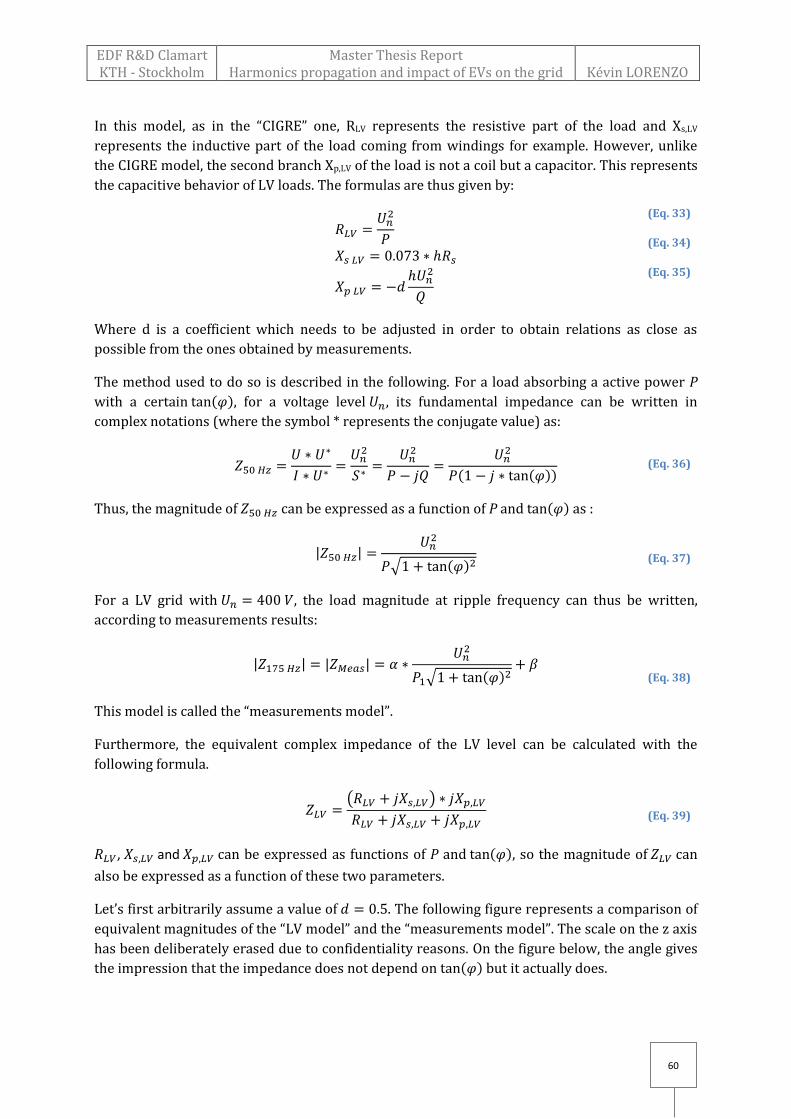
EDF R&D Clamart KTH - Stockholm
Master Thesis Report Harmonics propagation and impact of EVs on the grid
Kévin LORENZO
60
(Eq. 33)
(Eq. 34)
(Eq. 35)
(Eq. 36)
(Eq. 37)
(Eq. 38)
(Eq. 39)
In this model, as in the “CIGRE” one, RLV represents the resistive part of the load and Xs,LV
represents the inductive part of the load coming from windings for example. However, unlike
the CIGRE model, the second branch Xp,LV of the load is not a coil but a capacitor. This represents
the capacitive behavior of LV loads. The formulas are thus given by:
Where d is a coefficient which needs to be adjusted in order to obtain relations as close as
possible from the ones obtained by measurements.
The method used to do so is described in the following. For a load absorbing a active power P
with a certain ( ), for a voltage level , its fundamental impedance can be written in
complex notations (where the symbol * represents the conjugate value) as:
( ( ))
Thus, the magnitude of can be expressed as a function of P and ( ) as :
| |
√ ( )
For a LV grid with , the load magnitude at ripple frequency can thus be written,
according to measurements results:
| | | |
√ ( )
This model is called the “measurements model”.
Furthermore, the equivalent complex impedance of the LV level can be calculated with the
following formula.
( )
, and can be expressed as functions of P and ( ), so the magnitude of can
also be expressed as a function of these two parameters.
Let’s first arbitrarily assume a value of . The following figure represents a comparison of
equivalent magnitudes of the “LV model” and the “measurements model”. The scale on the z axis
has been deliberately erased due to confidentiality reasons. On the figure below, the angle gives
the impression that the impedance does not depend on ( ) but it actually does.

EDF R&D Clamart KTH - Stockholm
Master Thesis Report Harmonics propagation and impact of EVs on the grid
Kévin LORENZO
61
(Eq. 40)
Figure 47 : Magnitudes comparison for "LV model" and "Measurements model" (d=0.5)
What needs to be done now is to adjust the parameter d of the LV model in order to make its
equivalent impedance closer to the “Measurement model” one. Concretely, this means adjusting
the parameter d to make the red surface as close as possible to the blue one.
The chosen intervals of variations for P and ( ) are:
( )
The parameter d can first be adjusted by hand to try to make the surfaces closer. But in order to
get them more precisely, a numerical method inspired from the method of least squares is used
here. It consists in minimizing, by making the parameter d vary, the following squared error:
∑ ∑ (| |
| |
)
( )
( )
By minimization of this quantity, a certain value of d is found. With this value, the comparison of
equivalent magnitudes of the “LV model” and the “measurements model” is plotted below:

EDF R&D Clamart KTH - Stockholm
Master Thesis Report Harmonics propagation and impact of EVs on the grid
Kévin LORENZO
62
Figure 48 : Magnitudes comparison for "LV model" and "Measurements model" (Optimized d)
For a common value of ( ) , the first “LV model”, the adjusted “LV model” and the
“Measurements model” magnitudes are compared below. This is actually a sectional view of the
two previous figures.
Figure 49 : ( ) , magnitudes comparison for "LV model" and "Measurements model" (Optimized d)
As it can be seen on the figure above, for ( ) which is a common value, the adjusted LV
model obtained is very close to the one directly derived from measurements in terms of
EDF R&D Clamart KTH - Stockholm
Master Thesis Report Harmonics propagation and impact of EVs on the grid
Kévin LORENZO
63
equivalent impedance magnitude. However, for lower values of ( ), the load impedance
magnitude would be overestimated by using “LV model”, while it would be underestimated for
higher values.
Concerning load impedance argument, this model gives a negative value, which corresponds to
the expected capacitive behavior.
Figure 50: Argument of the adjusted "LV model" equivalent impedance
The values observed are a bit high compared to the ones expected. However, the “LV model”
provides a good approximation of the behavior of a typical aggregate LV load at 175 Hz,
especially for ( ) close to 0.4.
5.4. Grid reduction
While the two previous sections focused on the ways of modeling loads, this one addresses the
more general problem of grid modeling and presents a broadening to the study. Indeed, when
one wants to study Ripple Control Signal propagation, a choice needs to be done between
modeling each of the components of the whole detailed grid and gathering components in order
to make aggregate models. When used into simulation tools, the detailed grid would provide
more precise results, while the reduced one would decrease processing time and make the input
of information easier.
The following study focuses on which is the impact of using aggregate MV load models instead of
using detailed networks where each MV load is modeled separately.
The first thing to notice is that, when the impedance of cables is neglected, if the same model is
used to represent the aggregate load or each of the MV loads, the exact same impedance at
175 Hz is found at the PCC. The figure below shows the equivalence of impedance between the
detailed network where each of the nodes is represented by a model, and the aggregated one
where this same model represents the aggregation of all nodes.
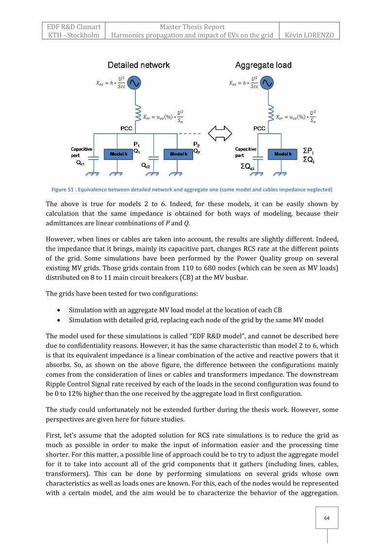
EDF R&D Clamart KTH - Stockholm
Master Thesis Report Harmonics propagation and impact of EVs on the grid
Kévin LORENZO
64
Figure 51 : Equivalence between detailed network and aggregate one (same model and cables impedance neglected)
The above is true for models 2 to 6. Indeed, for these models, it can be easily shown by
calculation that the same impedance is obtained for both ways of modeling, because their
admittances are linear combinations of P and Q.
However, when lines or cables are taken into account, the results are slightly different. Indeed,
the impedance that it brings, mainly its capacitive part, changes RCS rate at the different points
of the grid. Some simulations have been performed by the Power Quality group on several
existing MV grids. Those grids contain from 110 to 680 nodes (which can be seen as MV loads)
distributed on 8 to 11 main circuit breakers (CB) at the MV busbar.
The grids have been tested for two configurations:
Simulation with an aggregate MV load model at the location of each CB
Simulation with detailed grid, replacing each node of the grid by the same MV model
The model used for these simulations is called “EDF R&D model”, and cannot be described here
due to confidentiality reasons. However, it has the same characteristic than model 2 to 6, which
is that its equivalent impedance is a linear combination of the active and reactive powers that it
absorbs. So, as shown on the above figure, the difference between the configurations mainly
comes from the consideration of lines or cables and transformers impedance. The downstream
Ripple Control Signal rate received by each of the loads in the second configuration was found to
be 0 to 12% higher than the one received by the aggregate load in first configuration.
The study could unfortunately not be extended further during the thesis work. However, some
perspectives are given here for future studies.
First, let’s assume that the adopted solution for RCS rate simulations is to reduce the grid as
much as possible in order to make the input of information easier and the processing time
shorter. For this matter, a possible line of approach could be to try to adjust the aggregate model
for it to take into account all of the grid components that it gathers (including lines, cables,
transformers). This can be done by performing simulations on several grids whose own
characteristics as well as loads ones are known. For this, each of the nodes would be represented
with a certain model, and the aim would be to characterize the behavior of the aggregation.
EDF R&D Clamart KTH - Stockholm
Master Thesis Report Harmonics propagation and impact of EVs on the grid
Kévin LORENZO
65
Another way to do so could be to realize measurements at MV busbar of several known
networks.
If the detailed modeling is found to be better for RCS rate simulations, the question would then
be how to model each node of the grid. One suggestion is to develop a model which could be
adjusted to each load by including parameters. The latter would enable to split the load in
several parts with, for example, A% of motive part, B% of resistive part, C% of capacitive part,
and so on. For this, measurements as well as simulations would be necessary.
5.5. Discussion
This case study is based on the fact that the Ripple Control Signal propagation acts the same way
as harmonics propagation does. While grid components such as cables, transformers or sources
can be simply modeled by their harmonic models taken at 175 Hz, the modeling of other
components such as loads, which can be of all sorts, needs a particular attention.
As it can be seen in the second part of this case study concerning MV load modeling, the choice of
one model or another in simulation tools can have great impact on studies. Some would be
favorable to RCS rate studies while others would be unfavorable. Measurements on actual grids
can give information on the most representative load model. This is why the third part of this
case study, which is about LV load model at 175 Hz, relies mainly on measurements results. The
model that is suggested in this part is satisfactory for ( ) close to 0.4, but not really for other
values.
The last part of this case study is a broadening, and concerns the problem of grid reduction in
simulation tools. It provides lines of approach for future studies about aggregate load models.
EDF R&D Clamart KTH - Stockholm
Master Thesis Report Harmonics propagation and impact of EVs on the grid
Kévin LORENZO
66
VI. Conclusion
Two different kinds of studies are led in this report: one about the harmonic impact of an electric
car park on the surrounding electrical grid, and the other one about the load modeling at Ripple
Control Signal frequency. Although those studies seem quite independent, they both concern the
propagation of (inter)harmonic voltages on the electricity distribution network.
The main result of the part concerning Electric Vehicles is that no practical problems appear to
occur with the use of the 10-electric-car park studied. For both simulations and measurements
(onsite or in laboratory), harmonic voltages stay relatively low. However, multiple testing on
four vehicles in laboratory has shown that disturbing harmonic voltage levels might appear on
the local grid, when several cars are connected simultaneously. This depends on the upstream
grid impedance. Indeed, the weaker the grid is (i.e. the higher its upstream impedance is), the
higher are harmonic voltages generated by each of the car connected. This gives the information
that special precautions need to be taken if an electric car park is connected to the grid quite far
from the MV substation. Though, it is not possible to recommend a maximum number of cars
connected on a parking with the measurements performed only. Also, the study shows that more
investigations need to be carried out in higher frequency ranges. Indeed, for perturbations
appearing in the range [2-150 kHz], one cannot assure that sensitive equipment connected to
the grid will not be affected and no standard is currently available to limit emissions or
absorptions.
In the second part concerning Ripple Control Signal propagation, the study shows that there can
be great impacts on simulation studies of using one model or another to represent grid
components. One model of LV load at ripple frequency based on recent measurements results is
presented here. However, this one is valid for quite a narrow range of reactive power rate, and
needs to be reinforced by other measurements.
EDF R&D Clamart KTH - Stockholm
Master Thesis Report Harmonics propagation and impact of EVs on the grid
Kévin LORENZO
67
References
[1] EDF. [Online]. http://www.edf.com/the-edf-group-42667.html
[2] L. Berthet (Senior Expert in Power Quality), "EDF R&D Lecture on Power quality (Internal
reports)," , 2013.
[3] Schneider Electric - Ph. Ferracci, "Cahier technique n°199 - Power Quality," 1999.
[4] T. Deflandre - P.Mauras, "Les cahiers de l'ingénierie" Harmonics on industrial and tertiary
networks (in French)., 1997.
[5] International Standard IEC 61000-3-2, Electromagnetic compatibility (EMC) – Part 3-2: Limits –
Limits for harmonic current emissions (equipment input current ≤16 A per phase)., 2009.
[6] European Standard EN50160, Voltage characteristics of electricity supplied by public electricity
networks., 2011.
[7] International Standard IEC61000-4-7, "Part 4-7: Testing and measurement techniques – General
guide on harmonics and interharmonics measurements and instrumentation, for power supply
systems and equipment connected thereto," 2009.
[8] ECPE Workshop, "State of the art of batteries and charging concepts," Valencia, 2011.
[9] Schneider Electric, "EVlink - Electric Vehicle charging solutions," Guide 2013.
[10] ST Microelectronics - Reiner Schwartz, "Battery charging strategies," , 2010.
[11] T. Deflandre, CIGRE 36.05 A. Robert, "Guide for assessing the network harmonic impedance,"
Electra 167, 1996.
[12] Hadi Saadat, Power System Analysis Third Edition.: PSA Publishing, 2010.
[13] IEEE Task force on Harmonic Modeling and Simulation, "Impact of Aggregate Linear Load
Modeling on Harmonic Analysis: A Comparison of Common Practice and Analytical Models,"
2003.
[14] IEEE Task Force on Harmonics Modeling and Simulation, "Modeling and Simulation of the
Propagation of Harmonics in Electric Power Networks," Part 1 : Concepts, models and simulation
techniques 1996.
[15] R. Natarajan, Computer-aided Power System Analysis. p.55, 2002.
[16] CIGRE Working Group 36.05, "Harmonics, characteristic parameters, methods of study,
estimates of existing values in the network," Electra 77, pp. 35-54, 1981.
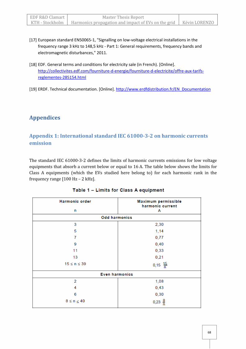
EDF R&D Clamart KTH - Stockholm
Master Thesis Report Harmonics propagation and impact of EVs on the grid
Kévin LORENZO
68
[17] European standard EN50065-1, "Signalling on low-voltage electrical installations in the
frequency range 3 kHz to 148,5 kHz - Part 1: General requirements, frequency bands and
electromagnetic disturbances," 2011.
[18] EDF. General terms and conditions for electricity sale (in French). [Online].
http://collectivites.edf.com/fourniture-d-energie/fourniture-d-electricite/offre-aux-tarifs-
reglementes-285154.html
[19] ERDF. Technical documentation. [Online]. http://www.erdfdistribution.fr/EN_Documentation
Appendices
Appendix 1: International standard IEC 61000-3-2 on harmonic currents
emission
The standard IEC 61000-3-2 defines the limits of harmonic currents emissions for low voltage
equipments that absorb a current below or equal to 16 A. The table below shows the limits for
Class A equipments (which the EVs studied here belong to) for each harmonic rank in the
frequency range [100 Hz – 2 kHz].

EDF R&D Clamart KTH - Stockholm
Master Thesis Report Harmonics propagation and impact of EVs on the grid
Kévin LORENZO
69
Appendix 2: European standard EN50160 on harmonic voltages emission
The standard EN50160 defines the characteristics of the supplied voltage on the low and
medium voltage distribution system. In normal conditions, for each one-week-period, 95 % of
the average value on 10 minutes of harmonic voltages (RMS value) must not be greater than the
values indicated below.
Also, the THD of the supplied voltage (including all harmonics up to the 40th rank) must be
below 8%.
Harmonic voltages expressed in % of the fundamental voltage Odd harmonics Even harmonics
Not multiple of 3 Multiple of 3 Rank h Relative
magnitude Rank h Relative
magnitude Rank h Relative
magnitude 5 6 % 3 5 % 2 2 % 7 5% 9 1.5 % 4 1 %
11 3.5 % 15 0.5 % 6…24 0.5 % 13 3 % 21 0.5 % 17 2 % 19 1.5 % 23 1.5 % 25 1.5 %
Values corresponding to harmonics of a higher order than 25 are very unpredictable by virtue of resonance effects.