Evolving Comparative Advantage in International

Shipbuilding During the Transition from Wood to Steel ∗

W. Walker HanlonNYU Stern School of Business & NBER

PRELIMINARY

July 20, 2017

Abstract

Can temporary initial input cost advantages have a long-run impact on thespatial distribution of production and trade? I study this question in the con-text of the international shipbuilding industry during the transition from woodto metal ship production (1850-1912). Input price advantages gave Britain anearly lead in metal shipbuilding, while the U.S. and Canada specialized in woodship production. However, after 1890 Britain’s initial price advantages disap-peared. By comparing production patterns on the Atlantic Coast of NorthAmerica, which faced British competition, to the Great Lakes, which wereisolated from competition, I show that competition from initially advantagedforeign firms substantially reduced the ability of North American producers totransition to metal ship production. Government protection and support mod-erated these effects for some Atlantic Coast producers, allowing them to survivethe demise of wood shipbuilding. I also provide evidence that the mechanismdriving the persistence of Britain’s lead was the development of large pools ofskilled craft workers. These results shed light on the role of past conditions ininfluencing current production and trade patterns, with implications for mod-ern debates over the use of industrial policy and tariff protection.

∗I am grateful to the International Economics Section at Princeton for support and advice whilewriting this paper. I thank Philip Ager, Leah Boustan, Stephen Broadberry, Capser Worm Hansen,Ian Kaey, Petra Moser, Henry Overman, Ariel Pakes and Jean-Laurent Rosenthal and seminarparticipants at Caltech, Copenhagen, Princeton, Warwick and NYU Stern for helpful comments.Meng Xu and Anna Sudol provided excellent research assistance. Funding was provided by a ColeGrant from the Economic History Association, the Hellman Fellowship at UCLA, a research grantfrom UCLA’s Ziman Center for Real Estate, and NSF Career Grant No. 1552692.

1 Introduction

Can initial input cost advantages have a persistent influence on the pattern of trade,

even after those advantages disappear? Can government intervention effectively offset

these persistent initial advantages? What are the channels through which persistent

effects occur? These are classic questions in international trade, with implications for

our understanding of the origins of current trade patterns as well as the impact of

tariff protection and other forms of industrial policy. The answers to these questions

are particularly relevant today, given ongoing debates over the use of tariff policy and

other forms of government intervention to protect domestic industries.

The role of temporary initial advantages in influencing long-run trade patterns

and welfare outcomes is the subject of a substantial theoretical literature (e.g., (Krug-

man, 1987; Lucas, 1988, 1993; Grossman & Helpman, 1991; Young, 1991; Matsuyama,

1992)).1 However, generating empirical evidence in this area has proven to be chal-

lenging because it is difficult to find exogenous variation in input prices, trade costs,

and decisions about industrial protection in settings where sufficient long-run data

are available. Recent studies, such as Juhasz (2014), provide evidence that tempo-

rary protection from more advanced foreign competitors can have persistent effects

on domestic industries, but questions remain about how general these findings are,

as well as about the mechanisms through which this persistence occurs.2

To make progress in addressing the questions posed above, this paper studies the

experience of the international shipbuilding industry from 1850 until just before the

First World War.3 Several features make this an ideal setting in which to study the im-

pact of initial advantages on long-run trade patterns. One reason is that existing work

suggests that learning-by-doing is an important feature of the shipbuilding industry.4

This makes shipbuilding a good candidate for looking at whether temporary initial

advantages can influence long-run trade patterns through learning effects. Moreover,

shipbuilding has been the focus of industrial policy interventions in countries such as

1Additional theoretical work analyzing the impact of learning-by-doing in the context of interna-tional trade includes Bardhan (1971) and more recently Redding (1999) and Melitz (2005).

2Other papers studying the long-run effects of temporary protection or industrial policy includeKrueger & Tuncer (1982), Irwin (2000) and Lane (2016).

3I end the study just before WWI because of the massive disruption that the war brought to theshipbuilding industry, including the government takeover of many private yards.

4See (Searle, 1945; Rapping, 1965; Argote et al., 1990; Thompson, 2001; Thornton & Thompson,2001).

1

Japan and South Korea (Lane, 2016).

A second key feature of the setting I study is that the industry experienced a slow

transition from wood ships to ships made of iron or steel. Initial resource endow-

ments in the mid-19th century generated a clear pattern of comparative advantage,

with North American shipbuilders specializing in wood shipbuilding while British

producers gained an early lead in the smaller metal shipbuilding sector. However,

these initial input costs differences largely disappeared during the 1890s due to the

discovery of new iron reserves in the U.S. as well as the exhaustion of timber supplies

in the Eastern U.S. and Canada. These features make it possible to look at whether

temporary initial input cost advantages had persistent effects. Moreover, focusing the

analysis on a comparison between wood and metal shipbuilding helps me to deal with

a variety of factors, such as unskilled wage levels, access to finance, or the availability

of shipyard space, that affected both types of shipbuilding.

A third important feature of the setting I consider is that the North American

shipbuilding industry was divided into two largely separate markets due to geographic

factors. Specifically, shipbuilders in the Great Lakes were protected from foreign

competition because of the difficulty of moving large ships through the locks and

canals connecting the lakes with the Atlantic, a barrier that remained in place until

the construction of the St. Lawrence Seaway in the 1950s. Other than selling into

separate output markets, I show that shipbuilders faced similar input cost and demand

conditions on the Great Lakes and the Atlantic Coast. Thus, the Great Lakes provides

a counterfactual for understanding the development of North American shipbuilding

in the absence of competition from initially advantaged foreign producers.

This setting also offers exogenous variation across producers in access to trade

protection. In particular, while the U.S. used a range of protective policies to aid

domestic shipbuilders, Canada was unable to offer similar protections to domestic

producers because it was part of the British Empire. Thus, comparing U.S. and

Canadian producers offers an opportunity for assessing the impact of access to a bas-

ket of protective policies on the ability of domestic shipbuilders to make the transition

from wood to metal.

A final advantage of studying the shipbuilding industry is the availability of ex-

traordinarily rich data describing industry output over the long run. These data are

available because in order to obtain insurance ships need to be inspected and listed

2

on a register, such as Lloyd’s Register. Because of the importance of insuring ships

and their cargo, these registers provide a catalog of essentially all major merchant

ships across the study period, including information on their size, construction mate-

rial, location and year of construction, etc. The register data used in this paper were

digitized from two sources, Lloyd’s and the American Bureau of Shipping. The data

come from from thousands of pages of raw documents and cover tens of thousands

of individual ships, providing a fairly comprehensive view of the development of the

shipbuilding industry in North American and Britain across the study period.

Using these features, this paper provides evidence on the long-run influence of

temporary initial input cost advantages. In particular, I show that exposure to com-

petition from more advanced British shipbuilders made it very difficult for North

American Coastal shipbuilders to make the transition from wood to metal ship con-

struction, even when North American iron and steel prices had dropped near to

British levels. In contrast, shipbuilders in the protected Great Lakes market rapidly

transitioned to metal ship construction once the price of metal inputs fell. In addi-

tion, I show that access to government protection played an important role in the

survival of shipbuilding on the Atlantic Coast of the U.S. In contrast, on the Atlantic

Coast of Canada, where shipbuilders did not have access to government protection,

the industry effectively disappeared.

I also provide evidence on the channels through which temporary initial advan-

tages translated into long-run advantages. As a first step, I follow previous work

by looking at the relationship between cumulative prior output and current produc-

tion. This analysis suggests that the industry was characterized by learning spillovers

across nearby locations up to a range of about 50km. Further evidence of local learn-

ing comes from the influence of Naval shipyards. Using the locations of U.S. Navy

shipyards established around 1800, I show that shipbuilders on the Atlantic Coast

of the U.S. located near Navy shipyards were much more likely to make the transi-

tion from wood to metal ship production. Together, these results suggest that metal

shipbuilding was characterized by important and highly localized learning effects.

There are a variety of potential causes for the local learning effects that I docu-

ment. In the last part of the paper, I apply a case study approach to shed some light

on these channels. After reviewing the available evidence I conclude that the most

important factor translating initial input cost advantages into persistent trade pat-

3

terns was the development of large pools of skilled craft workers. Metal shipbuilding

required a variety of skills which were different from the skills needed in either wood

shipbuilding or other industries. Workers developed these skills through experience.

As a result, Britain’s initial advantage in metal shipbuilding allowed them to build

up pools of skilled workers that substantially improved the productivity of British

yards. Importantly, because these skills were embodied in large number of workers,

and because production required a wide variety of skills, coordination problems made

the relocation of shipyards difficult, locking in a source of local advantage.

In North America, shipbuilders attempting to switch from wood to metal ship-

building had to do so without access to the skilled workers available in Britain. To

compensate, they were forced to invest in expensive machinery, but these large cap-

ital investments were dangerous in the volatile shipbuilding business, leading to the

bankruptcy of many U.S. firms. In the Great Lakes, where shipbuilders were pro-

tected from foreign competition, a number of yards were able to make this transition

successfully. On the Atlantic Coast, most of the yards that successfully transitioned

were located near Navy shipyards, which generated pools of workers skilled in metal

shipbuilding and gave private shipyards better access to Navy contracts, which they

used to gain metal shipbuilding experience.

This study contributes to a classic line of research in international trade on the

impact of initial advantages and the role of infant industry protection. One closely

related recent paper is Juhasz (2014), which studies the impact of protection resulting

from the Napoleonic blockade on the French cotton textile industry. Juhasz shows

that the stronger protection provided to textile producers in the north of France

relative to those in the south had a long-run impact on the location of production

in the country. Like Juhasz, I find evidence that temporary advantages can have

long-run impacts on the pattern of production and trade, though the advantages I

consider are generated by initial input prices rather than output protection. Together

these papers contribute to a relatively small set of empirical studies focused on the

long-run impact of temporary advantages in international trade, which also includes

work by Head (1994) and Irwin (2000). Where this study attempts to go further

than previous work is in providing additional evidence on the mechanisms behind

these dynamic effects.

This paper builds on a long line of research on the shipbuilding industry, which

4

can be divided into two streams. One line of inquiry takes an aggregate approach to

understanding the transition from wood to iron shipbuilding (Harley, 1970, 1973). A

more recent stream takes advantage of very rich data on Liberty Ship construction

during WWII to study learning-by-doing at the firm level (Searle, 1945; Rapping,

1965; Argote et al., 1990; Thompson, 2001). Thornton & Thompson (2001) extend

this analysis to a variety of ship types during the WWII period.5 My paper offers a

bridge between these two strands of research. In particular, this study provides evi-

dence that the types of learning forces identified in studies such as Thompson (2001)

and Thornton & Thompson (2001) can have broad impacts on long-run patterns of

trade and the spatial distribution of production. At the same time, the use of more

detailed data and a cleaner identification strategy allows me to improve upon the

aggregate time-series analysis offered by Harley (1973).

The next section of the paper describes the empirical setting, followed by a de-

scription of the data, in Section 3. Section 4 analyzes the persistent effects of the

initial input price advantages, as well as the impact of government protection. Section

5 provides econometric evidence of the role of learning in this industry, while Section

6 examines the mechanisms lying behind these effects. Section 7 concludes.

2 Empirical setting

The shipbuilding industry was an important industrial sector in both the British and

North American economies through the 19th and well into the 20th century.6 This

industry underwent dramatic changes during the period covered by this study, the

most important of which was the shift from wood ships to ships made of iron or, later,

of steel. In the 1850s, iron shipbuilding was still in its infancy. By 1912, the vast

majority of ships were made of iron or steel. This transition was driven primarily by

three factors. One important factor was the shift from sail to steam power.7 The

5Another related paper in this literature is Thompson (2005), which uses data on U.S. iron andsteel shipbuilding from 1825-1914 to study the relationship between firm age and firm survival.Thompson (2007) studies organizational forgetting among Liberty Ship builders.

6In Britain, Pollard & Robertson (1979) estimate that aggregate wages in shipbuilding made uproughly 1-2 percent of total British wages from employment in the period from 1871-1911 (p. 36).The importance of the industry in the U.S. is harder to estimate, but likely to be similar.

7The shift from sail to steam was due in large part to improvements in engine efficiency (Pascali,Forthcoming).

5

share of steamships in total production rose from near zero before 1850, passed 50%

of production after 1880, and made up over 95% of production in 1900-1910 (see

Appendix A.2). This advantaged metal ships, which were better able to handle the

increased vibration and hull stress associated with steam power.8 A second motivation

for the shift to metal was that it allowed much larger ships, a point illustrated by the

data in Appendix A.3.

The third major driver of the transition from wood to metal was improvements

in the quality and reductions in the price of iron and steel inputs, together with the

increasing scarcity of timber resources near the main shipbuilding locations. The

evolution of these input prices plays an important role in this paper.

At the beginning of the study period, there was a distinct pattern of comparative

advantage in the shipbuilding industry driven by local input prices. In particular,

the forests of the Eastern U.S. and Canada gave North American shipbuilders cheap

access to wood. As a result, the U.S. was the world’s leading shipbuilder, while

Canada was also an important ship producer.9 In contrast, shipbuilders in Britain

had access to cheaper iron inputs thanks to their large domestic iron industry, giving

British producers an early lead in iron shipbuilding.

By the late 19th century, however, these initial input price differences had almost

completely disappeared, as shown in Figure 1. For wood prices, shown in the top

panel of Figure 1, the rise in (eastern) U.S. prices was due to the increasing scarcity

of forests near the shipbuilding areas.10 As a result, by the late 19th century, ship-

builders on the Atlantic coast of North American often had to import wood from the

Great Lakes region.11 For iron prices, shown in the middle panel of Figure 1, the

convergence between North American and British prices was driven by the discovery

of new iron ore reserves in the U.S., such as the rich reserves in the Mesabi iron ore

8Harley (1973).9Pollard & Robertson (1979) write (p. 12), “The extraordinarily rapid growth of American

shipbuilding in the first half of the nineteenth century had been based on the abundance of timberon the North American continent...Canadian shipbuilding, like the American, was based on cheapsupplies of softwood timber.”

10See, e.g., Hutchins (1948), which describes (p. 17) that, “After 1880 there was a general shortageon the Atlantic Coast...”

11Hutchins (1948) writes (p. 35) that, “The most important change compared with the prewarperiod was the state of the timber supply, which unfortunately after 1860 was far from satisfactory,even in Maine...Much of the timber used now came from afar...the major quantity had to come fromthe Great Lakes and Ohio Valley regions – an expensive process.”

6

range in Minnesota.12 These discoveries led to an expansion in U.S. iron and steel

production and drove a surge in manufacturing exports starting in the 1890s (Irwin,

2003).13 While Figure 1 describes iron prices, similar patterns appear for steel.14 U.S.

iron and steel exports surged from $25.5 million (3% of exports) in 1890 to $121.9

million (9% of exports) in 1900 and reached $304.6 million (12.5% of exports) in 1913

(Irwin, 2003). By 1900, U.S. manufacturers were even exporting substantial amounts

of iron and steel to Britain.15 In Canada, the development of local coal mining and

iron and steel production had similar effects.16 The dramatic reduction in transport

costs that occurred in the second half of the 19th century, together with changes

in tariff policy, also contributed to input price convergence, by giving coastal North

American shipyards easier access to foreign suppliers.17 As a result of this combina-

tion of factors, the strong initial patterns of comparative advantage driven by input

prices that defined the shipbuilding industry in the mid-19th century had essentially

disappeared by 1900, as shown in the bottom panel of Figure 1.

Ships are naturally easily transportable between navigable locations. As a result,

12I focus on pig iron prices here and in later discussions despite the fact that this would have togo through several other production steps before being used by shipbuilders. One reason is that pigiron was more standardized than products further down the production chain, so prices are easierto compare across locations. A second reason is that pig iron was a key input into more specializedproducts used by shipbuilders. A third important reason is that products made from pig iron wereused in a wide set of industries, so production is less likely to be endogenously affected by the localshipbuilding than products more specialized for use in ships.

13In addition to providing a ready supply of ore, the chemical composition of Mesabi ore improvedproductivity (Allen, 1977, 1979).

14Allen (1981) reports that, “Before the 1890s American [steel] prices substantially exceededBritish prices, and the American industry achieved a large size only because of high tariffs. Duringthe 1890s American prices dropped to British levels or below, and America emerged as a majorexporter of iron and steel.” Focusing on steel rails in particular, Allen found that, “Between 1881and 1890 the average price of steel rails at Pennsylvania mills was $37.01 while the average Britishprice was $23.62. During the period 1906-13 the American price had fallen to $28.00 while theBritish price had risen to $29.46.”

15It is worth noting that U.S. steel producers with market power in the U.S. may have beendumping steel in Britain in some years.

16In Appendix A.4 I show that Canadian iron and wood price trends were similar to U.S. prices.17Jacks & Pendakur (2010) and Jacks et al. (2008) provide evidence that international trade costs

fell substantially during this period. In particular Jacks et al. (2008) find that international tradecosts fell by 23 percent relative to domestic trade costs between 1870-1913, a decline that was evenlarger than the fall that occurred after 1950. For shipbuilding, one cause of a reduction in the costof inputs in the U.S. was the Dingley Tariff of 1897, which specifically exempted from duty steelused in the construction of vessels for the foreign trade (Dunmore (1907)), giving shipbuilders theoption to buy from European steelmakers and increasing the foreign competition faced by U.S. steelproducers.

7

during the study period shipbuilding was effectively global, with one major exception.

Prior to the opening of the St. Lawrence Seaway in the 1950s, it was difficult for large

vessels to transit between the Great Lakes and the Atlantic Ocean. In Appendix A.7

I review data comparing the openness of the Great Lakes and Atlantic ship markets.

The data suggest that 97% of the vessels (by tonnage) homeported on the Great

Lakes in 1912 were also constructed on the Great Lakes, while over 94% of the tonnage

constructed on the lakes remained there.18 These figures suggest that the Great Lakes

market remained largely isolated from outside competition than the Atlantic Coast.

The main reason for this isolation was the limitation placed on the size of ves-

sels that could pass through the canals connecting the Great Lakes to the Atlantic,

particularly the Welland Canal, which bypassed Niagara Falls to connect Lake Erie

and Lake Ontario, and the Lachine Canal on the St. Lawrence River at Montreal.

Thompson (1991) describes the introduction of small foreign-built steel steamers onto

the lakes in the 1890s. These smaller ships were called canallers because they were

built to be able to pass through the small St. Lawrence and Welland Canals, were

usually under 250 ft long.19 However, there were substantial difficulties in moving

larger ships into the lakes. Thompson writes (p. 45),

The larger foreign-built ships, those too long to negotiate the locks

in the Welland or St. Lawrence, were also too large to transit the

canals on their way into the lakes. Upon their arrival in the St.

Lawrence, the ships had their midbodies removed, and the remaining

bow and stern sections were welded together. With the midbody

sections stowed in their cargo holds, the downsized ships made their

way through the locks of the St. Lawrence and Welland Canals and

onto the Great Lakes. Once above the Welland, the vessels would

again be cut in half and the midbody sections reinstalled before the

ships were put into service.

The need to cut apart and then reconstruct ships, which required the use of

18In contrast, only 82% of the vessels (by tonnage) homeported on the Atlantic Coast of theU.S. and Canada in 1912 were also constructed there and only 83.5% of the tonnage constructedon the Atlantic Coast between 1890 and 1912 remained there in 1912. Of course, this understatesthe openness of the coast market because the coastal ports of North American were also served bya large number of vessels homeported in other countries, while Great Lakes ports were served byvessels homeported on the lakes.

19Vessels that would typically be referred to as ships on the ocean are traditionally called boatson the Great Lakes.

8

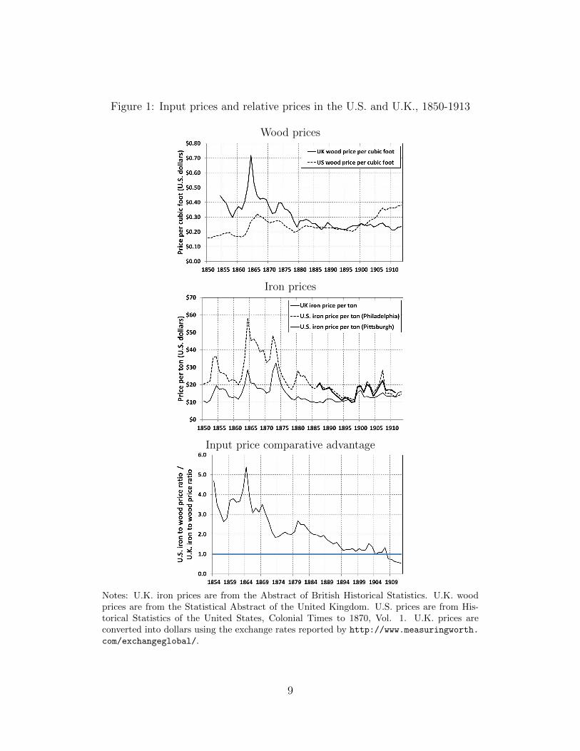
Figure 1: Input prices and relative prices in the U.S. and U.K., 1850-1913

Wood prices

Iron prices

Input price comparative advantage

Notes: U.K. iron prices are from the Abstract of British Historical Statistics. U.K. woodprices are from the Statistical Abstract of the United Kingdom. U.S. prices are from His-torical Statistics of the United States, Colonial Times to 1870, Vol. 1. U.K. prices areconverted into dollars using the exchange rates reported by http://www.measuringworth.

com/exchangeglobal/.

9

shipyards both above and below the locks, naturally substantially increased the cost

of moving vessels into the Great Lakes. The Annual Report to the Commissioners

of the Navy (p. 15) says of this method, “The experiment of building large vessels,

cutting them in two to pass the locks, and then reuniting the parts has been made

successfully in a few instances, but at the present time it does not appear that this

method...will become general.” The report goes on to state that, “Construction on

the seaboard and on the lakes up to the present time should be considered as different

industries, indirectly related.” The result was a largely isolated Great Lakes market,

naturally protected from international competition.

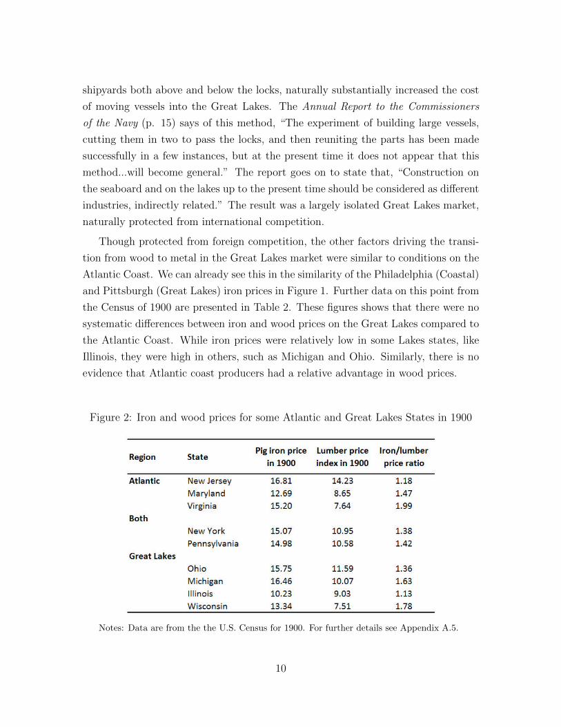
Though protected from foreign competition, the other factors driving the transi-

tion from wood to metal in the Great Lakes market were similar to conditions on the

Atlantic Coast. We can already see this in the similarity of the Philadelphia (Coastal)

and Pittsburgh (Great Lakes) iron prices in Figure 1. Further data on this point from

the Census of 1900 are presented in Table 2. These figures shows that there were no

systematic differences between iron and wood prices on the Great Lakes compared to

the Atlantic Coast. While iron prices were relatively low in some Lakes states, like

Illinois, they were high in others, such as Michigan and Ohio. Similarly, there is no

evidence that Atlantic coast producers had a relative advantage in wood prices.

Figure 2: Iron and wood prices for some Atlantic and Great Lakes States in 1900

Notes: Data are from the the U.S. Census for 1900. For further details see Appendix A.5.

10

On the demand side, incentives for producing metal rather than wood ships in

the Lakes were also similar to on the coast. For example, the transition from sail to

steamships that took place in the Lakes was similar to the transition in the Atlantic

market as a whole, as described in Appendix A.2. The incentives for using metal

provided by opportunities to construct larger ships were weaker in the Great Lakes

than on the Coast, because, as shown in Appendix A.3, maximum ship sizes in the

lakes remained smaller than in the Atlantic.20 On the other hand, metal ships did last

longer on the Lakes because freshwater was less corrosive, which may have provided

some increased incentive for metal ship production there. While ships on the Lakes

did have different designs than those on the coast, such as being longer and skinnier

to maximize use of the available locks, there doesn’t seem to have been any important

differences in the techniques used to construct lake ships.21 Thus, the Great Lakes

market provides us with a benchmark for tracking the development of North Amer-

ican shipbuilding in the absence of foreign competition, while a comparison of the

North American Atlantic Coast and Great Lakes shipbuilding industries provides an

opportunity for assessing the impact of foreign competition on industry development.

Industrial policy and protection from foreign competition played an important role

in the shipbuilding industry. Major shipbuilding nations used a variety of tools to help

protect and nurture domestic shipbuilders. The U.S. was particularly active in this

regard. One tool used by the U.S. was a ban on the use of foreign-built ships for direct

trade between American ports (coastal trade). This policy, which existed throughout

the study period, created a protected market for U.S. shipbuilders, though the size of

this market was limited.22 A second important channel of government influence on

shipbuilding was through the Navy. Both the U.S. and Britain operated government

shipyards and purchased warships exclusively from domestic shipbuilders. Warship

20The smaller size of ships on the Great Lakes was due to the limitations imposed by locks andcanals, particularly the lock between Lake Superior and the lower Great Lakes, as well as depthlimitations in some lake harbors.

21One sign of the similarity of techniques used on the Lakes and the Coast is provided by theAnnual Report of the Commissioners of the Navy from 1901, which suggests that coastal shipbuildersmay be able to learn from the more successful yards on the Great Lakes (p. 15): “...throughthe training of shipbuilders, the invention and improvement of shipbuilding tools, machinery, andmaterials, and through experience gained in the financial and industrial organization of shipyards,the establishments on the Great Lakes are promoting the chance for seaboard growth.”

22Another type of industrial policy, which was applied by nearly all of the major shipbuildingnations, was the subsidization of mail-carrying routes, which had to be served with domestically-built ships. However, these policies only affected a small fraction of shipping tonnage.

11

construction played an important role in the development of the domestic shipbuilding

industry because the demand for Naval vessels gave yards experience and generate

pools of skilled workers. The U.S. began a substantial expansion of the Navy in the

late 1880s and 1890s often described as the “New Navy” because the new ships were

metal rather than wood.23

This study takes advantage of an exogenous source of variation in access to gov-

ernment protection provided by the empirical setting. Specifically, while the U.S.

had access to the full range of protective policies, Canada, as part of the British Em-

pire, did not have the ability to enact similar policies. Specifically, Canada could not

close coastal trade to British-built ships, nor did it have an independent navy during

this period to provide orders to domestic yards or to operate government shipyards.24

Figures presented in Appendix A.7 attest to the importance of this difference. In par-

ticular, while 7.6% of tonnage homeported on the Atlantic Coast of the U.S. in 1912

was constructed in the U.K., on the Canadian Atlantic Coast, vessels constructed in

the U.K. accounted for 46% of total tonnage. Thus, comparing the experience of the

U.S. and Canada allows us to observe the evolution of this industry with and without

access to government protection.

3 Data

This study draws on a unique new data set derived from individual ship listings

on two registers, one produced by Lloyd’s and the other by the American Bureau

of Shipping (ABS, sometimes called “American Lloyd’s”). The primary purpose of

these registers was to provide insurers and merchants with a rating of the quality of

23The importance of Naval shipbuilding is highlighted by Hutchins (1948), who writes that (p.35), “it is probable that a substantial modern shipbuilding industry would have been long in comingin the United States but for the naval expansion of the ’eighties, ’nineties, and early twentiethcentury.” Appendix A.6 describes the increases in U.S. Navy shipbuilding during the study period.

24Canada’s status as part of the British Dominion made enacting protection against the mothercountry “scarcely thinkable” (Sager & Panting, 1990, p. 171). Canada did have the ability to levytariffs against British imports, but without being able to close ports to foreign-built ships, tariffson ships are ineffective at providing protection. There were also practical difficulties. Sager &Panting (1990) explain that because Canada used the British registration system for vessels, it was“virtually impossible to distinguish between British and Canadian ships, and hence a customs dutyon British ships [in the Canadian foreign trade] would be impossible to enforce.” In addition, theRoyal Canadian Navy was not founded until 1910 and initially it was equipped with vessels fromthe Royal Navy, so this avenue of support was unavailable.

12

each ship that they might be asked to underwrite or to ship their products. This

provided shipowners with a strong incentive to have their ship included on at least

one major register, and often more than one. As a result, the registration societies

claimed that the vast majority of major merchant ships (e.g., over 100 tons) were

included on one of the lists.25 This data cover only merchant ships; warships are

not included in the analysis. The vast majority of these were cargo carriers, though

the data also include passenger liners, some fishing and whaling vessels, and other

miscellaneous types (tugs, large barges, etc.).

The registers were published annually and included, for each ship, information on

the location and year of construction, often the shipbuilder, the tonnage, construction

material, and other characteristics of the ship.26 Figure 3 provides an example of the

data from the first page of the Lloyd’s Register for 1871-72. We can see that the first

ship on this list, the A.D. Gilbert, was a schooner (Sr) of 177 tons built in Truro

(UK) by the Hodge shipyard in 1865. The details below the name indicate that this

was a wood ship. The third entry, the A. Lopez, was a screw steamer (ScwStr) and

below the name we can see that this ship was made of iron.27 For cost reasons, I have

digitized only a subset of the information shown in the register in Figure 3: the ship

name, type and construction details (shown in the “Ships” column), the tonnage, and

information on the location of construction, shipyard, and year of launch (shown in

the “Build” column).

This study uses data from registers for three years, 1871, 1889 and 1912.28 Because

the registers include all active ships in these years, and because ships generally last

many years after construction, these snapshots provide coverage for most ships built

between 1850 and the First World War. Specifically, I use the 1871 register to track

ships built between 1850 and 1870, the 1889 register to track ships built between 1871

and 1887, and the 1912 register to track ships from 1888-1911.29 For each snapshot

25To be included on a register, a ship had to be inspected. This often occurred multiple timesduring the construction process and at periodic intervals after construction was complete. To com-plete these inspections, the registration societies employed a set of local inspectors in the majorsshipbuilding areas of the world.

26The register also included additional information about the current owner, home port and masterof each ship. These data were not entered for cost reasons.

27I am grateful to Hathi Trust and the Mystic Seaport Library for providing these scans.28The use of these snapshots is driven primarily by cost concerns. Digitizing each register requires

entering data from thousands of pages of documents by hand, so even with outsourcing this tolow-cost providers the cost is substantial.

29The registers often did not have complete coverage for ships in the year in which they were

13

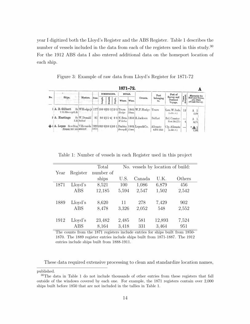
year I digitized both the Lloyd’s Register and the ABS Register. Table 1 describes the

number of vessels included in the data from each of the registers used in this study.30

For the 1912 ABS data I also entered additional data on the homeport location of

each ship.

Figure 3: Example of raw data from Lloyd’s Register for 1871-72

Table 1: Number of vessels in each Register used in this project

Total No. vessels by location of build:Year Register number of

ships U.S. Canada U.K. Others1871 Lloyd’s 8,521 100 1,086 6,879 456

ABS 12,185 5,594 2,547 1,502 2,542

1889 Lloyd’s 8,620 11 278 7,429 902ABS 8,478 3,326 2,052 548 2,552

1912 Lloyd’s 23,482 2,485 581 12,893 7,524ABS 8,164 3,418 331 3,464 951

The counts from the 1871 registers include entries for ships built from 1850-1870. The 1889 register entries include ships built from 1871-1887. The 1912entries include ships built from 1888-1911.

These data required extensive processing to clean and standardize location names,

published.30The data in Table 1 do not include thousands of other entries from these registers that fall

outside of the windows covered by each one. For example, the 1871 registers contain over 2,000ships built before 1850 that are not included in the tallies in Table 1.

14

eliminate duplicate entries that appeared in both registers, identify the construction

material for each ship, etc.31 The analysis in this paper uses only data from the U.K.

as well as the East Coast and Great Lakes regions of the U.S. and Canada.32 Within

these analysis areas, it is possible to identify the exact location of construction for

the vast majority of ships.33

In addition to the main data, I have also collected information on local iron and

lumber prices that will be used as controls in the analysis. These data come from the

U.S. Census of 1900 and are available at the state level. Further details on these data

are available in Appendix A.5.

4 Analysis

This section begins with a review of the key patterns in the data, followed by the

econometric analysis. A useful starting point is Figure 4, which describes the evolution

of ship production in the U.S., U.K., and Canada across the study period using data

from the ship registers. The top panel of Figure 4 shows that the U.S. was the leading

shipbuilder in 1850, with Canada and the U.K. not far behind. However, by 1911

the U.K. was by far the dominant producer. While the U.K. gained a small lead in

the late 1850s and 1860s (due in part to the U.S. Civil War), the main divergence

occurred in the 1880s. We can also see that the U.S. experienced some recovery in the

late 1890s, which corresponded to the reduction in Britain’s advantage in iron prices.

However, despite this reversal the U.S. remained far behind Britain in overall ship

production in 1911. In Canada, where output was comparable to U.S. production

from the 1860s to the 1880s, no similar recovery took place so that it had ceased to

31In the 1912 data I identified 5,538 U.S., British or Canadian ships that were listed in bothregisters. In the 1889 data there are 2,663 duplicates. In the 1871 data, I find 602 ships that werelisted in both.

32The U.K. includes all of Ireland for the purposes of this study. There was very little shipconstruction in the Gulf of Mexico. Construction on the Pacific Coast was also relatively smallduring most of the study period. Pacific shipbuilding, which was heavily concentrated in wood, didgrow late in the study period.

33For ships built in the U.S. and Canada, I am able to identify the construction location for over99% of ship tonnage in data from the 1912 register, over 96% of tonnage in the 1889 registers. Indata from the 1871 registers, the share of tonnage linked to a location within the U.S. and Canada,respectively, is 97.1% and 88.3%. The larger share of tonnage with missing locations in the Canadiandata is due to the fact that only the province of construction was provided for many Canadian shipsregistered in the 1871 Lloyd’s.

15

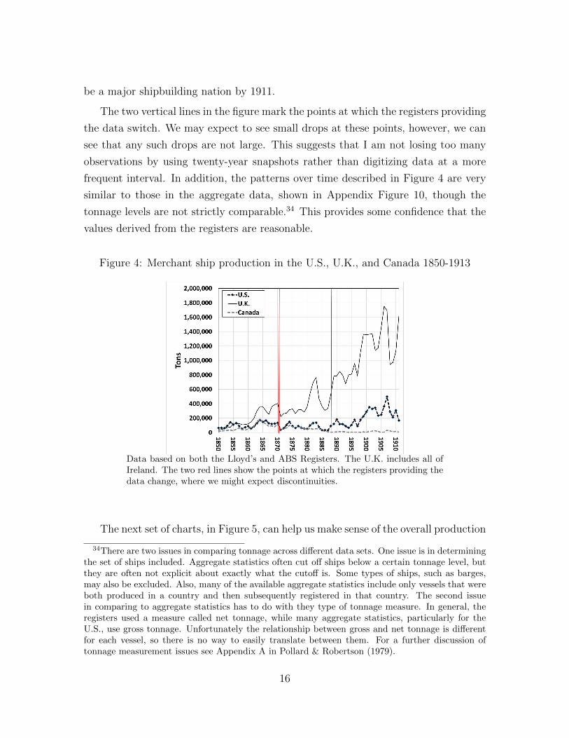
be a major shipbuilding nation by 1911.

The two vertical lines in the figure mark the points at which the registers providing

the data switch. We may expect to see small drops at these points, however, we can

see that any such drops are not large. This suggests that I am not losing too many

observations by using twenty-year snapshots rather than digitizing data at a more

frequent interval. In addition, the patterns over time described in Figure 4 are very

similar to those in the aggregate data, shown in Appendix Figure 10, though the

tonnage levels are not strictly comparable.34 This provides some confidence that the

values derived from the registers are reasonable.

Figure 4: Merchant ship production in the U.S., U.K., and Canada 1850-1913

Data based on both the Lloyd’s and ABS Registers. The U.K. includes all ofIreland. The two red lines show the points at which the registers providing thedata change, where we might expect discontinuities.

The next set of charts, in Figure 5, can help us make sense of the overall production

34There are two issues in comparing tonnage across different data sets. One issue is in determiningthe set of ships included. Aggregate statistics often cut off ships below a certain tonnage level, butthey are often not explicit about exactly what the cutoff is. Some types of ships, such as barges,may also be excluded. Also, many of the available aggregate statistics include only vessels that wereboth produced in a country and then subsequently registered in that country. The second issuein comparing to aggregate statistics has to do with they type of tonnage measure. In general, theregisters used a measure called net tonnage, while many aggregate statistics, particularly for theU.S., use gross tonnage. Unfortunately the relationship between gross and net tonnage is differentfor each vessel, so there is no way to easily translate between them. For a further discussion oftonnage measurement issues see Appendix A in Pollard & Robertson (1979).

16

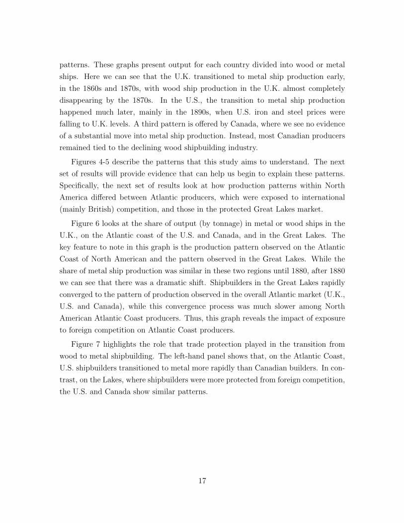
patterns. These graphs present output for each country divided into wood or metal

ships. Here we can see that the U.K. transitioned to metal ship production early,

in the 1860s and 1870s, with wood ship production in the U.K. almost completely

disappearing by the 1870s. In the U.S., the transition to metal ship production

happened much later, mainly in the 1890s, when U.S. iron and steel prices were

falling to U.K. levels. A third pattern is offered by Canada, where we see no evidence

of a substantial move into metal ship production. Instead, most Canadian producers

remained tied to the declining wood shipbuilding industry.

Figures 4-5 describe the patterns that this study aims to understand. The next

set of results will provide evidence that can help us begin to explain these patterns.

Specifically, the next set of results look at how production patterns within North

America differed between Atlantic producers, which were exposed to international

(mainly British) competition, and those in the protected Great Lakes market.

Figure 6 looks at the share of output (by tonnage) in metal or wood ships in the

U.K., on the Atlantic coast of the U.S. and Canada, and in the Great Lakes. The

key feature to note in this graph is the production pattern observed on the Atlantic

Coast of North American and the pattern observed in the Great Lakes. While the

share of metal ship production was similar in these two regions until 1880, after 1880

we can see that there was a dramatic shift. Shipbuilders in the Great Lakes rapidly

converged to the pattern of production observed in the overall Atlantic market (U.K.,

U.S. and Canada), while this convergence process was much slower among North

American Atlantic Coast producers. Thus, this graph reveals the impact of exposure

to foreign competition on Atlantic Coast producers.

Figure 7 highlights the role that trade protection played in the transition from

wood to metal shipbuilding. The left-hand panel shows that, on the Atlantic Coast,

U.S. shipbuilders transitioned to metal more rapidly than Canadian builders. In con-

trast, on the Lakes, where shipbuilders were more protected from foreign competition,

the U.S. and Canada show similar patterns.

17

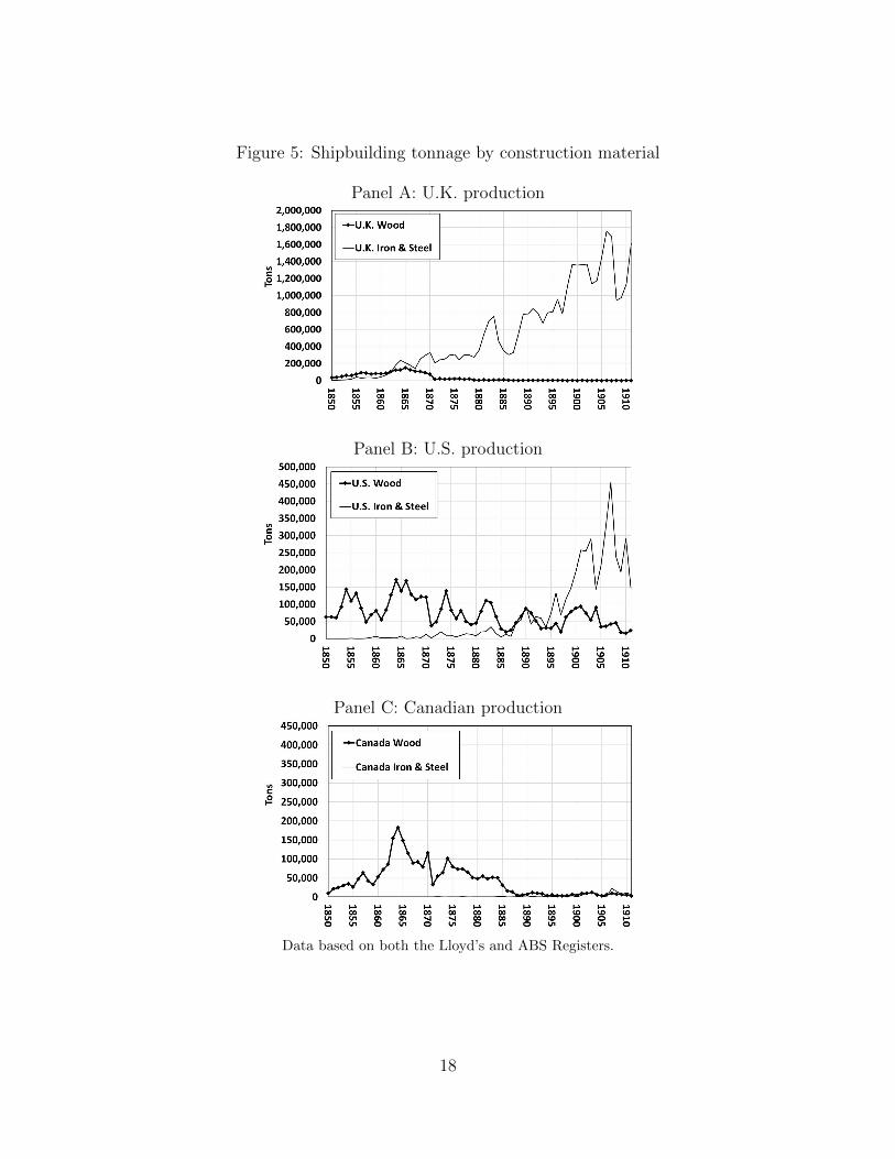
Figure 5: Shipbuilding tonnage by construction material

Panel A: U.K. production

Panel B: U.S. production

Panel C: Canadian production

Data based on both the Lloyd’s and ABS Registers.

18

Figure 6: Evolution of production patterns by region

Data based on both the Lloyd’s and ABS Registers. The U.K. includes Ireland. The “AllAtlantic” category includes production in the U.K., U.S. and Canada.

Figure 7: Evolution of metal share on the Coast vs. the Lakes

Atlantic Coast Great Lakes

Data based on both the Lloyd’s and ABS Registers.

Figure 8 maps the distribution of production of wood and metal ships in the

decades 1871-1880 and 1901-1910. These maps bring us closer to the approach used in

the econometric analysis, which studies patterns at the level of individual shipbuilding

locations. I consider these two periods because the first falls after the U.S. Civil War

but before the elimination of the differences in input prices between the U.S. and

Britain, while the second period falls after the input price differences had disappeared.

These maps illustrate the strong shift in North American ship production from the

Atlantic Coast to the Great Lakes, and the shift from wood to metal ships. It is clear

19

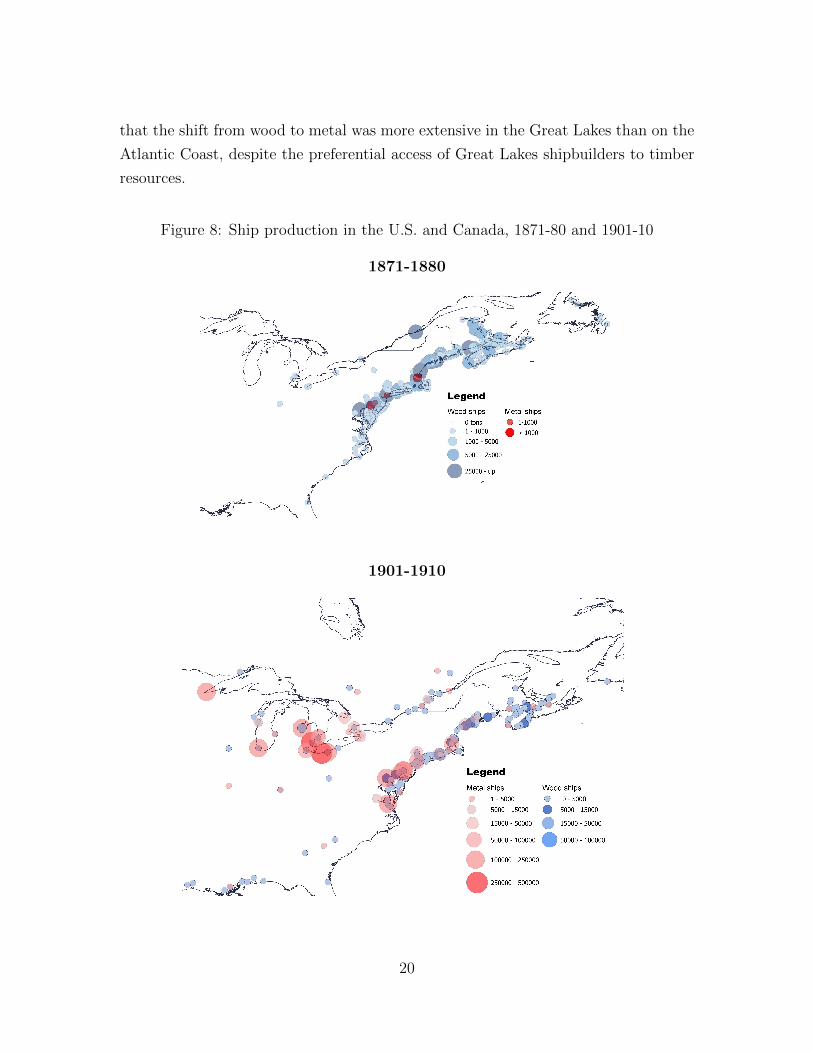
that the shift from wood to metal was more extensive in the Great Lakes than on the

Atlantic Coast, despite the preferential access of Great Lakes shipbuilders to timber

resources.

Figure 8: Ship production in the U.S. and Canada, 1871-80 and 1901-10

1871-1880

1901-1910

20

Figure 8 also shows that on the Atlantic Coast metal ship production was mainly

concentrated in a few locations: Boston, New York, along the Delaware River (Philadel-

phia, Camden, Wilmington, and Chester), Baltimore, and Newport News, Virginia.

Notably, each of these locations was also close to one of the Navy shipyards estab-

lished in the early 19th century, with the exception of Baltimore (where a Coast

Guard shipyard was established in 1899), a point that I will return to in Section 5.

Next, I analyze these patterns econometrically. I begin with a set of regressions

looking at outcomes in the last decade before the First World War. These regressions

are cross-sectional, but in some specifications I include controls for past production

patterns. The first set of results look at whether there are active shipbuilders in a

particular sector and location, using multinomial logit (ML) regressions. The speci-

fication is,

Als = 1[a∗ls > 0] (1)

a∗ls = α1LAKESl + α2USl +XjsΓ + els

where Als is an indicator variable for whether location l is active in shipbuilding sec-

tor s ∈ {wood,metal, both} in the 1901-1910 decade, with inactive as the reference

category, and a∗ls is an unobserved latent variable which depends on the set of ex-

planatory variables. LAKESl is an indicator variable for whether the location is in

the Great Lakes region while USl is an indicator for whether the location is in the

U.S. The error term els follows a logistic distribution.

Among the control variables that I consider is whether a location has been active

in shipbuilding in some past decade (typically 1871-80, which avoids the decade of

the U.S. Civil War but predates the input price convergence) at all, or in sector

s specifically, and if so, the tonnage produced in that past decade in the location

overall or in sector s specifically. In some specifications I also control for production

patterns in other nearby locations. These controls are meant to help capture both the

location’s physical assets for ship production, such as a deep harbor or easier access

to inputs.

A natural concern in this analysis is that errors may be spatially correlated. As one

approach to dealing with this concern, I have generated results clustering standard

21

errors by U.S. state or Canadian province for all of the main specifications. In general

this results in a slight reduction in the size of the estimated standard errors, suggesting

weak negative spatial correlation across shipbuilding locations. To be conservative, I

report robust standard errors in the main results tables.

Table 2 presents ML regression results based on Eq. 1. These regressions are

run on the full set of U.S. and Canadian shipbuilding locations on the East Coast

or Great Lakes which were active at some point in the 1850-1910 period. To keep

the table manageable I do not report coefficient estimates for the control variables in

Table 1. The full results can be found in Appendix A.8.

Column 1 presents results without any additional controls. In Column 2, I add

in indicators for whether the location was active in shipbuilding in the 1870s, wither

the location was active in sector s specifically in the 1870s, tonnage produced in

the location in the 1870s, and tonnage produced in the location in sector s in the

1870s. In Column 3 I also include controls for production of ships in each sector in

other locations within 100km in the 1870s. The results in Columns 1-3 suggest that

locations in the Great Lakes were more likely to be active in the production of metal

ships, either alone or in combination with wood shipbuilding, relative to exiting the

market. Locations in the U.S. were also more likely to be active in metal shipbuilding

in combination with wood, relative to exiting the market. At the bottom of the

table I include additional tests comparing the probability of being active in metal

shipbuilding or in both sectors to the probability of being active in wood shipbuilding

alone. In general the effect of the Great Lakes on whether a location is active in metal

is statistically different from the impact of the Great Lakes on activity in wood only.

Column 4 includes additional controls for the iron and lumber price at the state

level, together with controls for whether the location was active in the 1870s and the

tonnage produced in the location in the 1870s. Note that the controls for iron and

lumber prices are available for only a subset of U.S. states, so the sample size drops

substantially and we cannot compare the impact of being in the U.S. vs. Canada.

Column 5 includes all the controls from Column 4 together with additional controls

for production in locations within 100km in the 1870s. While the smaller sample size

means the results in Columns 4-5 are not as clear as those in Columns 1-3, I still tend

to find evidence that locations in the Great Lakes were more likely to be active in

metal shipbuilding.

22

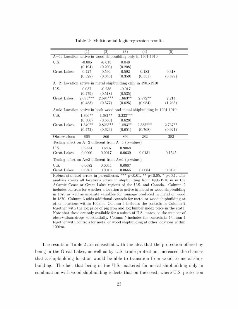
Table 2: Multinomial logit regression results

(1) (2) (3) (4) (5)A=1: Location active in wood shipbuilding only in 1901-1910

U.S. -0.005 -0.015 0.048(0.194) (0.203) (0.208)

Great Lakes 0.427 0.594 0.592 0.182 0.318(0.328) (0.346) (0.359) (0.551) (0.599)

A=2: Location active in metal shipbuilding only in 1901-1910

U.S. 0.037 -0.238 -0.017(0.479) (0.518) (0.535)

Great Lakes 2.685*** 2.594*** 1.863** 2.872** 2.214(0.483) (0.577) (0.625) (0.984) (1.235)

A=3: Location active in both wood and metal shipbuilding in 1901-1910

U.S. 1.396** 1.681** 2.233***(0.506) (0.580) (0.628)

Great Lakes 1.549** 2.826*** 1.893** 2.535*** 2.737**(0.472) (0.623) (0.651) (0.768) (0.921)

Observations 866 866 866 282 282

Testing effect on A=2 different from A=1 (p-values)

U.S. 0.9334 0.6807 0.9068Great Lakes 0.0000 0.0017 0.0639 0.0131 0.1545

Testing effect on A=3 different from A=1 (p-values)

U.S. 0.0082 0.0044 0.0007Great Lakes 0.0361 0.0010 0.0666 0.0084 0.0195

Robust standard errors in parentheses. *** p<0.01, ** p<0.05, * p<0.1. Theanalysis covers all locations active in shipbuilding from 1850-1910 in in theAtlantic Coast or Great Lakes regions of the U.S. and Canada. Column 2includes controls for whether a location is active in metal or wood shipbuildingin 1870 as well as separate variables for tonnage produced in metal or woodin 1870. Column 3 adds additional controls for metal or wood shipbuilding atother locations within 100km. Column 4 includes the controls in Column 2together with the log price of pig iron and log lumber index price in the state.Note that these are only available for a subset of U.S. states, so the number ofobservations drops substantially. Column 5 includes the controls in Column 4together with controls for metal or wood shipbuilding at other locations within100km.

The results in Table 2 are consistent with the idea that the protection offered by

being in the Great Lakes, as well as by U.S. trade protection, increased the chances

that a shipbuilding location would be able to transition from wood to metal ship-

building. The fact that being in the U.S. mattered for metal shipbuilding only in

combination with wood shipbuilding reflects that on the coast, where U.S. protection

23

mattered, most shipbuilding locations had a history of wood ship production and re-

mained active in that sector even after they also began producing metal ships. Only

in the Great Lakes did many new shipyards open in locations without a history of

wood ship production, and there the impact of U.S. protection from competition was

much less important.

Another set of results in Appendix A.8 considers both the ship’s construction

material and power source (sail vs. steam). These results show that Great Lakes

producers were more likely to be active in both metal sailing ship and metal steamship

production. This shows that differences in metal ship production between the lakes

and the coast were not driven by differences in demand for sailing vs. steamships.

There is also some slightly weaker evidence that U.S. producers were more likely

than Canadian producers to be active in both steamship production and metal ship

production.

Next, I consider an alternative regression approach which looks at the shipbuilding

tonnage produced in a location in 1900-1910 conditional on the location being active

in a particular sector in that decade. The regression specification is,

ln(Yls) = β0METALs + β1LAKESl + β3USl (2)

+ β4(METALs × LAKESl) + β5(METALs × USl) +XjsΓ + εjs

where Yls is ship tonnage of type s produced in location l, METALs is an indicator

for the metal ship sector, and the remaining variables are defined as before. The

main coefficients of interest in this regression are β4 and β5 which reflect the impact

of being in the Great Lakes market or in the U.S., respectively, on metal ship output

relative to wood.

Table 3 presents the results of regressions based on Eq. 2. Column 1 presents

baseline results while Column 2 adds in controls for whether a location was active in

shipbuilding in the 1870s, whether it was active in sector s in the 1870s, tonnage in

the sector in the 1870s, and overall tonnage produced in the location in the 1870s.35

Column 3 adds additional controls for activity and tonnage in other locations within

35I include tonnage as a control rather than log tonnage so as not to drop locations where noproduction took place in the 1870s.

24

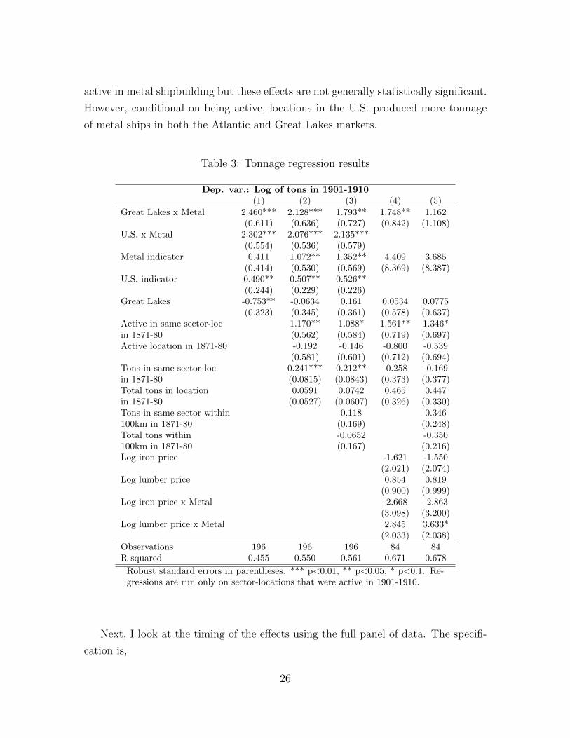
100km in the 1870s. In all of the results in Column 1-3 we observe evidence that

locations in the Great Lakes or in the U.S. that were active also produced more

tonnage in metal shipbuilding. The control variables indicate that U.S. shipyards

tended to be larger overall, and that sector-locations that were active and produced

more tonnage in the 1870s continued to produce more tonnage in the 1901-1910

period. However, being active in the other sector, or producing more tonnage in the

other sector, was not associated with more output in 1901-1910.

Finally, Columns 4-5 add in controls for the state iron and lumber prices. Note

that this substantially reduces the sample size and makes it impossible to compare

locations in the U.S. and Canada. Still, even with the reduced sample size we observe

some evidence that locations in the Great Lakes produced more iron ship tonnage

conditional on being active, though this finding is not statistically significant in Col-

umn 5. It is also worth noting that the coefficient estimates indicate that locations

with lower iron prices and higher lumber prices produced more metal ship tonnage,

as we would expect, though these results are not statistically significant.

The results in Table 3 suggest that, conditional on a location being active in a

particular sector, tonnage of metal ship production was higher in locations in the

Great Lakes region and those in the U.S. The magnitudes of these effects are large;

either being in the Great Lakes or in the U.S. is associated with an increase in metal

ship production of around 1-2 log points.36 Additional results, in Appendix A.9 show

that these patterns are being driven entirely by steamships. Moreover, the impact of

the Great Lakes and the U.S. markets continues to hold when we look only within

steamships, so these effects are not being driven by a different mix of steamships vs.

sailing ships in different markets.

It is interesting to consider whether results similar to those shown in Tables 2-3

are obtained if we look at the impact of being in the Great Lakes within only the

U.S. or only Canada, or the impact of being in the U.S. in only the Lakes or only

the Atlantic. This is explored in Appendix A.10. I find that locations in the Great

Lakes are more likely to be active in metal shipbuilding in 1901-1910 in both the

U.S. and Canada. Conditional on being active, locations in the Great Lakes also

produce more metal ship tonnage. Focusing separately on either the Atlantic Coast

or Great Lakes, I find weak evidence that locations in the U.S. were more likely to be

36Mean production in active metal shipbuilding locations in the data in 1901-10 was 66,000 tons.

25

active in metal shipbuilding but these effects are not generally statistically significant.

However, conditional on being active, locations in the U.S. produced more tonnage

of metal ships in both the Atlantic and Great Lakes markets.

Table 3: Tonnage regression results

Dep. var.: Log of tons in 1901-1910(1) (2) (3) (4) (5)

Great Lakes x Metal 2.460*** 2.128*** 1.793** 1.748** 1.162(0.611) (0.636) (0.727) (0.842) (1.108)

U.S. x Metal 2.302*** 2.076*** 2.135***(0.554) (0.536) (0.579)

Metal indicator 0.411 1.072** 1.352** 4.409 3.685(0.414) (0.530) (0.569) (8.369) (8.387)

U.S. indicator 0.490** 0.507** 0.526**(0.244) (0.229) (0.226)

Great Lakes -0.753** -0.0634 0.161 0.0534 0.0775(0.323) (0.345) (0.361) (0.578) (0.637)

Active in same sector-loc 1.170** 1.088* 1.561** 1.346*in 1871-80 (0.562) (0.584) (0.719) (0.697)Active location in 1871-80 -0.192 -0.146 -0.800 -0.539

(0.581) (0.601) (0.712) (0.694)Tons in same sector-loc 0.241*** 0.212** -0.258 -0.169in 1871-80 (0.0815) (0.0843) (0.373) (0.377)Total tons in location 0.0591 0.0742 0.465 0.447in 1871-80 (0.0527) (0.0607) (0.326) (0.330)Tons in same sector within 0.118 0.346100km in 1871-80 (0.169) (0.248)Total tons within -0.0652 -0.350100km in 1871-80 (0.167) (0.216)Log iron price -1.621 -1.550

(2.021) (2.074)Log lumber price 0.854 0.819

(0.900) (0.999)Log iron price x Metal -2.668 -2.863

(3.098) (3.200)Log lumber price x Metal 2.845 3.633*

(2.033) (2.038)Observations 196 196 196 84 84R-squared 0.455 0.550 0.561 0.671 0.678

Robust standard errors in parentheses. *** p<0.01, ** p<0.05, * p<0.1. Re-gressions are run only on sector-locations that were active in 1901-1910.

Next, I look at the timing of the effects using the full panel of data. The specifi-

cation is,

26

Ylst =∑t

β0t(METALs ×Dt) +∑t

β1t(LAKESl ×METALs ×Dt)

+∑t

β2t(LAKESl ×WOODs ×Dt) +∑t

β3t(USl ×METALS ×Dt) (3)

+∑t

β4t(USl ×METALS ×Dt) +XjstΓ +∑t

ηtDt + φls + εjs

where Ylst is ship tonnage, WOODs is an indicator variable for the wood shipbuilding

sector, Dt is a set of indicator variables for each decade, and φls is a set of fixed effects

for each sector-location. These regressions allow me to look at the impact of being

in the Great Lakes or in the U.S. on iron ship output while controlling for changes

in output over time as well as differences in regional production patterns over time.

Because we may be concerned about serial correlation in these regressions, standard

errors are clustered by sector-location. I focus on tonnage rather than log tons in this

specification to avoid dropping observations for locations that were inactive (produced

zero tons) in at least some decades.

The coefficients of interest in Eq. 3 are the vectors β1t - β4t, which reflect the

impact of being in the Great Lakes or being in the U.S. in each decade within each

ship type. These parameter estimates, together with their 95% confidence intervals,

are described in Figure 9. The top panel shows the coefficients estimated for each

decade on the interaction between the Great Lakes and either metal or wood ship-

building. These results suggest that being located in the Great Lakes was, if anything,

associated with lower production tonnage prior to the 1880s. Then, starting in the

1890s, there was a relative increase in tonnage produced on the Great Lakes which

was concentrated in metal shipbuilding. This timing corresponds with the fall in U.S.

iron and steel prices as well as an increase in demand for Great Lakes shipping.

In the bottom panel, we see that the U.S. had an advantage in ship production

relative to Canada in the 1850s but this fell during the decade of the U.S. Civil

War. This was followed by a relative recovery beginning in the 1880s which initially

occurred in both wood and metal shipbuilding. However, starting in the 1890s we can

see that wood and metal shipbuilding diverged, with metal shipbuilding experiencing

a relative increase in the U.S. compared to Canada. This timing corresponds with

the fall in metal prices as well as the expansion of the U.S. Navy.

27

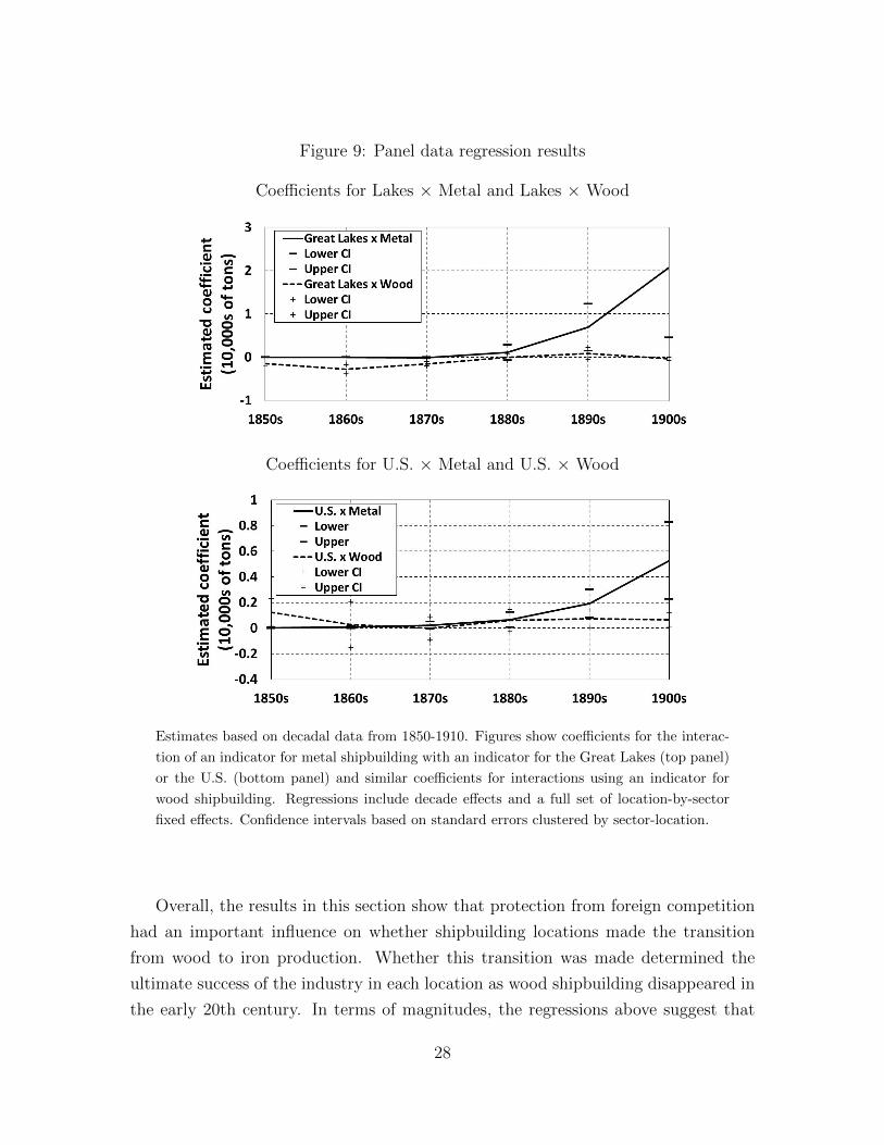
Figure 9: Panel data regression results

Coefficients for Lakes × Metal and Lakes × Wood

Coefficients for U.S. × Metal and U.S. × Wood

Estimates based on decadal data from 1850-1910. Figures show coefficients for the interac-

tion of an indicator for metal shipbuilding with an indicator for the Great Lakes (top panel)

or the U.S. (bottom panel) and similar coefficients for interactions using an indicator for

wood shipbuilding. Regressions include decade effects and a full set of location-by-sector

fixed effects. Confidence intervals based on standard errors clustered by sector-location.

Overall, the results in this section show that protection from foreign competition

had an important influence on whether shipbuilding locations made the transition

from wood to iron production. Whether this transition was made determined the

ultimate success of the industry in each location as wood shipbuilding disappeared in

the early 20th century. In terms of magnitudes, the regressions above suggest that

28

the advantages of being in the U.S. were nearly as large as the benefits of being in the

isolated Great Lakes market in terms of shipbuilder’s ability to transition to metal

ship production.

5 Evidence of learning

A number of previous studies provide evidence for the important role played by learn-

ing in the shipbuilding industry. The most influential paper in this vein, Thompson

(2001), examines the impact of cumulative output on productivity for ships sharing

a common design within a given set of yards, while controlling for factors such as

physical capital within each yard. Using this controlled setting, Thompson provides

evidence that cumulative production improved shipbuilding efficiency. Specifically,

his estimates suggest that the elasticity of output with respect to cumulative experi-

ence was around 0.21-0.26, while controlling for capital and labor inputs.37

Replicating Thompson’s very detailed approach is infeasible in the setting that I

consider, which spans hundreds of yards and thousands of different ship designs over

many decades. However, it is possible to provide some suggestive evidence on the

role played by local learning in the setting that I consider. In this section I provide

two types of evidence on learning effects.

The first piece of evidence on learning comes from a set of regressions looking at

the relationship between output and cumulative previous production. This exercise is

in the spirit of previous work in this area, but importantly, I am not able to control for

inputs in these regressions. This raises the concern that cumulative output may just

be capturing the impact of factors such as installed shipbuilding capacity. To help

address this issue, and to highlight the localized nature of learning, I consider both the

impact of cumulative production within a location as well as the additional influence

of cumulative production in nearby areas. However, while looking at effects across

nearby locations can help me avoid conflating the effects of learning from factors

such as fixed capital investments, there is still a concern that this relationship may

reflect fixed local advantages in a particular shipbuilding sector. Thus, it is important

37The lower elasticity is derived from regression in which cumulative experience is based on laborhours while the higher value comes from regressions using cumulative output in place of labor hours.An earlier study, Argote et al. (1990) estimated a larger effect of cumulative experience, around0.44, using a cruder control for capital inputs.

29

to recognize that these are merely exploratory regressions and not cleanly identified

causal effects.

Next, I attempt to provide some better-identified causal evidence of learning ef-

fects. To do so, I focus on the impact of proximity to U.S. Naval Shipyards. Proximity

to Naval shipyards could benefit private-sector shipyards by producing pools of skilled

workers or through technology spillovers. Also, proximity improved access to Navy

contracts, which could have had beneficial learning effects that spilled over into the

construction of merchant ships.38 A key feature of the Navy shipyards in operation

during the period that I study is that their locations were all determined around

1800, well before the introduction of metal ships.39 Thus, while Naval shipyards were

situated in locations with advantages for shipbuilding overall, the key identification

assumption in this analysis relies on the fact that these locations were not chosen

because of specific advantages in metal, relative to wood, shipbuilding.

Results examining the relationship between output in 1901-1910 and cumulative

previous production (since 1850) are shown in Table 4. Columns 1-2 present results

looking at how cumulative production within a location prior to 1901 was related to

output in the location in 1901-1910. We can see that, in both the wood and metal sec-

tors, previous cumulative production in the same sector-location is related to current

production with an elasticity of around 0.2. Also, the third row of estimated coeffi-

cients shows that after accounting for cumulative production in the sector-location,

there is no evidence that cumulative production in the location overall was associated

with greater output. Thus, there is no evidence that experience obtained in one sector

spilled over into the other.

38Indeed, using a list of firms that receive Navy contracts from Smith & Brown (1948), I findevidence that U.S. coastal shipyards that were within 50km of Navy shipyards were more likelyto obtain Navy contacts. Also, locations that obtained a Navy contract at some point between1885 and 1912 produced more metal merchant ship tonnage. Including controls for Navy contractsreduces the estimated impact of proximity to Navy shipyards on metal merchant ship tonnage, butproximity continues to have a statistically significant positive impact even when these controls areincluded.

39The five Naval shipyards in operation during the period I study were in Portsmouth, VA (NorfolkNSY, opened 1767), Boston, MA (opened 1800), New York City (Brooklyn NSY, opened 1800),Philadelphia (opened 1801), and Kittery, ME (opened 1800). The only other early Atlantic shipyard,in Washington, DC, was opened 1799 but this yard largely ceased ship construction after the War of1812 because the Anacostia River was too shallow to accommodate larger vessels. A Coast Guardshipyard was opened in Baltimore in 1899, but I do not include that in my analysis because it islikely that the location of that yard was influenced by Baltimore’s potential as an iron and steelshipbuilding center.

30

In Columns 3-4 I add in additional variables reflecting cumulative production in

other nearby (within 50km) locations. These provide evidence that cumulative pro-

duction in nearby locations was associated with increased output in metal shipbuilding

but not in wood shipbuilding. It is not clear why we observe the difference between

metal and wood shipbuilding here. One potential reason may be that, because wood

was a long-established sector, knowledge had fully diffused so local learning no longer

mattered. In Column 5 I look at the additional impact of cumulative production in

locations from 50-100km away. Here I observe no evidence of an additional impact,

which suggests that any learning effects in metal shipbuilding were quite localized.

Finally, note that accounting for these local learning effects has little impact on the

own-location coefficients.

Table 4: Cumulative production results

DV: Log tons produced in a sector-location(1) (2) (3) (4) (5)

Log cumulative tons 0.203*** 0.190*** 0.197*** 0.185*** 0.185***by 1900 x Metal (0.0559) (0.0565) (0.0554) (0.0564) (0.0564)

Log cumulative tons 0.203*** 0.178*** 0.232*** 0.217*** 0.217***by 1900 x Wood (0.0617) (0.0677) (0.0566) (0.0625) (0.0613)

Total log cum. tons 0.0249 0.0463 0.000890 0.0160 0.0163in location by 1900 (0.0581) (0.0642) (0.0520) (0.0585) (0.0573)

Log cum. tons within 0.120*** 0.108** 0.111**50km x Metal (0.0399) (0.0442) (0.0469)

Log cum. tons within -0.0207 -0.0187 -0.025550km x Wood (0.0280) (0.0280) (0.0413)

Log cum. tons within 0.023950-100km x Metal (0.0499)

Log cum. tons within 0.010850-100km x Wood (0.0413)

Additional controls:Active loc in 1870s Yes Yes YesActive sector-loc in 1870s Yes Yes YesTons in loc. in 1870s Yes Yes YesTons in sector-loc. in 1870s Yes Yes YesObservations 196 196 196 196 196R-squared 0.626 0.637 0.640 0.648 0.649

Robust standard errors in parentheses. *** p<0.01, ** p<0.05, * p<0.1. Regressions arerun only on sector-locations that were active in 1901-1910. All Columns include indicatorvariables for whether the sector is metal, whether the location was in the Great Lakes,whether the location was in the U.S., and the interaction of each of these variables with themetal sector indicator.

31

It is interesting to compare these results to the findings of previous work. It is

striking how similar the magnitude effects of cumulative output within a location on

current output are to estimates from Thompson (2001). Of course, these results are

not strictly comparable because he is able to control for input usage while I am not.

In general, we would expect this to cause his elasticity estimates to be smaller than

mine. However, Thompson is also looking at learning in the repeated production of

the same ship type, while my data includes a very wide variety of types. If cumulative

production has a larger effect within the same type of ship then we should expect

his estimates to be larger than mine. Thus, it is not clear a priori whether to expect

my estimates to be larger or smaller than previous results, but the fact that they are

fairly similar suggests that my results are in the right ballpark.

It is also possible to compare the effect of spillovers across yards shown in Table

4 to results on cross-yard spillovers from Thornton & Thompson (2001). Looking at

productivity in 25 Navy yards during WWII, they find that cross-yard spillovers were

limited. The results in Table 4 suggest that cross-yard effects may be important, but

that these are highly localized. The localized nature of these effects may explain why

Thornton & Thompson (2001) find weak cross-yard spillover effects, since the yards

in their analysis are often far apart. The localized nature of these effects also provides

a clue to the nature of the underlying channels, a topic that I return to later.

Results looking at the impact of proximity to U.S. Navy shipyards are presented

in Table 5. These regressions are run only on U.S. Atlantic Coast shipbuilders using

the log tonnage regression specification from Eq. 2. Columns 1-3 present results

using all U.S. Atlantic coast locations. In Columns 5-6 I drop all locations within

Pennsylvania, New York, New Jersey, and Massachusetts. This helps address concerns

that results may be due to the fact that three of the Naval shipyards were located in

the major cities of Boston, New York and Philadelphia.40 All of the results suggest

that close proximity to a Naval shipyard – within 50km – has a positive impact on

tonnage of metal ships produced. The impact of proximity to naval shipyards on

wood shipbuilding tends to be negative, suggesting that private shipyards near the

Navy yards were more likely to switch from wood to metal ship construction, or that

metal shipbuilding pushed wooden shipbuilding out of these locations.

40The results are also robust to dropping, individually, other major Atlantic Coast shipbuildingstates such as Connecticut, Maine, Maryland or Virginia. Thus, it does not appear that they arebeing driven by any one state.

32

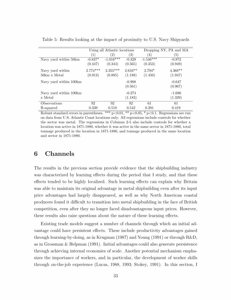
Table 5: Results looking at the impact of proximity to U.S. Navy Shipyards

Using all Atlantic locations Dropping NY, PA and MA(1) (2) (3) (4) (5)

Navy yard within 50km -0.837* -1.016*** -0.329 -1.546*** -0.972(0.447) (0.344) (0.565) (0.353) (0.949)

Navy yard within 2.774*** 2.355*** 2.616** 2.794* 4.368**50km x Metal (0.913) (0.885) (1.188) (1.450) (1.947)

Navy yard within 100km -0.908 -0.647(0.561) (0.967)

Navy yard within 100km -0.274 -1.686x Metal (1.183) (1.329)

Observations 92 92 92 61 61R-squared 0.339 0.518 0.542 0.391 0.419

Robust standard errors in parentheses. *** p<0.01, ** p<0.05, * p<0.1. Regressions are runon data from U.S. Atlantic Coast locations only. All regressions include controls for whetherthe sector was metal. The regressions in Columns 2-5 also include controls for whether alocation was active in 1871-1880, whether it was active in the same sector in 1871-1880, totaltonnage produced in the location in 1871-1880, and tonnage produced in the same locationand sector in 1871-1880.

6 Channels

The results in the previous section provide evidence that the shipbuilding industry

was characterized by learning effects during the period that I study, and that these

effects tended to be highly localized. Such learning effects can explain why Britain

was able to maintain its original advantage in metal shipbuilding even after its input

price advantages had largely disappeared, as well as why North American coastal

producers found it difficult to transition into metal shipbuilding in the face of British

competition, even after they no longer faced disadvantageous input prices. However,

these results also raise questions about the nature of these learning effects.

Existing trade models suggest a number of channels through which an initial ad-

vantage could have persistent effects. These include productivity advantages gained

through learning-by-doing, as in Krugman (1987) and Young (1991) or through R&D,

as in Grossman & Helpman (1991). Initial advantages could also generate persistence

through achieving internal economies of scale. Another potential mechanism empha-

sizes the importance of workers, and in particular, the development of worker skills

through on-the-job experience (Lucas, 1988, 1993; Stokey, 1991). In this section, I

33

conduct a review of available evidence describing the operation of the shipbuilding

industry during this period with the aim of differentiating between these explanations.

To evaluate these channels, we need to establish some stylized facts about the in-

dustry during the study period. One of the most notable features of the international

shipbuilding industry was the high level of competition that existed throughout the

study period, particularly outside of the small number of firms that produced the

largest luxury ocean liners or warships.41 Hutchins (1948), for example, describes

shipbuilding as “naturally one of the most highly competitive of all markets...”42

Consistent with these reports, the HHI calculated from the data used in this study,

for the U.K. only (where I have better data on individual firms), ranges from 173-348

for the years from 1880-1912, indicating a very low level of industry concentration.

Since most of the largest firms in the world were in the U.K., concentration levels

across all world producers are likely to have been even lower. One reason for this

diffuse market structure was the fact that geographic features placed limitations on

the size of individual shipyards.

One implication of the highly competitive and fragmented nature of the shipbuild-

ing industry during this period is that we can rule out internal scale economies as a

primary source of persistent advantages Moreover, internal economies of scale would

not explain the learning spillovers across nearby locations documented in the last

section. Another consequence of the highly competitive nature of the industry was

that shipbuilders had few resources to put into research and development efforts. As

a result, the available evidence suggests that Britain’s initial advantages were unlikely

to have been generated by a lead in R&D.43

Another feature of the industry was that output was largely driven by demand

factors, which were highly volatile over time.44 As a result, shipbuilders largely took

41It is important to distinguish shipbuilding from the shipping industry, where combinationsbetween the major lines substantially reduced competition.

42Pollard & Robertson (1979) states that, “the industry was highly competitive in this trampcargo class, which constituted the majority of its output...”

43For example, Pollard & Robertson (1979) write that (p. 148), “Many improvements, if notmost, however, were developed outside of the industry, in the steel-making, electrical products, orengineering industries...it was only necessary for the shipbuilders to adopt innovations after thebasic research had been done elsewhere. Few laboratories were established in the yards, and as thereluctance to use experimental tanks [to test ship designs] demonstrates, builders were not even veryinterested in investing funds to solve problems peculiar to their industry.”

44Pollard & Robertson (1979) explain that, “freight rates were based on the demand for shippingservices relative to the existing pool of tonnage. As new tonnage was only a small portion of the total

34

prices as given and sought to produce ships at the lowest possible cost. The primary

strategy that shipyards used to cope with volatile demand was to limit, as much as

possible, capital expenditures. As Pollard & Robertson (1979) (p. 28-29) describe,

The principal task of the shipbuilders was to minimize total overhead

expenses while maintaining the ability to build large and complex ships

at prices that were competitive on the world market...The experience

of German and especially American shipbuilders had demonstrated the

dangers of heavy capital expenditures...In the United States, vast over-

heads crippled builders in all but the best years. British yard owners

were able to take advantage of their more highly skilled workforces by

investing only in equipment that was absolutely necessary to manip-

ulate the large, heavy, and hard components of modern ships, and by

refusing to purchase as many labor-saving machines as German and

American builders did.

This quote emphasizes the central role played by skilled workers in the shipbuilding

industry during this period. One important feature of skilled work in the shipbuilding

industry is that a large number of different types of skill work were required. As an

example, the records of the Fairfield Shipbuilding and Engineering Company include

many different groups of skilled workers: angle-iron smiths, fitters, riveters, caulkers,

borers, smiths & strikers, mechanics, carpenters, patternmakers, boatbuilders, join-

ers, cabinetmakers, polishers, coppersmiths, plumbers, tinsmiths, sheet iron workers,

painters, redleaders, cementers, riggers and draftsmen.45 Each group was paid at

different wage rates, used in different phases of the construction process, and in some

cases represented by different unions. Moreover, no single skill made up over 11.5%

of total costs. Additional evidence suggests that, in Britain at least, skilled workers

made up roughly 60% of the total workforce.46 While some of these skills were also

used in wood shipbuilding, or in other engineering industries, many of them were

specialized to metal shipbuilding.

The skills used in the shipyard were gained through experience on the job. This

process can be observed most easily in the case of Britain, where the apprenticeship

amount available, freight rates affected shipbuilding output much more strongly than the converse,although new tonnage did help to drive down rates at the peak of the cycle of freights.”

45See Pollard & Robertson (1979) p. 78.46See Pollard & Robertson (1979) Table 8.1.

35

system was more developed than in North America. For craftsmen in the shipyard,

the apprenticeship period lasted from 5-7 years depending on the trade. Employers

benefited from the low-wage labor provided by apprentices, but also suffered from

the fact that, in Britain at least, indentured apprentices could not be laid off during

downturns.

The quote from Pollard & Robertson above also highlights another important

fact; evidence suggests that American producers were actually equipped with more

advanced technology than their British competitors. For example, American yards

were more likely to adopt more efficient electrical power systems, while British yards

continued to use less efficient steam power.47 The fact that American yards were using

more advanced construction technologies provides further evidence that innovation

was not behind the persistence of British dominance. In fact, Hutchins (1948) found

that (p. 50), “American shipyard work which could be effectively mechanized cost no

more than that in Britain, but handicraft work, of which there was a large amount, was

much more expensive.” Despite using more advanced technology, evidence suggests

that the cost of producing most merchant ship types in U.S. yards was much higher

than in Britain.48 In the end,

expensive equipment could not compensate for the lower level of skills

and more irregular output in Germany and America., especially in

the construction of mercantile tramps. Thus, despite Britain’s inferior

capital equipment, the output per man hour was still highest in Britain

at the end of the [19th] century” (Pollard & Robertson, 1979)[p. 47].

Additional evidence also suggests that the dearth of skilled shipbuilders in the

U.S., and the consequent higher labor costs, was the primary factor in reducing the

competitiveness of U.S. yards. For example, the Report of the Merchant Marine

Commission, ordered by Congress and published in 1905, argues that, in explaining

the relative weakness of the U.S. shipbuilding industry, “The real dominant factor is

thus not the price of materials, but the high wages of the skilled American workmen

47See Pollard & Robertson (1979) Ch. 6. In fact, many shipyard innovations, such as pneumatictools were actually developed in America or Germany and then later slowly adopted in Britain.

48Hutchins (1948), for example, suggests that (p. 47), “British costs were from 30 to 40 percentless.” The Report of the Merchant Marine Commission found that in 1905 the difference was 30 to50 percent (p. viii).

36

who fashion the plates and beams into the finished ship.”49 That report goes on to

offer the following example:

Convincing proof on this point was offered in 1900, when steel plates

and beams, because of labor troubles abroad, were selling at $40.86 in

England, and $28 in the United States. Boston shipowners at that

time invited bids from an American and a British builder for a cargo

steamship of about 5,000 tons capacity. With both yards figuring for a

small competitive profit, the American estimate was $275,000 and the

English $214,000. The material of the American ship would have cost

$63,000; of the English ship, $80,000. But this difference was more

than offset by the higher wages paid to the American shipyard mechan-

ics. However, the narrowing of the difference of shipyard labor cost

that will come with increased experience, improved standardizing and

constant production, as it has come already in the bridge and locomo-

tive works, makes the reduced cost of materials a factor of undeniable

importance.

The last sentence in this quote is notable, because it suggests that the lack of

skilled workers and higher labor costs in iron and steel shipbuilding in the U.S. were

not found in other similar engineering industries.50 Further evidence on the impor-

tance of skilled craft workers is provided by Hutchins (1948), who states, “in 1900

wage costs in American yards were from 50 to 100 per cent above those of Great

Britain...In general, American shipyard work which could be effectively mechanized

cost no more than that in Britain, but handicraft work, of which there was a large

amount, was much more expensive.”

Conditions were similar in Canada. For example, focusing on the Maritime

Provinces, Sager & Panting (1990) write that (p. 12), “The best contemporary es-

timates were that Nova Scotia possessed all the necessary advantages for steel ship-

building except skilled labor.”51

49This report was requested by the President and prepared by a commission consisting of fiveSenators and five Representatives. Their findings were based on a large number of public hearingswhich took place in cities throughout the U.S.

50In fact, evidence from Broadberry & Irwin (2006) suggests that across all manufacturing, workersin the U.S. were more productive than those in the U.K. during the period covered by this study.

51They also describe how, “It is difficult to show that the Atlantic region [of Canada] as a whole

37

One factor that contributed to the importance of skilled workers in this industry

was that most ships were bespoke products, built individually to the specifications

provided by the buyer.52 This lack of standardization limited the ability of most

builders to improve productivity through focusing on standardized products.53 One

consequence of the constant variation in the types of ships produced at most yards

was the increased importance of skilled workers who could flexibly adapt.54

In summary, the evidence suggests that the availability of pools of high skilled

labor, generated through decades of shipbuilding experience, played the critical role

in the persistence of British dominance in the industry. This conclusion is summed

up by Pollard & Robertson (1979), who write (p. 129),

Clearly shipbuilding before 1914 is an example of an instance of an

industry in which, on balance, the nation with a head start had an

advantage. While foreign [non-U.K.] builders were able to choose bet-

ter sites and design more efficient yards and shops, they were unable

to overcome completely the greater efficiency of British labor, an effi-

ciency that in part derived from Britain’s longer tradition as a producer

of iron and steel steamships.

It is natural at this point to consider whether we can use available wage series

to provide further evidence on how the availability of skilled workers affected costs

in the U.S. or Canada relative to Britain. The use of wage data for this purpose

faces an important challenge: when skills vary across workers based on experience,

worker wages will not reflect the cost of labor services faced by firms. In particular,

the evidence above suggests that more abundant workers skill meant that British

lacked the resources necessary to make the transition to iron steamships, and all the more difficultwhen Nova Scotia acquired an iron and steel complex. The region possessed coal, iron ore, capital, alabor ‘surplus,’ and long experience in ship construction and management” (Sager & Panting, 1990,p. 15). However, a key aspect of the long experience of shipbuilding in the region is that it wasfocused entirely on wood ship construction.

52Pollard & Robertson (1979) write that (p. 106), “...most shipowners wanted their vessels to bedesigned to custom specification and approach builders directly to obtain exactly what was needed.”

53Standardization would play an important role in the industry later, during the World Wars andbeyond. One example of the importance of specialization in the later period is the Liberty Shipprogram.

54Pollard & Robertson (1979) write (p. 152) that, “...the fact that [the shipbuilding industry]produced for the most part a large, custom-made commodity that was not susceptible to many ofthe techniques of mass production, ensured that a premium continued to be placed upon skilledlabor.”

38

shipyards faced lower labor costs. However, this does not imply that British workers

received lower wages, because their greater endowment of skills may have more than

offset lower wages per unit of skilled labor. As a result, when skills matter but the

skill level of workers is not well observed, the wages received by workers are not a good

reflection of the labor costs (per unit of skilled work) faced by firms. Overcoming this

concern requires data that are detailed enough to provide a measure of worker skill

levels. Because such data are not available in the setting that I consider, it is not

feasible to overcome the challenges inherent in using wage data here.

Finally, it is worth highlighting the distinction between the large number of skilled

or semi-skilled craftsmen who did most of the work in shipyards from the small number

of elite workers, such as naval architects, marine engineers, or shipyard designers, who

often had more formal training. Evidence suggests that it was the large pool of craft

workers, rather than the small set of elite workers, that was critical for the persistence

of locational advantages. This difference in numbers matters; while firms could hire

small numbers of very high-skilled workers from other locations, or send a few workers

for training abroad, inducing large numbers of craft workers to move was prohibitively

expensive.55 Moreover, the wide variety of skills required in a modern metal shipyard

in 1900 increased the difficulty of coordinating the movement of skilled workers, as did

the fact that skills were gained through experience, so that skilled workers were older

and often had families. Thus, skilled labor pools amounted to a largely immobile

production input. In contrast, other production inputs, including capital, technology,

and very high-skilled workers, were more mobile.

In addition to explaining Britain’s persistent advantage in metal shipbuilding, a

mechanism based on the importance of skilled craft workers can also help explain

the survival of wood shipbuilding for many decades after the development of more

advanced iron ships. One of the conclusions of Harley (1973) was that immobile skilled

wood shipbuilders, particularly in Maine and the Maritime Provinces of Canada,

played an important role in the persistence of wood shipbuilding.56

55For example, Pollard & Robertson (1979) describe how young naval architects from the U.S.were sent to study in Glasgow and Greenwich (p. 41) and how “most warship designs were stillobtained from London,” while ”Encouraged by the needs of the navy, the Bethlehem Steel Companyacquired forging equipment from Whitworth’s [of Newcastle-upon-Tyne] and armor plate equipmentfrom Schneider-Creuzot [of France].” However, “Because of the lack of skilled labor in an industryfounded overnight...expensive equipment was the rule in the American shipyards of 1894-1901.”

56Consistent with this view, Hall (1882) provides evidence that shipbuilding wages in Maine, wherethe vast majority of ships were made of wood, declined substantially between 1869 and 1880.

39

7 Conclusions

The experience of the international shipbuilding industry documented in this study

offers a window into the evolution of comparative advantage over time. Taking ad-

vantage of uniquely detailed data and several dimensions of exogenous variation, this

study produces three main results. First, initial input price advantages can have a

long-run impact on the spatial distribution of production and trade patterns when

firms are exposed to competition from more efficient foreign producers. Second, gov-

ernment protection or support can offset these initial advantages. Third, the devel-

opment of pools of skilled workers through on-the-job experience appears to be an

important mechanism through which initial advantages can persist in at least some

industries.

One implication of these results is that there may be opportunities for countries

to gain long-term advantages through the use industrial policy or tariff protection.

In particular, my results suggest that industrial policy may be effective when used

in industries that are at an early stage of development and where skilled workers are

important. Of course, any dynamic advantages generated through industrial policy or

tariff protection must be assessed against the costs that these policies impose, which

are not observed in this study.

My results also have implications for how access to cheaper inputs due to trade

liberalization will impact local economic activity, a topic that has recently drawn

the attention of international economists (Amiti & Konings, 2007; Goldberg et al.,

2010; Halpern et al., 2015, see, e.g.). In the setting I consider, access to cheaper iron

and steel inputs had a more substantial effect on North American producers in the

protected Great Lakes market relative to Atlantic producers, who were exposed to

competition from more established foreign competitors. This suggest that the impact

of access to cheaper inputs may be affected by conditions in output markets.

Finally, my findings can inform our understanding of how resource abundance af-

fects economic growth. An extensive literature suggests that natural resource abun-

dance may be harmful for growth (see, e.g., Sachs & Warner (2001)). Others, such as

Irwin (2003), argue that the impact of resources depends on their tradeability, which

influences whether resources will attract local manufacturing. I find that, in the case

of international shipbuilding in the 19th century, it was important to have both the

right resources and to exploit them first in order to gain a persistent advantage.

40

References

Allen, R.C. 1977. The Peculiar Productivity History of American Blast Furnaces, 1840-1913. The

Journal of Economic History, 37(3), 605–633.

Allen, R.C. 1979. International Competition in Iron and Steel, 1850-1913. The Journal of Economic

History, 39(4), 911–937.

Allen, R.C. 1981. Accounting for Price Changes: American Steel Rails, 1879-1910. Journal of

Political Economy, 89(3), 512–528.

Amiti, M, & Konings, J. 2007. Trade Liberalization, Intermediate Inputs, and Productivity: Evi-

dence from Indonesia. American Economic Review, 97(5), pp. 1611–1638.

Argote, Linda, Beckman, Sara L., & Epple, Dennis. 1990. The Persistence and Transfer of Learning

in Industrial Settings. Management Science, 36(2), 140–154.

Bardhan, P. 1971. On Optimum Subsidy to a Learning Industry: An Aspect of the Theory of

Infant-Industry Protection. International Economic Review, 12(1), 54–70.

Broadberry, S.N., & Irwin, D.A. 2006. Labor Productivity in the United States and the United

Kingdom During the Nineteenth Century. Explorations in Economic History, 43(2), 257 – 279.

Dunmore, W.T. 1907. Ship Subsidies. Houghton Mifflin Company.

Goldberg, P.K., Khandelwal, A.K., Pavcnik, N., & Topalova, P. 2010. Imported Intermediate Inputs

and Domestic Product Growth: Evidence from India. The Quarterly Journal of Economics,

125(4), 1727–1767.

Grossman, G, & Helpman, E. 1991. Innovation and Growth in the Global Economy. Cambridge,

Massachusetts: The MIT Press.

Hall, Henry. 1882. Census Monographs, Tenth Census of the United States. Vol. VIII. U.S. Bureau

of the Census. Chap. Report on the Shipbuilding Industry of the United States, pages 96–105.

Halpern, L., Koren, M., & Szeidl, A. 2015. Imported Inputs and Productivity. American Eocnomic

Review, 105(12), 3660–3703.

Harley, C. K. 1970. British Shipbuilding and Merchant Shipping: 1850-1890. The Journal of

Economic History, 30(1), pp. 262–266.

Harley, C. K. 1973. On the Persistence of Old Techniques: The Case of North American Wooden

Shipbuilding. The Journal of Economic History, 33(2), pp. 372–398.

Head, Keith. 1994. Infant industry protection in the steel rail industry. Journal of International

Economics, 37(34), 141 – 165.

Hutchins, John G.B. 1948. The Shipbuilding Business in the United States of America. The Society

of Naval Architects and Marine Engineers. Chap. 2: History and Development of the Shipbuilding

Industry in the United States, pages 14–60.

Irwin, Douglas A. 2000. Did Late-Nineteenth-Century U.S. Tariffs Promote Infant Industries? Evi-

dence from the Tinplate Industry. The Journal of Economic History, 60(2), pp. 335–360.

Irwin, Douglas A. 2003. Explaining America’s Surge in Manufactured Exports, 1880-1913. The

Review of Economics and Statistics, 85(2), pp. 364–376.

Jacks, D. S., & Pendakur, K. 2010. Global Trade and the Maratime Transport Revolution. Review

of Economics and Statistics, 92(4), 745–755.

41

Jacks, D. S., Meissner, C. M., & Novy, D. 2008. Trade Costs, 1870-2000. The American Economic

Review, Papers & Proceedings, 98(2), pp. 529–534.

Juhasz, Reka. 2014 (November). Temporary Protection and Technology Adoption: Evidence from

the Napoleonic Blockade. Working Paper.

Krueger, A.O., & Tuncer, B. 1982. An Empirical Test of the Infant industry Argument. American

Economic Review, 72(5), 1142–1152.

Krugman, P. 1987. The Narrow Moving Band, the Dutch Disease, and the Competitive Consequences

of Mrs. Thatcher. Journal of Development Economics, 27(1-2), 41–55.

Lane, N. 2016 (December). Manufacturing Revolution: Industrial Policy and Networks in South

Korea. Working paper.

Lucas, Robert E. 1988. On the Mechanics of Economic Development. Journal of Monetary Eco-

nomics, 22(1), 3–42.

Lucas, Robert E. 1993. Making a Miracle. Econometrica, 61(2), 251–272.

Matsuyama, Kiminori. 1992. Agricultural Productivity, Comparative Advantage, and Economic

Growth . Journal of Economic Theory, 58(2), 317–334.

Melitz, M. 2005. When and How Should Infant Industries be Protected? Journal of International

Economics, 66, pp. 177–196.

Mitchell, B. R, & Deane, P. 1962. Abstract of British Historical Statistics. London: Cambridge

University Press.

Pascali, Luigi. Forthcoming. The Wind of Change: Maratime Technology, Trade and Economic

Development. American Economic Review.

Pollard, S., & Robertson, P. 1979. The British Shipbuilding Industry, 1870-1914. Cambridge, MA:

Harvard University Press.

Rapping, Leonard. 1965. Learning and World War II Production Functions. The Review of Eco-

nomics and Statistics, 47(1), 81–86.

Redding, S. 1999. Dynamic Comparative Advantage and the Welfare Effects of Trade. Oxford

Economic Papers, 51, 15–39.

Sachs, JD, & Warner, AM. 2001. The curse of natural resources. European Economic Review,

45(4-6), 827–838.

Sager, Eric W., & Panting, Gerald E. 1990. Maratime Capital. Montreal: McGill-Queen’s University

Press.

Searle, Allan D. 1945. Productivity and Labor in Industry. Monthly Labor Review, December,

1132–47.

Smith, H.G., & Brown, L.C. 1948. The Shipbuilding Business in the United States of America. New

York, NY: The Society of Naval Architects and Marine Engineers. Chap. 3: Shipyard Statistics,

pages 61–200.

Stokey, N. 1991. Human-Capital, Product Quality, and Growth. The Quarterly Journal of Eco-

nomics, 106(2), pp. 587–616.

Thompson, M.L. 1991. Steamboats and Sailors of the Great Lakes. Wayne State University Press.

Thompson, Peter. 2001. How Much Did the Liberty Shipbuilders Learn? New Evidence for an Old

Case Study. Journal of Political Economy, 109(1), pp. 103–137.

42

Thompson, Peter. 2005. Selection and Firm Survival: Evidence from the Shipbuilding Industry,

1825-1914. The Review of Economics and Statistics, 87(1), pp. 26–36.

Thompson, Peter. 2007. How much did the Liberty shipbuilders forget? Management Science,

53(6), 908–918.

Thornton, R. A., & Thompson, P. 2001. Learning from Experience and Learning from Others:

An Exploration of Learning and Spillovers in Wartime Shipbuilding. The American Economic

Review, 91(5), pp. 1350–1368.

Young, Alwyn. 1991. Learning By Doing and the Dynamic Effects of International Trade . Quarterly

Journal of Economics , 106(2), 369–405.

43

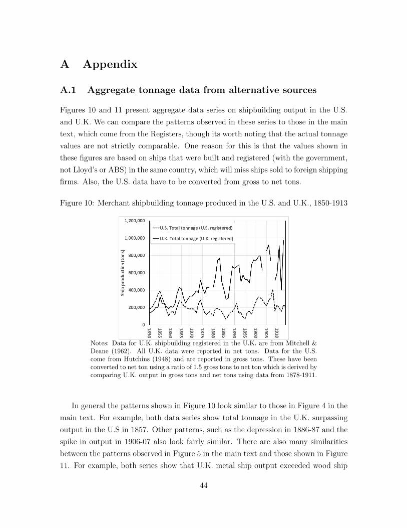
A Appendix

A.1 Aggregate tonnage data from alternative sources

Figures 10 and 11 present aggregate data series on shipbuilding output in the U.S.

and U.K. We can compare the patterns observed in these series to those in the main

text, which come from the Registers, though its worth noting that the actual tonnage

values are not strictly comparable. One reason for this is that the values shown in

these figures are based on ships that were built and registered (with the government,

not Lloyd’s or ABS) in the same country, which will miss ships sold to foreign shipping

firms. Also, the U.S. data have to be converted from gross to net tons.

Figure 10: Merchant shipbuilding tonnage produced in the U.S. and U.K., 1850-1913

Notes: Data for U.K. shipbuilding registered in the U.K. are from Mitchell &Deane (1962). All U.K. data were reported in net tons. Data for the U.S.come from Hutchins (1948) and are reported in gross tons. These have beenconverted to net ton using a ratio of 1.5 gross tons to net ton which is derived bycomparing U.K. output in gross tons and net tons using data from 1878-1911.

In general the patterns shown in Figure 10 look similar to those in Figure 4 in the

main text. For example, both data series show total tonnage in the U.K. surpassing

output in the U.S in 1857. Other patterns, such as the depression in 1886-87 and the

spike in output in 1906-07 also look fairly similar. There are also many similarities

between the patterns observed in Figure 5 in the main text and those shown in Figure

11. For example, both series show that U.K. metal ship output exceeded wood ship

44

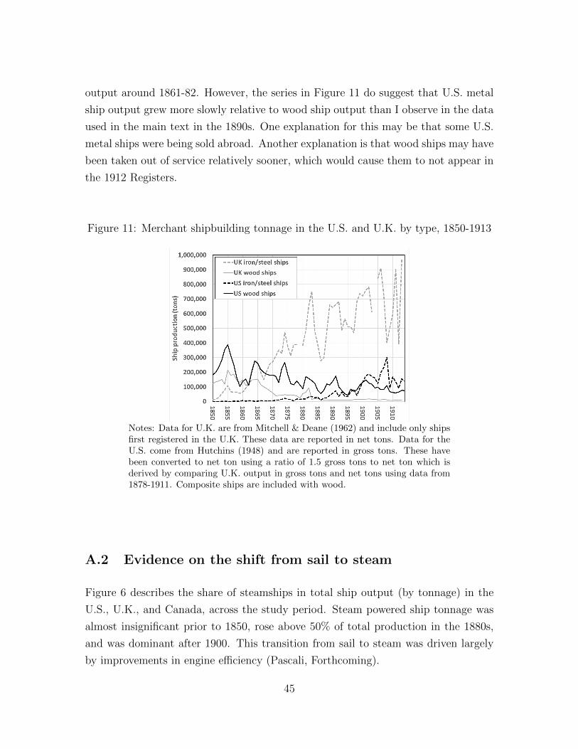
output around 1861-82. However, the series in Figure 11 do suggest that U.S. metal

ship output grew more slowly relative to wood ship output than I observe in the data

used in the main text in the 1890s. One explanation for this may be that some U.S.

metal ships were being sold abroad. Another explanation is that wood ships may have

been taken out of service relatively sooner, which would cause them to not appear in

the 1912 Registers.

Figure 11: Merchant shipbuilding tonnage in the U.S. and U.K. by type, 1850-1913

Notes: Data for U.K. are from Mitchell & Deane (1962) and include only shipsfirst registered in the U.K. These data are reported in net tons. Data for theU.S. come from Hutchins (1948) and are reported in gross tons. These havebeen converted to net ton using a ratio of 1.5 gross tons to net ton which isderived by comparing U.K. output in gross tons and net tons using data from1878-1911. Composite ships are included with wood.

A.2 Evidence on the shift from sail to steam

Figure 6 describes the share of steamships in total ship output (by tonnage) in the

U.S., U.K., and Canada, across the study period. Steam powered ship tonnage was

almost insignificant prior to 1850, rose above 50% of total production in the 1880s,

and was dominant after 1900. This transition from sail to steam was driven largely

by improvements in engine efficiency (Pascali, Forthcoming).

45

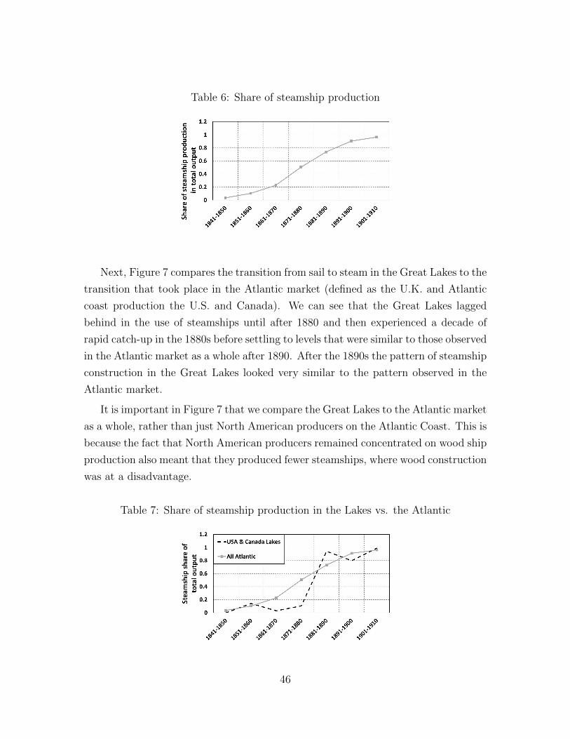
Table 6: Share of steamship production

Next, Figure 7 compares the transition from sail to steam in the Great Lakes to the

transition that took place in the Atlantic market (defined as the U.K. and Atlantic

coast production the U.S. and Canada). We can see that the Great Lakes lagged

behind in the use of steamships until after 1880 and then experienced a decade of

rapid catch-up in the 1880s before settling to levels that were similar to those observed

in the Atlantic market as a whole after 1890. After the 1890s the pattern of steamship

construction in the Great Lakes looked very similar to the pattern observed in the

Atlantic market.

It is important in Figure 7 that we compare the Great Lakes to the Atlantic market

as a whole, rather than just North American producers on the Atlantic Coast. This is

because the fact that North American producers remained concentrated on wood ship

production also meant that they produced fewer steamships, where wood construction

was at a disadvantage.

Table 7: Share of steamship production in the Lakes vs. the Atlantic

46

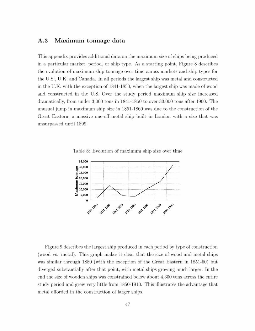
A.3 Maximum tonnage data

This appendix provides additional data on the maximum size of ships being produced

in a particular market, period, or ship type. As a starting point, Figure 8 describes

the evolution of maximum ship tonnage over time across markets and ship types for

the U.S., U.K. and Canada. In all periods the largest ship was metal and constructed

in the U.K. with the exception of 1841-1850, when the largest ship was made of wood

and constructed in the U.S. Over the study period maximum ship size increased

dramatically, from under 3,000 tons in 1841-1850 to over 30,000 tons after 1900. The

unusual jump in maximum ship size in 1851-1860 was due to the construction of the

Great Eastern, a massive one-off metal ship built in London with a size that was

unsurpassed until 1899.

Table 8: Evolution of maximum ship size over time

Figure 9 describes the largest ship produced in each period by type of construction

(wood vs. metal). This graph makes it clear that the size of wood and metal ships

was similar through 1880 (with the exception of the Great Eastern in 1851-60) but

diverged substantially after that point, with metal ships growing much larger. In the

end the size of wooden ships was constrained below about 4,300 tons across the entire

study period and grew very little from 1850-1910. This illustrates the advantage that

metal afforded in the construction of larger ships.

47

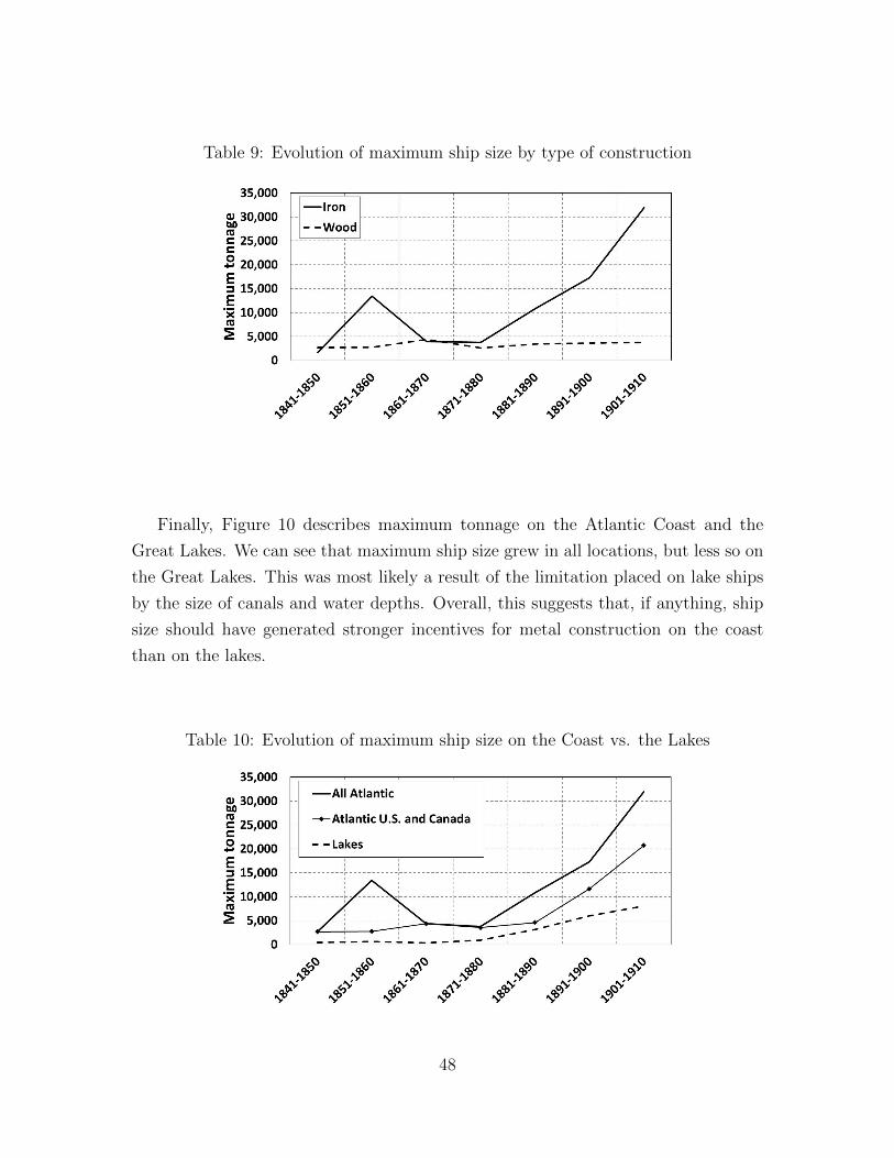
Table 9: Evolution of maximum ship size by type of construction

Finally, Figure 10 describes maximum tonnage on the Atlantic Coast and the

Great Lakes. We can see that maximum ship size grew in all locations, but less so on

the Great Lakes. This was most likely a result of the limitation placed on lake ships

by the size of canals and water depths. Overall, this suggests that, if anything, ship

size should have generated stronger incentives for metal construction on the coast

than on the lakes.

Table 10: Evolution of maximum ship size on the Coast vs. the Lakes

48

A.4 Comparing Canadian and U.S. input price trends

Figure 12 plots data describing the evolution of iron prices (top panel) and wood

prices (bottom panel) in Canada compared to the U.S. starting in the 1870s. Because

the Canadian price series are only available as an index, I convert the U.S. pig iron

price series used in Figure 1 to an index. For both indices, I set the prices from 1870-

1879 to equal one.57 These data show that the evolution of Canadian input prices

was fairly similar to the evolution of U.S. input prices across the study period.

Figure 12: Iron and wood price trends in Canada and the U.S.

Iron prices

Wood prices

Notes: U.S. prices are from Historical Statistics of the United States, Colonial Times to1870, Vol. 1. I am grateful to Ian Kaey for sharing his Canadian price series with me.

57I use a full decade here to deal with the high level of price volatility in the 1870s, which meansthat the picture can change substantially when using only a single base year.

49

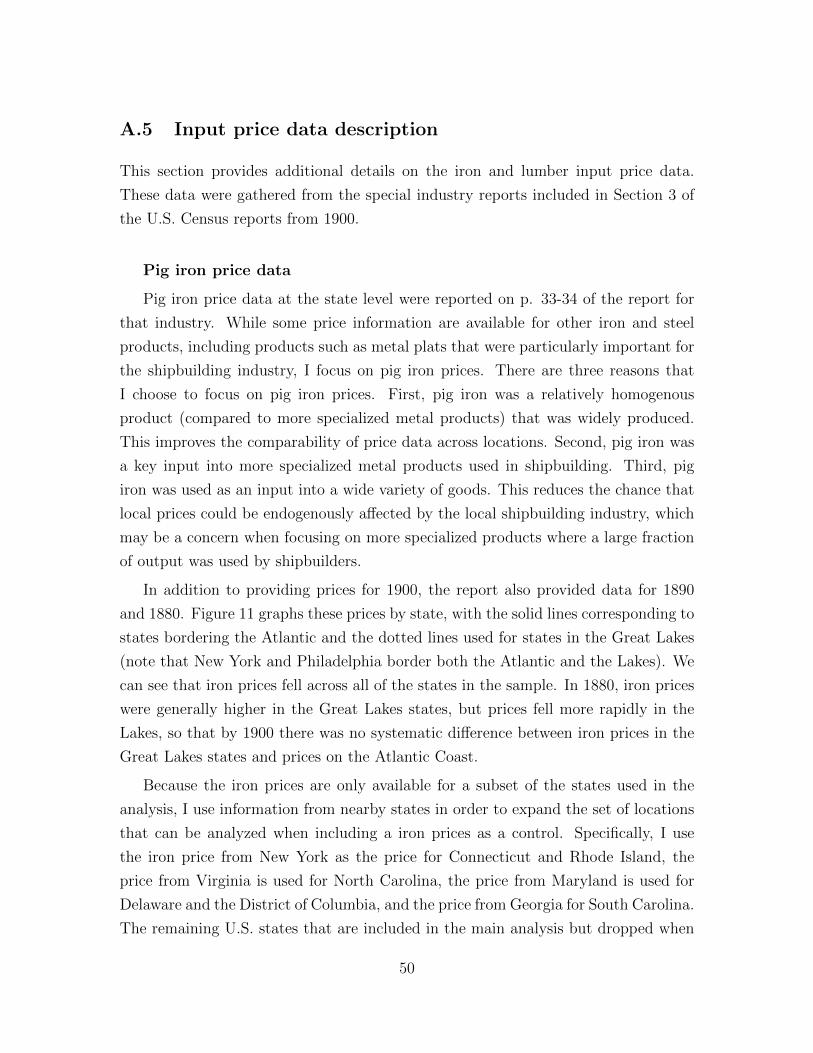
A.5 Input price data description

This section provides additional details on the iron and lumber input price data.

These data were gathered from the special industry reports included in Section 3 of

the U.S. Census reports from 1900.

Pig iron price data

Pig iron price data at the state level were reported on p. 33-34 of the report for

that industry. While some price information are available for other iron and steel

products, including products such as metal plats that were particularly important for

the shipbuilding industry, I focus on pig iron prices. There are three reasons that

I choose to focus on pig iron prices. First, pig iron was a relatively homogenous

product (compared to more specialized metal products) that was widely produced.

This improves the comparability of price data across locations. Second, pig iron was

a key input into more specialized metal products used in shipbuilding. Third, pig

iron was used as an input into a wide variety of goods. This reduces the chance that

local prices could be endogenously affected by the local shipbuilding industry, which

may be a concern when focusing on more specialized products where a large fraction

of output was used by shipbuilders.

In addition to providing prices for 1900, the report also provided data for 1890

and 1880. Figure 11 graphs these prices by state, with the solid lines corresponding to

states bordering the Atlantic and the dotted lines used for states in the Great Lakes

(note that New York and Philadelphia border both the Atlantic and the Lakes). We

can see that iron prices fell across all of the states in the sample. In 1880, iron prices

were generally higher in the Great Lakes states, but prices fell more rapidly in the

Lakes, so that by 1900 there was no systematic difference between iron prices in the

Great Lakes states and prices on the Atlantic Coast.

Because the iron prices are only available for a subset of the states used in the

analysis, I use information from nearby states in order to expand the set of locations

that can be analyzed when including a iron prices as a control. Specifically, I use

the iron price from New York as the price for Connecticut and Rhode Island, the

price from Virginia is used for North Carolina, the price from Maryland is used for

Delaware and the District of Columbia, and the price from Georgia for South Carolina.

The remaining U.S. states that are included in the main analysis but dropped when

50

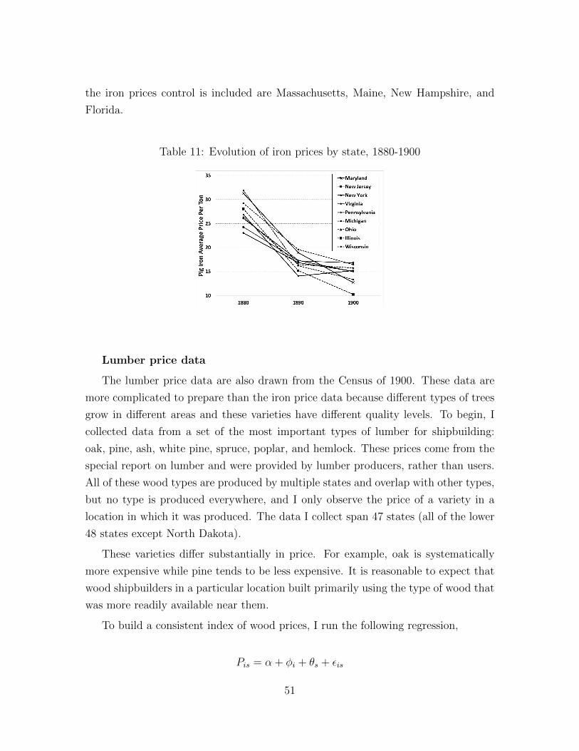
the iron prices control is included are Massachusetts, Maine, New Hampshire, and

Florida.

Table 11: Evolution of iron prices by state, 1880-1900

Lumber price data

The lumber price data are also drawn from the Census of 1900. These data are

more complicated to prepare than the iron price data because different types of trees

grow in different areas and these varieties have different quality levels. To begin, I

collected data from a set of the most important types of lumber for shipbuilding:

oak, pine, ash, white pine, spruce, poplar, and hemlock. These prices come from the

special report on lumber and were provided by lumber producers, rather than users.

All of these wood types are produced by multiple states and overlap with other types,

but no type is produced everywhere, and I only observe the price of a variety in a

location in which it was produced. The data I collect span 47 states (all of the lower

48 states except North Dakota).

These varieties differ substantially in price. For example, oak is systematically

more expensive while pine tends to be less expensive. It is reasonable to expect that

wood shipbuilders in a particular location built primarily using the type of wood that

was more readily available near them.

To build a consistent index of wood prices, I run the following regression,

Pis = α + φi + θs + εis

51

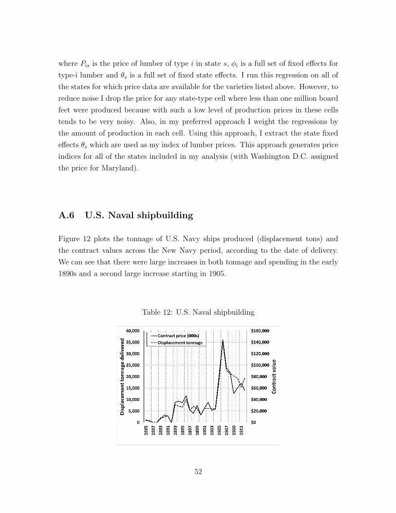
where Pis is the price of lumber of type i in state s, φi is a full set of fixed effects for

type-i lumber and θs is a full set of fixed state effects. I run this regression on all of

the states for which price data are available for the varieties listed above. However, to

reduce noise I drop the price for any state-type cell where less than one million board

feet were produced because with such a low level of production prices in these cells

tends to be very noisy. Also, in my preferred approach I weight the regressions by

the amount of production in each cell. Using this approach, I extract the state fixed

effects θs which are used as my index of lumber prices. This approach generates price

indices for all of the states included in my analysis (with Washington D.C. assigned

the price for Maryland).

A.6 U.S. Naval shipbuilding

Figure 12 plots the tonnage of U.S. Navy ships produced (displacement tons) and

the contract values across the New Navy period, according to the date of delivery.

We can see that there were large increases in both tonnage and spending in the early

1890s and a second large increase starting in 1905.

Table 12: U.S. Naval shipbuilding

52

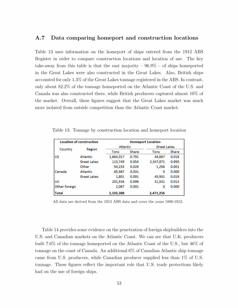
A.7 Data comparing homeport and construction locations

Table 13 uses information on the homeport of ships entered from the 1912 ABS

Register in order to compare construction locations and location of use. The key

take-away from this table is that the vast majority – 96.9% – of ships homeported

in the Great Lakes were also constructed in the Great Lakes. Also, British ships

accounted for only 1.3% of the Great Lakes tonnage registered in the ABS. In contrast,

only about 82.2% of the tonnage homeported on the Atlantic Coast of the U.S. and

Canada was also constructed there, while British producers captured almost 10% of

the market. Overall, these figures suggest that the Great Lakes market was much

more isolated from outside competition than the Atlantic Coast market.

Table 13: Tonnage by construction location and homeport location

All data are derived from the 1912 ABS data and cover the years 1890-1912.

Table 14 provides some evidence on the penetration of foreign shipbuilders into the

U.S. and Canadian markets on the Atlantic Coast. We can see that U.K. producers

built 7.6% of the tonnage homeported on the Atlantic Coast of the U.S., but 46% of

tonnage on the coast of Canada. An additional 6% of Canadian Atlantic ship tonnage

came from U.S. producers, while Canadian producer supplied less than 1% of U.S.

tonnage. These figures reflect the important role that U.S. trade protections likely

had on the use of foreign ships.

53

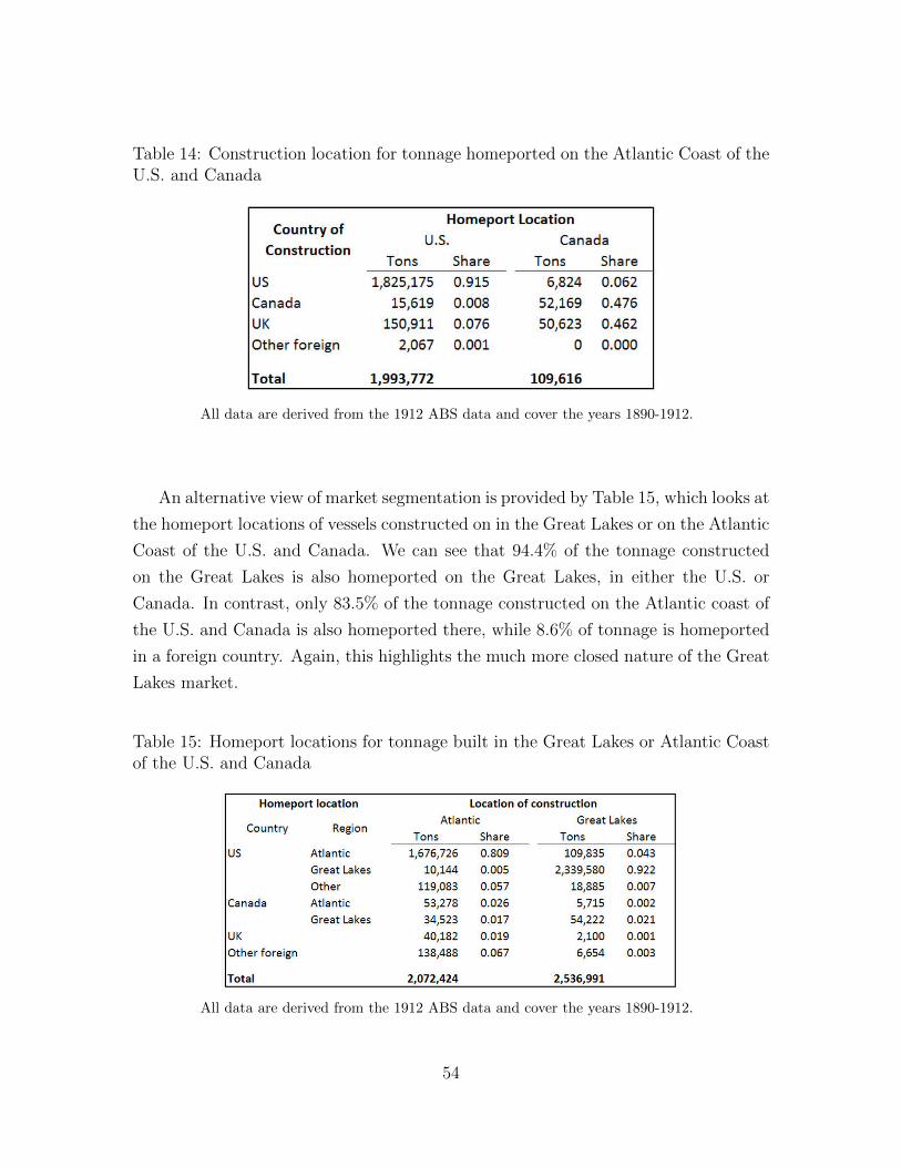
Table 14: Construction location for tonnage homeported on the Atlantic Coast of theU.S. and Canada

All data are derived from the 1912 ABS data and cover the years 1890-1912.

An alternative view of market segmentation is provided by Table 15, which looks at

the homeport locations of vessels constructed on in the Great Lakes or on the Atlantic

Coast of the U.S. and Canada. We can see that 94.4% of the tonnage constructed

on the Great Lakes is also homeported on the Great Lakes, in either the U.S. or

Canada. In contrast, only 83.5% of the tonnage constructed on the Atlantic coast of

the U.S. and Canada is also homeported there, while 8.6% of tonnage is homeported

in a foreign country. Again, this highlights the much more closed nature of the Great

Lakes market.

Table 15: Homeport locations for tonnage built in the Great Lakes or Atlantic Coastof the U.S. and Canada

All data are derived from the 1912 ABS data and cover the years 1890-1912.

54

A.8 Additional results for whether a location is active

This section presents some additional results looking at the factors that predict

whether a location was active in producing a particular type of ship (wood or metal)

in the 1901-1910 period. The first table of results covers the same specifications shown

in the main text but includes estimates for all of the control variables. There are a few

coefficient estimates worth discussing among the control variables. The one control

variable with the greatest predictive power the the tonnage of wood ship production

in the 1870s, which is positively related to output in all types of ships later on. Since

wood was by far the dominant type of production in the 1870s, this can essentially

be thought of as capturing the impact of overall production in the 1870s. Thus, this

variable is most likely reflecting factors that determine the shipbuilding capacity of

the location, such as the quality of the harbor or the availability of flat shipyard land

with harbor access. None of the other control variables show clear patterns.

Next, I present some additional multinomial logit regression results that allow the

production of sail vs. steam ships to be different choices. Thus, the outcome variable

can take five values: 0 if the location was inactive; 1 if the location produced wood

sailing ships; 2 if the location produced wood steamships; 3 if the location produced

metal sailing ships; 4 if the location produced metal steamships. To keep things

tractable, I treat these as independent decisions. This differs from the specification

used in the main text, which considers the joint production of iron and wood ships

to be a different choice than producing only iron.

One reason to consider this specification is that we may be concerned that differ-

ences in the use of steamships between the Great Lakes and Coastal regions may have

contributed to differences in the use of metal vs. wood for construction. Looking at

the effect of being in the Great Lakes on production of metal vs. wood ships within

ship type can address this potential concern. However, because we are dividing the

data into smaller cells we should expect this specification to deliver results with larger

standard errors.

Table 17 presents ML regression results differentiating by both material of con-

struction and power source. Note that these results do not include the specifications

with controls for the iron and lumber prices. Doing so reduces the sample size and

makes it difficult to estimate reliable results when using more categories.

55

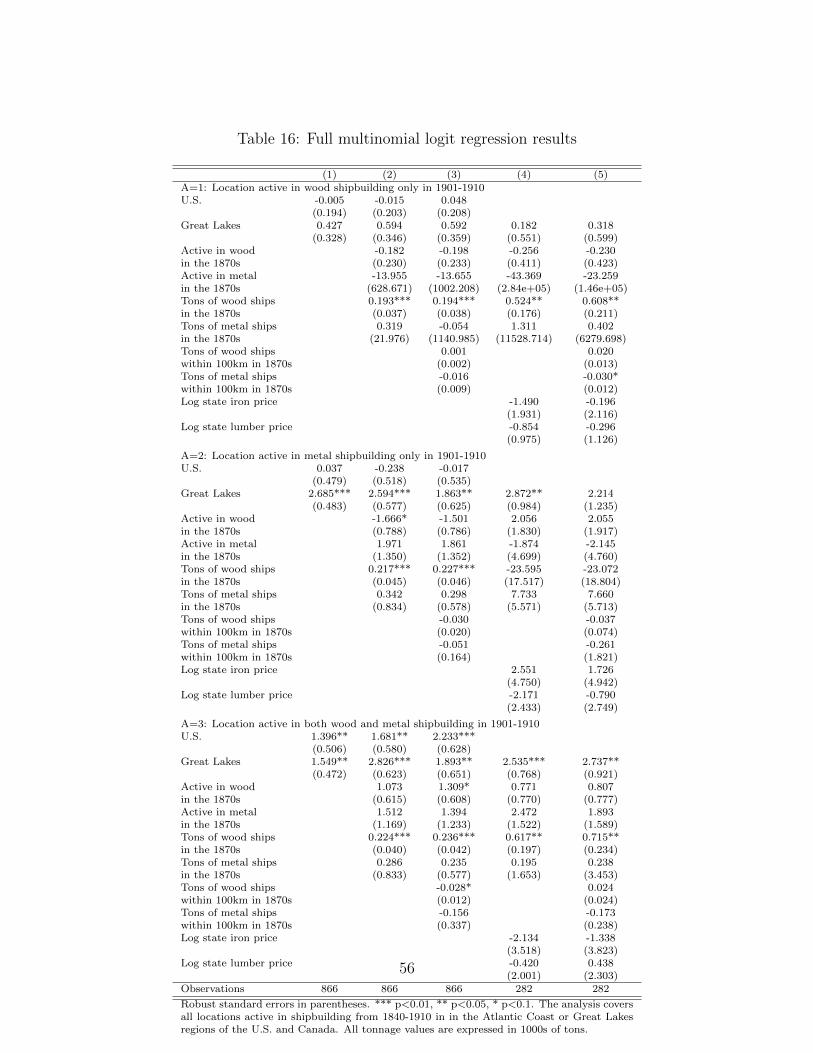
Table 16: Full multinomial logit regression results

(1) (2) (3) (4) (5)A=1: Location active in wood shipbuilding only in 1901-1910U.S. -0.005 -0.015 0.048

(0.194) (0.203) (0.208)Great Lakes 0.427 0.594 0.592 0.182 0.318

(0.328) (0.346) (0.359) (0.551) (0.599)Active in wood -0.182 -0.198 -0.256 -0.230in the 1870s (0.230) (0.233) (0.411) (0.423)Active in metal -13.955 -13.655 -43.369 -23.259in the 1870s (628.671) (1002.208) (2.84e+05) (1.46e+05)Tons of wood ships 0.193*** 0.194*** 0.524** 0.608**in the 1870s (0.037) (0.038) (0.176) (0.211)Tons of metal ships 0.319 -0.054 1.311 0.402in the 1870s (21.976) (1140.985) (11528.714) (6279.698)Tons of wood ships 0.001 0.020within 100km in 1870s (0.002) (0.013)Tons of metal ships -0.016 -0.030*within 100km in 1870s (0.009) (0.012)Log state iron price -1.490 -0.196

(1.931) (2.116)Log state lumber price -0.854 -0.296

(0.975) (1.126)

A=2: Location active in metal shipbuilding only in 1901-1910U.S. 0.037 -0.238 -0.017

(0.479) (0.518) (0.535)Great Lakes 2.685*** 2.594*** 1.863** 2.872** 2.214

(0.483) (0.577) (0.625) (0.984) (1.235)Active in wood -1.666* -1.501 2.056 2.055in the 1870s (0.788) (0.786) (1.830) (1.917)Active in metal 1.971 1.861 -1.874 -2.145in the 1870s (1.350) (1.352) (4.699) (4.760)Tons of wood ships 0.217*** 0.227*** -23.595 -23.072in the 1870s (0.045) (0.046) (17.517) (18.804)Tons of metal ships 0.342 0.298 7.733 7.660in the 1870s (0.834) (0.578) (5.571) (5.713)Tons of wood ships -0.030 -0.037within 100km in 1870s (0.020) (0.074)Tons of metal ships -0.051 -0.261within 100km in 1870s (0.164) (1.821)Log state iron price 2.551 1.726

(4.750) (4.942)Log state lumber price -2.171 -0.790

(2.433) (2.749)

A=3: Location active in both wood and metal shipbuilding in 1901-1910U.S. 1.396** 1.681** 2.233***

(0.506) (0.580) (0.628)Great Lakes 1.549** 2.826*** 1.893** 2.535*** 2.737**

(0.472) (0.623) (0.651) (0.768) (0.921)Active in wood 1.073 1.309* 0.771 0.807in the 1870s (0.615) (0.608) (0.770) (0.777)Active in metal 1.512 1.394 2.472 1.893in the 1870s (1.169) (1.233) (1.522) (1.589)Tons of wood ships 0.224*** 0.236*** 0.617** 0.715**in the 1870s (0.040) (0.042) (0.197) (0.234)Tons of metal ships 0.286 0.235 0.195 0.238in the 1870s (0.833) (0.577) (1.653) (3.453)Tons of wood ships -0.028* 0.024within 100km in 1870s (0.012) (0.024)Tons of metal ships -0.156 -0.173within 100km in 1870s (0.337) (0.238)Log state iron price -2.134 -1.338

(3.518) (3.823)Log state lumber price -0.420 0.438

(2.001) (2.303)Observations 866 866 866 282 282

Robust standard errors in parentheses. *** p<0.01, ** p<0.05, * p<0.1. The analysis coversall locations active in shipbuilding from 1840-1910 in in the Atlantic Coast or Great Lakesregions of the U.S. and Canada. All tonnage values are expressed in 1000s of tons.

56

In the top panel, we see that shipbuilders in the Great Lakes or in the U.S. were

not more likely to be active in building wood sailing ships. In the second panel,

we see evidence that both Great Lakes and U.S. shipbuilders were more likely to

be active in the construction of wood steamships. In the third panel we see some

evidence that Great Lakes producers were more likely to be active in metal sailing

ship production, though with few ships falling into this category the results are not

statistically significant. In the fourth panel, the results show that both the Great

Lakes and U.S. locations were more likely to be active in metal steamship production.

This result indicates that my main results hold when looking only within steamships.

57

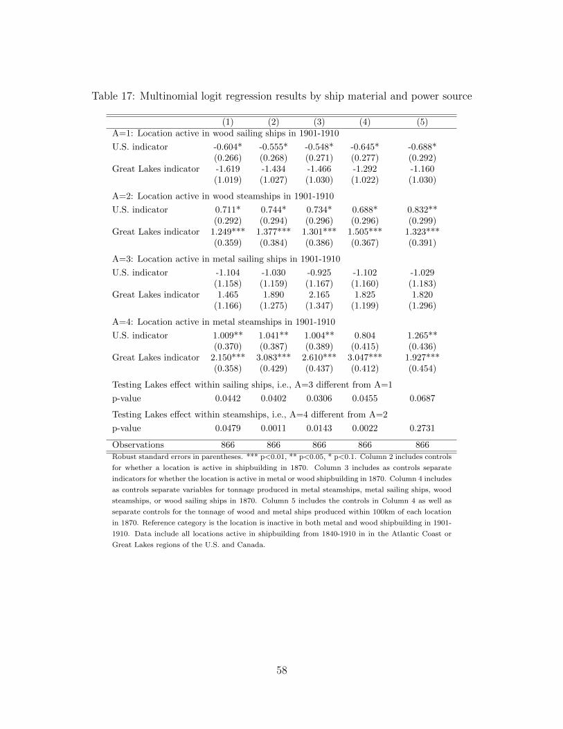
Table 17: Multinomial logit regression results by ship material and power source

(1) (2) (3) (4) (5)A=1: Location active in wood sailing ships in 1901-1910

U.S. indicator -0.604* -0.555* -0.548* -0.645* -0.688*(0.266) (0.268) (0.271) (0.277) (0.292)

Great Lakes indicator -1.619 -1.434 -1.466 -1.292 -1.160(1.019) (1.027) (1.030) (1.022) (1.030)

A=2: Location active in wood steamships in 1901-1910

U.S. indicator 0.711* 0.744* 0.734* 0.688* 0.832**(0.292) (0.294) (0.296) (0.296) (0.299)

Great Lakes indicator 1.249*** 1.377*** 1.301*** 1.505*** 1.323***(0.359) (0.384) (0.386) (0.367) (0.391)

A=3: Location active in metal sailing ships in 1901-1910

U.S. indicator -1.104 -1.030 -0.925 -1.102 -1.029(1.158) (1.159) (1.167) (1.160) (1.183)

Great Lakes indicator 1.465 1.890 2.165 1.825 1.820(1.166) (1.275) (1.347) (1.199) (1.296)

A=4: Location active in metal steamships in 1901-1910

U.S. indicator 1.009** 1.041** 1.004** 0.804 1.265**(0.370) (0.387) (0.389) (0.415) (0.436)

Great Lakes indicator 2.150*** 3.083*** 2.610*** 3.047*** 1.927***(0.358) (0.429) (0.437) (0.412) (0.454)

Testing Lakes effect within sailing ships, i.e., A=3 different from A=1

p-value 0.0442 0.0402 0.0306 0.0455 0.0687

Testing Lakes effect within steamships, i.e., A=4 different from A=2

p-value 0.0479 0.0011 0.0143 0.0022 0.2731

Observations 866 866 866 866 866Robust standard errors in parentheses. *** p<0.01, ** p<0.05, * p<0.1. Column 2 includes controls

for whether a location is active in shipbuilding in 1870. Column 3 includes as controls separate

indicators for whether the location is active in metal or wood shipbuilding in 1870. Column 4 includes

as controls separate variables for tonnage produced in metal steamships, metal sailing ships, wood

steamships, or wood sailing ships in 1870. Column 5 includes the controls in Column 4 as well as

separate controls for the tonnage of wood and metal ships produced within 100km of each location

in 1870. Reference category is the location is inactive in both metal and wood shipbuilding in 1901-

1910. Data include all locations active in shipbuilding from 1840-1910 in in the Atlantic Coast or

Great Lakes regions of the U.S. and Canada.

58

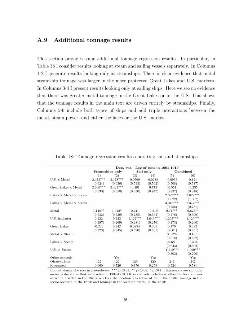
A.9 Additional tonnage results

This section provides some additional tonnage regression results. In particular, in

Table 18 I consider results looking at steam and sailing vessels separately. In Columns

1-2 I generate results looking only at steamships. There is clear evidence that metal

steamship tonnage was larger in the more protected Great Lakes and U.S. markets.

In Columns 3-4 I present results looking only at sailing ships. Here we see no evidence

that there was greater metal tonnage in the Great Lakes or in the U.S. This shows

that the tonnage results in the main text are driven entirely by steamships. Finally,

Columns 5-6 include both types of ships and add triple interactions between the

metal, steam power, and either the lakes or the U.S. market.

Table 18: Tonnage regression results separating sail and steamships

Dep. var.: Log of tons in 1901-1910Steamships only Sail only Combined(1) (2) (3) (4) (5) (6)

U.S. x Metal 2.473*** 2.178*** 0.0769 0.0288 -0.0955 0.121(0.624) (0.636) (0.513) (0.502) (0.508) (0.517)

Great Lakes x Metal 2.006*** 2.421*** -0.461 0.772 -0.551 -0.235(0.630) (0.650) (0.830) (0.947) (0.837) (0.848)

Lakes × Metal × Steam 2.822*** 2.622***(1.022) (1.007)

Lakes × Metal × Steam 3.015*** 2.377***(0.758) (0.781)

Metal 1.118** 1.012* 0.441 -0.519 0.617** 0.625**(0.532) (0.539) (0.285) (0.554) (0.276) (0.309)

U.S. indicator 0.222 0.223 1.122*** 1.049*** 1.295*** 1.120***(0.297) (0.269) (0.281) (0.276) (0.273) (0.266)

Great Lakes -0.236 0.242 0.0894 0.331 0.179 0.492(0.323) (0.345) (0.590) (0.561) (0.601) (0.551)

Metal × Steam 0.0126 0.181(0.518) (0.522)

Lakes × Steam -0.680 -0.546(0.643) (0.602)

U.S. × Steam -1.519*** -1.069***(0.302) (0.296)

Other controls Yes Yes YesObservations 122 122 120 120 242 242R-squared 0.660 0.726 0.176 0.259 0.524 0.581

Robust standard errors in parentheses. *** p<0.01, ** p<0.05, * p<0.1. Regressions are run onlyon sector-locations that were active in 1901-1910. Other controls includes whether the location wasactive in a sector in the 1870s, whether the location was active at all in the 1870s, tonnage in thesector-location in the 1870s and tonnage in the location overall in the 1870s.

59

A.10 Separated results

This appendix provides results for regressions run separately on the U.S. and Canada

(looking at the effect of being in the Lakes) or run separately on the Lakes and

Atlantic Coast (looking at the effect of being in the U.S.). If the main function of the

Great Lakes is to provide protection from foreign competition, then we should expect

this to have an impact in both the U.S. and in Canada.

I begin, in Table 19, by presenting multinomial logit results looking at whether a

location is active in wood shipbuilding, metal shipbuilding, or both. The results in

Columns 1-2 look at, respectively, the U.S. and Canada separately. These show that

locations in the Great Lakes were more likely to be active in metal shipbuilding, either

alone or in combination with wood shipbuilding, but not in wood shipbuilding alone.

The point estimates are similar whether we look at the U.S. or Canada, though the

standard errors on the Canadian estimates are larger such that those are not always

statistically significant.

Columns 3-4 present separate results for, respectively, the Atlantic and Lakes,

looking at the impact of locations being located in the U.S. Here we see some evidence

that locations in the U.S. were more likely to be active in both metal and wood

shipbuilding, though these results are not strongly statistically significant. It is worth

noting here that we should not expect the effect of being in the U.S. to be zero on

the Great Lakes just because the Lakes are protected from British competition, since

protective U.S. policies may still be having an effect even in the absence of British

competition.

Table 20 presents a similar set of results but using the log tonnage specification

from Eq. 2. These results show that, conditional on being active in 1901-1910, loca-

tions in the Great Lakes produced more metal shipping in both the U.S. (Column 1)

and Canada (Column 2). In Columns 3-4 we see that locations in the more protected

U.S. market produced more metal ship tonnage on both the Atlantic Coast and the

Lakes.

60

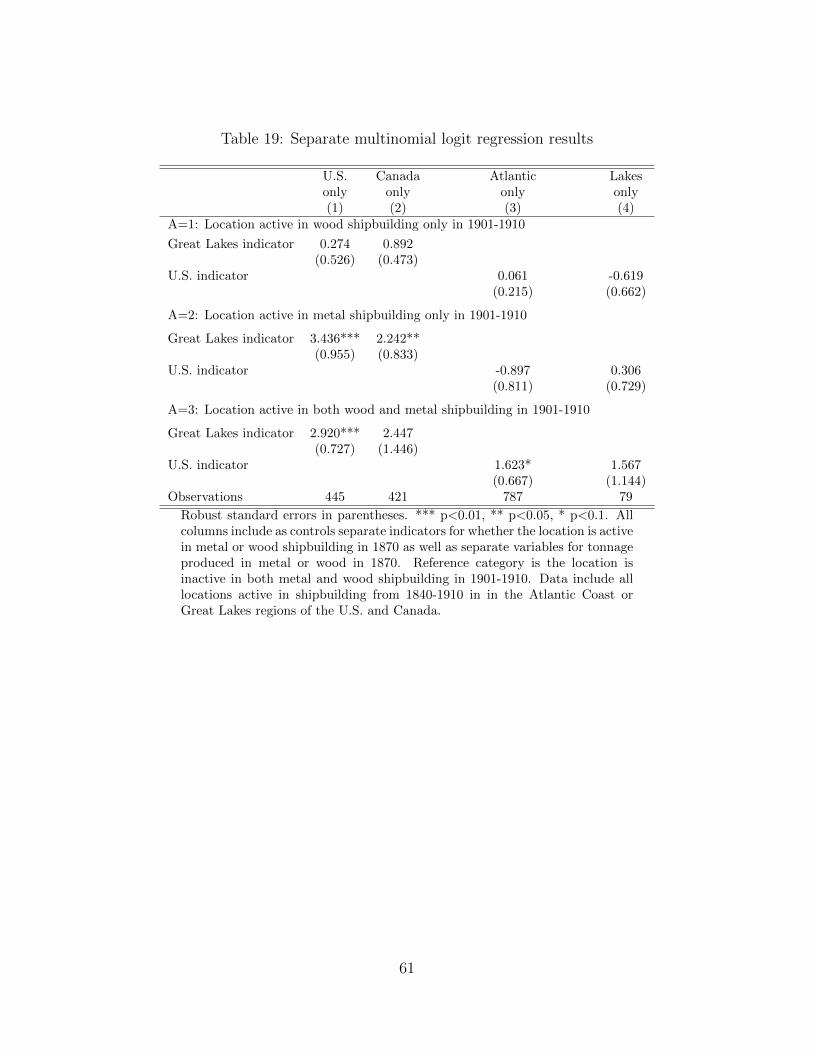
Table 19: Separate multinomial logit regression results

U.S. Canada Atlantic Lakesonly only only only(1) (2) (3) (4)

A=1: Location active in wood shipbuilding only in 1901-1910

Great Lakes indicator 0.274 0.892(0.526) (0.473)

U.S. indicator 0.061 -0.619(0.215) (0.662)

A=2: Location active in metal shipbuilding only in 1901-1910

Great Lakes indicator 3.436*** 2.242**(0.955) (0.833)

U.S. indicator -0.897 0.306(0.811) (0.729)

A=3: Location active in both wood and metal shipbuilding in 1901-1910

Great Lakes indicator 2.920*** 2.447(0.727) (1.446)

U.S. indicator 1.623* 1.567(0.667) (1.144)

Observations 445 421 787 79

Robust standard errors in parentheses. *** p<0.01, ** p<0.05, * p<0.1. Allcolumns include as controls separate indicators for whether the location is activein metal or wood shipbuilding in 1870 as well as separate variables for tonnageproduced in metal or wood in 1870. Reference category is the location isinactive in both metal and wood shipbuilding in 1901-1910. Data include alllocations active in shipbuilding from 1840-1910 in in the Atlantic Coast orGreat Lakes regions of the U.S. and Canada.

61

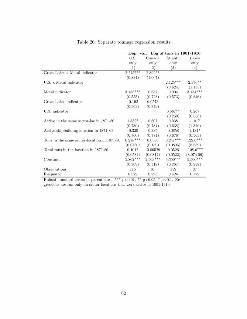
Table 20: Separate tonnage regression results

Dep. var.: Log of tons in 1901-1910U.S. Canada Atlantic Lakesonly only only only(1) (2) (3) (4)

Great Lakes x Metal indicator 2.245*** 2.392**(0.834) (1.067)

U.S. x Metal indicator 2.125*** 2.376**(0.624) (1.135)

Metal indicator 3.185*** 0.687 0.904 3.134***(0.555) (0.728) (0.573) (0.846)

Great Lakes indicator -0.192 0.0573(0.563) (0.349)

U.S. indicator 0.567** 0.207(0.250) (0.558)

Active in the same sector-loc in 1871-80 1.332* 0.607 0.938 -1.017(0.730) (0.784) (0.638) (1.346)

Active shipbuilding location in 1871-80 -0.320 0.335 0.0658 1.131*(0.760) (0.784) (0.676) (0.563)

Tons in the same sector-location in 1871-80 0.278*** 0.0568 0.247*** 122.6***(0.0750) (0.139) (0.0805) (8.859)

Total tons in the location in 1871-80 0.101* -0.00529 0.0526 -108.6***(0.0584) (0.0812) (0.0522) (8.07e-06)

Constant 5.862*** 5.503*** 5.350*** 5.506***(0.309) (0.318) (0.267) (0.238)

Observations 115 81 159 37R-squared 0.572 0.293 0.426 0.772

Robust standard errors in parentheses. *** p<0.01, ** p<0.05, * p<0.1. Re-gressions are run only on sector-locations that were active in 1901-1910.

62