Statistical Science2013, Vol. 28, No. 2, 238–256DOI: 10.1214/13-STS414© Institute of Mathematical Statistics, 2013

Handling Attrition in Longitudinal Studies:The Case for Refreshment SamplesYiting Deng, D. Sunshine Hillygus, Jerome P. Reiter, Yajuan Si and Siyu Zheng

Abstract. Panel studies typically suffer from attrition, which reduces sam-ple size and can result in biased inferences. It is impossible to know whetheror not the attrition causes bias from the observed panel data alone. Refresh-ment samples—new, randomly sampled respondents given the questionnaireat the same time as a subsequent wave of the panel—offer information thatcan be used to diagnose and adjust for bias due to attrition. We review andbolster the case for the use of refreshment samples in panel studies. We in-clude examples of both a fully Bayesian approach for analyzing the con-catenated panel and refreshment data, and a multiple imputation approachfor analyzing only the original panel. For the latter, we document a positivebias in the usual multiple imputation variance estimator. We present modelsappropriate for three waves and two refreshment samples, including nonter-minal attrition. We illustrate the three-wave analysis using the 2007–2008Associated Press–Yahoo! News Election Poll.

Key words and phrases: Attrition, imputation, missing, panel, survey.

1. INTRODUCTION

Many of the the major ongoing government orgovernment-funded surveys have panel components in-cluding, for example, in the U.S., the American Na-tional Election Study (ANES), the General Social Sur-vey (GSS), the Panel Survey on Income Dynamics(PSID) and the Current Population Survey (CPS). De-spite the millions of dollars spent each year to col-lect high quality data, analyses using panel data areinevitably threatened by panel attrition (Lynn, 2009),that is, some respondents in the sample do not par-ticipate in later waves of the study because they can-

Yiting Deng is Ph.D. Candidate, Fuqua School of Business,Duke University, Box 90120, Durham, North Carolina27708, USA (e-mail: yiting.deng@duke.edu). D. SunshineHillygus is Associate Professor, Department of PoliticalScience, Duke University, Box 90204, Durham, NorthCarolina 27708, USA (e-mail: hillygus@duke.edu). JeromeP. Reiter is Professor and Siyu Zheng is B.S. Alumnus,Department of Statistical Science, Duke University, Box90251, Durham, North Carolina 27708, USA (e-mail:jerry@stat.duke.edu; s.zheng@alumni.duke.edu). Yajuan Siis Postdoctoral Associate, Applied Statistical Center,Columbia University, 1255 Amsterdam Avenue, New York,New York 10027, USA (e-mail: yajuan.si@columbia.edu).

not be located or refuse participation. For instance, themultiple-decade PSID, first fielded in 1968, lost nearly50 percent of the initial sample members by 1989due to cumulative attrition and mortality. Even witha much shorter study period, the 2008–2009 ANESPanel Study, which conducted monthly interviews overthe course of the 2008 election cycle, lost 36 percentof respondents in less than a year.

At these rates, which are not atypical in large-scalepanel studies, attrition can have serious impacts onanalyses that use only respondents who completed allwaves of the survey. At best, attrition reduces effec-tive sample size, thereby decreasing analysts’ abilitiesto discover longitudinal trends in behavior. At worst,attrition results in an available sample that is not repre-sentative of the target population, thereby introducingpotentially substantial biases into statistical inferences.It is not possible for analysts to determine the degreeto which attrition degrades complete-case analyses byusing only the collected data; external sources of infor-mation are needed.

One such source is refreshment samples. A refresh-ment sample includes new, randomly sampled respon-dents who are given the questionnaire at the same timeas a second or subsequent wave of the panel. Many

238

REFRESHMENT SAMPLES AND ATTRITION 239

of the large panel studies now routinely include re-freshment samples. For example, most of the longerlongitudinal studies of the National Center for Educa-tion Statistics, including the Early Childhood Longi-tudinal Study and the National Educational Longitu-dinal Study, freshened their samples at some point inthe study, either adding new panelists or as a separatecross-section. The National Educational LongitudinalStudy, for instance, followed 21,500 eighth graders intwo-year intervals until 2000 and included refreshmentsamples in 1990 and 1992. It is worth noting that by thefinal wave of data collection, just 50% of the originalsample remained in the panel. Overlapping or rotatingpanel designs offer the equivalent of refreshment sam-ples. In such designs, the sample is divided into dif-ferent cohorts with staggered start times such that onecohort of panelists completes a follow-up interview atthe same time another cohort completes their baselineinterview. So long as each cohort is randomly selectedand administered the same questionnaire, the baselineinterview of the new cohort functions as a refreshmentsample for the old cohort. Examples of such rotatingpanel designs include the GSS and the Survey of In-come and Program Participation.

Refreshment samples provide information that canbe used to assess the effects of panel attrition andto correct for biases via statistical modeling (Hiranoet al., 1998). However, they are infrequently used byanalysts or data collectors for these tasks. In mostcases, attrition is simply ignored, with the analysis runonly on those respondents who completed all wavesof the study (e.g., Jelicic, Phelps and Lerner, 2009),perhaps with the use of post-stratification weights(Vandecasteele and Debels, 2007). This is done despitewidespread recognition among subject matter expertsabout the potential problems of panel attrition (e.g.,Ahern and Le Brocque, 2005).

In this article, we review and bolster the case forthe use of refreshment samples in panel studies. Webegin in Section 2 by briefly describing existing ap-proaches for handling attrition that do not involve re-freshment samples. In Section 3 we present a hypo-thetical two-wave panel to illustrate how refreshmentsamples can be used to remove bias from nonignorableattrition. In Section 4 we extend current models forrefreshment samples, which are described exclusivelywith two-wave settings in the literature, to models forthree waves and two refreshment samples. In doing so,we discuss modeling nonterminal attrition in these set-tings, which arises when respondents fail to respond toone wave but return to the study for a subsequent one.

In Section 5 we illustrate the three-wave analysis usingthe 2007–2008 Associated Press–Yahoo! News Elec-tion Poll (APYN), which is a panel study of the 2008U.S. Presidential election. Finally, in Section 6 we dis-cuss some limitations and open research issues in theuse of refreshment samples.

2. PANEL ATTRITION IN LONGITUDINAL STUDIES

Fundamentally, panel attrition is a problem of nonre-sponse, so it is useful to frame the various approachesto handling panel attrition based on the assumed miss-ing data mechanisms (Rubin, 1976; Little and Rubin,2002). Often researchers ignore panel attrition entirelyand use only the available cases for analysis, for ex-ample, listwise deletion to create a balanced subpanel(e.g., Bartels, 1993; Wawro, 2002). Such approachesassume that the panel attrition is missing completely atrandom (MCAR), that is, the missingness is indepen-dent of observed and unobserved data. We speculatethat this is usually assumed for convenience, as oftenlistwise deletion analyses are not presented with em-pirical justification of MCAR assumptions. To the ex-tent that diagnostic analyses of MCAR assumptions inpanel attrition are conducted, they tend to be reportedand published separately from the substantive research(e.g., Zabel, 1998; Fitzgerald, Gottschalk and Moffitt,1998; Bartels, 1999; Clinton, 2001; Kruse et al., 2009),so that it is not clear if and how the diagnostics influ-ence statistical model specification.

Considerable research has documented that some in-dividuals are more likely to drop out than others (e.g.,Behr, Bellgardt and Rendtel, 2005; Olsen, 2005), mak-ing listwise deletion a risky analysis strategy. Manyanalysts instead assume that the data are missing at ran-dom (MAR), that is, missingness depends on observed,but not unobserved, data. One widely used MAR ap-proach is to adjust survey weights for nonresponse, forexample, by using post-stratification weights providedby the survey organization (e.g., Henderson, Hillygusand Tompson, 2010). Re-weighting approaches assumethat dropout occurs randomly within weighting classesdefined by observed variables that are associated withdropout.

Although re-weighting can reduce bias introducedby panel attrition, it is not a fail-safe solution. Thereis wide variability in the way weights are constructedand in the variables used. Nonresponse weights are of-ten created using demographic benchmarks, for exam-ple, from the CPS, but demographic variables aloneare unlikely to be adequate to correct for attrition

240 Y. DENG ET AL.

(Vandecasteele and Debels, 2007). As is the case inother nonresponse contexts, inflating weights can re-sult in increased standard errors and introduce instabil-ities due to particularly large or small weights (Lohr,1998; Gelman, 2007).

A related MAR approach uses predicted probabil-ities of nonresponse, obtained by modeling the re-sponse indicator as a function of observed variables,as inverse probability weights to enable inference bygeneralized estimating equations (e.g., Robins andRotnitzky, 1995; Robins, Rotnitzky and Zhao, 1995;Scharfstein, Rotnitzky and Robins, 1999; Chen, Yi andCook, 2010). This potentially offers some robustnessto model misspecification, at least asymptotically forMAR mechanisms, although inferences can be sen-sitive to large weights. One also can test whether ornot parameters differ significantly due to attrition forcases with complete data and cases with incompletedata (e.g., Diggle, 1989; Chen and Little, 1999; Qu andSong, 2002; Qu et al., 2011), which can offer insightinto the appropriateness of the assumed MAR mecha-nism.

An alternative approach to re-weighting is single im-putation, a method often applied by statistical agen-cies in general item nonresponse contexts (Kalton andKasprzyk, 1986). Single imputation methods replaceeach missing value with a plausible guess, so thatthe full panel can be analyzed as if their data werecomplete. Although there are a wide range of singleimputation methods (hot deck, nearest neighbor, etc.)that have been applied to missing data problems, themethod most specific to longitudinal studies is the last-observation-carried-forward approach, in which an in-dividual’s missing data are imputed to equal his or herresponse in previous waves (e.g., Packer et al., 1996).Research has shown that this approach can introducesubstantial biases in inferences (e.g., see Daniels andHogan, 2008).

Given the well-known limitations of single imputa-tion methods (Little and Rubin, 2002), multiple im-putation (see Section 3) also has been used to handlemissing data from attrition (e.g., Pasek et al., 2009;Honaker and King, 2010). As with the majority ofavailable methods used to correct for panel attrition,standard approaches to multiple imputation assume anignorable missing data mechanism. Unfortunately, it isoften expected that panel attrition is not missing at ran-dom (NMAR), that is, the missingness depends on un-observed data. In such cases, the only way to obtainunbiased estimates of parameters is to model the miss-ingness. However, it is generally impossible to know

the appropriate model for the missingness mechanismfrom the panel sample alone (Kristman, Manno andCote, 2005; Basic and Rendtel, 2007; Molenberghset al., 2008).

Another approach, absent external data, is to han-dle the attrition directly in the statistical models usedfor longitudinal data analysis (Verbeke and Molen-berghs, 2000; Diggle et al., 2002; Fitzmaurice, Lairdand Ware, 2004; Hedeker and Gibbons, 2006; Danielsand Hogan, 2008). Here, unlike with other approaches,much research has focused on methods for handlingnonignorable panel attrition. Methods include vari-ants of both selection models (e.g., Hausman andWise, 1979; Siddiqui, Flay and Hu, 1996; Kenward,1998; Scharfstein, Rotnitzky and Robins, 1999; Vellaand Verbeek, 1999; Das, 2004; Wooldridge, 2005;Semykina and Wooldridge, 2010) and pattern mixturemodels (e.g., Little, 1993; Kenward, Molenberghs andThijs, 2003; Roy, 2003; Lin, McCulloch and Rosen-heck, 2004; Roy and Daniels, 2008). These model-based methods have to make untestable and typicallystrong assumptions about the attrition process, againbecause there is insufficient information in the originalsample alone to learn the missingness mechanism. Itis therefore prudent for analysts to examine how sen-sitive results are to different sets of assumptions aboutattrition. We note that Rotnitzky, Robins and Scharf-stein (1998) and Scharfstein, Rotnitzky and Robins(1999) suggest related sensitivity analyses for estimat-ing equations with inverse probability weighting.

3. LEVERAGING REFRESHMENT SAMPLES

Refreshment samples are available in many panelstudies, but the way refreshment samples are currentlyused with respect to panel attrition varies widely. Ini-tially, refreshment samples, as the name implies, wereconceived as a way to directly replace units who haddropped out (Ridder, 1992). The general idea of usingsurvey or field substitutes to correct for nonresponsedates to some of the earliest survey methods work(Kish and Hess, 1959). Research has shown, however,that respondent substitutes are more likely to resemblerespondents rather than nonrespondents, potentially in-troducing bias without additional adjustments (Lin andSchaeffer, 1995; Vehovar, 1999; Rubin and Zanutto,2001; Dorsett, 2010). Also potentially problematic iswhen refreshment respondents are simply added to theanalysis to boost the sample size, while the attritionprocess of the original respondents is disregarded (e.g.,Wissen and Meurs, 1989; Heeringa, 1997; Thompson

REFRESHMENT SAMPLES AND ATTRITION 241

et al., 2006). In recent years, however, it is most com-mon to see refreshment samples used to diagnose panelattrition characteristics in an attempt to justify an ig-norable missingness assumption or as the basis for dis-cussion about potential bias in the results, without us-ing them for statistical correction of the bias (e.g., Fricket al., 2006; Kruse et al., 2009).

Refreshment samples are substantially more power-ful than suggested by much of their previous use. Re-freshment samples can be mined for information aboutthe attrition process, which in turn facilitates adjust-ment of inferences for the missing data (Hirano et al.,1998, 2001; Bartels, 1999). For example, the data canbe used to construct inverse probability weights for thecases in the panel (Hirano et al., 1998; Nevo, 2003),an approach we do not focus on here. They also offerinformation for model-based methods and multiple im-putation (Hirano et al., 1998), which we now describeand illustrate in detail.

3.1 Model-Based Approaches

Existing model-based methods for using refreshmentsamples (Hirano et al., 1998; Bhattacharya, 2008) arebased on selection models for the attrition process. Toour knowledge, no one has developed pattern mixturemodels in the context of refreshment samples, thus, inwhat follows we only discuss selection models. To il-lustrate these approaches, we use the simple examplealso presented by Hirano et al. (1998, 2001), whichis illustrated graphically in Figure 1. Consider a two-wave panel of NP subjects that includes a refreshmentsample of NR new subjects during the second wave.Let Y1 and Y2 be binary responses potentially availablein wave 1 and wave 2, respectively. For the originalpanel, suppose that we know Y1 for all NP subjects

FIG. 1. Graphical representation of the two-wave model. Here,X represents variables available on everyone.

and that we know Y2 only for NCP < NP subjects dueto attrition. We also know Y2 for the NR units in therefreshment sample, but by design we do not know Y1for those units. Finally, for all i, let W1i = 1 if subjecti would provide a value for Y2 if they were included inwave 1, and let W1i = 0 if subject i would not providea value for Y2 if they were included in wave 1. We notethat W1i is observed for all i in the original panel but ismissing for all i in the refreshment sample, since theywere not given the chance to respond in wave 1.

The concatenated data can be conceived as a par-tially observed, three-way contingency table with eightcells. We can estimate the joint probabilities in fourof these cells from the observed data, namely, P(Y1 =y1, Y2 = y2,W1 = 1) for y1, y2 ∈ {0,1}. We also havethe following three independent constraints involvingthe cells not directly observed:

1 − ∑y1,y2

P(Y1 = y1, Y2 = y2,W1 = 1)

= ∑y1,y2

P(Y1 = y1, Y2 = y2,W1 = 0),

P (Y1 = y1,W1 = 0)

= ∑y2

P(Y1 = y1, Y2 = y2,W1 = 0),

P (Y2 = y2) − P(Y2 = y2,W1 = 1)

= ∑y1

P(Y1 = y1, Y2 = y2,W1 = 0).

Here, all quantities on the left-hand side of the equa-tions are estimable from the observed data. The systemof equations offers seven constraints for eight cells, sothat we must add one constraint to identify all the jointprobabilities.

Hirano et al. (1998, 2001) suggest characterizing thejoint distribution of (Y1, Y2,W1) via a chain of con-ditional models, and incorporating the additional con-straint within the modeling framework. In this context,they suggested letting

Y1i ∼ Ber(π1i ),(1)

logit(π1i ) = β0,

Y2i |Y1i ∼ Ber(π2i ),(2)

logit(π2i ) = γ0 + γ1Y1i ,

W1i |Y2i , Y1i ∼ Ber(πW1i),

(3)logit(πW1i

) = α0 + αY1Y1i + αY2Y2i

for all i in the original panel and refreshment sam-ple, plus requiring that all eight probabilities sum to

242 Y. DENG ET AL.

TABLE 1Summary of simulation study for the two-wave example. Results include the average of the posterior

means across the 500 simulations and the percentage of the 500 simulations in which the 95% centralposterior interval covers the true parameter value. The implied Monte Carlo standard error of the

simulated coverage rates is approximately√

(0.95)(0.05)/500 = 1%

HW MAR AN

Parameter True value Mean 95% Cov. Mean 95% Cov. Mean 95% Cov.

β0 0.3 0.29 96 0.27 87 0.30 97βX −0.4 −0.39 95 −0.39 95 −0.40 96γ0 0.3 0.44 30 0.54 0 0.30 98γX −0.3 −0.35 94 −0.39 70 −0.30 99γY1 0.7 0.69 91 0.84 40 0.70 95α0 −0.4 −0.46 84 0.25 0 −0.40 97αX 1 0.96 93 0.84 13 1.00 98αY1 −0.7 — — −0.45 0 −0.70 98αY2 1.3 0.75 0 — — 1.31 93

one. Hirano et al. (1998) call this an additive nonig-norable (AN) model. The AN model enforces the ad-ditional constraint by disallowing the interaction be-tween (Y1, Y2) in (3). Hirano et al. (1998) prove thatthe AN model is likelihood-identified for general dis-tributions. Fitting AN models is straightforward usingBayesian MCMC; see Hirano et al. (1998) and Deng(2012) for exemplary Metropolis-within-Gibbs algo-rithms. Parameters also can be estimated via equationsof moments (Bhattacharya, 2008).

Special cases of the AN model are informative. Bysetting (αY2 = 0, αY1 �= 0), we specify a model for aMAR missing data mechanism. Setting αY2 �= 0 im-plies a NMAR missing data mechanism. In fact, setting(αY1 = 0, αY2 �= 0) results in the nonignorable modelof Hausman and Wise (1979). Hence, the AN modelallows the data to determine whether the missingnessis MAR or NMAR, thereby allowing the analyst toavoid making an untestable choice between the twomechanisms. By not forcing αY1 = 0, the AN modelpermits more complex nonignorable selection mecha-nisms than the model of Hausman and Wise (1979).The AN model does require separability of Y1 and Y2in the selection model; hence, if attrition depends onthe interaction between Y1 and Y2, the AN model willnot fully correct for biases due to nonignorable attri-tion.

As empirical evidence of the potential of refresh-ment samples, we simulate 500 data sets based on anextension of the model in (1)–(3) in which we add aBernoulli-generated covariate X to each model; that is,we add βXXi to the logit predictor in (1), γXXi to the

logit predictor in (2), and αXXi to the logit predictorin (3). In each we use NP = 10,000 original panel casesand NR = 5000 refreshment sample cases. The param-eter values, which are displayed in Table 1, simulatea nonignorable missing data mechanism. All values of(X,Y1,W1) are observed in the original panel, and allvalues of (X,Y2) are observed in the refreshment sam-ple. We estimate three models based on the data: theHausman and Wise (1979) model (set αY1 = 0 whenfitting the models) which we denote with HW, a MARmodel (set αY2 = 0 when fitting the models) and an ANmodel. In each data set, we estimate posterior meansand 95% central posterior intervals for each parame-ter using a Metropolis-within-Gibbs sampler, running10,000 iterations (50% burn-in). We note that interac-tions involving X also can be included and identifiedin the models, but we do not use them here.

For all models, the estimates of the intercept and co-efficient in the logistic regression of Y1 on X are rea-sonable, primarily because X is complete and Y1 isonly MCAR in the refreshment sample. As expected,the MAR model results in biased point estimates andpoorly calibrated intervals for the coefficients of themodels for Y2 and W1. The HW model fares somewhatbetter, but it still leads to severely biased point esti-mates and poorly calibrated intervals for γ0 and αY2 .In contrast, the AN model results in approximately un-biased point estimates with reasonably well-calibratedintervals.

We also ran simulation studies in which the data gen-eration mechanisms satisfied the HW and MAR mod-els. When (αY1 = 0, αY2 �= 0), the HW model performs

REFRESHMENT SAMPLES AND ATTRITION 243

well and the MAR model performs terribly, as ex-pected. When (αY1 �= 0, αY2 = 0), the MAR model per-forms well and the HW model performs terribly, alsoas expected. The AN model performs well in both sce-narios, resulting in approximately unbiased point esti-mates with reasonably well-calibrated intervals.

To illustrate the role of the separability assump-tion, we repeat the simulation study after including anonzero interaction between Y1 and Y2 in the modelfor W1. Specifically, we generate data according to aresponse model,

logit(πW1i) = α0 + αY1Y1i + αY2Y2i

(4)+ αY1Y2Y1iY2i ,

setting αY1Y2 = 1. However, we continue to use the ANmodel by forcing αY1Y2 = 0 when estimating param-eters. Table 2 summarizes the results of 100 simula-tion runs, showing substantial biases in all parametersexcept (β0, βX, γX,αX). The estimates of (β0, βX) areunaffected by using the wrong value for αY1Y2 , since allthe information about the relationship between X andY1 is in the first wave of the panel. The estimates of γX

and αX are similarly unaffected because αY1Y2 involvesonly Y1 (and not X), which is controlled for in the re-gressions. Table 2 also displays the results when using(1), (2) and (4) with αY1Y2 = 1; that is, we set αY1Y2 atits true value in the MCMC estimation and estimate allother parameters. After accounting for separability, weare able to recover all true parameter values.

TABLE 2Summary of simulation study for the two-wave example without

separability. The true selection model includes a nonzerointeraction between Y1 and Y2 (coefficient αY1Y2 = 1). We fit the

AN model plus the AN model adding the interaction term set at itstrue value. Results include the averages of the posterior means

and posterior standard errors across 100 simulations

AN AN + αY1Y2

Parameter True value Mean S.E. Mean S.E.

β0 0.3 0.30 0.03 0.30 0.03βX −0.4 −0.41 0.04 −0.41 0.04γ0 0.3 0.14 0.06 0.30 0.06γX −0.3 −0.27 0.06 −0.30 0.05γY1 0.7 0.99 0.07 0.70 0.06α0 −0.4 −0.55 0.08 −0.41 0.09αX 1 0.99 0.08 1.01 0.08αY1 −0.7 −0.35 0.05 −0.70 0.07αY2 1.3 1.89 0.13 1.31 0.13αY1Y2 1 — — 1 0

Of course, in practice analysts do not know the truevalue of αY1Y2 . Analysts who wrongly set αY1Y2 = 0, orany other incorrect value, can expect bias patterns likethose in Table 2, with magnitudes determined by howdissimilar the fixed αY1Y2 is from the true value. How-ever, the successful recovery of true parameter valueswhen setting αY1Y2 at its correct value suggests an ap-proach for analyzing the sensitivity of inferences tothe separability assumption. Analysts can posit a setof plausible values for αY1Y2 , estimate the models af-ter fixing αY1Y2 at each value and evaluate the infer-ences that result. Alternatively, analysts might searchfor values of αY1Y2 that meaningfully alter substan-tive conclusions of interest and judge whether or notsuch αY1Y2 seem realistic. Key to this sensitivity anal-ysis is interpretation of αY1Y2 . In the context of themodel above, αY1Y2 has a natural interpretation in termsof odds ratios; for example, in our simulation, settingαY1Y2 = 1 implies that cases with (Y1 = 1, Y2 = 1)

have exp(2.3) ≈ 10 times higher odds of responding atwave 2 than cases with (Y1 = 1, Y2 = 0). In a sensitiv-ity analysis, when this is too high to seem realistic, wemight consider models with values like αY1Y2 = 0.2.Estimates from the AN model can serve as startingpoints to facilitate interpretations.

Although we presented models only for binary data,Hirano et al. (1998) prove that similar models canbe constructed for other data types, for example, theypresent an analysis with a multivariate normal distri-bution for (Y1, Y2). Generally speaking, one proceedsby specifying a joint model for the outcome (uncondi-tional on W1), followed by a selection model for W1that maintains separation of Y1 and Y2.

3.2 Multiple Imputation Approaches

One also can treat estimation with refreshment sam-ples as a multiple imputation exercise, in which onecreates a modest number of completed data sets to beanalyzed with complete-data methods. In multiple im-putation, the basic idea is to simulate values for themissing data repeatedly by sampling from predictivedistributions of the missing values. This creates m > 1completed data sets that can be analyzed or, as rele-vant for many statistical agencies, disseminated to thepublic. When the imputation models meet certain con-ditions (Rubin, 1987, Chapter 4), analysts of the m

completed data sets can obtain valid inferences usingcomplete-data statistical methods and software. Specif-ically, the analyst computes point and variance esti-mates of interest with each data set and combines theseestimates using simple formulas developed by Rubin

244 Y. DENG ET AL.

(1987). These formulas serve to propagate the uncer-tainty introduced by missing values through the ana-lyst’s inferences. Multiple imputation can be used forboth MAR and NMAR missing data, although stan-dard software routines primarily support MAR impu-tation schemes. Typical approaches to multiple impu-tation presume either a joint model for all the data, suchas a multivariate normal or log-linear model (Schafer,1997), or use approaches based on chained equations(Van Buuren and Oudshoorn, 1999; Raghunathan et al.,2001). See Rubin (1996), Barnard and Meng (1999)and Reiter and Raghunathan (2007) for reviews of mul-tiple imputation.

Analysts can utilize the refreshment samples whenimplementing multiple imputation, thereby realizingsimilar benefits as illustrated in Section 3.1. First, theanalyst fits the Bayesian models in (1)–(3) by runningan MCMC algorithm for, say, H iterations. This algo-rithm cycles between (i) taking draws of the missingvalues, that is, Y2 in the panel and (Y1,W1) in the re-freshment sample, given parameter values and (ii) tak-ing draws of the parameters given completed data. Af-ter convergence of the chain, the analyst collects m ofthese completed data sets for use in multiple imputa-tion. These data sets should be spaced sufficiently so asto be approximately independent, for example, by thin-ning the H draws so that the autocorrelations amongparameters are close to zero. For analysts reluctant torun MCMC algorithms, we suggest multiple imputa-tion via chained equations with (Y1, Y2,W1) each tak-ing turns as the dependent variable. The conditionalmodels should disallow interactions (other than thoseinvolving X) to respect separability. This suggestion isbased on our experience with limited simulation stud-ies, and we encourage further research into its generalvalidity. For the remainder of this article, we utilize thefully Bayesian MCMC approach to implement multi-ple imputation.

Of course, analysts could disregard the refreshmentsamples entirely when implementing multiple imputa-tion. For example, analysts can estimate a MAR mul-tiple imputation model by forcing αY2 = 0 in (3) andusing the original panel only. However, this model isexactly equivalent to the MAR model used in Table 1(although those results use both the panel and the re-freshment sample when estimating the model); hence,disregarding the refreshment samples can engender thetypes of biases and poor coverage rates observed in Ta-ble 1. On the other hand, using the refreshment samplesallows the data to decide if MAR is appropriate or notin the manner described in Section 3.1.

In the context of refreshment samples and the ex-ample in Section 3.1, the analyst has two options forimplementing multiple imputation. The first, which wecall the “P + R” option, is to generate completed datasets that include all cases for the panel and refresh-ment samples, for example, impute the missing Y2 inthe original panel and the missing (Y1,W1) in the re-freshment sample, thereby creating m completed datasets each with NP + NR cases. The second, which wecall the “P-only” option, is to generate completed datasets that include only individuals from the initial panel,so that NP individuals are disseminated or used foranalysis. The estimation routines may require imput-ing (Y1,W1) for the refreshment sample cases, but inthe end only the imputed Y2 are added to the observeddata from the original panel for dissemination/analysis.

For the P + R option, the multiply-imputed data setsare byproducts when MCMC algorithms are used to es-timate the models. The P + R option offers no advan-tage for analysts who would use the Bayesian modelfor inferences, since essentially it just reduces from H

draws to m draws for summarizing posterior distribu-tions. However, it could be useful for survey-weightedanalyses, particularly when the concatenated file hasweights that have been revised to reflect (as best aspossible) its representativeness. The analyst can applythe multiple imputation methods of Rubin (1987) to theconcatenated file.

Compared to the P + R option, the P-only option of-fers clearer potential benefits. Some statistical agenciesor data analysts may find it easier to disseminate orbase inferences on only the original panel after usingthe refreshment sample for imputing the missing val-ues due to attrition, since combining the original andfreshened samples complicates interpretation of sam-pling weights and design-based inference. For exam-ple, re-weighting the concatenated data can be trickywith complex designs in the original and refreshmentsample. Alternatively, there may be times when a sta-tistical agency or other data collector may not want toshare the refreshment data with outsiders, for example,because doing so would raise concerns over data confi-dentiality. Some analysts might be reluctant to rely onthe level of imputation in the P + R approach—for therefreshment sample, all Y1 must be imputed. In con-trast, the P-only approach only leans on the imputa-tion models for missing Y2. Finally, some analysts sim-ply may prefer the interpretation of longitudinal anal-yses based on the original panel, especially in cases ofmultiple-wave designs.

REFRESHMENT SAMPLES AND ATTRITION 245

In the P-only approach, the multiple imputation hasa peculiar aspect: the refreshment sample records usedto estimate the imputation models are not used or avail-able for analyses. When records are used for impu-tation but not for analysis, Reiter (2008) showed thatRubin’s (1987) variance estimator tends to have posi-tive bias. The bias, which can be quite severe, resultsfrom a mismatch in the conditioning used by the ana-lyst and the imputer. The derivation of Rubin’s (1987)variance estimator presumes that the analyst conditionson all records used in the imputation models, not justthe available data.

We now illustrate that this phenomenon also arisesin the two-wave refreshment sample context. To doso, we briefly review multiple imputation (Rubin,1987). For l = 1, . . . ,m, let q(l) and u(l) be, respec-tively, the estimate of some population quantity Q

and the estimate of the variance of q(l) in completeddata set D(l). Analysts use qm = ∑m

l=1 q(l)/m to esti-mate Q and use Tm = (1 + 1/m)bm + um to estimatevar(qm), where bm = ∑m

l=1(q(l) − qm)2/(m − 1) and

um = ∑ml=1 u(l)/m. For large samples, inferences for

Q are obtained from the t-distribution, (qm − Q) ∼tνm(0, Tm), where the degrees of freedom is νm =(m − 1)[1 + um/((1 + 1/m)bm)]2. A better degreesof freedom for small samples is presented by Barnardand Rubin (1999). Tests of significance for multicom-ponent null hypotheses are derived by Li et al. (1991),Li, Raghunathan and Rubin (1991), Meng and Rubin(1992) and Reiter (2007).

Table 3 summarizes the properties of the P-only mul-tiple imputation inferences for the AN model under thesimulation design used for Table 1. We set m = 100,spacing out samples of parameters from the MCMCso as to have approximately independent draws. Re-sults are based on 500 draws of observed data sets,each with new values of missing data. As before, themultiple imputation results in approximately unbiasedpoint estimates of the coefficients in the models for Y1

TABLE 3Bias in multiple imputation variance estimator for P-only method.

Results based on 500 simulations

Parameter Q Avg. q∗ Var q∗ Avg. T∗ 95% Cov.

β0 0.3 0.30 0.0008 0.0008 95.4βX −0.4 −0.40 0.0016 0.0016 95.8γ0 0.3 0.30 0.0018 0.0034 99.2γX −0.3 −0.30 0.0022 0.0031 98.4γY1 0.7 0.70 0.0031 0.0032 96.4

and for Y2. For the coefficients in the regression of Y2,the averages of Tm across the 500 replications tend tobe significantly larger than the actual variances, lead-ing to conservative confidence interval coverage rates.Results for the coefficients of Y1 are well-calibrated; ofcourse, Y1 has no missing data in the P-only approach.

We also investigated the two-stage multiple imputa-tion approach of Reiter (2008). However, this resultedin some anti-conservative variance estimates, so that itwas not preferred to standard multiple imputation.

3.3 Comparing Model-Based and MultipleImputation Approaches

As in other missing data contexts, model-based andmultiple imputation approaches have differential ad-vantages (Schafer, 1997). For any given model, model-based inferences tend to be more efficient than multi-ple imputation inferences based on modest numbers ofcompleted data sets. On the other hand, multiple im-putation can be more robust than fully model-basedapproaches to poorly fitting models. Multiple imputa-tion uses the posited model only for completing miss-ing values, whereas a fully model-based approach re-lies on the model for the entire inference. For example,in the P-only approach, a poorly-specified imputationmodel affects inference only through the (NP − NCP)

imputations for Y2. Speaking loosely to offer intuition,if the model for Y2 is only 60% accurate (a poor modelindeed) and (NP − NCP) represents 30% of NP , infer-ences based on the multiple imputations will be only12% inaccurate. In contrast, the full model-based infer-ence will be 40% inaccurate. Computationally, multi-ple imputation has some advantages over model-basedapproaches, in that analysts can use ad hoc imputationmethods like chained equations (Van Buuren and Oud-shoorn, 1999; Raghunathan et al., 2001) that do not re-quire MCMC.

Both the model-based and multiple imputation ap-proaches, by definition, rely on models for the data.Models that fail to describe the data could result ininaccurate inferences, even when the separability as-sumption in the selection model is reasonable. Thus,regardless of the approach, it is prudent to check the fitof the models to the observed data. Unfortunately, theliterature on refreshment samples does not offer guid-ance on or present examples of such diagnostics.

We suggest that analysts check models with pre-dictive distributions (Meng, 1994; Gelman, Meng andStern, 1996; He et al., 2010; Burgette and Reiter,2010). In particular, the analyst can use the estimatedmodel to generate new values of Y2 for the complete

246 Y. DENG ET AL.

cases in the original panel and for the cases in therefreshment sample. The analyst compares the set ofreplicated Y2 in each sample with the correspondingoriginal Y2 on statistics of interest, such as summariesof marginal distributions and coefficients in regressionsof Y2 on observed covariates. When the statistics fromthe replicated data and observed data are dissimilar,the diagnostics indicate that the imputation model doesnot generate replicated data that look like the completedata, suggesting that it may not describe adequately therelationships involving Y2 or generate plausible valuesfor the missing Y2. When the statistics are similar, thediagnostics do not offer evidence of imputation modelinadequacy (with respect to those statistics). We rec-ommend that analysts generate multiple sets of repli-cated data, so as to ensure interpretations are not overlyspecific to particular replications.

These predictive checks can be graphical in nature,for example, resembling grouped residual plots for lo-gistic regression models. Alternatively, as summariesanalysts can compute posterior predictive probabili-ties. Formally, let S be the statistic of interest, such asa regression coefficient or marginal probability. Sup-pose the analyst has created T replicated data sets,{R(1), . . . ,R(T )}, where T is somewhat large (say, T =500). Let SD and SR(l) be the values of S computedwith an observed subsample D, for example, the com-plete cases in the panel or the refreshment sample, andR(l), respectively, where l = 1, . . . , T . For each S wecompute the two-sided posterior predictive probability,

ppp = (2/T ) ∗ min

(T∑

l=1

I (SD − SR(l) > 0),

(5)T∑

l=1

I (SR(l) − SD > 0)

).

We note that ppp is small when SD and SR(l) consis-tently deviate from each other in one direction, whichwould indicate that the model is systematically dis-torting the relationship captured by S. For S withsmall ppp, it is prudent to examine the distribution ofSR(l) − SD to evaluate if the difference is practicallyimportant. We consider probabilities in the 0.05 range(or lower) as suggestive of lack of model fit.

To obtain each R(l), analysts simply add a step tothe MCMC that replaces all observed values of Y2 us-ing the parameter values at that iteration, conditionalon observed values of (X,Y1,W1). This step is usedonly to facilitate diagnostic checks; the estimation ofparameters continues to be based on the observed Y2.

When autocorrelations among parameters are high, werecommend thinning the chain so that parameter drawsare approximately independent before creating the setof R(l). Further, we advise saving the T replicated datasets, so that they can be used repeatedly with differ-ent S. We illustrate this process of model checking inthe analysis of the APYN data in Section 5.

4. THREE-WAVE PANELS WITH TWOREFRESHMENTS

To date, model-based and multiple imputation meth-ods have been developed and applied in the contextof two-wave panel studies with one refreshment sam-ple. However, many panels exist for more than twowaves, presenting the opportunity for fielding multi-ple refreshment samples under different designs. In thissection we describe models for three-wave panels withtwo refreshment samples. These can be used as in Sec-tion 3.1 for model-based inference or as in Section 3.2to implement multiple imputation. Model identificationdepends on (i) whether or not individuals from the orig-inal panel who did not respond in the second wave, thatis, have W1i = 0, are given the opportunity to provideresponses in the third wave, and (ii) whether or notindividuals from the first refreshment sample are fol-lowed in the third wave.

To begin, we extend the example from Figure 1 to thecase with no panel returns and no refreshment follow-up, as illustrated in Figure 2. Let Y3 be binary re-sponses potentially available in wave 3. For the originalpanel, we know Y3 only for NCP2 < NCP subjects dueto third wave attrition. We also know Y3 for the NR2

units in the second refreshment sample. By design, wedo not know (Y1, Y3) for units in the first refreshmentsample, nor do we know (Y1, Y2) for units in the secondrefreshment sample. For all i, let W2i = 1 if subject i

would provide a value for Y3 if they were included inthe second wave of data collection (even if they wouldnot respond in that wave), and let W2i = 0 if subject i

would not provide a value for Y3 if they were includedin the second wave. In this design, W2i is missing forall i in the original panel with W1i = 0 and for all i inboth refreshment samples.

There are 32 cells in the contingency table cross-tabulated from (Y1, Y2, Y3,W1,W2). However, the ob-served data offer only sixteen constraints, obtainedfrom the eight joint probabilities when (W1 = 1,W2 =1) and the following dependent equations (which canbe alternatively specified). For all (y1, y2, y3,w1,w2),

REFRESHMENT SAMPLES AND ATTRITION 247

FIG. 2. Graphical representation of the three-wave panel with monotone nonresponse and no follow-up for subjects in refreshment samples.Here, X represents variables available on everyone and is displayed for generality; there is no X in the example in Section 4.

where y3,w1,w2 ∈ {0,1}, we have

1 = ∑y1,y2,y3,w,w2

P(Y1 = y1, Y2 = y2,

Y3 = y3,W1 = w1,W2 = w2),

P (Y1 = y1,W1 = 0)

= ∑y2,y3,w2

P(Y1 = y1, Y2 = y2,

Y3 = y3,W1 = 0,W2 = w2),

P (Y2 = y2) − P(Y2 = y2,W1 = 1)

= ∑y1,y3,w2

P(Y1 = y1, Y2 = y2,

Y3 = y3,W1 = 0,W2 = w2),

P (Y1 = y1, Y2 = y2,W1 = 1,W2 = 0)

= ∑y3

P(Y1 = y1, Y2 = y2,

Y3 = y3,W1 = 1,W2 = 0),

P (Y3 = y3)

= ∑y1,y2,w1,w2

P(Y1 = y1, Y2 = y2,

Y3 = y3,W1 = w1,W2 = w2).

As before, all quantities on the left-hand side of theequations are estimable from the observed data. Thefirst three equations are generalizations of those fromthe two-wave model. One can show that the entire setof equations offers eight independent constraints, sothat we must add sixteen constraints to identify all theprobabilities in the table.

Following the strategy for two-wave models, wecharacterize the joint distribution of (Y1, Y2, Y3,W1,

W2) via a chain of conditional models. In particular,for all i in the original panel and refreshment samples,we supplement the models in (1)–(3) with

Y3i | Y1i , Y2i ,W1i ∼ Ber(π3i ),

logit(π3i ) = β0 + β1Y1i(6)

+ β2Y2i + β3Y1iY2i ,

W2i | Y1i , Y2i ,W1i , Y3i ∼ Ber(πW2i ),

logit(πW2i ) = δ0 + δ1Y1i + δ2Y2i(7)

+ δ3Y3i + δ4Y1iY2i ,

plus requiring that all 32 probabilities sum to one. Wenote that the saturated model—which includes all eli-gible one-way, two-way and three-way interactions—contains 31 parameters plus the sum-to-one require-ment, whereas the just-identified model contains 15parameters plus the sum-to-one requirement; thus, theneeded 16 constraints are obtained by fixing parame-ters in the saturated model to zero.

The sixteen removed terms from the saturated modelinclude the interaction Y1Y2 from the model for W1,all terms involving W1 from the model for Y3 and allterms involving W1 or interactions with Y3 from themodel for W2. We never observe W1 = 0 jointly withY3 or W2, so that the data cannot identify whether ornot the distributions for Y3 or W2 depend on W1. Wetherefore require that Y3 and W2 be conditionally in-dependent of W1. With this assumption, the NCP caseswith W1 = 1 and the second refreshment sample can

248 Y. DENG ET AL.

identify the interactions of Y1Y2 in (6) and (7). Essen-tially, the NCP cases with fully observed (Y1, Y2) andthe second refreshment sample considered in isolationare akin to a two-wave panel sample with (Y1, Y2) andtheir interaction as the variables from the “first wave”and Y3 as the variable from the “second wave.” As withthe AN model, in this pseudo-two-wave panel we canidentify the main effect of Y3 in (7) but not interactionsinvolving Y3.

In some multi-wave panel studies, respondents whocomplete the first wave are invited to complete all sub-sequent waves, even if they failed to complete a pre-vious one. That is, individuals with observed W1i = 0can come back in future waves. For example, the 2008ANES increased incentives to attriters to encouragethem to return in later waves. This scenario is illus-trated in Figure 3. In such cases, the additional infor-mation offers the potential to identify additional pa-rameters from the saturated model. In particular, onegains the dependent equations,

P(Y1 = y1, Y3 = y3,W1 = 0,W2 = 1)

= ∑y2

P(Y1 = y1, Y2 = y2,

Y3 = y3,W1 = 0,W2 = 1)

for all (y1, y3). When combined with other equations,we now have 20 independent constraints. Thus, we canadd four terms to the models in (6) and (7) and maintainidentification. These include two main effects for W1and two interactions between W1 and Y1, all of whichare identified since we now observe some W2 and Y3when W1 = 0. In contrast, the interaction term Y2W1 is

not identified, because Y2 is never observed with Y3 ex-cept when W1 = 1. Interaction terms involving Y3 alsoare not identified. This is intuitively seen by supposingthat no values of Y2 from the original panel were miss-ing, so that effectively the original panel plus the sec-ond refreshment sample can be viewed as a two-wavesetting in which the AN assumption is required for Y3.

Thus far we have assumed only cross-sectional re-freshment samples, however, refreshment sample re-spondents could be followed in subsequent waves.Once again, the additional information facilitates es-timation of additional terms in the models. For ex-ample, consider extending Figure 3 to include incom-plete follow-up in wave three for units from the firstrefreshment sample. Deng (2012) shows that the ob-served data offer 22 independent constraints, so thatwe can add six terms to (6) and (7). As before, theseinclude two main effects for W1 and two interactionsfor Y1W1. We also can add the two interactions forY2W1. The refreshment sample follow-up offers obser-vations with Y2 and (Y3,W2) jointly observed, whichcombined with the other data enables estimation of theone-way interactions. Alternatively, consider extend-ing Figure 2 to include the incomplete follow-up inwave three for units from the first refreshment sam-ple. Here, Deng (2012) shows that the observed dataoffer 20 independent constraints and that one can addthe two main effects for W1 and two interactions forY2W1 to (6) and (7).

As in the two-wave case (Hirano et al., 1998), weexpect that similar models can be constructed for otherdata types. We have done simulation experiments (notreported here) that support this expectation.

FIG. 3. Graphical representation of the three-wave panel with return of wave 2 nonrespondents and no follow-up for subjects in refreshmentsamples. Here, X represents variables available on everyone.

REFRESHMENT SAMPLES AND ATTRITION 249

5. ILLUSTRATIVE APPLICATION

To illustrate the use of refreshment samples in prac-tice, we use data from the 2007–2008 AssociatedPress–Yahoo! News Poll (APYN). The APYN is aone year, eleven-wave survey with three refreshmentsamples intended to measure attitudes about the 2008presidential election and politics. The panel was sam-pled from the probability-based KnowledgePanel(R)Internet panel, which recruits panel members via aprobability-based sampling method using known pub-lished sampling frames that cover 99% of the U.S. pop-ulation. Sampled noninternet households are provideda laptop computer or MSN TV unit and free internetservice.

The baseline (wave 1) of the APYN study was col-lected in November 2007, and the final wave took placeafter the November 2008 general election. The base-line was fielded to a sample of 3548 adult citizens, ofwhom 2735 responded, for a 77% cooperation rate. Allbaseline respondents were invited to participate in eachfollow-up wave; hence, it is possible, for example, toobtain a baseline respondent’s values in wave t + 1even if they did not participate in wave t . Cooperationrates in follow-up surveys varied from 69% to 87%,with rates decreasing towards the end of the panel.Refreshment samples were collected during follow-upwaves in January, September and October 2008. Forillustration, we use only the data collected in the base-line, January and October waves, including the cor-responding refreshment samples. We assume nonre-sponse to the initial wave and to the refreshment sam-ples is ignorable and analyze only the available cases.The resulting data set is akin to Figure 3.

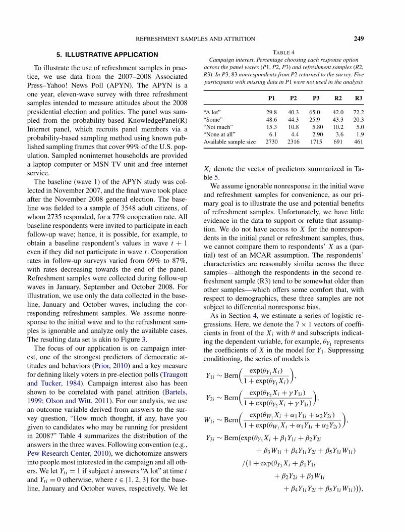
The focus of our application is on campaign inter-est, one of the strongest predictors of democratic at-titudes and behaviors (Prior, 2010) and a key measurefor defining likely voters in pre-election polls (Traugottand Tucker, 1984). Campaign interest also has beenshown to be correlated with panel attrition (Bartels,1999; Olson and Witt, 2011). For our analysis, we usean outcome variable derived from answers to the sur-vey question, “How much thought, if any, have yougiven to candidates who may be running for presidentin 2008?” Table 4 summarizes the distribution of theanswers in the three waves. Following convention (e.g.,Pew Research Center, 2010), we dichotomize answersinto people most interested in the campaign and all oth-ers. We let Yti = 1 if subject i answers “A lot” at time t

and Yti = 0 otherwise, where t ∈ {1,2,3} for the base-line, January and October waves, respectively. We let

TABLE 4Campaign interest. Percentage choosing each response option

across the panel waves (P1, P2, P3) and refreshment samples (R2,R3). In P3, 83 nonrespondents from P2 returned to the survey. Fiveparticipants with missing data in P1 were not used in the analysis

P1 P2 P3 R2 R3

“A lot” 29.8 40.3 65.0 42.0 72.2“Some” 48.6 44.3 25.9 43.3 20.3“Not much” 15.3 10.8 5.80 10.2 5.0“None at all” 6.1 4.4 2.90 3.6 1.9Available sample size 2730 2316 1715 691 461

Xi denote the vector of predictors summarized in Ta-ble 5.

We assume ignorable nonresponse in the initial waveand refreshment samples for convenience, as our pri-mary goal is to illustrate the use and potential benefitsof refreshment samples. Unfortunately, we have littleevidence in the data to support or refute that assump-tion. We do not have access to X for the nonrespon-dents in the initial panel or refreshment samples, thus,we cannot compare them to respondents’ X as a (par-tial) test of an MCAR assumption. The respondents’characteristics are reasonably similar across the threesamples—although the respondents in the second re-freshment sample (R3) tend to be somewhat older thanother samples—which offers some comfort that, withrespect to demographics, these three samples are notsubject to differential nonresponse bias.

As in Section 4, we estimate a series of logistic re-gressions. Here, we denote the 7 × 1 vectors of coeffi-cients in front of the Xi with θ and subscripts indicat-ing the dependent variable, for example, θY1 representsthe coefficients of X in the model for Y1. Suppressingconditioning, the series of models is

Y1i ∼ Bern(

exp(θY1Xi)

1 + exp(θY1Xi)

),

Y2i ∼ Bern(

exp(θY2Xi + γ Y1i )

1 + exp(θY2Xi + γ Y1i )

),

W1i ∼ Bern(

exp(θW1Xi + α1Y1i + α2Y2i )

1 + exp(θW1Xi + α1Y1i + α2Y2i )

),

Y3i ∼ Bern(exp(θY3Xi + β1Y1i + β2Y2i

+ β3W1i + β4Y1iY2i + β5Y1iW1i )

/(1 + exp(θY3Xi + β1Y1i

+ β2Y2i + β3W1i

+ β4Y1iY2i + β5Y1iW1i )))

,

250 Y. DENG ET AL.

TABLE 5Predictors used in all conditional models, denoted as X. Percentage of respondents in each category in initial

panel (P1) and refreshment samples (R2, R3)

Variable Definition P1 R2 R3

AGE1 = 1 for age 30–44, = 0 otherwise 0.28 0.28 0.21AGE2 = 1 for age 45–59, = 0 otherwise 0.32 0.31 0.34AGE3 = 1 for age above 60, = 0 otherwise 0.25 0.28 0.34MALE = 1 for male, = 0 for female 0.45 0.47 0.43COLLEGE = 1 for having college degree, = 0 otherwise 0.30 0.33 0.31BLACK = 1 for African American, = 0 otherwise 0.08 0.07 0.07INT = 1 for everyone (the intercept)

W2i ∼ Bern(exp(θW2Xi + δ1Y1i + δ2Y2i + δ3Y3i

+ δ4W1i + δ5Y1iY2i + δ6Y1iW1i )

/(1 + exp(θW2Xi + δ1Y1i + δ2Y2i

+ δ3Y3i + δ4W1i

+ δ5Y1iY2i + δ6Y1iW1i )))

.

We use noninformative prior distributions on all pa-rameters. We estimate posterior distributions of the pa-rameters using a Metropolis-within-Gibbs algorithm,running the chain for 200,000 iterations and treat-ing the first 50% as burn-in. MCMC diagnostics sug-gested that the chain converged. Running the MCMCfor 200,000 iterations took approximately 3 hours ona standard desktop computer (Intel Core 2 Duo CPU3.00 GHz, 4 GB RAM). We developed the code in Mat-lab without making significant efforts to optimize thecode. Of course, running times could be significantlyfaster with higher-end machines and smarter coding ina language like C++.

The identification conditions include no interactionbetween campaign interest in wave 1 and wave 2 whenpredicting attrition in wave 2, and no interaction be-tween campaign interest in wave 3 (as well as nonre-sponse in wave 2) and other variables when predictingattrition in wave 3. These conditions are impossible tocheck from the sampled data alone, but we cannot thinkof any scientific basis to reject them outright.

Table 6 summarizes the posterior distributions of theregression coefficients in each of the models. Based onthe model for W1, attrition in the second wave is rea-sonably described as missing at random, since the coef-ficient of Y2 in that model is not significantly differentfrom zero. The model for W2 suggests that attrition inwave 3 is not missing at random. The coefficient forY3 indicates that participants who were strongly inter-ested in the election at wave 3 (holding all else con-

stant) were more likely to drop out. Thus, a panel attri-tion correction is needed to avoid making biased infer-ences.

This result contradicts conventional wisdom thatpolitically-interested respondents are less likely to at-trite (Bartels, 1999). The discrepancy could result fromdifferences in the survey design of the APYN studycompared to previous studies with attrition. For exam-ple, the APYN study consisted of 10–15 minute on-line interviews, whereas the ANES panel analyzed byBartels (1999) and Olson and Witt (2011) consisted of90-minute, face-to-face interviews. The lengthy ANESinterviews have been linked to significant panel condi-tioning effects, in which respondents change their at-titudes and behavior as a result of participation in thepanel (Bartels, 1999). In contrast, Kruse et al. (2009)finds few panel conditioning effects in the APYNstudy. More notably, there was a differential incen-tive structure in the APYN study. In later waves ofthe study, reluctant responders (those who took morethan 7 days to respond in earlier waves) received in-creased monetary incentives to encourage their partici-pation. Other panelists and the refreshment sample re-spondents received a standard incentive. Not surpris-ingly, the less interested respondents were more likelyto have received the bonus incentives, potentially in-creasing their retention rate to exceed that of the mostinterested respondents. This possibility raises a broaderquestion about the reasonableness of assuming the ini-tial nonresponse is ignorable, a point we return to inSection 6.

In terms of the campaign interest variables, the ob-served relationships with (Y1, Y2, Y3) are consistentwith previous research (Prior, 2010). Not surprisingly,the strongest predictor of interest in later waves is in-terest in previous waves. Older and college-educatedparticipants are more likely to be interested in the elec-tion. Like other analyses of the 2008 election (Lawless,

REFRESHMENT SAMPLES AND ATTRITION 251

TABLE 6Posterior means and 95% central intervals for coefficients in regressions. Column headers are the dependent variable in the regressions

Variable Y1 Y2 Y3 W1 W2

INT −1.60 −1.77 0.04 1.64 −1.40(−1.94,−1.28) (−2.21,−1.32) (−1.26,1.69) (1.17,2.27) (−2.17,−0.34)

AGE1 0.25 0.27 0.03 −0.08 0.28(−0.12,0.63) (−0.13,0.68) (−0.40,0.47) (−0.52,0.37) (−0.07,0.65)

AGE2 0.75 0.62 0.15 0.24 0.27(0.40,1.10) (0.24,1.02) (−0.28,0.57) (−0.25,0.72) (−0.07,0.64)

AGE3 1.26 0.96 0.88 0.37 0.41(0.91,1.63) (0.57,1.37) (0.41,1.34) (−0.14,0.87) (0.04,0.80)

COLLEGE 0.11 0.53 0.57 0.35 0.58(−0.08,0.31) (0.31,0.76) (0.26,0.86) (0.04,0.69) (0.34,0.84)

MALE −0.05 −0.02 −0.02 0.13 0.08(−0.23,0.13) (−0.22,0.18) (−0.29,0.24) (−0.13,0.39) (−0.14,0.29)

BLACK 0.75 −0.02 0.11 −0.54 −0.12(0.50,1.00) (−0.39,0.35) (−0.40,0.64) (−0.92,−0.14) (−0.47,0.26)

Y1 — 2.49 1.94 0.50 0.88— (2.24,2.73) (0.05,3.79) (−0.28,1.16) (0.20,1.60)

Y2 — — 2.03 −0.58 0.27— — (1.61,2.50) (−1.92,0.89) (−0.13,0.66)

W1 — — −0.42 — 2.47— — (−1.65,0.69) — (2.07,2.85)

Y1Y2 — — −0.37 — −0.07— — (−1.18,0.47) — (−0.62,0.48)

Y1W1 — — −0.52 — −0.62— — (−2.34,1.30) — (−1.18,−0.03)

Y3 — — — — −1.10— — — — (−3.04,−0.12)

2009), and in contrast to many previous election cycles,we do not find a significant gender gap in campaign in-terest.

We next illustrate the P-only approach with multi-ple imputation. We used the posterior draws of param-eters to create m = 500 completed data sets of the orig-inal panel only. We thinned the chains until autocorre-lations of the parameters were near zero to obtain theparameter sets. We then estimated marginal probabil-ities of (Y2, Y3) and a logistic regression for Y3 usingmaximum likelihood on only the 2730 original panelcases, obtaining inferences via Rubin’s (1987) com-bining rules. For comparison, we estimated the samequantities using only the 1632 complete cases, that is,people who completed all three waves.

The estimated marginal probabilities reflect the re-sults in Table 6. There is little difference in P(Y2 = 1)

in the two analyses: the 95% confidence interval is(0.38,0.42) in the complete cases and (0.37,0.46) inthe full panel after multiple imputation. However, thereis a suggestion of attrition bias in P(Y3 = 1). The95% confidence interval is (0.63,0.67) in the complete

cases and (0.65,0.76) in the full panel after multipleimputation. The estimated P(Y3 = 1 | W2 = 0) = 0.78,suggesting that nonrespondents in the third wave weresubstantially more interested in the campaign than re-spondents.

Table 7 displays the point estimates and 95% confi-dence intervals for the regression coefficients for bothanalyses. The results from the two analyses are quitesimilar except for the intercept, which is smaller af-ter adjustment for attrition. The relationship between acollege education and political interest is somewhat at-tenuated after correcting for attrition, although the con-fidence intervals in the two analyses overlap substan-tially. Thus, despite an apparent attrition bias affectingthe marginal distribution of political interest in wave 3,the coefficients for this particular complete-case anal-ysis appear not to be degraded by panel attrition.

Finally, we conclude the analysis with a diagnos-tic check of the three-wave model following the ap-proach outlined in Section 3.3. To do so, we generate500 independent replications of (Y2, Y3) for each of thecells in Figure 3 containing observed responses. We

252 Y. DENG ET AL.

TABLE 7Maximum likelihood estimates and 95% confidence intervals

based for coefficients of predictors of Y3 using m = 500 multipleimputations and only complete cases at final wave

Variable Multiple imputation Complete cases

INT −0.22 (−0.80,0.37) −0.64 (−0.98,−0.31)

AGE1 −0.03 (−0.40,0.34) 0.01 (−0.36,0.37)

AGE2 0.08 (−0.30,0.46) 0.12 (−0.25,0.49)

AGE3 0.74 (0.31,1.16) 0.76 (0.36,1.16)

COLLEGE 0.56 (0.27,0.86) 0.70 (0.43,0.96)

MALE −0.09 (−0.33,0.14) −0.08 (−0.32,0.16)

BLACK 0.07 (−0.38,0.52) 0.05 (−0.43,0.52)

Y1 1.39 (0.87,1.91) 1.45 (0.95,1.94)

Y2 2.00 (1.59,2.40) 2.06 (1.67,2.45)

Y1Y2 −0.33 (−1.08,0.42) −0.36 (−1.12,0.40)

then compare the estimated probabilities for (Y2, Y3)

in the replicated data to the corresponding probabilitiesin the observed data, computing the value of ppp foreach cell. We also estimate the regression from Table 7with the replicated data using only the complete casesin the panel, and compare coefficients from the repli-cated data to those estimated with the complete casesin the panel. As shown in Table 8, the imputation mod-els generate data that are highly compatible with theobserved data in the panel and the refreshment sam-ples on both the conditional probabilities and regres-sion coefficients. Thus, from these diagnostic checkswe do not have evidence of lack of model fit.

6. CONCLUDING REMARKS

The APYN analyses, as well as the simulations, il-lustrate the benefits of refreshment samples for diag-nosing and adjusting for panel attrition bias. At thesame time, it is important to recognize that the ap-proach alone does not address other sources of non-response bias. In particular, we treated nonresponse inwave 1 and the refreshment samples as ignorable. Al-though this simplifying assumption is the usual prac-tice in the attrition correction literature (e.g., Hiranoet al., 1998; Bhattacharya, 2008), it is worth question-ing whether it is defensible in particular settings. Forexample, suppose in the APYN survey that people dis-interested in the campaign chose not to respond to therefreshment samples, for example, because people dis-interested in the campaign were more likely to agreeto take part in a political survey one year out than onemonth out from the election. In such a scenario, themodels would impute too many interested participants

TABLE 8Posterior predictive probabilities (ppp) based on 500 replicateddata sets and various observed-data quantities. Results include

probabilities for cells with observed data and coefficients inregression of Y3 on several predictors estimated with complete

cases in the panel

Quantity Value of ppp

Probabilities observable in original dataPr(Y2 = 0) in the 1st refreshment sample 0.84Pr(Y3 = 0) in the 2nd refreshment sample 0.40Pr(Y2 = 0|W1 = 1) 0.90Pr(Y3 = 0|W1 = 1,W2 = 1) 0.98Pr(Y3 = 0|W1 = 0,W2 = 1) 0.93Pr(Y2 = 0, Y3 = 0|W1 = 1,W2 = 1) 0.98Pr(Y2 = 0, Y3 = 1|W1 = 1,W2 = 1) 0.87Pr(Y2 = 1, Y3 = 0|W1 = 1,W2 = 1) 0.92

Coefficients in regression of Y3 onINT 0.61AGE1 0.72AGE2 0.74AGE3 0.52COLLEGE 0.89MALE 0.76BLACK 0.90Y1 0.89Y2 0.84Y1Y2 0.89

among the panel attriters, leading to bias. Similar is-sues can arise with item nonresponse not due to attri-tion.

We are not aware of any published work in whichnonignorable nonresponse in the initial panel or re-freshment samples is accounted for in inference. Onepotential path forward is to break the nonresponse ad-justments into multiple stages. For example, in stageone the analyst imputes plausible values for the non-respondents in the initial wave and refreshment sam-ple(s) using selection or pattern mixture models de-veloped for cross-sectional data (see Little and Rubin,2002). These form a completed data set except for at-trition and missingness by design, so that we are backin the setting that motivated Sections 3 and 4. In stagetwo, the analyst estimates the appropriate AN modelwith the completed data to perform multiple imputa-tions for attrition (or to use model-based or survey-weighted inference). The analyst can investigate thesensitivity of inferences to multiple assumptions aboutthe nonignorable missingness mechanisms in the ini-tial wave and refreshment samples. This approach isrelated to two-stage multiple imputation (Shen, 2000;Rubin, 2003; Siddique, Harel and Crespi, 2012)

REFRESHMENT SAMPLES AND ATTRITION 253

More generally, refreshment samples need to be rep-resentative of the population of interest to be informa-tive. In many contexts, this requires closed populationsor, at least, populations with characteristics that do notchange over time in unobservable ways. For example,the persistence effect in the APYN multiple imputationanalysis (i.e., people interested in earlier waves remaininterested in later waves) would be attenuated if peoplewho are disinterested in the initial wave and would beso again in a later wave are disproportionately removedfrom the population after the first wave. Major popula-tion composition changes are rare in most short-termnational surveys like the APYN, although this could bemore consequential in panel surveys with a long timehorizon or of specialized populations.

We presented model-based and multiple imputationapproaches to utilizing the information in refreshmentsamples. One also could use approaches based on in-verse probability weighting. We are not aware of anypublished research that thoroughly evaluates the meritsof the various approaches in refreshment sample con-texts. The only comparison that we identified was inNevo (2003)—which weights the complete cases of thepanel so that the moments of the weighted data equalthe moments in the refreshment sample—who brieflymentions towards the end of his article that the resultsfrom the weighting approach and the multiple imputa-tion in Hirano et al. (1998) are similar. We note thatNevo (2003) too has to make identification assump-tions about interaction effects in the selection model.

It is important to emphasize that the combined datado not provide any information about the interactioneffects that we identify as necessary to exclude fromthe models. There is no way around making assump-tions about these effects. As we demonstrated, whenthe assumptions are wrong, the additive nonignorablemodels could generate inaccurate results. This limi-tation plagues model-based, multiple imputation andre-weighting methods. The advantage of including re-freshment samples in data collection is that they allowone to make fewer assumptions about the missing datamechanism than if only the original panel were avail-able. It is relatively straightforward to perform sensi-tivity analyses to this separability assumption in two-wave settings with modest numbers of outcome vari-ables; however, these sensitivity analyses are likely tobe cumbersome when many coefficients are set to zeroin the constraints, as is the case with multiple outcomevariables or waves.

In sum, refreshment samples offer valuable informa-tion that can be used to adjust inferences for nonig-norable attrition or to create multiple imputations for

secondary analysis. We believe that many longitudinaldata sets could benefit from the use of such samples,although further practical development is needed, in-cluding methodology for handling nonignorable unitand item nonresponse in the initial panel and refresh-ment samples, flexible modeling strategies for high-dimensional panel data, efficient methodologies for in-verse probability weighting and thorough comparisonsof them to model-based and multiple imputation ap-proaches, and methods for extending to more complexdesigns like multiple waves between refreshment sam-ples. We hope that this article encourages researchersto work on these issues and data collectors to considersupplementing their longitudinal panels with refresh-ment samples.

ACKNOWLEDGMENTS

Research supported in part by NSF Grant SES-10-61241.

REFERENCES

AHERN, K. and LE BROCQUE, R. (2005). Methodological issuesin the effects of attrition: Simple solutions for social scientists.Field Methods 17 53–69.

BARNARD, J. and MENG, X. L. (1999). Applications of multipleimputation in medical studies: From AIDS to NHANES. Stat.Methods Med. Res. 8 17–36.

BARNARD, J. and RUBIN, D. B. (1999). Small-sample degreesof freedom with multiple imputation. Biometrika 86 948–955.MR1741991

BARTELS, L. (1993). Messages received: The political impact ofmedia exposure. American Political Science Review 88 267–285.

BARTELS, L. (1999). Panel effects in the American National Elec-tion Studies. Political Analysis 8 1–20.

BASIC, E. and RENDTEL, U. (2007). Assessing the bias due tonon-coverage of residential movers in the German Microcen-sus Panel: An evaluation using data from the Socio-EconomicPanel. AStA Adv. Stat. Anal. 91 311–334. MR2405432

BEHR, A., BELLGARDT, E. and RENDTEL, U. (2005). Extentand determinants of panel attrition in the European CommunityHousehold Panel. European Sociological Review 23 81–97.

BHATTACHARYA, D. (2008). Inference in panel data models un-der attrition caused by unobservables. J. Econometrics 144 430–446. MR2436950

BURGETTE, L. F. and REITER, J. P. (2010). Multiple imputationfor missing data via sequential regression trees. Am. J. Epi-demiol. 172 1070–1076.

CHEN, H. Y. and LITTLE, R. (1999). A test of missing completelyat random for generalised estimating equations with missingdata. Biometrika 86 1–13. MR1688067

CHEN, B., YI, G. Y. and COOK, R. J. (2010). Weighted general-ized estimating functions for longitudinal response and covari-ate data that are missing at random. J. Amer. Statist. Assoc. 105336–353. MR2757204

254 Y. DENG ET AL.

CLINTON, J. (2001). Panel bias from attrition and conditioning:A case study of the Knowledge Networks Panel. Unpublishedmanuscript, Vanderbilt Univ. Available at https://my.vanderbilt.edu/joshclinton/files/2011/10/C_WP2001.pdf.

DANIELS, M. J. and HOGAN, J. W. (2008). Missing Data in Lon-gitudinal Studies: Strategies for Bayesian Modeling and Sensi-tivity Analysis. Monographs on Statistics and Applied Probabil-ity 109. Chapman & Hall/CRC, Boca Raton, FL. MR2459796

DAS, M. (2004). Simple estimators for nonparametric panel datamodels with sample attrition. J. Econometrics 120 159–180.MR2047784

DENG, Y. (2012). Modeling missing data in panel studies withmultiple refreshment samples. Master’s thesis, Dept. StatisticalScience, Duke Univ, Durham, NC.

DIGGLE, P. (1989). Testing for random dropouts in repeated mea-surement data. Biometrics 45 1255–1258.

DIGGLE, P. J., HEAGERTY, P. J., LIANG, K.-Y. and ZEGER, S. L.(2002). Analysis of Longitudinal Data, 2nd ed. Oxford Statisti-cal Science Series 25. Oxford Univ. Press, Oxford. MR2049007

DORSETT, R. (2010). Adjusting for nonignorable sample attritionusing survey substitutes identified by propensity score match-ing: An empirical investigation using labour market data. Jour-nal of Official Statistics 26 105–125.

FITZGERALD, J., GOTTSCHALK, P. and MOFFITT, R. (1998). Ananalysis of sample attrition in panel data: The Michigan PanelStudy of Income Dynamics. Journal of Human Resources 33251–299.

FITZMAURICE, G. M., LAIRD, N. M. and WARE, J. H.(2004). Applied Longitudinal Analysis. Wiley, Hoboken, NJ.MR2063401

FRICK, J. R., GOEBEL, J., SCHECHTMAN, E., WAGNER, G. G.and YITZHAKI, S. (2006). Using analysis of Gini (ANOGI) fordetecting whether two subsamples represent the same universe.Sociol. Methods Res. 34 427–468. MR2247101

GELMAN, A. (2007). Struggles with survey weighting and regres-sion modeling. Statist. Sci. 22 153–164. MR2408951

GELMAN, A., MENG, X.-L. and STERN, H. (1996). Posterior pre-dictive assessment of model fitness via realized discrepancies(with discussion). Statist. Sinica 6 733–807. MR1422404

HAUSMAN, J. and WISE, D. (1979). Attrition bias in experimen-tal and panel data: The Gary income maintenance experiment.Econometrica 47 455–473.

HE, Y., ZASLAVSKY, A. M., LANDRUM, M. B., HARRING-TON, D. P. and CATALANO, P. (2010). Multiple imputation ina large-scale complex survey: A practical guide. Stat. MethodsMed. Res. 19 653–670. MR2744515

HEDEKER, D. and GIBBONS, R. D. (2006). Longitudinal DataAnalysis. Wiley, Hoboken, NJ. MR2284230

HEERINGA, S. (1997). Russia longitudinal monitoring survey sam-ple attrition, replenishment, and weighting: Rounds V–VII.Univ. Michigan Institute for Social Research.

HENDERSON, M., HILLYGUS, D. and TOMPSON, T. (2010).“Sour grapes” or rational voting? Voter decision making amongthwarted primary voters in 2008. Public Opinion Quarterly 74499–529.

HIRANO, K., IMBENS, G., RIDDER, G. and RUBIN, D. (1998).Combining panel data sets with attrition and refreshment sam-ples. NBER Working Paper 230.

HIRANO, K., IMBENS, G. W., RIDDER, G. and RUBIN, D. B.(2001). Combining panel data sets with attrition and refresh-ment samples. Econometrica 69 1645–1659. MR1865224

HONAKER, J. and KING, G. (2010). What to do about missingvalues in time-series cross-section data. American Journal ofPolitical Science 54 561–581.

JELICIC, H., PHELPS, E. and LERNER, R. M. (2009). Use of miss-ing data methods in longitudinal studies: The persistence of badpractices in developmental psychology. Dev. Psychol. 45 1195–1199.

KALTON, G. and KASPRZYK, D. (1986). The treatment of missingsurvey data. Survey Methodology 12 1–16.

KENWARD, M. G. (1998). Selection models for repeated measure-ments with non-random dropout: An illustration of sensitivity.Stat. Med. 17 2723–2732.

KENWARD, M. G., MOLENBERGHS, G. and THIJS, H.(2003). Pattern-mixture models with proper time dependence.Biometrika 90 53–71. MR1966550

KISH, L. and HESS, I. (1959). A “replacement” procedure for re-ducing the bias of nonresponse. Amer. Statist. 13 17–19.

KRISTMAN, V., MANNO, M. and COTE, P. (2005). Methods toaccount for attrition in longitudinal data: Do they work? A sim-ulation study. European Journal of Epidemiology 20 657–662.

KRUSE, Y., CALLEGARO, M., DENNIS, J., SUBIAS, S.,LAWRENCE, M., DISOGRA, C. and TOMPSON, T. (2009).Panel conditioning and attrition in the AP-Yahoo! News Elec-tion Panel Study. In 64th Conference of the American Associa-tion for Public Opinion Research (AAPOR), Hollywood, FL.

LAWLESS, J. (2009). Sexism and gender bias in election 2008:A more complex path for women in politics. Politics Gender5 70–80.

LI, K. H., RAGHUNATHAN, T. E. and RUBIN, D. B. (1991).Large-sample significance levels from multiply imputed datausing moment-based statistics and an F reference distribution.J. Amer. Statist. Assoc. 86 1065–1073. MR1146352

LI, K. H., MENG, X.-L., RAGHUNATHAN, T. E. and RU-BIN, D. B. (1991). Significance levels from repeated p-values with multiply-imputed data. Statist. Sinica 1 65–92.MR1101316

LIN, H., MCCULLOCH, C. E. and ROSENHECK, R. A. (2004).Latent pattern mixture models for informative intermittentmissing data in longitudinal studies. Biometrics 60 295–305.MR2066263

LIN, I. and SCHAEFFER, N. C. (1995). Using survey partici-pants to estimate the impact of nonparticipation. Public OpinionQuarterly 59 236–258.

LITTLE, R. J. A. (1993). Pattern-mixture models for multivariateincomplete data. J. Amer. Statist. Assoc. 88 125–134.

LITTLE, R. J. A. and RUBIN, D. B. (2002). Statistical Analysiswith Missing Data, 2nd ed. Wiley, Hoboken, NJ. MR1925014

LOHR, S. (1998). Sampling: Design and Analysis. Cole PublishingCompany, London.

LYNN, P. (2009). Methodology of Longitudinal Surveys. Wiley,Chichester, UK.

MENG, X.-L. (1994). Posterior predictive p-values. Ann. Statist.22 1142–1160. MR1311969

MENG, X.-L. and RUBIN, D. B. (1992). Performing likelihoodratio tests with multiply-imputed data sets. Biometrika 79 103–111. MR1158520

MOLENBERGHS, G., BEUNCKENS, C., SOTTO, C. and KEN-WARD, M. G. (2008). Every missingness not at random modelhas a missingness at random counterpart with equal fit. J. R.Stat. Soc. Ser. B Stat. Methodol. 70 371–388. MR2424758

REFRESHMENT SAMPLES AND ATTRITION 255

NEVO, A. (2003). Using weights to adjust for sample selectionwhen auxiliary information is available. J. Bus. Econom. Statist.21 43–52. MR1950376

OLSEN, R. (2005). The problem of respondent attrition: Surveymethodology is key. Monthly Labor Review 128 63–71.

OLSON, K. and WITT, L. (2011). Are we keeping the people whoused to stay? Changes in correlates of panel survey attrition overtime. Social Science Research 40 1037–1050.

PACKER, M., COLUCCI, W., SACKNER-BERNSTEIN, J.,LIANG, C., GOLDSCHER, D., FREEMAN, I., KUKIN, M.,KINHAL, V., UDELSON, J., KLAPHOLZ, M. et al. (1996).Double-blind, placebo-controlled study of the effects ofcarvedilol in patients with moderate to severe heart failure: ThePRECISE trial. Circulation 94 2800–2806.

PASEK, J., TAHK, A., LELKES, Y., KROSNICK, J., PAYNE, B.,AKHTAR, O. and TOMPSON, T. (2009). Determinants ofturnout and candidate choice in the 2008 US Presidential elec-tion: Illuminating the impact of racial prejudice and other con-siderations. Public Opinion Quarterly 73 943–994.

PEW RESEARCH CENTER (2010). Four years later republicansfaring better with men, whites, independents and seniors(press release). Available at http://www.people-press.org/files/legacy-pdf/643.pdf.

PRIOR, M. (2010). You’ve either got it or you don’t? The stabilityof political interest over the life cycle. The Journal of Politics72 747–766.

QU, A. and SONG, P. X. K. (2002). Testing ignorable missing-ness in estimating equation approaches for longitudinal data.Biometrika 89 841–850. MR1946514

QU, A., YI, G. Y., SONG, P. X. K. and WANG, P. (2011). Assess-ing the validity of weighted generalized estimating equations.Biometrika 98 215–224. MR2804221

RAGHUNATHAN, T. E., LEPKOWSKI, J. M., VAN HOEWYK, J.and SOLENBERGER, P. (2001). A multivariate technique formultiply imputing missing values using a series of regressionmodels. Survey Methodology 27 85–96.

REITER, J. P. (2007). Small-sample degrees of freedom for multi-component significance tests for multiple imputation for miss-ing data. Biometrika 94 502–508. MR2380575

REITER, J. P. (2008). Multiple imputation when records used forimputation are not used or disseminated for analysis. Biometrika95 933–946. MR2461221

REITER, J. P. and RAGHUNATHAN, T. E. (2007). The multipleadaptations of multiple imputation. J. Amer. Statist. Assoc. 1021462–1471. MR2372542

RIDDER, G. (1992). An empirical evaluation of some models fornon-random attrition in panel data. Structural Change and Eco-nomic Dynamics 3 337–355.

ROBINS, J. M. and ROTNITZKY, A. (1995). Semiparametric ef-ficiency in multivariate regression models with missing data.J. Amer. Statist. Assoc. 90 122–129. MR1325119

ROBINS, J. M., ROTNITZKY, A. and ZHAO, L. P. (1995). Analysisof semiparametric regression models for repeated outcomes inthe presence of missing data. J. Amer. Statist. Assoc. 90 106–121. MR1325118

ROTNITZKY, A., ROBINS, J. M. and SCHARFSTEIN, D. O.(1998). Semiparametric regression for repeated outcomes withnonignorable nonresponse. J. Amer. Statist. Assoc. 93 1321–1339. MR1666631

ROY, J. (2003). Modeling longitudinal data with nonignorabledropouts using a latent dropout class model. Biometrics 59 829–836. MR2025106

ROY, J. and DANIELS, M. J. (2008). A general class of patternmixture models for nonignorable dropout with many possibledropout times. Biometrics 64 538–545, 668. MR2432424

RUBIN, D. B. (1976). Inference and missing data (with discus-sion). Biometrika 63 581–592. MR0455196

RUBIN, D. B. (1987). Multiple Imputation for Nonresponse in Sur-veys. Wiley, New York. MR0899519

RUBIN, D. B. (1996). Multiple imputation after 18+ years.J. Amer. Statist. Assoc. 91 473–489.

RUBIN, D. B. (2003). Nested multiple imputation of NMESvia partially incompatible MCMC. Stat. Neerl. 57 3–18.MR2055518

RUBIN, D. and ZANUTTO, E. (2001). Using matched substitutes toadjust for nonignorable nonresponse through multiple imputa-tions. In Survey Nonresponse (R. Groves, D. Dillman, R. Littleand J. Eltinge, eds.) 389–402. Wiley, New York.

SCHAFER, J. L. (1997). Analysis of Incomplete Multivariate Data.Monographs on Statistics and Applied Probability 72. Chapman& Hall, London. MR1692799

SCHARFSTEIN, D. O., ROTNITZKY, A. and ROBINS, J. M.(1999). Adjusting for nonignorable drop-out using semipara-metric nonresponse models. J. Amer. Statist. Assoc. 94 1096–1120.

SEMYKINA, A. and WOOLDRIDGE, J. M. (2010). Estimatingpanel data models in the presence of endogeneity and selection.J. Econometrics 157 375–380. MR2661609

SHEN, Z. (2000). Nested multiple imputation. Ph.D. thesis, Dept.Statistics, Harvard Univ. MR2700720

SIDDIQUE, J., HAREL, O. and CRESPI, C. M. (2012). Addressingmissing data mechanism uncertainty using multiple imputation:Application to a longitudinal clinical trial. Ann. Appl. Stat. 61814–1837.

SIDDIQUI, O., FLAY, B. and HU, F. (1996). Factors affecting at-trition in a longitudinal smoking prevention study. PreventiveMedicine 25 554–560.

THOMPSON, M., FONG, G., HAMMOND, D., BOUDREAU, C.,DRIEZEN, P., HYLAND, A., BORLAND, R., CUMMINGS, K.,HASTINGS, G., SIAHPUSH, M. et al. (2006). Methods of the In-ternational Tobacco Control (ITC) four country survey. TobaccoControl 15 Suppl. 3.

TRAUGOTT, M. and TUCKER, C. (1984). Strategies for predictingwhether a citizen will vote and estimation of electoral outcomes.Public Opinion Quarterly 48 330–343.

VAN BUUREN, S. and OUDSHOORN, C. (1999). Flexible multi-variate imputation by MICE. Technical Report TNO/VGZ/PG99.054, TNO Preventie en Gezondheid, Leiden.

VANDECASTEELE, L. and DEBELS, A. (2007). Attrition in paneldata: The effectiveness of weighting. European SociologicalReview 23 81–97.

VEHOVAR, V. (1999). Field substitution and unit nonresponse.Journal of Official Statistics 15 335–350.

VELLA, F. and VERBEEK, M. (1999). Two-step estimation ofpanel data models with censored endogenous variables and se-lection bias. J. Econometrics 90 239–263.

VERBEKE, G. and MOLENBERGHS, G. (2000). Linear Mixed Ef-fects Models for Longitudinal Data. Springer, Berlin.

WAWRO, G. (2002). Estimating dynamic panel data models in po-litical science. Political Analysis 10 25–48.

256 Y. DENG ET AL.

WISSEN, L. and MEURS, H. (1989). The Dutch mobility panel:Experiences and evaluation. Transportation 16 99–119.

WOOLDRIDGE, J. M. (2005). Simple solutions to the initial con-ditions problem in dynamic, nonlinear panel data models withunobserved heterogeneity. J. Appl. Econometrics 20 39–54.MR2138202

ZABEL, J. (1998). An analysis of attrition in the Panel Study of In-come Dynamics and the Survey of Income and Program Partic-ipation with an application to a model of labor market behavior.Journal of Human Resources 33 479–506.