survey attrition and attrition bias in young lives - gov.uk · survey attrition and attrition bias...

YOUNG LIVES TECHNICAL NOTE NO. 5

Survey Attrition and Attrition Bias inYoung Lives

Ingo Outes-Leon

Stefan Dercon

March 2008

SURVEY ATTRITION AND ATTRITION BIAS IN YOUNG LIVES

1

Contents Executive summary 2

1. Introduction 8

2. Attrition bias: framework and literature 9

3. Young Lives 13 3.1 Attrition rates 14 3.2 Patterns of non-random attrition 15

4. Testing for attrition bias 17 4.1 Models of child anthropometrics 18 4.2 Models of school enrolment 20

5. Conclusion 21

References 22

Appendix A 24

Attrition in selected Longitudinal Countries 24

Appendix B 25

Non-random Attrition: Variable Means 25

Appendix C 30

Attrition Probit Regressions 30

Appendix D 34

BGLW Test Regressions 34


2

Executive summary Longitudinal studies, such as the Young Lives study of childhood poverty, help us to analyse

welfare dynamics in ways that are not possible using time-series or cross-sectional samples.

However, analysis based on panel datasets can be heavily compromised by sample attrition.

On the one hand, the number of respondents who do not participate in each round of data

collection (wave non-response) will inevitably cumulate over time, resulting in falling sample

sizes, which will undermine the precision of any research undertaken using such samples.

On the other hand, unless it is random, attrition might lead to biased inferences. Analysts

often presuppose that attrition is correlated with observable characteristics such as

household education, health or economic well-being, resulting in samples that include only a

selected group of households. However, even if that is the case, non-random attrition does

not necessarily lead to attrition bias. Attrition bias is model-specific and, as previous studies

have shown, biases might be absent even if attrition rates are high.

We investigate the incidence and potential bias arising from attrition in Young Lives following

the completion of the second round of data collection. Young Lives is a study concerned with

analysing childhood poverty in four countries, Ethiopia, India, Vietnam and Peru. The study,

which measures a range of child, household, and household-member characteristics , is

following two cohorts of children in each country over 15 years – a younger cohort of 2,000

children who were born in 2001 to 2002 (i.e. aged 6 to 18 months when first surveyed) and

1,000 older children born in 1994-95 (i.e. aged 7.5 to 8.5 at the start of the survey).

Sample attrition is particularly concerning in the context of a longitudinal study such as Young

Lives where cohort sample sizes are modest and individuals are tracked over a relatively

long period of time. This paper seeks to:

• document the rates of attrition of the Young Lives study following completion of the

second round of data collection;

• investigate the extent to which sample attrition is non-random;

• analyse whether non-random attrition in the Young Lives sample might lead to attrition

bias.

Attrition bias and methodology

Attrition bias arises when sample attrition is non-random and the variables affecting attrition

might be correlated with the outcome variable of interest such as household education,

health or economic well-being. More formally, attrition bias will occur if the error term in the

equation of interest is correlated with the error term in the selection or attrition equation. In

this respect, attrition bias is model specific as the correlation between the error terms will

depend on the precise specification of the model.1

In analysing attrition bias, we follow the framework set out in Fitzgerald, Gottschalk and

Moffitt (1998). In their seminal study on attrition bias in the US Panel Study of Income

Dynamics (PSID) sample, they distinguish between attrition on unobservables and

observables, and provide a series of tests designed to assess incidence of attrition bias.

In this paper, we focus on attrition on observables. We assess attrition bias on two types of

child welfare models. For the younger cohort we estimate models of child health as

1 J. Wooldridge (2002) Econometric Analysis of Cross Section and Panel Data, Cambridge MA: MIT Press


3

measured by anthropometric height-for-age and weight-for-height z-scores. For the older

cohort, we estimate a model of school enrolment at the age of eight.

In assessing attrition bias, we use two complementary types of tests. First, we carry out

attrition probit tests proposed by Fitzgerald, Gottschalk and Moffitt (1998) (FGM tests).

Second, we perform the tests first suggested by Becketti, Gould, Lillard and Welch (1988)

(known as the BGLW test). As pointed out by Fitzgerald, Gottschalk and Moffitt (1998), both

set of tests are related and tend to provide broadly consistent results.

Main evidence

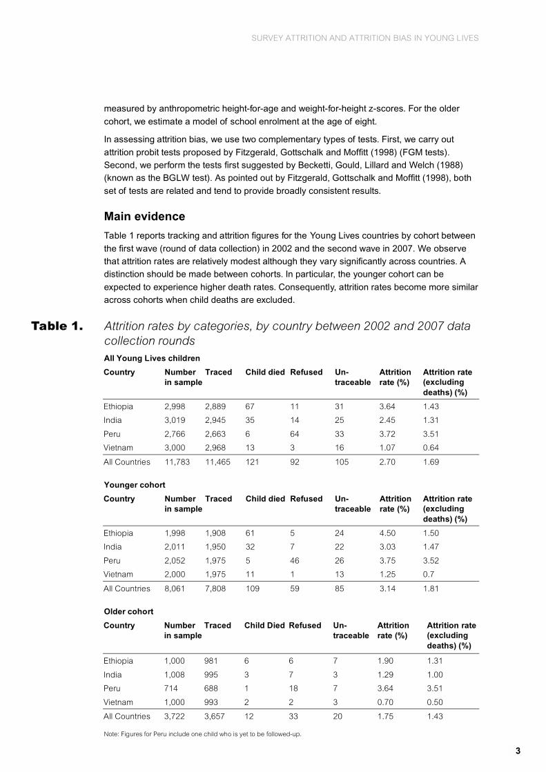
Table 1 reports tracking and attrition figures for the Young Lives countries by cohort between

the first wave (round of data collection) in 2002 and the second wave in 2007. We observe

that attrition rates are relatively modest although they vary significantly across countries. A

distinction should be made between cohorts. In particular, the younger cohort can be

expected to experience higher death rates. Consequently, attrition rates become more similar

across cohorts when child deaths are excluded.

Table 1. Attrition rates by categories, by country between 2002 and 2007 data collection rounds

All Young Lives children

Country Number

in sample

Traced Child died Refused

Un-

traceable

Attrition

rate (%)

Attrition rate (excluding

deaths) (%)

Ethiopia 2,998 2,889 67 11 31 3.64 1.43

India 3,019 2,945 35 14 25 2.45 1.31

Peru 2,766 2,663 6 64 33 3.72 3.51

Vietnam 3,000 2,968 13 3 16 1.07 0.64

All Countries 11,783 11,465 121 92 105 2.70 1.69

Younger cohort

Country Number

in sample

Traced Child died Refused Un-

traceable

Attrition

rate (%)


deaths) (%)

Ethiopia 1,998 1,908 61 5 24 4.50 1.50

India 2,011 1,950 32 7 22 3.03 1.47

Peru 2,052 1,975 5 46 26 3.75 3.52

Vietnam 2,000 1,975 11 1 13 1.25 0.7

All Countries 8,061 7,808 109 59 85 3.14 1.81

Older cohort

Country Number

in sample

Traced Child Died Refused Un-

traceable

Attrition

rate (%)


deaths) (%)

Ethiopia 1,000 981 6 6 7 1.90 1.31

India 1,008 995 3 7 3 1.29 1.00

Peru 714 688 1 18 7 3.64 3.51

Vietnam 1,000 993 2 2 3 0.70 0.50

All Countries 3,722 3,657 12 33 20 1.75 1.43

Note: Figures for Peru include one child who is yet to be followed-up.


4

We find that attrition rates in Young Lives are not only small in absolute terms, but are also

low when compared with attrition rates for other longitudinal studies in less developed

countries. Table 2 reports annualised attrition rates for the Young Lives sample and a

number of longitudinal studies. We note that although the Young Lives Peru sample has

higher attrition rates than other Young Lives countries, even these remain very modest

compared to other longitudinal studies.

Table 2. Comparison of attrition rates: Young Lives and other longitudinal studies, annualised attrition rates2

Longitudinal study

(with start date)

Level of

observation

Attrition rate per

annum (%)

Attrition rate per annum (%)

(excluding

deaths)

Description

Young Lives - 2002, All countries

Individual 0.50 0.30 1 follow-up after 4 years

Young Lives - 2002, Peru only Individual 0.74 0.72 1 follow-up after 4 years

KIDS, South Africa - 1993 Household 3.40 3.40 1 follow-up after a 5 year interval

Proyecto Integral de Desarrollo Infantil (PIDI),

Bolivia - 1996,

Individual 19.40 1 follow-up after a 2 year interval

Kenyan Ideational Change Survey (KICS), Kenya – 1994

Household 23.20 1 follow-up after a 2 year interval

Kagera Health and Development Survey (KHDS),

Tanzania – 1991

Household 0.88 0.70 4 rounds of follow-up in 4-year period

Kagera Health and Development Survey (KHDS),

Tanzania – 1994

Individual 2.85 1.60 1 follow-up after 10-year interval

Kagera Health and Development Survey (KHDS), Tanzania – 1994, children

below 10 years

Individual 2.29 1.50 1 follow-up after 10-year interval

Birth to Twenty (BT20), South Africa - 1990

Individual 1.90 1.80 16 years of follow-up, up to 2006

IFORD Yaounde Survey, Cameroon – 1978

Individual 22.50 18.70 7 rounds of follow-up within 2 years

Pelatos Birth Cohort, Brazil, 1982-1986

Individual 5.30 4.20 2 follow-ups of entire sample within 4 years in

1984 and 1986.

Cebu Longitudinal Health and Nutrition Survey (CLHNS),

Philippines - 1983

Individual 2.60 11 year study, 14 rounds in first 2 years, 2 others at

varying intervals

Source: Young Lives data; various studies and own calculations

We investigate non-random attrition by searching for patterns in outcome variables and

household characteristics of attriting households. In Figure 1, we plot kernel densities for the

wealth index for the younger cohort for all countries. Panel A shows that attriting households

2 Rates per annum follow the formula suggested by Alderman et al. (2000) – (1-(1- q))/ . Where q and respectively stand for

attrition rate and year covered by the panel. See Appendix A to the main text of this report for details of sources.


5

have on average a lower wealth index than non-attriting households. A more complex picture

appears when attriting households are split between those where a child has died or those

who refused to participate in the second round of data collection or were untraceable. Here

we find that ‘child deaths’ are correlated with lower wealth index, while households that

refused or were untraceable are correlated with higher values of the wealth index. Further

analysis indicates that, in general, attrition is an urban phenomenon. When split by category,

we find that child deaths mostly occur in rural areas, while untraceable households are

located in urban areas.

Figure 1. Wealth index kernel densities by attrition status (Panel A) and attrition categories (Panel B). All countries, younger cohort only

Panel A Panel B

0

.5

1

1.5

y

0 .2 .4 .6 .8 1

Wealth Index

Non-Attriting Attriting

0

.5

1

1.5

2

2.5

y

0 .2 .4 .6 .8 1

Wealth Index

Non-Attriting Child Death

Refused/Untraceable

More systematically, we compute means of outcome and predetermined variables for the

non-attriting and attriting households, as well as by attrition category. We find that in general,

attriting households tend to have fewer assets, have poorer access to services and utilities

and are less educated, while at the same time their children have poorer health and are less

likely to attend school. These patterns of non-random attrition are particularly strong for

Ethiopia and India, but less so for Peru and Vietnam. As indicated in Figure 1, these

averages hide substantial variation between different types of attriting households. However,

differences in variable means across attrition type, although in some cases substantial, are

not always statistically significant. In summary, we find substantial evidence of non-random

attrition across most countries, although few variables other than urban/rural location and

ethnic background appear to correlate systematically with attrition.

The presence of non-random attrition does not necessarily imply attrition bias. In fact, the

results from probit and BGLW tests provide only very limited evidence of attrition bias.

Furthermore, the R-Square values in the probit regressions provide an indication of the

proportion of attrition that can explained with a full set of child and household characteristics

and the lagged endogenous variable. We find that across different models and countries, the

fitted models explain less than ten per cent of the observed attrition. In other words, even if it

follows some non-random patterns, attrition remains overwhelmingly a random phenomenon.


6

Table 3. Attrition probits, predicting likelihood of attrition, by country and dependent variable (younger cohort only)

Predicting likelihood of attrition Likelihood of attrition

(excluding deaths)

Country Variables

(1) (2) (3) (4) (5)

Ethiopia Height-for-age Coef -0.1129 -0.0969 -0.0716

P-Value 0.001 *** 0.0080 *** 0.2690

Weight-for-height Coef -0.0984 -0.0846 0.1482

P-Value 0.022 ** 0.0560 * 0.0650 *

India Height-for-age Coef -0.0268 -0.0265 -0.0320

P-Value 0.523 0.5280 0.6420


P-Value 0.833 0.8390 0.4610

Peru Height-for-age Coef 0.0232 0.0215 0.0340

P-Value 0.615 0.6430 0.4760


P-Value 0.913 0.6530 0.8150

Vietnam Height-for-age Coef -0.1433 -0.1068 -0.0141

P-Value 0.161 0.3160 0.9230

Weight-for-height Coef -0.1087 -0.0812 -0.0697

P-Value 0.363 0.5060 0.6800

Note: All regressions include as controls household predetermined variables (including information on household head age and

education, household size, household asset holdings, child vaccination and sibling information), as well as caste/ethnic group

dummies. Figures highlighted with (***), (**) and (*) indicate significance at one, five and ten per cent level respectively.

Table 3 reports the results for the attrition probit tests for dependent variables height-for-age

and weight-for-height z-scores. Reported are only figures for the lagged endogenous

variables. Statistical significance of the coefficients for these variables indicates that attrition

bias might be present when modelling child anthropometrics. The table shows that no

evidence of such attrition bias is found, except in Ethiopia where we find that child deaths,

linked to poor child anthropometrics, could lead to biased inferences when fitting child

anthropometric models.

Evidence from the BGLW tests generally supports the findings from the attrition probit tests.

When fitting determinants of outcome variable models, the impact of predetermined variables

on the dependent variables for the full sample and non-attriting sample are statistically

similar. This is true when coefficients are tested both individually and jointly. Moreover, in

spite of the earlier findings, BGLW tests provide no evidence of significant biases in child

anthropometrics in Ethiopia. We interpret this mixed evidence, as a warning for the potential

for biases due to non-random attrition, which at the moment remain weak thanks to modest

rates of attrition.

Conclusion

Although they range widely across countries and attrition category, we find that Young Lives

attrition rates are small in absolute terms. Furthermore, attrition rates are modest when

compared with other longitudinal studies in developing countries. In fact, in all study countries

Young Lives has attrition rates lower than any of the comparison studies.


7

Second, our analysis indicates that attrition is to some extent non-random. In particular, we

find that attrition is primarily an urban phenomenon and that attriting households tend to be

poorer and less educated than non-attriting households.

Third, in spite of non-random attrition we find very limited evidence of attrition bias when

tested on child anthropometric and school enrolment models. On the one hand, very low R-

Squares in the attrition probit models indicate that attrition remains overwhelmingly a random

phenomenon. On the other hand, attrition probit and BGLW tests suggest that attrition on

observables is unlikely to lead to significant biases. Further, limited evidence of attrition bias

found in Ethiopia using attrition probit tests are not corroborated by the BGLW tests;

indicating that, although uncovered patterns of non-random attrition could lead to biases,

modest rates of attrition ensure that attrition bias remains very weak.

In summary, our detailed analysis of the attrition bias of the Young Lives sample strongly

indicates that current attrition is highly unlikely to bias research inferences. However, some

weak evidence of bias alerts us to the importance of ensuring that we continue to track the

children between survey rounds to maintain our current low rates of attrition and not

exacerbate the uncovered non-random patterns of attrition we have noticed to date.


8

1. Introduction Longitudinal studies, such as the Young Lives study of childhood poverty, help us to analyse

welfare dynamics in ways that are not possible using time-series or cross-sectional samples.

However, analysis based on panel datasets can be compromised by sample attrition. On the

one hand, wave non-response (the number of participants who do not respond in each round

of data collection) will inevitably cumulate, resulting in falling sample sizes over time. This will

undermine the precision of any research undertaken using such samples. On the other hand,

unless it is random, survey attrition might lead to biased inferences based on non-attriting

samples. Analysts often presuppose that attrition is correlated with observable characteristics

such as household education, health or economic well-being, resulting in samples that

include only a selected group of households. However, even if that is the case, non-random

attrition does not necessarily lead to attrition bias. Statistical theory suggests that attrition

bias is model specific, and, as previous non-response and attrition studies have shown,

biases mayt be absent even if attrition rates are high.

In this paper, we investigate the incidence and potential bias arising from attrition in the

Young Lives study following the conclusion of the second round of data collection in 2007.

Young Lives is concerned with analysing childhood poverty dynamics in four countries –

Ethiopia, India, Vietnam and Peru. Country surveys initiated in 2002 are following two cohorts

of children, 2,000 one-year olds and 1,000 seven-year olds in each country over a period of

15 years and measure a range of child, household and household-member characteristics.

Sample attrition is particularly concerning for a study such as Young Lives, where cohort

sample sizes are modest and individuals are tracked over a relatively long time. This paper

has three purposes: first, to document the rates of attrition in Young Lives between the 2002

baseline survey and the second round of data collection in 2006/77; second, to investigate

the extent to which sample attrition might be non-random; and finally, to analyse whether

non-random attrition might lead to biased inferences.

In our analysis we follow Fitzgerald, Gottschalk and Moffitt’s seminal work (1998) on attrition

in the US longitudinal Panel Study of Income Dynamics (PSID). First, we uncover any

patterns of non-random attrition by comparing first round profiles between those households

that remained in the sample and those that eventually attrited. Second, we analyse whether

attrition on observables could lead to biased inferences in the Young Lives sample. We test

for attrition bias in the context of two common child welfare models – child anthropometrics

and school enrolment – using two complementary types of tests, the attrition probit tests and

the tests first suggested by Becketti, Gould, Lillard and Welch (1998) (BGLW tests).

Our analysis indicates that while varying significantly across the four Young Lives countries,

attrition rates are very modest. In fact, to the best of our knowledge, Young Lives attrition rates

are the lowest ever reported in the longitudinal studies literature. Further, we find attrition to be

correlated with some observable household and child characteristics, suggesting that patterns

of attrition might be non-random. Finally, in spite of non-random attrition, we find very limited

evidence of attrition bias when tested on child anthropometric and school enrolment models.

On the one hand, very low R-Squares from the probit models indicate that attrition remains

overwhelmingly random. On the other hand, both attrition bias tests reject the existence of

significant biases in the Young Lives sample. In particular, the limited evidence of attrition bias

found using attrition probit tests are not corroborated by the BGLW tests. This indicates that,

although the patterns of non-random attrition we uncovered could potentially lead to biases,

the low rates of attrition ensure that attrition bias remains weak.


9

The remainder of this paper is structured as follows. Section 2 sets out the appropriate

theoretical framework in which attrition should be analysed and provides a brief summary of

the available literature. Section 3 introduces the Young Lives study and describes the

sampling and follow-up methodologies applied. Section 4 documents the Young Lives

attrition rates and analyses the extent to which attrition might be non-random. Section 5

presents the results from the tests on attrition bias, and, finally, section 6 concludes.

2. Attrition bias: framework and literature In their work, Fitzgerald, Gottschalk and Moffitt (1998) develop a theoretical framework for

the analysis of attrition bias, developing a typology whereby attrition on unobservables and

observables can be distinguished. While both types of attrition do not necessarily lead to

biased inferences, when they do it is attrition on observables that is more easily addressed.

Fitzgerald, Gottschalk and Moffitt proposed a series of statistical tests that help determine

whether attrition on observables is likely to lead to biased inferences. They suggested a

Weighted Least Square (WLS) estimation methodology to correct for the potential biases.

Attrition bias can be analysed within a selection model:

(1) y = b0 + b1x + e, y observed if A = 1

(2) A* = a0 + a1x + v

Equation (1) represents the model of interest, whereby the outcome variable (y) is only

observable for the sample of selected households. Equation (2) is a selection model that

determines the likelihood of an observation being observable in the main equation. Latent

index A* is not measurable in practice, but we only observe whether a household has been

selected or not, A = 1 if A* < 0 and A = 0 if A* > 0. Coefficient estimates of model (1) will be

biased due to sample selection if the error terms e and v are correlated. Intuitively this will be

the case when a variable, other than x, affects both selection to and the outcome variable of

the model. It also means that non-random selection does not necessarily lead to biased

estimates. Treating y as an outcome variable from the second period of a longitudinal sample

and equation (2) as an attrition model, we have the equivalent result for attrition bias in a

panel data context (see Maluccio 2000).

The framework presented here makes it particularly clear that attrition bias is model specific.

That is, whether non-random selection is correlated with e depends on the precise model

estimated.

Fitzgerald, Gottschalk and Moffitt build upon this model to distinguish between attrition on

observables and unobservables. Rewriting equation (2) as

(3) A* = d0 + d1x + d2z + u

Selection on observables occurs if z is not independent of e|x but u is independent of e|x. As

the name suggests, selection on observables indicates that all variables that might affect

both the selection equation and the main equation are observable. Stated alternatively,

selection on observables occurs if

(4) Pr(A=0|y, x, z) = Pr(A=0|x, z)


10

Selection on unobservables, on the other hand, occurs if z is independent of e|x but u is not

independent of e|x. That is, equation (4) does not hold and the attrition function cannot be

reduced from Pr(A=0|y, x, z).3 This will be the case if a number of unobserved variables, such

as individual motivation or household entrepreneurship, affect both selection into the model

and the outcome variable of interest.

Under attrition on unobservables, unbiased estimation crucially relies on the existence of a

set of variables z, which affects attrition but does not affect the outcome variable. That is, z

should not be part of x. This is the basis for the widely used sample selection model

estimators (Heckman 1976; Hausman and Wise 1979). However, meeting such exclusionary

restrictions in the context of attrition is more complicated than in other cases, since there are

fewer variables that affect attrition but do not credibly affect the outcome variable. To correct

for this bias, it has been suggested to use data on interviewers and the interviewing process

(see Fitzgerald, Gottschalk and Moffitt 1998; and Zabel 1998).4 However, this route is not

available to us, as no information on the interview process is collected by Young Lives except

in Peru.5

Under attrition on observables, we can address attrition bias, without the need to resort to

exclusionary restricts. If there is selection on observables, the critical variable is z, a variable

which affects the likelihood of attrition but is also related to the density of y conditional on x.

In other words, z is endogenous to the outcome variable, y. Good candidates for z are lagged

values of y, y(-1), as long as they affect attrition but don’t belong in the main equation.6

It is possible to exploit the properties of the variable z to design tests on the existence of

biases due to attrition on observables. Sufficient conditions for the absence of this type of

attrition bias are either (a) z does not affect the likelihood of attrition, A, or (b) z is

independent of y conditional on x. Based on these conditions, Fitzgerald, Gottschalk and

Moffitt suggest the following tests.

First, attrition probit tests rely on the first condition. In this type of test, probit regressions

predicting attrition, A, are fitted including a number of predetermined variables, x, plus a

candidate variable z, typically a lagged dependent variable. Evidence that the z variable has

a significant impact on the likelihood of attrition would indicate that we might encounter

significant attrition bias when modelling variable y.

Further, the R-Square values of the attrition probit regressions provide additional insight into

attrition bias. R-Square values can be interpreted as an estimate of the proportion of attrition

which is non-random - explained by predetermined and lagged endogenous variables. For

example, a low R-Square value would indicate that, even if it partly follows non-random

patterns, attrition is primarily a random phenomenon.

3 See Fitzgerald, Gottschalk and Moffitt (1998); Maluccio (2000); and Wooldridge (2002) among others.

4 An alternative methodology for testing attrition on unobservables is suggested in Verbeek and Nijman (1992). For multiple

wave surveys they propose ‘variable addition tests’ whereby information on previous wave response behaviour are added to

the main regression equation. See Rendtel (2002) and Wooldridge (2002).

5 The Young Lives team in Peru has collected information on enumerators and field supervisors for Rounds 1 and 2. While

outside the scope of this note, such data could form the basis of a future study of attrition on unobservables in the Peru Young

Lives sample.

6 More specifically, for a lagged dependent variable to qualify as a suitable z variable, we require, first y-lagged to be correlated

with attrition. Second, y-lagged should be sufficiently correlated with y |x, which would be the case, if we are willing to assume

serial correlation in the data generating process of y. And third, y-lagged should not enter the model in its own right. Hence, for

dynamic models in y, higher order lags might be required instead. See Fitzgerald, Gottschalk and Moffitt (1998: 19).


11

Secondly, the BGLW test originally suggested by Becketti, Gould, Lillard and Welch (1988)

relies on the second condition. This is a type of ‘pooling test’, in that the impact of the

determinants of outcome variable y at the initial wave of the survey are compared between

two samples, the full sample and the non-attriting sample. In other words, the BGLW test

analyses whether the remaining sample, the non-attriting sample, sufficiently differs from the

full sample in its model parameters. In doing so, tests of equality of coefficients are carried

out both individually and jointly.

The two tests are closely related. In a loose way, each test can be interpreted as the inverse

of the other. For example, the BGLW test can be viewed as shorthand for deriving the

implications on the available sample of the attrition probit estimated differences between

attritors and non-attritors. The tests are therefore likely to provide broadly consistent results.7

No evidence of attrition bias from these tests indicates that estimates of the outcome variable

of interest will be accurate. However, Fitzgerald, Gottschalk and Moffitt (1998) also note that

even if attrition bias is generated by selection on observables, these biases can be corrected

using weighted least squares (WLS) estimators.8

In summary, the theoretical framework indicates that even if attrition follows a non-random

pattern, it does not necessarily lead to biased inferences. Whether it does so will depend on

how strongly attrition is correlated with the residuals in the main equation. Attrition bias is

therefore not the property of a particular sample, but specific to the particular model of interest.

There has been much written about testing for attrition bias in longitudinal surveys. Although

mostly focused on large surveys in developed countries, a growing number of studies have

analysed attrition in developing countries. Studies have shown that attrition rates in

developed economies are high – driven primarily by high wave refusal rates – and partly

follow non-random patterns. However, the growing consensus in the literature is that the

effect of attrition on the resulting estimates is relatively benign.

Fitzgerald, Gottschalk and Moffitt (1998) and other contributors to the special issue of The

Journal of Human Resources on attrition in longitudinal surveys (Spring 1998) share this

view. Fitzgerald, Gottschalk and Moffitt (1998) tested attrition bias on the US longitudinal

PSID study and found that in spite of attrition rates as high as 50 per cent and clear patterns

of non-random attrition on a number of observables, attrition bias was relatively small when

tested on models of earnings, welfare participation and marital status. They conclude that:

The major reasons for the lack of effect are that the magnitude of the attrition effect,

once properly understood, are quite small (most attrition is random); and that much

attrition is based on transitory components that fade away from regression-to-the-

mean effects both within and across generations.9

More recent studies typically support these findings. For example, Jones, Koolman and

Rice’s study (2005) on health-related non-response in the British Household Panel Survey

(BHPS) and the European Community Household Panel (ECHP) indicates that while poor- 7 Fitzgerald, Gottschalk and Moffitt (1998) discuss under which conditions the tests are the exact inverse of each other.

8 The weights suggested by Fitzgerald, Gottschalk and Moffitt in the WLS estimator are obtained from the estimated equations

for the probability of attrition. Further, this insight provides the basis for an additional test for attrition bias. Differences between

WLS and OLS estimates would indicate the presence of significant attrition bias. See Wooldridge (2002) for a modern

application of this type of test.

9 See Fitzgerald, Gottschalk and Moffitt (1998: 2). Other studies in the special issue reach similar conclusions when analysing

attrition in the PSID survey for other outcome variables (see Lillard and Panis 1998; Ziliak and Kniesner 1998; or Falaris and

Peters 1998), or when applying similar methodologies to other longitudinal studies (Van den Berg and Lindeboom (1998) on

the Netherlands).


12

health households are more likely to drop out of the survey, wave non-response does not

appear to distort the magnitudes of the estimated dynamics of self-assessed health and its

relation with socio-economic status.10 Other studies concerned with the ECHP sample

conclude that attrition and wave non-response have little effect on a range of variables of

interest (see, for example, Behr et al. (2005) on income mobility and Rendtel et al. (2004) on

poverty and inequality).

However, not all studies are equally reassuring. A number of papers have found significant

biases due to non-random attrition, and the issue ought therefore not to be dismissed out of

hand when designing any new longitudinal survey. However, it is striking that many of these

studies share in common the fact that their variables of interest are defined for relatively

small sub-samples of individuals in the surveys tested.11 Overall, this could then still be

consistent with the conclusions reached by Fitzgerald, Gottschalk and Moffitt quoted above,

as well as other studies that have found that, while attriting agents are significantly different

from non-attriting agents, group mix effects and regression-to-the-mean effects imply that

parameter estimates of non-attriting samples are not as likely to be biased as one would

have originally expected.

It has been argued that attrition bias might be a greater concern in developing countries (see

for example Ashenfelter, Deaton and Solon (1986) and Thomas, Frankenberg and Smith

(1999)). Poor information and communications and high mobility, especially between rural

and urban areas, complicate survey tracking in developing economies. However, much lower

refusal rates imply that overall wave attrition is substantially smaller than in developed

economies.

The evidence indicates that these early concerns might have been unfounded. Recent

studies show that attrition bias is relatively modest among a wide number of surveys from

developing economies. Alderman et al. (2000) analyse attrition in three longitudinal surveys

from Bolivia, Kenya and South Africa which experience relatively high attrition rates.12 In spite

of substantial evidence of non-random attrition, using both attrition probit and BGLW type

tests, they find no evidence of attrition bias on child-health (for the Bolivia and South Africa

samples) or fertility-related outcome models (for the Kenya sample). Similarly, Falaries

(2003) tests for attrition bias in three Living Standards Measurement Survey (LSMS) studies

by comparing parameter estimates of behavioural models between the non-attriting and

attriting households.13 Applied to a range of outcome models, including school attainment,

labour force participation, wages and fertility, he again concludes that attrition bias is not a

serious phenomenon.

10 It is worth pointing out that they find significant non-response biases when using ‘variable addition tests’ based on Verbeek

and Nijman (1992), which test for attrition on unobservables. However, BGLW type of tests based on the impact of attrition on

parameter estimates conclude that attrition bias is not sufficiently important.

11 See McCulloch (2001) on biases in psychiatric morbidity for the BHPS sample, Antonovics et al. (2000) on biases in health

problems for a sub-sample of disability beneficiaries in the US New Beneficiary Study, or Burkam and Lee (1998) on biases in

the Black-White achievement disparity for the High-School and Beyond survey. See also Watson (2003).

12 The samples involved are the Proyecto Integral de Desarrollo Infantil (PIDI) in Bolivia, the Kenyan Ideational Change Survey

(KICS) and the Kwazulu-Natal Income Dynamics Study (KIDS) in South Africa. Alderman et al. (2000) report attrition rates of 35

per cent of children in the PIDI sample, 28 per cent of women in the KICS sample, and 22 per cent of preschool children in the

KIDS sample.

13 Note that this procedure is similar to the BGLW tests described earlier. However, as pointed out in Fitzgerald, Gottschalk and

Moffitt (1998), the ’full sample vs. non-attriting sample’ formulation of the test, provides a more accurate formulation of the

biases that the available sample would be subject to. This is implicitly recognised in Falaris (2003) when the latter formulation

is also discussed. The samples tested are the LSMS Peru (1991–94 and 1985/86–1990), Côte d'Ivoire (1985–88) and Vietnam

(1992/93–1997/98).


13

Caution is required, however. The methodologies applied in these studies analyse attrition on

observables but say little about potential biases due to attrition on unobservables. Maluccio

(2000) is a welcome exception. Using information on the quality of the interview as an

exclusionary restriction, he analyses attrition on unobservables in the South African KIDS

sample. In contrast to the findings in Alderman et al. (2000) – which investigate the effect of

attrition on child health in the same sample – he uncovers substantial biases when estimating

household expenditure functions. His findings indicate that the effects of attrition are not only

model-specific but can also vary depending on the type of attrition considered. They also

provide a clear warning against dismissing attrition and its potential biases as unimportant.14

3. Young Lives Young Lives is a longitudinal research project investigating the changing nature of childhood

poverty. The study is tracking the development of 12,000 children in Ethiopia, Peru, the

Indian state of Andhra Pradesh, and Vietnam through qualitative and quantitative research

over a 15-year period. Since 2002 the study has been following two cohorts in each study

country. The younger cohort consists of 2,000 children per country aged between 6 and 18

months in 2002. The older cohort consists of 1,000 children per country aged between 7.5

and 8.5 in 2002. The key objectives of Young Lives are: (i) to improve the understanding of

causes and consequences of childhood poverty, (ii) to examine how policies affect children’s

well-being and (iii) to inform the development and implementation of future policies and

practices that will reduce childhood poverty.

The sampling methodology applied in most countries is known as a sentinel site surveillance

system. It consists of a multi-stage sampling procedure, whereby households within a

sentinel site are randomly selected, while sentinel sites themselves are chosen based on a

number of predetermined criteria, informed by the objectives of the study. To ensure the

sustainability of such long-term study, and for resurveying to remain manageable, a number

of well-defined sites were chosen. The sites were selected to ensure that the agro-climatic

and cultural differences, as well as the rural and urban divide in each country were

appropriately reflected. Further, and following the aims of the Young Lives project, sites were

over-proportionally selected from more deprived areas.15

Between the first and the second waves of the study, a thorough review of the study resulted

in the baseline questionnaires being substantially expanded making them longer to administer.

It was in this challenging context that the second wave of the study was undertaken.

In this note, we assess attrition between the first and the second waves of the Young Lives.

The baseline survey took place in 2002 and the follow-up was undertaken in late 2006 and

early 2007, with pilot runs carried out in all countries in 2006.

14 Other studies testing attrition on unobservables (in developed economies) have reached more reassuring conclusions. Zabel’s

work (1998) on attrition on unobservables in the PSID sample supports the conventional view. Using information on interview

quality to instrument models of labour market behaviour, he finds that although labour market behaviour differed between

attriting and non-attriting individuals, attrition on unobservables did not bias model estimates. Other recent studies include

Capellari and Jenkins (2004) who use changes in interviewer as instrument. Neukirch (2002) uses alternative samples and

interview information and Jones, Koolman and Rice (2005) use previous response patterns in a Verbeek-Nijman type of test.

15 All countries except Peru followed this sampling methodology. Peru applied instead a multi-stage, cluster-stratified random

sampling methodology which randomised both households and site location. In order to ensure a higher proportion of poorer

households, randomisation of sites was carried out over a sub-sample of Peru sites that excluded the five per cent, in

population terms, richest areas in the country.


14

3.1 Attrition rates

A unique characteristic of the Young Lives Study is that it aspires to minimise attrition rates by

tracing all children even if they change location. It has a number of mechanisms to do so. In

between survey rounds a system was implemented whereby each child was tracked and

some basic information was collected. The 2004 tracking exercise collected crucial information

for the second survey round, updating information about the child’s location and providing an

early warning system for potential challenges during the survey.16 Additionally, care was taken

to retain the same enumerators between the first and second rounds, which helped in terms of

building skills in data-gathering and local understanding, Pilot surveys helped train

enumerators with the new questionnaires as well as reduce refusal rates. Finally a set of clear

follow-up protocols were put in place which allowed fast and effective tracking of individuals.

We find that overall attrition rates between the first and the second survey rounds remained

very low. In 2002 a total of 11,783 children and households were interviewed. Five years

later, 11,465 were successfully re-interviewed. These figures translate into an overall attrition

rate of 2.7 per cent for all countries and cohorts. By any standards, this is a very low attrition

rate. Table 1 reports attrition rates by country, cohort and attrition category. We observe that

attrition rates, while remaining modest overall, vary significantly across countries, ranging

from 1.1 per cent in Vietnam to 3.6 or 3.7per cent in Ethiopia and Peru.

Comparing the two cohorts, we find that overall attrition is higher for the younger cohort. This

is driven primarily by higher mortality rates among the younger children. Accordingly, when

child deaths are excluded, attrition rates become more comparable. Nevertheless, we also

find some differences for the untraceable and refusal categories. Incidence of untraceable

households appears to be higher among the younger cohort, possibly due households being

at earlier stages of their life-cycle. Rates of refusal, on the other hand, are slightly higher

among the older cohort.

Attrition rates not only vary across countries but the distribution between attrition categories

is also different. These differences are likely to reflect idiosyncrasies of the individual

countries. Variations in mortality rates reflect differences in living standards and childhood life

expectancy prevalent in each country. While country-specific patterns of internal mobility and

urbanisation will lead to differences in rates of refusal and untraceable households, some of

the variation might also reflect particular features of the country projects. For example,

feedback from the tracking process suggests that high rates of refusals in Peru could be

linked, at least to some extent, to poor community understanding of the study’s purpose.

Similarly, particularly low rates of refused and untraceable households in Vietnam can be

partly explained by the prevailing limitations on internal migration, but can also be linked to

the close relation with local authorities that Young Lives has developed.

Attrition rates in Young Lives are not only low in absolute terms, but a comparison with other

longitudinal studies indicates they can also be considered low in relative terms. Table 2

reports annualised attrition rates for a number of longitudinal studies in comparable countries

reported in the attrition literature.17 We find that attrition rates for the Young Lives countries are

substantially lower than the rates reported for other studies. This is the case even for Peru,

which experienced the highest rates of attrition in Young Lives. In particular, we find that the

16 Tracking movers has been found to be a very effective way of reducing attrition rates. See for example Thomas et al. (2001) for

a detailed account of tracking and follow-up protocols implemented in an Indonesian longitudinal study.

17 Annualised rates are computed following the formula suggested in Alderman et al. (2000) for comparison of attrition rates – (1-

(1- q))/ . Where q and respectively stand for attrition rate and year covered by the panel. See Appendix A for details on the

sources for Table 2.


15

Young Lives annual rate of attrition amounts to only 0.5 per cent, 0.7 per cent for Peru, while

the study with the otherwise lowest individual attrition – the Birth to Twenty study in South

Africa – experienced annual rates of 1.9 per cent. However, being a 16-year annual survey,

Birth to Twenty might not be the best survey for comparison. Surveys with follow-up

frequencies closer to Young Lives also report substantially higher attrition rates. For example,

the KIDS South African household survey and the PIDI Bolivian child survey, both with follow-

ups after five and two years, experienced annual rates of attrition of 3.4 per cent and 19.4 per

cent respectively. Similarly, the KHDS survey, with considerably lower attrition rates at the

household and child level than most other studies, is still well above the Young Lives attrition

rates.

3.2 Patterns of non-random attrition

Even with rates of attrition as low as the ones found in the Young Lives sample, non-random

attrition could lead to biased inferences. In this section we investigate non-random attrition by

searching for patterns in outcome variables and household characteristics of attriting

households. First, we do so by tabulating attriting and non-attriting households over a

number of important dimensions. Second, and more rigorously, we carry out statistical tests

for the equality of means for a large range of predetermined and outcome variables.

Figure 1 plots kernel densities for the wealth index for the younger cohort for all countries. The

wealth index provides an indication of a household’s socio-economic status and is a composite

of different variables measuring the quality of the housing, availability of services, and

consumer durables that households can access. Panel A shows that attriting households have

on average lower wealth index than non-attriting households. While differences are not large,

the kernel distribution for attriting households is slightly skewed towards the lower wealth index

values. A richer picture emerges when households are split by attrition categories. Panel B

shows that ‘child deaths’ are clearly correlated with lower wealth index, while ‘refused’ and

‘untraceable’ households can be linked to higher values of the wealth index.

Table 3 investigates the rural-urban dimension of attrition. We find that attrition is primarily an

urban phenomenon. Although urbanisation varies greatly across countries, attriting

households are over-proportionally located in urban areas in all countries but Ethiopia.

Analysis by attrition categories indicates that these patterns are mostly driven by refusal and

untraceable households. This analysis also includes child deaths, which we find to be

primarily a rural phenomenon in all of our study countries.

More systematically, we test for the equality of means between non-attriting and attriting

households. We also carry out tests whereby we compare non-attriting households with

households in each of the three attrition categories. In our comparisons we use a range of

household predetermined and outcome variables that include household head, Young Lives

children and household demographic characteristics, different measures of household assets

as well as indicators of quality of housing and services.

Younger cohort

In Tables 4.1a to 4.1d we report the results of the tests for a selection of indicators. The full

set of comparisons can be found in Appendix B. Our analysis shows that attriting households

tend to hold fewer assets, have poorer access to services and utilities, and are less

educated, while at the same time children have poorer health and are less likely to attend

school. Although stronger for Ethiopia and India, these patterns are not always statistically

significant. At the same time, we also uncover some variation across attrition categories.


16

For Ethiopia, attriting children are more likely to live in a household that has less livestock, is

female-headed, and has fewer household members. Further, attriting children are

themselves more likely to have poorer height-for-age and weight-for-height z-scores than

non-attriting children. Interestingly, when attrition is split by categories, a richer pattern

emerges concerning children anthropometrics. While the children who died had very poor

anthropometric z-scores, the ‘untraceable’ children appear to have better weight-for-height z-

scores than the non-attriting children. It would appear that for these households the change

of location was preceded by a sustained period of better nutritional intake.

In India attriting households appear to own less livestock, and are less likely to own their own

house or land, although they benefit from higher measures of wealth index. These trends

appear to be driven mostly by the profiles of untraceable households. While child

anthropometrics are not significantly different between attriting and non-attriting children, the

former are less likely to be vaccinated against measles and tuberculosis.

In spite of high reported rates of attrition, few systematic differences are found between

attriting and non-attriting households in Peru. Furthermore, it would appear that attrition due

to household refusal – the most important contributor to attrition in Peru – is, to a large

extent, random. Nevertheless, attriting households are found to own less livestock, are less

likely to own their own house but household heads appear to be better educated.

Finally, in Vietnam the reliability of the results is questionable considering the sample sizes

involved – only 25 attriting households. Nevertheless, we find that attriting households are

less educated, and are less likely to own livestock or their own house. When split by attrition

categories, deaths are found to occur among children with lower height-for-age z-scores,

lower tuberculosis vaccination rates and caregivers are less educated.

The tables reported in Appendix B also include tests on household ethnic background. The

evidence reveals this dimension to be a strong correlate of household attrition. For Ethiopia

we find that attrition rates among the Amhara population are over-proportionally high, linked

primarily to higher rates of refusals and untraceable households. Although statistically

insignificant, the Amhara also experience over-proportionally higher rates of child deaths –

the most important attrition category in Ethiopia. For the Oromo and Tigrayans none of the

differences are significant although they appear to experience lower rates of attrition.

In India, we find that attrition is over-proportionally high among those who are officially

catergorised as belonging to other castes (OC) and that this is primarily linked to higher rates

of untraceable and refusal households. On the other hand, those who belong to what the

Indian authorities call Backward Castes (BC) appear to experience significantly lower rates of

attrition for all attrition categories.18 For Peru we find that untraceable households are over-

proportionally from white ethnic backgrounds, as opposed to the majority ethnic Mestizo

group. No other patterns appear to be significant. Finally, for Vietnam we find that child deaths

affect over-proportionally the H’Mong minority. Although, as before the few observations

involved (four child deaths among the H’Mong) cast doubts on the validity of the results.

Older cohort

Households in the older cohort are likely to be at a later stage in their life-cycle, and are thus

likely to be larger and more mature, perhaps holding more assets and having access to

better housing. These differences across cohorts could be reflected in their patterns of

attrition. However, in our case uncovering these differences is made difficult by the small

18 The Young Lives Indian sample includes also members of the ST (Scheduled Tribes).


17

number of households involved. With so few households attriting among the older cohort,

statistical tests become imprecise and less reliable, as they become more sensitive to

outliers. For completeness, we report these findings, but results from these tests should be

interpreted with caution, as they are likely to have less relevance.

Tables 4e to 4h in Appendix B report comparisons for the older cohort. For Peru and

Vietnam, as for the younger cohort, few variables are significant. For Ethiopia, as with with

the younger cohort, we find that attriting households own less land, are less likely have a

male head of household, and have fewer household members. For India, unlike the younger

cohort, we find that attriting households not only hold fewer assets and have poorer access

to services, but are also significantly less educated. We also find that differences across

ethnic groups in all countries are not statistically significant.

Finally, we specifically consider school enrolment as a variable among the eight-year-old

children. While there appears to be no significant differences between attriting and non-

attriting households, when split by attrition category, child deaths seems to occur among

children who were less likely to be enrolled in school in Ethiopia and India.19

In summary, our analysis indicates that Young Lives attrition rates are very modest. At the

same time, we find that attriting households typically hold less assets, have poorer access to

services, caregivers are less educated, and their children have poorer health and are less

likely to attend school. That said, few variables other than urban/rural location and ethnic

background appear to systematically correlate with attrition.

4. Testing for attrition bias As discussed earlier, the presence of non-random attrition does not necessarily lead to

biased inferences. A number of studies have shown that even when rates of attrition are high

and non-random, inferences might nevertheless remain unbiased. This is generally

understood to be an indication that, even though partly non-random, attrition in these

samples is primarily a random phenomenon.

In this section we present the results from attrition probit and BGLW tests applied to two child

welfare models for each Young Lives country.20 For the younger cohort we estimate models

of child health as measured by anthropometric height-for-age (HAZ) and weight-for-height

(WHZ) z-scores. For the older cohort, we estimate a model of school enrolment at the age of

eight. By applying our attrition bias tests on this type of model, we effectively pose the

question of whether observed non-random attrition might lead to biased inferences when

estimating child anthropometrics or school enrolment. We focus on these two models

because they are two of the most common child welfare models used by economists and

other empirical social scientists. How attrition affects inferences in these models is therefore

a particularly relevant question to be asking.

19 In Peru there appears to be little association between attrition categories and school enrolment. On the other hand, in Vietnam

lower school enrolment is significantly related to refusal households. However, this test is based on two single observations,

casting doubt on its precision.

20 We treat each Young Lives country as a distinct sample due to the substantial socio-economic and cultural differences that

separate them. This is also reflected in the large differences in attrition patterns reported in the previous section. Evidence

from other studies supports this approach. For example, Watson (2003) and Behr et al. (2005) report substantial differences in

attrition correlates across countries in the ECHP sample.


18

4.1 Models of child anthropometrics

For the younger cohort we model child anthropometrics with a number of predetermined child

and household specific variables. In particular, we use as model controls information on the

household’s wealth index, housing quality and asset holdings, education and age of

household head and caregivers, child-specific characteristics, as well as ethnic background

dummies.21

Attrition probit tests

For this type of tests we estimate probit equations for the likelihood of attrition in Round 2 using

as determinants control variables measured in Round 1 plus lagged dependent variables – i.e.

measures of height-for-age and weight-for-height in Round 1. Table 5.1 reports the results for a

number of different model specifications. For the attrition probit tests, the key variables of

interest are the lagged dependent variables. If these are statistically significant it suggests that

attrition bias might be present when modelling child anthropometric models. Accordingly, the

table only reports results for the HAZ and WHZ variables.22

Columns (1) and (2) present specifications in which only one lagged dependent variable is

included at a time alongside the full set of controls. For all countries except Ethiopia we find

little evidence of attrition bias in any of these specifications. Although in most cases we find

that attrition is related to poor child anthropometrics, these effects do not appear to be

significant.

For Ethiopia, columns (1) and (2) show that poor child HAZ and WHZ z-scores are

significantly associated with future attrition among the younger cohort. These results indicate

that when estimating child anthropometric models with the same set of controls applied here,

the residuals will be significantly correlated with attrition, giving rise to biased inferences.

Similar conclusions can be drawn when both lagged endogenous variables are included

simultaneously. Coefficients reported in column (3) are both individually and jointly

significant.23,24

Further, when estimating the probit models for attrition excluding child deaths – see columns

(4) and (5) – we find that the original patterns uncovered for Ethiopia disappear. This would

appear to be consistent with the profiles reported in the previous section, whereby child

deaths were correlated with significantly poorer anthropometrics. Also as before, we find that

refusal and untraceable households are correlated with high levels of WHZ but not of HAZ,

21 The full set of control variables used in the models include: Child characteristics (measles vaccination, BCG vaccination, sex

of child, single child); Household member characteristics (age of household head, age of household head (squared), age of

mother, age of mother (squared), education of caregiver, education of partner of caregiver); Household characteristics (wealth

index, housing quality index, household owns house, household owns land, household owns livestock, number of rooms in

dwelling, household size, number of adults, number of females, plus ethnic background dummies).

22 Note that coefficients reported are Probit coefficients. In other words, coefficients do not report marginal effects. For the full

results of the Probit regressions we refer to tables in Appendix C.

23 Tests for joint significance are significant at standard levels of confidence. The Chi-Square statistic for the joint significance of

lagged-HAZ and lagged-WHZ for Ethiopia amounted to 9.76, implying a p-value of 0.002. (Results not reported in this paper.)

24 It should be noted we have devoted little attention to making a clear distinction between predetermined variables and actual

control variables used. It is reasonable to believe that some of the variables described as controls in our models are

themselves endogenous. When viewed from this perspective, coefficient estimates for these variables gain a different

interpretation as they could be considered tests for potential attrition biases in those endogenous variables, included

simultaneously with child health variables. Appendix C provides the relevant coefficient estimates for this exercise. We observe

that candidate endogenous variables such as household liquid assets or household size tend to be insignificant. Perhaps the

exception is household size in Ethiopia which is marginally significant.


19

possibly indicating that recent improvements in living conditions might have prompted

households to become more mobile.25

BGLW tests

BGLW tests invert the nature of the attrition probit tests. That is, they analyse the bias that

attrition might cause on the model coefficients. Specifically, for the BGLW test we estimate

the determinants of child anthropometrics separately for the full sample and the non-attriting

sample, and test for the equality of the coefficients individually and jointly.

Tables 6.1a to 6.1d report the results from this exercise for each country. Differences in

individual coefficients and the corresponding p-values between the full sample and the non-

attriting sample are reported in Columns (3) and (6); for dependent variables HAZ and WHZ

respectively. At the bottom of these columns F-test for the joint significant of the parameter

differences are also reported.

The evidence from these tests generally support the findings from the attrition probit tests.

We find that when fitting determinants of outcome variable models, the joint impact of

predetermined variables for the full sample and non-attriting sample are statistically

indistinguishable. F-tests reported at the bottom of each table fail to reject the equality of

coefficients. This is also the case when we include the constant term, indicating that attrition

not only does not affect significantly slope coefficients, but does not seem to be a location

shifter either. Tests for individual coefficients report few differences between the full and non-

attriting sample. While some variables do appear to have significantly different effects, the

number of variables is very limited and do not point to any systematic patterns.

For the Ethiopian case, the F-tests for joint significance indicate that differences are not

significant at standard levels of confidence, for both HAZ and WHZ models. This is also the

case for tests where intercepts are excluded. Nevertheless, it would appear that coefficients

for individual variables might have been significantly affected. For example, for the HAZ

model we find that the effect of the carer’s partner education is significantly reduced due to

attrition, although the reduction is not large in magnitude. Perhaps more important in

magnitude is the effect of attrition on the coefficient of land ownership on WHZ. Attrition

increases this coefficient from 0.018 to 0.0881. However, a further sign of the weakness of

attrition bias is the fact that land ownership itself is not a significant determinant of WHZ in

neither of the samples.

We therefore conclude that, in spite of the findings from the attrition probit tests, BGLW tests

for Ethiopia indicate that attrition has had no discernible effect on model parameters of child

anthropometrics. We interpret this mixed evidence as an indication that while patterns of

attrition could potentially lead to attrition bias, current rates in Ethiopia are modest enough for

attrition not to lead to biased inferences. It should be noted that this type of mixed evidence is

not uncommon in the literature. For example in Fitzgerald, Gottschalk and Moffitt (1998),

attrition probit tests suggest that labour income among male household heads aged 25 to 64

could suffer from attrition bias. However, the inversion of the exercise appears to indicate that

these effects might not be sufficiently strong to lead to substantial biases in the determinants

of labour income.

25 We reach a similar conclusion when we follow Maluccio (2000) and estimate multinomial logit models. In such cases, we use

as dependent variables a categorical variable indicating whether a household belongs to one of the following attrition

categories: traced, child death, and refusal or untraceable. We find that only for Ethiopia lagged endogenous variables are

significant. In particular, and consistent with Table 5.1, HAZ and WHZ appear to be negatively linked with child deaths, while

WHZ appear to be positively associated with refusal and untraceable households. (Results not reported in this paper.)


20

BGLW tests, of course, provide model estimates of the determinants of child

anthropometrics. Results appear to uncover a number a common patterns across

countries.26 First, child specific variables, such as gender and measles or TB vaccination

tend to be strong determinants of both HAZ and WHZ z-scores. Second, while in some cases

household assets appear to have a significant effect, variables measuring the quality of the

services (wealth index) and quality of the housing (house quality index and number of rooms)

appear to be stronger determinants of child anthropometrics. Third, the education level of the

primary caregiver is also significant although not always with the expected sign. Fourth,

household demographic and household life-cycle variables appear to be relevant in Peru and

Vietnam, but less so in the other countries. Finally, we find that in most countries HAZ and

WHZ z-scores vary significantly across the different ethnic groups.

Attrition probit R-square

Attrition probit R-squares provide further evidence of the limited impact of non-random

attrition. Table 5.2 reports R-square values corresponding to the probits regression reported

in columns (1) to (3) in Table 5.1. They indicate that lagged endogenous and predetermined

variables only explain a small proportion of the observed variation. In particular, we find that,

for three Young Lives countries probit models do not explain more than ten per cent of the

observed attrition.27 In other words, even if it follows some non-random patterns, attrition

remains overwhelmingly a random phenomenon.

4.2 Models of school enrolment

For completeness we now turn to the older cohort and estimate models of school enrolment

using a similar set of predetermined variables as in models of child anthropometrics. Given

the very small number of attriting households involved, we do not expect to uncover

significant biases. Moreover, small sample sizes also imply that several attrition tests are

poorly identified and might therefore provide unreliable estimates. In particular, a number of

attrition probit tests on school enrolment are either not identified (Vietnam) or rely on a single

observation for identification (India and Peru).28 In this section, we therefore focus exclusively

on the BGLW tests. These results also should be interpreted with care.

Tables 7a to 7c in Appendix D report the results from probit regressions on the determinants

of school enrolment for the full and the non-attriting sample. The tables also report the

differences in coefficients between the two samples and the corresponding equality tests. F-

tests for the joint difference of all coefficients are reported at the bottom of the tables. Note

that no results are included for the Peru sample. Sample size problems implied that BGLW

tests for Peru were also insufficiently identified. 29

26 See Appendix D for the results for the full set of variables used in the BGLW test.

27 The exception is Vietnam with R-squares around 0.19. We should note that these estimates are based on a small number of

attriting households (25). At the same time, as discussed earlier, little evidence of systematic biases are uncovered in the

Vietnam sample using both attrition Probit and BGLW tests.

28 As discussed in earlier sections, attrition Probit tests are mainly preoccupied with the significance of lagged dependent

variables when fitting Probit models of the likelihood of attrition. Identification of the effect of the lagged endogenous variable,

in this case ‘school enrolment’, on attrition therefore relies on having sufficient variation in school enrolment conditional on a

household attriting. Table 8 shows the number of observations for these cells. We find that for Vietnam no identification would

be possible, while for India and Peru, the school enrolment coefficient would be identified by a single observation.

29 We found that the variation in school enrolment in the Peru sample was not sufficient; from a total of 714 eight-year old children

(already a smaller sample) only 7 were not enrolled. This was not sufficient for the Probit regression to be identified. In fact,

school enrolment was perfectly predicted by the model. Although not as severe, we encountered similar problems in the case


21

As expected, considering the small differences in the sample sizes between the full sample

and the non-attriting sample, we find no significant differences between the two models. This

is also the case, for most individual coefficients.

Further, the estimated models indicate that household life-cycle variables, such as age and

age squared of the household head, and ‘single child’ are important determinants of school

enrolment. We also find that enrolment is significantly linked to household assets and

household wealth index, as well as to ethnic background dummies.

5. Conclusion Although modest, we find that attrition in the Young Lives sample is to some extent non-

random. Even though not always significant, attriting households typically are located in

urban areas, have a low wealth index, own fewer assets, are less educated, have poorer

access to services, and their children have poorer health and are less likely to attend school.

Furthermore, we uncover substantial differences in household profiles across attrition

categories.

However, our detailed analysis of attrition bias, using attrition probit and BGLW tests,

indicates that attrition on observables is unlikely to lead to significant biases when estimating

models of child anthropometrics for the younger cohort or school enrolment for the older

cohort. Furthermore, we find that R-squares in the attrition probit regressions are low,

indicating that Young Lives attrition is primarily a random phenomenon.

Nevertheless, results from attrition bias tests for Ethiopia provide a warning against

complacency. Although BGLW tests do not corroborate these findings, attrition probit tests

show that child deaths in Ethiopia might lead to biases in child anthropometric models. We

interpret this mixed evidence as an indication that patterns of non-random attrition could lead

to biases, but modest rates of attrition currently ensure that these remain sufficiently weak.

The Ethiopia case highlights the importance of ensuring that future survey rounds maintain

the current modest levels of attrition. Future tracking must be carefully designed in order to

avoid exacerbating current patterns of attrition.

Finally, notwithstanding the evidence presented in this paper, a word of caution is warranted.

Our analysis, which focused on testing biases caused by attrition on observables, says little

about the effect of attrition on unobservables. In this respect, Maluccio’s evidence (2000)

provides a healthy warning. Lacking the means to test the presence of biases due to attrition

on unobservables, we can only speculate that, given the modest attrition rates found in the

Young Lives sample between 2002 and 2007, this type of bias will also be relatively

unimportant.

of Vietnam, for which only 15 children were not enrolled. Accordingly Probit regressions for Vietnam drop a number of

variables that perfectly predicted the dependent variable, namely ‘single child’, ‘primary school – carer?’, ‘primary school –

partner of carer?’ and ‘own house’.


22

References Alderman, H., J.R. Behrman, H-P. Kohler, J.A. Maluccio and S. Cotts Watkins (2000) Attrition

in Longitudinal Household Survey Data: Some Tests for Three Developing Country Samples,

FCND Discussion Paper 96, Washington DC: IFPRI

Antonovics K., R. Haveman, K. Holden and B. Wolfe (2000) ‘Attrition in the New Beneficiary

Survey and Follow-up and its Correlates: Polling Data. Statistical Data Included’, Social

Security Bulletin (spring)

Ashenfelter, O., A. Deaton and G. Solon (1986) Collecting Panel Data in Developing

Countries: Does It Make Sense? Living Standards Measurement Study Working Paper 23,

Washington DC: World Bank

Becketti, S., W. Gould, L. Lillard and F. Welch (1988) ‘The Panel Study of Income Dynamics

after Fourteen Years: An Evaluation’, Journal of Labour Economics 6: 472-92

Beegle, K., J. De Weerdt and S. Dercon (2006) Kagera Health and Development Survey

(KHDS), 2004, Basic Information Document, mimeo

Behr, A., E. Bellgardt and U. Rendtel (2005) ‘Extent and Determinants of Panel Attrition in

the European Community Household Panel’, European Sociological Review 21(3): 489-512

Burkham, D. and V. Lee (1998) ‘Effects of Monotone and Non-monotone Attrition on

Parameter Estimates in Regression Models with Educational Data: Demographic Effect on

Achievement, Aspirations and Attitudes’, Journal of Human Resources 33: 555–74

Capellari, L. and S. Jenkins (2004) Modelling Low Pay Transition Probabilities, Accounting

for Panel Attrition, Non-Response and Initial Conditions, ISER Working Paper 2004-08

Falaris, E. (2003) ‘The Effect of Survey Attrition in Longitudinal Surveys: Evidence from Peru,

Côte d’Ivoire and Vietnam’, Journal of Development Economics 70: 133–57

Falaris, E.M. and H.E. Peters (1998) ‘Survey Attrition and Schooling Choices’, Journal of

Human Resources 33: 531–54

Fitzgerald, J., P. Gottshalk and R. Moffitt (1998) ‘An Analysis of Sample Attrition in Panel

Data: The Michigan Panel Study on Income Dynamics’, Journal of Human Resources 33:

251-99

Hausman, J. and D. Wise (1979) Attrition Bias in Experimental and Panel Data: The Gary

Income Maintenance Experiment, Econometrica 47: 455-74

Hawkes, D. and I. Plewis (2006) ‘Modelling Non-response in the National Child Development

Study’, J R Stat Soc A 2006, 169 (Part 3): 479–91

Heckman, J.J. (1976) ’The Common Structure of Statistical Models of Truncation, Sample

Selection and Limited Dependent Variables and a Simple Estimator for Such Models’, Annals

of Economic and Social Measurement 5: 475-92

Heckman, J.J. (1979) ‘Sample Selection Bias as a Specification Error’, Econometrica 47:

153–61

Hill, Z. (2003) ‘Reducing Attrition in Panel Studies in Developing Countries’, International

Journal of Epidemiology 33: 493-8

Kuate Defo, B. (1992) ‘Mortality and Attrition Processes in Longitudinal Studies in Africa: An

Appraisal of the IFORD Surveys’, Population Studies 46: 327-48


23

Lillard, L. and S. Panis (1998) ‘Panel Attrition from the Panel Study of Income Dynamics:

Household Income, Marital Status and Mortality’, Journal of Human Resources 33: 437–57

Maluccio, J.A. (2000) Attrition in the KwaZulu-Natal Income Dynamics Study 1993–1998,

FCND Discussion Paper 95, Washington DC: IFPRI

McCulloch, A. (2001) ‘Psychiatric Morbidity and Non-ignorable Attrition from the British

Household Panel Survey’, paper presented at the 2001 BHPS Research Conference

Moffitt, R., J. Fitzgerald and P. Gottschalk (1999) ‘Sample Attrition in Panel Data: The Role of

Selection Observables’, Annales d’Economie et de Statistique 55-56: 129-52

Neukirch, T. (2002) Empirical Evidence for Non-ignorable Attrition in the Finnish Sub-sample

of the ECHP, CHINTEX Working Paper 8

Norris, Shane A., Linda Richter and S. Fleetwood (2007) ‘Panel Studies in Developing

Countries: Case Analysis of Sample Attrition over the Past Sixteen Years within the Birth to

Twenty Cohort in Johannesburg, South Africa’, Journal of International Development 19:1-8

Rendtel, U. (2002) Attrition in Household Panels: A Survey, CHINTEX Working Paper 4

Rendtel, U., A. Behr, E. Bellgardt and J. Sisto (2004) Does Panel Attrition Disturb

Comparative Analysis with the European Community Household Panel (ECHP)?. CHINTEX

Working Paper

Richter, Linda M., Shane A. Norris and T. De Wet (2004) ‘Transition from Birth to Ten to

Twenty: The South African Cohort Reaches 13 Years of Age’, Paediatric and Perinatal

Epidemiology 18: 290-301

Thomas, D., E. Frankenberg and J. Smith (1999) Lost But Not Forgotten: Attrition in the

Indonesian Family Life Survey, RAND Labour and Population Program Working Paper 99-01

Van den Berg, G.J. and M. Lindeboom (1998) ‘Attrition in Panel Survey Data and the

Estimation of Multi-state Labour Market Models’, Journal of Human Resources 33: 458–78

Victora, C. and F. Barros (2006) ‘Cohort Profile: The 1982 Brazil Cohort Study’, International

Journal of Epidemiology 35: 237-42

Watson, D. (2003) Sample Attrition between Waves 1 and 5 in the European Community

Household Panel, European Sociological Review 19: 361-78

Wooldridge J. (2002) Econometric Analysis of Cross-sectional and Panel Data, Cambridge

MA: MIT Press

Zabel, J.E. (1998) ‘An Analysis of Attrition in the Panel Study of Income Dynamics and

Survey of Income and Program Participation with an Application to a Model of Labour Market

Behaviour’, Journal of Human Resources 33: 479–506

Ziliak, J.P. and T.J. Kniesner (1998) ‘The Importance of Sample Attrition in Life-cycle Labour

Supply Estimation’, Journal of Human Resources 38: 507–30


24

Appendix A Attrition in selected Longitudinal Studies

Country, date Attrition rate

(%) per annum (including loss due to death)

Attrition rate (%) per annum (excluding loss due to death)

Survey length

Sample description and reasons for attrition References

South Africa, 1990 Birth to Twenty

1.9% 1.8% 16 years of follow-up, up to 2006

Largest and longest running birth cohort study in Africa. Initial sample 3,275 children born to women who were residents of the Greater Johannesburg area. Commonest reason for attrition was that the mother/child moves out of the area—but there was follow-up later if the migration was circular. Attrition also if mother/child dies, child adopted or abandoned and study fatigue. Better off families less reluctant to participate in repeat interviews. Tracking done through extensive links with the community, school, incentives for participation, etc.

Norris, S.A., Richter L.M and Fleetwood, S. A. (2007); Richter, L.M, Norris, S.A. and De Wet, T (2004)

Cameroon, IFORD Yaounde Survey, 1978

22.5% 18.7% 7 rounds of follow-up within 2years

Initial sample of 9774 children. 13.3% of the sample lost for follow-up due to emigration, 8.5% due to moving within the survey area, 6% death. No information on 12.4% of the sample that has been lost for follow-up majority of them during the first round). Overall attrition by the end of the survey was 40% (including 6% attrition due to death)

Kuate Defo (1992)

Brazil Pelatos Birth Cohort, 1982-19862

5.3% 4.2% 2 follow-ups of entire sample within 4 years in 1984 and 1986.

Initial sample 5,914 live births in hospital between January to December 1982 in the city of Pelatos. Main sampling strategy was daily visits to all city hospitals during this period. Follow-up in 1984 and 1986 was by visiting every household in the city in search of children born in 1982 (i.e., a census of all households in the city). Overall attrition by the end of 1986 was 19.8% (including 3.9% attrition due to death)

Barros, et.al (2006)

Bolivia 1996, El Proyecto Integral de Desarrollo Infantil

19.4% 1 follow-up after a 2 year interval

Initial sample 2,047 households with urban pre-school children attending child-care centres

Alderman et.al (2001)

Kenya 1994, Kenyan Ideational Change Survey (KICS)

23.2% 1 follow-up after a 2 year interval

Initial sample 900 women and their partners. Alderman et.al (2001)

South Africa, 1993 KIDS

3.4% 3.4% 1 follow-up after a 5 year interval

Initial sample 1,393 black Africans and Indians living in KwaZulu-Natal

Alderman et.al (2001), May et.al.(2000)

Philippines 1983, Cebu Longitudinal Health and Nutrition Survey (CLHNS)

2.6% 11 year study, 14 rounds in first 2 years, 2 others at varying intervals

Initial sample 3,080 births in metropolitan Cebu between 1983-4

http://www.cpc.unc.edu/projects/cebu

Kagera Health and Development Survey (KHDS), Tanzania – 1991

0.88% 0.70% 4 rounds of follow-up in 4 year period

Initial sample of 480 households in the Kagera region of Tanzania.

User Guide KHDS data, Wold Bank, 2004

Kagera Health and Development Survey (KHDS), Tanzania – 1994

2.85% 1.60% 1 follow-up after 10 year interval

Initial sample of 6,204 individuals in the Kagera region of Tanzania, 1994

Beegle et al. (2006)

Kagera Health and Development Survey (KHDS), Tanzania – 1994, children under 10 years of age

2.29% 1.50% 1 follow-up after 10 year interval

Initial sample of 6,204 individuals in the Kagera region of Tanzania, 1994

Beegle et al. (2006)

Notes

1. Annual attrition rate calculated as 1-(1-q)1/ where q is the overall attrition rate and is the years covered by the panel.

2. The Brazilian Pelatos birth cohort data collection was assumed over, after the 1986 round. However, data-gathering had been initiated again

in for the full initial-sample of 5914 in 2004-5. Since no tracking procedures had been followed and overall follow-up had been haphazard and

subject to funding, the attrition rate for the 2004-5 round of data collection was as high as 77 per cent. The survey remains on-going.


25

Appendix B Non-random Attrition: Variable Means

Table 4a. Ethiopia: Comparison of predetermined and outcome variables by attrition category (younger cohort only)

Of which

Male HH head? 0.8420 0.9600 0.9091 1.0000 1.0000

Age of HH Head 37.9635 35.3200 35.1818 34.0000 35.5385

HH Head - No Schooling 0.3175 0.2400 0.4545 0.0000 0.0769 *

Prim. School - Carer 0.7261 0.6800 0.4545 ** 1.0000 0.8462

Prim. School - Partner Carer 0.7408 0.6400 0.4545 ** 1.0000 0.7692

HH Size 4.8982 5.0000 5.1818 3.0000 5.0000

Nr HH Females 2.5570 2.6400 2.8182 1.0000 2.6154

Nr HH Adults 2.9665 3.0400 2.7273 2.0000 3.3846

HH Water - Unprotected 0.6719 0.5600 0.6364 0.0000 0.5385

HH Electricity? 0.8456 0.8000 0.6364 * 1.0000 0.9231

HH Toilet - No Facilities 0.5104 0.3600 0.5455 0.0000 0.2308 **

HH owns Livestock? 0.6572 0.5200 0.7273 0.0000 0.3846 **

Nr Rooms in House 1.9068 1.8800 1.7273 1.0000 2.0769

HH owns House? 0.7656 0.7600 0.9091 1.0000 0.6154

HH owns Land? 0.7403 0.7200 0.9091 1.0000 0.5385 *

Irrigated Land? 0.7510 0.8333 0.9000 1.0000 0.7143

Wealth Index 0.4264 0.4726 0.3099 0.5463 0.6270 **

Housing Quality Index 0.5326 0.5342 0.4009 0.8056 0.6261

Child Sex 0.5134 0.6400 0.7273 1.0000 0.5385

Child Age 11.6360 10.7200 11.5455 11.0000 10.0000 *

Child HAZ -0.8085 -1.1988 -2.0810 *** -0.1900 -0.5977

Child WHZ -0.5175 -0.5109 -0.6467 -1.7300 -0.3231

Child BCQ Vacc. 0.8907 0.7917 0.7273 * - 0.8462

Child Measles Vacc. 0.6810 0.6800 0.6364 1.0000 0.6923

Eth. Dummy - Other 0.0349 0.0400 0.0909 0.0000 0.0000

Eth. Dummy - Kinh 0.8572 0.7600 0.5455 *** 1.0000 0.9231

Eth. Dummy - H'Mong 0.0552 0.2000 *** 0.3636 *** 0.0000 0.0769

3111152579,1eziS elpmaS

sHH gnitirttASHH gnitirttA-noNselbairaVChild Death Refused Untraceable

Note: (***), (**) and (*) indicate one per cent,five5 per cent and ten per cent level of significance of means relative to default group

- non-attriting HHs. Reported sample sizes correspond to the total number of households; sample sizes for individual variables

might be smaller. Missing entries indicate that no observations are available for that particular category (younger cohort only).


26

Table 4.1b. India: Comparison of predetermined and outcome variables by attrition category (younger cohort only)

Of which

Male HH head? 0.8420 0.9600 0.9091 1.0000 1.0000

Age of HH Head 37.9635 35.3200 35.1818 34.0000 35.5385




HH Size 4.8982 5.0000 5.1818 3.0000 5.0000

Nr HH Females 2.5570 2.6400 2.8182 1.0000 2.6154

Nr HH Adults 2.9665 3.0400 2.7273 2.0000 3.3846


HH Electricity? 0.8456 0.8000 0.6364 * 1.0000 0.9231



Nr Rooms in House 1.9068 1.8800 1.7273 1.0000 2.0769

HH owns House? 0.7656 0.7600 0.9091 1.0000 0.6154

HH owns Land? 0.7403 0.7200 0.9091 1.0000 0.5385 *

Irrigated Land? 0.7510 0.8333 0.9000 1.0000 0.7143

Wealth Index 0.4264 0.4726 0.3099 0.5463 0.6270 **


Child Sex 0.5134 0.6400 0.7273 1.0000 0.5385

Child Age 11.6360 10.7200 11.5455 11.0000 10.0000 *

Child HAZ -0.8085 -1.1988 -2.0810 *** -0.1900 -0.5977

Child WHZ -0.5175 -0.5109 -0.6467 -1.7300 -0.3231

Child BCQ Vacc. 0.8907 0.7917 0.7273 * - 0.8462


Eth. Dummy - Other 0.0349 0.0400 0.0909 0.0000 0.0000

Eth. Dummy - Kinh 0.8572 0.7600 0.5455 *** 1.0000 0.9231

Eth. Dummy - H'Mong 0.0552 0.2000 *** 0.3636 *** 0.0000 0.0769

3111152579,1eziS elpmaS


Of which

Male HH head? 0.9144 0.9508 1.0000 * 0.8571 0.9091

Age of HH Head 39.9077 41.7213 40.9687 38.1429 43.9545

HH Head - No Schooling 0.5826 0.5082 0.6250 0.0000 *** 0.5000

Prim. School - Carer 0.3938 0.4754 0.3125 0.7143 * 0.6364 **

Prim. School - Partner Carer 0.5108 0.5738 0.5000 1.0000 ** 0.5455

HH Size 5.4246 5.3279 5.2812 5.2857 5.4091

Nr HH Females 2.7149 2.4426 2.5313 2.4286 2.3182

Nr HH Adults 3.5103 3.3667 3.4194 3.1429 3.3636


HH Electricity? 0.8210 0.8361 0.7813 1.0000 0.8636

HH Toilet - No Facilities 0.7072 0.4918 *** 0.7500 0.0000 *** 0.2727 ***

HH owns Livestock? 0.4482 0.2623 *** 0.4688 0.0000 ** 0.0455 ***

Nr Rooms in House 1.7959 1.8852 1.6250 2.4286 2.0909

HH owns House? 0.8210 0.6230 *** 0.7188 0.7143 0.4545 ***

HH owns Land? 0.5795 0.3770 *** 0.6250 0.0000 *** 0.1364 ***

Irrigated Land? 0.5805 0.4783 0.5000 - 0.3333

Wealth Index 0.3382 0.3952 ** 0.2720 * 0.6677 *** 0.4877 ***

Housing Quality Index 0.4083 0.4434 0.3280 0.7952 *** 0.4994

Child Sex 0.5369 0.5574 0.5313 0.4286 0.6364

Child Age 11.8205 11.8852 11.6875 10.4286 12.6364

Child HAZ -1.0710 -1.1295 -1.3234 -0.7714 -0.9877

Child WHZ -1.1278 -1.1136 -1.3762 -1.0443 -0.7895

Child BCQ Vacc. 0.9297 0.7377 *** 0.6563 *** 0.8571 0.8182 **

Child Measles Vacc. 0.7313 0.5902 ** 0.5313 ** 0.8571 0.5909

Eth. Dummy - SC 0.1836 0.1967 0.2500 0.1429 0.1364

Eth. Dummy - ST 0.1472 0.0984 0.1875 0.0000 0.0000 *

Eth. Dummy - BC 0.4646 0.2951 *** 0.3438 0.2857 0.2273 **

Eth. Dummy - OC 0.2046 0.4098 *** 0.2188 0.5714 ** 0.6364 ***

2272316059,1eziSelpmaS

sHHgnitirttASHHgnitirttA-noNselbairaVChild Death Refused Untraceable

Note: (***), (**) and (*) indicate one per cent, five per cent and ten per cent levels of significance of means relative to default group


might be smaller. Missing entries indicate that no observations are available for that particular category. (younger cohort only).


27

Table 4.1c. Peru: Comparison of predetermined and outcome variables by attrition category (younger cohort only)

Of which

Male HH head? 0.8765 0.8831 1.0000 0.8696 0.8846

Age of HH Head 35.5571 33.5789 33.0000 33.4000 34.0000

HH Head - No Schooling 0.0603 0.0130 * 0.0000 0.0217 0.0000

Prim. School - Carer 0.9144 0.9610 0.8000 0.9565 1.0000

Prim. School - Partner Carer 0.8157 0.7922 1.0000 0.7609 0.8077

HH Size 5.7195 5.3117 6.0000 5.1957 5.3846

Nr HH Females 2.9099 2.8052 3.2000 2.9130 2.5385

Nr HH Adults 2.9830 2.8158 3.0000 2.7111 2.9615

HH Water - Unprotected 0.1073 0.1558 0.0000 0.2174 ** 0.0769

HH Electricity? 0.6516 0.6623 0.8000 0.5870 0.7692

HH Toilet - No Facilities 0.2152 0.2078 0.2000 0.2391 0.1538

HH owns Livestock? 0.6997 0.6104 * 0.8000 0.6087 0.5769

Nr Rooms in House 2.5357 2.2078 * 2.2000 2.0652 ** 2.4615

HH owns House? 0.6673 0.5455 ** 1.0000 0.6522 0.2692 ***

HH owns Land? 0.5210 0.4545 0.6000 0.5000 0.3462 *

Irrigated Land? 0.5634 0.4545 0.6667 0.5238 0.2222 **

Wealth Index 0.4633 0.4583 0.4394 0.4150 0.5385


Child Sex 0.5023 0.4416 0.4000 0.4130 0.5000

Child Age 11.5458 11.4286 12.4000 11.5435 11.0385

Child HAZ -1.0757 -0.9005 -1.6100 -1.0716 -0.4746 **

Child WHZ 0.6099 0.6200 0.0400 0.4731 0.9858

Child BCQ Vacc. 0.9740 0.9733 1.0000 0.9773 0.9615


Eth. Dummy - White 0.0557 0.0909 0.2000 0.0435 0.1538 **

Eth. Dummy - Mestizo 0.9175 0.8961 0.8000 0.9565 0.8077 **

Eth. Dummy - Amazon Native 0.0223 0.0000 0.0000 0.0000 0.0000

Eth. Dummy - Negro 0.0041 0.0000 0.0000 0.0000 0.0000

Eth. Dummy - Asiatic 0.0005 0.0130 *** 0.0000 0.0000 0.0385 ***


Attriting HHsChild Death Refused Untraceable

SHHgnitirttA-noNselbairaV Of which

Male HH head? 0.8765 0.8831 1.0000 0.8696 0.8846

Age of HH Head 35.5571 33.5789 33.0000 33.4000 34.0000

HH Head - No Schooling 0.0603 0.0130 * 0.0000 0.0217 0.0000



HH Size 5.7195 5.3117 6.0000 5.1957 5.3846

Nr HH Females 2.9099 2.8052 3.2000 2.9130 2.5385

Nr HH Adults 2.9830 2.8158 3.0000 2.7111 2.9615

HH Water - Unprotected 0.1073 0.1558 0.0000 0.2174 ** 0.0769

HH Electricity? 0.6516 0.6623 0.8000 0.5870 0.7692


HH owns Livestock? 0.6997 0.6104 * 0.8000 0.6087 0.5769

Nr Rooms in House 2.5357 2.2078 * 2.2000 2.0652 ** 2.4615

HH owns House? 0.6673 0.5455 ** 1.0000 0.6522 0.2692 ***

HH owns Land? 0.5210 0.4545 0.6000 0.5000 0.3462 *

Irrigated Land? 0.5634 0.4545 0.6667 0.5238 0.2222 **

Wealth Index 0.4633 0.4583 0.4394 0.4150 0.5385


Child Sex 0.5023 0.4416 0.4000 0.4130 0.5000

Child Age 11.5458 11.4286 12.4000 11.5435 11.0385

Child HAZ -1.0757 -0.9005 -1.6100 -1.0716 -0.4746 **

Child WHZ 0.6099 0.6200 0.0400 0.4731 0.9858

Child BCQ Vacc. 0.9740 0.9733 1.0000 0.9773 0.9615


Eth. Dummy - White 0.0557 0.0909 0.2000 0.0435 0.1538 **

Eth. Dummy - Mestizo 0.9175 0.8961 0.8000 0.9565 0.8077 **


Eth. Dummy - Negro 0.0041 0.0000 0.0000 0.0000 0.0000

Eth. Dummy - Asiatic 0.0005 0.0130 *** 0.0000 0.0000 0.0385 ***



SHHgnitirttA-noNselbairaV




Table 4.1d. Vietnam: Comparison of predetermined and outcome variables by attrition category (younger cohort only)

Of which

Male HH head? 0.8420 0.9600 0.9091 1.0000 1.0000

Age of HH Head 37.9635 35.3200 35.1818 34.0000 35.5385




HH Size 4.8982 5.0000 5.1818 3.0000 5.0000

Nr HH Females 2.5570 2.6400 2.8182 1.0000 2.6154

Nr HH Adults 2.9665 3.0400 2.7273 2.0000 3.3846


HH Electricity? 0.8456 0.8000 0.6364 * 1.0000 0.9231



Nr Rooms in House 1.9068 1.8800 1.7273 1.0000 2.0769

HH owns House? 0.7656 0.7600 0.9091 1.0000 0.6154

HH owns Land? 0.7403 0.7200 0.9091 1.0000 0.5385 *

Irrigated Land? 0.7510 0.8333 0.9000 1.0000 0.7143

Wealth Index 0.4264 0.4726 0.3099 0.5463 0.6270 **


Child Sex 0.5134 0.6400 0.7273 1.0000 0.5385

Child Age 11.6360 10.7200 11.5455 11.0000 10.0000 *

Child HAZ -0.8085 -1.1988 -2.0810 *** -0.1900 -0.5977

Child WHZ -0.5175 -0.5109 -0.6467 -1.7300 -0.3231

Child BCQ Vacc. 0.8907 0.7917 0.7273 * - 0.8462


Eth. Dummy - Other 0.0349 0.0400 0.0909 0.0000 0.0000

Eth. Dummy - Kinh 0.8572 0.7600 0.5455 *** 1.0000 0.9231

Eth. Dummy - H'Mong 0.0552 0.2000 *** 0.3636 *** 0.0000 0.0769







28

Table 4e. Ethiopia: Comparison of predetermined and outcome variables by attrition category: (older cohort only)

Of which

Male HH head? 0.7554 0.5789 * 0.5000 0.5000 0.7143

Age of HH Head 42.6551 40.8889 44.6667 35.0000 * 43.0000

HH Head - No Schooling 0.5607 0.5789 0.6667 0.8333 0.2857

Prim. School - Carer 0.1600 0.2105 0.1667 0.0000 0.4286 *


HH Size 6.4587 5.5263 * 5.0000 5.0000 6.4286

Nr HH Females 3.3293 3.1053 2.3333 * 3.0000 3.8571

Nr HH Adults 2.8500 2.5882 2.1667 2.3333 3.4000


HH Electricity? 0.3507 0.4737 0.3333 0.1667 0.8571 ***

HH Toilet - No Facilities 0.6327 0.5789 0.8333 0.8333 0.1429 ***

HH owns Livestock? 0.7064 0.7895 0.8333 0.6667 0.8571

Nr Rooms in House 1.6524 1.6842 1.5000 1.3333 2.1429

HH owns House? 0.6911 0.5789 0.6667 0.6667 0.4286

HH owns Land? 0.5980 0.3158 ** 0.5000 0.5000 0.0000 ***

Irrigated Land? 0.0688 0.1667 0.3333 * 0.0000 -

Wealth Index 0.1747 0.2125 0.1699 0.0836 0.3596 ***

Housing Quality Index 0.2451 0.2644 0.2181 0.1787 0.3776 *

Child Enroled in School? 0.6585 0.5263 0.3333 * 0.5000 0.7143

Eth. Dummy - Other 0.0345 0.0000 0.0000 0.0000 0.0000

Eth. Dummy - Amhara 0.2738 0.4211 0.5000 0.5000 0.2857

Eth. Dummy - Gurage 0.0888 0.0526 0.0000 0.1667 0.0000

Eth. Dummy - Hadiva 0.0512 0.0000 0.0000 0.0000 0.0000

Eth. Dummy - Oromo 0.2027 0.2105 0.1667 0.1667 0.2857

Eth. Dummy - Sidama 0.0543 0.0000 0.0000 0.0000 0.0000

Eth. Dummy - Tigrian 0.2278 0.2105 0.1667 0.1667 0.2857

Eth. Dummy - Wolavta 0.0669 0.1053 0.1667 0.0000 0.1429

76691189eziSelpmaS


Note: (***), (**) and (*) indicate one per cent,five per cent and ten per cent levels of significance of means relative to default group



Table 4f. India: Comparison of predetermined and outcome variables by attrition category (older cohort only)

Of which

Male HH head? 0.9206 1.0000 1.0000 1.0000 1.0000

Age of HH Head 40.1417 42.3846 38.0000 48.4286 ** 32.6667

HH Head - No Schooling 0.5879 0.2308 *** 0.6667 0.1429 ** 0.0000 **

Prim. School - Carer 0.2915 0.7692 *** 0.3333 1.0000 *** 0.6667

Prim. School - Partner Carer 0.4231 0.8462 *** 0.3333 1.0000 *** 1.0000 **

HH Size 5.5487 5.2308 4.6667 5.0000 6.3333

Nr HH Females 2.8322 2.2308 2.0000 2.1429 2.6667

Nr HH Adults 2.8513 2.5385 2.0000 2.7143 2.6667


HH Electricity? 0.8191 0.9231 0.6667 1.0000 1.0000

HH Toilet - No Facilities 0.6935 0.1538 *** 0.3333 0.0000 *** 0.3333

HH owns Livestock? 0.4291 0.0000 *** 0.0000 0.0000 ** 0.0000

Nr Rooms in House 1.7688 2.3077 * 1.3333 3.0000 *** 1.6667

HH owns House? 0.8553 0.6154 ** 0.6667 0.7143 0.3333 **

HH owns Land? 0.5457 0.3077 * 0.0000 * 0.4286 0.3333

Irrigated Land? 0.6266 0.0000 ** - 0.0000 * 0.0000

Wealth Index 0.3403 0.5998 *** 0.3541 0.7440 *** 0.5091

Housing Quality Index 0.4017 0.6282 *** 0.4639 0.7679 *** 0.4667

Child Enroled in School? 0.9749 0.9231 0.6667 *** 1.0000 1.0000

Eth. Dummy - SC 0.2111 0.1538 0.3333 0.1429 0.0000

Eth. Dummy - ST 0.1075 0.1538 0.3333 0.0000 0.3333

Eth. Dummy - BC 0.4653 0.3846 0.0000 0.4286 0.6667

Eth. Dummy - OC 0.2161 0.3077 0.3333 0.4286 0.0000

37331599eziS elpmaS


Note: (***), (**) and (*) indicate one per cent ,five per cent and ten per cent level of significance of means relative to default group




29

Table 4g. Peru: Comparison of predetermined and outcome variables by attrition category (older cohort only)

Of which

Male HH head? 0.8183 0.7692 0.0000 ** 0.8333 0.7143

Age of HH Head 39.0966 41.1923 30.0000 42.3889 39.7143



Prim. School - Partner Carer 0.7907 0.6538 * 0.0000 * 0.6667 0.7143

HH Size 5.7035 5.6923 3.0000 5.7778 5.8571

Nr HH Females 2.8110 2.9231 3.0000 3.0556 2.5714

Nr HH Adults 2.7724 2.9615 2.0000 2.7778 3.5714


HH Electricity? 0.7369 0.6923 1.0000 0.6111 0.8571



Nr Rooms in House 2.6453 2.8077 2.0000 2.5000 3.7143 *

HH owns House? 0.7224 0.8077 1.0000 0.7778 0.8571

HH owns Land? 0.4367 0.4615 1.0000 0.5000 0.2857

Irrigated Land? 0.5552 0.5455 0.0000 0.5556 1.0000

Wealth Index 0.5092 0.5767 0.7593 0.5279 0.6761 **

Housing Quality Index 0.4883 0.5956 ** 0.8611 0.5885 0.5761

Child Enroled in School? 0.9913 0.9615 1.0000 0.9444 ** 1.0000

Eth. Dummy - White 0.0422 0.0385 0.0000 0.0000 0.1429

Eth. Dummy - Mestizo 0.9243 0.9615 1.0000 1.0000 0.8571


Eth. Dummy - Negro 0.0044 0.0000 0.0000 0.0000 0.0000

781162886eziS elpmaS


SHH gnitirttA-noNselbairaV




Table 4h. Vietnam: Comparison of predetermined and outcome variables by attrition Category (older cohort only)

Of which

Male HH head? 0.8389 1.0000 1.0000 1.0000 1.0000

Age of HH Head 38.9738 40.1429 36.0000 43.5000 40.6667




HH Size 4.9275 5.2857 4.5000 6.0000 5.3333

Nr HH Females 2.5418 2.5714 2.0000 3.5000 2.3333

Nr HH Adults 2.5297 2.5714 2.0000 3.0000 2.6667

HH Water - Unprotected 0.6415 0.5714 0.5000 0.0000 * 1.0000

HH Electricity? 0.8862 1.0000 1.0000 1.0000 1.0000



Nr Rooms in House 1.8409 2.2857 2.0000 2.5000 2.3333

HH owns House? 0.8560 1.0000 1.0000 1.0000 1.0000

HH owns Land? 0.7402 0.7143 1.0000 0.5000 0.6667

Irrigated Land? 0.7510 0.4000 * 0.5000 1.0000 0.0000 **

Wealth Index 0.4425 0.5421 0.5093 0.6493 0.4815


Child Enroled in School? 0.9849 1.0000 1.0000 1.0000 1.0000

Eth. Dummy - Other 0.0292 0.0000 0.0000 0.0000 0.0000

Eth. Dummy - Kinh 0.8721 0.8571 1.0000 1.0000 0.6667

Eth. Dummy - H'Mong 0.0423 0.0000 0.0000 0.0000 0.0000

Eth. Dummy - Cham 0.0020 0.0000 0.0000 0.0000 0.0000

Eth. Dummy - Ba Na 0.0030 0.0000 0.0000 0.0000 0.0000

Eth. Dummy - Nung 0.0131 0.0000 0.0000 0.0000 0.0000

Eth. Dummy - Tay 0.0101 0.0000 -0.0101 -0.0101 -0.0101

Eth. Dummy - Dao 0.0282 0.1429 * -0.0282 -0.0282 0.6385 ***

3227399eziS elpmaS


Note: (***), (**) and (*) indicate one per cent ,five per cent and ten per cent levels of significance of means relative to default group




30

Appendix C Attrition Probit Regressions

Table 5a. Ethiopia: Attrition probit tests, determinants of attrition (younger cohort only, probit coefficients only)

(1) (2) (3) (4) (5)

HAZ z-score Coef 6170.0-9690.0-9211.0-

P-Value 962.0800.0100.0

WHZ z-score Coef 2841.06480.0-4890.0-

P-Value 560.0650.0220.0

Male Child Coef -0.1061 -0.1692 -0.2175 -0.0266 -0.0024

P-Value 0.454 0.236 0.145 0.918 0.993

Single Child Coef 0.2836 0.2859 0.2950 0.4262 0.4610

P-Value 0.095 0.102 0.097 0.153 0.129

Measles Vaccination Coef -0.0812 -0.0710 -0.0773 0.3858 0.4738

P-Value 0.539 0.598 0.578 0.128 0.069

BCG Vaccination Coef 0.1161 0.1514 0.1492 0.1964 0.1664

P-Value 0.442 0.331 0.350 0.558 0.625

HH Head - Male Coef -0.0180 -0.0556 -0.0448 0.5194 0.5612

P-Value 0.920 0.759 0.811 0.117 0.097

HH Head - Age Coef 0.0100 0.0131 0.0134 -0.0371 -0.0401

P-Value 0.762 0.697 0.701 0.347 0.311

HH Head - Age Squared Coef -0.0001 -0.0002 -0.0002 0.0003 0.0004

P-Value 0.688 0.631 0.634 0.392 0.360

Age - Mother Coef 0.0185 0.0496 0.0538 0.1459 0.1457

P-Value 0.787 0.493 0.477 0.412 0.432

Age Squared - Mother Coef 0.0000 -0.0005 -0.0006 -0.0026 -0.0026

P-Value 0.970 0.661 0.609 0.442 0.458

Primary Sch. - Carer Coef 0.0503 0.0112 0.0334 0.1144 0.1777

P-Value 0.777 0.949 0.853 0.665 0.507

Primary Sch. - Partner Coef -0.4021 -0.4782 -0.4201 -0.7577 -0.9252

P-Value 0.033 0.011 0.029 0.014 0.004

HH owns Livestock? Coef -0.1708 -0.2077 -0.1753 -0.3676 -0.3703

P-Value 0.227 0.143 0.228 0.134 0.135

HH owns House? Coef 0.2390 0.2807 0.2724 0.5270 0.6333

P-Value 0.115 0.067 0.082 0.028 0.010

HH owns Land? Coef -0.1994 -0.2236 -0.2429 -1.0752 -1.0365

P-Value 0.249 0.197 0.170 0.001 0.001

Nr Rooms Coef -0.0087 -0.0218 0.0018 -0.1023 -0.1353

P-Value 0.925 0.813 0.985 0.563 0.456

Wealth Index Coef 0.1773 0.0684 0.3334 0.0130 -0.2245

P-Value 0.833 0.936 0.700 0.992 0.866

House Quality Index Coef -0.0505 0.1896 0.0175 0.0632 0.0252

P-Value 0.939 0.770 0.979 0.952 0.981

HH Size Coef -0.1265 -0.1152 -0.1225 -0.2465 -0.2214

P-Value 0.071 0.089 0.088 0.162 0.215

Nr HH Adults Coef 0.0466 0.0700 0.0656 0.1937 0.1477

P-Value 0.617 0.451 0.502 0.334 0.469

Nr HH Females Coef 0.0601 0.0072 0.0170 0.0243 0.0112

P-Value 0.432 0.925 0.832 0.881 0.946

Eth. Dummy - Amhara Coef -0.0142 -0.1747 -0.0641 0.2749 0.3749

P-Value 0.963 0.546 0.839 0.581 0.456

Eth. Dummy - Gurage Coef 0.1724 -0.1200 0.0851 0.2997 0.3307

P-Value 0.611 0.706 0.805 0.587 0.554

Eth. Dummy - Oromo Coef -0.2804 -0.3388 -0.2703 0.0379 0.0593

P-Value 0.384 0.252 0.405 0.941 0.909

Eth. Dummy - Sidama Coef 0.0430 0.0558 0.1393

P-Value 0.910 0.879 0.719

Eth. Dummy - Tigrian Coef -0.2143 -0.3965 -0.2508 -0.3961 -0.4378

P-Value 0.520 0.199 0.458 0.480 0.437

Eth. Dummy - Wolavta Coef 0.0171 -0.0785 0.0371 -0.3616 -0.3255

P-Value 0.962 0.816 0.919 0.582 0.623

feoCsnoc_ -1.9842 -2.2006 -2.5233 -3.3523 -3.1183

P-Value 0.077 0.061 0.040 0.162 0.207

Nr. Obs 1,709 1,631 1,609 1,604 1,524

R-Square 0.0839 0.0786 0.0933 0.2625 0.2743

VariablesPredicting Likelihood of Attrition

Likelihood of Attrition (excl

child deaths)

Note: R-Squares reported are pseudo R-Squares. Coefficients reported are probit coefficients; no marginal effects reported

(younger cohort only).


31

Table 5b. India: Attrition probit tests, determinants of attrition (younger cohort only, probit coefficients only)

(1) (2) (3) (4) (5)

HAZ z-score Coef 0230.0-5620.0-8620.0-

P-Value 246.0825.0325.0

WHZ z-score Coef 2160.07110.0-1210.0-

P-Value 164.0938.0338.0

Male Child Coef -0.2645 -0.2588 -0.2631 -0.2848 -0.2715

P-Value 0.093 0.100 0.095 0.224 0.244

Single Child Coef -0.1254 -0.1167 -0.1251 -0.1134 -0.0893

P-Value 0.463 0.492 0.464 0.654 0.724

Measles Vaccination Coef -0.0792 -0.0779 -0.0816 -0.0701 -0.0695

P-Value 0.600 0.606 0.589 0.753 0.754

BCG Vaccination Coef -0.5922 -0.5926 -0.5942 -0.4465 -0.4387

P-Value 0.002 0.002 0.002 0.155 0.162

HH Head - Male Coef 0.2224 0.2229 0.2224 -0.1690 -0.1690

P-Value 0.416 0.415 0.416 0.615 0.613

HH Head - Age Coef 0.0098 0.0092 0.0099 -0.0372 -0.0380

P-Value 0.730 0.747 0.729 0.364 0.355

HH Head - Age Squared Coef 0.0000 0.0000 0.0000 0.0005 0.0005

P-Value 0.956 0.979 0.956 0.233 0.224

Age - Mother Coef 0.0708 0.0666 0.0716 0.5720 0.5711

P-Value 0.563 0.577 0.558 0.059 0.061

Age Squared - Mother Coef -0.0013 -0.0012 -0.0013 -0.0109 -0.0109

P-Value 0.584 0.599 0.579 0.068 0.070

Primary Sch. - Carer Coef -0.0624 -0.0570 -0.0603 -0.0397 -0.0567

P-Value 0.698 0.723 0.708 0.868 0.814

Primary Sch. - Partner Coef 0.0374 0.0396 0.0362 -0.1460 -0.1581

P-Value 0.799 0.788 0.806 0.519 0.485


P-Value 0.652 0.698 0.654 0.118 0.119

HH owns House? Coef -0.2539 -0.2619 -0.2560 -0.2616 -0.2625

P-Value 0.106 0.095 0.103 0.206 0.205

HH owns Land? Coef -0.1885 -0.1963 -0.1898 -0.7496 -0.7600

P-Value 0.263 0.243 0.260 0.018 0.017

Nr Rooms Coef 0.0396 0.0377 0.0400 0.1294 0.1239

P-Value 0.509 0.529 0.505 0.138 0.157

Wealth Index Coef 0.2570 0.2137 0.2498 0.3232 0.2796

P-Value 0.667 0.720 0.676 0.700 0.736

House Quality Index Coef -0.2414 -0.2146 -0.2300 -0.2409 -0.2406

P-Value 0.515 0.564 0.536 0.666 0.665

HH Size Coef 0.0825 0.0884 0.0815 0.2288 0.2462

P-Value 0.374 0.336 0.379 0.092 0.068

Nr HH Adults Coef -0.0347 -0.0415 -0.0337 -0.1296 -0.1496

P-Value 0.747 0.698 0.754 0.419 0.346

Nr HH Females Coef -0.2007 -0.2013 -0.2005 -0.3368 -0.3347

P-Value 0.037 0.036 0.037 0.029 0.030

Eth. Dummy - ST Coef -0.0905 -0.0893 -0.0864

P-Value 0.694 0.697 0.707

Eth. Dummy - BC Coef -0.1491 -0.1588 -0.1497 -0.0317 -0.0454

P-Value 0.419 0.388 0.417 0.914 0.877

Eth. Dummy - OC Coef 0.2913 0.2808 0.2906 0.3936 0.3865

P-Value 0.149 0.162 0.150 0.185 0.193

feoCsnoc_ -2.2299 -2.1508 -2.2508 -7.7601 -7.6249

P-Value 0.191 0.200 0.189 0.047 0.051

Nr. Obs 1,945 1,954 1,941 1,661 1,669

R-Square 0.0974 0.0971 0.0976 0.2461 0.2475



child deaths)




32

Table 5c. Peru: Attrition probit tests, determinants of attrition (younger cohort only, probit coefficients only)

Note: R-Squares reported are pseudo R-Squares. Coefficients reported are probit coefficients; no marginal effects reported (younger cohort only).

(1) (2) (3) (4) (5)

HAZ z-score Coef 0430.05120.02320.0

P-Value 674.0346.0516.0

WHZ z-score Coef 8110.02220.0-3500.0-

P-Value 518.0356.0319.0

Male Child Coef -0.1057 -0.0868 -0.1101 -0.0971 -0.0753

P-Value 0.435 0.519 0.418 0.491 0.590

Single Child Coef -0.0206 0.0044 -0.0198 0.0173 0.0450

P-Value 0.896 0.977 0.900 0.915 0.780

Measles Vaccination Coef -0.0068 -0.0003 -0.0157 -0.0369 -0.0282

P-Value 0.955 0.998 0.899 0.773 0.821

BCG Vaccination Coef -0.0546 -0.0494 -0.0578 -0.0834 -0.0755

P-Value 0.873 0.885 0.866 0.809 0.827

HH Head - Male Coef 0.1810 0.1897 0.1889 0.1644 0.1689

P-Value 0.386 0.366 0.368 0.439 0.429

HH Head - Age Coef -0.0353 -0.0356 -0.0355 -0.0282 -0.0290

P-Value 0.221 0.217 0.223 0.347 0.331


P-Value 0.290 0.282 0.288 0.439 0.415

Age - Mother Coef -0.0751 -0.0792 -0.0736 -0.0407 -0.0455

P-Value 0.265 0.238 0.277 0.582 0.535

Age Squared - Mother Coef 0.0012 0.0012 0.0012 0.0006 0.0006

P-Value 0.299 0.272 0.311 0.666 0.620

Primary Sch. - Carer Coef 0.6496 0.6840 0.6531

P-Value 0.082 0.067 0.083


P-Value 0.514 0.606 0.511 0.380 0.469


P-Value 0.396 0.371 0.390 0.349 0.332


P-Value 0.499 0.543 0.512 0.257 0.285

HH owns Land? Coef -0.0494 -0.0547 -0.0539 -0.0513 -0.0572

P-Value 0.728 0.698 0.704 0.726 0.693

Nr Rooms Coef -0.0536 -0.0529 -0.0534 -0.0493 -0.0491

P-Value 0.244 0.250 0.247 0.294 0.296

Wealth Index Coef -0.5262 -0.5434 -0.5097 -0.7357 -0.7487

P-Value 0.306 0.289 0.323 0.167 0.157

House Quality Index Coef 0.3398 0.3323 0.3350 0.4797 0.4687

P-Value 0.403 0.414 0.411 0.253 0.264

HH Size Coef 0.0242 0.0225 0.0221 0.0311 0.0296

P-Value 0.702 0.720 0.727 0.639 0.653

Nr HH Adults Coef -0.0672 -0.0730 -0.0652 -0.0747 -0.0813

P-Value 0.406 0.363 0.421 0.374 0.330

Nr HH Females Coef 0.0149 0.0276 0.0150 0.0140 0.0277

P-Value 0.844 0.713 0.843 0.860 0.725

Eth. Dummy - Mestizo Coef -0.2470 -0.2457 -0.2482 -0.1606 -0.1619

P-Value 0.253 0.253 0.251 0.488 0.481

Eth. Dummy - Asiatic Coef 1.5705 1.6523 1.5759 1.6949 1.7857

P-Value 0.086 0.070 0.085 0.067 0.053

feoCsnoc_ 0.1431 0.1044 0.1338 0.2470 0.2353

P-Value 0.906 0.931 0.912 0.845 0.850

Nr. Obs 1,901 1,893 1,889 1,756 1,749

R-Square 0.0458 0.0459 0.0457 0.0419 0.0412



child deaths)


33

Table 5d. Vietnam: Attrition probit tests, determinants of attrition (younger cohort only, probit coefficients only)

(1) (2) (3) (4) (5)

HAZ z-score Coef 410.0-701.0-341.0-

P-Value 0329.00613.00161.0

WHZ z-score Coef 070.0-180.0-901.0-

P-Value 0086.00605.00363.0

Male Child Coef 0.599 0.567 0.554 0.083 0.116

P-Value 0.0440 0.0590 0.0680 0.8370 0.7780

Single Child Coef -0.321 -0.380 -0.357 -0.785 -0.771

P-Value 0.3170 0.2380 0.2740 0.1470 0.1550

Measles Vaccination Coef 0.098 0.113 0.098 0.246 0.235

P-Value 0.7120 0.6680 0.7150 0.4900 0.5100

BCG Vaccination Coef 0.059 0.164 0.201

P-Value 0.8820 0.7010 0.6460

HH Head - Male Coef 0.337 0.354 0.342

P-Value 0.4070 0.3850 0.4030

HH Head - Age Coef -0.025 -0.028 -0.028 -0.009 -0.007

P-Value 0.6740 0.6430 0.6460 0.9460 0.9590


P-Value 0.7720 0.7290 0.7400 0.8960 0.8840

Age - Mother Coef 0.022 -0.043 -0.031 -0.192 -0.206

P-Value 0.9020 0.7980 0.8560 0.4000 0.3740

Age Squared - Mother Coef -0.001 0.001 0.000 0.003 0.003

P-Value 0.8440 0.8540 0.9090 0.3860 0.3600

Primary Sch. - Carer Coef 0.055 0.070 0.063 -0.054 -0.006

P-Value 0.8900 0.8610 0.8750 0.9290 0.9920


P-Value 0.3230 0.3000 0.3140 0.5430 0.5040


P-Value 0.1150 0.1340 0.1290 0.0000 0.1850


P-Value 0.4730 0.4700 0.4620 0.6110 0.6140

HH owns Land? Coef -0.126 -0.129 -0.123 -0.308 -0.311

P-Value 0.6480 0.6410 0.6600 0.4210 0.4180

Nr Rooms Coef -0.119 -0.173 -0.160 -0.206 -0.209

P-Value 0.3640 0.2060 0.2450 0.2930 0.2840

Wealth Index Coef 2.470 2.477 2.655 2.782 2.884

P-Value 0.0260 0.0290 0.0210 0.0700 0.0610

House Quality Index Coef -1.005 -0.974 -1.055 -1.011 -1.089

P-Value 0.2300 0.2540 0.2190 0.4180 0.3900

HH Size Coef -0.176 -0.196 -0.195 -0.427 -0.445

P-Value 0.3660 0.3250 0.3330 0.2760 0.2580

Nr HH Adults Coef 0.115 0.172 0.170 0.618 0.631

P-Value 0.5670 0.4060 0.4160 0.1490 0.1420

Nr HH Females Coef 0.247 0.216 0.216 -0.005 0.009

P-Value 0.1580 0.2260 0.2300 0.9850 0.9710

Eth. Dummy - Kinh Coef -0.679 -0.724 -0.730 3.677 3.746

P-Value 0.1950 0.1740 0.1660 0.0000 0.3440

Eth. Dummy - H'Mong Coef 0.704 0.814 0.691 9.520 9.602

P-Value 0.1820 0.1270 0.2030 0.0000 0.0000

_cons Coef -1.960 -0.916 -1.209 -2.110 -2.067

P-Value 0.5000 0.7460 0.6760 0.5900 0.0000

Nr. Obs 1,420 1,420 1,419 1,071 1,071

R-Square 0.1902 0.1732 0.1789 0.2443 0.2459



child deaths)




34

Appendix D BGLW Test Regressions

Table 6a. Ethiopia: BGLW Tests, determinants of child anthropometrics (younger cohort only)

Full SampleNon-Attriting

SampleDifference Full Sample

Non-Attriting

SampleDifference

Male Child Coef -0.4569 -0.4464 0.0105 -0.0382 -0.0156 0.0226

P-Value 0.000 0.000 0.610 0.609 0.836 0.183

Measles Vaccination Coef -0.2514 -0.2428 0.0086 -0.1873 -0.2004 -0.0131

P-Value 0.009 0.013 0.698 0.014 0.010 0.424

BCG Vaccination Coef 0.0602 0.0411 -0.0191 0.2055 0.2129 0.0074

P-Value 0.575 0.709 0.341 0.011 0.009 0.660

Single Child Coef 0.0428 0.0595 0.0167 0.0338 0.0206 -0.0133

P-Value 0.726 0.631 0.597 0.728 0.834 0.626

Primary Sch. - Carer Coef 0.0624 0.0692 0.0068 -0.1102 -0.0923 0.0179

P-Value 0.616 0.585 0.833 0.243 0.334 0.497

Primary Sch. - Partner Coef 0.3289 0.2823 -0.0466 0.0910 0.0945 0.0035

P-Value 0.013 0.037 0.0775 * 0.310 0.296 0.876

Wealth Index Coef 1.5673 1.5922 0.0249 2.7388 2.6817 -0.0572

P-Value 0.008 0.008 0.835 0.000 0.000 0.598

HH owns Livestock? Coef 0.0074 -0.0241 -0.0314 -0.0049 -0.0217 -0.0168

P-Value 0.944 0.823 0.173 0.951 0.790 0.443

HH owns Land? Coef -0.1249 -0.1443 -0.0194 0.0180 0.0881 0.0701

P-Value 0.324 0.266 0.558 0.854 0.373 0.013 **

HH owns House? Coef -0.1810 -0.1586 0.0224 -0.1409 -0.1487 -0.0079

P-Value 0.097 0.156 0.389 0.080 0.070 0.690

Constant Coef -1.9924 -1.6866 0.3058 -1.4837 -1.4671 0.0166

130.0820.0440.0510.0eulaV-P

Nr Rooms Coef 0.1330 0.1487 0.0158 -0.0393 -0.0445 -0.0053

P-Value 0.039 0.026 0.259 0.422 0.348 0.792

House Quality Index Coef -0.5492 -0.6914 -0.1422 -0.5624 -0.4434 0.1190

P-Value 0.243 0.143 0.154 0.102 0.200 0.122

HH Head - Male Coef 0.2749 0.2310 -0.0439 0.0398 -0.0091 -0.0489

P-Value 0.055 0.117 0.199 0.717 0.934 0.166

HH Head - Age Coef -0.0137 -0.0182 -0.0045 0.0041 0.0079 0.0037

P-Value 0.498 0.377 0.369 0.796 0.617 0.425

HH Head - Age Squared Coef 0.0001 0.0001 0.0000 -0.0001 -0.0001 0.0000

P-Value 0.696 0.571 0.431 0.708 0.520 0.382

Age - Mother Coef 0.0277 0.0200 -0.0077 0.0246 0.0221 -0.0024

P-Value 0.576 0.692 0.469 0.582 0.623 0.823

Age Squared - Mother Coef -0.0005 -0.0003 0.0001 -0.0004 -0.0004 0.0000

P-Value 0.560 0.684 0.407 0.585 0.616 0.858

HH Size Coef 0.0890 0.0853 -0.0037 -0.0703 -0.0813 -0.0110

P-Value 0.064 0.080 0.663 0.056 0.026 0.267

Nr HH Adults Coef -0.0062 -0.0042 0.0020 0.0714 0.0968 0.0253

P-Value 0.919 0.946 0.859 0.154 0.052 0.0733 *

Nr HH Females Coef -0.0308 -0.0187 0.0121 0.0694 0.0742 0.0047

P-Value 0.589 0.747 0.146 0.069 0.053 0.550

Eth. Dummy - Amhara Coef -0.1476 -0.1680 -0.0203 0.1655 0.1043 -0.0612

P-Value 0.544 0.503 0.667 0.255 0.473 0.224

Eth. Dummy - Gurage Coef 0.5359 0.4915 -0.0444 -0.8092 -0.8728 -0.0636

P-Value 0.050 0.083 0.364 0.000 0.000 0.333

Eth. Dummy - Hadiva Coef 1.3697 1.3204 -0.0493 -0.0021 -0.0653 -0.0632

P-Value 0.000 0.000 0.196 0.991 0.717 0.201

Eth. Dummy - Kambata Coef 0.1446 0.0804 -0.0642 -0.3606 -0.3997 -0.0391

P-Value 0.862 0.924 0.155 0.679 0.646 0.426

Eth. Dummy - Oromo Coef -0.0722 -0.0860 -0.0138 0.0271 -0.0543 -0.0814

P-Value 0.769 0.734 0.735 0.852 0.707 0.097 *

Eth. Dummy - Sidama Coef -0.5789 -0.6403 -0.0614 1.0615 0.9890 -0.0725

P-Value 0.048 0.032 0.315 0.000 0.000 0.159

Eth. Dummy - Tigrian Coef 0.5327 0.5426 0.0099 0.0909 0.0549 -0.0360

P-Value 0.049 0.052 0.843 0.564 0.726 0.516

Eth. Dummy - Wolavta Coef -0.2924 -0.2937 -0.0013 0.1344 0.1388 0.0045

P-Value 0.280 0.294 0.981 0.504 0.480 0.954

195.0 393.0)tsnoc on( tseT-F

346.0 083.0)tsnoc htiw( tseT-F

556,1727,1037,1508,1snoitavresbO rN

3741.05241.09580.04980.0erauqS-R

Variables

ZHW fo stnanimreteDZAH fo stnanimreteD

Note: ‘Other’ ethnic group is default category. F-tests analyse whether coefficients are joint significantly different across samples;

F-test p-values reported. Column of ‘Differences’ highlighted with (***), (**) and (*) indicate significance at one per cent, five per

cent and ten per cent levels respectively


35

Table 6b. India: BGLW Tests, Determinants of child anthropometrics (younger cohort only)



Non-Attriting

SampleDifference

Male Child Coef -0.1967 -0.1827 0.0139 -0.1613 -0.1766 -0.0154

P-Value 0.020 0.034 0.394 0.007 0.004 0.130

Measles Vaccination Coef -0.1207 -0.1193 0.0014 -0.2067 -0.2049 0.0019

P-Value 0.127 0.137 0.924 0.001 0.001 0.863

BCG Vaccination Coef 0.1378 0.1305 -0.0073 0.1218 0.1072 -0.0146

P-Value 0.314 0.361 0.857 0.222 0.312 0.500

Single Child Coef -0.1502 -0.1366 0.0136 -0.0449 -0.0407 0.0041

P-Value 0.112 0.151 0.469 0.512 0.557 0.713

Primary Sch. - Carer Coef 0.0908 0.1122 0.0214 0.0836 0.0642 -0.0194

P-Value 0.304 0.214 0.120 0.197 0.330 0.0748 *

Primary Sch. - Partner Coef 0.0689 0.0906 0.0217 0.0476 0.0628 0.0152

P-Value 0.393 0.267 0.181 0.417 0.294 0.137

Wealth Index Coef 1.2142 1.1509 -0.0633 0.3559 0.3644 0.0085

P-Value 0.000 0.000 0.314 0.148 0.145 0.847

HH owns Livestock? Coef -0.1677 -0.1653 0.0024 0.1215 0.1177 -0.0038

P-Value 0.057 0.063 0.867 0.044 0.054 0.602

HH owns Land? Coef 0.1064 0.1055 -0.0009 -0.0289 -0.0212 0.0077

P-Value 0.225 0.235 0.942 0.652 0.744 0.352

HH owns House? Coef 0.0897 0.0744 -0.0152 -0.0105 -0.0079 0.0027

P-Value 0.328 0.428 0.357 0.886 0.917 0.841

Constant Coef -2.5537 -2.5830 -0.0293 -1.8545 -1.8131 0.0414

400.0300.0740.0050.0eulaV-P

Nr Rooms Coef 0.0614 0.0517 -0.0097 0.0106 0.0059 -0.0047

P-Value 0.047 0.099 0.145 0.662 0.810 0.363

House Quality Index Coef -0.6617 -0.6825 -0.0208 0.2432 0.2430 -0.0002

P-Value 0.000 0.000 0.573 0.096 0.103 0.993

HH Head - Male Coef -0.0253 -0.0330 -0.0078 -0.1362 -0.1497 -0.0135

P-Value 0.841 0.796 0.517 0.160 0.127 0.190

HH Head - Age Coef 0.0304 0.0320 0.0016 -0.0137 -0.0144 -0.0007

P-Value 0.044 0.039 0.520 0.268 0.258 0.725

HH Head - Age Squared Coef -0.0004 -0.0004 0.0000 0.0001 0.0001 0.0000

P-Value 0.014 0.013 0.479 0.351 0.346 0.803

Age - Mother Coef 0.0539 0.0537 -0.0002 0.0805 0.0795 -0.0011

P-Value 0.592 0.590 0.984 0.059 0.066 0.850


P-Value 0.761 0.793 0.698 0.049 0.059 0.654

HH Size Coef -0.1592 -0.1473 0.0119 -0.0411 -0.0385 0.0026

P-Value 0.002 0.005 0.266 0.302 0.342 0.727

Nr HH Adults Coef 0.2076 0.2038 -0.0037 0.0830 0.0815 -0.0015

P-Value 0.000 0.000 0.631 0.048 0.054 0.806

Nr HH Females Coef -0.0274 -0.0407 -0.0133 -0.0518 -0.0559 -0.0041

P-Value 0.593 0.430 0.368 0.181 0.161 0.584

Eth. Dummy - ST Coef -0.2478 -0.2906 -0.0428 0.1078 0.1202 0.0124

P-Value 0.043 0.019 0.0672 * 0.217 0.176 0.265

Eth. Dummy - BC Coef -0.0001 -0.0283 -0.0283 0.0581 0.0692 0.0111

P-Value 0.999 0.780 0.152 0.412 0.337 0.219

Eth. Dummy - OC Coef 0.2075 0.1884 -0.0191 0.1472 0.1620 0.0148

P-Value 0.083 0.123 0.338 0.100 0.078 0.266

7428.00315.0)tsnocon(tseT-F

1258.02235.0)tsnochtiw(tseT-F

798,1459,1888,1549,1snoitavresbOrN

8630.09730.0350.06250.0erauqS-R

Variables

ZHWfostnanimreteDZAHfostnanimreteD

Note: Default ethnic category is ‘SC’. F-tests analyse whether coefficients are joint significantly different across samples; F-test p-

values reported. Column of ‘Differences’ highlighted with (***), (**) and (*) indicate significance at one per cent, five per cent and

ten per cent levels respectively.


36

Table 6c. Peru: BGLW Tests, Determinants of child anthropometrics (younger cohort only)



Non-Attriting

SampleDifference

Male Child Coef -0.1774 -0.1807 -0.0034 -0.0746 -0.0678 0.0068

P-Value 0.004 0.004 0.736 0.199 0.251 0.494

Measles Vaccination Coef -0.5291 -0.5160 0.0131 -0.2352 -0.2219 0.0133

P-Value 0.000 0.000 0.242 0.000 0.000 0.231

BCG Vaccination Coef 0.0633 0.0793 0.0161 -0.0476 -0.0701 -0.0226

P-Value 0.745 0.693 0.360 0.728 0.604 0.605

Single Child Coef 0.0372 0.0095 -0.0277 0.0705 0.0626 -0.0079

P-Value 0.631 0.905 0.0333 ** 0.332 0.401 0.545

Primary Sch. - Carer Coef 0.5461 0.5433 -0.0027 0.0073 0.0039 -0.0034

P-Value 0.000 0.000 0.804 0.947 0.971 0.819

Primary Sch. - Partner Coef 0.2206 0.2292 0.0086 0.0194 0.0218 0.0025

P-Value 0.015 0.011 0.700 0.814 0.793 0.857

Wealth Index Coef 1.0951 1.1480 0.0529 0.8109 0.8489 0.0380

P-Value 0.000 0.000 0.172 0.000 0.000 0.388

HH owns Livestock? Coef -0.1202 -0.1315 -0.0113 -0.0344 -0.0142 0.0202

P-Value 0.085 0.060 0.539 0.630 0.846 0.0934 *

HH owns Land? Coef -0.2993 -0.2939 0.0055 -0.0829 -0.0769 0.0060

P-Value 0.000 0.000 0.739 0.200 0.245 0.626

HH owns House? Coef 0.0072 0.0161 0.0089 0.0328 0.0304 -0.0024

P-Value 0.910 0.800 0.620 0.586 0.620 0.864

Constant Coef -3.5720 -3.6764 -0.1044 -0.6436 -0.6058 0.0378

052.0312.0000.0000.0eulaV-P

Nr Rooms Coef -0.0085 0.0006 0.0091 0.0154 0.0249 0.0095

P-Value 0.665 0.976 0.0601 * 0.436 0.192 0.205

House Quality Index Coef -0.1858 -0.2676 -0.0818 -0.1580 -0.1967 -0.0386

P-Value 0.336 0.173 0.0822 * 0.403 0.308 0.366

HH Head - Male Coef -0.0950 -0.1142 -0.0191 0.1763 0.1670 -0.0093

P-Value 0.310 0.226 0.310 0.038 0.052 0.492

HH Head - Age Coef 0.0364 0.0376 0.0012 0.0209 0.0168 -0.0041

P-Value 0.007 0.005 0.784 0.147 0.246 0.227

HH Head - Age Squared Coef -0.0003 -0.0003 0.0000 -0.0002 -0.0002 0.0000

P-Value 0.034 0.021 0.668 0.157 0.250 0.242

Age - Mother Coef 0.0959 0.0991 0.0031 0.0416 0.0399 -0.0017

P-Value 0.004 0.004 0.581 0.141 0.168 0.732

Age Squared - Mother Coef -0.0017 -0.0018 -0.0001 -0.0007 -0.0006 0.0001

P-Value 0.002 0.002 0.430 0.144 0.189 0.515

HH Size Coef -0.1089 -0.1126 -0.0037 -0.0764 -0.0823 -0.0059

P-Value 0.000 0.000 0.476 0.004 0.002 0.168

Nr HH Adults Coef 0.1686 0.1737 0.0051 0.0912 0.0967 0.0054

P-Value 0.000 0.000 0.553 0.008 0.005 0.392

Nr HH Females Coef 0.0086 0.0095 0.0009 0.0499 0.0581 0.0083

P-Value 0.803 0.785 0.890 0.110 0.063 0.205

Eth. Dummy - Mestizo Coef -0.0342 0.0282 0.0624 -0.0646 -0.0349 0.0297

P-Value 0.771 0.797 0.253 0.580 0.771 0.241

Eth. Dummy - Amazon NCoef -0.2348 -0.1809 0.0539 -0.4124 -0.3870 0.0254

P-Value 0.282 0.399 0.331 0.023 0.036 0.373

Eth. Dummy - Negro Coef -0.4614 -0.3818 0.0796 0.9903 1.0375 0.0472

P-Value 0.375 0.459 0.179 0.020 0.016 0.0751 *

Eth. Dummy - Asiatic Coef 1.6187 2.6307 1.0121 0.3949 0.3459 -0.0490

P-Value 0.016 0.000 0.128 0.012 0.036 0.695




6260.07360.08702.09602.0erauqS-R

Variables


Note: Default ethnic category is ‘White’. F-tests analyse whether coefficients are joint significantly different across samples; F-test

p-values reported. Column of ‘Differences’ highlighted with (***), (**) and (*) indicate significance at one per cent, five per cent

and ten per cent levels respectively.


37

Table 6d. Vietnam: BGLW Tests, Determinants of child anthropometrics (younger cohort only)



Non-Attriting

SampleDifference

Male Child Coef -0.1815 -0.1735 0.0080 0.0275 0.0269 -0.0006

P-Value 0.007 0.010 0.396 0.661 0.669 0.884

Measles Vaccination Coef -0.3200 -0.3300 -0.0101 -0.2499 -0.2478 0.0021

P-Value 0.000 0.000 0.122 0.000 0.000 0.649

BCG Vaccination Coef 0.2301 0.2064 -0.0238 0.0894 0.0823 -0.0071

P-Value 0.024 0.043 0.107 0.258 0.299 0.308

Single Child Coef 0.0470 0.0214 -0.0256 0.1596 0.1452 -0.0144

P-Value 0.563 0.792 0.0968 * 0.035 0.058 0.0564 *

Primary Sch. - Carer Coef -0.1329 -0.1364 -0.0035 0.0713 0.0709 -0.0005

P-Value 0.086 0.078 0.605 0.312 0.316 0.872

Primary Sch. - Partner Coef -0.0441 -0.0569 -0.0127 0.0204 0.0239 0.0036

P-Value 0.542 0.434 0.199 0.762 0.724 0.569

Wealth Index Coef 2.1043 2.1091 0.0048 1.1614 1.1320 -0.0294

P-Value 0.000 0.000 0.914 0.000 0.000 0.271

HH owns Livestock? Coef -0.1491 -0.1566 -0.0076 -0.0042 -0.0029 0.0013

P-Value 0.034 0.026 0.174 0.951 0.967 0.663

HH owns Land? Coef 0.0512 0.0509 -0.0003 -0.0647 -0.0637 0.0009

P-Value 0.450 0.454 0.971 0.336 0.346 0.864

HH owns House? Coef 0.0126 0.0117 -0.0009 0.0158 0.0189 0.0031

P-Value 0.863 0.873 0.924 0.816 0.782 0.572

Constant Coef -2.3196 -2.2450 0.0745 -0.8573 -0.8405 0.0168

771.0661.0200.0100.0eulaV-P

Nr Rooms Coef 0.0551 0.0550 -0.0001 0.0233 0.0232 -0.0001

P-Value 0.061 0.061 0.965 0.373 0.376 0.959

House Quality Index Coef -1.0450 -1.0442 0.0007 -0.6358 -0.6228 0.0130

P-Value 0.000 0.000 0.968 0.000 0.000 0.194

HH Head - Male Coef -0.0627 -0.0540 0.0087 -0.0783 -0.0829 -0.0046

P-Value 0.466 0.531 0.221 0.324 0.299 0.342

HH Head - Age Coef 0.0015 -0.0004 -0.0019 -0.0095 -0.0106 -0.0011

P-Value 0.924 0.981 0.374 0.504 0.458 0.237

HH Head - Age Squared Coef 0.0000 0.0000 0.0000 0.0001 0.0001 0.0000

P-Value 0.810 0.924 0.409 0.724 0.657 0.280

Age - Mother Coef 0.0687 0.0669 -0.0018 0.0179 0.0196 0.0017

P-Value 0.122 0.131 0.673 0.641 0.613 0.395


P-Value 0.178 0.191 0.653 0.600 0.579 0.508

HH Size Coef -0.0407 -0.0484 -0.0078 -0.0371 -0.0440 -0.0069

P-Value 0.403 0.318 0.269 0.404 0.327 0.0505 *

Nr HH Adults Coef 0.0595 0.0689 0.0094 0.0419 0.0496 0.0077

P-Value 0.259 0.189 0.332 0.378 0.302 0.0263 **

Nr HH Females Coef 0.0033 0.0065 0.0033 0.0504 0.0507 0.0003

P-Value 0.941 0.881 0.514 0.206 0.206 0.903

Eth. Dummy - Kinh Coef 0.3925 0.4233 0.0308 0.1210 0.1206 -0.0003

P-Value 0.006 0.003 0.141 0.340 0.347 0.928

Eth. Dummy - H'Mong Coef -0.6698 -0.5902 0.0796 0.4791 0.5156 0.0365

P-Value 0.001 0.003 0.0876 * 0.002 0.001 0.154

Eth. Dummy - Ede Coef -2.0542 -2.0495 0.0047 0.7138 0.7088 -0.0050

P-Value 0.000 0.000 0.836 0.000 0.000 0.451

Eth. Dummy - Ba Na Coef 0.3937 0.4208 0.0271 -0.0143 -0.0063 0.0080

P-Value 0.544 0.517 0.268 0.971 0.987 0.457

Eth. Dummy - Nung Coef 0.2782 0.2999 0.0218 0.3206 0.3184 -0.0022

P-Value 0.240 0.205 0.319 0.212 0.217 0.603

Eth. Dummy - Tay Coef -0.5338 -0.5049 0.0289 0.2765 0.2749 -0.0016

P-Value 0.018 0.025 0.192 0.186 0.190 0.687

Eth. Dummy - Dao Coef -0.4407 -0.4167 0.0239 0.1803 0.1826 0.0023

P-Value 0.091 0.109 0.289 0.351 0.348 0.592




8240.03440.08481.05091.0erauqS-R

Variables


Note: ‘Other’ ethnic group is default category. F-tests analyse whether coefficients are joint significantly different across samples;

F-test p-values reported. Column of ‘Differences’ highlighted with (***), (**) and (*) indicate significance at one per cent, five per

cent and ten per cent levels respectively.


38

Table 7a. Ethiopia: BGLW Tests, Determinants of school enrolment (older cohort only)

Full Sample Non-Attriting Sample Differences Variables

Coef. p-value Coef. p-value Coef. p-value

Male Child -0.1726 0.112 -0.1668 0.126 0.0058 0.660

Single Child -0.5444 0.050 -0.5047 0.076 0.0398 0.447

Sex HH Head 0.0095 0.956 0.0116 0.947 0.0021 0.935

Age HH Head 0.0132 0.739 0.0200 0.627 0.0068 0.377

Age Squared HH Head -0.0001 0.733 -0.0002 0.630 -0.0001 0.377

Age Mother 0.0851 0.153 0.0830 0.172 -0.0021 0.790

Age Squared Mother -0.0012 0.111 -0.0012 0.120 0.0000 0.912

Primary Sch. Carer 0.2911 0.117 0.2857 0.125 -0.0054 0.492

Primary Sch. Partner Carer

-0.0412 0.789 -0.0614 0.691 -0.0202 0.050 **

HH Size -0.0800 0.100 -0.0814 0.096 -0.0013 0.757

Nr HH Females 0.0157 0.754 0.0149 0.767 -0.0008 0.805

Nr HH Adults 0.0295 0.642 0.0254 0.690 -0.0041 0.260

Wealth Index 4.9554 0.000 4.8005 0.000 -0.1549 0.208

Housing Quality Index -0.0377 0.949 0.0466 0.937 0.0843 0.341

Own Livestock -0.1720 0.198 -0.1721 0.201 -0.0001 0.993

Nr. Rooms -0.0269 0.694 -0.0227 0.741 0.0043 0.473

Own House -0.2436 0.081 -0.2384 0.090 0.0052 0.733

Own Land 0.0314 0.853 0.0184 0.915 -0.0130 0.569

Eth. Dummy - Other 0.5341 0.117 0.5184 0.129 -0.0157 0.203

Eth. Dummy - Amhara 0.4719 0.037 0.4570 0.045 -0.0149 0.464

Eth. Dummy – Gurage 0.9017 0.001 0.8720 0.001 -0.0297 0.152

Eth. Dummy - Hadiva -0.3174 0.268 -0.3317 0.248 -0.0143 0.106

Eth. Dummy - Oromo -0.0824 0.724 -0.0741 0.751 0.0082 0.349

Eth. Dummy - Tigrian -0.0545 0.826 -0.0750 0.763 -0.0205 0.318

Eth. Dummy - Wolavta -0.5885 0.046 -0.5901 0.047 -0.0015 0.949

_cons -1.3120 0.194 -1.3794 0.175 -0.0675

F-Test (no constant) 0.9887

F-Test (with constant) 0.9927

Nr Observations 878 864

R-Square 0.2214 0.2184

Note: F-tests analyse whether coefficients are joint significantly different across samples; F-test p-values reported. Column of

‘Differences’ highlighted with (***), (**) and (*) indicate significance at one per cent, five per cent and ten per cent levels

respectively (older cohort only).


39

Table 7b. India: BGLW Tests, Determinants of school enrolment (older cohort only)



Male Child 0.0553 0.806 0.0896 0.693 0.0343 0.256

Single Child 0.3116 0.521 0.2704 0.574 -0.0412 0.303

Sex HH Head -0.0336 0.936 -0.0133 0.974 0.0203 0.438

Age HH Head -0.3667 0.004 -0.3353 0.008 0.0314 0.270

Age Squared HH Head 0.0037 0.008 0.0034 0.015 -0.0003 0.268

Age Mother 0.2264 0.086 0.1949 0.146 -0.0315 0.269


Primary Sch. Carer 0.2283 0.435 0.2308 0.431 0.0025 0.785

Primary Sch. Partner Carer

0.4088 0.118 0.3877 0.137 -0.0211 0.246

HH Size 0.0348 0.779 0.0382 0.761 0.0034 0.641

Nr HH Females -0.0324 0.801 -0.0376 0.771 -0.0052 0.522

Nr HH Adults 0.1163 0.421 0.1083 0.452 -0.0079 0.446

Wealth Index -0.6823 0.455 -0.8222 0.374 -0.1399 0.253

Housing Quality Index 0.2934 0.597 0.2953 0.597 0.0019 0.910

Own Livestock -0.1117 0.658 -0.1349 0.595 -0.0232 0.350

Nr. Rooms -0.0873 0.403 -0.0839 0.425 0.0035 0.398

Own House -0.2403 0.468 -0.2130 0.521 0.0273 0.258

Own Land 0.0388 0.879 -0.0029 0.991 -0.0416 0.287

Eth. Dummy – ST -0.7511 0.025 -0.6542 0.056 0.0969 0.265

Eth. Dummy – BC -0.2697 0.358 -0.2528 0.388 0.0169 0.258

Eth. Dummy – OC -0.3351 0.353 -0.2983 0.409 0.0368 0.209

_cons 6.1628 0.021 6.0877 0.023 -0.0751




R-Square 0.1215 0.1084



respectively for the eight-year old cohort only.


Table 7c. Vietnam – BGLW Tests, Determinants of school enrolment (older cohort only)



Male Child 0.0815 0.836 0.0828 0.833 0.0013 0.440

Sex HH Head 0.4410 0.320 0.4401 0.321 -0.0008 0.384

Age HH Head -0.0145 0.918 -0.0146 0.917 -0.0001 0.639

Age Squared HH Head 0.0001 0.959 0.0001 0.958 0.0000 0.600

Age Mother 0.1666 0.461 0.1662 0.462 -0.0004 0.478


HH Size -0.1453 0.393 -0.1454 0.392 -0.0001 0.524

Nr HH Females 0.2856 0.157 0.2856 0.157 0.0000 0.820

Nr HH Adults -0.1677 0.485 -0.1674 0.486 0.0004 0.373

Wealth Index 5.7870 0.015 5.7814 0.015 -0.0056 0.225

Housing Quality Index -1.7512 0.197 -1.7477 0.197 0.0035 0.405

Own Livestock 0.6731 0.194 0.6723 0.194 -0.0008 0.459

Nr. Rooms -0.0671 0.740 -0.0673 0.739 -0.0003 0.682

Own Land 0.1292 0.803 0.1285 0.804 -0.0007 0.354

Eth. Dummy – H’Mong -1.6907 0.000 -1.6890 0.000 0.0017 0.417

_cons -1.6933 0.595 -1.6844 0.597 0.0090




R-Square 0.5091 0.5085



respectively (older cohort only).

Department of International Development

University of Oxford

3 Mansfield Road, Oxford OX1 3TB, UK

Tel: +44 (0)1865 289966

Email: [email protected]

© Young Lives 2008

www.younglives.org.uk

THE AUTHORS Ingo Outes-Leon is a research assistant for Young Lives and a doctoral student in development economics affiliated to the Centre for the Study of African Economies at

the University of Oxford. His research is focused on issues of poverty dynamics, health, nutrition and risk.

Stefan Dercon is a development economist with 15 years’ experience in designing and analysing longitudinal surveys in Ethiopia, India and Tanzania. He is a specialist

on both Ethiopia and India and in recent years has worked on themes related to the impact of risk and shocks on families and children, social protection interventions,

and issues related to agriculture and migration.

survey attrition and attrition bias in young lives - gov.uk · survey attrition and attrition bias...

Documents