gym_pybullet_mobilerobotDocumentation

sarath s menon

Jun 08, 2019

Introduction

1 Introduction 31.1 What This Is . . . . . . . . . . . . . . . . . . . . . . . . . . . . . . . . . . . . . . . . . . . . . . . 31.2 Why learn Mobile Robot navigation . . . . . . . . . . . . . . . . . . . . . . . . . . . . . . . . . . . 41.3 Why it matters . . . . . . . . . . . . . . . . . . . . . . . . . . . . . . . . . . . . . . . . . . . . . . 41.4 How This Serves Our Mission . . . . . . . . . . . . . . . . . . . . . . . . . . . . . . . . . . . . . . 51.5 Code Design Philosophy . . . . . . . . . . . . . . . . . . . . . . . . . . . . . . . . . . . . . . . . . 51.6 Support Plan . . . . . . . . . . . . . . . . . . . . . . . . . . . . . . . . . . . . . . . . . . . . . . . 5

2 Installation 72.1 Installing Python . . . . . . . . . . . . . . . . . . . . . . . . . . . . . . . . . . . . . . . . . . . . . 82.2 Installing OpenMPI . . . . . . . . . . . . . . . . . . . . . . . . . . . . . . . . . . . . . . . . . . . 82.3 Installing Spinning Up . . . . . . . . . . . . . . . . . . . . . . . . . . . . . . . . . . . . . . . . . . 82.4 Check Your Install . . . . . . . . . . . . . . . . . . . . . . . . . . . . . . . . . . . . . . . . . . . . 92.5 Installing MuJoCo (Optional) . . . . . . . . . . . . . . . . . . . . . . . . . . . . . . . . . . . . . . 9

3 Algorithms 113.1 What’s Included . . . . . . . . . . . . . . . . . . . . . . . . . . . . . . . . . . . . . . . . . . . . . 113.2 Why These Algorithms? . . . . . . . . . . . . . . . . . . . . . . . . . . . . . . . . . . . . . . . . . 123.3 Code Format . . . . . . . . . . . . . . . . . . . . . . . . . . . . . . . . . . . . . . . . . . . . . . . 12

4 Running Experiments 154.1 Launching from the Command Line . . . . . . . . . . . . . . . . . . . . . . . . . . . . . . . . . . . 164.2 Launching from Scripts . . . . . . . . . . . . . . . . . . . . . . . . . . . . . . . . . . . . . . . . . 19

5 Experiment Outputs 215.1 Algorithm Outputs . . . . . . . . . . . . . . . . . . . . . . . . . . . . . . . . . . . . . . . . . . . . 225.2 Save Directory Location . . . . . . . . . . . . . . . . . . . . . . . . . . . . . . . . . . . . . . . . . 235.3 Loading and Running Trained Policies . . . . . . . . . . . . . . . . . . . . . . . . . . . . . . . . . 23

6 Plotting Results 27

7 Part 1: Key Concepts in RL 297.1 What Can RL Do? . . . . . . . . . . . . . . . . . . . . . . . . . . . . . . . . . . . . . . . . . . . . 297.2 Key Concepts and Terminology . . . . . . . . . . . . . . . . . . . . . . . . . . . . . . . . . . . . . 307.3 (Optional) Formalism . . . . . . . . . . . . . . . . . . . . . . . . . . . . . . . . . . . . . . . . . . 37

8 Part 2: Kinds of RL Algorithms 39

i

8.1 A Taxonomy of RL Algorithms . . . . . . . . . . . . . . . . . . . . . . . . . . . . . . . . . . . . . 398.2 Links to Algorithms in Taxonomy . . . . . . . . . . . . . . . . . . . . . . . . . . . . . . . . . . . . 42

9 Part 3: Intro to Policy Optimization 439.1 Deriving the Simplest Policy Gradient . . . . . . . . . . . . . . . . . . . . . . . . . . . . . . . . . . 449.2 Implementing the Simplest Policy Gradient . . . . . . . . . . . . . . . . . . . . . . . . . . . . . . . 459.3 Expected Grad-Log-Prob Lemma . . . . . . . . . . . . . . . . . . . . . . . . . . . . . . . . . . . . 489.4 Don’t Let the Past Distract You . . . . . . . . . . . . . . . . . . . . . . . . . . . . . . . . . . . . . 489.5 Implementing Reward-to-Go Policy Gradient . . . . . . . . . . . . . . . . . . . . . . . . . . . . . . 499.6 Baselines in Policy Gradients . . . . . . . . . . . . . . . . . . . . . . . . . . . . . . . . . . . . . . 499.7 Other Forms of the Policy Gradient . . . . . . . . . . . . . . . . . . . . . . . . . . . . . . . . . . . 509.8 Recap . . . . . . . . . . . . . . . . . . . . . . . . . . . . . . . . . . . . . . . . . . . . . . . . . . . 51

10 Spinning Up as a Deep RL Researcher 5310.1 The Right Background . . . . . . . . . . . . . . . . . . . . . . . . . . . . . . . . . . . . . . . . . . 5310.2 Learn by Doing . . . . . . . . . . . . . . . . . . . . . . . . . . . . . . . . . . . . . . . . . . . . . . 5410.3 Developing a Research Project . . . . . . . . . . . . . . . . . . . . . . . . . . . . . . . . . . . . . . 5510.4 Doing Rigorous Research in RL . . . . . . . . . . . . . . . . . . . . . . . . . . . . . . . . . . . . . 5610.5 Closing Thoughts . . . . . . . . . . . . . . . . . . . . . . . . . . . . . . . . . . . . . . . . . . . . . 5710.6 PS: Other Resources . . . . . . . . . . . . . . . . . . . . . . . . . . . . . . . . . . . . . . . . . . . 5710.7 References . . . . . . . . . . . . . . . . . . . . . . . . . . . . . . . . . . . . . . . . . . . . . . . . 57

11 Key Papers in Deep RL 5911.1 1. Model-Free RL . . . . . . . . . . . . . . . . . . . . . . . . . . . . . . . . . . . . . . . . . . . . 6111.2 2. Exploration . . . . . . . . . . . . . . . . . . . . . . . . . . . . . . . . . . . . . . . . . . . . . . 6111.3 3. Transfer and Multitask RL . . . . . . . . . . . . . . . . . . . . . . . . . . . . . . . . . . . . . . 6111.4 4. Hierarchy . . . . . . . . . . . . . . . . . . . . . . . . . . . . . . . . . . . . . . . . . . . . . . . 6111.5 5. Memory . . . . . . . . . . . . . . . . . . . . . . . . . . . . . . . . . . . . . . . . . . . . . . . . 6111.6 6. Model-Based RL . . . . . . . . . . . . . . . . . . . . . . . . . . . . . . . . . . . . . . . . . . . 6111.7 7. Meta-RL . . . . . . . . . . . . . . . . . . . . . . . . . . . . . . . . . . . . . . . . . . . . . . . . 6111.8 8. Scaling RL . . . . . . . . . . . . . . . . . . . . . . . . . . . . . . . . . . . . . . . . . . . . . . . 6111.9 9. RL in the Real World . . . . . . . . . . . . . . . . . . . . . . . . . . . . . . . . . . . . . . . . . 6111.10 10. Safety . . . . . . . . . . . . . . . . . . . . . . . . . . . . . . . . . . . . . . . . . . . . . . . . . 6111.11 11. Imitation Learning and Inverse Reinforcement Learning . . . . . . . . . . . . . . . . . . . . . . 6111.12 12. Reproducibility, Analysis, and Critique . . . . . . . . . . . . . . . . . . . . . . . . . . . . . . . 6111.13 13. Bonus: Classic Papers in RL Theory or Review . . . . . . . . . . . . . . . . . . . . . . . . . . . 61

12 Exercises 6312.1 Problem Set 1: Basics of Implementation . . . . . . . . . . . . . . . . . . . . . . . . . . . . . . . . 6312.2 Problem Set 2: Algorithm Failure Modes . . . . . . . . . . . . . . . . . . . . . . . . . . . . . . . . 6412.3 Challenges . . . . . . . . . . . . . . . . . . . . . . . . . . . . . . . . . . . . . . . . . . . . . . . . 65

13 Benchmarks for Spinning Up Implementations 6713.1 Performance in Each Environment . . . . . . . . . . . . . . . . . . . . . . . . . . . . . . . . . . . . 6713.2 Experiment Details . . . . . . . . . . . . . . . . . . . . . . . . . . . . . . . . . . . . . . . . . . . . 68

14 Vanilla Policy Gradient 7114.1 Background . . . . . . . . . . . . . . . . . . . . . . . . . . . . . . . . . . . . . . . . . . . . . . . . 7114.2 Documentation . . . . . . . . . . . . . . . . . . . . . . . . . . . . . . . . . . . . . . . . . . . . . . 7314.3 References . . . . . . . . . . . . . . . . . . . . . . . . . . . . . . . . . . . . . . . . . . . . . . . . 73

15 Trust Region Policy Optimization 7515.1 Background . . . . . . . . . . . . . . . . . . . . . . . . . . . . . . . . . . . . . . . . . . . . . . . . 7515.2 Documentation . . . . . . . . . . . . . . . . . . . . . . . . . . . . . . . . . . . . . . . . . . . . . . 7815.3 References . . . . . . . . . . . . . . . . . . . . . . . . . . . . . . . . . . . . . . . . . . . . . . . . 78

ii

16 Proximal Policy Optimization 8116.1 Background . . . . . . . . . . . . . . . . . . . . . . . . . . . . . . . . . . . . . . . . . . . . . . . . 8116.2 Documentation . . . . . . . . . . . . . . . . . . . . . . . . . . . . . . . . . . . . . . . . . . . . . . 8416.3 References . . . . . . . . . . . . . . . . . . . . . . . . . . . . . . . . . . . . . . . . . . . . . . . . 84

17 Deep Deterministic Policy Gradient 8517.1 Background . . . . . . . . . . . . . . . . . . . . . . . . . . . . . . . . . . . . . . . . . . . . . . . . 8517.2 Documentation . . . . . . . . . . . . . . . . . . . . . . . . . . . . . . . . . . . . . . . . . . . . . . 8817.3 References . . . . . . . . . . . . . . . . . . . . . . . . . . . . . . . . . . . . . . . . . . . . . . . . 89

18 Twin Delayed DDPG 9118.1 Background . . . . . . . . . . . . . . . . . . . . . . . . . . . . . . . . . . . . . . . . . . . . . . . . 9118.2 Documentation . . . . . . . . . . . . . . . . . . . . . . . . . . . . . . . . . . . . . . . . . . . . . . 9318.3 References . . . . . . . . . . . . . . . . . . . . . . . . . . . . . . . . . . . . . . . . . . . . . . . . 94

19 Soft Actor-Critic 9519.1 Background . . . . . . . . . . . . . . . . . . . . . . . . . . . . . . . . . . . . . . . . . . . . . . . . 9519.2 Documentation . . . . . . . . . . . . . . . . . . . . . . . . . . . . . . . . . . . . . . . . . . . . . . 9919.3 References . . . . . . . . . . . . . . . . . . . . . . . . . . . . . . . . . . . . . . . . . . . . . . . . 100

20 Logger 10120.1 Using a Logger . . . . . . . . . . . . . . . . . . . . . . . . . . . . . . . . . . . . . . . . . . . . . . 10120.2 Logger Classes . . . . . . . . . . . . . . . . . . . . . . . . . . . . . . . . . . . . . . . . . . . . . . 10420.3 Loading Saved Graphs . . . . . . . . . . . . . . . . . . . . . . . . . . . . . . . . . . . . . . . . . . 104

21 Plotter 105

22 MPI Tools 10722.1 Core MPI Utilities . . . . . . . . . . . . . . . . . . . . . . . . . . . . . . . . . . . . . . . . . . . . 10722.2 MPI + Tensorflow Utilities . . . . . . . . . . . . . . . . . . . . . . . . . . . . . . . . . . . . . . . . 107

23 Run Utils 10923.1 ExperimentGrid . . . . . . . . . . . . . . . . . . . . . . . . . . . . . . . . . . . . . . . . . . . . . 10923.2 Calling Experiments . . . . . . . . . . . . . . . . . . . . . . . . . . . . . . . . . . . . . . . . . . . 109

24 Indices and tables 111

Index 113

iii

iv

gym_pybullet_mobilerobot Documentation

Introduction 1

gym_pybullet_mobilerobot Documentation

2 Introduction

CHAPTER 1

Introduction

Table of Contents

• Introduction

– What This Is

– Why learn Mobile Robot navigation

– Why it matters

– How This Serves Our Mission

– Code Design Philosophy

– Support Plan

1.1 What This Is

Welcome to Spinning Up in Deep RL for mobile robotics! This is an educational resource inspired by the Openaispinning up in Deep RL

For the unfamiliar: reinforcement learning (RL) is a machine learning approach for teaching agents how to solve tasksby trial and error. Deep RL refers to the combination of RL with deep learning.

This module contains a variety of helpful resources, including:

• a short introduction to RL terminology, kinds of algorithms, and basic theory,

• an essay about how to grow into an RL research role,

• a curated list of important papers organized by topic,

• a well-documented code repo of short, standalone implementations of key algorithms,

• and a few exercises to serve as warm-ups.

3

gym_pybullet_mobilerobot Documentation

1.2 Why learn Mobile Robot navigation

Mobile robot navigation is one of the oldest problems in the history of robotics. Conventional approaches in roboticsfocus on developing individual modules for perception, localization and control.

Localization - Knowing the robot’s current position in the environment ,similar to the way we enter our current locationin google maps

Mapping - Creating a map of the robot’s environment ,similar to the way we make a mental map of a route once wedrive through it.

*Control - How to move from one location to another ,similar to how we use the steering ,throttle etc to reach thedestination

The overlapping of these fields are hot research topics as well.

SLAM - Where to look next to find out current position

Exploration - How to move in an environment so as to obtain the required coverage for mapping ,like the mars roverwhich tries to generate as large and detailed map as possible

Active Localization - Where to look next to find out current position

Models which implement the above modules individualy have been well studied. However, researchers haven’t beenable to develop models which combine Localization, Mapping and Control until recently. Advances in the field ofdeep learning, especially deep reinforcement learning has made end-to-end trainable models possible.

Well, that may be but probabilistic robotics is quite popular and have been known to work well. What significantimprovements can end-to-end trainable models offer over proven conventional methods?

• Learning from experience : Conventional models cannot learn from failures or any past experiecne for thatmatter. Additionally, merging individual modules to produce complete robot navigation systems requires yearsof domain experience, extensive modelling and considerable programming effort. Prof. Wolfram Burgard,one of the autjods of the bestselling book probabilistic robotics and a key researcher in the field comparedprobabilistic approaches to carrying a heavy boulder up a hill thinking it would solve the problem but finallywhen he approached the top, he realized the that it wasn’t going to make it. Most importantly, human being isnot accquired as programmed modules. Rather, it we learn through numerous interactions with environments toacquire skills which can be transffered to future tasks as well.

• an essay about how to grow into an RL research role,

• a curated list of important papers organized by topic,2

1.3 Why it matters

Let us consider the case of a student learning deep RL. He finds excellent course content available from such asCS294 from Berkley by Sergey Levine and other resources such as spinning up in Deep RL by openai offering greatinsights. In addition, open source environments such as the Openai gym are available for evaluation of state the artalgorithms in simulation on a variety of standard environments. The intuitive interface makes it easy to experimentwith state of the art algorithms and compare them with standardbenchmarks. Having exhausted all course contentavailable online, the student wants to do research in deep RL for mobile robot navigation because to enables end-to-end trainable models which integrate perception,planning and control. Conventional methods use separate modulesfor perception, planning and control and merging them successfully requires years of domain experience. However,he could not findany quality course content or insightful blog posts on the subject. The optimistic student expectsthatthe same state of the algorithms which had worked in simulation for simple control tasks but unfor-tunately, nostandard environments are available like the Openai gym. The few resources availablerequired domain expertise andare difficult to customize. Moreover, few published papers/literatureon the subject have open sourced the code anddiscussed training setups in detail. Another equallyimportant source of concern is that real world

4 Chapter 1. Introduction

gym_pybullet_mobilerobot Documentation

evaluations are performed on state of the art mobilerobot platforms costing thousands of dollars. Thispaper addresses the above points, which we inferhas severely limited widespread understanding of thelimits and potentials of reinforcement learningin mobile robotics.

1.4 How This Serves Our Mission

OpenAI’s mission is to ensure the safe development of AGI and the broad distribution of benefits from AI moregenerally. Teaching tools like Spinning Up help us make progress on both of these objectives.

To begin with, we move closer to broad distribution of benefits any time we help people understand what AI is andhow it works. This empowers people to think critically about the many issues we anticipate will arise as AI becomesmore sophisticated and important in our lives.

Also, critically, we need people to help us work on making sure that AGI is safe. This requires a skill set which iscurrently in short supply because of how new the field is. We know that many people are interested in helping us,but don’t know how—here is what you should study! If you can become an expert on this material, you can make adifference on AI safety.

1.5 Code Design Philosophy

The algorithm implementations in the Spinning Up repo are designed to be

• as simple as possible while still being reasonably good,

• and highly-consistent with each other to expose fundamental similarities between algorithms.

They are almost completely self-contained, with virtually no common code shared between them (except for logging,saving, loading, and MPI utilities), so that an interested person can study each algorithm separately without having todig through an endless chain of dependencies to see how something is done. The implementations are patterned sothat they come as close to pseudocode as possible, to minimize the gap between theory and code.

Importantly, they’re all structured similarly, so if you clearly understand one, jumping into the next is painless.

We tried to minimize the number of tricks used in each algorithm’s implementation, and minimize the differencesbetween otherwise-similar algorithms. To give some examples of removed tricks: we omit regularization terms presentin the original Soft-Actor Critic code, as well as observation normalization from all algorithms. For an example ofwhere we’ve removed differences between algorithms: our implementations of DDPG, TD3, and SAC all follow aconvention laid out in the original TD3 code, where all gradient descent updates are performed at the ends of episodes(instead of happening all throughout the episode).

All algorithms are “reasonably good” in the sense that they achieve roughly the intended performance, but don’tnecessarily match the best reported results in the literature on every task. Consequently, be careful if using any of theseimplementations for scientific benchmarking comparisons. Details on each implementation’s specific performancelevel can be found on our benchmarks page.

1.6 Support Plan

We plan to support Spinning Up to ensure that it serves as a helpful resource for learning about deep reinforcementlearning. The exact nature of long-term (multi-year) support for Spinning Up is yet to be determined, but in the shortrun, we commit to:

• High-bandwidth support for the first three weeks after release (Nov 8, 2018 to Nov 29, 2018).

1.4. How This Serves Our Mission 5

gym_pybullet_mobilerobot Documentation

– We’ll move quickly on bug-fixes, question-answering, and modifications to the docs to clear up ambigui-ties.

– We’ll work hard to streamline the user experience, in order to make it as easy as possible to self-study withSpinning Up.

• Approximately six months after release (in April 2019), we’ll do a serious review of the state of the packagebased on feedback we receive from the community, and announce any plans for future modification, including along-term roadmap.

Additionally, as discussed in the blog post, we are using Spinning Up in the curriculum for our upcoming cohorts ofScholars and Fellows. Any changes and updates we make for their benefit will immediately become public as well.

6 Chapter 1. Introduction

CHAPTER 2

Installation

Table of Contents

• Installation

– Installing Python

– Installing OpenMPI

* Ubuntu

* Mac OS X

– Installing Spinning Up

– Check Your Install

– Installing MuJoCo (Optional)

Spinning Up requires Python3, OpenAI Gym, and OpenMPI.

Spinning Up is currently only supported on Linux and OSX. It may be possible to install on Windows, though thishasn’t been extensively tested.1

You Should Know

Many examples and benchmarks in Spinning Up refer to RL environments that use the MuJoCo physics engine.MuJoCo is a proprietary software that requires a license, which is free to trial and free for students, but otherwise isnot free. As a result, installing it is optional, but because of its importance to the research community—it is the defacto standard for benchmarking deep RL algorithms in continuous control—it is preferred.

Don’t worry if you decide not to install MuJoCo, though. You can definitely get started in RL by running RL algorithmson the Classic Control and Box2d environments in Gym, which are totally free to use.

1 It looks like at least one person has figured out a workaround for running on Windows. If you try another way and succeed, please let us knowhow you did it!

7

gym_pybullet_mobilerobot Documentation

2.1 Installing Python

We recommend installing Python through Anaconda. Anaconda is a library that includes Python and many usefulpackages for Python, as well as an environment manager called conda that makes package management simple.

Follow the installation instructions for Anaconda here. Download and install Anaconda 3.x (at time of writing, 3.6).Then create a conda env for organizing packages used in Spinning Up:

conda create -n spinningup python=3.6

To use Python from the environment you just created, activate the environment with:

source activate spinningup

You Should Know

If you’re new to python environments and package management, this stuff can quickly get confusing or overwhelming,and you’ll probably hit some snags along the way. (Especially, you should expect problems like, “I just installed thisthing, but it says it’s not found when I try to use it!”) You may want to read through some clean explanations aboutwhat package management is, why it’s a good idea, and what commands you’ll typically have to execute to correctlyuse it.

FreeCodeCamp has a good explanation worth reading. There’s a shorter description on Towards Data Science whichis also helpful and informative. Finally, if you’re an extremely patient person, you may want to read the (dry, but veryinformative) documentation page from Conda.

Caution: As of November 2018, there appears to be a bug which prevents the Tensorflow pip package fromworking in Python 3.7. To track, see this Github issue for Tensorflow. As a result, in order to use Spinning Up(which requires Tensorflow), you should use Python 3.6.

2.2 Installing OpenMPI

2.2.1 Ubuntu

sudo apt-get update && sudo apt-get install libopenmpi-dev

2.2.2 Mac OS X

Installation of system packages on Mac requires Homebrew. With Homebrew installed, run the follwing:

brew install openmpi

2.3 Installing Spinning Up

8 Chapter 2. Installation

gym_pybullet_mobilerobot Documentation

git clone https://github.com/openai/spinningup.gitcd spinninguppip install -e .

You Should Know

Spinning Up defaults to installing everything in Gym except the MuJoCo environments. In case you run into anytrouble with the Gym installation, check out the Gym github page for help. If you want the MuJoCo environments,see the optional installation arguments below.

2.4 Check Your Install

To see if you’ve successfully installed Spinning Up, try running PPO in the LunarLander-v2 environment with

python -m spinup.run ppo --hid "[32,32]" --env LunarLander-v2 --exp_name installtest -→˓-gamma 0.999

This might run for around 10 minutes, and you can leave it going in the background while you continue readingthrough documentation. This won’t train the agent to completion, but will run it for long enough that you can see somelearning progress when the results come in.

After it finishes training, watch a video of the trained policy with

python -m spinup.run test_policy data/installtest/installtest_s0

And plot the results with

python -m spinup.run plot data/installtest/installtest_s0

2.5 Installing MuJoCo (Optional)

First, go to the mujoco-py github page. Follow the installation instructions in the README, which describe how toinstall the MuJoCo physics engine and the mujoco-py package (which allows the use of MuJoCo from Python).

You Should Know

In order to use the MuJoCo simulator, you will need to get a MuJoCo license. Free 30-day licenses are available toanyone, and free 1-year licenses are available to full-time students.

Once you have installed MuJoCo, install the corresponding Gym environments with

pip install gym[mujoco,robotics]

And then check that things are working by running PPO in the Walker2d-v2 environment with

python -m spinup.run ppo --hid "[32,32]" --env Walker2d-v2 --exp_name mujocotest

2.4. Check Your Install 9

gym_pybullet_mobilerobot Documentation

10 Chapter 2. Installation

CHAPTER 3

Algorithms

Table of Contents

• Algorithms

– What’s Included

– Why These Algorithms?

* The On-Policy Algorithms

* The Off-Policy Algorithms

– Code Format

* The Algorithm File

* The Core File

3.1 What’s Included

The following algorithms are implemented in the Spinning Up package:

• Vanilla Policy Gradient (VPG)

• Trust Region Policy Optimization (TRPO)

• Proximal Policy Optimization (PPO)

• Deep Deterministic Policy Gradient (DDPG)

• Twin Delayed DDPG (TD3)

• Soft Actor-Critic (SAC)

They are all implemented with MLP (non-recurrent) actor-critics, making them suitable for fully-observed, non-image-based RL environments, eg the Gym Mujoco environments.

11

gym_pybullet_mobilerobot Documentation

3.2 Why These Algorithms?

We chose the core deep RL algorithms in this package to reflect useful progressions of ideas from the recent historyof the field, culminating in two algorithms in particular—PPO and SAC—which are close to SOTA on reliabilityand sample efficiency among policy-learning algorithms. They also expose some of the trade-offs that get made indesigning and using algorithms in deep RL.

3.2.1 The On-Policy Algorithms

Vanilla Policy Gradient is the most basic, entry-level algorithm in the deep RL space because it completely predatesthe advent of deep RL altogether. The core elements of VPG go all the way back to the late 80s / early 90s. It starteda trail of research which ultimately led to stronger algorithms such as TRPO and then PPO soon after.

A key feature of this line of work is that all of these algorithms are on-policy: that is, they don’t use old data, whichmakes them weaker on sample efficiency. But this is for a good reason: these algorithms directly optimize the objectiveyou care about—policy performance—and it works out mathematically that you need on-policy data to calculate theupdates. So, this family of algorithms trades off sample efficiency in favor of stability—but you can see the progressionof techniques (from VPG to TRPO to PPO) working to make up the deficit on sample efficiency.

3.2.2 The Off-Policy Algorithms

DDPG is a similarly foundational algorithm to VPG, although much younger—the theory of deterministic policygradients, which led to DDPG, wasn’t published until 2014. DDPG is closely connected to Q-learning algorithms, andit concurrently learns a Q-function and a policy which are updated to improve each other.

Algorithms like DDPG and Q-Learning are off-policy, so they are able to reuse old data very efficiently. They gainthis benefit by exploiting Bellman’s equations for optimality, which a Q-function can be trained to satisfy using anyenvironment interaction data (as long as there’s enough experience from the high-reward areas in the environment).

But problematically, there are no guarantees that doing a good job of satisfying Bellman’s equations leads to havinggreat policy performance. Empirically one can get great performance—and when it happens, the sample efficiencyis wonderful—but the absence of guarantees makes algorithms in this class potentially brittle and unstable. TD3 andSAC are descendants of DDPG which make use of a variety of insights to mitigate these issues.

3.3 Code Format

All implementations in Spinning Up adhere to a standard template. They are split into two files: an algorithm file,which contains the core logic of the algorithm, and a core file, which contains various utilities needed to run thealgorithm.

3.3.1 The Algorithm File

The algorithm file always starts with a class definition for an experience buffer object, which is used to store informa-tion from agent-environment interactions.

Next, there is a single function which runs the algorithm, performing the following tasks (in this order):

1) Logger setup

2) Random seed setting

3) Environment instantiation

12 Chapter 3. Algorithms

gym_pybullet_mobilerobot Documentation

4) Making placeholders for the computation graph

5) Building the actor-critic computation graph via the actor_critic function passed to the algorithm functionas an argument

6) Instantiating the experience buffer

7) Building the computation graph for loss functions and diagnostics specific to the algorithm

8) Making training ops

9) Making the TF Session and initializing parameters

10) Setting up model saving through the logger

11) Defining functions needed for running the main loop of the algorithm (eg the core update function, get actionfunction, and test agent function, depending on the algorithm)

12) Running the main loop of the algorithm:

a) Run the agent in the environment

b) Periodically update the parameters of the agent according to the main equations of the algorithm

c) Log key performance metrics and save agent

Finally, there’s some support for directly running the algorithm in Gym environments from the command line.

3.3.2 The Core File

The core files don’t adhere as closely as the algorithms files to a template, but do have some approximate structure:

1) Functions related to making and managing placeholders

2) Functions for building sections of computation graph relevant to the actor_critic method for a particularalgorithm

3) Any other useful functions

4) Implementations for an MLP actor-critic compatible with the algorithm, where both the policy and the valuefunction(s) are represented by simple MLPs

3.3. Code Format 13

gym_pybullet_mobilerobot Documentation

14 Chapter 3. Algorithms

CHAPTER 4

Running Experiments

Table of Contents

• Running Experiments

– Launching from the Command Line

* Setting Hyperparameters from the Command Line

* Launching Multiple Experiments at Once

* Special Flags

· Environment Flag

· Shortcut Flags

· Config Flags

* Where Results are Saved

· How is Suffix Determined?

* Extra

– Launching from Scripts

* Using ExperimentGrid

One of the best ways to get a feel for deep RL is to run the algorithms and see how they perform on different tasks.The Spinning Up code library makes small-scale (local) experiments easy to do, and in this section, we’ll discuss twoways to run them: either from the command line, or through function calls in scripts.

15

gym_pybullet_mobilerobot Documentation

4.1 Launching from the Command Line

Spinning Up ships with spinup/run.py, a convenient tool that lets you easily launch any algorithm (with anychoices of hyperparameters) from the command line. It also serves as a thin wrapper over the utilities for watchingtrained policies and plotting, although we will not discuss that functionality on this page (for those details, see thepages on experiment outputs and plotting).

The standard way to run a Spinning Up algorithm from the command line is

python -m spinup.run [algo name] [experiment flags]

eg:

python -m spinup.run ppo --env Walker2d-v2 --exp_name walker

You Should Know

If you are using ZShell: ZShell interprets square brackets as special characters. Spinning Up uses square brackets in afew ways for command line arguments; make sure to escape them, or try the solution recommended here if you wantto escape them by default.

Detailed Quickstart Guide

python -m spinup.run ppo --exp_name ppo_ant --env Ant-v2 --clip_ratio 0.1 0.2--hid[h] [32,32] [64,32] --act tf.nn.tanh --seed 0 10 20 --dt--data_dir path/to/data

runs PPO in the Ant-v2 Gym environment, with various settings controlled by the flags.

clip_ratio, hid, and act are flags to set some algorithm hyperparameters. You can provide multiple values forhyperparameters to run multiple experiments. Check the docs to see what hyperparameters you can set (click here forthe PPO documentation).

hid and act are special shortcut flags for setting the hidden sizes and activation function for the neural networkstrained by the algorithm.

The seed flag sets the seed for the random number generator. RL algorithms have high variance, so try multiple seedsto get a feel for how performance varies.

The dt flag ensures that the save directory names will have timestamps in them (otherwise they don’t, unless you setFORCE_DATESTAMP=True in spinup/user_config.py).

The data_dir flag allows you to set the save folder for results. The default value is set by DEFAULT_DATA_DIRin spinup/user_config.py, which will be a subfolder data in the spinningup folder (unless you changeit).

Save directory names are based on exp_name and any flags which have multiple values. Instead of the full flag, ashorthand will appear in the directory name. Shorthands can be provided by the user in square brackets after the flag,like --hid[h]; otherwise, shorthands are substrings of the flag (clip_ratio becomes cli). To illustrate, thesave directory for the run with clip_ratio=0.1, hid=[32,32], and seed=10 will be:

path/to/data/YY-MM-DD_ppo_ant_cli0-1_h32-32/YY-MM-DD_HH-MM-SS-ppo_ant_cli0-1_h32-32_→˓seed10

16 Chapter 4. Running Experiments

gym_pybullet_mobilerobot Documentation

4.1.1 Setting Hyperparameters from the Command Line

Every hyperparameter in every algorithm can be controlled directly from the command line. If kwarg is a validkeyword arg for the function call of an algorithm, you can set values for it with the flag --kwarg. To find out whatkeyword args are available, see either the docs page for an algorithm, or try

python -m spinup.run [algo name] --help

to see a readout of the docstring.

You Should Know

Values pass through eval() before being used, so you can describe some functions and objects directly from thecommand line. For example:

python -m spinup.run ppo --env Walker2d-v2 --exp_name walker --act tf.nn.elu

sets tf.nn.elu as the activation function.

You Should Know

There’s some nice handling for kwargs that take dict values. Instead of having to provide

--key dict(v1=value_1, v2=value_2)

you can give

--key:v1 value_1 --key:v2 value_2

to get the same result.

4.1.2 Launching Multiple Experiments at Once

You can launch multiple experiments, to be executed in series, by simply providing more than one value for a givenargument. (An experiment for each possible combination of values will be launched.)

For example, to launch otherwise-equivalent runs with different random seeds (0, 10, and 20), do:

python -m spinup.run ppo --env Walker2d-v2 --exp_name walker --seed 0 10 20

Experiments don’t launch in parallel because they soak up enough resources that executing several at the same timewouldn’t get a speedup.

4.1.3 Special Flags

A few flags receive special treatment.

Environment Flag

--env, --env_namestring. The name of an environment in the OpenAI Gym. All Spinning Up algorithms are implemented as

4.1. Launching from the Command Line 17

gym_pybullet_mobilerobot Documentation

functions that accept env_fn as an argument, where env_fn must be a callable function that builds a copyof the RL environment. Since the most common use case is Gym environments, though, all of which are builtthrough gym.make(env_name), we allow you to just specify env_name (or env for short) at the commandline, which gets converted to a lambda-function that builds the correct gym environment.

Shortcut Flags

Some algorithm arguments are relatively long, and we enabled shortcuts for them:

--hid, --ac_kwargs:hidden_sizeslist of ints. Sets the sizes of the hidden layers in the neural networks (policies and value functions).

--act, --ac_kwargs:activationtf op. The activation function for the neural networks in the actor and critic.

These flags are valid for all current Spinning Up algorithms.

Config Flags

These flags are not hyperparameters of any algorithm, but change the experimental configuration in some way.

--cpu, --num_cpuint. If this flag is set, the experiment is launched with this many processes, one per cpu, connected by MPI.Some algorithms are amenable to this sort of parallelization but not all. An error will be raised if you try settingnum_cpu > 1 for an incompatible algorithm. You can also set --num_cpu auto, which will automaticallyuse as many CPUs as are available on the machine.

--exp_namestring. The experiment name. This is used in naming the save directory for each experiment. The default is“cmd” + [algo name].

--data_dirpath. Set the base save directory for this experiment or set of experiments. If none is given, theDEFAULT_DATA_DIR in spinup/user_config.py will be used.

--datestampbool. Include date and time in the name for the save directory of the experiment.

4.1.4 Where Results are Saved

Results for a particular experiment (a single run of a configuration of hyperparameters) are stored in

data_dir/[outer_prefix]exp_name[suffix]/[inner_prefix]exp_name[suffix]_s[seed]

where

• data_dir is the value of the --data_dir flag (defaults to DEFAULT_DATA_DIR from spinup/user_config.py if --data_dir is not given),

• the outer_prefix is a YY-MM-DD_ timestamp if the --datestamp flag is raised, otherwise nothing,

• the inner_prefix is a YY-MM-DD_HH-MM-SS- timestamp if the --datestamp flag is raised, otherwisenothing,

• and suffix is a special string based on the experiment hyperparameters.

18 Chapter 4. Running Experiments

gym_pybullet_mobilerobot Documentation

How is Suffix Determined?

Suffixes are only included if you run multiple experiments at once, and they only include references to hyperparametersthat differ across experiments, except for random seed. The goal is to make sure that results for similar experiments(ones which share all params except seed) are grouped in the same folder.

Suffixes are constructed by combining shorthands for hyperparameters with their values, where a shorthand is either 1)constructed automatically from the hyperparameter name or 2) supplied by the user. The user can supply a shorthandby writing in square brackets after the kwarg flag.

For example, consider:

python -m spinup.run ddpg --env Hopper-v2 --hid[h] [300] [128,128] --act tf.nn.tanh→˓tf.nn.relu

Here, the --hid flag is given a user-supplied shorthand, h. The --act flag is not given a shorthand by the user,so one will be constructed for it automatically.

The suffixes produced in this case are:

_h128-128_ac-actrelu_h128-128_ac-acttanh_h300_ac-actrelu_h300_ac-acttanh

Note that the h was given by the user. the ac-act shorthand was constructed from ac_kwargs:activation(the true name for the act flag).

4.1.5 Extra

You Don’t Actually Need to Know This One

Each individual algorithm is located in a file spinup/algos/ALGO_NAME/ALGO_NAME.py, and these files canbe run directly from the command line with a limited set of arguments (some of which differ from what’s available tospinup/run.py). The command line support in the individual algorithm files is essentially vestigial, however, andthis is not a recommended way to perform experiments.

This documentation page will not describe those command line calls, and will only describe calls through spinup/run.py.

4.2 Launching from Scripts

Each algorithm is implemented as a python function, which can be imported directly from the spinup package, eg

>>> from spinup import ppo

See the documentation page for each algorithm for a complete account of possible arguments. These methods can beused to set up specialized custom experiments, for example:

from spinup import ppoimport tensorflow as tfimport gym

(continues on next page)

4.2. Launching from Scripts 19

gym_pybullet_mobilerobot Documentation

(continued from previous page)

env_fn = lambda : gym.make('LunarLander-v2')

ac_kwargs = dict(hidden_sizes=[64,64], activation=tf.nn.relu)

logger_kwargs = dict(output_dir='path/to/output_dir', exp_name='experiment_name')

ppo(env_fn=env_fn, ac_kwargs=ac_kwargs, steps_per_epoch=5000, epochs=250, logger_→˓kwargs=logger_kwargs)

4.2.1 Using ExperimentGrid

It’s often useful in machine learning research to run the same algorithm with many possible hyperparameters. SpinningUp ships with a simple tool for facilitating this, called ExperimentGrid.

Consider the example in spinup/examples/bench_ppo_cartpole.py:

1 from spinup.utils.run_utils import ExperimentGrid2 from spinup import ppo3 import tensorflow as tf4

5 if __name__ == '__main__':6 import argparse7 parser = argparse.ArgumentParser()8 parser.add_argument('--cpu', type=int, default=4)9 parser.add_argument('--num_runs', type=int, default=3)

10 args = parser.parse_args()11

12 eg = ExperimentGrid(name='ppo-bench')13 eg.add('env_name', 'CartPole-v0', '', True)14 eg.add('seed', [10*i for i in range(args.num_runs)])15 eg.add('epochs', 10)16 eg.add('steps_per_epoch', 4000)17 eg.add('ac_kwargs:hidden_sizes', [(32,), (64,64)], 'hid')18 eg.add('ac_kwargs:activation', [tf.tanh, tf.nn.relu], '')19 eg.run(ppo, num_cpu=args.cpu)

After making the ExperimentGrid object, parameters are added to it with

eg.add(param_name, values, shorthand, in_name)

where in_name forces a parameter to appear in the experiment name, even if it has the same value across all experi-ments.

After all parameters have been added,

eg.run(thunk, **run_kwargs)

runs all experiments in the grid (one experiment per valid configuration), by providing the configurations as kwargsto the function thunk. ExperimentGrid.run uses a function named call_experiment to launch thunk, and**run_kwargs specify behaviors for call_experiment. See the documentation page for details.

Except for the absence of shortcut kwargs (you can’t use hid for ac_kwargs:hidden_sizes inExperimentGrid), the basic behavior of ExperimentGrid is the same as running things from the commandline. (In fact, spinup.run uses an ExperimentGrid under the hood.)

20 Chapter 4. Running Experiments

CHAPTER 5

Experiment Outputs

Table of Contents

• Experiment Outputs

– Algorithm Outputs

– Save Directory Location

– Loading and Running Trained Policies

* If Environment Saves Successfully

* Environment Not Found Error

* Using Trained Value Functions

In this section we’ll cover

• what outputs come from Spinning Up algorithm implementations,

• what formats they’re stored in and how they’re organized,

• where they are stored and how you can change that,

• and how to load and run trained policies.

You Should Know

Spinning Up implementations currently have no way to resume training for partially-trained agents. If you considerthis feature important, please let us know—or consider it a hacking project!

21

gym_pybullet_mobilerobot Documentation

5.1 Algorithm Outputs

Each algorithm is set up to save a training run’s hyperparameter configuration, learning progress, trained agent andvalue functions, and a copy of the environment if possible (to make it easy to load up the agent and environmentsimultaneously). The output directory contains the following:

Output Directory Structuresimple_save/

A directory containing everything needed to restore thetrained agent and value functions. (Details below.)

config.json

A dict containing an as-complete-as-possibledescriptionof the args and kwargs you used to launch the trainingfunction. If you passed in something which can’t beserialized to JSON, it should get handled gracefully bythelogger, and the config file will represent it with a string.Note: this is meant for record-keeping only. Launchinganexperiment from a config file is not currently supported.

progress.txt

A tab-separated value file containing records of themetricsrecorded by the logger throughout training. eg, Epoch,AverageEpRet, etc.

vars.pkl

A pickle file containing anything about the algorithmstatewhich should get stored. Currently, all algorithms onlyusethis to save a copy of the environment.

You Should Know

Sometimes environment-saving fails because the environment can’t be pickled, and vars.pkl is empty. This isknown to be a problem for Gym Box2D environments in older versions of Gym, which can’t be saved in this manner.

The simple_save directory contains:

22 Chapter 5. Experiment Outputs

gym_pybullet_mobilerobot Documentation

Simple_Save Directory Structurevariables/

A directory containing outputs from the TensorflowSaver.See documentation for Tensorflow SavedModel.

model_info.pkl

A dict containing information (map from key to tensorname)which helps us unpack the saved model after loading.

saved_model.pb

A protocol buffer, needed for a TensorflowSavedModel.

You Should Know

The only file in here that you should ever have to use “by hand” is the config.json file. Our agent testing utilitywill load things from the simple_save/ directory and vars.pkl file, and our plotter interprets the contentsof progress.txt, and those are the correct tools for interfacing with these outputs. But there is no tooling forconfig.json—it’s just there so that if you forget what hyperparameters you ran an experiment with, you candouble-check.

5.2 Save Directory Location

Experiment results will, by default, be saved in the same directory as the Spinning Up package, in a folder calleddata:

spinningup/data/

...docs/

...spinup/

...LICENSEsetup.py

You can change the default results directory by modifying DEFAULT_DATA_DIR in spinup/user_config.py.

5.3 Loading and Running Trained Policies

5.3.1 If Environment Saves Successfully

For cases where the environment is successfully saved alongside the agent, it’s a cinch to watch the trained agent actin the environment using:

5.2. Save Directory Location 23

gym_pybullet_mobilerobot Documentation

python -m spinup.run test_policy path/to/output_directory

There are a few flags for options:

-l L, --len=L, default=0int. Maximum length of test episode / trajectory / rollout. The default of 0 means no maximum episodelength—episodes only end when the agent has reached a terminal state in the environment. (Note: settingL=0 will not prevent Gym envs wrapped by TimeLimit wrappers from ending when they reach their pre-setmaximum episode length.)

-n N, --episodes=N, default=100int. Number of test episodes to run the agent for.

-nr, --norenderDo not render the test episodes to the screen. In this case, test_policy will only print the episode returnsand lengths. (Use case: the renderer slows down the testing process, and you just want to get a fast sense of howthe agent is performing, so you don’t particularly care to watch it.)

-i I, --itr=I, default=-1int. This is an option for a special case which is not supported by algorithms in this package as-shipped, butwhich they are easily modified to do. Use case: Sometimes it’s nice to watch trained agents from many differentpoints in training (eg watch at iteration 50, 100, 150, etc.). The logger can do this—save snapshots of the agentfrom those different points, so they can be run and watched later. In this case, you use this flag to specifywhich iteration to run. But again: spinup algorithms by default only save snapshots of the most recent agent,overwriting the old snapshots.

The default value of this flag means “use the latest snapshot.”

To modify an algo so it does produce multiple snapshots, find the following lines (which are present in all of thealgorithms):

if (epoch % save_freq == 0) or (epoch == epochs-1):logger.save_state({'env': env}, None)

and tweak them to

if (epoch % save_freq == 0) or (epoch == epochs-1):logger.save_state({'env': env}, epoch)

Make sure to then also set save_freq to something reasonable (because if it defaults to 1, for instance, you’llflood your output directory with one simple_save folder for each snapshot—which adds up fast).

-d, --deterministicAnother special case, which is only used for SAC. The Spinning Up SAC implementation trains a stochasticpolicy, but is evaluated using the deterministic mean of the action distribution. test_policy will default tousing the stochastic policy trained by SAC, but you should set the deterministic flag to watch the deterministicmean policy (the correct evaluation policy for SAC). This flag is not used for any other algorithms.

5.3.2 Environment Not Found Error

If the environment wasn’t saved successfully, you can expect test_policy.py to crash with

Traceback (most recent call last):File "spinup/utils/test_policy.py", line 88, in <module>run_policy(env, get_action, args.len, args.episodes, not(args.norender))

File "spinup/utils/test_policy.py", line 50, in run_policy"page on Experiment Outputs for how to handle this situation."

(continues on next page)

24 Chapter 5. Experiment Outputs

gym_pybullet_mobilerobot Documentation

(continued from previous page)

AssertionError: Environment not found!

It looks like the environment wasn't saved, and we can't run the agent in it. :(

Check out the readthedocs page on Experiment Outputs for how to handle this→˓situation.

In this case, watching your agent perform is slightly more of a pain but not impossible, as long as you can recreateyour environment easily. Try the following in IPython:

>>> from spinup.utils.test_policy import load_policy, run_policy>>> import your_env>>> _, get_action = load_policy('/path/to/output_directory')>>> env = your_env.make()>>> run_policy(env, get_action)Logging data to /tmp/experiments/1536150702/progress.txtEpisode 0 EpRet -163.830 EpLen 93Episode 1 EpRet -346.164 EpLen 99...

5.3.3 Using Trained Value Functions

The test_policy.py tool doesn’t help you look at trained value functions, and if you want to use those, you willhave to do some digging by hand. Check the documentation for the restore_tf_graph function for details on how.

5.3. Loading and Running Trained Policies 25

gym_pybullet_mobilerobot Documentation

26 Chapter 5. Experiment Outputs

CHAPTER 6

Plotting Results

Spinning Up ships with a simple plotting utility for interpreting results. Run it with:

python -m spinup.run plot [path/to/output_directory ...] [--legend [LEGEND ...]][--xaxis XAXIS] [--value [VALUE ...]] [--count] [--smooth S][--select [SEL ...]] [--exclude [EXC ...]]

Positional Arguments:

logdirstrings. As many log directories (or prefixes to log directories, which the plotter will autocomplete internally)as you’d like to plot from. Logdirs will be searched recursively for experiment outputs.

You Should Know

The internal autocompleting is really handy! Suppose you have run several experiments, with the aim of com-paring performance between different algorithms, resulting in a log directory structure of:

data/bench_algo1/

bench_algo1-seed0/bench_algo1-seed10/

bench_algo2/bench_algo2-seed0/bench_algo2-seed10/

You can easily produce a graph comparing algo1 and algo2 with:

python spinup/utils/plot.py data/bench_algo

relying on the autocomplete to find both data/bench_algo1 and data/bench_algo2.

Optional Arguments:

27

gym_pybullet_mobilerobot Documentation

-l, --legend=[LEGEND ...]strings. Optional way to specify legend for the plot. The plotter legend will automatically use the exp_namefrom the config.json file, unless you tell it otherwise through this flag. This only works if you provide aname for each directory that will get plotted. (Note: this may not be the same as the number of logdir args youprovide! Recall that the plotter looks for autocompletes of the logdir args: there may be more than one matchfor a given logdir prefix, and you will need to provide a legend string for each one of those matches—unlessyou have removed some of them as candidates via selection or exclusion rules (below).)

-x, --xaxis=XAXIS, default='TotalEnvInteracts'string. Pick what column from data is used for the x-axis.

-y, --value=[VALUE ...], default='Performance'strings. Pick what columns from data to graph on the y-axis. Submitting multiple values will producemultiple graphs. Defaults to Performance, which is not an actual output of any algorithm. Instead,Performance refers to either AverageEpRet, the correct performance measure for the on-policy algo-rithms, or AverageTestEpRet, the correct performance measure for the off-policy algorithms. The plotterwill automatically figure out which of AverageEpRet or AverageTestEpRet to report for each separatelogdir.

--countOptional flag. By default, the plotter shows y-values which are averaged across all results that share anexp_name, which is typically a set of identical experiments that only vary in random seed. But if you’dlike to see all of those curves separately, use the --count flag.

-s, --smooth=S, default=1int. Smooth data by averaging it over a fixed window. This parameter says how wide the averaging window willbe.

--select=[SEL ...]strings. Optional selection rule: the plotter will only show curves from logdirs that contain all of these sub-strings.

--exclude=[EXC ...]strings. Optional exclusion rule: plotter will only show curves from logdirs that do not contain these substrings.

28 Chapter 6. Plotting Results

CHAPTER 7

Part 1: Key Concepts in RL

Table of Contents

• Part 1: Key Concepts in RL

– What Can RL Do?

– Key Concepts and Terminology

– (Optional) Formalism

Welcome to our introduction to reinforcement learning! Here, we aim to acquaint you with

• the language and notation used to discuss the subject,

• a high-level explanation of what RL algorithms do (although we mostly avoid the question of how they do it),

• and a little bit of the core math that underlies the algorithms.

In a nutshell, RL is the study of agents and how they learn by trial and error. It formalizes the idea that rewarding orpunishing an agent for its behavior makes it more likely to repeat or forego that behavior in the future.

7.1 What Can RL Do?

RL methods have recently enjoyed a wide variety of successes. For example, it’s been used to teach computers tocontrol robots in simulation. . .

. . . and in the real world. . .

It’s also famously been used to create breakthrough AIs for sophisticated strategy games, most notably Go and Dota,taught computers to play Atari games from raw pixels, and trained simulated robots to follow human instructions.

29

gym_pybullet_mobilerobot Documentation

7.2 Key Concepts and Terminology

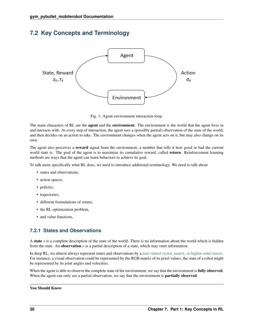
Fig. 1: Agent-environment interaction loop.

The main characters of RL are the agent and the environment. The environment is the world that the agent lives inand interacts with. At every step of interaction, the agent sees a (possibly partial) observation of the state of the world,and then decides on an action to take. The environment changes when the agent acts on it, but may also change on itsown.

The agent also perceives a reward signal from the environment, a number that tells it how good or bad the currentworld state is. The goal of the agent is to maximize its cumulative reward, called return. Reinforcement learningmethods are ways that the agent can learn behaviors to achieve its goal.

To talk more specifically what RL does, we need to introduce additional terminology. We need to talk about

• states and observations,

• action spaces,

• policies,

• trajectories,

• different formulations of return,

• the RL optimization problem,

• and value functions.

7.2.1 States and Observations

A state 𝑠 is a complete description of the state of the world. There is no information about the world which is hiddenfrom the state. An observation 𝑜 is a partial description of a state, which may omit information.

In deep RL, we almost always represent states and observations by a real-valued vector, matrix, or higher-order tensor.For instance, a visual observation could be represented by the RGB matrix of its pixel values; the state of a robot mightbe represented by its joint angles and velocities.

When the agent is able to observe the complete state of the environment, we say that the environment is fully observed.When the agent can only see a partial observation, we say that the environment is partially observed.

You Should Know

30 Chapter 7. Part 1: Key Concepts in RL

gym_pybullet_mobilerobot Documentation

Reinforcement learning notation sometimes puts the symbol for state, 𝑠, in places where it would be technicallymore appropriate to write the symbol for observation, 𝑜. Specifically, this happens when talking about how the agentdecides an action: we often signal in notation that the action is conditioned on the state, when in practice, the action isconditioned on the observation because the agent does not have access to the state.

In our guide, we’ll follow standard conventions for notation, but it should be clear from context which is meant. Ifsomething is unclear, though, please raise an issue! Our goal is to teach, not to confuse.

7.2.2 Action Spaces

Different environments allow different kinds of actions. The set of all valid actions in a given environment is oftencalled the action space. Some environments, like Atari and Go, have discrete action spaces, where only a finitenumber of moves are available to the agent. Other environments, like where the agent controls a robot in a physicalworld, have continuous action spaces. In continuous spaces, actions are real-valued vectors.

This distinction has some quite-profound consequences for methods in deep RL. Some families of algorithms can onlybe directly applied in one case, and would have to be substantially reworked for the other.

7.2.3 Policies

A policy is a rule used by an agent to decide what actions to take. It can be deterministic, in which case it is usuallydenoted by 𝜇:

𝑎𝑡 = 𝜇(𝑠𝑡),

or it may be stochastic, in which case it is usually denoted by 𝜋:

𝑎𝑡 ∼ 𝜋(·|𝑠𝑡).

Because the policy is essentially the agent’s brain, it’s not uncommon to substitute the word “policy” for “agent”, egsaying “The policy is trying to maximize reward.”

In deep RL, we deal with parameterized policies: policies whose outputs are computable functions that depend on aset of parameters (eg the weights and biases of a neural network) which we can adjust to change the behavior via someoptimization algorithm.

We often denote the parameters of such a policy by 𝜃 or 𝜑, and then write this as a subscript on the policy symbol tohighlight the connection:

𝑎𝑡 = 𝜇𝜃(𝑠𝑡)

𝑎𝑡 ∼ 𝜋𝜃(·|𝑠𝑡).

Deterministic Policies

Example: Deterministic Policies. Here is a code snippet for building a simple deterministic policy for a continuousaction space in Tensorflow:

obs = tf.placeholder(shape=(None, obs_dim), dtype=tf.float32)net = mlp(obs, hidden_dims=(64,64), activation=tf.tanh)actions = tf.layers.dense(net, units=act_dim, activation=None)

where mlp is a function that stacks multiple dense layers on top of each other with the given sizes and activation.

7.2. Key Concepts and Terminology 31

gym_pybullet_mobilerobot Documentation

Stochastic Policies

The two most common kinds of stochastic policies in deep RL are categorical policies and diagonal Gaussianpolicies.

Categorical policies can be used in discrete action spaces, while diagonal Gaussian policies are used in continuousaction spaces.

Two key computations are centrally important for using and training stochastic policies:

• sampling actions from the policy,

• and computing log likelihoods of particular actions, log 𝜋𝜃(𝑎|𝑠).

In what follows, we’ll describe how to do these for both categorical and diagonal Gaussian policies.

Categorical Policies

A categorical policy is like a classifier over discrete actions. You build the neural network for a categorical policythe same way you would for a classifier: the input is the observation, followed by some number of layers (possiblyconvolutional or densely-connected, depending on the kind of input), and then you have one final linear layer thatgives you logits for each action, followed by a softmax to convert the logits into probabilities.

Sampling. Given the probabilities for each action, frameworks like Tensorflow have built-in tools for sampling. Forexample, see the tf.distributions.Categorical documentation, or tf.multinomial.

Log-Likelihood. Denote the last layer of probabilities as 𝑃𝜃(𝑠). It is a vector with however many entries as there areactions, so we can treat the actions as indices for the vector. The log likelihood for an action 𝑎 can then be obtainedby indexing into the vector:

log 𝜋𝜃(𝑎|𝑠) = log [𝑃𝜃(𝑠)]𝑎 .

Diagonal Gaussian Policies

A multivariate Gaussian distribution (or multivariate normal distribution, if you prefer) is described by a mean vector,𝜇, and a covariance matrix, Σ. A diagonal Gaussian distribution is a special case where the covariance matrix only hasentries on the diagonal. As a result, we can represent it by a vector.

A diagonal Gaussian policy always has a neural network that maps from observations to mean actions, 𝜇𝜃(𝑠). Thereare two different ways that the covariance matrix is typically represented.

The first way: There is a single vector of log standard deviations, log 𝜎, which is not a function of state: the log 𝜎 arestandalone parameters. (You Should Know: our implementations of VPG, TRPO, and PPO do it this way.)

The second way: There is a neural network that maps from states to log standard deviations, log 𝜎𝜃(𝑠). It mayoptionally share some layers with the mean network.

Note that in both cases we output log standard deviations instead of standard deviations directly. This is because logstds are free to take on any values in (−∞,∞), while stds must be nonnegative. It’s easier to train parameters if youdon’t have to enforce those kinds of constraints. The standard deviations can be obtained immediately from the logstandard deviations by exponentiating them, so we do not lose anything by representing them this way.

Sampling. Given the mean action 𝜇𝜃(𝑠) and standard deviation 𝜎𝜃(𝑠), and a vector 𝑧 of noise from a sphericalGaussian (𝑧 ∼ 𝒩 (0, 𝐼)), an action sample can be computed with

𝑎 = 𝜇𝜃(𝑠) + 𝜎𝜃(𝑠)⊙ 𝑧,

32 Chapter 7. Part 1: Key Concepts in RL

gym_pybullet_mobilerobot Documentation

where ⊙ denotes the elementwise product of two vectors. Standard frameworks have built-in ways to compute thenoise vectors, such as tf.random_normal. Alternatively, you can just provide the mean and standard deviation directlyto a tf.distributions.Normal object and use that to sample.

Log-Likelihood. The log-likelihood of a 𝑘 -dimensional action 𝑎, for a diagonal Gaussian with mean 𝜇 = 𝜇𝜃(𝑠) andstandard deviation 𝜎 = 𝜎𝜃(𝑠), is given by

log 𝜋𝜃(𝑎|𝑠) = −1

2

(𝑘∑𝑖=1

((𝑎𝑖 − 𝜇𝑖)2

𝜎2𝑖

+ 2 log 𝜎𝑖

)+ 𝑘 log 2𝜋

).

7.2.4 Trajectories

A trajectory 𝜏 is a sequence of states and actions in the world,

𝜏 = (𝑠0, 𝑎0, 𝑠1, 𝑎1, ...).

The very first state of the world, 𝑠0, is randomly sampled from the start-state distribution, sometimes denoted by 𝜌0:

𝑠0 ∼ 𝜌0(·).

State transitions (what happens to the world between the state at time 𝑡, 𝑠𝑡, and the state at 𝑡+1, 𝑠𝑡+1), are governed bythe natural laws of the environment, and depend on only the most recent action, 𝑎𝑡. They can be either deterministic,

𝑠𝑡+1 = 𝑓(𝑠𝑡, 𝑎𝑡)

or stochastic,

𝑠𝑡+1 ∼ 𝑃 (·|𝑠𝑡, 𝑎𝑡).

Actions come from an agent according to its policy.

You Should Know

Trajectories are also frequently called episodes or rollouts.

7.2.5 Reward and Return

The reward function 𝑅 is critically important in reinforcement learning. It depends on the current state of the world,the action just taken, and the next state of the world:

𝑟𝑡 = 𝑅(𝑠𝑡, 𝑎𝑡, 𝑠𝑡+1)

although frequently this is simplified to just a dependence on the current state, 𝑟𝑡 = 𝑅(𝑠𝑡), or state-action pair𝑟𝑡 = 𝑅(𝑠𝑡, 𝑎𝑡).

The goal of the agent is to maximize some notion of cumulative reward over a trajectory, but this actually can mean afew things. We’ll notate all of these cases with 𝑅(𝜏), and it will either be clear from context which case we mean, orit won’t matter (because the same equations will apply to all cases).

One kind of return is the finite-horizon undiscounted return, which is just the sum of rewards obtained in a fixedwindow of steps:

𝑅(𝜏) =

𝑇∑𝑡=0

𝑟𝑡.

7.2. Key Concepts and Terminology 33

gym_pybullet_mobilerobot Documentation

Another kind of return is the infinite-horizon discounted return, which is the sum of all rewards ever obtained bythe agent, but discounted by how far off in the future they’re obtained. This formulation of reward includes a discountfactor 𝛾 ∈ (0, 1):

𝑅(𝜏) =

∞∑𝑡=0

𝛾𝑡𝑟𝑡.

Why would we ever want a discount factor, though? Don’t we just want to get all rewards? We do, but the discountfactor is both intuitively appealing and mathematically convenient. On an intuitive level: cash now is better than cashlater. Mathematically: an infinite-horizon sum of rewards may not converge to a finite value, and is hard to deal within equations. But with a discount factor and under reasonable conditions, the infinite sum converges.

You Should Know

While the line between these two formulations of return are quite stark in RL formalism, deep RL practice tends toblur the line a fair bit—for instance, we frequently set up algorithms to optimize the undiscounted return, but usediscount factors in estimating value functions.

7.2.6 The RL Problem

Whatever the choice of return measure (whether infinite-horizon discounted, or finite-horizon undiscounted), andwhatever the choice of policy, the goal in RL is to select a policy which maximizes expected return when the agentacts according to it.

To talk about expected return, we first have to talk about probability distributions over trajectories.

Let’s suppose that both the environment transitions and the policy are stochastic. In this case, the probability of a 𝑇-step trajectory is:

𝑃 (𝜏 |𝜋) = 𝜌0(𝑠0)

𝑇−1∏𝑡=0

𝑃 (𝑠𝑡+1|𝑠𝑡, 𝑎𝑡)𝜋(𝑎𝑡|𝑠𝑡).

The expected return (for whichever measure), denoted by 𝐽(𝜋), is then:

𝐽(𝜋) =

∫𝜏

𝑃 (𝜏 |𝜋)𝑅(𝜏) = 𝜏 ∼ 𝜋𝑅(𝜏).

The central optimization problem in RL can then be expressed by

𝜋* = arg max𝜋

𝐽(𝜋),

with 𝜋* being the optimal policy.

7.2.7 Value Functions

It’s often useful to know the value of a state, or state-action pair. By value, we mean the expected return if you start inthat state or state-action pair, and then act according to a particular policy forever after. Value functions are used, oneway or another, in almost every RL algorithm.

There are four main functions of note here.

1. The On-Policy Value Function, 𝑉 𝜋(𝑠), which gives the expected return if you start in state 𝑠 and always actaccording to policy 𝜋:

34 Chapter 7. Part 1: Key Concepts in RL

gym_pybullet_mobilerobot Documentation

𝑉 𝜋(𝑠) = 𝜏 ∼ 𝜋𝑅(𝜏) |𝑠0 = 𝑠

2. The On-Policy Action-Value Function, 𝑄𝜋(𝑠, 𝑎), which gives the expected return if you start in state 𝑠, takean arbitrary action 𝑎 (which may not have come from the policy), and then forever after act according to policy𝜋:

𝑄𝜋(𝑠, 𝑎) = 𝜏 ∼ 𝜋𝑅(𝜏) |𝑠0 = 𝑠, 𝑎0 = 𝑎

3. The Optimal Value Function, 𝑉 *(𝑠), which gives the expected return if you start in state 𝑠 and always actaccording to the optimal policy in the environment:

𝑉 *(𝑠) = max𝜋

𝜏 ∼ 𝜋𝑅(𝜏) |𝑠0 = 𝑠

4. The Optimal Action-Value Function, 𝑄*(𝑠, 𝑎), which gives the expected return if you start in state 𝑠, take anarbitrary action 𝑎, and then forever after act according to the optimal policy in the environment:

𝑄*(𝑠, 𝑎) = max𝜋

𝜏 ∼ 𝜋𝑅(𝜏) |𝑠0 = 𝑠, 𝑎0 = 𝑎

You Should Know

When we talk about value functions, if we do not make reference to time-dependence, we only mean expected infinite-horizon discounted return. Value functions for finite-horizon undiscounted return would need to accept time as anargument. Can you think about why? Hint: what happens when time’s up?

You Should Know

There are two key connections between the value function and the action-value function that come up pretty often:

𝑉 𝜋(𝑠) = 𝑎 ∼ 𝜋𝑄𝜋(𝑠, 𝑎),

and

𝑉 *(𝑠) = max𝑎

𝑄*(𝑠, 𝑎).

These relations follow pretty directly from the definitions just given: can you prove them?

7.2.8 The Optimal Q-Function and the Optimal Action

There is an important connection between the optimal action-value function 𝑄*(𝑠, 𝑎) and the action selected by theoptimal policy. By definition, 𝑄*(𝑠, 𝑎) gives the expected return for starting in state 𝑠, taking (arbitrary) action 𝑎, andthen acting according to the optimal policy forever after.

7.2. Key Concepts and Terminology 35

gym_pybullet_mobilerobot Documentation

The optimal policy in 𝑠 will select whichever action maximizes the expected return from starting in 𝑠. As a result, ifwe have 𝑄*, we can directly obtain the optimal action, 𝑎*(𝑠), via

𝑎*(𝑠) = arg max𝑎

𝑄*(𝑠, 𝑎).

Note: there may be multiple actions which maximize 𝑄*(𝑠, 𝑎), in which case, all of them are optimal, and the optimalpolicy may randomly select any of them. But there is always an optimal policy which deterministically selects anaction.

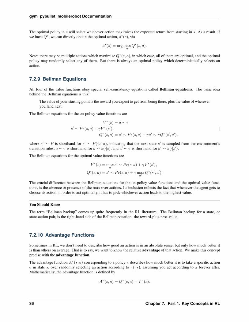
7.2.9 Bellman Equations

All four of the value functions obey special self-consistency equations called Bellman equations. The basic ideabehind the Bellman equations is this:

The value of your starting point is the reward you expect to get from being there, plus the value of whereveryou land next.

The Bellman equations for the on-policy value functions are

𝑉 𝜋(𝑠) = 𝑎 ∼ 𝜋𝑠′ ∼ 𝑃𝑟(𝑠, 𝑎) + 𝛾𝑉 𝜋(𝑠′), [

𝑄𝜋(𝑠, 𝑎) = 𝑠′ ∼ 𝑃𝑟(𝑠, 𝑎) + 𝛾𝑎′ ∼ 𝜋𝑄𝜋(𝑠′, 𝑎′),

where 𝑠′ ∼ 𝑃 is shorthand for 𝑠′ ∼ 𝑃 (·|𝑠, 𝑎), indicating that the next state 𝑠′ is sampled from the environment’stransition rules; 𝑎 ∼ 𝜋 is shorthand for 𝑎 ∼ 𝜋(·|𝑠); and 𝑎′ ∼ 𝜋 is shorthand for 𝑎′ ∼ 𝜋(·|𝑠′).

The Bellman equations for the optimal value functions are

𝑉 *(𝑠) = max𝑎

𝑠′ ∼ 𝑃𝑟(𝑠, 𝑎) + 𝛾𝑉 *(𝑠′),

𝑄*(𝑠, 𝑎) = 𝑠′ ∼ 𝑃𝑟(𝑠, 𝑎) + 𝛾max𝑎′

𝑄*(𝑠′, 𝑎′).

The crucial difference between the Bellman equations for the on-policy value functions and the optimal value func-tions, is the absence or presence of the max over actions. Its inclusion reflects the fact that whenever the agent gets tochoose its action, in order to act optimally, it has to pick whichever action leads to the highest value.

You Should Know

The term “Bellman backup” comes up quite frequently in the RL literature. The Bellman backup for a state, orstate-action pair, is the right-hand side of the Bellman equation: the reward-plus-next-value.

7.2.10 Advantage Functions

Sometimes in RL, we don’t need to describe how good an action is in an absolute sense, but only how much better itis than others on average. That is to say, we want to know the relative advantage of that action. We make this conceptprecise with the advantage function.

The advantage function 𝐴𝜋(𝑠, 𝑎) corresponding to a policy 𝜋 describes how much better it is to take a specific action𝑎 in state 𝑠, over randomly selecting an action according to 𝜋(·|𝑠), assuming you act according to 𝜋 forever after.Mathematically, the advantage function is defined by

𝐴𝜋(𝑠, 𝑎) = 𝑄𝜋(𝑠, 𝑎)− 𝑉 𝜋(𝑠).

36 Chapter 7. Part 1: Key Concepts in RL

gym_pybullet_mobilerobot Documentation

You Should Know

We’ll discuss this more later, but the advantage function is crucially important to policy gradient methods.

7.3 (Optional) Formalism

So far, we’ve discussed the agent’s environment in an informal way, but if you try to go digging through the literature,you’re likely to run into the standard mathematical formalism for this setting: Markov Decision Processes (MDPs).An MDP is a 5-tuple, ⟨𝑆,𝐴,𝑅, 𝑃, 𝜌0⟩, where

• 𝑆 is the set of all valid states,

• 𝐴 is the set of all valid actions,

• 𝑅 : 𝑆 ×𝐴× 𝑆 → R is the reward function, with 𝑟𝑡 = 𝑅(𝑠𝑡, 𝑎𝑡, 𝑠𝑡+1),

• 𝑃 : 𝑆 × 𝐴 → 𝒫(𝑆) is the transition probability function, with 𝑃 (𝑠′|𝑠, 𝑎) being the probability of transitioninginto state 𝑠′ if you start in state 𝑠 and take action 𝑎,

• and 𝜌0 is the starting state distribution.

The name Markov Decision Process refers to the fact that the system obeys the Markov property: transitions onlydepend on the most recent state and action, and no prior history.

7.3. (Optional) Formalism 37

gym_pybullet_mobilerobot Documentation

38 Chapter 7. Part 1: Key Concepts in RL

CHAPTER 8

Part 2: Kinds of RL Algorithms

Table of Contents

• Part 2: Kinds of RL Algorithms

– A Taxonomy of RL Algorithms

– Links to Algorithms in Taxonomy

Now that we’ve gone through the basics of RL terminology and notation, we can cover a little bit of the richer material:the landscape of algorithms in modern RL, and a description of the kinds of trade-offs that go into algorithm design.

8.1 A Taxonomy of RL Algorithms

Fig. 1: A non-exhaustive, but useful taxonomy of algorithms in modern RL. Citations below.

We’ll start this section with a disclaimer: it’s really quite hard to draw an accurate, all-encompassing taxonomy ofalgorithms in the modern RL space, because the modularity of algorithms is not well-represented by a tree structure.Also, to make something that fits on a page and is reasonably digestible in an introduction essay, we have to omit quitea bit of more advanced material (exploration, transfer learning, meta learning, etc). That said, our goals here are

• to highlight the most foundational design choices in deep RL algorithms about what to learn and how to learn it,

• to expose the trade-offs in those choices,

• and to place a few prominent modern algorithms into context with respect to those choices.

8.1.1 Model-Free vs Model-Based RL

One of the most important branching points in an RL algorithm is the question of whether the agent has access to(or learns) a model of the environment. By a model of the environment, we mean a function which predicts state

39

gym_pybullet_mobilerobot Documentation

transitions and rewards.

The main upside to having a model is that it allows the agent to plan by thinking ahead, seeing what would happenfor a range of possible choices, and explicitly deciding between its options. Agents can then distill the results fromplanning ahead into a learned policy. A particularly famous example of this approach is AlphaZero. When this works,it can result in a substantial improvement in sample efficiency over methods that don’t have a model.

The main downside is that a ground-truth model of the environment is usually not available to the agent. Ifan agent wants to use a model in this case, it has to learn the model purely from experience, which creates severalchallenges. The biggest challenge is that bias in the model can be exploited by the agent, resulting in an agent whichperforms well with respect to the learned model, but behaves sub-optimally (or super terribly) in the real environment.Model-learning is fundamentally hard, so even intense effort—being willing to throw lots of time and compute atit—can fail to pay off.

Algorithms which use a model are called model-based methods, and those that don’t are called model-free. Whilemodel-free methods forego the potential gains in sample efficiency from using a model, they tend to be easier toimplement and tune. As of the time of writing this introduction (September 2018), model-free methods are morepopular and have been more extensively developed and tested than model-based methods.

8.1.2 What to Learn

Another critical branching point in an RL algorithm is the question of what to learn. The list of usual suspectsincludes

• policies, either stochastic or deterministic,

• action-value functions (Q-functions),

• value functions,

• and/or environment models.

What to Learn in Model-Free RL

There are two main approaches to representing and training agents with model-free RL:

Policy Optimization. Methods in this family represent a policy explicitly as 𝜋𝜃(𝑎|𝑠). They optimize the parameters 𝜃either directly by gradient ascent on the performance objective 𝐽(𝜋𝜃), or indirectly, by maximizing local approxima-tions of 𝐽(𝜋𝜃). This optimization is almost always performed on-policy, which means that each update only uses datacollected while acting according to the most recent version of the policy. Policy optimization also usually involveslearning an approximator 𝑉𝜑(𝑠) for the on-policy value function 𝑉 𝜋(𝑠), which gets used in figuring out how to updatethe policy.

A couple of examples of policy optimization methods are:

• A2C / A3C, which performs gradient ascent to directly maximize performance,

• and PPO, whose updates indirectly maximize performance, by instead maximizing a surrogate objective func-tion which gives a conservative estimate for how much 𝐽(𝜋𝜃) will change as a result of the update.

Q-Learning. Methods in this family learn an approximator 𝑄𝜃(𝑠, 𝑎) for the optimal action-value function, 𝑄*(𝑠, 𝑎).Typically they use an objective function based on the Bellman equation. This optimization is almost always performedoff-policy, which means that each update can use data collected at any point during training, regardless of how theagent was choosing to explore the environment when the data was obtained. The corresponding policy is obtained viathe connection between 𝑄* and 𝜋*: the actions taken by the Q-learning agent are given by

𝑎(𝑠) = arg max𝑎

𝑄𝜃(𝑠, 𝑎).

Examples of Q-learning methods include

40 Chapter 8. Part 2: Kinds of RL Algorithms

gym_pybullet_mobilerobot Documentation

• DQN, a classic which substantially launched the field of deep RL,

• and C51, a variant that learns a distribution over return whose expectation is 𝑄*.

Trade-offs Between Policy Optimization and Q-Learning. The primary strength of policy optimization methods isthat they are principled, in the sense that you directly optimize for the thing you want. This tends to make them stableand reliable. By contrast, Q-learning methods only indirectly optimize for agent performance, by training𝑄𝜃 to satisfya self-consistency equation. There are many failure modes for this kind of learning, so it tends to be less stable.1 But,Q-learning methods gain the advantage of being substantially more sample efficient when they do work, because theycan reuse data more effectively than policy optimization techniques.

Interpolating Between Policy Optimization and Q-Learning. Serendipitously, policy optimization and Q-learningare not incompatible (and under some circumstances, it turns out, equivalent), and there exist a range of algorithmsthat live in between the two extremes. Algorithms that live on this spectrum are able to carefully trade-off between thestrengths and weaknesses of either side. Examples include

• DDPG, an algorithm which concurrently learns a deterministic policy and a Q-function by using each to improvethe other,

• and SAC, a variant which uses stochastic policies, entropy regularization, and a few other tricks to stabilizelearning and score higher than DDPG on standard benchmarks.

8.1.3 What to Learn in Model-Based RL

Unlike model-free RL, there aren’t a small number of easy-to-define clusters of methods for model-based RL: thereare many orthogonal ways of using models. We’ll give a few examples, but the list is far from exhaustive. In eachcase, the model may either be given or learned.

Background: Pure Planning. The most basic approach never explicitly represents the policy, and instead, uses pureplanning techniques like model-predictive control (MPC) to select actions. In MPC, each time the agent observes theenvironment, it computes a plan which is optimal with respect to the model, where the plan describes all actions totake over some fixed window of time after the present. (Future rewards beyond the horizon may be considered by theplanning algorithm through the use of a learned value function.) The agent then executes the first action of the plan,and immediately discards the rest of it. It computes a new plan each time it prepares to interact with the environment,to avoid using an action from a plan with a shorter-than-desired planning horizon.

• The MBMF work explores MPC with learned environment models on some standard benchmark tasks for deepRL.

Expert Iteration. A straightforward follow-on to pure planning involves using and learning an explicit representationof the policy, 𝜋𝜃(𝑎|𝑠). The agent uses a planning algorithm (like Monte Carlo Tree Search) in the model, generatingcandidate actions for the plan by sampling from its current policy. The planning algorithm produces an action whichis better than what the policy alone would have produced, hence it is an “expert” relative to the policy. The policy isafterwards updated to produce an action more like the planning algorithm’s output.

• The ExIt algorithm uses this approach to train deep neural networks to play Hex.

• AlphaZero is another example of this approach.

Data Augmentation for Model-Free Methods. Use a model-free RL algorithm to train a policy or Q-function, buteither 1) augment real experiences with fictitious ones in updating the agent, or 2) use only fictitous experience forupdating the agent.

• See MBVE for an example of augmenting real experiences with fictitious ones.

• See World Models for an example of using purely fictitious experience to train the agent, which they call “train-ing in the dream.”

1 For more information about how and why Q-learning methods can fail, see 1) this classic paper by Tsitsiklis and van Roy, 2) the (much morerecent) review by Szepesvari (in section 4.3.2), and 3) chapter 11 of Sutton and Barto, especially section 11.3 (on “the deadly triad” of functionapproximation, bootstrapping, and off-policy data, together causing instability in value-learning algorithms).

8.1. A Taxonomy of RL Algorithms 41

gym_pybullet_mobilerobot Documentation

Embedding Planning Loops into Policies. Another approach embeds the planning procedure directly into a policy asa subroutine—so that complete plans become side information for the policy—while training the output of the policywith any standard model-free algorithm. The key concept is that in this framework, the policy can learn to choose howand when to use the plans. This makes model bias less of a problem, because if the model is bad for planning in somestates, the policy can simply learn to ignore it.

• See I2A for an example of agents being endowed with this style of imagination.

8.2 Links to Algorithms in Taxonomy

42 Chapter 8. Part 2: Kinds of RL Algorithms

CHAPTER 9

Part 3: Intro to Policy Optimization

Table of Contents

• Part 3: Intro to Policy Optimization

– Deriving the Simplest Policy Gradient

– Implementing the Simplest Policy Gradient

– Expected Grad-Log-Prob Lemma

– Don’t Let the Past Distract You

– Implementing Reward-to-Go Policy Gradient

– Baselines in Policy Gradients

– Other Forms of the Policy Gradient

– Recap

In this section, we’ll discuss the mathematical foundations of policy optimization algorithms, and connect the materialto sample code. We will cover three key results in the theory of policy gradients:

• the simplest equation describing the gradient of policy performance with respect to policy parameters,

• a rule which allows us to drop useless terms from that expression,

• and a rule which allows us to add useful terms to that expression.

In the end, we’ll tie those results together and describe the advantage-based expression for the policy gradient—theversion we use in our Vanilla Policy Gradient implementation.

43

gym_pybullet_mobilerobot Documentation

9.1 Deriving the Simplest Policy Gradient

Here, we consider the case of a stochastic, parameterized policy, 𝜋𝜃. We aim to maximize the expected return 𝐽(𝜋𝜃) =𝜏 ∼ 𝜋𝜃𝑅(𝜏). For the purposes of this derivation, we’ll take 𝑅(𝜏) to give the finite-horizon undiscounted return, butthe derivation for the infinite-horizon discounted return setting is almost identical.

We would like to optimize the policy by gradient ascent, eg

𝜃𝑘+1 = 𝜃𝑘 + 𝛼 ∇𝜃𝐽(𝜋𝜃)|𝜃𝑘 .

The gradient of policy performance, ∇𝜃𝐽(𝜋𝜃), is called the policy gradient, and algorithms that optimize the policythis way are called policy gradient algorithms. (Examples include Vanilla Policy Gradient and TRPO. PPO is oftenreferred to as a policy gradient algorithm, though this is slightly inaccurate.)

To actually use this algorithm, we need an expression for the policy gradient which we can numerically compute. Thisinvolves two steps: 1) deriving the analytical gradient of policy performance, which turns out to have the form of anexpected value, and then 2) forming a sample estimate of that expected value, which can be computed with data froma finite number of agent-environment interaction steps.

In this subsection, we’ll find the simplest form of that expression. In later subsections, we’ll show how to improve onthe simplest form to get the version we actually use in standard policy gradient implementations.

We’ll begin by laying out a few facts which are useful for deriving the analytical gradient.

1. Probability of a Trajectory. The probability of a trajectory 𝜏 = (𝑠0, 𝑎0, ..., 𝑠𝑇+1) given that actions come from𝜋𝜃 is

𝑃 (𝜏 |𝜃) = 𝜌0(𝑠0)

𝑇∏𝑡=0

𝑃 (𝑠𝑡+1|𝑠𝑡, 𝑎𝑡)𝜋𝜃(𝑎𝑡|𝑠𝑡).

2. The Log-Derivative Trick. The log-derivative trick is based on a simple rule from calculus: the derivative of log 𝑥with respect to 𝑥 is 1/𝑥. When rearranged and combined with chain rule, we get:

∇𝜃𝑃 (𝜏 |𝜃) = 𝑃 (𝜏 |𝜃)∇𝜃 log𝑃 (𝜏 |𝜃).

3. Log-Probability of a Trajectory. The log-prob of a trajectory is just

log𝑃 (𝜏 |𝜃) = log 𝜌0(𝑠0) +

𝑇∑𝑡=0

(log𝑃 (𝑠𝑡+1|𝑠𝑡, 𝑎𝑡) + log 𝜋𝜃(𝑎𝑡|𝑠𝑡)

).

4. Gradients of Environment Functions. The environment has no dependence on 𝜃, so gradients of 𝜌0(𝑠0),𝑃 (𝑠𝑡+1|𝑠𝑡, 𝑎𝑡), and 𝑅(𝜏) are zero.

5. Grad-Log-Prob of a Trajectory. The gradient of the log-prob of a trajectory is thus

∇𝜃 log𝑃 (𝜏 |𝜃) = ∇𝜃 log 𝜌0(𝑠0) +

𝑇∑𝑡=0

(∇𝜃 log𝑃 (𝑠𝑡+1|𝑠𝑡, 𝑎𝑡) +∇𝜃 log 𝜋𝜃(𝑎𝑡|𝑠𝑡)

)

=

𝑇∑𝑡=0

∇𝜃 log 𝜋𝜃(𝑎𝑡|𝑠𝑡).

Putting it all together, we derive the following:

44 Chapter 9. Part 3: Intro to Policy Optimization

gym_pybullet_mobilerobot Documentation

Derivation for Basic Policy Gradient

∇𝜃𝐽(𝜋𝜃) = ∇𝜃𝜏 ∼ 𝜋𝜃𝑅(𝜏)

= ∇𝜃∫𝜏

𝑃 (𝜏 |𝜃)𝑅(𝜏) Expand expectation

=

∫𝜏

∇𝜃𝑃 (𝜏 |𝜃)𝑅(𝜏) Bring gradient under integral

=

∫𝜏

𝑃 (𝜏 |𝜃)∇𝜃 log𝑃 (𝜏 |𝜃)𝑅(𝜏) Log-derivative trick

= 𝜏 ∼ 𝜋𝜃∇𝜃 log𝑃 (𝜏 |𝜃)𝑅(𝜏) Return to expectation form

∴ ∇𝜃𝐽(𝜋𝜃) = 𝜏 ∼ 𝜋𝜃𝑇∑𝑡=0

∇𝜃 log 𝜋𝜃(𝑎𝑡|𝑠𝑡)𝑅(𝜏) Expression for grad-log-prob

This is an expectation, which means that we can estimate it with a sample mean. If we collect a set of trajectories𝒟 = {𝜏𝑖}𝑖=1,...,𝑁 where each trajectory is obtained by letting the agent act in the environment using the policy 𝜋𝜃, thepolicy gradient can be estimated with

𝑔 =1

|𝒟|∑𝜏∈𝒟

𝑇∑𝑡=0

∇𝜃 log 𝜋𝜃(𝑎𝑡|𝑠𝑡)𝑅(𝜏),

where |𝒟| is the number of trajectories in 𝒟 (here, 𝑁 ).

This last expression is the simplest version of the computable expression we desired. Assuming that we have repre-sented our policy in a way which allows us to calculate ∇𝜃 log 𝜋𝜃(𝑎|𝑠), and if we are able to run the policy in theenvironment to collect the trajectory dataset, we can compute the policy gradient and take an update step.

9.2 Implementing the Simplest Policy Gradient

We give a short Tensorflow implementation of this simple version of the policy gradient algorithm in spinup/examples/pg_math/1_simple_pg.py. (It can also be viewed on github.) It is only 122 lines long, so wehighly recommend reading through it in depth. While we won’t go through the entirety of the code here, we’llhighlight and explain a few important pieces.

1. Making the Policy Network.

25 # make core of policy network26 obs_ph = tf.placeholder(shape=(None, obs_dim), dtype=tf.float32)27 logits = mlp(obs_ph, sizes=hidden_sizes+[n_acts])28

29 # make action selection op (outputs int actions, sampled from policy)30 actions = tf.squeeze(tf.multinomial(logits=logits,num_samples=1), axis=1)

This block builds a feedforward neural network categorical policy. (See the Stochastic Policies section in Part 1 fora refresher.) The logits tensor can be used to construct log-probabilities and probabilities for actions, and theactions tensor samples actions based on the probabilities implied by logits.

2. Making the Loss Function.

32 # make loss function whose gradient, for the right data, is policy gradient33 weights_ph = tf.placeholder(shape=(None,), dtype=tf.float32)

(continues on next page)

9.2. Implementing the Simplest Policy Gradient 45

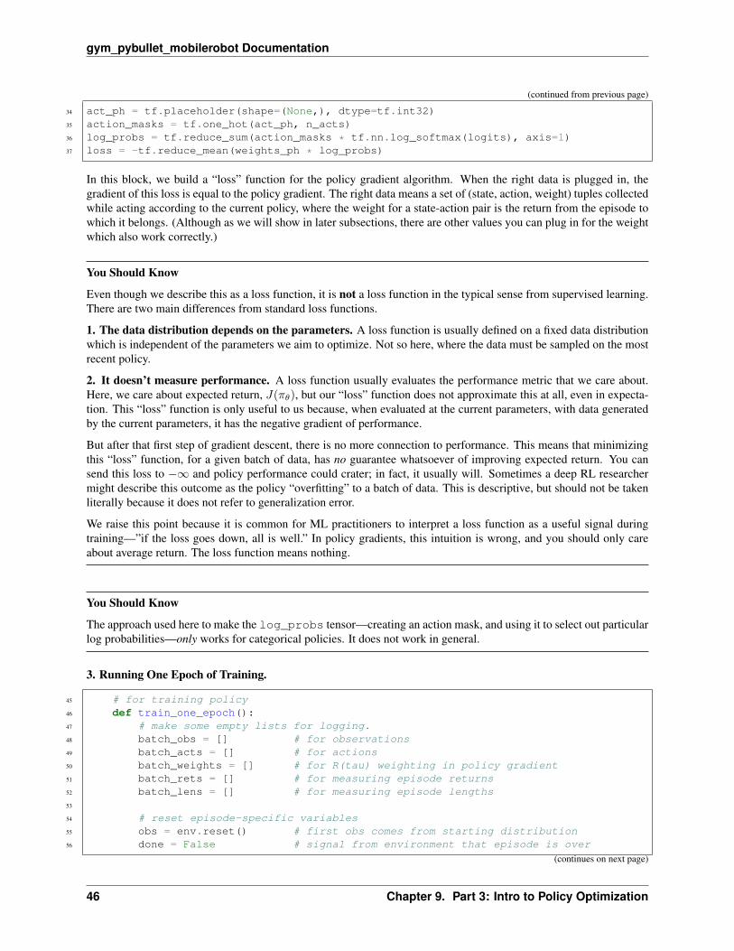
gym_pybullet_mobilerobot Documentation

(continued from previous page)

34 act_ph = tf.placeholder(shape=(None,), dtype=tf.int32)35 action_masks = tf.one_hot(act_ph, n_acts)36 log_probs = tf.reduce_sum(action_masks * tf.nn.log_softmax(logits), axis=1)37 loss = -tf.reduce_mean(weights_ph * log_probs)

In this block, we build a “loss” function for the policy gradient algorithm. When the right data is plugged in, thegradient of this loss is equal to the policy gradient. The right data means a set of (state, action, weight) tuples collectedwhile acting according to the current policy, where the weight for a state-action pair is the return from the episode towhich it belongs. (Although as we will show in later subsections, there are other values you can plug in for the weightwhich also work correctly.)

You Should Know

Even though we describe this as a loss function, it is not a loss function in the typical sense from supervised learning.There are two main differences from standard loss functions.

1. The data distribution depends on the parameters. A loss function is usually defined on a fixed data distributionwhich is independent of the parameters we aim to optimize. Not so here, where the data must be sampled on the mostrecent policy.

2. It doesn’t measure performance. A loss function usually evaluates the performance metric that we care about.Here, we care about expected return, 𝐽(𝜋𝜃), but our “loss” function does not approximate this at all, even in expecta-tion. This “loss” function is only useful to us because, when evaluated at the current parameters, with data generatedby the current parameters, it has the negative gradient of performance.

But after that first step of gradient descent, there is no more connection to performance. This means that minimizingthis “loss” function, for a given batch of data, has no guarantee whatsoever of improving expected return. You cansend this loss to −∞ and policy performance could crater; in fact, it usually will. Sometimes a deep RL researchermight describe this outcome as the policy “overfitting” to a batch of data. This is descriptive, but should not be takenliterally because it does not refer to generalization error.

We raise this point because it is common for ML practitioners to interpret a loss function as a useful signal duringtraining—”if the loss goes down, all is well.” In policy gradients, this intuition is wrong, and you should only careabout average return. The loss function means nothing.

You Should Know

The approach used here to make the log_probs tensor—creating an action mask, and using it to select out particularlog probabilities—only works for categorical policies. It does not work in general.

3. Running One Epoch of Training.

45 # for training policy46 def train_one_epoch():47 # make some empty lists for logging.48 batch_obs = [] # for observations49 batch_acts = [] # for actions50 batch_weights = [] # for R(tau) weighting in policy gradient51 batch_rets = [] # for measuring episode returns52 batch_lens = [] # for measuring episode lengths53

54 # reset episode-specific variables55 obs = env.reset() # first obs comes from starting distribution56 done = False # signal from environment that episode is over

(continues on next page)

46 Chapter 9. Part 3: Intro to Policy Optimization

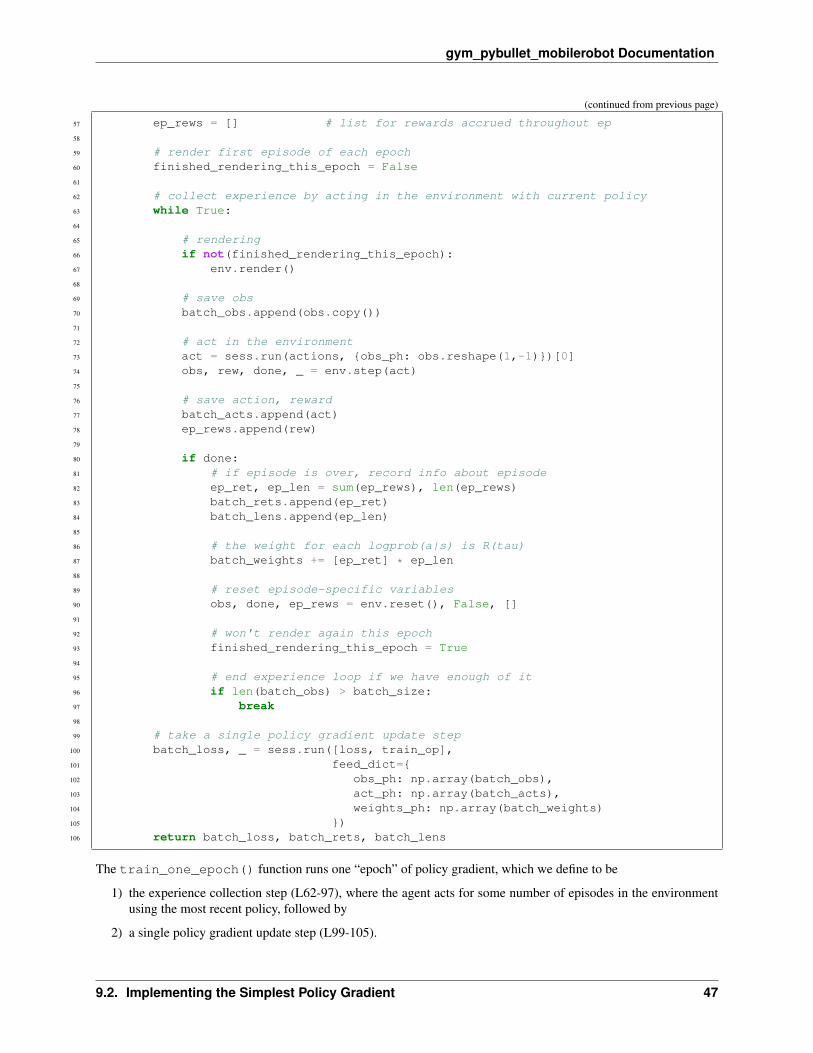
gym_pybullet_mobilerobot Documentation

(continued from previous page)

57 ep_rews = [] # list for rewards accrued throughout ep58

59 # render first episode of each epoch60 finished_rendering_this_epoch = False61

62 # collect experience by acting in the environment with current policy63 while True:64

65 # rendering66 if not(finished_rendering_this_epoch):67 env.render()68

69 # save obs70 batch_obs.append(obs.copy())71

72 # act in the environment73 act = sess.run(actions, {obs_ph: obs.reshape(1,-1)})[0]74 obs, rew, done, _ = env.step(act)75

76 # save action, reward77 batch_acts.append(act)78 ep_rews.append(rew)79

80 if done:81 # if episode is over, record info about episode82 ep_ret, ep_len = sum(ep_rews), len(ep_rews)83 batch_rets.append(ep_ret)84 batch_lens.append(ep_len)85

86 # the weight for each logprob(a|s) is R(tau)87 batch_weights += [ep_ret] * ep_len88

89 # reset episode-specific variables90 obs, done, ep_rews = env.reset(), False, []91

92 # won't render again this epoch93 finished_rendering_this_epoch = True94

95 # end experience loop if we have enough of it96 if len(batch_obs) > batch_size:97 break98

99 # take a single policy gradient update step100 batch_loss, _ = sess.run([loss, train_op],101 feed_dict={102 obs_ph: np.array(batch_obs),103 act_ph: np.array(batch_acts),104 weights_ph: np.array(batch_weights)105 })106 return batch_loss, batch_rets, batch_lens

The train_one_epoch() function runs one “epoch” of policy gradient, which we define to be

1) the experience collection step (L62-97), where the agent acts for some number of episodes in the environmentusing the most recent policy, followed by

2) a single policy gradient update step (L99-105).

9.2. Implementing the Simplest Policy Gradient 47

gym_pybullet_mobilerobot Documentation

The main loop of the algorithm just repeatedly calls train_one_epoch().

9.3 Expected Grad-Log-Prob Lemma

In this subsection, we will derive an intermediate result which is extensively used throughout the theory of policygradients. We will call it the Expected Grad-Log-Prob (EGLP) lemma.1

EGLP Lemma. Suppose that 𝑃𝜃 is a parameterized probability distribution over a random variable, 𝑥. Then:

𝑥 ∼ 𝑃𝜃∇𝜃 log𝑃𝜃(𝑥) = 0.

Proof

Recall that all probability distributions are normalized:∫𝑥

𝑃𝜃(𝑥) = 1.

Take the gradient of both sides of the normalization condition:

∇𝜃∫𝑥

𝑃𝜃(𝑥) = ∇𝜃1 = 0.

Use the log derivative trick to get:

0 = ∇𝜃∫𝑥

𝑃𝜃(𝑥)

=

∫𝑥

∇𝜃𝑃𝜃(𝑥)

=

∫𝑥

𝑃𝜃(𝑥)∇𝜃 log𝑃𝜃(𝑥)

∴ 0 = 𝑥 ∼ 𝑃𝜃∇𝜃 log𝑃𝜃(𝑥).

9.4 Don’t Let the Past Distract You

Examine our most recent expression for the policy gradient:

∇𝜃𝐽(𝜋𝜃) = 𝜏 ∼ 𝜋𝜃𝑇∑𝑡=0

∇𝜃 log 𝜋𝜃(𝑎𝑡|𝑠𝑡)𝑅(𝜏).

Taking a step with this gradient pushes up the log-probabilities of each action in proportion to 𝑅(𝜏), the sum of allrewards ever obtained. But this doesn’t make much sense.

Agents should really only reinforce actions on the basis of their consequences. Rewards obtained before taking anaction have no bearing on how good that action was: only rewards that come after.

It turns out that this intuition shows up in the math, and we can show that the policy gradient can also be expressed by

∇𝜃𝐽(𝜋𝜃) = 𝜏 ∼ 𝜋𝜃𝑇∑𝑡=0

∇𝜃 log 𝜋𝜃(𝑎𝑡|𝑠𝑡)𝑇∑𝑡′=𝑡

𝑅(𝑠𝑡′ , 𝑎𝑡′ , 𝑠𝑡′+1).

1 The author of this article is not aware of this lemma being given a standard name anywhere in the literature. But given how often it comes up,it seems pretty worthwhile to give it some kind of name for ease of reference.

48 Chapter 9. Part 3: Intro to Policy Optimization

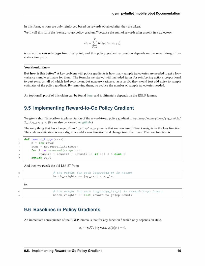
gym_pybullet_mobilerobot Documentation

In this form, actions are only reinforced based on rewards obtained after they are taken.

We’ll call this form the “reward-to-go policy gradient,” because the sum of rewards after a point in a trajectory,

��𝑡.=

𝑇∑𝑡′=𝑡

𝑅(𝑠𝑡′ , 𝑎𝑡′ , 𝑠𝑡′+1),

is called the reward-to-go from that point, and this policy gradient expression depends on the reward-to-go fromstate-action pairs.

You Should Know

But how is this better? A key problem with policy gradients is how many sample trajectories are needed to get a low-variance sample estimate for them. The formula we started with included terms for reinforcing actions proportionalto past rewards, all of which had zero mean, but nonzero variance: as a result, they would just add noise to sampleestimates of the policy gradient. By removing them, we reduce the number of sample trajectories needed.

An (optional) proof of this claim can be found here, and it ultimately depends on the EGLP lemma.

9.5 Implementing Reward-to-Go Policy Gradient

We give a short Tensorflow implementation of the reward-to-go policy gradient in spinup/examples/pg_math/2_rtg_pg.py. (It can also be viewed on github.)

The only thing that has changed from 1_simple_pg.py is that we now use different weights in the loss function.The code modification is very slight: we add a new function, and change two other lines. The new function is:

12 def reward_to_go(rews):13 n = len(rews)14 rtgs = np.zeros_like(rews)15 for i in reversed(range(n)):16 rtgs[i] = rews[i] + (rtgs[i+1] if i+1 < n else 0)17 return rtgs

And then we tweak the old L86-87 from:

86 # the weight for each logprob(a|s) is R(tau)87 batch_weights += [ep_ret] * ep_len

to:

93 # the weight for each logprob(a_t|s_t) is reward-to-go from t94 batch_weights += list(reward_to_go(ep_rews))

9.6 Baselines in Policy Gradients

An immediate consequence of the EGLP lemma is that for any function 𝑏 which only depends on state,

𝑎𝑡 ∼ 𝜋𝜃∇𝜃 log 𝜋𝜃(𝑎𝑡|𝑠𝑡)𝑏(𝑠𝑡) = 0.

9.5. Implementing Reward-to-Go Policy Gradient 49

gym_pybullet_mobilerobot Documentation

This allows us to add or subtract any number of terms like this from our expression for the policy gradient, withoutchanging it in expectation:

∇𝜃𝐽(𝜋𝜃) = 𝜏 ∼ 𝜋𝜃𝑇∑𝑡=0

∇𝜃 log 𝜋𝜃(𝑎𝑡|𝑠𝑡)

(𝑇∑𝑡′=𝑡

𝑅(𝑠𝑡′ , 𝑎𝑡′ , 𝑠𝑡′+1)− 𝑏(𝑠𝑡)

).

Any function 𝑏 used in this way is called a baseline.

The most common choice of baseline is the on-policy value function 𝑉 𝜋(𝑠𝑡). Recall that this is the average return anagent gets if it starts in state 𝑠𝑡 and then acts according to policy 𝜋 for the rest of its life.

Empirically, the choice 𝑏(𝑠𝑡) = 𝑉 𝜋(𝑠𝑡) has the desirable effect of reducing variance in the sample estimate for thepolicy gradient. This results in faster and more stable policy learning. It is also appealing from a conceptual angle: itencodes the intuition that if an agent gets what it expected, it should “feel” neutral about it.

You Should Know

In practice, 𝑉 𝜋(𝑠𝑡) cannot be computed exactly, so it has to be approximated. This is usually done with a neuralnetwork, 𝑉𝜑(𝑠𝑡), which is updated concurrently with the policy (so that the value network always approximates thevalue function of the most recent policy).

The simplest method for learning 𝑉𝜑, used in most implementations of policy optimization algorithms (including VPG,TRPO, PPO, and A2C), is to minimize a mean-squared-error objective:

𝜑𝑘 = arg min𝜑𝑠𝑡, ��𝑡 ∼ 𝜋𝑘

(𝑉𝜑(𝑠𝑡)− ��𝑡

)2,

where 𝜋𝑘 is the policy at epoch 𝑘. This is done with one or more steps of gradient descent, starting from the previousvalue parameters 𝜑𝑘−1.

9.7 Other Forms of the Policy Gradient

What we have seen so far is that the policy gradient has the general form

∇𝜃𝐽(𝜋𝜃) = 𝜏 ∼ 𝜋𝜃𝑇∑𝑡=0

∇𝜃 log 𝜋𝜃(𝑎𝑡|𝑠𝑡)Φ𝑡,

where Φ𝑡 could be any of

Φ𝑡 = 𝑅(𝜏),

or

Φ𝑡 =

𝑇∑𝑡′=𝑡

𝑅(𝑠𝑡′ , 𝑎𝑡′ , 𝑠𝑡′+1),

or

Φ𝑡 =

𝑇∑𝑡′=𝑡

𝑅(𝑠𝑡′ , 𝑎𝑡′ , 𝑠𝑡′+1)− 𝑏(𝑠𝑡).

50 Chapter 9. Part 3: Intro to Policy Optimization

gym_pybullet_mobilerobot Documentation

All of these choices lead to the same expected value for the policy gradient, despite having different variances. It turnsout that there are two more valid choices of weights Φ𝑡 which are important to know.

1. On-Policy Action-Value Function. The choice

Φ𝑡 = 𝑄𝜋𝜃 (𝑠𝑡, 𝑎𝑡)

is also valid. See this page for an (optional) proof of this claim.

2. The Advantage Function. Recall that the advantage of an action, defined by 𝐴𝜋(𝑠𝑡, 𝑎𝑡) = 𝑄𝜋(𝑠𝑡, 𝑎𝑡) − 𝑉 𝜋(𝑠𝑡),describes how much better or worse it is than other actions on average (relative to the current policy). This choice,

Φ𝑡 = 𝐴𝜋𝜃 (𝑠𝑡, 𝑎𝑡)

is also valid. The proof is that it’s equivalent to using Φ𝑡 = 𝑄𝜋𝜃 (𝑠𝑡, 𝑎𝑡) and then using a value function baseline,which we are always free to do.

You Should Know

The formulation of policy gradients with advantage functions is extremely common, and there are many different waysof estimating the advantage function used by different algorithms.

You Should Know

For a more detailed treatment of this topic, you should read the paper on Generalized Advantage Estimation (GAE),which goes into depth about different choices of Φ𝑡 in the background sections.

That paper then goes on to describe GAE, a method for approximating the advantage function in policy optimizationalgorithms which enjoys widespread use. For instance, Spinning Up’s implementations of VPG, TRPO, and PPOmake use of it. As a result, we strongly advise you to study it.

9.8 Recap

In this chapter, we described the basic theory of policy gradient methods and connected some of the early results tocode examples. The interested student should continue from here by studying how the later results (value functionbaselines and the advantage formulation of policy gradients) translate into Spinning Up’s implementation of VanillaPolicy Gradient.

9.8. Recap 51

gym_pybullet_mobilerobot Documentation

52 Chapter 9. Part 3: Intro to Policy Optimization

CHAPTER 10

Spinning Up as a Deep RL Researcher

By Joshua Achiam, October 13th, 2018

Table of Contents

• Spinning Up as a Deep RL Researcher

– The Right Background

– Learn by Doing

– Developing a Research Project

– Doing Rigorous Research in RL

– Closing Thoughts

– PS: Other Resources

– References

If you’re an aspiring deep RL researcher, you’ve probably heard all kinds of things about deep RL by this point.You know that it’s hard and it doesn’t always work. That even when you’re following a recipe, reproducibility is achallenge. And that if you’re starting from scratch, the learning curve is incredibly steep. It’s also the case that thereare a lot of great resources out there, but the material is new enough that there’s not a clear, well-charted path tomastery. The goal of this column is to help you get past the initial hurdle, and give you a clear sense of how to spinup as a deep RL researcher. In particular, this will outline a useful curriculum for increasing raw knowledge, whileinterleaving it with the odds and ends that lead to better research.

10.1 The Right Background

Build up a solid mathematical background. From probability and statistics, feel comfortable with random variables,Bayes’ theorem, chain rule of probability, expected values, standard deviations, and importance sampling. Frommultivariate calculus, understand gradients and (optionally, but it’ll help) Taylor series expansions.

53

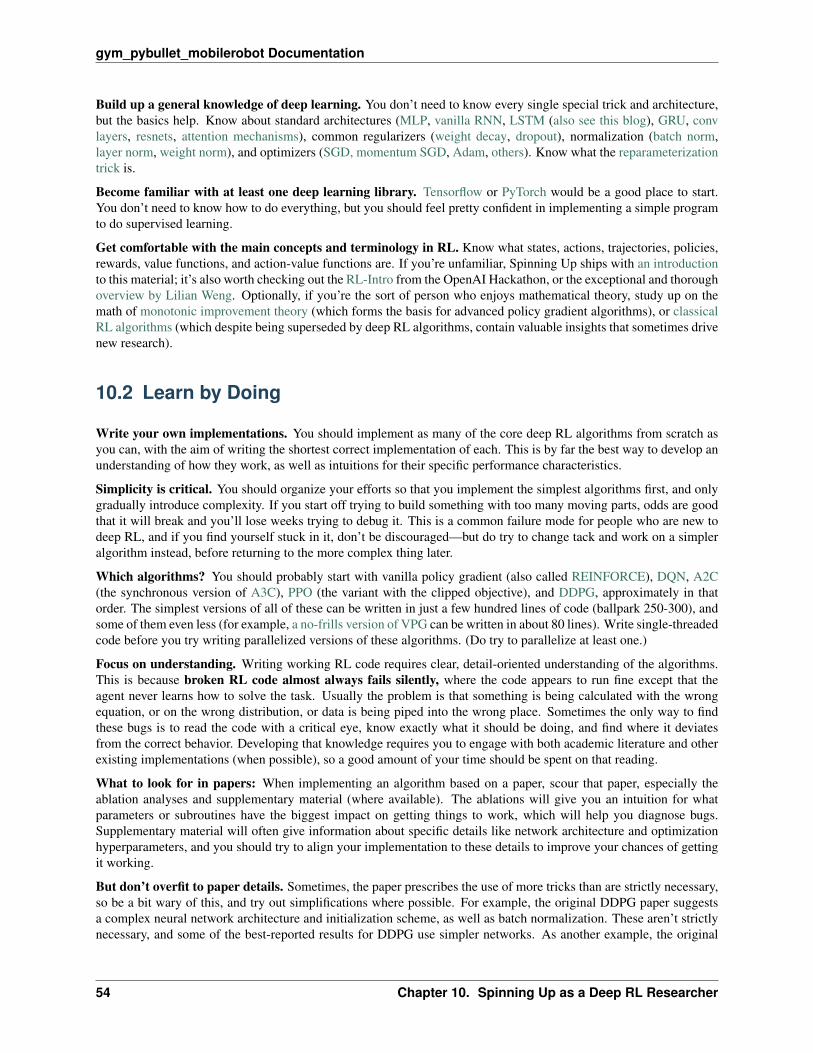
gym_pybullet_mobilerobot Documentation

Build up a general knowledge of deep learning. You don’t need to know every single special trick and architecture,but the basics help. Know about standard architectures (MLP, vanilla RNN, LSTM (also see this blog), GRU, convlayers, resnets, attention mechanisms), common regularizers (weight decay, dropout), normalization (batch norm,layer norm, weight norm), and optimizers (SGD, momentum SGD, Adam, others). Know what the reparameterizationtrick is.

Become familiar with at least one deep learning library. Tensorflow or PyTorch would be a good place to start.You don’t need to know how to do everything, but you should feel pretty confident in implementing a simple programto do supervised learning.

Get comfortable with the main concepts and terminology in RL. Know what states, actions, trajectories, policies,rewards, value functions, and action-value functions are. If you’re unfamiliar, Spinning Up ships with an introductionto this material; it’s also worth checking out the RL-Intro from the OpenAI Hackathon, or the exceptional and thoroughoverview by Lilian Weng. Optionally, if you’re the sort of person who enjoys mathematical theory, study up on themath of monotonic improvement theory (which forms the basis for advanced policy gradient algorithms), or classicalRL algorithms (which despite being superseded by deep RL algorithms, contain valuable insights that sometimes drivenew research).

10.2 Learn by Doing

Write your own implementations. You should implement as many of the core deep RL algorithms from scratch asyou can, with the aim of writing the shortest correct implementation of each. This is by far the best way to develop anunderstanding of how they work, as well as intuitions for their specific performance characteristics.

Simplicity is critical. You should organize your efforts so that you implement the simplest algorithms first, and onlygradually introduce complexity. If you start off trying to build something with too many moving parts, odds are goodthat it will break and you’ll lose weeks trying to debug it. This is a common failure mode for people who are new todeep RL, and if you find yourself stuck in it, don’t be discouraged—but do try to change tack and work on a simpleralgorithm instead, before returning to the more complex thing later.

Which algorithms? You should probably start with vanilla policy gradient (also called REINFORCE), DQN, A2C(the synchronous version of A3C), PPO (the variant with the clipped objective), and DDPG, approximately in thatorder. The simplest versions of all of these can be written in just a few hundred lines of code (ballpark 250-300), andsome of them even less (for example, a no-frills version of VPG can be written in about 80 lines). Write single-threadedcode before you try writing parallelized versions of these algorithms. (Do try to parallelize at least one.)

Focus on understanding. Writing working RL code requires clear, detail-oriented understanding of the algorithms.This is because broken RL code almost always fails silently, where the code appears to run fine except that theagent never learns how to solve the task. Usually the problem is that something is being calculated with the wrongequation, or on the wrong distribution, or data is being piped into the wrong place. Sometimes the only way to findthese bugs is to read the code with a critical eye, know exactly what it should be doing, and find where it deviatesfrom the correct behavior. Developing that knowledge requires you to engage with both academic literature and otherexisting implementations (when possible), so a good amount of your time should be spent on that reading.

What to look for in papers: When implementing an algorithm based on a paper, scour that paper, especially theablation analyses and supplementary material (where available). The ablations will give you an intuition for whatparameters or subroutines have the biggest impact on getting things to work, which will help you diagnose bugs.Supplementary material will often give information about specific details like network architecture and optimizationhyperparameters, and you should try to align your implementation to these details to improve your chances of gettingit working.

But don’t overfit to paper details. Sometimes, the paper prescribes the use of more tricks than are strictly necessary,so be a bit wary of this, and try out simplifications where possible. For example, the original DDPG paper suggestsa complex neural network architecture and initialization scheme, as well as batch normalization. These aren’t strictlynecessary, and some of the best-reported results for DDPG use simpler networks. As another example, the original

54 Chapter 10. Spinning Up as a Deep RL Researcher

gym_pybullet_mobilerobot Documentation

A3C paper uses asynchronous updates from the various actor-learners, but it turns out that synchronous updates workabout as well.

Don’t overfit to existing implementations either. Study existing implementations for inspiration, but be careful notto overfit to the engineering details of those implementations. RL libraries frequently make choices for abstractionthat are good for code reuse between algorithms, but which are unnecessary if you’re only writing a single algorithmor supporting a single use case.

Iterate fast in simple environments. To debug your implementations, try them with simple environments wherelearning should happen quickly, like CartPole-v0, InvertedPendulum-v0, FrozenLake-v0, and HalfCheetah-v2 (witha short time horizon—only 100 or 250 steps instead of the full 1000) from the OpenAI Gym. Don’t try to run analgorithm in Atari or a complex Humanoid environment if you haven’t first verified that it works on the simplestpossible toy task. Your ideal experiment turnaround-time at the debug stage is <5 minutes (on your local machine)or slightly longer but not much. These small-scale experiments don’t require any special hardware, and can be runwithout too much trouble on CPUs.

If it doesn’t work, assume there’s a bug. Spend a lot of effort searching for bugs before you resort to tweakinghyperparameters: usually it’s a bug. Bad hyperparameters can significantly degrade RL performance, but if you’reusing hyperparameters similar to the ones in papers and standard implementations, those will probably not be theissue. Also worth keeping in mind: sometimes things will work in one environment even when you have a breakingbug, so make sure to test in more than one environment once your results look promising.

Measure everything. Do a lot of instrumenting to see what’s going on under-the-hood. The more stats about thelearning process you read out at each iteration, the easier it is to debug—after all, you can’t tell it’s broken if you can’tsee that it’s breaking. I personally like to look at the mean/std/min/max for cumulative rewards, episode lengths, andvalue function estimates, along with the losses for the objectives, and the details of any exploration parameters (likemean entropy for stochastic policy optimization, or current epsilon for epsilon-greedy as in DQN). Also, watch videosof your agent’s performance every now and then; this will give you some insights you wouldn’t get otherwise.

Scale experiments when things work. After you have an implementation of an RL algorithm that seems to work cor-rectly in the simplest environments, test it out on harder environments. Experiments at this stage will take longer—onthe order of somewhere between a few hours and a couple of days, depending. Specialized hardware—like a beefyGPU or a 32-core machine—might be useful at this point, and you should consider looking into cloud computingresources like AWS or GCE.

Keep these habits! These habits are worth keeping beyond the stage where you’re just learning about deep RL—theywill accelerate your research!

10.3 Developing a Research Project

Once you feel reasonably comfortable with the basics in deep RL, you should start pushing on the boundaries anddoing research. To get there, you’ll need an idea for a project.

Start by exploring the literature to become aware of topics in the field. There are a wide range of topics you mightfind interesting: sample efficiency, exploration, transfer learning, hierarchy, memory, model-based RL, meta learning,and multi-agent, to name a few. If you’re looking for inspiration, or just want to get a rough sense of what’s out there,check out Spinning Up’s key papers list. Find a paper that you enjoy on one of these subjects—something that inspiresyou—and read it thoroughly. Use the related work section and citations to find closely-related papers and do a deepdive in the literature. You’ll start to figure out where the unsolved problems are and where you can make an impact.

Approaches to idea-generation: There are a many different ways to start thinking about ideas for projects, and theframe you choose influences how the project might evolve and what risks it will face. Here are a few examples:

Frame 1: Improving on an Existing Approach. This is the incrementalist angle, where you try to get performancegains in an established problem setting by tweaking an existing algorithm. Reimplementing prior work is super helpfulhere, because it exposes you to the ways that existing algorithms are brittle and could be improved. A novice will findthis the most accessible frame, but it can also be worthwhile for researchers at any level of experience. While some

10.3. Developing a Research Project 55

gym_pybullet_mobilerobot Documentation

researchers find incrementalism less exciting, some of the most impressive achievements in machine learning havecome from work of this nature.

Because projects like these are tied to existing methods, they are by nature narrowly scoped and can wrap up quickly(a few months), which may be desirable (especially when starting out as a researcher). But this also sets up the risks:it’s possible that the tweaks you have in mind for an algorithm may fail to improve it, in which case, unless you comeup with more tweaks, the project is just over and you have no clear signal on what to do next.

Frame 2: Focusing on Unsolved Benchmarks. Instead of thinking about how to improve an existing method, youaim to succeed on a task that no one has solved before. For example: achieving perfect generalization from traininglevels to test levels in the Sonic domain or Gym Retro. When you hammer away at an unsolved task, you might try awide variety of methods, including prior approaches and new ones that you invent for the project. It is possible for anovice to approch this kind of problem, but there will be a steeper learning curve.

Projects in this frame have a broad scope and can go on for a while (several months to a year-plus). The main risk isthat the benchmark is unsolvable without a substantial breakthrough, meaning that it would be easy to spend a lot oftime without making any progress on it. But even if a project like this fails, it often leads the researcher to many newinsights that become fertile soil for the next project.

Frame 3: Create a New Problem Setting. Instead of thinking about existing methods or current grand challenges,think of an entirely different conceptual problem that hasn’t been studied yet. Then, figure out how to make progresson it. For projects along these lines, a standard benchmark probably doesn’t exist yet, and you will have to design one.This can be a huge challenge, but it’s worth embracing—great benchmarks move the whole field forward.

Problems in this frame come up when they come up—it’s hard to go looking for them.

Avoid reinventing the wheel. When you come up with a good idea that you want to start testing, that’s great! Butwhile you’re still in the early stages with it, do the most thorough check you can to make sure it hasn’t already beendone. It can be pretty disheartening to get halfway through a project, and only then discover that there’s already apaper about your idea. It’s especially frustrating when the work is concurrent, which happens from time to time! Butdon’t let that deter you—and definitely don’t let it motivate you to plant flags with not-quite-finished research andover-claim the merits of the partial work. Do good research and finish out your projects with complete and thoroughinvestigations, because that’s what counts, and by far what matters most in the long run.

10.4 Doing Rigorous Research in RL

Now you’ve come up with an idea, and you’re fairly certain it hasn’t been done. You use the skills you’ve developedto implement it and you start testing it out on standard domains. It looks like it works! But what does that mean,and how well does it have to work to be important? This is one of the hardest parts of research in deep RL. Inorder to validate that your proposal is a meaningful contribution, you have to rigorously prove that it actually gets aperformance benefit over the strongest possible baseline algorithm—whatever currently achieves SOTA (state of theart) on your test domains. If you’ve invented a new test domain, so there’s no previous SOTA, you still need to try outwhatever the most reliable algorithm in the literature is that could plausibly do well in the new test domain, and thenyou have to beat that.

Set up fair comparisons. If you implement your baseline from scratch—as opposed to comparing against anotherpaper’s numbers directly—it’s important to spend as much time tuning your baseline as you spend tuning your ownalgorithm. This will make sure that comparisons are fair. Also, do your best to hold “all else equal” even if thereare substantial differences between your algorithm and the baseline. For example, if you’re investigating architecturevariants, keep the number of model parameters approximately equal between your model and the baseline. Under nocircumstances handicap the baseline! It turns out that the baselines in RL are pretty strong, and getting big, consistentwins over them can be tricky or require some good insight in algorithm design.

Remove stochasticity as a confounder. Beware of random seeds making things look stronger or weaker than theyreally are, so run everything for many random seeds (at least 3, but if you want to be thorough, do 10 or more). Thisis really important and deserves a lot of emphasis: deep RL seems fairly brittle with respect to random seed in a lot of

56 Chapter 10. Spinning Up as a Deep RL Researcher

gym_pybullet_mobilerobot Documentation

common use cases. There’s potentially enough variance that two different groups of random seeds can yield learningcurves with differences so significant that they look like they don’t come from the same distribution at all (see figure10 here).

Run high-integrity experiments. Don’t just take the results from the best or most interesting runs to use in your paper.Instead, launch new, final experiments—for all of the methods that you intend to compare (if you are comparing againstyour own baseline implementations)—and precommit to report on whatever comes out of that. This is to enforce aweak form of preregistration: you use the tuning stage to come up with your hypotheses, and you use the final runs tocome up with your conclusions.

Check each claim separately. Another critical aspect of doing research is to run an ablation analysis. Any methodyou propose is likely to have several key design decisions—like architecture choices or regularization techniques, forinstance—each of which could separately impact performance. The claim you’ll make in your work is that thosedesign decisions collectively help, but this is really a bundle of several claims in disguise: one for each such designelement. By systematically evaluating what would happen if you were to swap them out with alternate design choices,or remove them entirely, you can figure out how to correctly attribute credit for the benefits your method confers. Thislets you make each separate claim with a measure of confidence, and increases the overall strength of your work.

10.5 Closing Thoughts

Deep RL is an exciting, fast-moving field, and we need as many people as possible to go through the open problemsand make progress on them. Hopefully, you feel a bit more prepared to be a part of it after reading this! And wheneveryou’re ready, let us know.

10.6 PS: Other Resources

Consider reading through these other informative articles about growing as a researcher or engineer in this field:

Advice for Short-term Machine Learning Research Projects, by Tim Rocktäschel, Jakob Foerster and Greg Farquhar.

ML Engineering for AI Safety & Robustness: a Google Brain Engineer’s Guide to Entering the Field, by CatherineOlsson and 80,000 Hours.

10.7 References

10.5. Closing Thoughts 57

gym_pybullet_mobilerobot Documentation

58 Chapter 10. Spinning Up as a Deep RL Researcher

CHAPTER 11

Key Papers in Deep RL

What follows is a list of papers in deep RL that are worth reading. This is far from comprehensive, but should providea useful starting point for someone looking to do research in the field.

Table of Contents

• Key Papers in Deep RL

– 1. Model-Free RL

– 2. Exploration

– 3. Transfer and Multitask RL

– 4. Hierarchy

– 5. Memory

– 6. Model-Based RL

– 7. Meta-RL

– 8. Scaling RL

– 9. RL in the Real World

– 10. Safety

– 11. Imitation Learning and Inverse Reinforcement Learning

– 12. Reproducibility, Analysis, and Critique

– 13. Bonus: Classic Papers in RL Theory or Review

59

gym_pybullet_mobilerobot Documentation

60 Chapter 11. Key Papers in Deep RL

gym_pybullet_mobilerobot Documentation

11.1 1. Model-Free RL

11.1.1 a. Deep Q-Learning

11.1.2 b. Policy Gradients

11.1.3 c. Deterministic Policy Gradients

11.1.4 d. Distributional RL

11.1.5 e. Policy Gradients with Action-Dependent Baselines

11.1.6 f. Path-Consistency Learning

11.1.7 g. Other Directions for Combining Policy-Learning and Q-Learning

11.1.8 h. Evolutionary Algorithms

11.2 2. Exploration

11.2.1 a. Intrinsic Motivation

11.2.2 b. Unsupervised RL

11.3 3. Transfer and Multitask RL

11.4 4. Hierarchy

11.5 5. Memory

11.6 6. Model-Based RL

11.6.1 a. Model is Learned

11.6.2 b. Model is Given

11.7 7. Meta-RL

11.8 8. Scaling RL

11.9 9. RL in the Real World

11.10 10. Safety

11.11 11. Imitation Learning and Inverse Reinforcement Learning

11.12 12. Reproducibility, Analysis, and Critique

11.13 13. Bonus: Classic Papers in RL Theory or Review

11.1. 1. Model-Free RL 61

gym_pybullet_mobilerobot Documentation

62 Chapter 11. Key Papers in Deep RL

CHAPTER 12

Exercises

Table of Contents

• Exercises

– Problem Set 1: Basics of Implementation

– Problem Set 2: Algorithm Failure Modes

– Challenges

12.1 Problem Set 1: Basics of Implementation

Exercise 1.1: Gaussian Log-Likelihood

Path to Exercise. spinup/exercises/problem_set_1/exercise1_1.py

Path to Solution. spinup/exercises/problem_set_1_solutions/exercise1_1_soln.py

Instructions. Write a function which takes in Tensorflow symbols for the means and log stds of a batch of diagonalGaussian distributions, along with a Tensorflow placeholder for (previously-generated) samples from those distribu-tions, and returns a Tensorflow symbol for computing the log likelihoods of those samples.

You may find it useful to review the formula given in this section of the RL introduction.

Implement your solution in exercise1_1.py, and run that file to automatically check your work.

Evaluation Criteria. Your solution will be checked by comparing outputs against a known-good implementation,using a batch of random inputs.

Exercise 1.2: Policy for PPO

63

gym_pybullet_mobilerobot Documentation

Path to Exercise. spinup/exercises/problem_set_1/exercise1_2.py

Path to Solution. spinup/exercises/problem_set_1_solutions/exercise1_2_soln.py

Instructions. Implement an MLP diagonal Gaussian policy for PPO.

Implement your solution in exercise1_2.py, and run that file to automatically check your work.

Evaluation Criteria. Your solution will be evaluated by running for 20 epochs in the InvertedPendulum-v2 Gymenvironment, and this should take in the ballpark of 3-5 minutes (depending on your machine, and other processes youare running in the background). The bar for success is reaching an average score of over 500 in the last 5 epochs, orgetting to a score of 1000 (the maximum possible score) in the last 5 epochs.

Exercise 1.3: Computation Graph for TD3

Path to Exercise. spinup/exercises/problem_set_1/exercise1_3.py

Path to Solution. spinup/algos/td3/td3.py

Instructions. Implement the core computation graph for the TD3 algorithm.

As starter code, you are given the entirety of the TD3 algorithm except for the computation graph. Find “YOURCODE HERE” to begin.

You may find it useful to review the pseudocode in our page on TD3.

Implement your solution in exercise1_3.py, and run that file to see the results of your work. There is no automaticchecking for this exercise.

Evaluation Criteria. Evaluate your code by running exercise1_3.py with HalfCheetah-v2, InvertedPendulum-v2, and one other Gym MuJoCo environment of your choosing (set via the --env flag). It is set up to use smallerneural networks (hidden sizes [128,128]) than typical for TD3, with a maximum episode length of 150, and to runfor only 10 epochs. The goal is to see significant learning progress relatively quickly (in terms of wall clock time).Experiments will likely take on the order of ~10 minutes.

Use the --use_soln flag to run Spinning Up’s TD3 instead of your implementation. Anecdotally, within 10 epochs,the score in HalfCheetah should go over 300, and the score in InvertedPendulum should max out at 150.

12.2 Problem Set 2: Algorithm Failure Modes

Exercise 2.1: Value Function Fitting in TRPO

Path to Exercise. (Not applicable, there is no code for this one.)

Path to Solution. Solution available here.

Many factors can impact the performance of policy gradient algorithms, but few more drastically than the quality ofthe learned value function used for advantage estimation.

In this exercise, you will compare results between runs of TRPO where you put lots of effort into fitting thevalue function (train_v_iters=80), versus where you put very little effort into fitting the value function(train_v_iters=0).

Instructions. Run the following command:

python -m spinup.run trpo --env Hopper-v2 --train_v_iters[v] 0 80 --exp_name ex2-1 --→˓epochs 250 --steps_per_epoch 4000 --seed 0 10 20 --dt

64 Chapter 12. Exercises

gym_pybullet_mobilerobot Documentation

and plot the results. (These experiments might take ~10 minutes each, and this command runs six of them.) What doyou find?

Exercise 2.2: Silent Bug in DDPG

Path to Exercise. spinup/exercises/problem_set_2/exercise2_2.py

Path to Solution. Solution available here.

The hardest part of writing RL code is dealing with bugs, because failures are frequently silent. The code will appearto run correctly, but the agent’s performance will degrade relative to a bug-free implementation—sometimes to theextent that it never learns anything.

In this exercise, you will observe a bug in vivo and compare results against correct code.

Instructions. Run exercise2_2.py, which will launch DDPG experiments with and without a bug. The non-bugged version runs the default Spinning Up implementation of DDPG, using a default method for creating the actorand critic networks. The bugged version runs the same DDPG code, except uses a bugged method for creating thenetworks.

There will be six experiments in all (three random seeds for each case), and each should take in the ballpark of 10minutes. When they’re finished, plot the results. What is the difference in performance with and without the bug?

Without referencing the correct actor-critic code (which is to say—don’t look in DDPG’s core.py file), try to figureout what the bug is and explain how it breaks things.

Hint. To figure out what’s going wrong, think about how the DDPG code implements the DDPG computation graph.Specifically, look at this excerpt:

# Bellman backup for Q functionbackup = tf.stop_gradient(r_ph + gamma*(1-d_ph)*q_pi_targ)

# DDPG lossespi_loss = -tf.reduce_mean(q_pi)q_loss = tf.reduce_mean((q-backup)**2)

How could a bug in the actor-critic code have an impact here?

Bonus. Are there any choices of hyperparameters which would have hidden the effects of the bug?

12.3 Challenges

Write Code from Scratch

As we suggest in the essay, try reimplementing various deep RL algorithms from scratch.

Requests for Research

If you feel comfortable with writing deep learning and deep RL code, consider trying to make progress on any ofOpenAI’s standing requests for research:

• Requests for Research 1

• Requests for Research 2

12.3. Challenges 65

gym_pybullet_mobilerobot Documentation

66 Chapter 12. Exercises

CHAPTER 13

Benchmarks for Spinning Up Implementations

Table of Contents

• Benchmarks for Spinning Up Implementations

– Performance in Each Environment

* HalfCheetah

* Hopper

* Walker

* Swimmer

* Ant

– Experiment Details

We benchmarked the Spinning Up algorithm implementations in five environments from the MuJoCo Gym task suite:HalfCheetah, Hopper, Walker2d, Swimmer, and Ant.

13.1 Performance in Each Environment

13.1.1 HalfCheetah

Fig. 1: 3M timestep benchmark for HalfCheetah-2.

67

gym_pybullet_mobilerobot Documentation

Fig. 2: 3M timestep benchmark for Hopper-v2.

13.1.2 Hopper

13.1.3 Walker

Fig. 3: 3M timestep benchmark for Walker2d-v2.

13.1.4 Swimmer

Fig. 4: 3M timestep benchmark for Swimmer-v2.

13.1.5 Ant

13.2 Experiment Details

Random seeds. The on-policy algorithms (VPG, TPRO, PPO) were run for 3 random seeds each, and the off-policyalgorithms (DDPG, TD3, SAC) were run for 10 random seeds each. Graphs show the average (solid line) and std dev(shaded) of performance over random seed over the course of training.

Performance metric. Performance for the on-policy algorithms is measured as the average trajectory return acrossthe batch collected at each epoch. Performance for the off-policy algorithms is measured once every 10,000 steps byrunning the deterministic policy (or, in the case of SAC, the mean policy) without action noise for ten trajectories, andreporting the average return over those test trajectories.

Network architectures. The on-policy algorithms use networks of size (64, 32) with tanh units for both the policyand the value function. The off-policy algorithms use networks of size (400, 300) with relu units.

Batch size. The on-policy algorithms collected 4000 steps of agent-environment interaction per batch update. Theoff-policy algorithms used minibatches of size 100 at each gradient descent step.

All other hyperparameters are left at default settings for the Spinning Up implementations. See algorithm pages fordetails.

68 Chapter 13. Benchmarks for Spinning Up Implementations

gym_pybullet_mobilerobot Documentation

Fig. 5: 3M timestep benchmark for Ant-v2.

13.2. Experiment Details 69

gym_pybullet_mobilerobot Documentation

70 Chapter 13. Benchmarks for Spinning Up Implementations

CHAPTER 14

Vanilla Policy Gradient

Table of Contents

• Vanilla Policy Gradient

– Background

* Quick Facts

* Key Equations

* Exploration vs. Exploitation

* Pseudocode

– Documentation

* Saved Model Contents

– References

* Relevant Papers

* Why These Papers?

* Other Public Implementations

14.1 Background

(Previously: Introduction to RL, Part 3)

The key idea underlying policy gradients is to push up the probabilities of actions that lead to higher return, and pushdown the probabilities of actions that lead to lower return, until you arrive at the optimal policy.

71

gym_pybullet_mobilerobot Documentation

14.1.1 Quick Facts

• VPG is an on-policy algorithm.

• VPG can be used for environments with either discrete or continuous action spaces.

• The Spinning Up implementation of VPG supports parallelization with MPI.

14.1.2 Key Equations

Let 𝜋𝜃 denote a policy with parameters 𝜃, and 𝐽(𝜋𝜃) denote the expected finite-horizon undiscounted return of thepolicy. The gradient of 𝐽(𝜋𝜃) is

∇𝜃𝐽(𝜋𝜃) = 𝜏 ∼ 𝜋𝜃𝑇∑𝑡=0

∇𝜃 log 𝜋𝜃(𝑎𝑡|𝑠𝑡)𝐴𝜋𝜃 (𝑠𝑡, 𝑎𝑡),

where 𝜏 is a trajectory and 𝐴𝜋𝜃 is the advantage function for the current policy.

The policy gradient algorithm works by updating policy parameters via stochastic gradient ascent on policy perfor-mance:

𝜃𝑘+1 = 𝜃𝑘 + 𝛼∇𝜃𝐽(𝜋𝜃𝑘)

Policy gradient implementations typically compute advantage function estimates based on the infinite-horizon dis-counted return, despite otherwise using the finite-horizon undiscounted policy gradient formula.

14.1.3 Exploration vs. Exploitation

VPG trains a stochastic policy in an on-policy way. This means that it explores by sampling actions according to thelatest version of its stochastic policy. The amount of randomness in action selection depends on both initial conditionsand the training procedure. Over the course of training, the policy typically becomes progressively less random, as theupdate rule encourages it to exploit rewards that it has already found. This may cause the policy to get trapped in localoptima.

14.1.4 Pseudocode

[H] Vanilla Policy Gradient Algorithm [1] Input: initial policy parameters 𝜃0, initial value function parameters 𝜑0𝑘 = 0, 1, 2, ... Collect set of trajectories 𝒟𝑘 = {𝜏𝑖} by running policy 𝜋𝑘 = 𝜋(𝜃𝑘) in the environment. Computerewards-to-go ��𝑡. Compute advantage estimates, 𝐴𝑡 (using any method of advantage estimation) based on the currentvalue function 𝑉𝜑𝑘

. Estimate policy gradient as

𝑔𝑘 =1

|𝒟𝑘|∑𝜏∈𝒟𝑘

𝑇∑𝑡=0

∇𝜃 log 𝜋𝜃(𝑎𝑡|𝑠𝑡)|𝜃𝑘 𝐴𝑡.

Compute policy update, either using standard gradient ascent,

𝜃𝑘+1 = 𝜃𝑘 + 𝛼𝑘𝑔𝑘,

or via another gradient ascent algorithm like Adam. Fit value function by regression on mean-squared error:

𝜑𝑘+1 = arg min𝜑

1

|𝒟𝑘|𝑇∑𝜏∈𝒟𝑘

𝑇∑𝑡=0

(𝑉𝜑(𝑠𝑡)− ��𝑡

)2,

typically via some gradient descent algorithm.

72 Chapter 14. Vanilla Policy Gradient

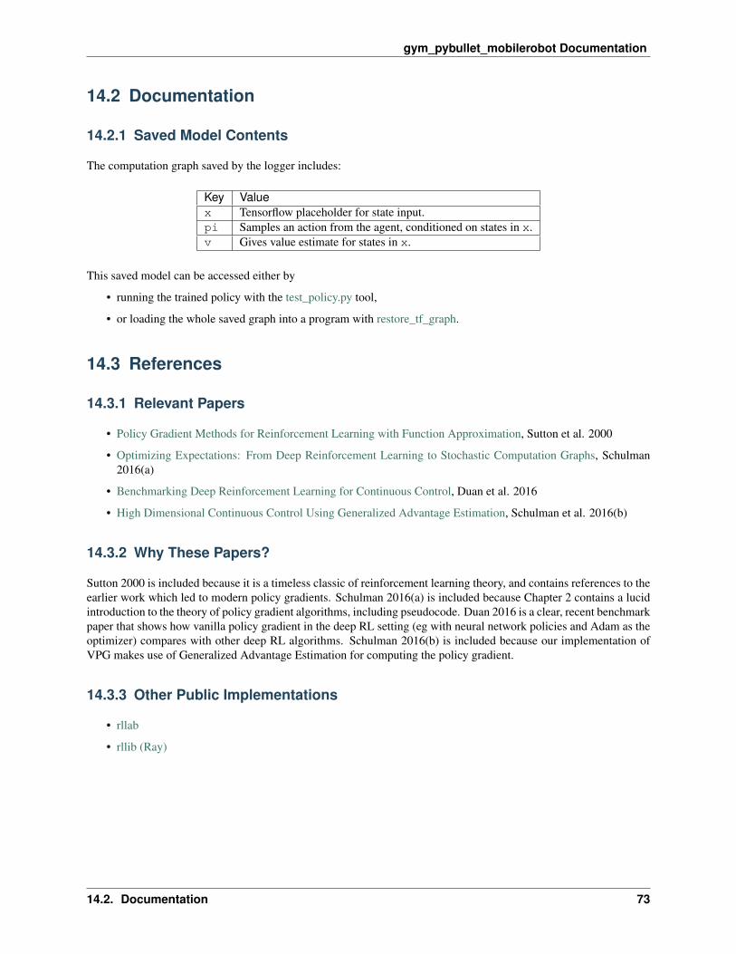
gym_pybullet_mobilerobot Documentation

14.2 Documentation

14.2.1 Saved Model Contents

The computation graph saved by the logger includes:

Key Valuex Tensorflow placeholder for state input.pi Samples an action from the agent, conditioned on states in x.v Gives value estimate for states in x.

This saved model can be accessed either by

• running the trained policy with the test_policy.py tool,

• or loading the whole saved graph into a program with restore_tf_graph.

14.3 References

14.3.1 Relevant Papers

• Policy Gradient Methods for Reinforcement Learning with Function Approximation, Sutton et al. 2000

• Optimizing Expectations: From Deep Reinforcement Learning to Stochastic Computation Graphs, Schulman2016(a)

• Benchmarking Deep Reinforcement Learning for Continuous Control, Duan et al. 2016

• High Dimensional Continuous Control Using Generalized Advantage Estimation, Schulman et al. 2016(b)

14.3.2 Why These Papers?

Sutton 2000 is included because it is a timeless classic of reinforcement learning theory, and contains references to theearlier work which led to modern policy gradients. Schulman 2016(a) is included because Chapter 2 contains a lucidintroduction to the theory of policy gradient algorithms, including pseudocode. Duan 2016 is a clear, recent benchmarkpaper that shows how vanilla policy gradient in the deep RL setting (eg with neural network policies and Adam as theoptimizer) compares with other deep RL algorithms. Schulman 2016(b) is included because our implementation ofVPG makes use of Generalized Advantage Estimation for computing the policy gradient.

14.3.3 Other Public Implementations

• rllab

• rllib (Ray)

14.2. Documentation 73

gym_pybullet_mobilerobot Documentation

74 Chapter 14. Vanilla Policy Gradient

CHAPTER 15

Trust Region Policy Optimization

Table of Contents

• Trust Region Policy Optimization

– Background

* Quick Facts

* Key Equations

* Exploration vs. Exploitation

* Pseudocode

– Documentation

* Saved Model Contents

– References

* Relevant Papers

* Why These Papers?

* Other Public Implementations

15.1 Background

(Previously: Background for VPG)

TRPO updates policies by taking the largest step possible to improve performance, while satisfying a special constrainton how close the new and old policies are allowed to be. The constraint is expressed in terms of KL-Divergence, ameasure of (something like, but not exactly) distance between probability distributions.

75

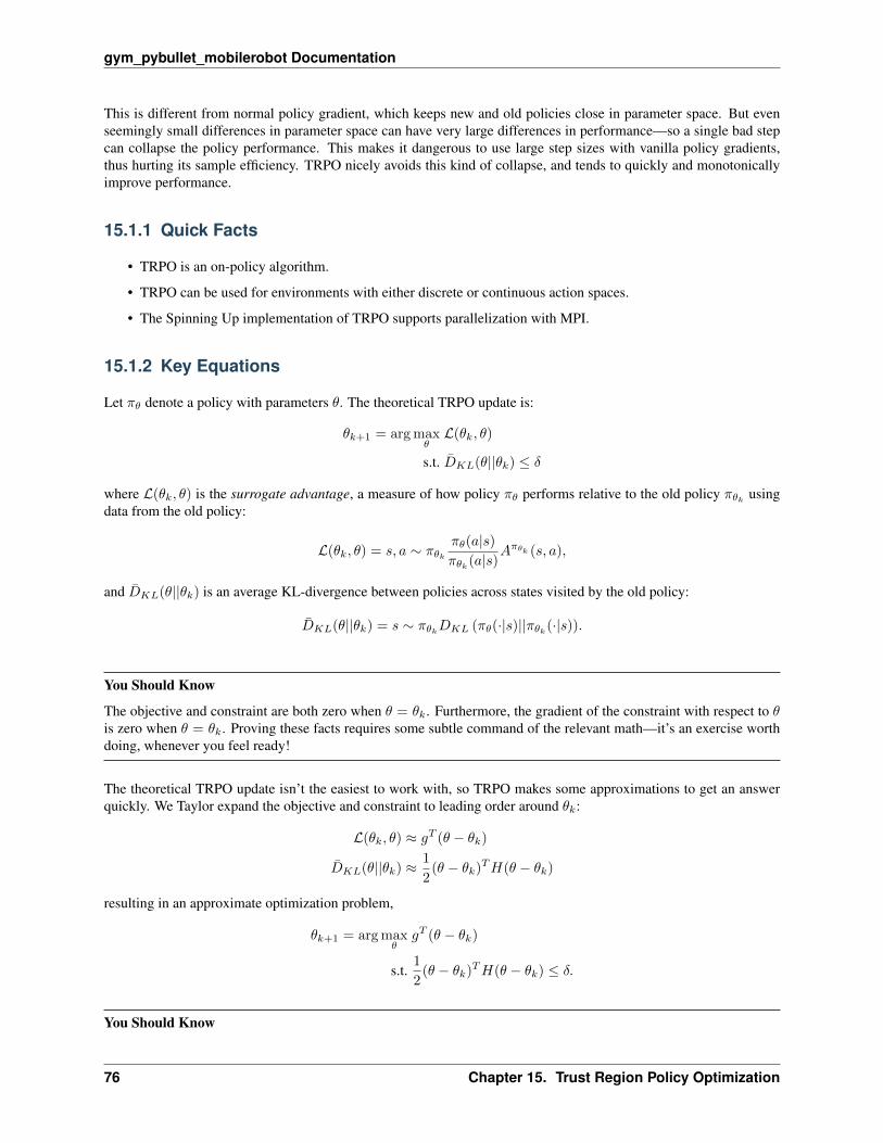
gym_pybullet_mobilerobot Documentation

This is different from normal policy gradient, which keeps new and old policies close in parameter space. But evenseemingly small differences in parameter space can have very large differences in performance—so a single bad stepcan collapse the policy performance. This makes it dangerous to use large step sizes with vanilla policy gradients,thus hurting its sample efficiency. TRPO nicely avoids this kind of collapse, and tends to quickly and monotonicallyimprove performance.

15.1.1 Quick Facts

• TRPO is an on-policy algorithm.

• TRPO can be used for environments with either discrete or continuous action spaces.

• The Spinning Up implementation of TRPO supports parallelization with MPI.

15.1.2 Key Equations

Let 𝜋𝜃 denote a policy with parameters 𝜃. The theoretical TRPO update is:

𝜃𝑘+1 = arg max𝜃ℒ(𝜃𝑘, 𝜃)

s.t. ��𝐾𝐿(𝜃||𝜃𝑘) ≤ 𝛿

where ℒ(𝜃𝑘, 𝜃) is the surrogate advantage, a measure of how policy 𝜋𝜃 performs relative to the old policy 𝜋𝜃𝑘 usingdata from the old policy:

ℒ(𝜃𝑘, 𝜃) = 𝑠, 𝑎 ∼ 𝜋𝜃𝑘𝜋𝜃(𝑎|𝑠)𝜋𝜃𝑘(𝑎|𝑠)

𝐴𝜋𝜃𝑘 (𝑠, 𝑎),

and ��𝐾𝐿(𝜃||𝜃𝑘) is an average KL-divergence between policies across states visited by the old policy:

��𝐾𝐿(𝜃||𝜃𝑘) = 𝑠 ∼ 𝜋𝜃𝑘𝐷𝐾𝐿 (𝜋𝜃(·|𝑠)||𝜋𝜃𝑘(·|𝑠)).

You Should Know

The objective and constraint are both zero when 𝜃 = 𝜃𝑘. Furthermore, the gradient of the constraint with respect to 𝜃is zero when 𝜃 = 𝜃𝑘. Proving these facts requires some subtle command of the relevant math—it’s an exercise worthdoing, whenever you feel ready!

The theoretical TRPO update isn’t the easiest to work with, so TRPO makes some approximations to get an answerquickly. We Taylor expand the objective and constraint to leading order around 𝜃𝑘:

ℒ(𝜃𝑘, 𝜃) ≈ 𝑔𝑇 (𝜃 − 𝜃𝑘)

��𝐾𝐿(𝜃||𝜃𝑘) ≈ 1

2(𝜃 − 𝜃𝑘)𝑇𝐻(𝜃 − 𝜃𝑘)

resulting in an approximate optimization problem,

𝜃𝑘+1 = arg max𝜃

𝑔𝑇 (𝜃 − 𝜃𝑘)

s.t.1

2(𝜃 − 𝜃𝑘)𝑇𝐻(𝜃 − 𝜃𝑘) ≤ 𝛿.

You Should Know

76 Chapter 15. Trust Region Policy Optimization

gym_pybullet_mobilerobot Documentation

By happy coincidence, the gradient 𝑔 of the surrogate advantage function with respect to 𝜃, evaluated at 𝜃 = 𝜃𝑘, isexactly equal to the policy gradient,∇𝜃𝐽(𝜋𝜃)! Try proving this, if you feel comfortable diving into the math.

This approximate problem can be analytically solved by the methods of Lagrangian duality1, yielding the solution:

𝜃𝑘+1 = 𝜃𝑘 +

√2𝛿

𝑔𝑇𝐻−1𝑔𝐻−1𝑔.

If we were to stop here, and just use this final result, the algorithm would be exactly calculating the Natural PolicyGradient. A problem is that, due to the approximation errors introduced by the Taylor expansion, this may not satisfythe KL constraint, or actually improve the surrogate advantage. TRPO adds a modification to this update rule: abacktracking line search,

𝜃𝑘+1 = 𝜃𝑘 + 𝛼𝑗

√2𝛿

𝑔𝑇𝐻−1𝑔𝐻−1𝑔,

where 𝛼 ∈ (0, 1) is the backtracking coefficient, and 𝑗 is the smallest nonnegative integer such that 𝜋𝜃𝑘+1satisfies the

KL constraint and produces a positive surrogate advantage.

Lastly: computing and storing the matrix inverse, 𝐻−1, is painfully expensive when dealing with neural networkpolicies with thousands or millions of parameters. TRPO sidesteps the issue by using the conjugate gradient algorithmto solve 𝐻𝑥 = 𝑔 for 𝑥 = 𝐻−1𝑔, requiring only a function which can compute the matrix-vector product 𝐻𝑥 insteadof computing and storing the whole matrix 𝐻 directly. This is not too hard to do: we set up a symbolic operation tocalculate

𝐻𝑥 = ∇𝜃((∇𝜃��𝐾𝐿(𝜃||𝜃𝑘)

)𝑇𝑥),

which gives us the correct output without computing the whole matrix.

15.1.3 Exploration vs. Exploitation

TRPO trains a stochastic policy in an on-policy way. This means that it explores by sampling actions according to thelatest version of its stochastic policy. The amount of randomness in action selection depends on both initial conditionsand the training procedure. Over the course of training, the policy typically becomes progressively less random, as theupdate rule encourages it to exploit rewards that it has already found. This may cause the policy to get trapped in localoptima.

15.1.4 Pseudocode

[H] Trust Region Policy Optimization [1] Input: initial policy parameters 𝜃0, initial value function parameters 𝜑0Hyperparameters: KL-divergence limit 𝛿, backtracking coefficient 𝛼, maximum number of backtracking steps 𝐾𝑘 = 0, 1, 2, ... Collect set of trajectories 𝒟𝑘 = {𝜏𝑖} by running policy 𝜋𝑘 = 𝜋(𝜃𝑘) in the environment. Computerewards-to-go ��𝑡. Compute advantage estimates, 𝐴𝑡 (using any method of advantage estimation) based on the currentvalue function 𝑉𝜑𝑘

. Estimate policy gradient as

𝑔𝑘 =1

|𝒟𝑘|∑𝜏∈𝒟𝑘

𝑇∑𝑡=0

∇𝜃 log 𝜋𝜃(𝑎𝑡|𝑠𝑡)|𝜃𝑘 𝐴𝑡.

Use the conjugate gradient algorithm to compute

��𝑘 ≈ ��−1𝑘 𝑔𝑘,

1 See Convex Optimization by Boyd and Vandenberghe, especially chapters 2 through 5.

15.1. Background 77

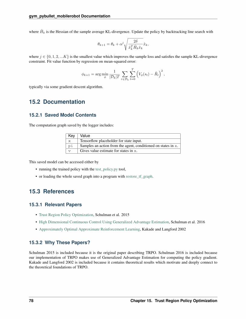
gym_pybullet_mobilerobot Documentation

where ��𝑘 is the Hessian of the sample average KL-divergence. Update the policy by backtracking line search with

𝜃𝑘+1 = 𝜃𝑘 + 𝛼𝑗

√2𝛿

��𝑇𝑘 ��𝑘��𝑘��𝑘,

where 𝑗 ∈ {0, 1, 2, ...𝐾} is the smallest value which improves the sample loss and satisfies the sample KL-divergenceconstraint. Fit value function by regression on mean-squared error:

𝜑𝑘+1 = arg min𝜑

1

|𝒟𝑘|𝑇∑𝜏∈𝒟𝑘

𝑇∑𝑡=0

(𝑉𝜑(𝑠𝑡)− ��𝑡

)2,

typically via some gradient descent algorithm.

15.2 Documentation

15.2.1 Saved Model Contents

The computation graph saved by the logger includes:

Key Valuex Tensorflow placeholder for state input.pi Samples an action from the agent, conditioned on states in x.v Gives value estimate for states in x.

This saved model can be accessed either by

• running the trained policy with the test_policy.py tool,

• or loading the whole saved graph into a program with restore_tf_graph.

15.3 References

15.3.1 Relevant Papers

• Trust Region Policy Optimization, Schulman et al. 2015

• High Dimensional Continuous Control Using Generalized Advantage Estimation, Schulman et al. 2016

• Approximately Optimal Approximate Reinforcement Learning, Kakade and Langford 2002

15.3.2 Why These Papers?

Schulman 2015 is included because it is the original paper describing TRPO. Schulman 2016 is included becauseour implementation of TRPO makes use of Generalized Advantage Estimation for computing the policy gradient.Kakade and Langford 2002 is included because it contains theoretical results which motivate and deeply connect tothe theoretical foundations of TRPO.

78 Chapter 15. Trust Region Policy Optimization

gym_pybullet_mobilerobot Documentation

15.3.3 Other Public Implementations

• Baselines

• ModularRL

• rllab

15.3. References 79

gym_pybullet_mobilerobot Documentation

80 Chapter 15. Trust Region Policy Optimization

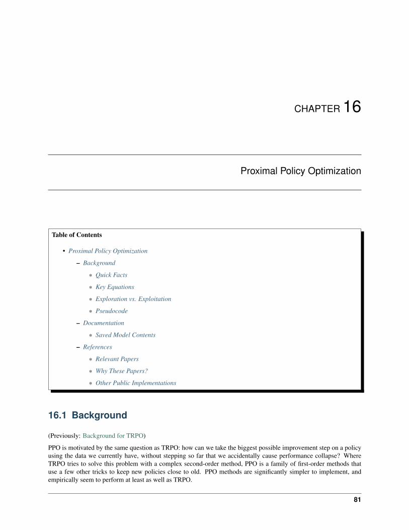
CHAPTER 16

Proximal Policy Optimization

Table of Contents

• Proximal Policy Optimization

– Background

* Quick Facts

* Key Equations

* Exploration vs. Exploitation

* Pseudocode

– Documentation

* Saved Model Contents

– References

* Relevant Papers

* Why These Papers?

* Other Public Implementations

16.1 Background

(Previously: Background for TRPO)

PPO is motivated by the same question as TRPO: how can we take the biggest possible improvement step on a policyusing the data we currently have, without stepping so far that we accidentally cause performance collapse? WhereTRPO tries to solve this problem with a complex second-order method, PPO is a family of first-order methods thatuse a few other tricks to keep new policies close to old. PPO methods are significantly simpler to implement, andempirically seem to perform at least as well as TRPO.

81

gym_pybullet_mobilerobot Documentation

There are two primary variants of PPO: PPO-Penalty and PPO-Clip.

PPO-Penalty approximately solves a KL-constrained update like TRPO, but penalizes the KL-divergence in the ob-jective function instead of making it a hard constraint, and automatically adjusts the penalty coefficient over the courseof training so that it’s scaled appropriately.

PPO-Clip doesn’t have a KL-divergence term in the objective and doesn’t have a constraint at all. Instead relies onspecialized clipping in the objective function to remove incentives for the new policy to get far from the old policy.

Here, we’ll focus only on PPO-Clip (the primary variant used at OpenAI).

16.1.1 Quick Facts

• PPO is an on-policy algorithm.

• PPO can be used for environments with either discrete or continuous action spaces.

• The Spinning Up implementation of PPO supports parallelization with MPI.

16.1.2 Key Equations

PPO-clip updates policies via

𝜃𝑘+1 = arg max𝜃

E𝑠,𝑎∼𝜋𝜃𝑘

[𝐿(𝑠, 𝑎, 𝜃𝑘, 𝜃)] ,

typically taking multiple steps of (usually minibatch) SGD to maximize the objective. Here 𝐿 is given by

𝐿(𝑠, 𝑎, 𝜃𝑘, 𝜃) = min

(𝜋𝜃(𝑎|𝑠)𝜋𝜃𝑘(𝑎|𝑠)

𝐴𝜋𝜃𝑘 (𝑠, 𝑎), clip(𝜋𝜃(𝑎|𝑠)𝜋𝜃𝑘(𝑎|𝑠)

, 1− 𝜖, 1 + 𝜖

)𝐴𝜋𝜃𝑘 (𝑠, 𝑎)

),

in which 𝜖 is a (small) hyperparameter which roughly says how far away the new policy is allowed to go from the old.

This is a pretty complex expression, and it’s hard to tell at first glance what it’s doing, or how it helps keep the newpolicy close to the old policy. As it turns out, there’s a considerably simplified version1 of this objective which is a biteasier to grapple with (and is also the version we implement in our code):

𝐿(𝑠, 𝑎, 𝜃𝑘, 𝜃) = min

(𝜋𝜃(𝑎|𝑠)𝜋𝜃𝑘(𝑎|𝑠)

𝐴𝜋𝜃𝑘 (𝑠, 𝑎), 𝑔(𝜖, 𝐴𝜋𝜃𝑘 (𝑠, 𝑎))

),

where

𝑔(𝜖, 𝐴) =

{(1 + 𝜖)𝐴 𝐴 ≥ 0(1− 𝜖)𝐴 𝐴 < 0.

To figure out what intuition to take away from this, let’s look at a single state-action pair (𝑠, 𝑎), and think of cases.

Advantage is positive: Suppose the advantage for that state-action pair is positive, in which case its contribution tothe objective reduces to

𝐿(𝑠, 𝑎, 𝜃𝑘, 𝜃) = min

(𝜋𝜃(𝑎|𝑠)𝜋𝜃𝑘(𝑎|𝑠)

, (1 + 𝜖)

)𝐴𝜋𝜃𝑘 (𝑠, 𝑎).

Because the advantage is positive, the objective will increase if the action becomes more likely—that is, if 𝜋𝜃(𝑎|𝑠)increases. But the min in this term puts a limit to how much the objective can increase. Once 𝜋𝜃(𝑎|𝑠) > (1+𝜖)𝜋𝜃𝑘(𝑎|𝑠),the min kicks in and this term hits a ceiling of (1 + 𝜖)𝐴𝜋𝜃𝑘 (𝑠, 𝑎). Thus: the new policy does not benefit by going faraway from the old policy.

1 See this note for a derivation of the simplified form of the PPO-Clip objective.

82 Chapter 16. Proximal Policy Optimization

gym_pybullet_mobilerobot Documentation

Advantage is negative: Suppose the advantage for that state-action pair is negative, in which case its contribution tothe objective reduces to

𝐿(𝑠, 𝑎, 𝜃𝑘, 𝜃) = max

(𝜋𝜃(𝑎|𝑠)𝜋𝜃𝑘(𝑎|𝑠)

, (1− 𝜖))𝐴𝜋𝜃𝑘 (𝑠, 𝑎).

Because the advantage is negative, the objective will increase if the action becomes less likely—that is, if 𝜋𝜃(𝑎|𝑠)decreases. But the max in this term puts a limit to how much the objective can increase. Once 𝜋𝜃(𝑎|𝑠) < (1 −𝜖)𝜋𝜃𝑘(𝑎|𝑠), the max kicks in and this term hits a ceiling of (1 − 𝜖)𝐴𝜋𝜃𝑘 (𝑠, 𝑎). Thus, again: the new policy does notbenefit by going far away from the old policy.

What we have seen so far is that clipping serves as a regularizer by removing incentives for the policy to changedramatically, and the hyperparameter 𝜖 corresponds to how far away the new policy can go from the old while stillprofiting the objective.

You Should Know

While this kind of clipping goes a long way towards ensuring reasonable policy updates, it is still possible to endup with a new policy which is too far from the old policy, and there are a bunch of tricks used by different PPOimplementations to stave this off. In our implementation here, we use a particularly simple method: early stopping. Ifthe mean KL-divergence of the new policy from the old grows beyond a threshold, we stop taking gradient steps.

When you feel comfortable with the basic math and implementation details, it’s worth checking out other implemen-tations to see how they handle this issue!

16.1.3 Exploration vs. Exploitation

PPO trains a stochastic policy in an on-policy way. This means that it explores by sampling actions according to thelatest version of its stochastic policy. The amount of randomness in action selection depends on both initial conditionsand the training procedure. Over the course of training, the policy typically becomes progressively less random, as theupdate rule encourages it to exploit rewards that it has already found. This may cause the policy to get trapped in localoptima.

16.1.4 Pseudocode

[H] PPO-Clip [1] Input: initial policy parameters 𝜃0, initial value function parameters 𝜑0 𝑘 = 0, 1, 2, ... Collect setof trajectories 𝒟𝑘 = {𝜏𝑖} by running policy 𝜋𝑘 = 𝜋(𝜃𝑘) in the environment. Compute rewards-to-go ��𝑡. Computeadvantage estimates, 𝐴𝑡 (using any method of advantage estimation) based on the current value function 𝑉𝜑𝑘

. Updatethe policy by maximizing the PPO-Clip objective:

𝜃𝑘+1 = arg max𝜃

1

|𝒟𝑘|𝑇∑𝜏∈𝒟𝑘

𝑇∑𝑡=0

min

(𝜋𝜃(𝑎𝑡|𝑠𝑡)𝜋𝜃𝑘(𝑎𝑡|𝑠𝑡)

𝐴𝜋𝜃𝑘 (𝑠𝑡, 𝑎𝑡), 𝑔(𝜖, 𝐴𝜋𝜃𝑘 (𝑠𝑡, 𝑎𝑡))

),

typically via stochastic gradient ascent with Adam. Fit value function by regression on mean-squared error:

𝜑𝑘+1 = arg min𝜑

1

|𝒟𝑘|𝑇∑𝜏∈𝒟𝑘

𝑇∑𝑡=0

(𝑉𝜑(𝑠𝑡)− ��𝑡

)2,

typically via some gradient descent algorithm.

16.1. Background 83

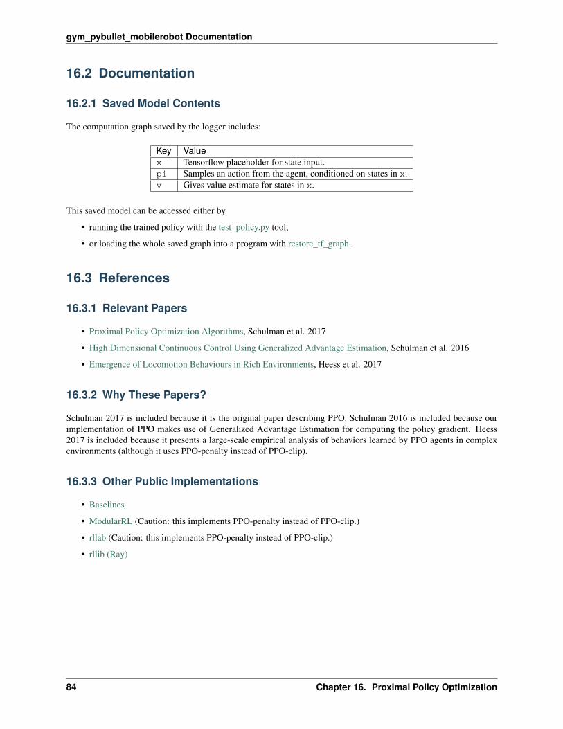
gym_pybullet_mobilerobot Documentation

16.2 Documentation

16.2.1 Saved Model Contents

The computation graph saved by the logger includes:

Key Valuex Tensorflow placeholder for state input.pi Samples an action from the agent, conditioned on states in x.v Gives value estimate for states in x.

This saved model can be accessed either by

• running the trained policy with the test_policy.py tool,

• or loading the whole saved graph into a program with restore_tf_graph.

16.3 References

16.3.1 Relevant Papers

• Proximal Policy Optimization Algorithms, Schulman et al. 2017

• High Dimensional Continuous Control Using Generalized Advantage Estimation, Schulman et al. 2016

• Emergence of Locomotion Behaviours in Rich Environments, Heess et al. 2017

16.3.2 Why These Papers?

Schulman 2017 is included because it is the original paper describing PPO. Schulman 2016 is included because ourimplementation of PPO makes use of Generalized Advantage Estimation for computing the policy gradient. Heess2017 is included because it presents a large-scale empirical analysis of behaviors learned by PPO agents in complexenvironments (although it uses PPO-penalty instead of PPO-clip).

16.3.3 Other Public Implementations

• Baselines

• ModularRL (Caution: this implements PPO-penalty instead of PPO-clip.)

• rllab (Caution: this implements PPO-penalty instead of PPO-clip.)

• rllib (Ray)

84 Chapter 16. Proximal Policy Optimization

CHAPTER 17

Deep Deterministic Policy Gradient

Table of Contents

• Deep Deterministic Policy Gradient

– Background

* Quick Facts

* Key Equations

· The Q-Learning Side of DDPG

· The Policy Learning Side of DDPG

* Exploration vs. Exploitation

* Pseudocode

– Documentation

* Saved Model Contents

– References

* Relevant Papers

* Why These Papers?

* Other Public Implementations

17.1 Background

(Previously: Introduction to RL Part 1: The Optimal Q-Function and the Optimal Action)

Deep Deterministic Policy Gradient (DDPG) is an algorithm which concurrently learns a Q-function and a policy. Ituses off-policy data and the Bellman equation to learn the Q-function, and uses the Q-function to learn the policy.

85

gym_pybullet_mobilerobot Documentation

This approach is closely connected to Q-learning, and is motivated the same way: if you know the optimal action-valuefunction 𝑄*(𝑠, 𝑎), then in any given state, the optimal action 𝑎*(𝑠) can be found by solving

𝑎*(𝑠) = arg max𝑎

𝑄*(𝑠, 𝑎).

DDPG interleaves learning an approximator to 𝑄*(𝑠, 𝑎) with learning an approximator to 𝑎*(𝑠), and it does so in away which is specifically adapted for environments with continuous action spaces. But what does it mean that DDPGis adapted specifically for environments with continuous action spaces? It relates to how we compute the max overactions in max𝑎𝑄

*(𝑠, 𝑎).

When there are a finite number of discrete actions, the max poses no problem, because we can just compute theQ-values for each action separately and directly compare them. (This also immediately gives us the action whichmaximizes the Q-value.) But when the action space is continuous, we can’t exhaustively evaluate the space, andsolving the optimization problem is highly non-trivial. Using a normal optimization algorithm would make calculatingmax𝑎𝑄

*(𝑠, 𝑎) a painfully expensive subroutine. And since it would need to be run every time the agent wants to takean action in the environment, this is unacceptable.

Because the action space is continuous, the function𝑄*(𝑠, 𝑎) is presumed to be differentiable with respect to the actionargument. This allows us to set up an efficient, gradient-based learning rule for a policy 𝜇(𝑠) which exploits that fact.Then, instead of running an expensive optimization subroutine each time we wish to compute max𝑎𝑄(𝑠, 𝑎), we canapproximate it with max𝑎𝑄(𝑠, 𝑎) ≈ 𝑄(𝑠, 𝜇(𝑠)). See the Key Equations section details.

17.1.1 Quick Facts

• DDPG is an off-policy algorithm.

• DDPG can only be used for environments with continuous action spaces.

• DDPG can be thought of as being deep Q-learning for continuous action spaces.

• The Spinning Up implementation of DDPG does not support parallelization.

17.1.2 Key Equations

Here, we’ll explain the math behind the two parts of DDPG: learning a Q function, and learning a policy.

The Q-Learning Side of DDPG

First, let’s recap the Bellman equation describing the optimal action-value function, 𝑄*(𝑠, 𝑎). It’s given by

𝑄*(𝑠, 𝑎) = E𝑠′∼𝑃

[𝑟(𝑠, 𝑎) + 𝛾max

𝑎′𝑄*(𝑠′, 𝑎′)

]where 𝑠′ ∼ 𝑃 is shorthand for saying that the next state, 𝑠′, is sampled by the environment from a distribution 𝑃 (·|𝑠, 𝑎).

This Bellman equation is the starting point for learning an approximator to 𝑄*(𝑠, 𝑎). Suppose the approximator is aneural network 𝑄𝜑(𝑠, 𝑎), with parameters 𝜑, and that we have collected a set 𝒟 of transitions (𝑠, 𝑎, 𝑟, 𝑠′, 𝑑) (where 𝑑indicates whether state 𝑠′ is terminal). We can set up a mean-squared Bellman error (MSBE) function, which tellsus roughly how closely 𝑄𝜑 comes to satisfying the Bellman equation:

𝐿(𝜑,𝒟) = E(𝑠,𝑎,𝑟,𝑠′,𝑑)∼𝒟

⎡⎣(𝑄𝜑(𝑠, 𝑎)−(𝑟 + 𝛾(1− 𝑑) max

𝑎′𝑄𝜑(𝑠′, 𝑎′)

))2⎤⎦

Here, in evaluating (1− 𝑑), we’ve used a Python convention of evaluating True to 1 and False to zero. Thus, whend==True—which is to say, when 𝑠′ is a terminal state—the Q-function should show that the agent gets no additionalrewards after the current state. (This choice of notation corresponds to what we later implement in code.)

86 Chapter 17. Deep Deterministic Policy Gradient

gym_pybullet_mobilerobot Documentation

Q-learning algorithms for function approximators, such as DQN (and all its variants) and DDPG, are largely based onminimizing this MSBE loss function. There are two main tricks employed by all of them which are worth describing,and then a specific detail for DDPG.

Trick One: Replay Buffers. All standard algorithms for training a deep neural network to approximate 𝑄*(𝑠, 𝑎)make use of an experience replay buffer. This is the set 𝒟 of previous experiences. In order for the algorithm to havestable behavior, the replay buffer should be large enough to contain a wide range of experiences, but it may not alwaysbe good to keep everything. If you only use the very-most recent data, you will overfit to that and things will break; ifyou use too much experience, you may slow down your learning. This may take some tuning to get right.

You Should Know

We’ve mentioned that DDPG is an off-policy algorithm: this is as good a point as any to highlight why and how.Observe that the replay buffer should contain old experiences, even though they might have been obtained using anoutdated policy. Why are we able to use these at all? The reason is that the Bellman equation doesn’t care whichtransition tuples are used, or how the actions were selected, or what happens after a given transition, because theoptimal Q-function should satisfy the Bellman equation for all possible transitions. So any transitions that we’ve everexperienced are fair game when trying to fit a Q-function approximator via MSBE minimization.

Trick Two: Target Networks. Q-learning algorithms make use of target networks. The term

𝑟 + 𝛾(1− 𝑑) max𝑎′

𝑄𝜑(𝑠′, 𝑎′)

is called the target, because when we minimize the MSBE loss, we are trying to make the Q-function be more likethis target. Problematically, the target depends on the same parameters we are trying to train: 𝜑. This makes MSBEminimization unstable. The solution is to use a set of parameters which comes close to 𝜑, but with a time delay—thatis to say, a second network, called the target network, which lags the first. The parameters of the target network aredenoted 𝜑targ.

In DQN-based algorithms, the target network is just copied over from the main network every some-fixed-number ofsteps. In DDPG-style algorithms, the target network is updated once per main network update by polyak averaging:

𝜑targ ← 𝜌𝜑targ + (1− 𝜌)𝜑,

where 𝜌 is a hyperparameter between 0 and 1 (usually close to 1). (This hyperparameter is called polyak in ourcode).

DDPG Detail: Calculating the Max Over Actions in the Target. As mentioned earlier: computing the maximumover actions in the target is a challenge in continuous action spaces. DDPG deals with this by using a target policynetwork to compute an action which approximately maximizes 𝑄𝜑targ . The target policy network is found the sameway as the target Q-function: by polyak averaging the policy parameters over the course of training.

Putting it all together, Q-learning in DDPG is performed by minimizing the following MSBE loss with stochasticgradient descent:

𝐿(𝜑,𝒟) = E(𝑠,𝑎,𝑟,𝑠′,𝑑)∼𝒟

⎡⎣(𝑄𝜑(𝑠, 𝑎)−(𝑟 + 𝛾(1− 𝑑)𝑄𝜑targ(𝑠

′, 𝜇𝜃targ(𝑠′))))2

⎤⎦ ,where 𝜇𝜃targ is the target policy.

The Policy Learning Side of DDPG

Policy learning in DDPG is fairly simple. We want to learn a deterministic policy 𝜇𝜃(𝑠) which gives the action thatmaximizes 𝑄𝜑(𝑠, 𝑎). Because the action space is continuous, and we assume the Q-function is differentiable withrespect to action, we can just perform gradient ascent (with respect to policy parameters only) to solve

max𝜃

E𝑠∼𝒟

[𝑄𝜑(𝑠, 𝜇𝜃(𝑠))] .

17.1. Background 87

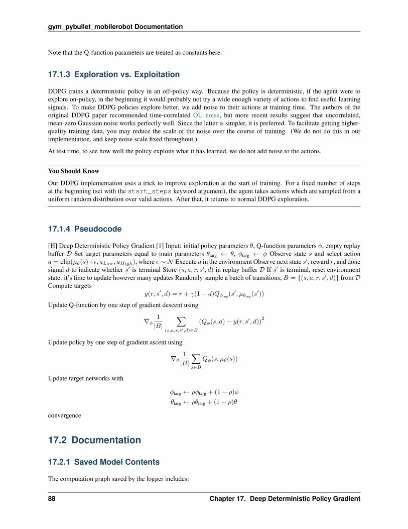
gym_pybullet_mobilerobot Documentation

Note that the Q-function parameters are treated as constants here.

17.1.3 Exploration vs. Exploitation

DDPG trains a deterministic policy in an off-policy way. Because the policy is deterministic, if the agent were toexplore on-policy, in the beginning it would probably not try a wide enough variety of actions to find useful learningsignals. To make DDPG policies explore better, we add noise to their actions at training time. The authors of theoriginal DDPG paper recommended time-correlated OU noise, but more recent results suggest that uncorrelated,mean-zero Gaussian noise works perfectly well. Since the latter is simpler, it is preferred. To facilitate getting higher-quality training data, you may reduce the scale of the noise over the course of training. (We do not do this in ourimplementation, and keep noise scale fixed throughout.)

At test time, to see how well the policy exploits what it has learned, we do not add noise to the actions.

You Should Know

Our DDPG implementation uses a trick to improve exploration at the start of training. For a fixed number of stepsat the beginning (set with the start_steps keyword argument), the agent takes actions which are sampled from auniform random distribution over valid actions. After that, it returns to normal DDPG exploration.

17.1.4 Pseudocode

[H] Deep Deterministic Policy Gradient [1] Input: initial policy parameters 𝜃, Q-function parameters 𝜑, empty replaybuffer 𝒟 Set target parameters equal to main parameters 𝜃targ ← 𝜃, 𝜑targ ← 𝜑 Observe state 𝑠 and select action𝑎 = clip(𝜇𝜃(𝑠)+𝜖, 𝑎𝐿𝑜𝑤, 𝑎𝐻𝑖𝑔ℎ), where 𝜖 ∼ 𝒩 Execute 𝑎 in the environment Observe next state 𝑠′, reward 𝑟, and donesignal 𝑑 to indicate whether 𝑠′ is terminal Store (𝑠, 𝑎, 𝑟, 𝑠′, 𝑑) in replay buffer 𝒟 If 𝑠′ is terminal, reset environmentstate. it’s time to update however many updates Randomly sample a batch of transitions, 𝐵 = {(𝑠, 𝑎, 𝑟, 𝑠′, 𝑑)} from 𝒟Compute targets

𝑦(𝑟, 𝑠′, 𝑑) = 𝑟 + 𝛾(1− 𝑑)𝑄𝜑targ(𝑠′, 𝜇𝜃targ(𝑠

′))

Update Q-function by one step of gradient descent using

∇𝜑1

|𝐵|∑

(𝑠,𝑎,𝑟,𝑠′,𝑑)∈𝐵

(𝑄𝜑(𝑠, 𝑎)− 𝑦(𝑟, 𝑠′, 𝑑))2

Update policy by one step of gradient ascent using

∇𝜃1

|𝐵|∑𝑠∈𝐵

𝑄𝜑(𝑠, 𝜇𝜃(𝑠))

Update target networks with

𝜑targ ← 𝜌𝜑targ + (1− 𝜌)𝜑

𝜃targ ← 𝜌𝜃targ + (1− 𝜌)𝜃

convergence

17.2 Documentation

17.2.1 Saved Model Contents

The computation graph saved by the logger includes:

88 Chapter 17. Deep Deterministic Policy Gradient

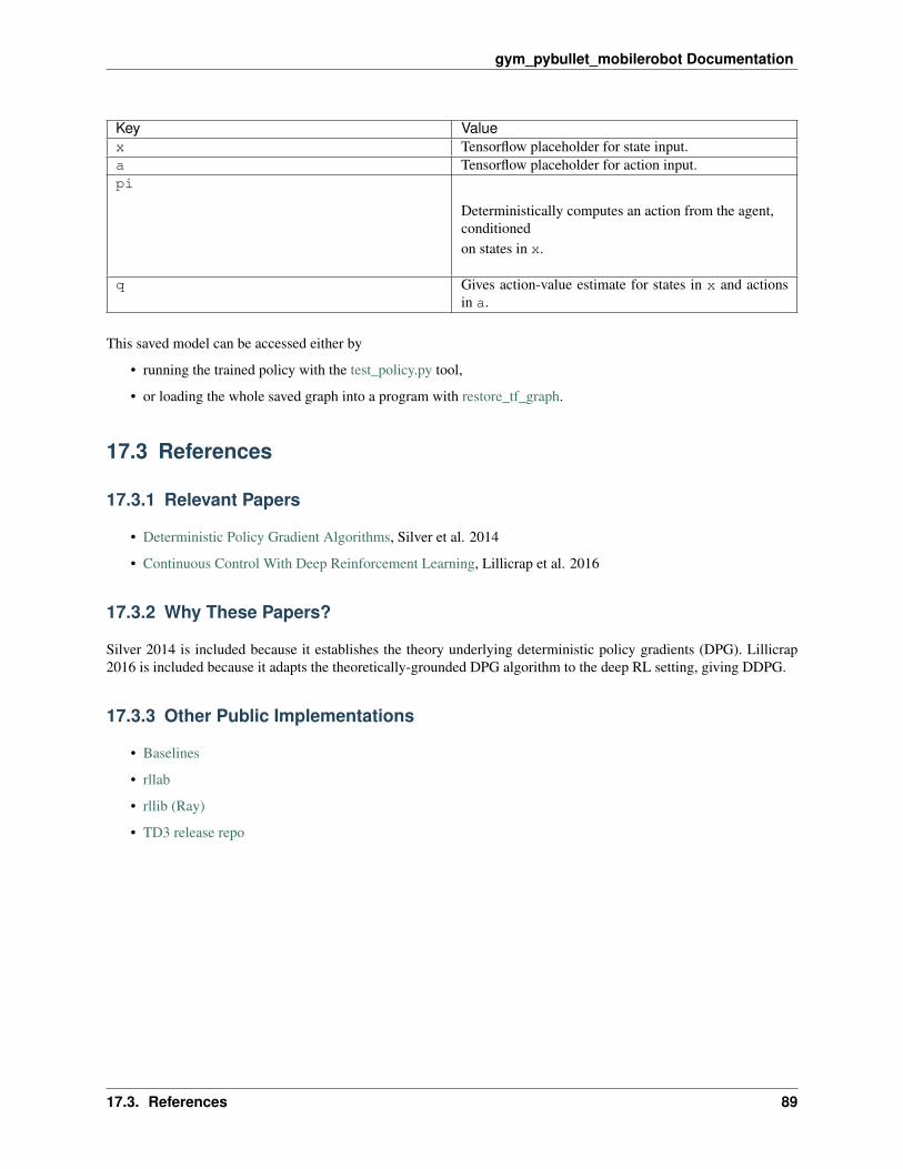
gym_pybullet_mobilerobot Documentation

Key Valuex Tensorflow placeholder for state input.a Tensorflow placeholder for action input.pi

Deterministically computes an action from the agent,conditionedon states in x.

q Gives action-value estimate for states in x and actionsin a.

This saved model can be accessed either by

• running the trained policy with the test_policy.py tool,

• or loading the whole saved graph into a program with restore_tf_graph.

17.3 References

17.3.1 Relevant Papers

• Deterministic Policy Gradient Algorithms, Silver et al. 2014

• Continuous Control With Deep Reinforcement Learning, Lillicrap et al. 2016

17.3.2 Why These Papers?

Silver 2014 is included because it establishes the theory underlying deterministic policy gradients (DPG). Lillicrap2016 is included because it adapts the theoretically-grounded DPG algorithm to the deep RL setting, giving DDPG.

17.3.3 Other Public Implementations

• Baselines

• rllab

• rllib (Ray)

• TD3 release repo

17.3. References 89

gym_pybullet_mobilerobot Documentation

90 Chapter 17. Deep Deterministic Policy Gradient

CHAPTER 18

Twin Delayed DDPG

Table of Contents

• Twin Delayed DDPG

– Background

* Quick Facts

* Key Equations

* Exploration vs. Exploitation

* Pseudocode

– Documentation

* Saved Model Contents

– References

* Relevant Papers

* Other Public Implementations

18.1 Background

(Previously: Background for DDPG)

While DDPG can achieve great performance sometimes, it is frequently brittle with respect to hyperparameters andother kinds of tuning. A common failure mode for DDPG is that the learned Q-function begins to dramaticallyoverestimate Q-values, which then leads to the policy breaking, because it exploits the errors in the Q-function. TwinDelayed DDPG (TD3) is an algorithm which addresses this issue by introducing three critical tricks:

Trick One: Clipped Double-Q Learning. TD3 learns two Q-functions instead of one (hence “twin”), and uses thesmaller of the two Q-values to form the targets in the Bellman error loss functions.

91

gym_pybullet_mobilerobot Documentation

Trick Two: “Delayed” Policy Updates. TD3 updates the policy (and target networks) less frequently than the Q-function. The paper recommends one policy update for every two Q-function updates.

Trick Three: Target Policy Smoothing. TD3 adds noise to the target action, to make it harder for the policy to exploitQ-function errors by smoothing out Q along changes in action.

Together, these three tricks result in substantially improved performance over baseline DDPG.

18.1.1 Quick Facts

• TD3 is an off-policy algorithm.

• TD3 can only be used for environments with continuous action spaces.

• The Spinning Up implementation of TD3 does not support parallelization.

18.1.2 Key Equations

TD3 concurrently learns two Q-functions, 𝑄𝜑1and 𝑄𝜑2

, by mean square Bellman error minimization, in almost thesame way that DDPG learns its single Q-function. To show exactly how TD3 does this and how it differs from normalDDPG, we’ll work from the innermost part of the loss function outwards.

First: target policy smoothing. Actions used to form the Q-learning target are based on the target policy, 𝜇𝜃targ , butwith clipped noise added on each dimension of the action. After adding the clipped noise, the target action is thenclipped to lie in the valid action range (all valid actions, 𝑎, satisfy 𝑎𝐿𝑜𝑤 ≤ 𝑎 ≤ 𝑎𝐻𝑖𝑔ℎ). The target actions are thus:

𝑎′(𝑠′) = clip(𝜇𝜃targ(𝑠

′) + clip(𝜖,−𝑐, 𝑐), 𝑎𝐿𝑜𝑤, 𝑎𝐻𝑖𝑔ℎ), 𝜖 ∼ 𝒩 (0, 𝜎)

Target policy smoothing essentially serves as a regularizer for the algorithm. It addresses a particular failure mode thatcan happen in DDPG: if the Q-function approximator develops an incorrect sharp peak for some actions, the policywill quickly exploit that peak and then have brittle or incorrect behavior. This can be averted by smoothing out theQ-function over similar actions, which target policy smoothing is designed to do.

Next: clipped double-Q learning. Both Q-functions use a single target, calculated using whichever of the two Q-functions gives a smaller target value:

𝑦(𝑟, 𝑠′, 𝑑) = 𝑟 + 𝛾(1− 𝑑) min𝑖=1,2

𝑄𝜑𝑖,targ(𝑠′, 𝑎′(𝑠′)),

and then both are learned by regressing to this target:

𝐿(𝜑1,𝒟) = (𝑠, 𝑎, 𝑟, 𝑠′, 𝑑) ∼ 𝒟

(𝑄𝜑1(𝑠, 𝑎)− 𝑦(𝑟, 𝑠′, 𝑑)

)2

,

𝐿(𝜑2,𝒟) = (𝑠, 𝑎, 𝑟, 𝑠′, 𝑑) ∼ 𝒟

(𝑄𝜑2

(𝑠, 𝑎)− 𝑦(𝑟, 𝑠′, 𝑑)

)2

.

Using the smaller Q-value for the target, and regressing towards that, helps fend off overestimation in the Q-function.

Lastly: the policy is learned just by maximizing 𝑄𝜑1 :

max𝜃

E𝑠∼𝒟

[𝑄𝜑1(𝑠, 𝜇𝜃(𝑠))] ,

which is pretty much unchanged from DDPG. However, in TD3, the policy is updated less frequently than the Q-functions are. This helps damp the volatility that normally arises in DDPG because of how a policy update changesthe target.

92 Chapter 18. Twin Delayed DDPG

gym_pybullet_mobilerobot Documentation

18.1.3 Exploration vs. Exploitation

TD3 trains a deterministic policy in an off-policy way. Because the policy is deterministic, if the agent were to exploreon-policy, in the beginning it would probably not try a wide enough variety of actions to find useful learning signals.To make TD3 policies explore better, we add noise to their actions at training time, typically uncorrelated mean-zeroGaussian noise. To facilitate getting higher-quality training data, you may reduce the scale of the noise over the courseof training. (We do not do this in our implementation, and keep noise scale fixed throughout.)

At test time, to see how well the policy exploits what it has learned, we do not add noise to the actions.

You Should Know

Our TD3 implementation uses a trick to improve exploration at the start of training. For a fixed number of steps atthe beginning (set with the start_steps keyword argument), the agent takes actions which are sampled from auniform random distribution over valid actions. After that, it returns to normal TD3 exploration.

18.1.4 Pseudocode

[H] Twin Delayed DDPG [1] Input: initial policy parameters 𝜃, Q-function parameters 𝜑1, 𝜑2, empty replay buffer𝒟 Set target parameters equal to main parameters 𝜃targ ← 𝜃, 𝜑targ,1 ← 𝜑1, 𝜑targ,2 ← 𝜑2 Observe state 𝑠 and selectaction 𝑎 = clip(𝜇𝜃(𝑠) + 𝜖, 𝑎𝐿𝑜𝑤, 𝑎𝐻𝑖𝑔ℎ), where 𝜖 ∼ 𝒩 Execute 𝑎 in the environment Observe next state 𝑠′, reward𝑟, and done signal 𝑑 to indicate whether 𝑠′ is terminal Store (𝑠, 𝑎, 𝑟, 𝑠′, 𝑑) in replay buffer 𝒟 If 𝑠′ is terminal, resetenvironment state. it’s time to update 𝑗 in range(however many updates) Randomly sample a batch of transitions,𝐵 = {(𝑠, 𝑎, 𝑟, 𝑠′, 𝑑)} from 𝒟 Compute target actions

𝑎′(𝑠′) = clip(𝜇𝜃targ(𝑠

′) + clip(𝜖,−𝑐, 𝑐), 𝑎𝐿𝑜𝑤, 𝑎𝐻𝑖𝑔ℎ), 𝜖 ∼ 𝒩 (0, 𝜎)

Compute targets𝑦(𝑟, 𝑠′, 𝑑) = 𝑟 + 𝛾(1− 𝑑) min

𝑖=1,2𝑄𝜑targ,𝑖(𝑠

′, 𝑎′(𝑠′))

Update Q-functions by one step of gradient descent using

∇𝜑𝑖

1

|𝐵|∑

(𝑠,𝑎,𝑟,𝑠′,𝑑)∈𝐵

(𝑄𝜑,𝑖(𝑠, 𝑎)− 𝑦(𝑟, 𝑠′, 𝑑))2 for 𝑖 = 1, 2

𝑗 mod policy_delay = 0 Update policy by one step of gradient ascent using

∇𝜃1

|𝐵|∑𝑠∈𝐵

𝑄𝜑,1(𝑠, 𝜇𝜃(𝑠))

Update target networks with

𝜑targ,𝑖 ← 𝜌𝜑targ,𝑖 + (1− 𝜌)𝜑𝑖 for 𝑖 = 1, 2

𝜃targ ← 𝜌𝜃targ + (1− 𝜌)𝜃

convergence

18.2 Documentation

18.2.1 Saved Model Contents

The computation graph saved by the logger includes:

18.2. Documentation 93

gym_pybullet_mobilerobot Documentation

Key Valuex Tensorflow placeholder for state input.a Tensorflow placeholder for action input.pi

Deterministically computes an action from the agent,conditionedon states in x.

q1 Gives one action-value estimate for states in x and ac-tions in a.

q2 Gives the other action-value estimate for states in x andactions in a.

This saved model can be accessed either by

• running the trained policy with the test_policy.py tool,

• or loading the whole saved graph into a program with restore_tf_graph.

18.3 References

18.3.1 Relevant Papers

• Addressing Function Approximation Error in Actor-Critic Methods, Fujimoto et al, 2018

18.3.2 Other Public Implementations

• TD3 release repo

94 Chapter 18. Twin Delayed DDPG

CHAPTER 19

Soft Actor-Critic

Table of Contents

• Soft Actor-Critic

– Background

* Quick Facts

* Key Equations

· Entropy-Regularized Reinforcement Learning

· Soft Actor-Critic

* Exploration vs. Exploitation

* Pseudocode

– Documentation

* Saved Model Contents

– References

* Relevant Papers

* Other Public Implementations

19.1 Background

(Previously: Background for TD3)

Soft Actor Critic (SAC) is an algorithm which optimizes a stochastic policy in an off-policy way, forming a bridgebetween stochastic policy optimization and DDPG-style approaches. It isn’t a direct successor to TD3 (having been

95

gym_pybullet_mobilerobot Documentation

published roughly concurrently), but it incorporates the clipped double-Q trick, and due to the inherent stochasticityof the policy in SAC, it also winds up benefiting from something like target policy smoothing.

A central feature of SAC is entropy regularization. The policy is trained to maximize a trade-off between expectedreturn and entropy, a measure of randomness in the policy. This has a close connection to the exploration-exploitationtrade-off: increasing entropy results in more exploration, which can accelerate learning later on. It can also preventthe policy from prematurely converging to a bad local optimum.

19.1.1 Quick Facts

• SAC is an off-policy algorithm.

• The version of SAC implemented here can only be used for environments with continuous action spaces.

• An alternate version of SAC, which slightly changes the policy update rule, can be implemented to handlediscrete action spaces.

• The Spinning Up implementation of SAC does not support parallelization.

19.1.2 Key Equations

To explain Soft Actor Critic, we first have to introduce the entropy-regularized reinforcement learning setting. Inentropy-regularized RL, there are slightly-different equations for value functions.

Entropy-Regularized Reinforcement Learning

Entropy is a quantity which, roughly speaking, says how random a random variable is. If a coin is weighted so that italmost always comes up heads, it has low entropy; if it’s evenly weighted and has a half chance of either outcome, ithas high entropy.

Let 𝑥 be a random variable with probability mass or density function 𝑃 . The entropy 𝐻 of 𝑥 is computed from itsdistribution 𝑃 according to

𝐻(𝑃 ) = 𝑥 ∼ 𝑃− log𝑃 (𝑥).

In entropy-regularized reinforcement learning, the agent gets a bonus reward at each time step proportional to theentropy of the policy at that timestep. This changes the RL problem to:

𝜋* = arg max𝜋

𝜏 ∼ 𝜋∞∑𝑡=0

𝛾𝑡(𝑅(𝑠𝑡, 𝑎𝑡, 𝑠𝑡+1) + 𝛼𝐻 (𝜋(·|𝑠𝑡))

),

where 𝛼 > 0 is the trade-off coefficient. (Note: we’re assuming an infinite-horizon discounted setting here, and we’lldo the same for the rest of this page.) We can now define the slightly-different value functions in this setting. 𝑉 𝜋 ischanged to include the entropy bonuses from every timestep:

𝑉 𝜋(𝑠) = 𝜏 ∼ 𝜋∞∑𝑡=0

𝛾𝑡(𝑅(𝑠𝑡, 𝑎𝑡, 𝑠𝑡+1) + 𝛼𝐻 (𝜋(·|𝑠𝑡))

) 𝑠0 = 𝑠

𝑄𝜋 is changed to include the entropy bonuses from every timestep except the first:

𝑄𝜋(𝑠, 𝑎) = 𝜏 ∼ 𝜋∞∑𝑡=0

𝛾𝑡𝑅(𝑠𝑡, 𝑎𝑡, 𝑠𝑡+1) + 𝛼

∞∑𝑡=1

𝛾𝑡𝐻 (𝜋(·|𝑠𝑡))

𝑠0 = 𝑠, 𝑎0 = 𝑎

With these definitions, 𝑉 𝜋 and 𝑄𝜋 are connected by:

𝑉 𝜋(𝑠) = 𝑎 ∼ 𝜋𝑄𝜋(𝑠, 𝑎) + 𝛼𝐻 (𝜋(·|𝑠))

96 Chapter 19. Soft Actor-Critic

gym_pybullet_mobilerobot Documentation

and the Bellman equation for 𝑄𝜋 is

𝑄𝜋(𝑠, 𝑎) = 𝑠′ ∼ 𝑃𝑎′ ∼ 𝜋𝑅(𝑠, 𝑎, 𝑠′) + 𝛾 (𝑄𝜋(𝑠′, 𝑎′) + 𝛼𝐻 (𝜋(·|𝑠′)))

= 𝑠′ ∼ 𝑃𝑅(𝑠, 𝑎, 𝑠′) + 𝛾𝑉 𝜋(𝑠′).

You Should Know

The way we’ve set up the value functions in the entropy-regularized setting is a little bit arbitrary, and actually wecould have done it differently (eg make 𝑄𝜋 include the entropy bonus at the first timestep). The choice of definitionmay vary slightly across papers on the subject.

Soft Actor-Critic

SAC concurrently learns a policy 𝜋𝜃, two Q-functions 𝑄𝜑1, 𝑄𝜑2

, and a value function 𝑉𝜓 .

Learning Q. The Q-functions are learned by MSBE minimization, using a target value network to form the Bellmanbackups. They both use the same target, like in TD3, and have loss functions:

𝐿(𝜑𝑖,𝒟) = E(𝑠,𝑎,𝑟,𝑠′,𝑑)∼𝒟

⎡⎣(𝑄𝜑𝑖(𝑠, 𝑎)−

(𝑟 + 𝛾(1− 𝑑)𝑉𝜓targ(𝑠

′)))2

⎤⎦ .The target value network, like the target networks in DDPG and TD3, is obtained by polyak averaging the valuenetwork parameters over the course of training.

Learning V. The value function is learned by exploiting (a sample-based approximation of) the connection between𝑄𝜋 and 𝑉 𝜋 . Before we go into the learning rule, let’s first rewrite the connection equation by using the definition ofentropy to obtain:

𝑉 𝜋(𝑠) = 𝑎 ∼ 𝜋𝑄𝜋(𝑠, 𝑎) + 𝛼𝐻 (𝜋(·|𝑠))= 𝑎 ∼ 𝜋𝑄𝜋(𝑠, 𝑎)− 𝛼 log 𝜋(𝑎|𝑠).

The RHS is an expectation over actions, so we can approximate it by sampling from the policy:

𝑉 𝜋(𝑠) ≈ 𝑄𝜋(𝑠, ��)− 𝛼 log 𝜋(��|𝑠), �� ∼ 𝜋(·|𝑠).

SAC sets up a mean-squared-error loss for 𝑉𝜓 based on this approximation. But what Q-value do we use? SACuses clipped double-Q like TD3 for learning the value function, and takes the minimum Q-value between the twoapproximators. So the SAC loss for value function parameters is:

𝐿(𝜓,𝒟) = 𝑠 ∼ 𝒟

�� ∼ 𝜋𝜃

(𝑉𝜓(𝑠)−

(min𝑖=1,2

𝑄𝜑𝑖(𝑠, ��)− 𝛼 log 𝜋𝜃(��|𝑠)

))2

.

Importantly, we do not use actions from the replay buffer here: these actions are sampled fresh from the currentversion of the policy.

Learning the Policy. The policy should, in each state, act to maximize the expected future return plus expected futureentropy. That is, it should maximize 𝑉 𝜋(𝑠), which we expand out (as before) into

𝑎 ∼ 𝜋𝑄𝜋(𝑠, 𝑎)− 𝛼 log 𝜋(𝑎|𝑠).

19.1. Background 97

gym_pybullet_mobilerobot Documentation

The way we optimize the policy makes use of the reparameterization trick, in which a sample from 𝜋𝜃(·|𝑠) is drawnby computing a deterministic function of state, policy parameters, and independent noise. To illustrate: following theauthors of the SAC paper, we use a squashed Gaussian policy, which means that samples are obtained according to

��𝜃(𝑠, 𝜉) = tanh (𝜇𝜃(𝑠) + 𝜎𝜃(𝑠)⊙ 𝜉) , 𝜉 ∼ 𝒩 (0, 𝐼).

You Should Know

This policy has two key differences from the policies we use in the other policy optimization algorithms:

1. The squashing function. The tanh in the SAC policy ensures that actions are bounded to a finite range. Thisis absent in the VPG, TRPO, and PPO policies. It also changes the distribution: before the tanh the SAC policyis a factored Gaussian like the other algorithms’ policies, but after the tanh it is not. (You can still compute thelog-probabilities of actions in closed form, though: see the paper appendix for details.)

2. The way standard deviations are parameterized. In VPG, TRPO, and PPO, we represent the log std devswith state-independent parameter vectors. In SAC, we represent the log std devs as outputs from the neural network,meaning that they depend on state in a complex way. SAC with state-independent log std devs, in our experience, didnot work. (Can you think of why? Or better yet: run an experiment to verify?)

The reparameterization trick allows us to rewrite the expectation over actions (which contains a pain point: the distri-bution depends on the policy parameters) into an expectation over noise (which removes the pain point: the distributionnow has no dependence on parameters):

𝑎 ∼ 𝜋𝜃𝑄𝜋𝜃 (𝑠, 𝑎)− 𝛼 log 𝜋𝜃(𝑎|𝑠) = 𝜉 ∼ 𝒩𝑄𝜋𝜃 (𝑠, ��𝜃(𝑠, 𝜉))− 𝛼 log 𝜋𝜃(��𝜃(𝑠, 𝜉)|𝑠)

To get the policy loss, the final step is that we need to substitute 𝑄𝜋𝜃 with one of our function approximators. Thesame as in TD3, we use 𝑄𝜑1

. The policy is thus optimized according to

max𝜃𝑠 ∼ 𝒟

𝜉 ∼ 𝒩𝑄𝜑1(𝑠, ��𝜃(𝑠, 𝜉))− 𝛼 log 𝜋𝜃(��𝜃(𝑠, 𝜉)|𝑠),

which is almost the same as the DDPG and TD3 policy optimization, except for the stochasticity and entropy term.

19.1.3 Exploration vs. Exploitation

SAC trains a stochastic policy with entropy regularization, and explores in an on-policy way. The entropy regulariza-tion coefficient 𝛼 explicitly controls the explore-exploit tradeoff, with higher 𝛼 corresponding to more exploration, andlower 𝛼 corresponding to more exploitation. The right coefficient (the one which leads to the stablest / highest-rewardlearning) may vary from environment to environment, and could require careful tuning.

At test time, to see how well the policy exploits what it has learned, we remove stochasticity and use the mean actioninstead of a sample from the distribution. This tends to improve performance over the original stochastic policy.

You Should Know

Our SAC implementation uses a trick to improve exploration at the start of training. For a fixed number of steps atthe beginning (set with the start_steps keyword argument), the agent takes actions which are sampled from auniform random distribution over valid actions. After that, it returns to normal SAC exploration.

98 Chapter 19. Soft Actor-Critic

gym_pybullet_mobilerobot Documentation

19.1.4 Pseudocode

[H] Soft Actor-Critic [1] Input: initial policy parameters 𝜃, Q-function parameters 𝜑1, 𝜑2, V-function parameters 𝜓,empty replay buffer 𝒟 Set target parameters equal to main parameters 𝜓targ ← 𝜓 Observe state 𝑠 and select action𝑎 ∼ 𝜋𝜃(·|𝑠) Execute 𝑎 in the environment Observe next state 𝑠′, reward 𝑟, and done signal 𝑑 to indicate whether 𝑠′

is terminal Store (𝑠, 𝑎, 𝑟, 𝑠′, 𝑑) in replay buffer 𝒟 If 𝑠′ is terminal, reset environment state. it’s time to update 𝑗 inrange(however many updates) Randomly sample a batch of transitions, 𝐵 = {(𝑠, 𝑎, 𝑟, 𝑠′, 𝑑)} from 𝒟 Compute targetsfor Q and V functions:

𝑦𝑞(𝑟, 𝑠′, 𝑑) = 𝑟 + 𝛾(1− 𝑑)𝑉𝜓targ(𝑠

′)

𝑦𝑣(𝑠) = min𝑖=1,2

𝑄𝜑𝑖(𝑠, ��)− 𝛼 log 𝜋𝜃(��|𝑠), �� ∼ 𝜋𝜃(·|𝑠)

Update Q-functions by one step of gradient descent using

∇𝜑𝑖

1

|𝐵|∑

(𝑠,𝑎,𝑟,𝑠′,𝑑)∈𝐵

(𝑄𝜑,𝑖(𝑠, 𝑎)− 𝑦𝑞(𝑟, 𝑠′, 𝑑))2 for 𝑖 = 1, 2

Update V-function by one step of gradient descent using

∇𝜓1

|𝐵|∑𝑠∈𝐵

(𝑉𝜓(𝑠)− 𝑦𝑣(𝑠))2

Update policy by one step of gradient ascent using

∇𝜃1

|𝐵|∑𝑠∈𝐵

(𝑄𝜑,1(𝑠, ��𝜃(𝑠))− 𝛼 log 𝜋𝜃 ( ��𝜃(𝑠)| 𝑠)

),

where ��𝜃(𝑠) is a sample from 𝜋𝜃(·|𝑠) which is differentiable wrt 𝜃 via the reparametrization trick. Update target valuenetwork with

𝜓targ ← 𝜌𝜓targ + (1− 𝜌)𝜓

convergence

19.2 Documentation

19.2.1 Saved Model Contents

The computation graph saved by the logger includes:

Key Valuex Tensorflow placeholder for state input.a Tensorflow placeholder for action input.mu Deterministically computes mean action from the agent, given states in x.pi Samples an action from the agent, conditioned on states in x.q1 Gives one action-value estimate for states in x and actions in a.q2 Gives the other action-value estimate for states in x and actions in a.v Gives the value estimate for states in x.

This saved model can be accessed either by

• running the trained policy with the test_policy.py tool,

• or loading the whole saved graph into a program with restore_tf_graph.

Note: for SAC, the correct evaluation policy is given by mu and not by pi. The policy pi may be thought of as theexploration policy, while mu is the exploitation policy.

19.2. Documentation 99

gym_pybullet_mobilerobot Documentation

19.3 References

19.3.1 Relevant Papers

• Soft Actor-Critic: Off-Policy Maximum Entropy Deep Reinforcement Learning with a Stochastic Actor,Haarnoja et al, 2018

19.3.2 Other Public Implementations

• SAC release repo

100 Chapter 19. Soft Actor-Critic

CHAPTER 20

Logger

Table of Contents

• Logger

– Using a Logger

* Examples

* Logging and MPI

– Logger Classes

– Loading Saved Graphs

20.1 Using a Logger

Spinning Up ships with basic logging tools, implemented in the classes Logger and EpochLogger. The Logger classcontains most of the basic functionality for saving diagnostics, hyperparameter configurations, the state of a trainingrun, and the trained model. The EpochLogger class adds a thin layer on top of that to make it easy to track the average,standard deviation, min, and max value of a diagnostic over each epoch and across MPI workers.

You Should Know

All Spinning Up algorithm implementations use an EpochLogger.

20.1.1 Examples

First, let’s look at a simple example of how an EpochLogger keeps track of a diagnostic value:

101

gym_pybullet_mobilerobot Documentation

>>> from spinup.utils.logx import EpochLogger>>> epoch_logger = EpochLogger()>>> for i in range(10):

epoch_logger.store(Test=i)>>> epoch_logger.log_tabular('Test', with_min_and_max=True)>>> epoch_logger.dump_tabular()-------------------------------------| AverageTest | 4.5 || StdTest | 2.87 || MaxTest | 9 || MinTest | 0 |-------------------------------------

The store method is used to save all values of Test to the epoch_logger’s internal state. Then, whenlog_tabular is called, it computes the average, standard deviation, min, and max of Test over all of the val-ues in the internal state. The internal state is wiped clean after the call to log_tabular (to prevent leakage into thestatistics at the next epoch). Finally, dump_tabular is called to write the diagnostics to file and to stdout.

Next, let’s look at a full training procedure with the logger embedded, to highlight configuration and model saving aswell as diagnostic logging:

1 import numpy as np2 import tensorflow as tf3 import time4 from spinup.utils.logx import EpochLogger5

6

7 def mlp(x, hidden_sizes=(32,), activation=tf.tanh, output_activation=None):8 for h in hidden_sizes[:-1]:9 x = tf.layers.dense(x, units=h, activation=activation)

10 return tf.layers.dense(x, units=hidden_sizes[-1], activation=output_activation)11

12

13 # Simple script for training an MLP on MNIST.14 def train_mnist(steps_per_epoch=100, epochs=5,15 lr=1e-3, layers=2, hidden_size=64,16 logger_kwargs=dict(), save_freq=1):17

18 logger = EpochLogger(**logger_kwargs)19 logger.save_config(locals())20

21 # Load and preprocess MNIST data22 (x_train, y_train), _ = tf.keras.datasets.mnist.load_data()23 x_train = x_train.reshape(-1, 28*28) / 255.024

25 # Define inputs & main outputs from computation graph26 x_ph = tf.placeholder(tf.float32, shape=(None, 28*28))27 y_ph = tf.placeholder(tf.int32, shape=(None,))28 logits = mlp(x_ph, hidden_sizes=[hidden_size]*layers + [10], activation=tf.nn.

→˓relu)29 predict = tf.argmax(logits, axis=1, output_type=tf.int32)30

31 # Define loss function, accuracy, and training op32 y = tf.one_hot(y_ph, 10)33 loss = tf.losses.softmax_cross_entropy(y, logits)34 acc = tf.reduce_mean(tf.cast(tf.equal(y_ph, predict), tf.float32))35 train_op = tf.train.AdamOptimizer().minimize(loss)

(continues on next page)

102 Chapter 20. Logger

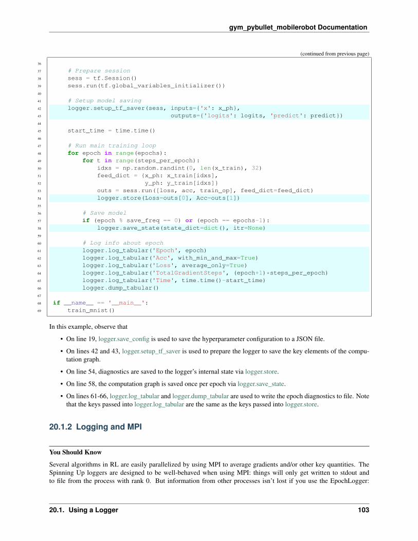
gym_pybullet_mobilerobot Documentation

(continued from previous page)

36

37 # Prepare session38 sess = tf.Session()39 sess.run(tf.global_variables_initializer())40

41 # Setup model saving42 logger.setup_tf_saver(sess, inputs={'x': x_ph},43 outputs={'logits': logits, 'predict': predict})44

45 start_time = time.time()46

47 # Run main training loop48 for epoch in range(epochs):49 for t in range(steps_per_epoch):50 idxs = np.random.randint(0, len(x_train), 32)51 feed_dict = {x_ph: x_train[idxs],52 y_ph: y_train[idxs]}53 outs = sess.run([loss, acc, train_op], feed_dict=feed_dict)54 logger.store(Loss=outs[0], Acc=outs[1])55

56 # Save model57 if (epoch % save_freq == 0) or (epoch == epochs-1):58 logger.save_state(state_dict=dict(), itr=None)59

60 # Log info about epoch61 logger.log_tabular('Epoch', epoch)62 logger.log_tabular('Acc', with_min_and_max=True)63 logger.log_tabular('Loss', average_only=True)64 logger.log_tabular('TotalGradientSteps', (epoch+1)*steps_per_epoch)65 logger.log_tabular('Time', time.time()-start_time)66 logger.dump_tabular()67

68 if __name__ == '__main__':69 train_mnist()

In this example, observe that

• On line 19, logger.save_config is used to save the hyperparameter configuration to a JSON file.

• On lines 42 and 43, logger.setup_tf_saver is used to prepare the logger to save the key elements of the compu-tation graph.

• On line 54, diagnostics are saved to the logger’s internal state via logger.store.

• On line 58, the computation graph is saved once per epoch via logger.save_state.

• On lines 61-66, logger.log_tabular and logger.dump_tabular are used to write the epoch diagnostics to file. Notethat the keys passed into logger.log_tabular are the same as the keys passed into logger.store.

20.1.2 Logging and MPI

You Should Know

Several algorithms in RL are easily parallelized by using MPI to average gradients and/or other key quantities. TheSpinning Up loggers are designed to be well-behaved when using MPI: things will only get written to stdout andto file from the process with rank 0. But information from other processes isn’t lost if you use the EpochLogger:

20.1. Using a Logger 103

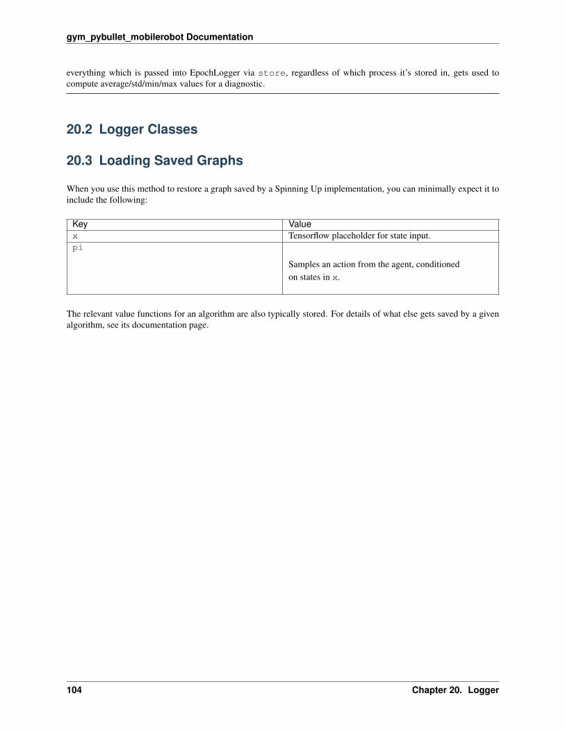
gym_pybullet_mobilerobot Documentation

everything which is passed into EpochLogger via store, regardless of which process it’s stored in, gets used tocompute average/std/min/max values for a diagnostic.

20.2 Logger Classes

20.3 Loading Saved Graphs

When you use this method to restore a graph saved by a Spinning Up implementation, you can minimally expect it toinclude the following:

Key Valuex Tensorflow placeholder for state input.pi

Samples an action from the agent, conditionedon states in x.

The relevant value functions for an algorithm are also typically stored. For details of what else gets saved by a givenalgorithm, see its documentation page.

104 Chapter 20. Logger

CHAPTER 21

Plotter

See the page on plotting results for documentation of the plotter.

105

gym_pybullet_mobilerobot Documentation

106 Chapter 21. Plotter

CHAPTER 22

MPI Tools

Table of Contents

• MPI Tools

– Core MPI Utilities

– MPI + Tensorflow Utilities

22.1 Core MPI Utilities

22.2 MPI + Tensorflow Utilities

The spinup.utils.mpi_tf contains a a few tools to make it easy to use the AdamOptimizer across many MPIprocesses. This is a bit hacky—if you’re looking for something more sophisticated and general-purpose, considerhorovod.

107

gym_pybullet_mobilerobot Documentation

108 Chapter 22. MPI Tools

CHAPTER 23

Run Utils

Table of Contents

• Run Utils

– ExperimentGrid

– Calling Experiments

23.1 ExperimentGrid

Spinning Up ships with a tool called ExperimentGrid for making hyperparameter ablations easier. This is based on(but simpler than) the rllab tool called VariantGenerator.

23.2 Calling Experiments

109

gym_pybullet_mobilerobot Documentation

110 Chapter 23. Run Utils

CHAPTER 24

Indices and tables

• genindex

• modindex

• search

111

gym_pybullet_mobilerobot Documentation

112 Chapter 24. Indices and tables

Index

Symbols-act, -ac_kwargs:activation

command line option, 18-count

command line option, 28-cpu, -num_cpu

command line option, 18-data_dir

command line option, 18-datestamp

command line option, 18-env, -env_name

command line option, 17-exclude=[EXC ...]

command line option, 28-exp_name

command line option, 18-hid, -ac_kwargs:hidden_sizes

command line option, 18-select=[SEL ...]

command line option, 28-d, -deterministic

command line option, 24-i I, -itr=I, default=-1

command line option, 24-l L, -len=L, default=0

command line option, 24-l, -legend=[LEGEND ...]

command line option, 27-n N, -episodes=N, default=100

command line option, 24-nr, -norender

command line option, 24-s, -smooth=S, default=1

command line option, 28-x, -xaxis=XAXIS,

default=’TotalEnvInteracts’command line option, 28

-y, -value=[VALUE ...],

default=’Performance’command line option, 28

Ccommand line option

-act, -ac_kwargs:activation, 18-count, 28-cpu, -num_cpu, 18-data_dir, 18-datestamp, 18-env, -env_name, 17-exclude=[EXC ...], 28-exp_name, 18-hid, -ac_kwargs:hidden_sizes, 18-select=[SEL ...], 28-d, -deterministic, 24-i I, -itr=I, default=-1, 24-l L, -len=L, default=0, 24-l, -legend=[LEGEND ...], 27-n N, -episodes=N, default=100, 24-nr, -norender, 24-s, -smooth=S, default=1, 28-x, -xaxis=XAXIS,

default=’TotalEnvInteracts’,28

-y, -value=[VALUE ...],default=’Performance’, 28

logdir, 27

Llogdir

command line option, 27

113