Group MeetingGroup Meeting

2010/03/16 R98229014 Kirsten Feng2010/03/16 R98229014 Kirsten Feng

Coupled Decadal Variability Coupled Decadal Variability in the North Pacific: An in the North Pacific: An

Observationally Observationally ConstrainedConstrained

Idealized Model*Idealized Model*

BO QIU, NIKLAS SCHNEIDER, BO QIU, NIKLAS SCHNEIDER, AND SHUIMING CHENAND SHUIMING CHEN

Goal Goal

Decadal-to-multidecadal time-scale SST vDecadal-to-multidecadal time-scale SST variability in a midlatitude ocean can be genariability in a midlatitude ocean can be generated through three different scenarios.erated through three different scenarios.1. climate noise scenario1. climate noise scenario2. ocean circulation and its slow response in c2. ocean circulation and its slow response in c

ontributing to the reddening of the SST signalontributing to the reddening of the SST signals (improve the predictive skill)s (improve the predictive skill)

3. ocean dynamics 3. ocean dynamics and and its feedback to the atits feedback to the atmospheric circulationmospheric circulation

Goal Goal

To explore the relevance of the above To explore the relevance of the above three scenarios by analysis of available three scenarios by analysis of available observational data and adoption of observational data and adoption of idealized models with different dynamic idealized models with different dynamic complexities.complexities.

To realize the mode in which ocean To realize the mode in which ocean circulation changes are expected to play circulation changes are expected to play an active role.an active role.

Experiment Experiment

I. NO SST feedback:I. NO SST feedback: In the absence of the SST feedback, the In the absence of the SST feedback, the

intrinsic atmospheric forcing enhances the intrinsic atmospheric forcing enhances the decadal and longer time-scale SST variance decadal and longer time-scale SST variance through oceanic advection but fails to capture through oceanic advection but fails to capture the observed decadal spectral peak.the observed decadal spectral peak.

Experiment Experiment

II. SST feedback:II. SST feedback:

KE SSTKE SST Wind stress curlWind stress curl

SSHaSSHaShift KE jetShift KE jet

Ekman DivergenceEkman Divergence

++

-- Alter the sign of SSAlter the sign of SSTaTa

Experiment Experiment

Climate noise model for SST with the adveClimate noise model for SST with the advective effectctive effecta. Oceanic adjustment to the changing wind sta. Oceanic adjustment to the changing wind st

ress fieldress fieldb. SSH-induced SST changes in the KE bandb. SSH-induced SST changes in the KE band

Experiment Experiment

Coupled versus uncoupled variabilityCoupled versus uncoupled variabilitya. Air–sea uncoupled case (ba. Air–sea uncoupled case (b==0)0)b. Air–sea coupled case (bb. Air–sea coupled case (b≠≠0)0)c. Parameter sensitivityc. Parameter sensitivity

Why KEWhy KE

Commonly based on Commonly based on EOF analysis of winter EOF analysis of winter time SST signalstime SST signals

SSTa and PDO indexSSTa and PDO index

Observation and modelObservation and model

Conclusion Conclusion

Satellite altimeter measurements of the Satellite altimeter measurements of the past decade have shown that the low-past decade have shown that the low-frequency KE variability is dominated by frequency KE variability is dominated by concurrent changes in the strength and concurrent changes in the strength and path of the KE jet. A strengthened path of the KE jet. A strengthened (weakened) KE jet tends to be (weakened) KE jet tends to be accompanied by a northerly (southerly) accompanied by a northerly (southerly) path, giving rise to a positive (negative) path, giving rise to a positive (negative) regional SSH anomaly.regional SSH anomaly.

Forcing of Low-Frequency OceaForcing of Low-Frequency Ocean Variability in the Northeast Pacn Variability in the Northeast Pac

ific*ific*

KETTYAH C. CHHAK, EMANUELE DI KETTYAH C. CHHAK, EMANUELE DI LORENZO, NIKLAS SCHNEIDER, ANLORENZO, NIKLAS SCHNEIDER, AN

D PATRICK F. CUMMINSD PATRICK F. CUMMINS

EOF of SSTa EOF of SSTa

1st mode: PDO1st mode: PDOSST, SSHSST, SSHALAL↔PDO↔PDOMonopole structureMonopole structure

2nd mode: NPGO2nd mode: NPGOSSS (sea surface salinities)SSS (sea surface salinities)NPGONPGO→NPO→NPODipole structureDipole structure

Goal Goal

To examine and compare the forcing To examine and compare the forcing mechanisms and underlying ocean dynamics of mechanisms and underlying ocean dynamics of two dominant modes of ocean variability in the two dominant modes of ocean variability in the northeast Pacific (NEP).northeast Pacific (NEP).

To study how the atmospheric forcing drives the To study how the atmospheric forcing drives the SST and SSH anomalies.SST and SSH anomalies.

In this paper, we show how the NPGO together In this paper, we show how the NPGO together with the PDO contributes to a more complete with the PDO contributes to a more complete characterization of NEP climate variability.characterization of NEP climate variability.

Model Model

The ocean model experiments in this study The ocean model experiments in this study were conducted with the Regional Ocean Mwere conducted with the Regional Ocean Modeling System (ROMS), a odeling System (ROMS), a free-surfacefree-surface, , hhydrostaticydrostatic, , primitive-equationprimitive-equation ocean mod ocean model with el with terrain-following coordinatesterrain-following coordinates in th in the vertical and generalized e vertical and generalized orthogonal curvorthogonal curvilinear coordinatesilinear coordinates in the horizontal. in the horizontal.

Model Model

split-explicit time-stepping schemesplit-explicit time-stepping schemespecial coupling between barotropic (fast) special coupling between barotropic (fast)

and baroclinic (slow) modesand baroclinic (slow) modes three open boundariesthree open boundariessurface forcing monthly mean wind stress fsurface forcing monthly mean wind stress f

rom NCEProm NCEPdomain covering 25–61N, 179–111Wdomain covering 25–61N, 179–111W

encompassing: the Gulf of Alaska (GOA), the California Current encompassing: the Gulf of Alaska (GOA), the California Current System (CCS), and portions of the North Pacific subpolar and suSystem (CCS), and portions of the North Pacific subpolar and subtropical gyres.)btropical gyres.)

Modes of decadal variabilityModes of decadal variability

Properties of the PDO and NPGOProperties of the PDO and NPGOComparison with satellite observationsComparison with satellite observationsAtmospheric forcing of the PDO and NPGAtmospheric forcing of the PDO and NPG

OO

Properties of the PDO and NPGOProperties of the PDO and NPGO FIG. 1. (a) Time series of the observed PDO index FIG. 1. (a) Time series of the observed PDO index

(gray line) and PC1 of SSHA (i.e., the model PDO in(gray line) and PC1 of SSHA (i.e., the model PDO index) (black line), PC1 of SSTA (red line), and PC2 of dex) (black line), PC1 of SSTA (red line), and PC2 of SSSA (blue line) of the ocean model hindcast. All tiSSSA (blue line) of the ocean model hindcast. All time series are plotted in standard deviation units witme series are plotted in standard deviation units with the 2-yr low-passed time series plotted in bold. (b) h the 2-yr low-passed time series plotted in bold. (b) Time series of PC2 of SSHA (i.e., the model NPGO iTime series of PC2 of SSHA (i.e., the model NPGO index; black line), PC2 of SSTA (red line), and PC1 ondex; black line), PC2 of SSTA (red line), and PC1 of SSSA (blue line). Regression maps of the model f SSSA (blue line). Regression maps of the model (c) PDO and (d) NPGO index, respectively, with the (c) PDO and (d) NPGO index, respectively, with the model SSHA. White (black) contours correspond to rmodel SSHA. White (black) contours correspond to regions of positive (negative) Ekman pumping and aregions of positive (negative) Ekman pumping and are based on a regression of the model PDO and NPe based on a regression of the model PDO and NPGO index with the NCEP wind stress curl. (e)–(h) BlGO index with the NCEP wind stress curl. (e)–(h) Black arrows correspond to wind-driven Ekman currenack arrows correspond to wind-driven Ekman currents based on a regression of the model PDO and NPts based on a regression of the model PDO and NPGO index with the model ocean currents. RegressioGO index with the model ocean currents. Regression maps of the model (e) PDO and (f) NPGO index wn maps of the model (e) PDO and (f) NPGO index with the model SSTA. White contours correspond to tith the model SSTA. White contours correspond to the climatological mean SST gradients with cooler She climatological mean SST gradients with cooler SSTs in the GOA. Regression maps of the model (g) STs in the GOA. Regression maps of the model (g) PDO and (h) NPGO index with the model SSSA. WhPDO and (h) NPGO index with the model SSSA. White contours correspond to the climatological mean Site contours correspond to the climatological mean SSS gradients with fresher waters in the GOA. The pSS gradients with fresher waters in the GOA. The percentage explained variance by each regression mercentage explained variance by each regression map is denoted in (a)–(h).ap is denoted in (a)–(h).

Comparison with satellite observatiComparison with satellite observationsons

FIG. 2. The difference betweeFIG. 2. The difference between PDO and NPGO regression n PDO and NPGO regression maps of (a) SSHA, (b) SST, amaps of (a) SSHA, (b) SST, and (c) SSS. White contour linnd (c) SSS. White contour lines denote where the PDO does denote where the PDO dominates while black contour liminates while black contour lines denote where the NPGO nes denote where the NPGO dominates.dominates.

Comparison with satellite observatiComparison with satellite observationsons

Atmospheric forcing of the PDO anAtmospheric forcing of the PDO and NPGOd NPGO

FIG. 4. Regression maps of the model (a) FIG. 4. Regression maps of the model (a) PDO index and (c) NPGO index with North PDO index and (c) NPGO index with North Pacific NCEP SLPA illustrating the spatial Pacific NCEP SLPA illustrating the spatial patterns of atmospheric forcing associated patterns of atmospheric forcing associated with each mode. Black arrows correspond with each mode. Black arrows correspond to wind stress vectors based on a regressito wind stress vectors based on a regression of the model PDO and NPGO index witon of the model PDO and NPGO index with NCEP wind stress. Also shown are the tih NCEP wind stress. Also shown are the time series of the model (b) PDO and (d) Nme series of the model (b) PDO and (d) NPGOindex in black and (b) PDO and (d) NPGOindex in black and (b) PDO and (d) NPGO index reconstructions from an AR-1 pPGO index reconstructions from an AR-1 process forced by some prescribed forcing f rocess forced by some prescribed forcing f t . The red lines are reconstructions from f t . The red lines are reconstructions from f t that are defined as the SLPA averaged ovt that are defined as the SLPA averaged over the NEP [red box in (a) for the PDO and er the NEP [red box in (a) for the PDO and the difference between the SLPA averaged the difference between the SLPA averaged over the top red box in (b) and the SLPA aover the top red box in (b) and the SLPA averaged over the bottom red box in (b) for tveraged over the bottom red box in (b) for the NPGO. The green lines are reconstructihe NPGO. The green lines are reconstructions from f t that is defined as PC1 (NP indons from f t that is defined as PC1 (NP index) and PC2 (NPO index) of North Pacific ex) and PC2 (NPO index) of North Pacific SLP.SLP.

Budget analysis -- SSTBudget analysis -- SST FIG. 5. The regression map of the model FIG. 5. The regression map of the model

PDO index with the (a) model SSTA and PDO index with the (a) model SSTA and (b) sum of the SST budget terms. The pa(b) sum of the SST budget terms. The pattern correlation between the anomalies fttern correlation between the anomalies from reconstructed budget and the regresrom reconstructed budget and the regression map is 0.76 (.99% significant). The sion map is 0.76 (.99% significant). The SST budget terms for the PDO, including SST budget terms for the PDO, including (c) anomalous horizontal advection of me(c) anomalous horizontal advection of mean SST gradients, (d) anomalous vertical an SST gradients, (d) anomalous vertical temperature advection via wind driven Ektemperature advection via wind driven Ekman pumping, (e) mean horizontal advecman pumping, (e) mean horizontal advection of anomalous SST gradients, (f) meation of anomalous SST gradients, (f) mean vertical advection of temperature anomn vertical advection of temperature anomalies via Ekman pumping, and (g) heatinalies via Ekman pumping, and (g) heating from anomalous net surface heat fluxeg from anomalous net surface heat fluxes. The white contours in (c) and (e) are ths. The white contours in (c) and (e) are the mean and anomalous SST gradients, re mean and anomalous SST gradients, respectively, while the black arrows in (c) espectively, while the black arrows in (c) and (e) are the mean and anomalous surand (e) are the mean and anomalous surface currents, respectively.face currents, respectively.

Budget analysis -- SSTBudget analysis -- SST

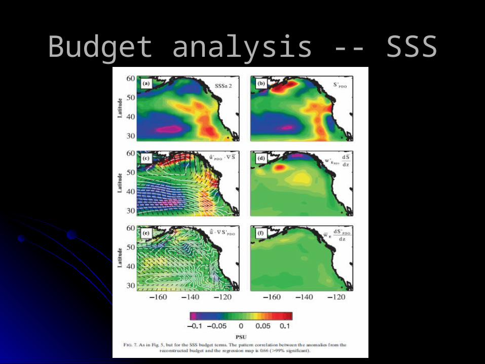
Budget analysis -- SSSBudget analysis -- SSS

Budget analysis -- SSSBudget analysis -- SSS

Budget analysis -- SSSBudget analysis -- SSS

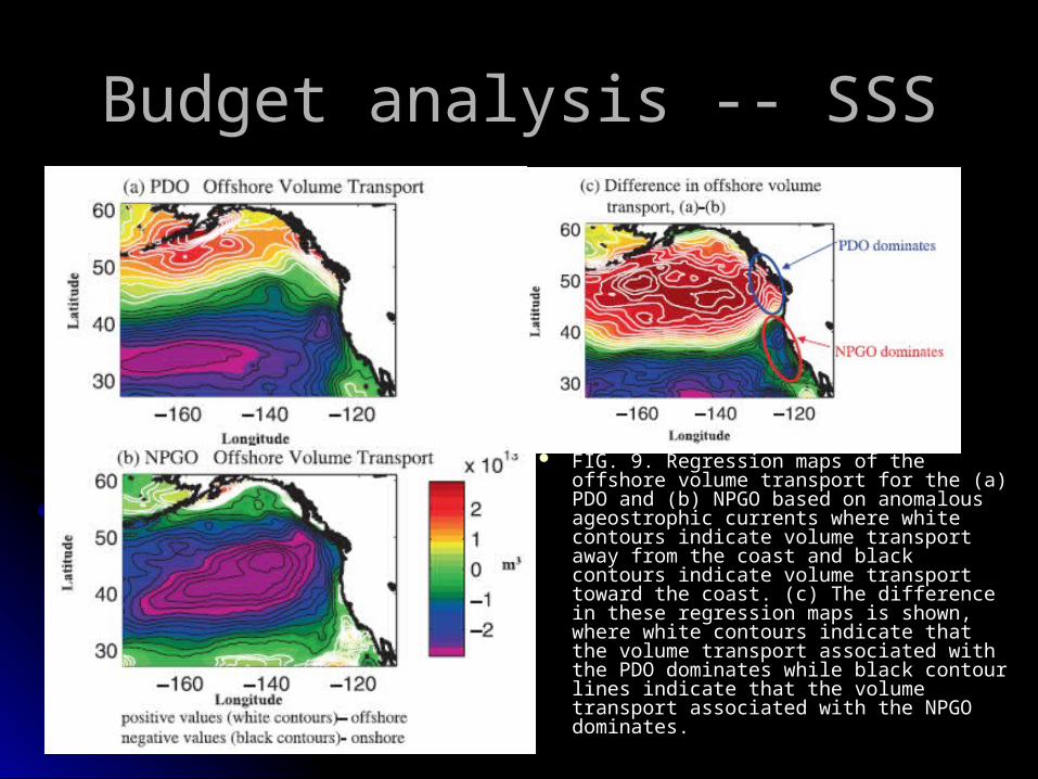
FIG. 9. Regression maps of the offshore FIG. 9. Regression maps of the offshore volume transport for thevolume transport for the (a) PDO and (b) (a) PDO and (b) NPGO based on anomalous ageostrophic NPGO based on anomalous ageostrophic currentscurrents where white contours indicate where white contours indicate volume transport away fromvolume transport away from the coast and the coast and black contours indicate volume transport black contours indicate volume transport toward thetoward the coast. (c) The difference in coast. (c) The difference in these regression maps is shown, wherethese regression maps is shown, where white contours indicate that the volume white contours indicate that the volume transport associated withtransport associated with the PDO the PDO dominates while black contour lines dominates while black contour lines indicate that theindicate that the volume transport volume transport associated with the NPGO dominates.associated with the NPGO dominates.

Shaping of the PDO and NPGO Shaping of the PDO and NPGO modesmodes

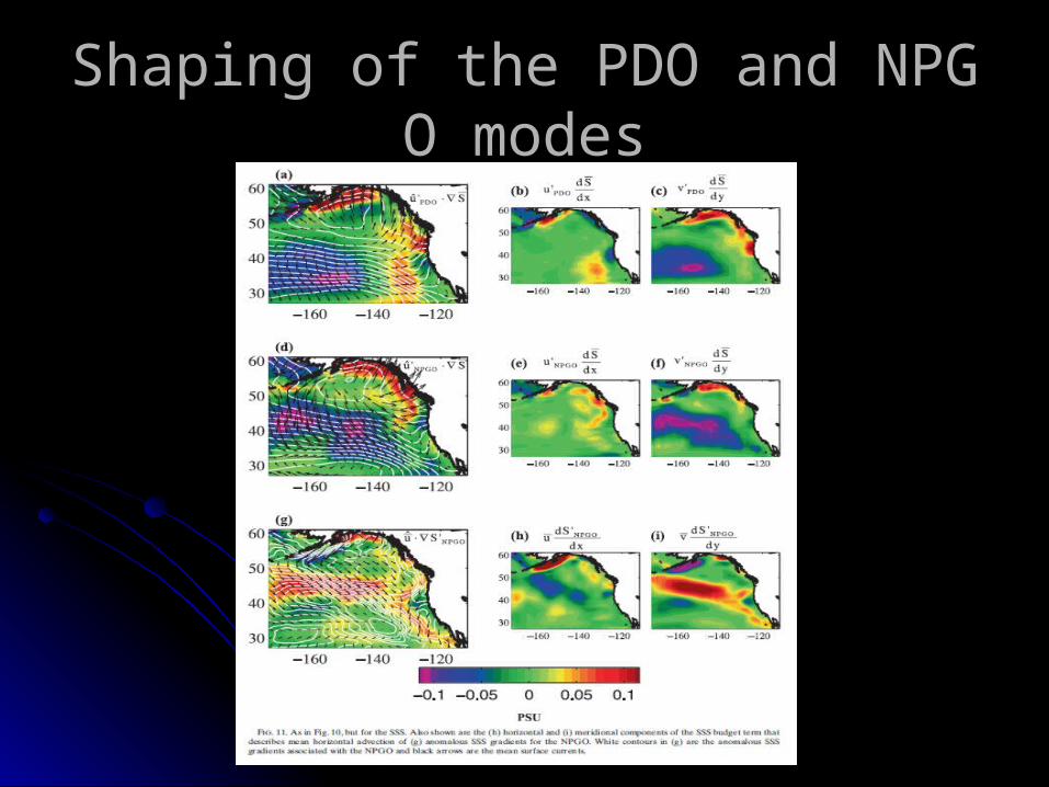
Shaping of the PDO and NPGO moShaping of the PDO and NPGO modesdes

Vertical expression of PDO and NPVertical expression of PDO and NPGO modesGO modes

Conclusion Conclusion

The shallowness of the modes, the depth The shallowness of the modes, the depth of the mean mixed layer, and wintertime of the mean mixed layer, and wintertime temperature profile inversions contribute to temperature profile inversions contribute to the sensitivity of the budget analysis in the the sensitivity of the budget analysis in the regions of reduced reconstruction skill.regions of reduced reconstruction skill.

Conclusion Conclusion

Results show that the basinwide SST and SSS aResults show that the basinwide SST and SSS anomaly patterns associated with each mode are nomaly patterns associated with each mode are shaped primarily by anomalous horizontal advecshaped primarily by anomalous horizontal advection of mean surface temperature and salinity grtion of mean surface temperature and salinity gradients (adients (▽▽T and T and ▽▽ S) via anomalous surface E S) via anomalous surface Ekman currents.kman currents.

Vertical profiles of the PDO and NPGO indicate tVertical profiles of the PDO and NPGO indicate that the modes are strongest mainly in the upper hat the modes are strongest mainly in the upper ocean down to 250 m.ocean down to 250 m.

Thank youThank you～～♪ ♪ ♪♪