idealized test cases for the dynamical cores of ...cjablono/ncar_asp_2008_idealized_testcases... ·...
TRANSCRIPT
Idealized test cases for the dynamical cores ofAtmospheric General Circulation Models:
A proposal for the NCAR ASP 2008 summer colloquium
Christiane Jablonowski (University of Michgan)Peter Lauritzen (NCAR)
Ram Nair (NCAR)Mark Taylor (Sandia National Laboratory)
May/29/2008
1 Idealized test cases for 3D dynamical coresThis document describes the idealized dynamical core test cases that are proposed for the NCARASP Summer Colloquium in June 2008. All test cases are dry and adiabatic. No physical pa-rameterizations or vertical diffusion are applied. All dynamical cores should be run in theiroperational configurations which includes the typical diffusion mechanisms and coefficients,filters, time steps and other tunable parameters. In addition, the runs should utilizes their stan-dard a posteriori fixers like mass or energy fixers if applicable. These standard runs serve ascontrol simulations. All parameters and fixers need to be documented to foster model compar-isons. In addition, the documentation needs to list the prognostic variables, the equation set(e.g. shallow-atmosphere hydrostatic, or shallow-atmosphere nonhydrostatic), the horizontalgrid staggering, time stepping approach, vertical coordinate, and horizontal and vertical resolu-tions.
The modeling groups are also invited to test their models in non-operational configurationsthat, for example, use less explicit diffusion. In particular, Rayleigh friction at the model topshould be avoided if applied. These non-standard configurations are often viable for idealizedtest cases as considered here, but note that they might not be applicable in real weather orclimate simulations. Therefore, any conclusions need to be carefully drawn and are not neces-sarily valid for models with physics parameterizations. More details are provided in section 2.The parameter p0 in models with hybrid η coordinates in the vertical direction needs be set top0 = 1000 hPa which might not be the standard choice.
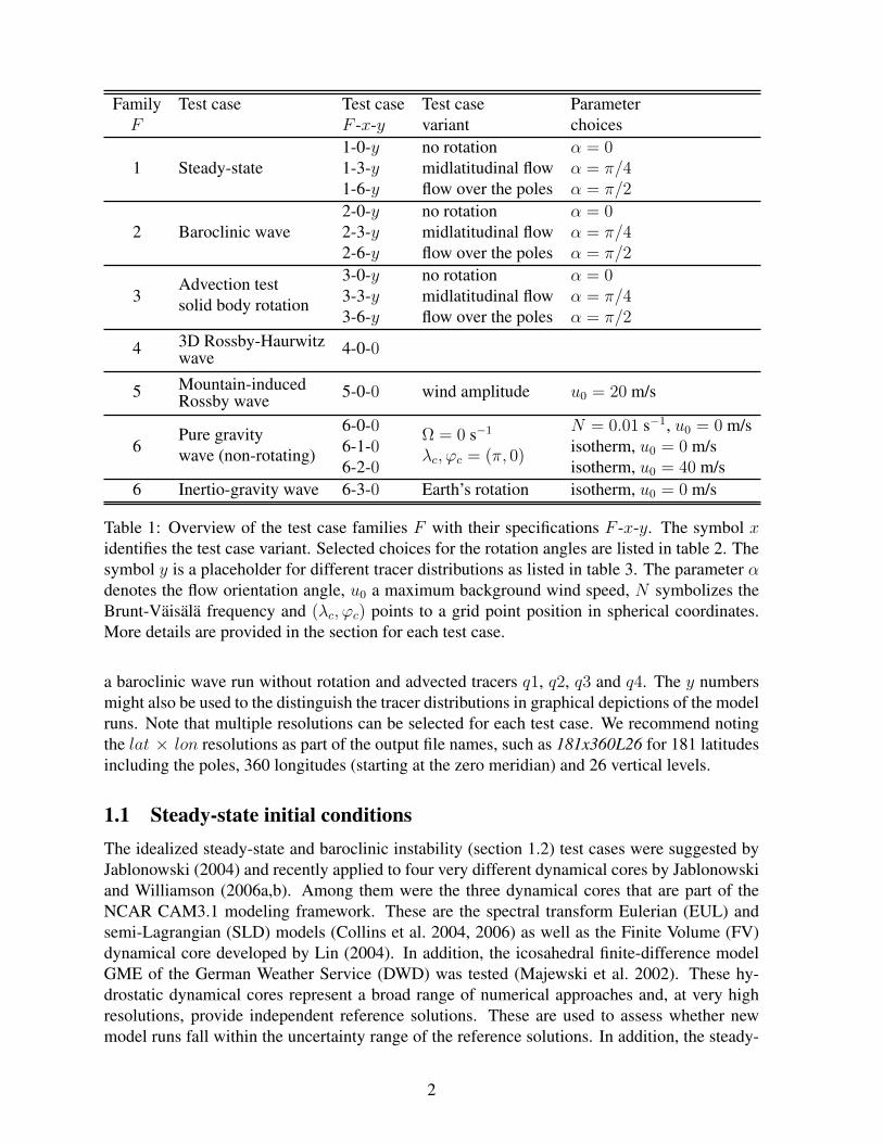
Table 1 lists all test case that are proposed for the NCAR ASP summer program. We suggestusing the unique multiple-digit test case number F − x − y from column 3 to distinguish themodel runs. The first digit identifies the test case family F . The second digit x indicates avariation of the initial conditions such as a different rotation angle or background velocity. Thex choices for selected rotation angles are listed in Table 2. The optional third digit y denotesa specific tracer distribution if applicable. An overview of the tracer distributions y is givenin table 3. It is encouraged to transport all tracers during a single model run. Then the tracernumbers y can be concatenated to form a longer identifier, such as 2-0-1234 which denotes
1
Family Test case Test case Test case ParameterF F -x-y variant choices
1-0-y no rotation α = 01 Steady-state 1-3-y midlatitudinal flow α = π/4
1-6-y flow over the poles α = π/2
2-0-y no rotation α = 02 Baroclinic wave 2-3-y midlatitudinal flow α = π/4
2-6-y flow over the poles α = π/2
3-0-y no rotation α = 03
Advection test3-3-y midlatitudinal flow α = π/4solid body rotation3-6-y flow over the poles α = π/2
3D Rossby-Haurwitz4 wave 4-0-0
Mountain-induced5 Rossby wave 5-0-0 wind amplitude u0 = 20 m/s
6-0-0 N = 0.01 s−1, u0 = 0 m/s6
Pure gravity6-1-0
Ω = 0 s−1
isotherm, u0 = 0 m/swave (non-rotating)6-2-0
λc, ϕc = (π, 0)isotherm, u0 = 40 m/s
6 Inertio-gravity wave 6-3-0 Earth’s rotation isotherm, u0 = 0 m/s
Table 1: Overview of the test case families F with their specifications F -x-y. The symbol xidentifies the test case variant. Selected choices for the rotation angles are listed in table 2. Thesymbol y is a placeholder for different tracer distributions as listed in table 3. The parameter αdenotes the flow orientation angle, u0 a maximum background wind speed, N symbolizes theBrunt-Vaisala frequency and (λc, ϕc) points to a grid point position in spherical coordinates.More details are provided in the section for each test case.
a baroclinic wave run without rotation and advected tracers q1, q2, q3 and q4. The y numbersmight also be used to the distinguish the tracer distributions in graphical depictions of the modelruns. Note that multiple resolutions can be selected for each test case. We recommend notingthe lat × lon resolutions as part of the output file names, such as 181x360L26 for 181 latitudesincluding the poles, 360 longitudes (starting at the zero meridian) and 26 vertical levels.
1.1 Steady-state initial conditionsThe idealized steady-state and baroclinic instability (section 1.2) test cases were suggested byJablonowski (2004) and recently applied to four very different dynamical cores by Jablonowskiand Williamson (2006a,b). Among them were the three dynamical cores that are part of theNCAR CAM3.1 modeling framework. These are the spectral transform Eulerian (EUL) andsemi-Lagrangian (SLD) models (Collins et al. 2004, 2006) as well as the Finite Volume (FV)dynamical core developed by Lin (2004). In addition, the icosahedral finite-difference modelGME of the German Weather Service (DWD) was tested (Majewski et al. 2002). These hy-drostatic dynamical cores represent a broad range of numerical approaches and, at very highresolutions, provide independent reference solutions. These are used to assess whether newmodel runs fall within the uncertainty range of the reference solutions. In addition, the steady-
2
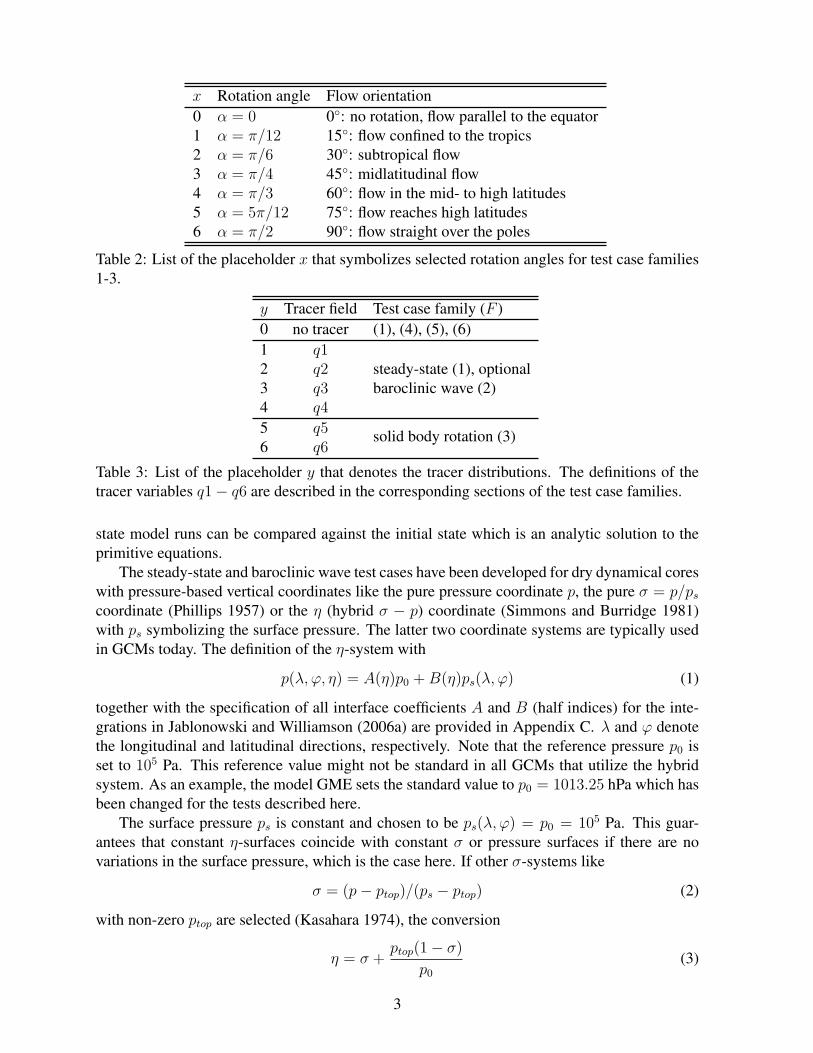
x Rotation angle Flow orientation0 α = 0 0: no rotation, flow parallel to the equator1 α = π/12 15: flow confined to the tropics2 α = π/6 30: subtropical flow3 α = π/4 45: midlatitudinal flow4 α = π/3 60: flow in the mid- to high latitudes5 α = 5π/12 75: flow reaches high latitudes6 α = π/2 90: flow straight over the poles
Table 2: List of the placeholder x that symbolizes selected rotation angles for test case families1-3.
y Tracer field Test case family (F )0 no tracer (1), (4), (5), (6)1 q12 q2 steady-state (1), optional3 q3 baroclinic wave (2)4 q4
5 q56 q6
solid body rotation (3)
Table 3: List of the placeholder y that denotes the tracer distributions. The definitions of thetracer variables q1− q6 are described in the corresponding sections of the test case families.
state model runs can be compared against the initial state which is an analytic solution to theprimitive equations.
The steady-state and baroclinic wave test cases have been developed for dry dynamical coreswith pressure-based vertical coordinates like the pure pressure coordinate p, the pure σ = p/ps
coordinate (Phillips 1957) or the η (hybrid σ − p) coordinate (Simmons and Burridge 1981)with ps symbolizing the surface pressure. The latter two coordinate systems are typically usedin GCMs today. The definition of the η-system with
p(λ, ϕ, η) = A(η)p0 +B(η)ps(λ, ϕ) (1)
together with the specification of all interface coefficients A and B (half indices) for the inte-grations in Jablonowski and Williamson (2006a) are provided in Appendix C. λ and ϕ denotethe longitudinal and latitudinal directions, respectively. Note that the reference pressure p0 isset to 105 Pa. This reference value might not be standard in all GCMs that utilize the hybridsystem. As an example, the model GME sets the standard value to p0 = 1013.25 hPa which hasbeen changed for the tests described here.
The surface pressure ps is constant and chosen to be ps(λ, ϕ) = p0 = 105 Pa. This guar-antees that constant η-surfaces coincide with constant σ or pressure surfaces if there are novariations in the surface pressure, which is the case here. If other σ-systems like
σ = (p− ptop)/(ps − ptop) (2)
with non-zero ptop are selected (Kasahara 1974), the conversion
η = σ +ptop(1− σ)
p0
(3)
3
can be used in the equations below. This expression recovers η = σ for ptop = 0 hPa. In general,the choice of the vertical coordinate system is left to the modeling group despite the fact thateach vertical coordinate system implies a different boundary condition for the vertical velocity.In practice, this has been found to be insignificant for the steady state test or the evolution ofthe baroclinic wave over a 10-day time period. If other generalized vertical coordinate systemsare used, like height-based or hybrid isentropic-σ levels, either an iterative method or verticalinterpolations of the initial conditions become necessary. Details of the iterative method, whichis the preferred choice, are provided in Appendix D
The initial state is defined by analytic expressions in spherical (λ, ϕ, η) coordinates whereλ ∈ [0, 2π] stands for the longitude, ϕ ∈ [−π/2, π/2] represents the latitude and η ∈ [0, 1]denotes the position in the vertical direction which is unity at the surface and approaches zeroat the model top. The subsequent expressions can also be straightforwardly transformed intodifferent, e.g. Cartesian, coordinate systems. All physical constants used in the test specificationare listed below and in Appendix G. Users of the test case are encouraged to select the sameparameter set in their models to foster model intercomparisons.
Assuming that a model utilizes η-levels an auxiliary variable ηv is defined by
ηv = (η − η0)π
2(4)
with η0 = 0.252. Eq. (4) can also be directly applied to models with pure pressure coordinatesif η = p/ps is adopted at each pressure level p (for models with ptop = 0 hPa)..
The flow field is comprised of two symmetric zonal jets in midlatitudes. The zonal wind uand meridional wind v are defined as
u(λ, ϕ, η) = u0 cos32 ηv sin2 (2ϕ) (5)
v(λ, ϕ, η) = 0 m s−1. (6)
Here the maximum amplitude u0 is set to 35 m s−1 which is close to the wind speed of thezonal-mean time-mean jet streams in the troposphere. In addition, the vertical velocity is set tozero for non-hydrostatic setups. This flow field in nondivergent and allows the derivation of theanalytic initial data even for models in vorticity-divergence (ζ ,δ) form. In particular, the radialoutward component of the relative vorticity ζ is given by
ζ(λ, ϕ, η) =− 4 u0
acos
32 ηv sinϕ cosϕ (2− 5 sin2 ϕ) (7)
and δ = 0 s−1 is automatically fulfilled. a = 6.371229× 10⁶ m indicates the mean radius of theEarth.
The horizontally averaged temperature T (η) is split into two representations for the lower(Eq. (8)) and middle (Eq. (9)) atmosphere. This introduces the characteristic atmospheric tem-perature profiles especially at upper levels. They are given by
T (η) = T0 ηRdΓ
g (for ηs ≥ η ≥ ηt) (8)
T (η) = T0 ηRdΓ
g + ∆T (ηt − η)5 (for ηtop > η) (9)
with the surface level ηs = 1, the tropopause level ηt = 0.2 and the horizontal-mean temperatureat the surface T0 = 288 K. The temperature lapse rate Γ is set to 0.005 K m−1 which is similar
4
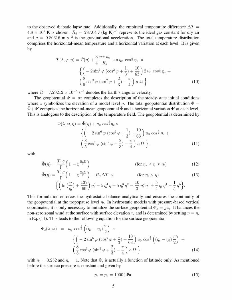
to the observed diabatic lapse rate. Additionally, the empirical temperature difference ∆T =4.8 × 10⁵ K is chosen. Rd = 287.04 J (kg K)−1 represents the ideal gas constant for dry airand g = 9.80616 m s−2 is the gravitational acceleration. The total temperature distributioncomprises the horizontal-mean temperature and a horizontal variation at each level. It is givenby
T (λ, ϕ, η) = T (η) +3
4
η π u0
Rd
sin ηv cos12 ηv ×
(− 2 sin6 ϕ (cos2 ϕ+
1
3) +
10
63
)2u0 cos
32 ηv +
( 8
5cos3 ϕ (sin2 ϕ+
2
3)− π
4
)a Ω
(10)
where Ω = 7.29212× 10⁻⁵ s−1 denotes the Earth’s angular velocity.The geopotential Φ = gz completes the description of the steady-state initial conditions
where z symbolizes the elevation of a model level η. The total geopotential distribution Φ =Φ+Φ′ comprises the horizontal-mean geopotential Φ and a horizontal variation Φ′ at each level.This is analogous to the description of the temperature field. The geopotential is determined by
Φ(λ, ϕ, η) = Φ(η) + u0 cos32ηv ×(
− 2 sin6 ϕ (cos2 ϕ+1
3) +
10
63
)u0 cos
32 ηv +
( 8
5cos3 ϕ (sin2 ϕ+
2
3)− π
4
)a Ω
. (11)
with
Φ(η) =T0 g
Γ
(1 − η
Rd Γ
g
)(for ηs ≥ η ≥ ηt) (12)
Φ(η) =T0 g
Γ
(1 − η
Rd Γ
g
)−Rd ∆T × (for ηt > η) (13)
(ln
( ηηt
)+
137
60
)η5
t − 5 η4t η + 5 η3
t η2 − 10
3η2
t η3 +
5
4ηt η
4 − 1
5η5
.
This formulation enforces the hydrostatic balance analytically and ensures the continuity ofthe geopotential at the tropopause level ηt. In hydrostatic models with pressure-based verticalcoordinates, it is only necessary to initialize the surface geopotential Φs = gzs. It balances thenon-zero zonal wind at the surface with surface elevation zs and is determined by setting η = ηs
in Eq. (11). This leads to the following equation for the surface geopotential
Φs(λ, ϕ) = u0 cos32
((ηs − η0)
π
2
)×
(− 2 sin6 ϕ (cos2 ϕ+
1
3) +
10
63
)u0 cos
32
((ηs − η0)
π
2
)+
( 8
5cos3 ϕ (sin2 ϕ+
2
3)− π
4
)a Ω
(14)
with η0 = 0.252 and ηs = 1. Note that Φs is actually a function of latitude only. As mentionedbefore the surface pressure is constant and given by
ps = p0 = 1000 hPa. (15)
5
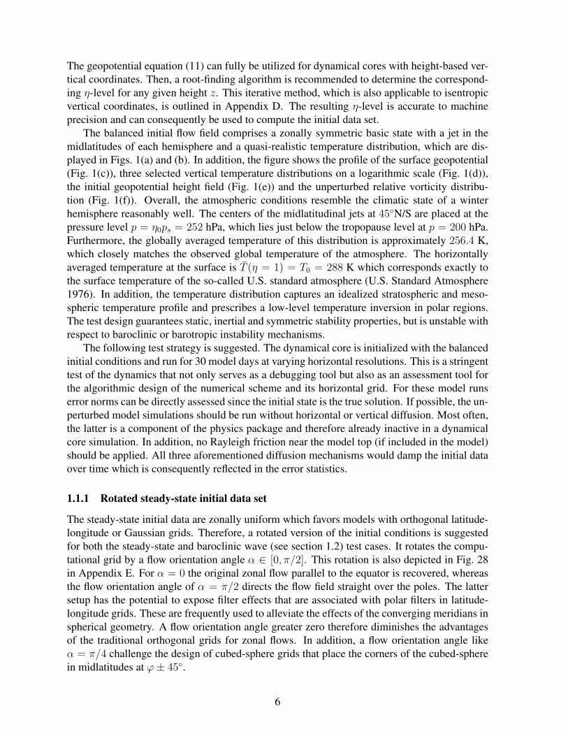
The geopotential equation (11) can fully be utilized for dynamical cores with height-based ver-tical coordinates. Then, a root-finding algorithm is recommended to determine the correspond-ing η-level for any given height z. This iterative method, which is also applicable to isentropicvertical coordinates, is outlined in Appendix D. The resulting η-level is accurate to machineprecision and can consequently be used to compute the initial data set.
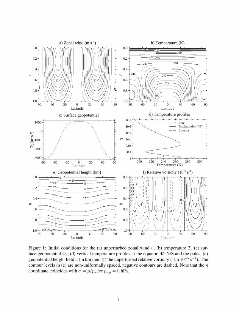
The balanced initial flow field comprises a zonally symmetric basic state with a jet in themidlatitudes of each hemisphere and a quasi-realistic temperature distribution, which are dis-played in Figs. 1(a) and (b). In addition, the figure shows the profile of the surface geopotential(Fig. 1(c)), three selected vertical temperature distributions on a logarithmic scale (Fig. 1(d)),the initial geopotential height field (Fig. 1(e)) and the unperturbed relative vorticity distribu-tion (Fig. 1(f)). Overall, the atmospheric conditions resemble the climatic state of a winterhemisphere reasonably well. The centers of the midlatitudinal jets at 45N/S are placed at thepressure level p = η0ps = 252 hPa, which lies just below the tropopause level at p = 200 hPa.Furthermore, the globally averaged temperature of this distribution is approximately 256.4 K,which closely matches the observed global temperature of the atmosphere. The horizontallyaveraged temperature at the surface is T (η = 1) = T0 = 288 K which corresponds exactly tothe surface temperature of the so-called U.S. standard atmosphere (U.S. Standard Atmosphere1976). In addition, the temperature distribution captures an idealized stratospheric and meso-spheric temperature profile and prescribes a low-level temperature inversion in polar regions.The test design guarantees static, inertial and symmetric stability properties, but is unstable withrespect to baroclinic or barotropic instability mechanisms.
The following test strategy is suggested. The dynamical core is initialized with the balancedinitial conditions and run for 30 model days at varying horizontal resolutions. This is a stringenttest of the dynamics that not only serves as a debugging tool but also as an assessment tool forthe algorithmic design of the numerical scheme and its horizontal grid. For these model runserror norms can be directly assessed since the initial state is the true solution. If possible, the un-perturbed model simulations should be run without horizontal or vertical diffusion. Most often,the latter is a component of the physics package and therefore already inactive in a dynamicalcore simulation. In addition, no Rayleigh friction near the model top (if included in the model)should be applied. All three aforementioned diffusion mechanisms would damp the initial dataover time which is consequently reflected in the error statistics.
1.1.1 Rotated steady-state initial data set
The steady-state initial data are zonally uniform which favors models with orthogonal latitude-longitude or Gaussian grids. Therefore, a rotated version of the initial conditions is suggestedfor both the steady-state and baroclinic wave (see section 1.2) test cases. It rotates the compu-tational grid by a flow orientation angle α ∈ [0, π/2]. This rotation is also depicted in Fig. 28in Appendix E. For α = 0 the original zonal flow parallel to the equator is recovered, whereasthe flow orientation angle of α = π/2 directs the flow field straight over the poles. The lattersetup has the potential to expose filter effects that are associated with polar filters in latitude-longitude grids. These are frequently used to alleviate the effects of the converging meridians inspherical geometry. A flow orientation angle greater zero therefore diminishes the advantagesof the traditional orthogonal grids for zonal flows. In addition, a flow orientation angle likeα = π/4 challenge the design of cubed-sphere grids that place the corners of the cubed-spherein midlatitudes at ϕ± 45.
6
0
9
9
9
9
9
9
18
18
18
18
27
27
27
27
a) Zonal wind (m s-1)0.0
0.2
0.4
0.6
0.8
1.0
η
-90 -60 -30 0 30 60 90Latitude
285
300
b) Temperature (K)0.0
0.2
0.4
0.6
0.8
1.0
η
-90 -60 -30 0 30 60 90Latitude
255
255
270
240
240240
240
240
225
225
210
c) Surface geopotential
-3000
-2000
-1000
0
1000
Φs (
m2
s-2)
-90 -60 -30 0 30 60 90Latitude
d) Temperature profiles1e-6
1e-51e-5
1e-4
1e-3
0.01
0.1
1
η
200 220 240 260 280 300Temperature (K)
EquatorMidlatitudes (45o)Pole
11
22
e) Geopotential height (km)0.0
0.2
0.4
0.6
0.8
1.0
η
-90 -60 -30 0 30 60 90Latitude
00
44
88
12121616
2040
-0.2-0.2
0 0 00.5
0.5
0.5
0.5
0.5
1
1
1.5-1.5
-1
-1
-0.5
-0.5
-0.5
-0.5
-0.5
0 0 0
f) Relative vorticity (10-5 s-1)0.0
0.2
0.4
0.6
0.8
1.0
η
-90 -60 -30 0 30 60 90Latitude
Figure 1: Initial conditions for the (a) unperturbed zonal wind u, (b) temperature T , (c) sur-face geopotential Φs, (d) vertical temperature profiles at the equator, 45N/S and the poles, (e)geopotential height field z (in km) and (f) the unperturbed relative vorticity ζ (in 10−5 s−1). Thecontour levels in (e) are non-uniformally spaced, negative contours are dashed. Note that the ηcoordinate coincides with σ = p/ps for ptop = 0 hPa.
7
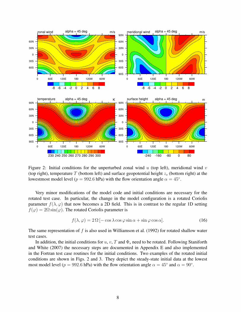
Figure 2: Initial conditions for the unperturbed zonal wind u (top left), meridional wind v(top right), temperature T (bottom left) and surface geopotential height zs (bottom right) at thelowestmost model level (p = 992.6 hPa) with the flow orientation angle α = 45.
Very minor modifications of the model code and initial conditions are necessary for therotated test case. In particular, the change in the model configuration is a rotated Coriolisparameter f(λ, ϕ) that now becomes a 2D field. This is in contrast to the regular 1D settingf(ϕ) = 2Ω sin(ϕ). The rotated Coriolis parameter is
f(λ, ϕ) = 2 Ω [− cosλ cosϕ sinα+ sinϕ cosα]. (16)
The same representation of f is also used in Williamson et al. (1992) for rotated shallow watertest cases.
In addition, the initial conditions for u, v, T and Φs need to be rotated. Following Staniforthand White (2007) the necessary steps are documented in Appendix E and also implementedin the Fortran test case routines for the initial conditions. Two examples of the rotated initialconditions are shown in Figs. 2 and 3. They depict the steady-state initial data at the lowestmost model level (p = 992.6 hPa) with the flow orientation angle α = 45 and α = 90.
8
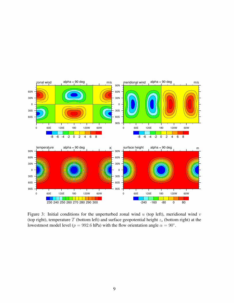
Figure 3: Initial conditions for the unperturbed zonal wind u (top left), meridional wind v(top right), temperature T (bottom left) and surface geopotential height zs (bottom right) at thelowestmost model level (p = 992.6 hPa) with the flow orientation angle α = 90.
9
1.1.2 Resolution, output data and analysis
We suggest running the steady-state test case with flow orientation angle α = 0 at the spectralresolutions T21, T42, T85 and T170 with 26 vertical levels. These resolutions correspondapproximately to the grid point resolutions 4 × 4, 2 × 2, 1 × 1 and 0.5 × 0.5. Similarinformation on the resolutions and time steps are provided in Appendix 2 that lists the choicesfor the three NCAR CAM3.5 dynamical cores and the icosahedral model GME.
We recommend repeating two rotated 30-day model run at the T85 spectral resolution or the1 × 1 grid point resolution with 26 vertical levels. The flow orientation angles are α = 45
and α = 90.For each model run the following instantaneous model variables to the NetCDF should be
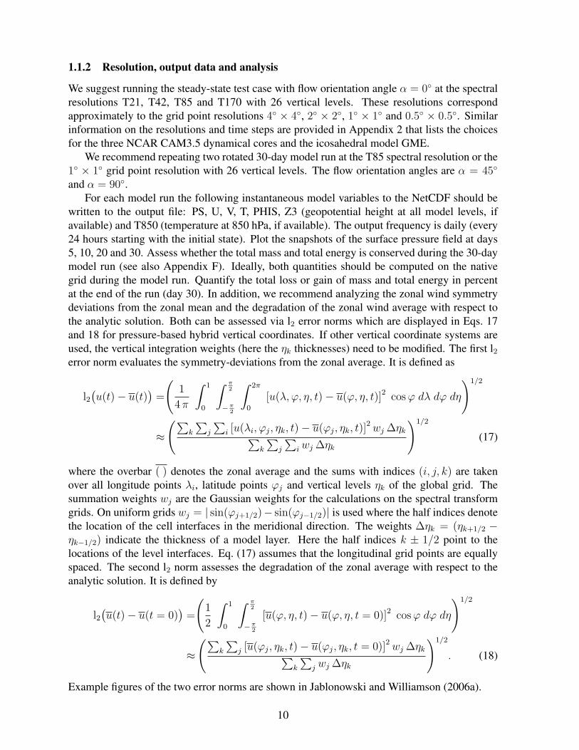
written to the output file: PS, U, V, T, PHIS, Z3 (geopotential height at all model levels, ifavailable) and T850 (temperature at 850 hPa, if available). The output frequency is daily (every24 hours starting with the initial state). Plot the snapshots of the surface pressure field at days5, 10, 20 and 30. Assess whether the total mass and total energy is conserved during the 30-daymodel run (see also Appendix F). Ideally, both quantities should be computed on the nativegrid during the model run. Quantify the total loss or gain of mass and total energy in percentat the end of the run (day 30). In addition, we recommend analyzing the zonal wind symmetrydeviations from the zonal mean and the degradation of the zonal wind average with respect tothe analytic solution. Both can be assessed via l2 error norms which are displayed in Eqs. 17and 18 for pressure-based hybrid vertical coordinates. If other vertical coordinate systems areused, the vertical integration weights (here the ηk thicknesses) need to be modified. The first l2error norm evaluates the symmetry-deviations from the zonal average. It is defined as
l2(u(t)− u(t)
)=
(1
4π
∫ 1
0
∫ π2
−π2
∫ 2π
0
[u(λ, ϕ, η, t)− u(ϕ, η, t)]2 cosϕ dλ dϕ dη
)1/2
≈(∑
k
∑j
∑i [u(λi, ϕj, ηk, t)− u(ϕj, ηk, t)]
2wj ∆ηk∑k
∑j
∑iwj ∆ηk
)1/2
(17)
where the overbar ( ) denotes the zonal average and the sums with indices (i, j, k) are takenover all longitude points λi, latitude points ϕj and vertical levels ηk of the global grid. Thesummation weights wj are the Gaussian weights for the calculations on the spectral transformgrids. On uniform grids wj = | sin(ϕj+1/2)− sin(ϕj−1/2)| is used where the half indices denotethe location of the cell interfaces in the meridional direction. The weights ∆ηk = (ηk+1/2 −ηk−1/2) indicate the thickness of a model layer. Here the half indices k ± 1/2 point to thelocations of the level interfaces. Eq. (17) assumes that the longitudinal grid points are equallyspaced. The second l2 norm assesses the degradation of the zonal average with respect to theanalytic solution. It is defined by
l2(u(t)− u(t = 0)
)=
(1
2
∫ 1
0
∫ π2
−π2
[u(ϕ, η, t)− u(ϕ, η, t = 0)]2 cosϕ dϕ dη
)1/2
≈(∑
k
∑j [u(ϕj, ηk, t)− u(ϕj, ηk, t = 0)]2wj ∆ηk∑
k
∑j wj ∆ηk
)1/2
. (18)
Example figures of the two error norms are shown in Jablonowski and Williamson (2006a).
10

1.2 Baroclinic wave test with tracersA baroclinic wave can be triggered if the initial conditions for the steady-state test (section 1.1)are overlaid with a perturbation. Here a perturbation with a Gaussian profile is selected andcentered at (λc, ϕc) = (π/9, 2π/9) which points to the location (20E,40N). The perturbationoverlays the zonal wind field. The zonal wind perturbation upert is given by
upert(λ, ϕ, η) = up exp(−
( rR
)2 )(19)
with radius R = a/10 and maximum amplitude up = 1 m s−1. It superimposes on the balancedzonal wind field (Eq. (5)) by adding upert to the wind field at each grid point at all model levels.It yields
u(λ, ϕ, η) = u0 cos32 ηv sin2 (2ϕ) + up exp
(−
( rR
)2 )(20)
where the great circle distance r is given by
r = a arccos(
sinϕc sinϕ+ cosϕc cosϕ cos(λ− λc))
. (21)
The corresponding overlaying (ζ ′,δ′ ) perturbations at each level for models in vorticity-divergence form are
ζ ′(λ, ϕ, η) =up
aexp
(−
( rR
)2 )×
tanϕ−
2( aR
)2
arccos(X)sinϕc cosϕ− cosϕc sinϕ cos(λ− λc)√
1−X2
(22)
δ′(λ, ϕ, η) =−2 up a
R2exp
(−
( rR
)2 )arccos(X)
cosϕc sin(λ− λc)√1−X2
(23)
with X =(sinϕc sinϕ + cosϕc cosϕ cos(λ − λc)
). For both singular points (λc, ϕc)
and (λc + π,−ϕc) with X2 = 1, δ′ is identical zero. In addition, ζ ′(λc, ϕc) = up tanϕ/a iswell-defined and limλ→λc+π,ϕ→−ϕc ζ
′ is zero. Similarly, limϕ→±π2ζ ′ is zero at the poles. The
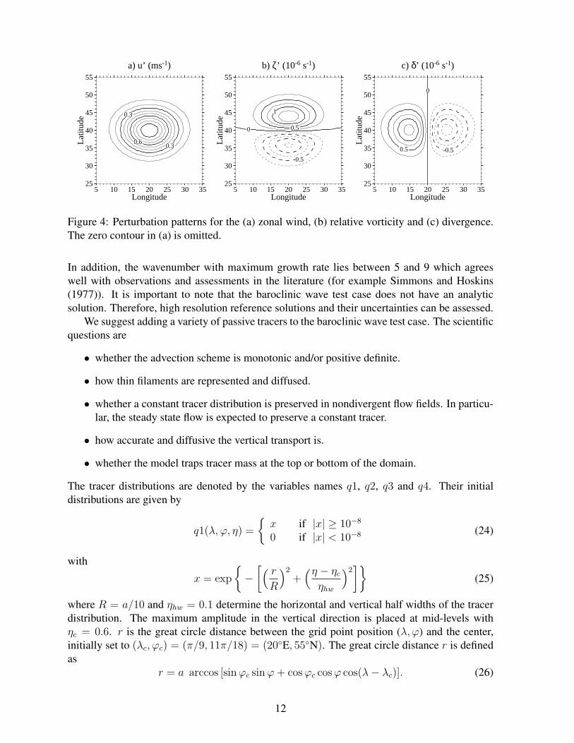
perturbation fields u′, ζ ′ and δ′ are shown in Fig. 4.The evolution of a baroclinic wave in the Northern Hemisphere is triggered when using the
steady-state initial conditions with the overlaid zonal wind perturbation. As before, differenthorizontal resolutions should be assessed to estimate the convergence characteristics. In gen-eral, the baroclinic wave starts growing observably around day 4 and evolves rapidly thereafterwith explosive cyclogenesis at model day 8. The wave train breaks after day 9 and generatesa full circulation in both hemispheres between day 20-30 depending on the model formulation.Therefore, the simulation should cover at least a 10-day time period that captures the initialand rapid development stages of the baroclinic disturbance. If longer time integrations are per-formed (e.g. up to 30 days as in the subsequent examples) the spread of the numerical solutionsincreases noticeably from model day 12 onwards. This indicates the predictability limit of thetest case. Nevertheless, the initial development stages of new systems at the leading edge of thebaroclinic wave train (compare also to Simmons and Hoskins (1979)) are still predicted reliablyuntil day 16.
The baroclinic wave, although idealized, represents very realistic flow features. Strongtemperature fronts develop that are associated with the evolving low and high pressure systems.
11
0.3
0.3
0.6
a) u’ (ms-1)
25
30
35
40
45
50
55L
atitu
de
5 10 15 20 25 30 35Longitude
0 0.5
1
-0.5
b) ζ’ (10-6 s-1)
25
30
35
40
45
50
55
Lat
itude
5 10 15 20 25 30 35Longitude
0
0.5 -0.5
c) δ’ (10-6 s-1)
25
30
35
40
45
50
55
Lat
itude
5 10 15 20 25 30 35Longitude
Figure 4: Perturbation patterns for the (a) zonal wind, (b) relative vorticity and (c) divergence.The zero contour in (a) is omitted.
In addition, the wavenumber with maximum growth rate lies between 5 and 9 which agreeswell with observations and assessments in the literature (for example Simmons and Hoskins(1977)). It is important to note that the baroclinic wave test case does not have an analyticsolution. Therefore, high resolution reference solutions and their uncertainties can be assessed.
We suggest adding a variety of passive tracers to the baroclinic wave test case. The scientificquestions are
• whether the advection scheme is monotonic and/or positive definite.
• how thin filaments are represented and diffused.
• whether a constant tracer distribution is preserved in nondivergent flow fields. In particu-lar, the steady state flow is expected to preserve a constant tracer.
• how accurate and diffusive the vertical transport is.
• whether the model traps tracer mass at the top or bottom of the domain.
The tracer distributions are denoted by the variables names q1, q2, q3 and q4. Their initialdistributions are given by
q1(λ, ϕ, η) =
x if |x| ≥ 10−8
0 if |x| < 10−8 (24)
with
x = exp
−
[( rR
)2
+(η − ηc
ηhw
)2]
(25)
where R = a/10 and ηhw = 0.1 determine the horizontal and vertical half widths of the tracerdistribution. The maximum amplitude in the vertical direction is placed at mid-levels withηc = 0.6. r is the great circle distance between the grid point position (λ, ϕ) and the center,initially set to (λc, ϕc) = (π/9, 11π/18) = (20E, 55N). The great circle distance r is definedas
r = a arccos [sinϕc sinϕ+ cosϕc cosϕ cos(λ− λc)]. (26)
12
A variant of q1 is created when ηc = 0.6 is replaced with ηc = 1. This places the verticalpeak of the tracer distribution at the surface where strong gradients occur during the evolutionof the baroclinic wave. This choice of ηc is defined as tracer field q2.
The other tracer distributions are
q3(λ, ϕ, η) =1
2
[tanh
(3|ϕ| − π
)+ 1
], (27)
q4(λ, ϕ, η) = 1. (28)
Note that q3 only depends on the latitudinal position ϕ and q4 is constant everywhere.
1.2.1 Rotated baroclinic wave initial data set
The steady-state initial data without the perturbation are zonally uniform which favors modelswith orthogonal latitude-longitude or Gaussian grids. Therefore, a rotated version of the initialconditions is suggested. It rotates the computational grid by a flow orientation angle α ∈[0, π/2]. This rotation is also depicted in Fig. E in Appendix 28. For α = 0, the original zonalflow parallel to the equator is recovered, whereas α = π/2 directs the flow field straight overthe poles. The latter setup has the potential to expose filter effects that are associated withpolar filters in latitude-longitude grids. These are frequently used to alleviate the effects of theconverging meridians in spherical geometry. A rotation angle greater zero therefore diminishesthe advantages of the traditional orthogonal grids for zonal flows. In addition, an angle likeα = π/4 challenge the design of cubed-sphere grids that place the corners of the cubed-spherein midlatitudes at ϕ± 45.
Very minor modifications of the model code and initial conditions are necessary for therotated test case. In particular, the change in the model configuration is a rotated Coriolisparameter f(λ, ϕ) that now becomes a 2D field. This is in contrast to the regular 1D settingf(ϕ) = 2Ω sin(ϕ). The rotated Coriolis parameter is
f(λ, ϕ) = 2 Ω [− cosλ cosϕ sinα+ sinϕ cosα]. (29)
The same representation of f is also used in Williamson et al. (1992) for rotated shallow watertest cases.
In addition, the initial conditions for u, v, T and Φs need to be rotated. Following Staniforthand White (2007) the necessary steps are documented in Appendix E and also implemented inthe Fortran test case routines for the initial conditions.
1.2.2 Resolution, output data and analysis
We suggest running the baroclinic wave test case with the flow orientation angle α = 0 at thespectral resolutions T21, T42, T85, T170 and T340 with 26 vertical levels. These resolutionscorrespond approximately to the grid point resolutions 4× 4, 2× 2, 1× 1, 0.5× 0.5 and0.25 × 0.25. Similar information on the resolutions and time steps are provided in Appendix2 that lists the choices for the three NCAR CAM3.5 dynamical cores and the icosahedral modelGME. The integration time is 30 days for T21, T42, T85, T170 and 15 days for T340 to reducethe compute time.
We suggest repeating two rotated 30-day model runs at the T170 spectral resolution orthe 0.5 × 0.5 grid point resolution with 26 vertical levels. If the compute time becomes
13
prohibitive the lower resolution T106 or the 1× 1 grid point resolution with 26 vertical levelsare recommended. The flow orientation angles are α = 45 and α = 90.
For each model run the following instantaneous model variables to the NetCDF should bewritten to the output file: PS, U, V, T, OMEGA, PHIS, Z3 (geopotential height at all modellevels, if available), T850 (temperature at 850 hPa, if available) and all tracers. T850 is avaluable output quantity for at least the first 20 days. At later days the minimum surface pressuremight locally drop below 850 hPa which requires an extrapolation of the temperature to the 850hPa level. The output frequency is daily (every 24 hours starting with the initial state). Plotthe surface pressure, 850 hPa temperature and 850 hPa relative vorticity field at days 7 and 9 inan equidistant cylindrical map projection. An example is provided in Fig. 5 that was computedwith the NCAR CAM3.5.41 Eul model at the resolution T106 with 26 levels. In addition,compute the time sequence at day 15, 20, 25 and 30 of the kinetic energy spectra at 700 hPa.Assess whether the total energy and mass are conserved during the 30-day model run (see alsoAppendix F). Ideally, both quantities should be computed on the native grid during the modelrun. The total energy time series should show the energy difference between the daily (or morefrequent) output and the initial state. In addition, quantify the final energy loss or gain in percent(normalized energy difference).
Interpolate the tracer field q1 at day 9 and 15 to the 700, 600 and 500 hPa levels and plotthe three pressure levels as equidistant cylindrical maps. The tracer field q2 is best evaluated onmodel levels near the surface. We again suggest visualizing at least day 9 and 15. Interpolate thetracer field q3 at day 9 and 15 to the pressure levels 850, 500 and 300 hPa. Plot the three pressurelevels as equidistant cylindrical maps. In addition, evaluate whether the initially constant tracerdistribution q4 shows variations. Assess whether the global tracer masses of q1-q4 are conservedduring the whole forecast period. We will provide NCL (NCAR Command Language) scriptsto help interpolate and evaluate all diagnostic quantities.
The following plots show examples of unrotated and rotated baroclinic wave runs with se-lected tracer distributions. The results were computed with EULT106L26 (see figure captionsfor the details). The noisy contours are due to the Gibb’s ringing effect. The standard diffusioncoefficients were used (see section 2).
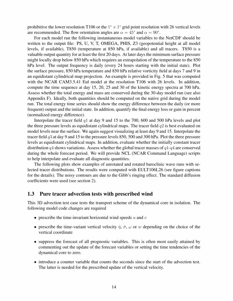
1.3 Pure tracer advection tests with prescribed windThis 3D advection test case tests the transport scheme of the dynamical core in isolation. Thefollowing model code changes are required
• prescribe the time-invariant horizontal wind speeds u and v
• prescribe the time-variant vertical velocity η, σ, ω or w depending on the choice of thevertical coordinate
• suppress the forecast of all prognostic variables. This is often most easily attained bycommenting out the update of the forecast variables or setting the time tendencies of thedynamical core to zero.
• introduce a counter variable that counts the seconds since the start of the advection test.The latter is needed for the prescribed update of the vertical velocity.
14
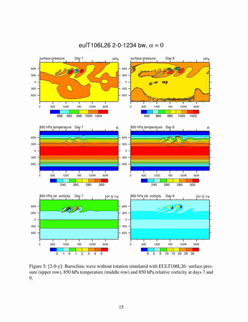
Figure 5: [2-0-y]: Baroclinic wave without rotation simulated with EULT106L26: surface pres-sure (upper row), 850 hPa temperature (middle row) and 850 hPa relative vorticity at days 7 and9.
15
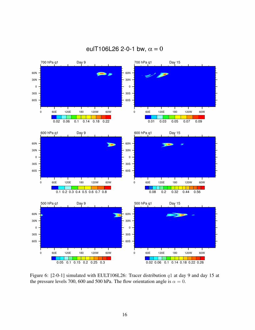
Figure 6: [2-0-1] simulated with EULT106L26: Tracer distribution q1 at day 9 and day 15 atthe pressure levels 700, 600 and 500 hPa. The flow orientation angle is α = 0.
16
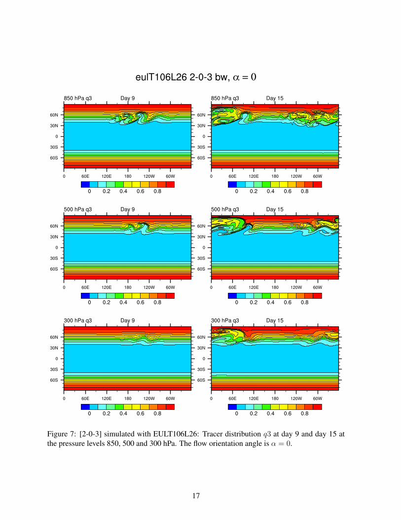
Figure 7: [2-0-3] simulated with EULT106L26: Tracer distribution q3 at day 9 and day 15 atthe pressure levels 850, 500 and 300 hPa. The flow orientation angle is α = 0.
17
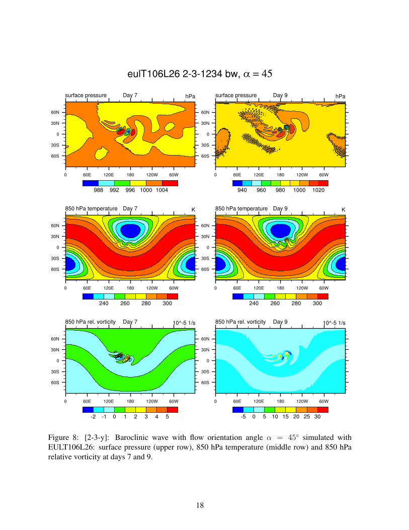
Figure 8: [2-3-y]: Baroclinic wave with flow orientation angle α = 45 simulated withEULT106L26: surface pressure (upper row), 850 hPa temperature (middle row) and 850 hParelative vorticity at days 7 and 9.
18
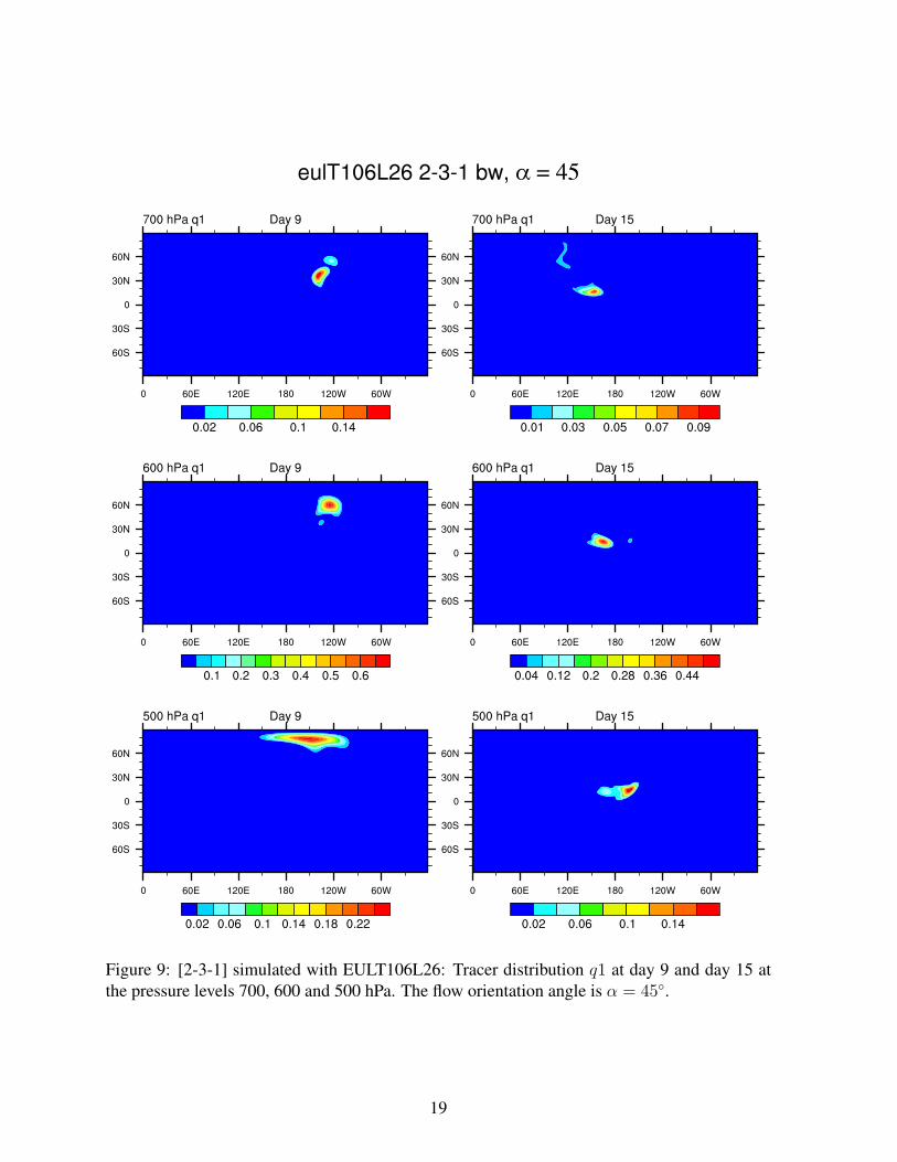
Figure 9: [2-3-1] simulated with EULT106L26: Tracer distribution q1 at day 9 and day 15 atthe pressure levels 700, 600 and 500 hPa. The flow orientation angle is α = 45.
19
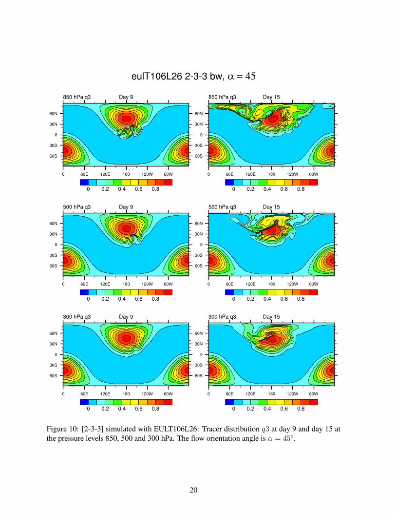
Figure 10: [2-3-3] simulated with EULT106L26: Tracer distribution q3 at day 9 and day 15 atthe pressure levels 850, 500 and 300 hPa. The flow orientation angle is α = 45.
20
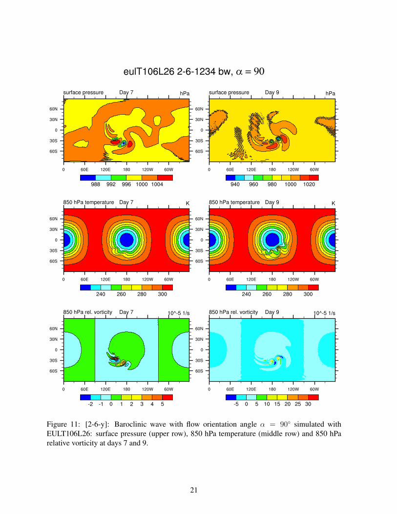
Figure 11: [2-6-y]: Baroclinic wave with flow orientation angle α = 90 simulated withEULT106L26: surface pressure (upper row), 850 hPa temperature (middle row) and 850 hParelative vorticity at days 7 and 9.
21
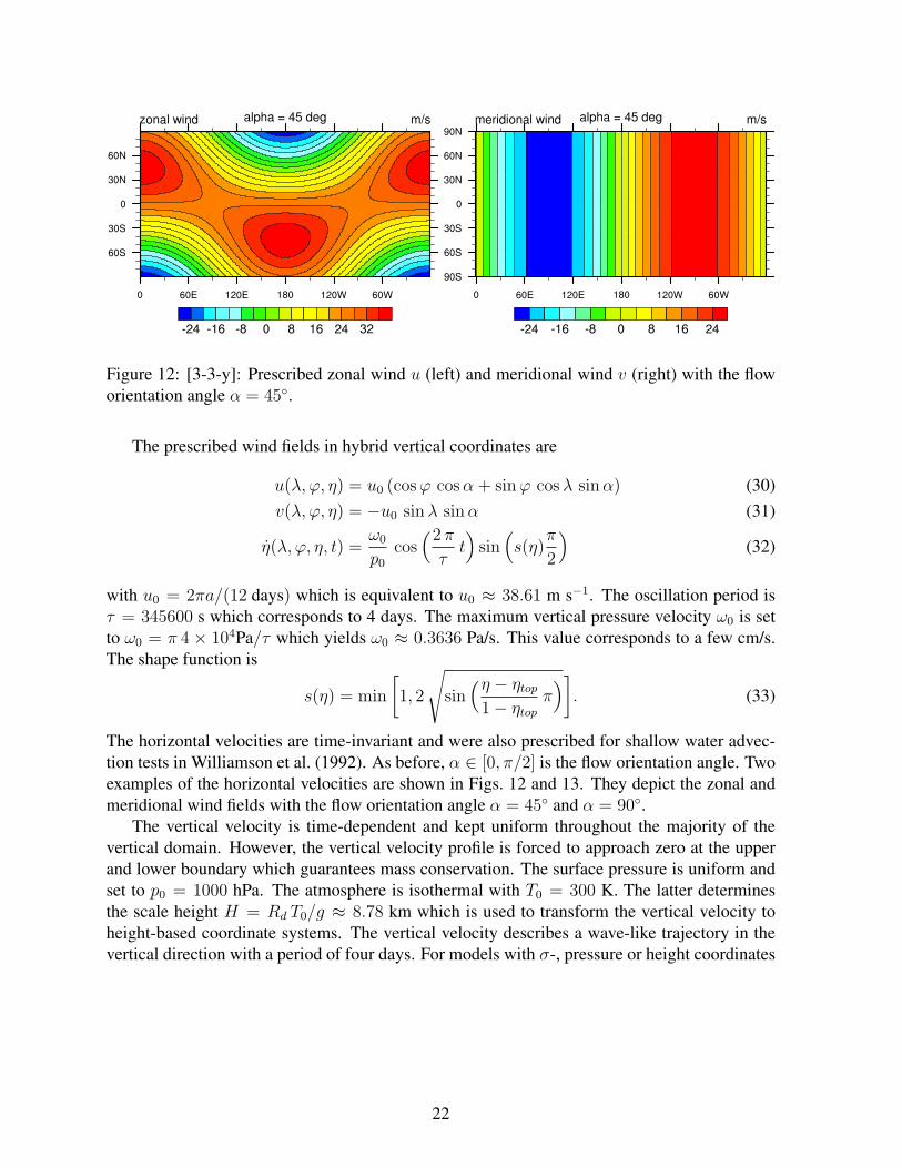
Figure 12: [3-3-y]: Prescribed zonal wind u (left) and meridional wind v (right) with the floworientation angle α = 45.
The prescribed wind fields in hybrid vertical coordinates are
u(λ, ϕ, η) = u0 (cosϕ cosα+ sinϕ cosλ sinα) (30)v(λ, ϕ, η) = −u0 sinλ sinα (31)
η(λ, ϕ, η, t) =ω0
p0
cos(2π
τt)
sin(s(η)
π
2
)(32)
with u0 = 2πa/(12 days) which is equivalent to u0 ≈ 38.61 m s−1. The oscillation period isτ = 345600 s which corresponds to 4 days. The maximum vertical pressure velocity ω0 is setto ω0 = π 4 × 10⁴Pa/τ which yields ω0 ≈ 0.3636 Pa/s. This value corresponds to a few cm/s.The shape function is
s(η) = min
[1, 2
√sin
(η − ηtop
1− ηtop
π)]. (33)
The horizontal velocities are time-invariant and were also prescribed for shallow water advec-tion tests in Williamson et al. (1992). As before, α ∈ [0, π/2] is the flow orientation angle. Twoexamples of the horizontal velocities are shown in Figs. 12 and 13. They depict the zonal andmeridional wind fields with the flow orientation angle α = 45 and α = 90.
The vertical velocity is time-dependent and kept uniform throughout the majority of thevertical domain. However, the vertical velocity profile is forced to approach zero at the upperand lower boundary which guarantees mass conservation. The surface pressure is uniform andset to p0 = 1000 hPa. The atmosphere is isothermal with T0 = 300 K. The latter determinesthe scale height H = Rd T0/g ≈ 8.78 km which is used to transform the vertical velocity toheight-based coordinate systems. The vertical velocity describes a wave-like trajectory in thevertical direction with a period of four days. For models with σ-, pressure or height coordinates
22
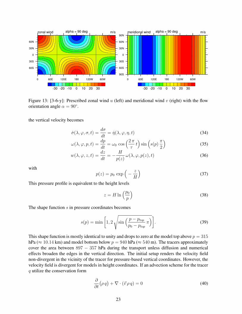
Figure 13: [3-6-y]: Prescribed zonal wind u (left) and meridional wind v (right) with the floworientation angle α = 90.
the vertical velocity becomes
σ(λ, ϕ, σ, t) =dσ
dt= η(λ, ϕ, η, t) (34)
ω(λ, ϕ, p, t) =dp
dt= ω0 cos
(2π
τt)
sin(s(p)
π
2
)(35)
w(λ, ϕ, z, t) =dz
dt= − H
p(z)ω(λ, ϕ, p(z), t) (36)
withp(z) = p0 exp
(− z
H
)(37)
This pressure profile is equivalent to the height levels
z = H ln(p0
p
)(38)
The shape function s in pressure coordinates becomes
s(p) = min
[1, 2
√sin
( p− ptop
p0 − ptop
π)]. (39)
This shape function is mostly identical to unity and drops to zero at the model top above p = 315hPa (≈ 10.14 km) and model bottom below p = 940 hPa (≈ 540 m). The tracers approximatelycover the area between 897 − 357 hPa during the transport unless diffusion and numericaleffects broaden the edges in the vertical direction. The initial setup renders the velocity fieldnon-divergent in the vicinity of the tracer for pressure-based vertical coordinates. However, thevelocity field is divergent for models in height coordinates. If an advection scheme for the tracerq utilize the conservation form
∂
∂t
(ρ q
)+∇ · (~v ρ q) = 0 (40)
23
the following discrete algorithm is recommended to prescribe the pressure p and thereby thedensity ρ. First, we recommend calculating the pressure values p(t2) at the future time t2 =t1 + ∆t where ∆t symbolizes the time step length and t1 is the current time counted in secondssince the start of the advection test. The new pressure values are given by
p(t2) = p(t1) + ∆t ω0 cos[2 π
τ
(t1 +
∆t
2
)]sin
(s(p(t1))
π
2
)(41)
where a time-centered evaluation of the cos-expression is selected. The time dependent densitycan then be computed via the ideal gas law
ρ(t) =p(t)
Rd T0
(42)
with constant temperature T0.This wind field transports the tracer once around the sphere and reaches its initial position
after 12 days. During the revolution the tracer undergoes three wave cycles in the verticaldirection. The initital distribution serves as the analytic solution after 12 days. This allowsthe computation of error norms and thereby an assessment of the numerical diffusion of thetransport scheme.
Two tracer distributions are suggested. The first is a smooth distribution given by
q5(λ, ϕ, z) =1
2
(1 + cos(π d1)
)(43)
with the ellipse-like function
d1 = min
[1,
( rR
)2
+(z − z0
Z
)2]. (44)
As before, r denotes the great circle distance
r = a arccos(
sinϕc sinϕ+ cosϕc cosϕ cos(λ− λc))
(45)
with center position (λc, ϕc) = (3π/2, 0). The vertical center is set to z0 = 4.5 km and thehorizontal and vertical half widths are chosen to be R = a/3 and Z = 1 km. a symbolizes theEarth’s radius.
The second tracer field resembles a slotted ellipse with sharp edges. Such a profile chal-lenges the numerical design of the transport schemes since over- and undershoots are likely tooccur in non-monotonic advection algorithms. The slotted ellipse is given by
q6(λ, ϕ, η) =
1 if d2 ≤ 10 if d2 > 1
(46)
withd2 =
( rR
)2
+(z − z0
Z
)2
(47)
with the same parameters as above. The slot is cut out of the ellipse by the additional condition
q6 = 0 if z > z0 and ϕc − 1
8< ϕ < ϕc +
1
8(48)
24
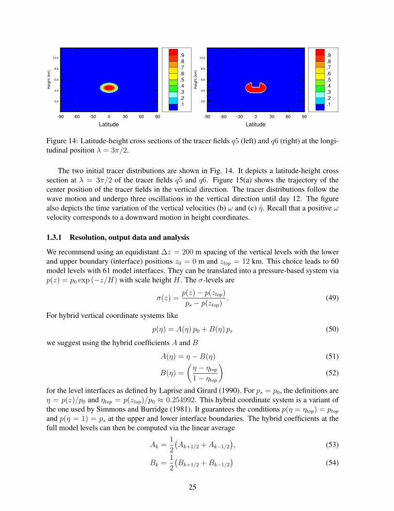
Figure 14: Latitude-height cross sections of the tracer fields q5 (left) and q6 (right) at the longi-tudinal position λ = 3π/2.
The two initial tracer distributions are shown in Fig. 14. It depicts a latitude-height crosssection at λ = 3π/2 of the tracer fields q5 and q6. Figure 15(a) shows the trajectory of thecenter position of the tracer fields in the vertical direction. The tracer distributions follow thewave motion and undergo three oscillations in the vertical direction until day 12. The figurealso depicts the time variation of the vertical velocities (b) ω and (c) η. Recall that a positive ωvelocity corresponds to a downward motion in height coordinates.
1.3.1 Resolution, output data and analysis
We recommend using an equidistant ∆z = 200 m spacing of the vertical levels with the lowerand upper boundary (interface) positions z0 = 0 m and ztop = 12 km. This choice leads to 60model levels with 61 model interfaces. They can be translated into a pressure-based system viap(z) = p0 exp (−z/H) with scale height H . The σ-levels are
σ(z) =p(z)− p(ztop)
ps − p(ztop). (49)
For hybrid vertical coordinate systems like
p(η) = A(η) p0 +B(η) ps (50)
we suggest using the hybrid coefficients A and B
A(η) = η −B(η) (51)
B(η) =
(η − ηtop
1− ηtop
)(52)
for the level interfaces as defined by Laprise and Girard (1990). For ps = p0, the definitions areη = p(z)/p0 and ηtop = p(ztop)/p0 ≈ 0.254992. This hybrid coordinate system is a variant ofthe one used by Simmons and Burridge (1981). It guarantees the conditions p(η = ηtop) = ptop
and p(η = 1) = ps at the upper and lower interface boundaries. The hybrid coefficients at thefull model levels can then be computed via the linear average
Ak =1
2
(Ak+1/2 + Ak−1/2
), (53)
Bk =1
2
(Bk+1/2 +Bk−1/2
)(54)
25
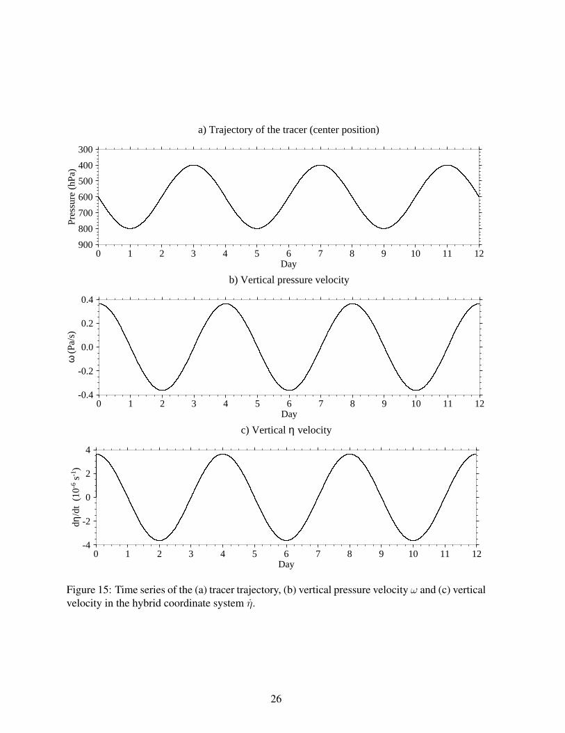
a) Trajectory of the tracer (center position)
300
400
500
600
700
800
900
Pres
sure
(hP
a)
0 1 2 3 4 5 6 7 8 9 10 11 12Day
b) Vertical pressure velocity
-0.4
-0.2
0.0
0.2
0.4
ω (
Pa/s
)
0 1 2 3 4 5 6 7 8 9 10 11 12Day
c) Vertical η velocity
-4
-2
0
2
4
dη/d
t (1
0-6 s
-1)
0 1 2 3 4 5 6 7 8 9 10 11 12Day
Figure 15: Time series of the (a) tracer trajectory, (b) vertical pressure velocity ω and (c) verticalvelocity in the hybrid coordinate system η.
26
where the index k denotes the discrete full model level which is surrounded by the two inter-face levels shown with half indices. The linear average guarantees that vertical differencingoperations conserve energy. Note that some models (Majewski et al. 2002) use the alternativedefinition of Eq. (50)
p(η) = A(η) + B(η) ps. (55)
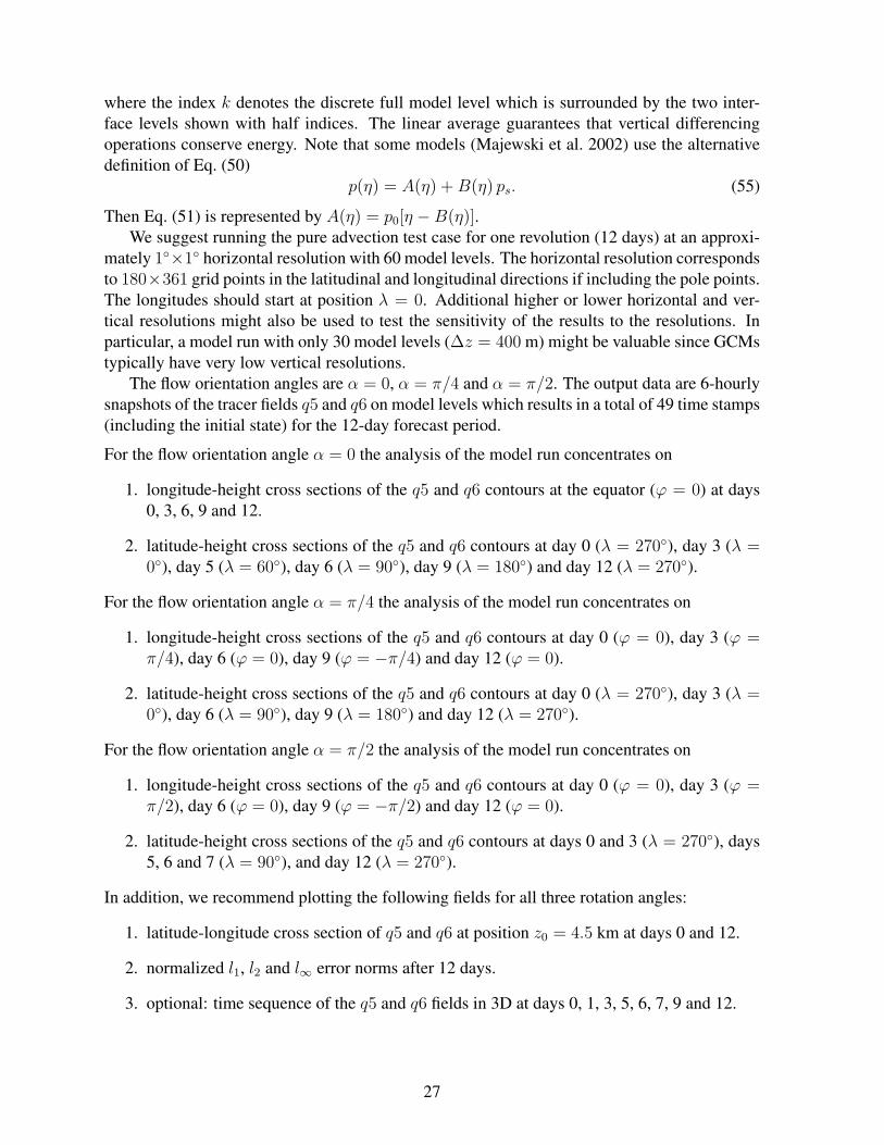
Then Eq. (51) is represented by A(η) = p0[η −B(η)].We suggest running the pure advection test case for one revolution (12 days) at an approxi-
mately 1×1 horizontal resolution with 60 model levels. The horizontal resolution correspondsto 180×361 grid points in the latitudinal and longitudinal directions if including the pole points.The longitudes should start at position λ = 0. Additional higher or lower horizontal and ver-tical resolutions might also be used to test the sensitivity of the results to the resolutions. Inparticular, a model run with only 30 model levels (∆z = 400 m) might be valuable since GCMstypically have very low vertical resolutions.
The flow orientation angles are α = 0, α = π/4 and α = π/2. The output data are 6-hourlysnapshots of the tracer fields q5 and q6 on model levels which results in a total of 49 time stamps(including the initial state) for the 12-day forecast period.
For the flow orientation angle α = 0 the analysis of the model run concentrates on
1. longitude-height cross sections of the q5 and q6 contours at the equator (ϕ = 0) at days0, 3, 6, 9 and 12.
2. latitude-height cross sections of the q5 and q6 contours at day 0 (λ = 270), day 3 (λ =0), day 5 (λ = 60), day 6 (λ = 90), day 9 (λ = 180) and day 12 (λ = 270).
For the flow orientation angle α = π/4 the analysis of the model run concentrates on
1. longitude-height cross sections of the q5 and q6 contours at day 0 (ϕ = 0), day 3 (ϕ =π/4), day 6 (ϕ = 0), day 9 (ϕ = −π/4) and day 12 (ϕ = 0).
2. latitude-height cross sections of the q5 and q6 contours at day 0 (λ = 270), day 3 (λ =0), day 6 (λ = 90), day 9 (λ = 180) and day 12 (λ = 270).
For the flow orientation angle α = π/2 the analysis of the model run concentrates on
1. longitude-height cross sections of the q5 and q6 contours at day 0 (ϕ = 0), day 3 (ϕ =π/2), day 6 (ϕ = 0), day 9 (ϕ = −π/2) and day 12 (ϕ = 0).
2. latitude-height cross sections of the q5 and q6 contours at days 0 and 3 (λ = 270), days5, 6 and 7 (λ = 90), and day 12 (λ = 270).
In addition, we recommend plotting the following fields for all three rotation angles:
1. latitude-longitude cross section of q5 and q6 at position z0 = 4.5 km at days 0 and 12.
2. normalized l1, l2 and l∞ error norms after 12 days.
3. optional: time sequence of the q5 and q6 fields in 3D at days 0, 1, 3, 5, 6, 7, 9 and 12.
27
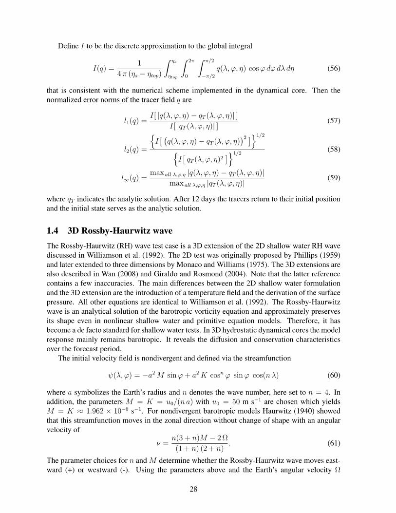
Define I to be the discrete approximation to the global integral
I(q) =1
4π (ηs − ηtop)
∫ ηs
ηtop
∫ 2π
0
∫ π/2
−π/2
q(λ, ϕ, η) cosϕdϕdλ dη (56)
that is consistent with the numerical scheme implemented in the dynamical core. Then thenormalized error norms of the tracer field q are
l1(q) =I[ |q(λ, ϕ, η)− qT (λ, ϕ, η)| ]
I[ |qT (λ, ϕ, η)| ] (57)
l2(q) =
I[ (q(λ, ϕ, η)− qT (λ, ϕ, η)
)2 ]1/2
I[qT (λ, ϕ, η)2
]1/2(58)
l∞(q) =max all λ,ϕ,η |q(λ, ϕ, η)− qT (λ, ϕ, η)|
max all λ,ϕ,η |qT (λ, ϕ, η)| (59)
where qT indicates the analytic solution. After 12 days the tracers return to their initial positionand the initial state serves as the analytic solution.
1.4 3D Rossby-Haurwitz waveThe Rossby-Haurwitz (RH) wave test case is a 3D extension of the 2D shallow water RH wavediscussed in Williamson et al. (1992). The 2D test was originally proposed by Phillips (1959)and later extended to three dimensions by Monaco and Williams (1975). The 3D extensions arealso described in Wan (2008) and Giraldo and Rosmond (2004). Note that the latter referencecontains a few inaccuracies. The main differences between the 2D shallow water formulationand the 3D extension are the introduction of a temperature field and the derivation of the surfacepressure. All other equations are identical to Williamson et al. (1992). The Rossby-Haurwitzwave is an analytical solution of the barotropic vorticity equation and approximately preservesits shape even in nonlinear shallow water and primitive equation models. Therefore, it hasbecome a de facto standard for shallow water tests. In 3D hydrostatic dynamical cores the modelresponse mainly remains barotropic. It reveals the diffusion and conservation characteristicsover the forecast period.
The initial velocity field is nondivergent and defined via the streamfunction
ψ(λ, ϕ) = −a2M sinϕ+ a2K cosn ϕ sinϕ cos(nλ) (60)
where a symbolizes the Earth’s radius and n denotes the wave number, here set to n = 4. Inaddition, the parameters M = K = u0/(n a) with u0 = 50 m s−1 are chosen which yieldsM = K ≈ 1.962 × 10⁻⁶ s−1. For nondivergent barotropic models Haurwitz (1940) showedthat this streamfunction moves in the zonal direction without change of shape with an angularvelocity of
ν =n(3 + n)M − 2 Ω
(1 + n) (2 + n). (61)
The parameter choices for n and M determine whether the Rossby-Haurwitz wave moves east-ward (+) or westward (-). Using the parameters above and the Earth’s angular velocity Ω
28
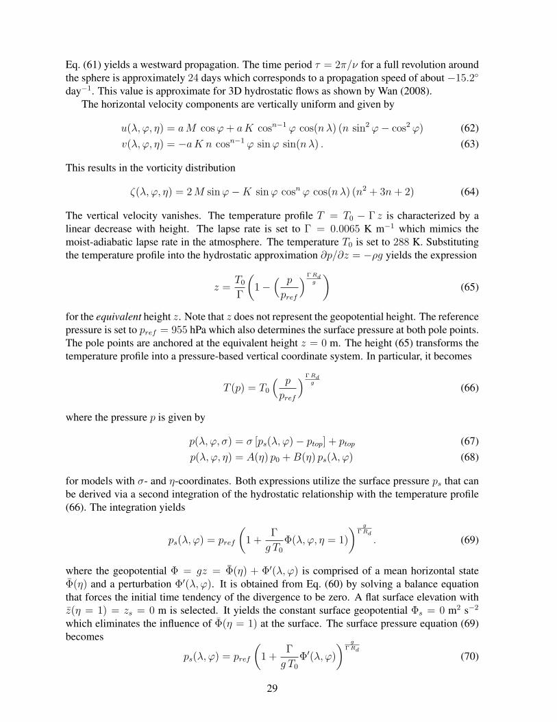
Eq. (61) yields a westward propagation. The time period τ = 2π/ν for a full revolution aroundthe sphere is approximately 24 days which corresponds to a propagation speed of about −15.2
day−1. This value is approximate for 3D hydrostatic flows as shown by Wan (2008).The horizontal velocity components are vertically uniform and given by
u(λ, ϕ, η) = aM cosϕ+ aK cosn−1 ϕ cos(nλ) (n sin2 ϕ− cos2 ϕ) (62)v(λ, ϕ, η) = −aK n cosn−1 ϕ sinϕ sin(nλ) . (63)
This results in the vorticity distribution
ζ(λ, ϕ, η) = 2M sinϕ−K sinϕ cosn ϕ cos(nλ) (n2 + 3n+ 2) (64)
The vertical velocity vanishes. The temperature profile T = T0 − Γ z is characterized by alinear decrease with height. The lapse rate is set to Γ = 0.0065 K m−1 which mimics themoist-adiabatic lapse rate in the atmosphere. The temperature T0 is set to 288 K. Substitutingthe temperature profile into the hydrostatic approximation ∂p/∂z = −ρg yields the expression
z =T0
Γ
(1−
( p
pref
)Γ Rdg
)(65)
for the equivalent height z. Note that z does not represent the geopotential height. The referencepressure is set to pref = 955 hPa which also determines the surface pressure at both pole points.The pole points are anchored at the equivalent height z = 0 m. The height (65) transforms thetemperature profile into a pressure-based vertical coordinate system. In particular, it becomes
T (p) = T0
( p
pref
)Γ Rdg
(66)
where the pressure p is given by
p(λ, ϕ, σ) = σ [ps(λ, ϕ)− ptop] + ptop (67)p(λ, ϕ, η) = A(η) p0 +B(η) ps(λ, ϕ) (68)
for models with σ- and η-coordinates. Both expressions utilize the surface pressure ps that canbe derived via a second integration of the hydrostatic relationship with the temperature profile(66). The integration yields
ps(λ, ϕ) = pref
(1 +
Γ
g T0
Φ(λ, ϕ, η = 1)
) gΓ Rd
. (69)
where the geopotential Φ = gz = Φ(η) + Φ′(λ, ϕ) is comprised of a mean horizontal stateΦ(η) and a perturbation Φ′(λ, ϕ). It is obtained from Eq. (60) by solving a balance equationthat forces the initial time tendency of the divergence to be zero. A flat surface elevation withz(η = 1) = zs = 0 m is selected. It yields the constant surface geopotential Φs = 0 m2 s−2
which eliminates the influence of Φ(η = 1) at the surface. The surface pressure equation (69)becomes
ps(λ, ϕ) = pref
(1 +
Γ
g T0
Φ′(λ, ϕ)
) gΓ Rd
(70)
29
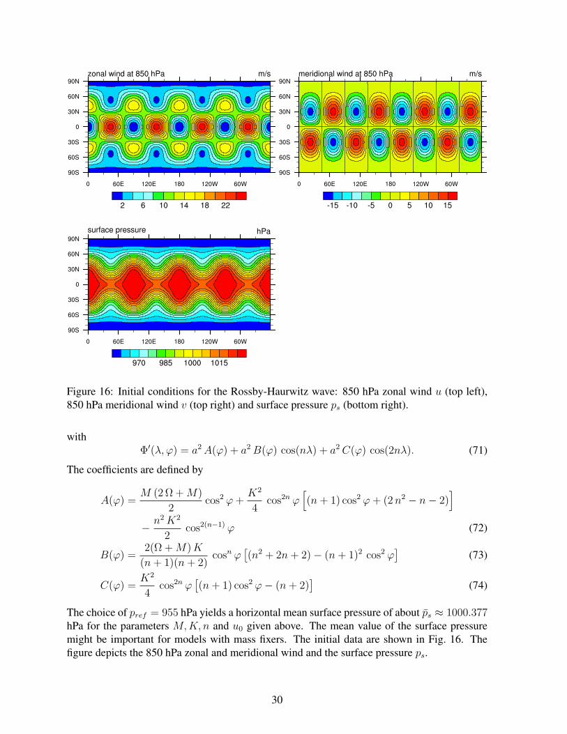
Figure 16: Initial conditions for the Rossby-Haurwitz wave: 850 hPa zonal wind u (top left),850 hPa meridional wind v (top right) and surface pressure ps (bottom right).
withΦ′(λ, ϕ) = a2A(ϕ) + a2B(ϕ) cos(nλ) + a2C(ϕ) cos(2nλ). (71)
The coefficients are defined by
A(ϕ) =M (2 Ω +M)
2cos2 ϕ+
K2
4cos2n ϕ
[(n+ 1) cos2 ϕ+ (2n2 − n− 2)
]
− n2K2
2cos2(n−1) ϕ (72)
B(ϕ) =2(Ω +M)K
(n+ 1)(n+ 2)cosn ϕ
[(n2 + 2n+ 2)− (n+ 1)2 cos2 ϕ
](73)
C(ϕ) =K2
4cos2n ϕ
[(n+ 1) cos2 ϕ− (n+ 2)
](74)
The choice of pref = 955 hPa yields a horizontal mean surface pressure of about ps ≈ 1000.377hPa for the parameters M,K, n and u0 given above. The mean value of the surface pressuremight be important for models with mass fixers. The initial data are shown in Fig. 16. Thefigure depicts the 850 hPa zonal and meridional wind and the surface pressure ps.
30
1.4.1 Resolution, output data and analysis
We recommend running the Rossby-Haurwitz test case for 30 days at an approximately 1 ×1 horizontal resolution with 26 vertical levels as outlined in Appendix C. This horizontalresolution corresponds to 181 × 360 grid points in the latitudinal and longitudinal directions ifincluding the pole points. If height-based vertical coordinates are used the model top must liebelow ztop = T0/Γ = 44.307 km.
The output data are daily snapshots of the fields U, V, OMEGA, T, PS, PHIS and Z3 (ifavailable) on model levels. In addition, the output variables T850, T300, U850, U200, V850,V200, OMEGA850, OMEGA500 and Z500 should be selected (if available). The analysis ofthe model run concentrates on
1. 500 hPa geopotential height Z500 contours at days 5, 10, 15 and 30 on an equidistantcylindrical latitude-longitude map.
2. U, V, T and the OMEGA fields at p = 850 hPa at days 5, 10, 15 and 30 on equidistantcylindrical latitude-longitude maps. The contour spacings are 4 m s −1 for U and V, and0.1 K for T.
3. equidistant cylindrical latitude-longitude map of PS at day 5, 10, 15 and 30. The contourspacing is 10 hPa.
4. time series of the domain integrated total energy (see Appendix F). Plot the energy dif-ference between the daily (or more frequent) output and the initial state. In addition,quantify the final energy loss or gain in percent (normalized energy difference).
5. evaluation of the Rossby-Haurwitz wave without explicit horizontal diffusion (if applica-ble). Are the simulations computationally stable?
6. effects of enhanced explicit diffusion near the model top (if applicable). Plot U, V, T atthe second model level (p ≈ 7.3 hPa) on equidistant cylindrical latitude-longitude maps.
7. the symmetry of the wave in the Northern and Southern hemisphere.
8. whether the wave breaks down over the 30-day forecast period and if yes when?
The geopotential height is given by∫ z
zs
dz′ = −Rd
g
∫ p
ps
Td(ln p′) (75)
which can be approximated in the discrete system as
zm = zs +Rd
g
m∑
k=Kmax
Tk∆(ln pk)
= zs +Rd
g
m∑
k=Kmax
Tk(ln pk+1/2 − ln pk−1/2) (76)
This expression results in the geopotential height zm at level index m < Kmax. The summationstarts near the surface with maximum level number Kmax with decreasing level index k in the
31
upward direction. The half-indices describe the interface levels. zs = Φs/g is the surfaceelevation which is zero in this test case. For the computation of the geopotential height at afixed pressure surface p500 = 500 hPa the summation over the full model levels stops at theinterface level that lies just below p500. This interface level is denoted by index m + 1/2. Theremaining fractional contribution upward of interface level m + 1/2 is added via the last termin
zp = zs +Rd
g
m+1∑
k=Kmax
[Tk(ln pk+1/2 − ln pk−1/2)
]+ Tm(ln pm+1/2 − ln p500). (77)
The 850 hPa wind velocities and temperature can be derived via a linear interpolation in ln pcoordinates that takes the two surrounding model levels into account.
Snapshots of the output data at day 15 are presented in Fig. 17. The figure shows the 850hPa zonal wind, meridional wind, temperature and vertical velocity fields as well as the 500hPa geopotential height and surface pressure. These model results were computed with theCAM3.5.41 verison of the NCAR Finite Volume (FV) dynamical core at the resolution 1 × 1
with 26 hybrid levels.
1.5 Mountain-induced Rossby wave trainThe definition of the mountain-induced Rossby wave train closely resembles the descriptionof the initial conditions by Tomita and Sato (2004). The main difference is the derivationof the surface pressure for hydrostatic conditions as considered here. The simulation startsfrom smooth isothermal initial conditions that are a balanced analytic solution to the primitiveequations. They are also a solution to the non-hydrostatic shallow atmosphere equation set. Anidealized mountain then triggers the evolution of a Rossby wave train over the course of 15days. We recommend integrating the models until day 30 to investigate the further evolution ofthe circulation.
The horizontal wind components are prescribed as
u(λ, ϕ, η) = u0 cosϕ (78)v(λ, ϕ, η) = 0 m s−1. (79)
The amplitude of the zonal wind u0 is set to 20 m s−1, the vertical velocity vanishes. Thetemperature is isothermal and given by T (λ, ϕ, η) = T0 = 288 K. This yields the constantBrunt-Vaisala frequency
N =
√g2
cp T0
≈ 0.0182 s−1. (80)
The gravitational acceleration g and specific heat at constant pressure cp are listed in AppendixG. An idealized bell-shape mountain is introduced via the surface geopotential
Φs(λ, ϕ) = gzs = gh0 exp
[−
(rd
)2]
(81)
where h0 = 2000 m determines the peak height of the mountain and d = 1500 km is the halfwidth of the Gaussian mountain profile. As before, r is defined as the great circle distance
r = a arccos [sinϕc sinϕ+ cosϕc cosϕ cos(λ− λc)] (82)
32
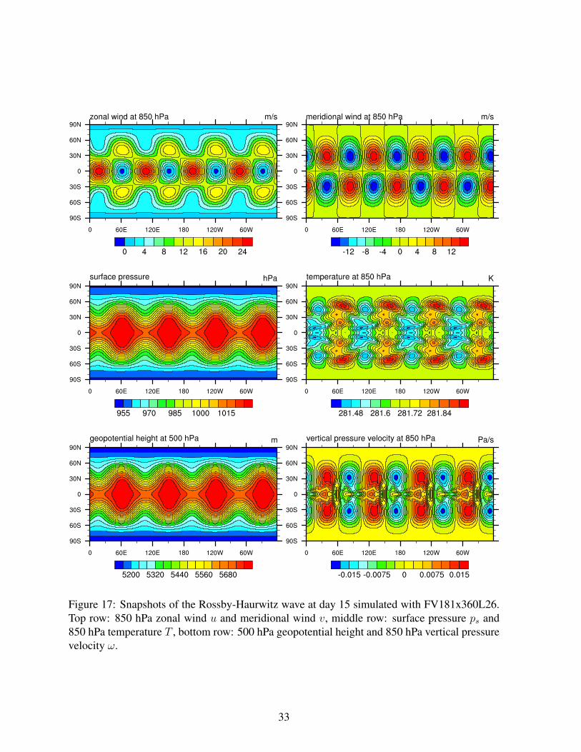
Figure 17: Snapshots of the Rossby-Haurwitz wave at day 15 simulated with FV181x360L26.Top row: 850 hPa zonal wind u and meridional wind v, middle row: surface pressure ps and850 hPa temperature T , bottom row: 500 hPa geopotential height and 850 hPa vertical pressurevelocity ω.
33
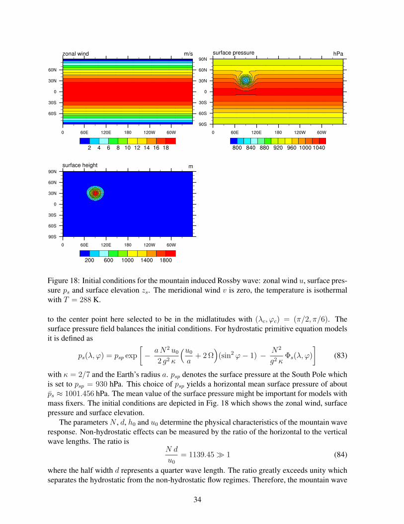
Figure 18: Initial conditions for the mountain induced Rossby wave: zonal wind u, surface pres-sure ps and surface elevation zs. The meridional wind v is zero, the temperature is isothermalwith T = 288 K.
to the center point here selected to be in the midlatitudes with (λc, ϕc) = (π/2, π/6). Thesurface pressure field balances the initial conditions. For hydrostatic primitive equation modelsit is defined as
ps(λ, ϕ) = psp exp
[− aN2 u0
2 g2 κ
(u0
a+ 2 Ω
)(sin2 ϕ− 1) − N2
g2 κΦs(λ, ϕ)
](83)
with κ = 2/7 and the Earth’s radius a. psp denotes the surface pressure at the South Pole whichis set to psp = 930 hPa. This choice of psp yields a horizontal mean surface pressure of aboutps ≈ 1001.456 hPa. The mean value of the surface pressure might be important for models withmass fixers. The initial conditions are depicted in Fig. 18 which shows the zonal wind, surfacepressure and surface elevation.
The parameters N , d, h0 and u0 determine the physical characteristics of the mountain waveresponse. Non-hydrostatic effects can be measured by the ratio of the horizontal to the verticalwave lengths. The ratio is
N d
u0
= 1139.45 À 1 (84)
where the half width d represents a quarter wave length. The ratio greatly exceeds unity whichseparates the hydrostatic from the non-hydrostatic flow regimes. Therefore, the mountain wave
34
response is hydrostatic. In addition, the non-linear effects are measured by the gravity wavestrength Nh normalized by the base state wind
N h
u0
= 1.82. (85)
This is the inverse Froude number that is a more than twice the critical value of 0.85 for whicha flow transition is expected. The mountain therefore triggers a nonlinear finite-amplitudewave response. At mid-levels it resembles the barotropic mountain wave train described inWilliamson et al. (1992).
1.5.1 Resolution, output data and analysis
We recommend running the Rossby wave train test for 30 days at an approximately 1×1 hor-izontal resolution with 26 vertical levels as outlined in Appendix C. This horizontal resolutioncorresponds to 181 × 360 grid points in the latitudinal and longitudinal directions if includingthe pole points.
The output data are daily snapshots of the fields U, V, OMEGA, T, PS, PHIS and Z3 onmodel levels. In addition, the output variables T300, U200, V200, OMEGA500, Z700, Z500and Z300 should be selected (if available). The analysis of the model run concentrates on
1. U, V, T, OMEGA and geopotential height at 700 hPa km at days 5, 10, 15, 20 and 25on equidistant cylindrical latitude-longitude maps. Contour intervals are 5 m/s for U andV, 3 K for T, and 100 m for the geopotential height. We also recommend plotting thetemperature at 300 hPa with a 1K contour interval.
2. OMEGA longitude-pressure cross section at 45N at day 15.
3. time series of the domain integrated total energy. Plot the energy difference between thedaily (or more frequent) output and the initial state. In addition, quantify the final energyloss or gain in percent (normalized energy difference).
The computation of the geopotential height and the vertical interpolations of U, V, T andOMEGA to the 700 hPa level are outlined in section 1.4. The computation of the geopoten-tial and interpolations can also be a post-processing step which is e.g. supported by the NCARCommand Language NCL.
Snapshots of the 700 hPa geopotential height and 700 hPa temperature fields at days 5, 15and 25 are presented in Fig. 19. In addition, Fig. 20 shows snapshots of the zonal and meridionalwind field at 700 hPa. The results were computed with the CAM3.5.41 version of the NCARFinite Volume (FV) dynamical core at the resolution 1 × 1 with 26 hybrid levels.
1.6 Gravity waves with and without the Earth’s rotationThis test case explores with propagation of gravity waves in the spherical domain. Two variantsof the test case are considered. First, the Earth’s rotation Ω and thereby the Coriolis parameterf = 2Ω sinϕ are set to zero which assesses the propagation of pure gravity waves. Second, theEarth’s rotation and Coriolis parameter are retained that allows the analysis of inertia-gravity
35

Figure 19: Snapshots of the mountain induced Rossby wave at days 5, 15 and 25 simulated withFV181x360L26. Left column: 700 hPa geopotential height, right column: 700 hPa temperatureT .
36
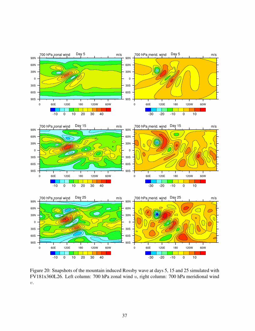
Figure 20: Snapshots of the mountain induced Rossby wave at days 5, 15 and 25 simulated withFV181x360L26. Left column: 700 hPa zonal wind u, right column: 700 hPa meridional windv.
37
waves. The initial data trigger large-scale and thereby hydrostatic waves that propagate outwardin concentric circles. The wind speeds are given by
u = u0 cosϕ
v = 0 m s−1
which results in
ζ =2 u0
asinϕ (86)
δ = 0 s−1
for models in vorticity-divergence form. a denotes the Earth’s radius and u0 is the maximumwind amplitude which is set to either 0 or 40 m s−1 depending on the chosen test case variant.In addition, the vertical velocity and and surface geopotential Φs are set to zero. The surfacepressure field is balanced for the zonally symmetric (unperturbed) state and given by
ps(λ, ϕ) = peq exp
[− aN2 u0
2 g2 κ
(u0
a+ 2 Ω
)sin2 ϕ
](87)
with κ = Rd/cp = 2/7. The values for the gas constant Rd, specific heat at constant pressurecp and the gravitational acceleration g are listed in Appendix G. N2 symbolizes the squaredBrunt-Vaisala frequency. peq denotes the surface pressure at the equator which is set to peq =p0 = 1000 hPa. Note that the surface pressure is constant with ps = peq = p0 for initial statesat rest with u0 = 0 m s−1.
The initial temperature field is given by analytic expressions for models with pressure-basedor height-based vertical coordinates. In case of ps = p0 the pressure p and height z positionsare interchangeable and represented by
p(z) = p0
[(1− S
T0
)+S
T0
exp(− N2z
g
)] cpRd
(88)
z(p) = − g
N2ln
[T0
S
( p
p0
)κ
− 1
+ 1
](89)
with the parameter S = g2/(cpN2). S has temperature units. T0 represents a reference temper-
ature at the surface which is set to T0 = 300 K. N denotes the Brunt-Vaisala frequency that iseither chosen to be
N = 0.01 s−1 or
N =
√( g2
cpT0
)≈ 0.01786 s−1 (90)
depending on the test case variant. The latter corresponds to isothermal background conditionswith temperature T0. The pressure-height relationship shown in Eqs. (88) and (89) is not exactfor the test case variant [6-2-0] with ps 6= p0. In the isothermal T = T0 case with Brunt-Vaisalafrequency (90) the pressure-height relationship for ps 6= p0 becomes
p(λ, ϕ, z) = ps(λ, ϕ) exp(− g z
Rd T0
)(91)
z(λ, ϕ, p) =Rd T0
gln
(ps(λ, ϕ)
p
)(92)
38
However, to simplify the test setup we suggest utilizing Eqs. (88) and (89) for all gravity wavevariants. We note that this implies an approximation for the temperature initialization in [6-2-0].
The initial temperature data are composed of a horizontally uniform background field that isoverlaid by a large scale temperature perturbation. This approach has also been used by Tomitaand Sato (2004). In particular, the temperature perturbation is defined in terms of the potentialtemperature. The definitions of the initial temperature fields are
T (λ, ϕ, z) = Θ(λ, ϕ, z)(p(z)p0
)κ
(93)
T (λ, ϕ, p) = Θ(λ, ϕ, p)( p
p0
)κ
(94)
where Θ(λ, ϕ, z) and Θ(λ, ϕ, p) are composed of the mean state Θ in the vertical direction anda 3D perturbation Θ′. The analytic expression for the height-based potential temperature are
Θ(λ, ϕ, z) = Θ(z) + Θ′(λ, ϕ, z)
= T0 exp(N2z
g
)+ ∆Θ s(λ, ϕ) sin
(2π z
Lz
)(95)
For pressure-based vertical coordinates, the potential temperature field is given as
Θ(λ, ϕ, p) = Θ(p) + Θ′(λ, ϕ, p)
=T0
T0
S
((pp0
)κ − 1)
+ 1+ ∆Θ s(λ, ϕ) sin
(2π z(p)
Lz
). (96)
The horizontal shape function s(λ, ϕ) resembles the cosine hill definition documented inWilliamson et al. (1992) (shallow water test case 1). It is defined as
s(λ, ϕ) =
0.5
(1 + cos(πr/R)
)if r < R
0 if r ≥ R(97)
with R = a/3. r is the great circle distance between a position (λ, ϕ) and the center of thecosine bell, initially set to (λc, ϕc) = (π, 0). The great circle distance r is defined as
r = a arccos [sinϕc sinϕ+ cosϕc cosϕ cos(λ− λc)] (98)
The maximum potential temperature amplitude is ∆Θ = 10 K and the vertical wave length ofthe perturbation is set to Lz = 20 km. We recommend setting the height of the model top toztop = 10 km which corresponds to half a wave length ztop = Lz/2. Using N = 0.01 s−1 thetop level (interface) pressure then yields ptop = p(ztop) ≈ 273.819 hPa according to Eq. (88).When using isothermal conditions with N = 0.01786 s−1 the position of the top level interfacepressure is ptop = p(ztop) ≈ 320.213 hPa. Here, both positions of the model tops are computedfor ps = p0. We also recommend using these model tops for test variant [6-2-0] with varyingsurface pressure.
For completeness, the representation of the mean temperature profiles T are
T (z) = exp(N2z
g
)(T0 − S
)+ S (99)
T (p) =T0
(pp0
)κ
T0
S
((pp0
)κ − 1)
+ 1(100)
39
which are incorporated above in Eqs. 93 and 94. Note that
Θ(z) = T0 exp(N2z
g
)
= T (z)( p0
p(z)
)κ
(101)
despite the apparent differences in the analytic expressions. The equivalency can easily beconfirmed analytically for isothermal conditions.
We suggest using an approximately equidistant ∆z = 500 m spacing of the vertical levels.Strictly speaking (for pressure-based vertical coordinates), the levels are only truly equidistantin height without the temperature perturbation and constant ps = p0. Placing the model top atztop = 10 km leads to 20 full model levels and 21 interface levels. The interface levels includethe lower and upper boundaries z0 = 0 m and ztop. The level spacing can be translated into apressure-based system via Eq. (88) or Eq. (92). The σ-levels are
σ(z) =p(z)− p(ztop)
ps − p(ztop)(102)
with constant p(ztop) as determined above.For hybrid vertical coordinate systems like
p(η) = A(η) p0 +B(η) ps (103)
we recommend using the hybrid coefficients A and B
A(η) = η −B(η) (104)
B(η) =
(η − ηtop
1− ηtop
)c
(105)
for the interface levels as suggested by Laprise and Girard (1990). For ps = p0 and N = 0.01s−1, the definitions are η = p(z)/ps and ηtop = p(ztop)/ps ≈ 0.273819. For N = 0.0178 s−1 themodel top interface level lies at ηtop = p(ztop)/ps ≈ 0.320213. We recommend also using thesemodel top positions for test variant [6-2-0] with ps 6= p0 which will lead to slight deviationsfrom the equidistant spacing in hybrid coordinates. The exponent c determines the smoothnessof the transition between the σ-coordinate at low levels to the pressure coordinate near the upperboundary. We recommend choosing c = 1 which closely resembles the σ-system. This hybridcoordinate system is a variant of the one used by Simmons and Burridge (1981). It guaranteesthe conditions p(η = ηtop) = ptop and p(η = 1) = ps at the upper and lower boundaries. Thehybrid coefficients at the full model levels can then be computed via the linear average
Ak =1
2
(Ak+1/2 + Ak−1/2
), (106)
Bk =1
2
(Bk+1/2 +Bk−1/2
)(107)
where the index k denotes the discrete full model level which is surrounded by the two interfacelevels shown with half indices. The linear interpolation guarantees that vertical differencing
40
operations conserve energy. Note that some models (Majewski et al. 2002) use the alternativedefinition of Eq. (103)
p(η) = A(η) + B(η) ps. (108)
Then Eq. (104) is represented by A(η) = p0[η −B(η)].The gravity wave response is nearly linear and hydrostatic and therefore determined by the
dispersion relation
ν2 = f 2 +N2 k2 + l2
m2(109)
where ν indicates the frequency. The zonal, meridional and vertical wave numbers are definedas k = 2πL−1
x , l = 2πL−1y and m = 2πL−1
z where Lx, Ly and Lz represent the zonal andmeridional wave lengths. Here we mainly concentrate on pure gravity waves that travel zonallyalong the equator with f = 0 s−1 and l ≈ 0. Then the phase speed in the zonal directionbecomes
cx = ±νk
= ±Nm
= ±NLz
2π. (110)
The hydrostatic estimate of the zonal phase speed along the equator with N = 0.01 s−1 andLz = 20 km = 2ztop is ±31.8 m s−1. The zonal phase speed is cx = ±56.9 m s−1 for N =0.01786 s−1. The waves travel both in the westward (−) and eastward (+) direction. The gravitywave test can also be run with the background flow u = u0 cosϕ. This leads to the dispersionrelation
(ν − ku)2 = f 2 +N2 k2 + l2
m2(111)
and thereforecx = u± NLz
2π. (112)
The unequal phase speeds lead to asymmetries in the westward and eastward traveling wavepackets. Perfect symmetry in the shape of the wave packets is expected for u0 = 0 m s−1. Thefollowing sequence of tests is suggested. The parameters are
[6-0-0] Ω = 0 s−1, N2 = 1× 10⁻⁴ s−2, u0 = 0 m s−1, (λc, ϕc) = (π, 0)
[6-1-0] Ω = 0 s−1, isothermal, N2 = g2/(cpT0), u0 = 0 m s−1, (λc, ϕc) = (π, 0)
[6-2-0] Ω = 0 s−1, isothermal, N2 = g2/(cpT0), u0 = 40 m s−1, (λc, ϕc) = (π, 0)
[6-3-0] Ω = 2π86164
s−1, isothermal, N2 = g2/(cpT0), u0 = 0 m s−1, (λc, ϕc) = (π, π/4)
Test variant [6-3-0] utilizes the Earth angular velocity Ω and triggers inertio-gravity waves.Note that the global mean surface pressure for test variant [6-2-0] is ps ≈ 996.912 hPa whichmight be important for models with mass fixers. The global mean surface pressure is ps = 1000hPa for all other test variants.
The propagating wave packets are best displayed via the potential temperature perturbationΘ′ that is defined by
Θ′ = Θ− Θ(z). (113)
41
0 2 4 6 8 10Potential temperature perturbation [K]
a)
0
2
4
6
8
10
Hei
ght (
km)
120 150 180 210 240Longitude
0 2 4 6 8 10Potential temperature perturbation [K]
b)
-20
-10
0
10
20
Lat
itude
160 170 180 190 200Longitude
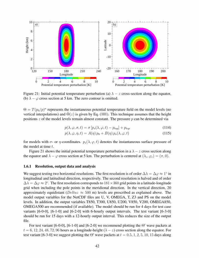
Figure 21: Initial potential temperature perturbation (a) λ − z cross-section along the equator,(b) λ− ϕ cross section at 5 km. The zero contour is omitted.
Θ = T (p0/p)κ represents the instantaneous potential temperature field on the model levels (no
vertical interpolations) and Θ(z) is given by Eq. (101). This technique assumes that the heightpositions z of the model levels remain almost constant. The pressure p can be determined via
p(λ, ϕ, σ, t) = σ [ps(λ, ϕ, t)− ptop] + ptop (114)p(λ, ϕ, η, t) = A(η) p0 +B(η) ps(λ, ϕ, t) (115)
for models with σ- or η-coordinates. ps(λ, ϕ, t) denotes the instantaneous surface pressure ofthe model at time t.
Figure 21 shows the initial potential temperature perturbation in a λ− z cross section alongthe equator and λ− ϕ cross section at 5 km. The perturbation is centered at (λc, ϕc) = (π, 0).
1.6.1 Resolution, output data and analysis
We suggest testing two horizontal resolutions. The first resolution is of order ∆λ = ∆ϕ ≈ 1 inlongitudinal and latitudinal direction, respectively. The second resolution is halved and of order∆λ = ∆ϕ ≈ 2. The first resolution corresponds to 181×360 grid points in a latitude-longitudegrid when including the pole points in the meridional direction. In the vertical direction, 20approximately equidistant (Deltaz ≈ 500 m) levels are prescribed as explained above. Themodel output variables for the NetCDF files are U, V, OMEGA, T, Z3 and PS on the modellevels. In addition, the output variables T850, T300, U850, U200, V850, V200, OMEGA850,OMEGA500 are recommended (if available). The model should be run for 4 days for test casevariants [6-0-0], [6-1-0] and [6-2-0] with 6-hourly output intervals. The test variant [6-3-0]should be run for 15 days with a 12-hourly output interval. This reduces the size of the outputfile.
For test variant [6-0-0], [6-1-0] and [6-2-0] we recommend plotting the Θ′ wave packets att = 6, 12, 24, 48, 72, 96 hours as a longitude-height (λ− z) cross section along the equator. Fortest variant [6-3-0] we suggest plotting the Θ′ wave packets at t = 0.5, 1, 2, 5, 10, 15 days along
42
ϕ = 45. The vertical plotting range is z ∈ [0, 10] km. The horizontal plotting range spans alllongitudes from λ ∈ [0, 360]. Both horizontal resolutions should be compared. The symmetryof the westward and eastward traveling wave packets can be analyzed if no background flow ischosen.
In addition, we recommend plotting latitude-longitude cross sections of the wind anomalies(u-u(t=0)), v and the temperature anomaly (T − T ) at selected levels (850 hPa, 500 hPa, 300hPa) as well as the surface pressure anomaly (ps−ps(t = 0)). The radially outward propagatinggravity wave packets can clearly be seen in all fields at hour 6, 12, 24, 48, 72 and 96. Note thatthe amplitudes of the wave packets are small. The horizontal temperature anomalies lie between0-1 K, the wind variations are on the order of a few m s−1 and the surface pressure anomaliesare a few hPa.
Figures 22 and 23 show snapshots of the potential temperature perturbation Θ′ and surfacepressure anomaly from an NCAR CAM3.5.41 Eulerian simulation for test variant [6-0-0]. Thesnapshots are taken at times 6, 12, 24, 48, 72 and 96 hours from a run with the spectral resolutionT106 (approx. 1 × 1) and 20 vertical levels .
Examples of the potential temperature perturbation from EULT106L20 for test variants [6-1-0] and [6-2-0] are shown in Figs. 24 and 25.
In addition, Figs. 26 and 27 depict the potential temperature perturbation and surface pres-sure anomaly from an NCAR CAM3.5.41 FV simulation for test variant [6-3-0]. The snapshotsare taken at times 0.5, 1, 2, 5, 10, 15 days from a run with the resolution 1× 1 and 20 verticallevels .
2 Typical resolutions, time steps and diffusion coefficientsAll dynamical cores should be run in their operational configurations which includes the typicaldiffusion mechanisms and coefficients, filters, time steps and other tunable parameters. In addi-tion, the runs should utilizes their standard a posteriori fixers like mass or energy fixers if appli-cable. These standard runs serve as a control simulation. All parameters and fixers need to bedocumented to foster model comparisons. In addition, the documentation needs to list the prog-nostic variables, the equation set (e.g. shallow-atmosphere hydrostatic, or shallow-atmospherenonhydrostatic), the horizontal grid staggering, time stepping approach, vertical coordinate andresolution. As an example, we list typical time steps, resolutions and diffusion coefficients forvarious dynamical cores with different numerical approaches in the tables below.
The modeling groups are also invited to test their models in non-operational configurationsthat, for example, use less explicit diffusion. These configurations are often viable for idealizedtest cases as considered here, but might not be applicable in real weather or climate simulations.Therefore, any conclusions need to be carefully drawn and are not necessarily valid for modelswith physics parameterizations.
2.1 Gaussian grids for spectral transform methodsTable 4 lists the horizontal resolutions, time steps and ∇4diffusion coefficients K4 for the spec-tral transform Eulerian dynamical core that is part of NCAR’s CAM3.5 modeling framework.The abbreviation T symbolizes a triangular truncation which is followed by the maximum re-solved wavenumber. The Eulerian dynamical core in vorticity-divergence form is based on
43

Figure 22: Gravity waves at the equator on a non-rotating planet simulated with EULT106L20:Potential temperature perturbation Θ′ at 6, 12, 24, 48, 72 and 96 hours for test scenario 6-0-0.
44
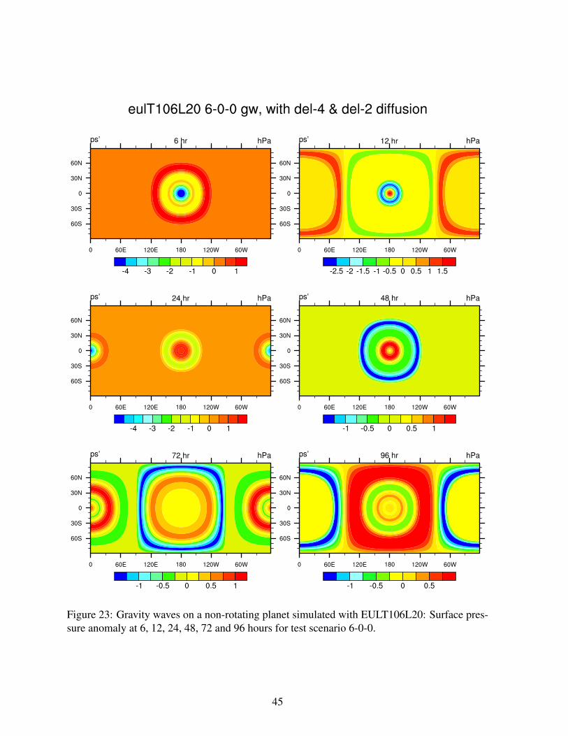
Figure 23: Gravity waves on a non-rotating planet simulated with EULT106L20: Surface pres-sure anomaly at 6, 12, 24, 48, 72 and 96 hours for test scenario 6-0-0.
45
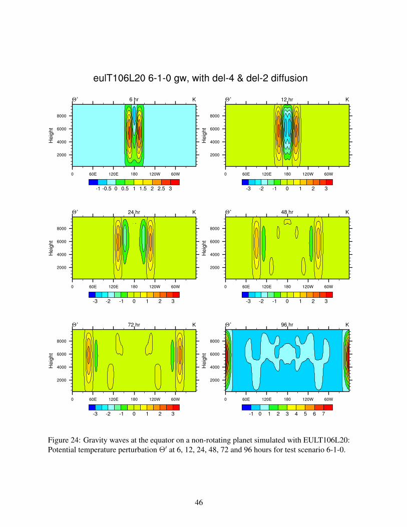
Figure 24: Gravity waves at the equator on a non-rotating planet simulated with EULT106L20:Potential temperature perturbation Θ′ at 6, 12, 24, 48, 72 and 96 hours for test scenario 6-1-0.
46
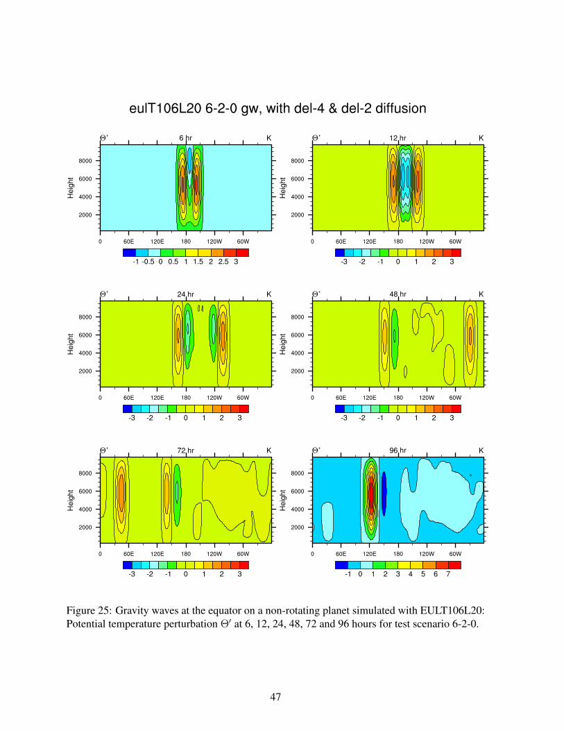
Figure 25: Gravity waves at the equator on a non-rotating planet simulated with EULT106L20:Potential temperature perturbation Θ′ at 6, 12, 24, 48, 72 and 96 hours for test scenario 6-2-0.
47
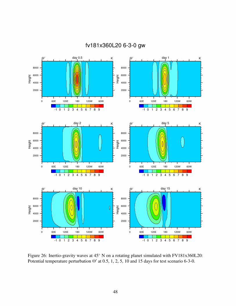
Figure 26: Inertio-gravity waves at 45 N on a rotating planet simulated with FV181x360L20:Potential temperature perturbation Θ′ at 0.5, 1, 2, 5, 10 and 15 days for test scenario 6-3-0.
48
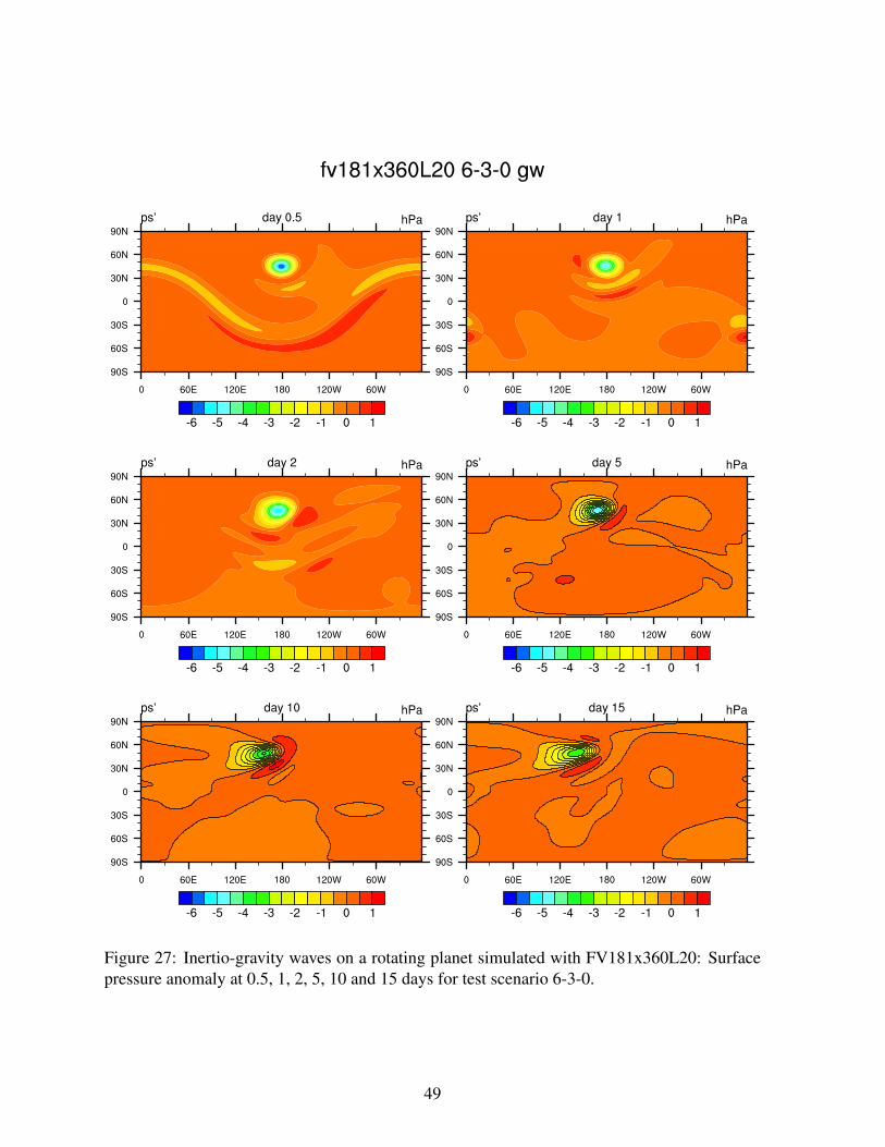
Figure 27: Inertio-gravity waves on a rotating planet simulated with FV181x360L20: Surfacepressure anomaly at 0.5, 1, 2, 5, 10 and 15 days for test scenario 6-3-0.
49
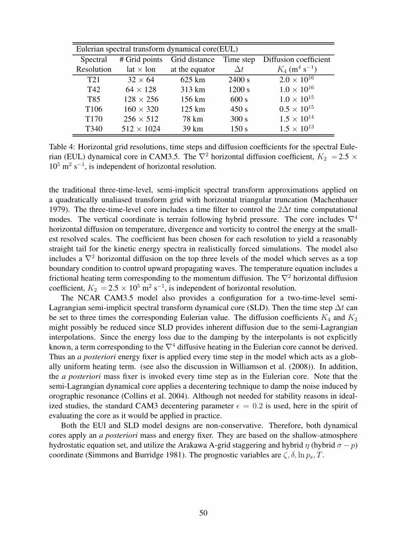
Eulerian spectral transform dynamical core(EUL)Spectral # Grid points Grid distance Time step Diffusion coefficient
Resolution lat × lon at the equator ∆t K4 (m4 s−1)T21 32 × 64 625 km 2400 s 2.0 × 10¹⁶
T42 64 × 128 313 km 1200 s 1.0 × 10¹⁶
T85 128 × 256 156 km 600 s 1.0 × 10¹⁵
T106 160 × 320 125 km 450 s 0.5 × 10¹⁵
T170 256 × 512 78 km 300 s 1.5 × 10¹⁴
T340 512 × 1024 39 km 150 s 1.5 × 10¹³
Table 4: Horizontal grid resolutions, time steps and diffusion coefficients for the spectral Eule-rian (EUL) dynamical core in CAM3.5. The ∇2 horizontal diffusion coefficient, K2 = 2.5 ×10⁵ m2 s−1, is independent of horizontal resolution.
the traditional three-time-level, semi-implicit spectral transform approximations applied ona quadratically unaliased transform grid with horizontal triangular truncation (Machenhauer1979). The three-time-level core includes a time filter to control the 2∆t time computationalmodes. The vertical coordinate is terrain following hybrid pressure. The core includes ∇4
horizontal diffusion on temperature, divergence and vorticity to control the energy at the small-est resolved scales. The coefficient has been chosen for each resolution to yield a reasonablystraight tail for the kinetic energy spectra in realistically forced simulations. The model alsoincludes a ∇2 horizontal diffusion on the top three levels of the model which serves as a topboundary condition to control upward propagating waves. The temperature equation includes africtional heating term corresponding to the momentum diffusion. The ∇2 horizontal diffusioncoefficient, K2 = 2.5 × 10⁵ m2 s−1, is independent of horizontal resolution.
The NCAR CAM3.5 model also provides a configuration for a two-time-level semi-Lagrangian semi-implicit spectral transform dynamical core (SLD). Then the time step ∆t canbe set to three times the corresponding Eulerian value. The diffusion coefficients K4 and K2
might possibly be reduced since SLD provides inherent diffusion due to the semi-Lagrangianinterpolations. Since the energy loss due to the damping by the interpolants is not explicitlyknown, a term corresponding to the∇4 diffusive heating in the Eulerian core cannot be derived.Thus an a posteriori energy fixer is applied every time step in the model which acts as a glob-ally uniform heating term. (see also the discussion in Williamson et al. (2008)). In addition,the a posteriori mass fixer is invoked every time step as in the Eulerian core. Note that thesemi-Lagrangian dynamical core applies a decentering technique to damp the noise induced byorographic resonance (Collins et al. 2004). Although not needed for stability reasons in ideal-ized studies, the standard CAM3 decentering parameter ε = 0.2 is used, here in the spirit ofevaluating the core as it would be applied in practice.
Both the EUl and SLD model designs are non-conservative. Therefore, both dynamicalcores apply an a posteriori mass and energy fixer. They are based on the shallow-atmospherehydrostatic equation set, and utilize the Arakawa A-grid staggering and hybrid η (hybrid σ− p)coordinate (Simmons and Burridge 1981). The prognostic variables are ζ, δ, ln ps, T .
50
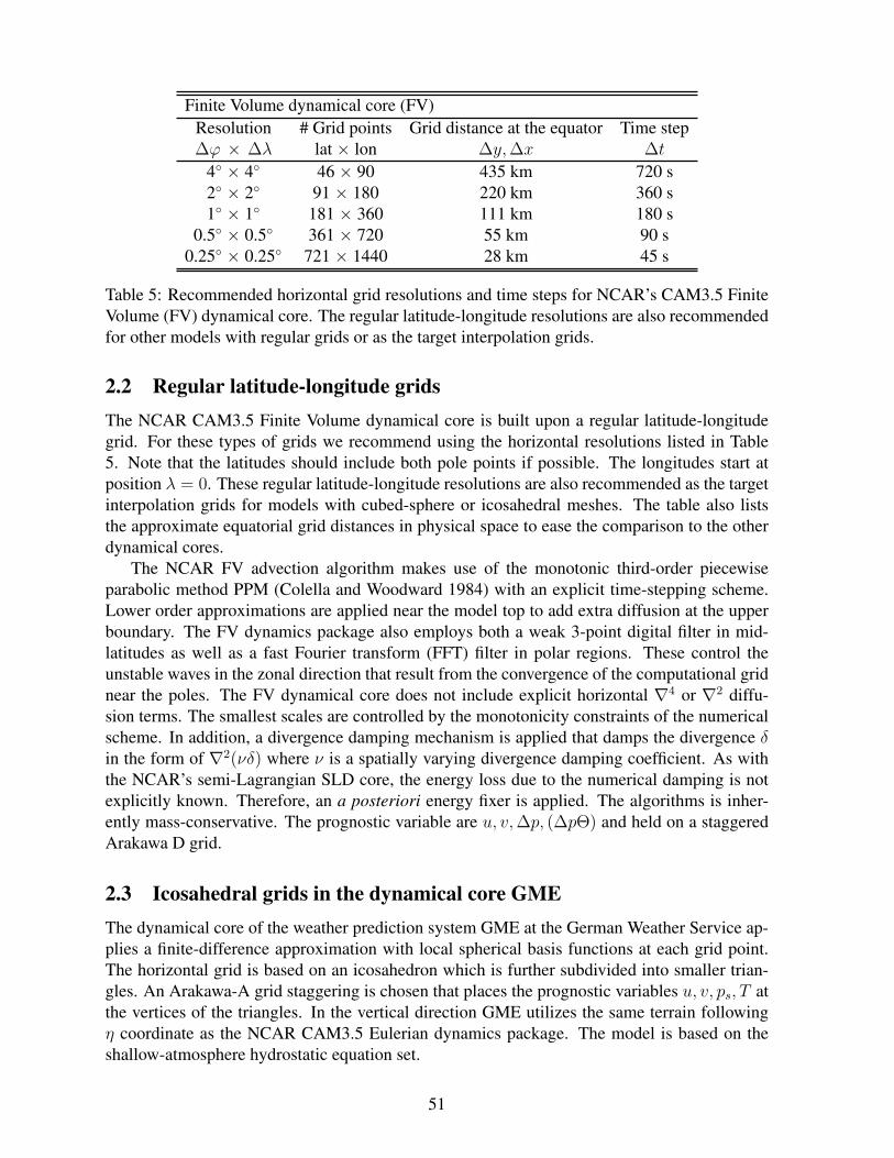
Finite Volume dynamical core (FV)Resolution # Grid points Grid distance at the equator Time step∆ϕ × ∆λ lat × lon ∆y,∆x ∆t
4 × 4 46 × 90 435 km 720 s2 × 2 91 × 180 220 km 360 s1 × 1 181 × 360 111 km 180 s
0.5 × 0.5 361 × 720 55 km 90 s0.25 × 0.25 721 × 1440 28 km 45 s
Table 5: Recommended horizontal grid resolutions and time steps for NCAR’s CAM3.5 FiniteVolume (FV) dynamical core. The regular latitude-longitude resolutions are also recommendedfor other models with regular grids or as the target interpolation grids.
2.2 Regular latitude-longitude gridsThe NCAR CAM3.5 Finite Volume dynamical core is built upon a regular latitude-longitudegrid. For these types of grids we recommend using the horizontal resolutions listed in Table5. Note that the latitudes should include both pole points if possible. The longitudes start atposition λ = 0. These regular latitude-longitude resolutions are also recommended as the targetinterpolation grids for models with cubed-sphere or icosahedral meshes. The table also liststhe approximate equatorial grid distances in physical space to ease the comparison to the otherdynamical cores.
The NCAR FV advection algorithm makes use of the monotonic third-order piecewiseparabolic method PPM (Colella and Woodward 1984) with an explicit time-stepping scheme.Lower order approximations are applied near the model top to add extra diffusion at the upperboundary. The FV dynamics package also employs both a weak 3-point digital filter in mid-latitudes as well as a fast Fourier transform (FFT) filter in polar regions. These control theunstable waves in the zonal direction that result from the convergence of the computational gridnear the poles. The FV dynamical core does not include explicit horizontal ∇4 or ∇2 diffu-sion terms. The smallest scales are controlled by the monotonicity constraints of the numericalscheme. In addition, a divergence damping mechanism is applied that damps the divergence δin the form of ∇2(νδ) where ν is a spatially varying divergence damping coefficient. As withthe NCAR’s semi-Lagrangian SLD core, the energy loss due to the numerical damping is notexplicitly known. Therefore, an a posteriori energy fixer is applied. The algorithms is inher-ently mass-conservative. The prognostic variable are u, v,∆p, (∆pΘ) and held on a staggeredArakawa D grid.
2.3 Icosahedral grids in the dynamical core GMEThe dynamical core of the weather prediction system GME at the German Weather Service ap-plies a finite-difference approximation with local spherical basis functions at each grid point.The horizontal grid is based on an icosahedron which is further subdivided into smaller trian-gles. An Arakawa-A grid staggering is chosen that places the prognostic variables u, v, ps, T atthe vertices of the triangles. In the vertical direction GME utilizes the same terrain followingη coordinate as the NCAR CAM3.5 Eulerian dynamics package. The model is based on theshallow-atmosphere hydrostatic equation set.
51
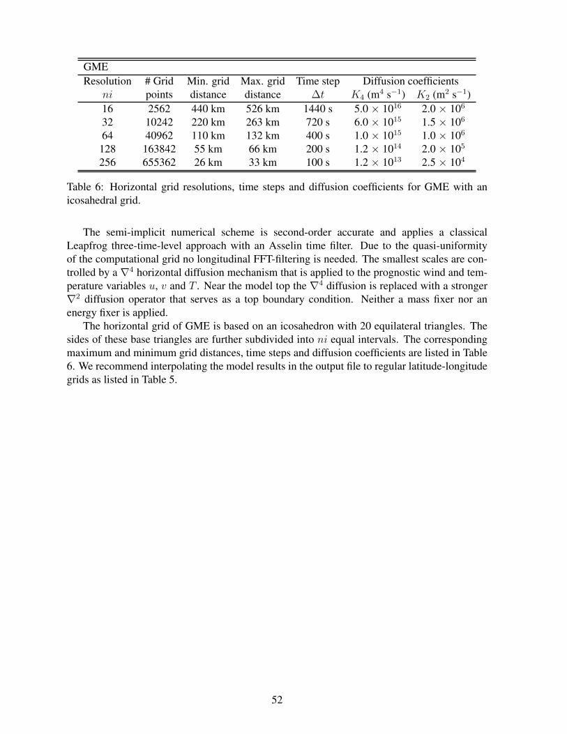
GMEResolution # Grid Min. grid Max. grid Time step Diffusion coefficients
ni points distance distance ∆t K4 (m4 s−1) K2 (m2 s−1)16 2562 440 km 526 km 1440 s 5.0 × 10¹⁶ 2.0 × 10⁶
32 10242 220 km 263 km 720 s 6.0 × 10¹⁵ 1.5 × 10⁶
64 40962 110 km 132 km 400 s 1.0 × 10¹⁵ 1.0 × 10⁶
128 163842 55 km 66 km 200 s 1.2 × 10¹⁴ 2.0 × 10⁵
256 655362 26 km 33 km 100 s 1.2 × 10¹³ 2.5 × 10⁴
Table 6: Horizontal grid resolutions, time steps and diffusion coefficients for GME with anicosahedral grid.
The semi-implicit numerical scheme is second-order accurate and applies a classicalLeapfrog three-time-level approach with an Asselin time filter. Due to the quasi-uniformityof the computational grid no longitudinal FFT-filtering is needed. The smallest scales are con-trolled by a ∇4 horizontal diffusion mechanism that is applied to the prognostic wind and tem-perature variables u, v and T . Near the model top the ∇4 diffusion is replaced with a stronger∇2 diffusion operator that serves as a top boundary condition. Neither a mass fixer nor anenergy fixer is applied.
The horizontal grid of GME is based on an icosahedron with 20 equilateral triangles. Thesides of these base triangles are further subdivided into ni equal intervals. The correspondingmaximum and minimum grid distances, time steps and diffusion coefficients are listed in Table6. We recommend interpolating the model results in the output file to regular latitude-longitudegrids as listed in Table 5.
52
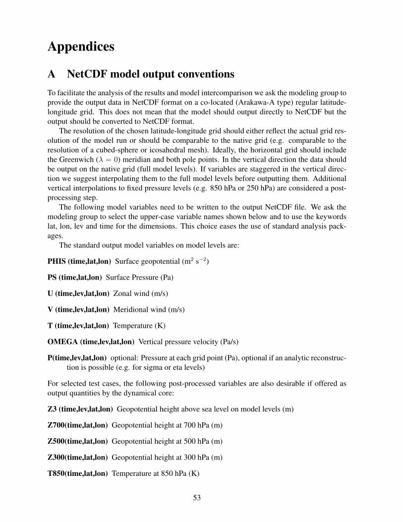
Appendices
A NetCDF model output conventionsTo facilitate the analysis of the results and model intercomparison we ask the modeling group toprovide the output data in NetCDF format on a co-located (Arakawa-A type) regular latitude-longitude grid. This does not mean that the model should output directly to NetCDF but theoutput should be converted to NetCDF format.
The resolution of the chosen latitude-longitude grid should either reflect the actual grid res-olution of the model run or should be comparable to the native grid (e.g. comparable to theresolution of a cubed-sphere or icosahedral mesh). Ideally, the horizontal grid should includethe Greenwich (λ = 0) meridian and both pole points. In the vertical direction the data shouldbe output on the native grid (full model levels). If variables are staggered in the vertical direc-tion we suggest interpolating them to the full model levels before outputting them. Additionalvertical interpolations to fixed pressure levels (e.g. 850 hPa or 250 hPa) are considered a post-processing step.
The following model variables need to be written to the output NetCDF file. We ask themodeling group to select the upper-case variable names shown below and to use the keywordslat, lon, lev and time for the dimensions. This choice eases the use of standard analysis pack-ages.
The standard output model variables on model levels are:
PHIS (time,lat,lon) Surface geopotential (m2 s−2)
PS (time,lat,lon) Surface Pressure (Pa)
U (time,lev,lat,lon) Zonal wind (m/s)
V (time,lev,lat,lon) Meridional wind (m/s)
T (time,lev,lat,lon) Temperature (K)
OMEGA (time,lev,lat,lon) Vertical pressure velocity (Pa/s)
P(time,lev,lat,lon) optional: Pressure at each grid point (Pa), optional if an analytic reconstruc-tion is possible (e.g. for sigma or eta levels)
For selected test cases, the following post-processed variables are also desirable if offered asoutput quantities by the dynamical core:
Z3 (time,lev,lat,lon) Geopotential height above sea level on model levels (m)
Z700(time,lat,lon) Geopotential height at 700 hPa (m)
Z500(time,lat,lon) Geopotential height at 500 hPa (m)
Z300(time,lat,lon) Geopotential height at 300 hPa (m)
T850(time,lat,lon) Temperature at 850 hPa (K)
53
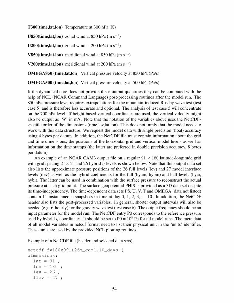
T300(time,lat,lon) Temperature at 300 hPa (K)
U850(time,lat,lon) zonal wind at 850 hPa (m s−1)
U200(time,lat,lon) zonal wind at 200 hPa (m s−1)
V850(time,lat,lon) meridional wind at 850 hPa (m s−1)
V200(time,lat,lon) meridional wind at 200 hPa (m s−1)
OMEGA850 (time,lat,lon) Vertical pressure velocity at 850 hPa (Pa/s)
OMEGA500 (time,lat,lon) Vertical pressure velocity at 500 hPa (Pa/s)
If the dynamical core does not provide these output quantities they can be computed with thehelp of NCL (NCAR Command Language) post-processing routines after the model run. The850 hPa pressure level requires extrapolations for the mountain-induced Rossby wave test (testcase 5) and is therefore less accurate and optional. The analysis of test case 5 will concentrateon the 700 hPa level. If height-based vertical coordinates are used, the vertical velocity mightalso be output as ’W’ in m/s. Note that the notation of the variables above uses the NetCDF-specific order of the dimensions (time,lev,lat,lon). This does not imply that the model needs towork with this data structure. We request the model data with single precision (float) accuracyusing 4 bytes per datum. In addition, the NetCDF file must contain information about the gridand time dimensions, the positions of the horizontal grid and vertical model levels as well asinformation on the time stamps (the latter are preferred in double precision accuracy, 8 bytesper datum).
An example of an NCAR CAM3 output file on a regular 91 × 180 latitude-longitude gridwith grid spacing 2 × 2 and 26 hybrid η-levels is shown below. Note that this output data setalso lists the approximate pressure positions of the 26 full levels (lev) and 27 model interfacelevels (ilev) as well as the hybrid coefficients for the full (hyam, hybm) and half levels (hyai,hybi). The latter can be used in combination with the surface pressure to reconstruct the actualpressure at each grid point. The surface geopotential PHIS is provided as a 3D data set despiteits time-independency. The time-dependent data sets PS, U, V, T and OMEGA (data not listed)contain 11 instantaneous snapshots in time at day 0, 1, 2, 3, ... 10. In addition, the NetCDFheader also lists the post-processed variables. In general, shorter output intervals will also beneeded (e.g. 6-hourly) for the gravity wave test (test case 6). The output frequency should be aninput parameter for the model run. The NetCDF entry P0 corresponds to the reference pressureused by hybrid η coordinates. It should be set to P0 = 105 Pa for all model runs. The meta dataof all model variables in netcdf format need to list their physical unit in the ‘units’ identifier.These units are used by the provided NCL plotting routines.
Example of a NetCDF file (header and selected data sets):
netcdf fv180x091L26g_cam1.10_days dimensions:
lat = 91 ;lon = 180 ;lev = 26 ;ilev = 27 ;
54

time = UNLIMITED ; // (11 currently)variables:
double P0 ;P0:long_name = "reference pressure" ;P0:units = "Pa" ;
double lat(lat) ;lat:long_name = "latitude" ;lat:units = "degrees_north" ;
double lon(lon) ;lon:long_name = "longitude" ;lon:units = "degrees_east" ;
double lev(lev) ;lev:long_name = "hybrid level at midpoints(1000*(A+B))" ;lev:units = "level" ;lev:positive = "down" ;lev:standard_name = "atmosphere_hybrid_sigma_pressure_coordinate" ;lev:formula_terms = "a: hyam b: hybm p0: P0 ps: PS" ;
double ilev(ilev) ;ilev:long_name = "hybrid level at interfaces (1000*(A+B))" ;ilev:units = "level" ;ilev:positive = "down" ;ilev:standard_name = "atmosphere_hybrid_sigma_pressure_coordinate" ;ilev:formula_terms = "a: hyai b: hybi p0: P0 ps: PS" ;
double time(time) ;time:long_name = "time" ;time:units = "days since 0000-01-01 00:00:00" ;
double hyai(ilev) ;hyai:long_name = "hybrid A coefficient at layer interfaces" ;
double hybi(ilev) ;hybi:long_name = "hybrid B coefficient at layer interfaces" ;
double hyam(lev) ;hyam:long_name = "hybrid A coefficient at layer midpoints" ;
double hybm(lev) ;hybm:long_name = "hybrid B coefficient at layer midpoints" ;
float PHIS(lat, lon) ;PHIS:units = mˆ2/sˆ2" ;PHIS:long_name = "Surface geopotential" ;
float PS(time, lat, lon) ;PS:units = "Pa" ;PS:long_name = "Surface pressure" ;
float T(time, lev, lat, lon) ;T:units = "K" ;T:long_name = "Temperature" ;
float U(time, lev, lat, lon) ;U:units = "m/s" ;U:long_name = "Zonal wind" ;
55
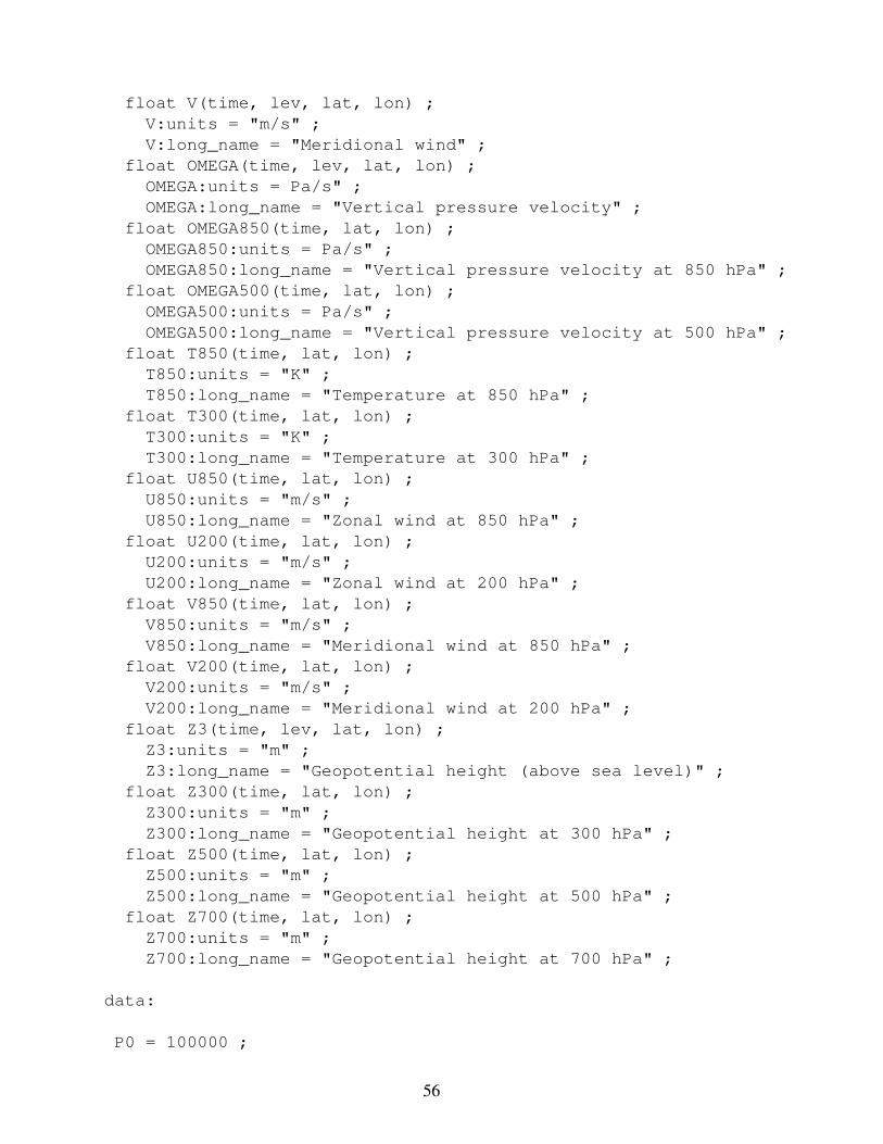
float V(time, lev, lat, lon) ;V:units = "m/s" ;V:long_name = "Meridional wind" ;
float OMEGA(time, lev, lat, lon) ;OMEGA:units = Pa/s" ;OMEGA:long_name = "Vertical pressure velocity" ;
float OMEGA850(time, lat, lon) ;OMEGA850:units = Pa/s" ;OMEGA850:long_name = "Vertical pressure velocity at 850 hPa" ;
float OMEGA500(time, lat, lon) ;OMEGA500:units = Pa/s" ;OMEGA500:long_name = "Vertical pressure velocity at 500 hPa" ;
float T850(time, lat, lon) ;T850:units = "K" ;T850:long_name = "Temperature at 850 hPa" ;
float T300(time, lat, lon) ;T300:units = "K" ;T300:long_name = "Temperature at 300 hPa" ;
float U850(time, lat, lon) ;U850:units = "m/s" ;U850:long_name = "Zonal wind at 850 hPa" ;
float U200(time, lat, lon) ;U200:units = "m/s" ;U200:long_name = "Zonal wind at 200 hPa" ;
float V850(time, lat, lon) ;V850:units = "m/s" ;V850:long_name = "Meridional wind at 850 hPa" ;
float V200(time, lat, lon) ;V200:units = "m/s" ;V200:long_name = "Meridional wind at 200 hPa" ;
float Z3(time, lev, lat, lon) ;Z3:units = "m" ;Z3:long_name = "Geopotential height (above sea level)" ;
float Z300(time, lat, lon) ;Z300:units = "m" ;Z300:long_name = "Geopotential height at 300 hPa" ;
float Z500(time, lat, lon) ;Z500:units = "m" ;Z500:long_name = "Geopotential height at 500 hPa" ;
float Z700(time, lat, lon) ;Z700:units = "m" ;Z700:long_name = "Geopotential height at 700 hPa" ;
data:
P0 = 100000 ;
56
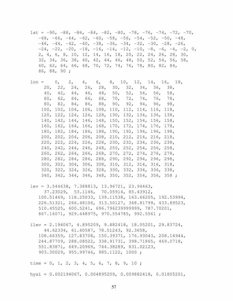
lat = -90, -88, -86, -84, -82, -80, -78, -76, -74, -72, -70,-68, -66, -64, -62, -60, -58, -56, -54, -52, -50, -48,-46, -44, -42, -40, -38, -36, -34, -32, -30, -28, -26,-24, -22, -20, -18, -16, -14, -12, -10, -8, -6, -4, -2, 0,2, 4, 6, 8, 10, 12, 14, 16, 18, 20, 22, 24, 26, 28, 30,32, 34, 36, 38, 40, 42, 44, 46, 48, 50, 52, 54, 56, 58,60, 62, 64, 66, 68, 70, 72, 74, 76, 78, 80, 82, 84,86, 88, 90 ;
lon = 0, 2, 4, 6, 8, 10, 12, 14, 16, 18,20, 22, 24, 26, 28, 30, 32, 34, 36, 38,40, 42, 44, 46, 48, 50, 52, 54, 56, 58,60, 62, 64, 66, 68, 70, 72, 74, 76, 78,80, 82, 84, 86, 88, 90, 92, 94, 96, 98,
100, 102, 104, 106, 108, 110, 112, 114, 116, 118,120, 122, 124, 126, 128, 130, 132, 134, 136, 138,140, 142, 144, 146, 148, 150, 152, 154, 156, 158,160, 162, 164, 166, 168, 170, 172, 174, 176, 178,180, 182, 184, 186, 188, 190, 192, 194, 196, 198,200, 202, 204, 206, 208, 210, 212, 214, 216, 218,220, 222, 224, 226, 228, 230, 232, 234, 236, 238,240, 242, 244, 246, 248, 250, 252, 254, 256, 258,260, 262, 264, 266, 268, 270, 272, 274, 276, 278,280, 282, 284, 286, 288, 290, 292, 294, 296, 298,300, 302, 304, 306, 308, 310, 312, 314, 316, 318,320, 322, 324, 326, 328, 330, 332, 334, 336, 338,340, 342, 344, 346, 348, 350, 352, 354, 356, 358 ;
lev = 3.544638, 7.388813, 13.96721, 23.94463,37.23029, 53.1146, 70.05914, 85.43912,
100.51469, 118.25033, 139.11538, 163.66205, 192.53994,226.51321, 266.48106, 313.50127, 368.81799, 433.89523,510.45525, 600.5241, 696.796239999999, 787.70201,867.16071, 929.648975, 970.554785, 992.5561 ;
ilev = 2.194067, 4.895209, 9.882418, 18.05201, 29.83724,44.62334, 61.60587, 78.51243, 92.3658,
108.66359, 127.83708, 150.39371, 176.93043, 208.14944,244.87709, 288.08522, 338.91731, 398.71865, 469.0718,551.83871, 649.20969, 744.38289, 831.02123,903.30029, 955.99746, 985.1122, 1000 ;
time = 0, 1, 2, 3, 4, 5, 6, 7, 8, 9, 10 ;
hyai = 0.002194067, 0.004895209, 0.009882418, 0.01805201,
57
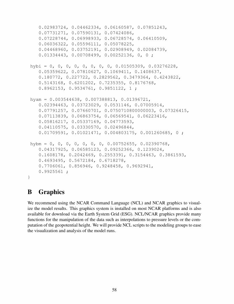
0.02983724, 0.04462334, 0.06160587, 0.07851243,0.07731271, 0.07590131, 0.07424086,0.07228744, 0.06998933, 0.06728574, 0.06410509,0.06036322, 0.05596111, 0.05078225,0.04468960, 0.03752191, 0.02908949, 0.02084739,0.01334443, 0.00708499, 0.00252136, 0, 0 ;
hybi = 0, 0, 0, 0, 0, 0, 0, 0, 0.01505309, 0.03276228,0.05359622, 0.07810627, 0.1069411, 0.1408637,0.180772, 0.227722, 0.2829562, 0.3479364, 0.4243822,0.5143168, 0.6201202, 0.7235355, 0.8176768,0.8962153, 0.9534761, 0.9851122, 1 ;
hyam = 0.003544638, 0.007388813, 0.01396721,0.02394463, 0.03723029, 0.0531146, 0.07005914,0.07791257, 0.07660701, 0.0750710800000003, 0.07326415,0.07113839, 0.06863754, 0.06569541, 0.06223416,0.05816217, 0.05337169, 0.04773593,0.04110575, 0.03330570, 0.02496844,0.01709591, 0.01021471, 0.004803175, 0.001260685, 0 ;
hybm = 0, 0, 0, 0, 0, 0, 0, 0.00752655, 0.02390768,0.04317925, 0.06585123, 0.09252366, 0.1239024,0.1608178, 0.2042469, 0.2553391, 0.3154463, 0.3861593,0.4693495, 0.5672184, 0.6718278,0.7706061, 0.856946, 0.9248458, 0.9692941,0.9925561 ;
B GraphicsWe recommend using the NCAR Command Language (NCL) and NCAR graphics to visual-ize the model results. This graphics system is installed on most NCAR platforms and is alsoavailable for download via the Earth System Grid (ESG). NCL/NCAR graphics provide manyfunctions for the manipulation of the data such as interpolations to pressure levels or the com-putation of the geopotential height. We will provide NCL scripts to the modeling groups to easethe visualization and analysis of the model runs.
58
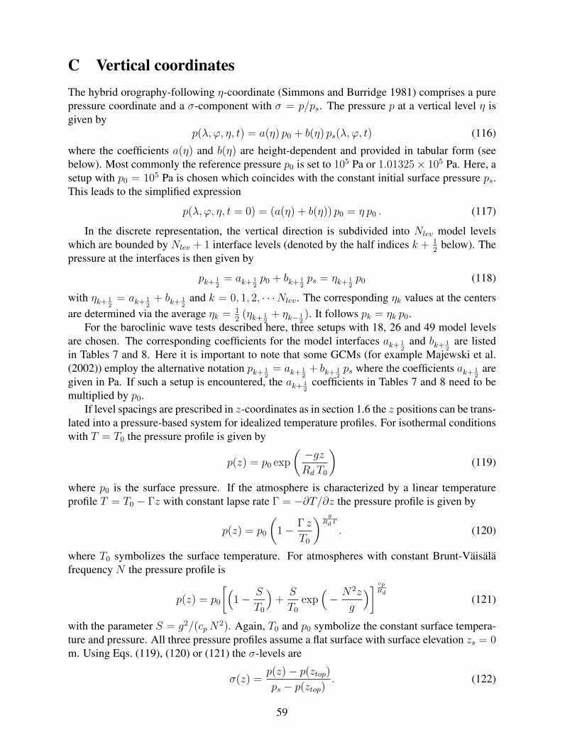
C Vertical coordinatesThe hybrid orography-following η-coordinate (Simmons and Burridge 1981) comprises a purepressure coordinate and a σ-component with σ = p/ps. The pressure p at a vertical level η isgiven by
p(λ, ϕ, η, t) = a(η) p0 + b(η) ps(λ, ϕ, t) (116)
where the coefficients a(η) and b(η) are height-dependent and provided in tabular form (seebelow). Most commonly the reference pressure p0 is set to 105 Pa or 1.01325× 10⁵ Pa. Here, asetup with p0 = 105 Pa is chosen which coincides with the constant initial surface pressure ps.This leads to the simplified expression
p(λ, ϕ, η, t = 0) = (a(η) + b(η)) p0 = η p0 . (117)
In the discrete representation, the vertical direction is subdivided into Nlev model levelswhich are bounded by Nlev + 1 interface levels (denoted by the half indices k + 1
2below). The
pressure at the interfaces is then given by
pk+ 12
= ak+ 12p0 + bk+ 1
2ps = ηk+ 1
2p0 (118)
with ηk+ 12
= ak+ 12
+ bk+ 12
and k = 0, 1, 2, · · ·Nlev. The corresponding ηk values at the centersare determined via the average ηk = 1
2(ηk+ 1
2+ ηk− 1
2). It follows pk = ηk p0.
For the baroclinic wave tests described here, three setups with 18, 26 and 49 model levelsare chosen. The corresponding coefficients for the model interfaces ak+ 1
2and bk+ 1
2are listed
in Tables 7 and 8. Here it is important to note that some GCMs (for example Majewski et al.(2002)) employ the alternative notation pk+ 1
2= ak+ 1
2+ bk+ 1
2ps where the coefficients ak+ 1
2are
given in Pa. If such a setup is encountered, the ak+ 12
coefficients in Tables 7 and 8 need to bemultiplied by p0.
If level spacings are prescribed in z-coordinates as in section 1.6 the z positions can be trans-lated into a pressure-based system for idealized temperature profiles. For isothermal conditionswith T = T0 the pressure profile is given by
p(z) = p0 exp
( −gzRd T0
)(119)
where p0 is the surface pressure. If the atmosphere is characterized by a linear temperatureprofile T = T0 − Γz with constant lapse rate Γ = −∂T/∂z the pressure profile is given by
p(z) = p0
(1− Γ z
T0
) gRd Γ
. (120)
where T0 symbolizes the surface temperature. For atmospheres with constant Brunt-Vaisalafrequency N the pressure profile is
p(z) = p0
[(1− S
T0
)+S
T0
exp(− N2z
g
)] cpRd
(121)
with the parameter S = g2/(cpN2). Again, T0 and p0 symbolize the constant surface tempera-
ture and pressure. All three pressure profiles assume a flat surface with surface elevation zs = 0m. Using Eqs. (119), (120) or (121) the σ-levels are
σ(z) =p(z)− p(ztop)
ps − p(ztop). (122)
59
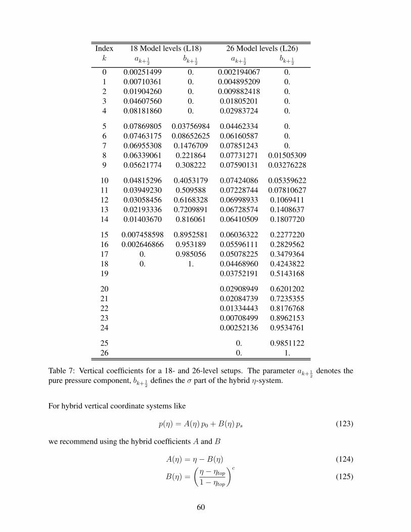
Index 18 Model levels (L18) 26 Model levels (L26)k ak+ 1
2bk+ 1
2ak+ 1
2bk+ 1
2
0 0.00251499 0. 0.002194067 0.1 0.00710361 0. 0.004895209 0.2 0.01904260 0. 0.009882418 0.3 0.04607560 0. 0.01805201 0.4 0.08181860 0. 0.02983724 0.
5 0.07869805 0.03756984 0.04462334 0.6 0.07463175 0.08652625 0.06160587 0.7 0.06955308 0.1476709 0.07851243 0.8 0.06339061 0.221864 0.07731271 0.015053099 0.05621774 0.308222 0.07590131 0.03276228
10 0.04815296 0.4053179 0.07424086 0.0535962211 0.03949230 0.509588 0.07228744 0.0781062712 0.03058456 0.6168328 0.06998933 0.106941113 0.02193336 0.7209891 0.06728574 0.140863714 0.01403670 0.816061 0.06410509 0.1807720
15 0.007458598 0.8952581 0.06036322 0.227722016 0.002646866 0.953189 0.05596111 0.282956217 0. 0.985056 0.05078225 0.347936418 0. 1. 0.04468960 0.424382219 0.03752191 0.5143168
20 0.02908949 0.620120221 0.02084739 0.723535522 0.01334443 0.817676823 0.00708499 0.896215324 0.00252136 0.9534761
25 0. 0.985112226 0. 1.
Table 7: Vertical coefficients for a 18- and 26-level setups. The parameter ak+ 12
denotes thepure pressure component, bk+ 1
2defines the σ part of the hybrid η-system.
For hybrid vertical coordinate systems like
p(η) = A(η) p0 +B(η) ps (123)
we recommend using the hybrid coefficients A and B
A(η) = η −B(η) (124)
B(η) =
(η − ηtop
1− ηtop
)c
(125)
60
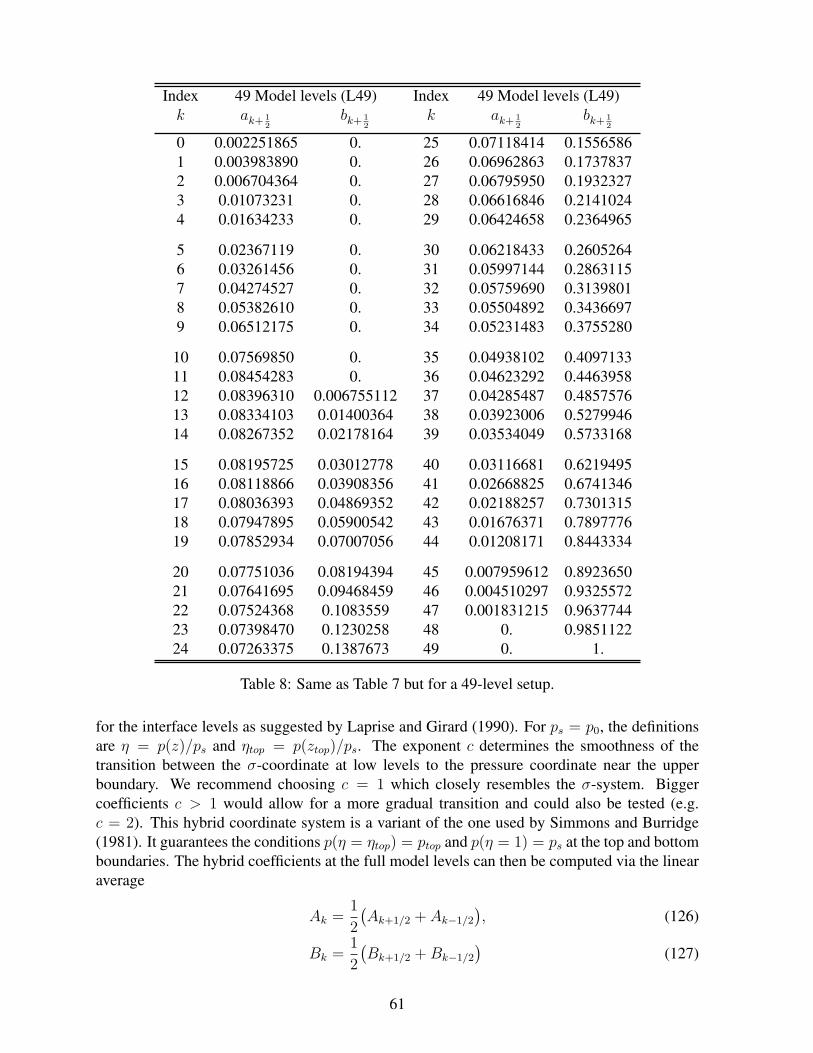
Index 49 Model levels (L49) Index 49 Model levels (L49)k ak+ 1
2bk+ 1
2k ak+ 1
2bk+ 1
2
0 0.002251865 0. 25 0.07118414 0.15565861 0.003983890 0. 26 0.06962863 0.17378372 0.006704364 0. 27 0.06795950 0.19323273 0.01073231 0. 28 0.06616846 0.21410244 0.01634233 0. 29 0.06424658 0.2364965
5 0.02367119 0. 30 0.06218433 0.26052646 0.03261456 0. 31 0.05997144 0.28631157 0.04274527 0. 32 0.05759690 0.31398018 0.05382610 0. 33 0.05504892 0.34366979 0.06512175 0. 34 0.05231483 0.3755280
10 0.07569850 0. 35 0.04938102 0.409713311 0.08454283 0. 36 0.04623292 0.446395812 0.08396310 0.006755112 37 0.04285487 0.485757613 0.08334103 0.01400364 38 0.03923006 0.527994614 0.08267352 0.02178164 39 0.03534049 0.5733168
15 0.08195725 0.03012778 40 0.03116681 0.621949516 0.08118866 0.03908356 41 0.02668825 0.674134617 0.08036393 0.04869352 42 0.02188257 0.730131518 0.07947895 0.05900542 43 0.01676371 0.789777619 0.07852934 0.07007056 44 0.01208171 0.8443334
20 0.07751036 0.08194394 45 0.007959612 0.892365021 0.07641695 0.09468459 46 0.004510297 0.932557222 0.07524368 0.1083559 47 0.001831215 0.963774423 0.07398470 0.1230258 48 0. 0.985112224 0.07263375 0.1387673 49 0. 1.
Table 8: Same as Table 7 but for a 49-level setup.
for the interface levels as suggested by Laprise and Girard (1990). For ps = p0, the definitionsare η = p(z)/ps and ηtop = p(ztop)/ps. The exponent c determines the smoothness of thetransition between the σ-coordinate at low levels to the pressure coordinate near the upperboundary. We recommend choosing c = 1 which closely resembles the σ-system. Biggercoefficients c > 1 would allow for a more gradual transition and could also be tested (e.g.c = 2). This hybrid coordinate system is a variant of the one used by Simmons and Burridge(1981). It guarantees the conditions p(η = ηtop) = ptop and p(η = 1) = ps at the top and bottomboundaries. The hybrid coefficients at the full model levels can then be computed via the linearaverage
Ak =1
2
(Ak+1/2 + Ak−1/2
), (126)
Bk =1
2
(Bk+1/2 +Bk−1/2
)(127)
61
where the index k denotes the discrete full model level which is surrounded by the two inter-face levels shown with half indices. The linear average guarantees that vertical differencingoperations conserve energy. We again note that some models (Majewski et al. 2002) use thealternative definition of Eq. (123)
p(η) = A(η) + B(η) ps. (128)
Then Eq. (124) is represented by A(η) = p0[η −B(η)].
62
D Iterative Method for Dynamical Cores with z- or Θ-BasedVertical Coordinates
In sections 1.1 and 1.2 the initial conditions are shown in closed form for pressure-based verticalcoordinates with η = σ = p/ps. For dynamical cores with z- or Θ-based vertical coordinates aroot-finding technique (Newton’s method) is suggested. It determines the corresponding η-levelfor any given height z or isentropic level Θ with high accuracy. This technique therefore avoidsvertical interpolations of the initial data set. The iterative method is given by
ηn+1 = ηn − F (λ, ϕ, ηn)∂F∂η
(λ, ϕ, ηn)(129)
where the superscript n = 0, 1, 2, 3, . . . indicates the iteration count.For a given z-level the functions F and ∂F/∂η are determined by
F (λ, ϕ, ηn) = −g z + Φ(λ, ϕ, ηn) (130)∂F
∂η(λ, ϕ, ηn) = −Rd
ηnT (λ, ϕ, ηn) (131)
where T and Φ are shown in Eqs. (10) and (11), respectively.If isentropic vertical coordinates with given Θ-levels are utilized the function F is defined
byF (λ, ϕ, ηn) = −Θ + (ηn)−κ T (λ, ϕ, ηn) (132)
with κ = Rd/cp. The specific heat of dry air at constant pressure cp is set to 1004.64 J (kg K)−1.Using Rd = 287.04 J (kg K)−1, κ is identical to 2/7. For ∂F/∂η it follows
∂F
∂η(λ, ϕ, ηn) = G(ηn)− 3π u0
4Rd (ηn)κcos
12 ηn
v
3 π
2u0η
nC sin2 ηnv cos
12 ηn
v− (133)(2C u0 cos
32 ηn
v +DaΩ) (
(1− κ) sin ηnv +
π ηn
4 cos ηnv
(2− 3 sin2 ηnv )
)
with
C =(− 2 sin6 ϕ (cos2 ϕ+
1
3) +
10
63
)(134)
D =(8
5cos3 ϕ (sin2 ϕ+
2
3)− π
4
)(135)
and ηnv = ((ηn − η0)π/2). As before, η0 is set to 0.252 and ηt = 0.2 is the tropopause
level. G symbolizes the vertical derivative of the horizontal-mean potential temperature Θ(η) =η−κT (η). It is given by
G(ηn) = T0
(Rd Γ
g− κ
)(ηn)(
RdΓ
g−κ−1) (for ηs ≥ ηn ≥ ηt) (136)
G(ηn) = T0
(Rd Γ
g− κ
)(ηn)(
RdΓ
g−κ−1) − ∆T
(ηn)(κ+1)(ηt − ηn)4
(κ ηt + ηn(5− κ)
)
(for ηt > ηn) . (137)
63
The starting value η0 = 10−7 is recommended for all Newton iterations following Eq. (129).Then Newton’s method converges for any given height z below zmax = 100 km or any givenpotential temperature Θ below Θmax = 15000 K. Note that the convergence is only achievedif η0 is greater than zero and physically lies above the uppermost model level. If models withhigher model tops are used, η0 needs to be decreased. We have observed that this iterativetechnique converges within a maximum of 25 iterations. Then the absolute error |η − ηn|is decreased to machine precision (10−14 for double-precision arithmetics). Most often, theconvergence is already achieved with fewer iterations. The resulting η-level can now be usedfor the computation of the analytic initial conditions at the location (λ, ϕ, η).
64
E Transformations for rotated coordinatesThe rotation of the coordinates, together with their inverse relations, has been described inNair and Jablonowski (2008) and Staniforth and White (2007). Here, we partly cite from thereference by Staniforth and White (2007) and add the details for the initial conditions of thesteady-state and baroclinic wave test cases. Note that the trigonometric functions as outlinedbelow might suffer from precision problems due to the nesting and the application of inversetrigonometric functions. Therefore, a slightly different but highly precise method has beenimplemented in the Fortran example code made available to the modeling groups on the NCARWiki web page
https://wiki.ucar.edu/display/dycores/Test+cases
The following steps illustrate the basic principle behind the rotations. Let the North poleof a rotated coordinate system be located at the point (λp, ϕp) of the unrotated geographicalcoordinate system. This is schematically shown in Fig. 28 (Nair and Jablonowski 2008). Let usassume λp = 0 for the calculations here. For a flow orientation angle α the North Pole positionis given by (λp, π/2−α). From Ritchie (1987), the following relations hold between the rotated(λ′, ϕ′) and unrotated (λ, ϕ) coordinate systems:
sinϕ′ = sinϕ sinϕp + cosϕ cosϕp cos(λ− λp), (138)sinϕ = sinϕ′ sinϕp − cosϕ′ cosϕp cosλ′, (139)
cosϕ sin(λ− λp) = cosϕ′ sinλ′. (140)
For the steady-state conditions of section 1.1, expressed in the unrotated (λ, ϕ) coordinate sys-tem, the horizontal wind components at each vertical level satisfy
u(ϕ) = a cosϕDλ
Dt, v = a
Dϕ
Dt= 0, (141)
whilst the wind components in the rotated system satisfy
u′(λ′, ϕ′) = a cosϕ′Dλ′
Dt, v′(λ′, ϕ′) = a
Dϕ′
Dt. (142)
Differentiating Eq. (138) with respect to time and using Eqs. (141) and (142) gives
v′(λ′, ϕ′) cosϕ′ = − cosϕp sin(λ− λp)u(ϕ). (143)
Differentiating Eqs. (139) and (140) with respect to time and manipulating the resulting equa-tions using (140) - (143) then yields
u′(λ′, ϕ′) =[cosλ′ cos(λ− λp) + sinϕp sinλ′ sin(λ− λp)
]u(ϕ) . (144)
Suppose now that the initial conditions in section 1.1 are to be expressed in the (λ′, ϕ′) coor-dinate system, whose North Pole is located at the point (λp, ϕp) of the unrotated geographicalcoordinate system (λ, ϕ). The steps for obtaining the initial conditions at the meshpoints (λ′, ϕ′)of the rotated system are:
65
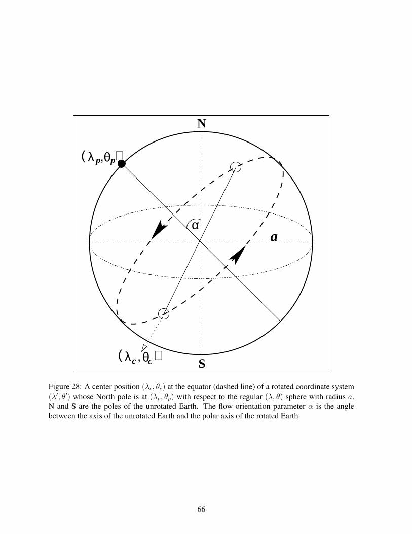
,
( ,p
S
N
λ θp)
a
( λ θc )c
α
Figure 28: A center position (λc, θc) at the equator (dashed line) of a rotated coordinate system(λ′, θ′) whose North pole is at (λp, θp) with respect to the regular (λ, θ) sphere with radius a.N and S are the poles of the unrotated Earth. The flow orientation parameter α is the anglebetween the axis of the unrotated Earth and the polar axis of the rotated Earth.
66
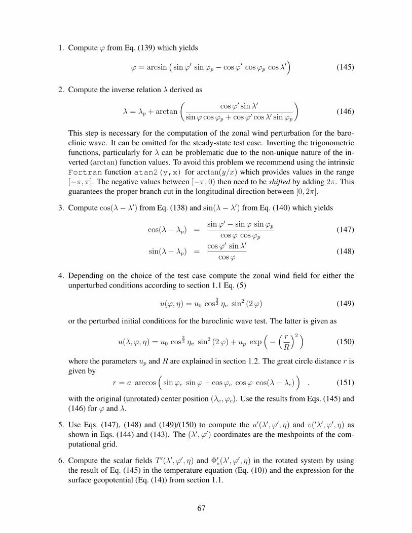
1. Compute ϕ from Eq. (139) which yields
ϕ = arcsin(sinϕ′ sinϕp − cosϕ′ cosϕp cosλ′
)(145)
2. Compute the inverse relation λ derived as
λ = λp + arctan
(cosϕ′ sinλ′
sinϕ cosϕp + cosϕ′ cosλ′ sinϕp
)(146)
This step is necessary for the computation of the zonal wind perturbation for the baro-clinic wave. It can be omitted for the steady-state test case. Inverting the trigonometricfunctions, particularly for λ can be problematic due to the non-unique nature of the in-verted (arctan) function values. To avoid this problem we recommend using the intrinsicFortran function atan2(y,x) for arctan(y/x) which provides values in the range[−π, π]. The negative values between [−π, 0) then need to be shifted by adding 2π. Thisguarantees the proper branch cut in the longitudinal direction between [0, 2π].
3. Compute cos(λ− λ′) from Eq. (138) and sin(λ− λ′) from Eq. (140) which yields
cos(λ− λp) =sinϕ′ − sinϕ sinϕp
cosϕ cosϕp
(147)
sin(λ− λp) =cosϕ′ sinλ′
cosϕ(148)
4. Depending on the choice of the test case compute the zonal wind field for either theunperturbed conditions according to section 1.1 Eq. (5)
u(ϕ, η) = u0 cos32 ηv sin2 (2ϕ) (149)
or the perturbed initial conditions for the baroclinic wave test. The latter is given as
u(λ, ϕ, η) = u0 cos32 ηv sin2 (2ϕ) + up exp
(−
( rR
)2 )(150)
where the parameters up and R are explained in section 1.2. The great circle distance r isgiven by
r = a arccos(
sinϕc sinϕ+ cosϕc cosϕ cos(λ− λc))
. (151)
with the original (unrotated) center position (λc, ϕc). Use the results from Eqs. (145) and(146) for ϕ and λ.
5. Use Eqs. (147), (148) and (149)/(150) to compute the u′(λ′, ϕ′, η) and v(′λ′, ϕ′, η) asshown in Eqs. (144) and (143). The (λ′, ϕ′) coordinates are the meshpoints of the com-putational grid.
6. Compute the scalar fields T ′(λ′, ϕ′, η) and Φ′s(λ
′, ϕ′, η) in the rotated system by usingthe result of Eq. (145) in the temperature equation (Eq. (10)) and the expression for thesurface geopotential (Eq. (14)) from section 1.1.
67
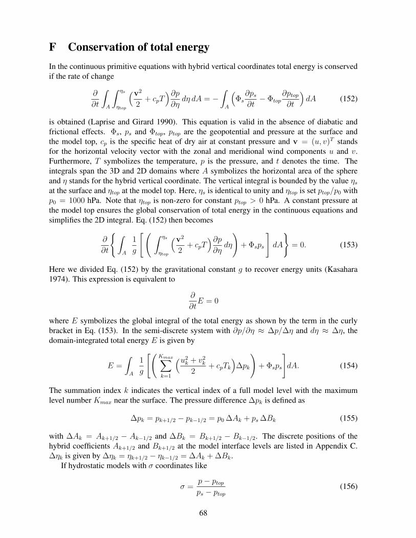
F Conservation of total energyIn the continuous primitive equations with hybrid vertical coordinates total energy is conservedif the rate of change
∂
∂t
∫
A
∫ ηs
ηtop
(v2
2+ cpT
)∂p∂η
dη dA = −∫
A
(Φs∂ps
∂t− Φtop
∂ptop
∂t
)dA (152)
is obtained (Laprise and Girard 1990). This equation is valid in the absence of diabatic andfrictional effects. Φs, ps and Φtop, ptop are the geopotential and pressure at the surface andthe model top, cp is the specific heat of dry air at constant pressure and v = (u, v)T standsfor the horizontal velocity vector with the zonal and meridional wind components u and v.Furthermore, T symbolizes the temperature, p is the pressure, and t denotes the time. Theintegrals span the 3D and 2D domains where A symbolizes the horizontal area of the sphereand η stands for the hybrid vertical coordinate. The vertical integral is bounded by the value ηs
at the surface and ηtop at the model top. Here, ηs is identical to unity and ηtop is set ptop/p0 withp0 = 1000 hPa. Note that ηtop is non-zero for constant ptop > 0 hPa. A constant pressure atthe model top ensures the global conservation of total energy in the continuous equations andsimplifies the 2D integral. Eq. (152) then becomes
∂
∂t
∫
A
1
g
[( ∫ ηs
ηtop
(v2
2+ cpT
)∂p∂η
dη
)+ Φsps
]dA
= 0. (153)
Here we divided Eq. (152) by the gravitational constant g to recover energy units (Kasahara1974). This expression is equivalent to
∂
∂tE = 0
where E symbolizes the global integral of the total energy as shown by the term in the curlybracket in Eq. (153). In the semi-discrete system with ∂p/∂η ≈ ∆p/∆η and dη ≈ ∆η, thedomain-integrated total energy E is given by
E =
∫
A
1
g
[(Kmax∑
k=1
(u2k + v2
k
2+ cpTk
)∆pk
)+ Φsps
]dA. (154)
The summation index k indicates the vertical index of a full model level with the maximumlevel number Kmax near the surface. The pressure difference ∆pk is defined as
∆pk = pk+1/2 − pk−1/2 = p0 ∆Ak + ps ∆Bk (155)
with ∆Ak = Ak+1/2 − Ak−1/2 and ∆Bk = Bk+1/2 − Bk−1/2. The discrete positions of thehybrid coefficients Ak+1/2 and Bk+1/2 at the model interface levels are listed in Appendix C.∆ηk is given by ∆ηk = ηk+1/2 − ηk−1/2 = ∆Ak + ∆Bk.
If hydrostatic models with σ coordinates like
σ =p− ptop
ps − ptop
(156)
68
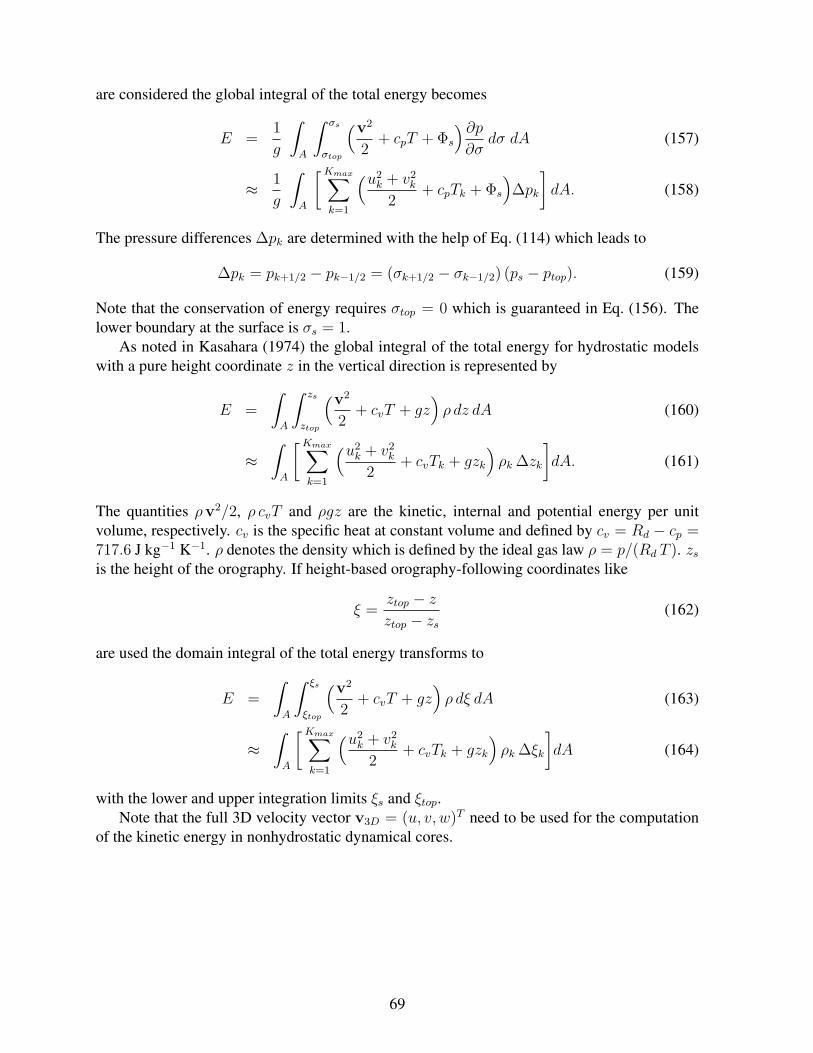
are considered the global integral of the total energy becomes
E =1
g
∫
A
∫ σs
σtop
(v2
2+ cpT + Φs
)∂p∂σ
dσ dA (157)
≈ 1
g
∫
A
[ Kmax∑
k=1
(u2k + v2
k
2+ cpTk + Φs
)∆pk
]dA. (158)
The pressure differences ∆pk are determined with the help of Eq. (114) which leads to
∆pk = pk+1/2 − pk−1/2 = (σk+1/2 − σk−1/2) (ps − ptop). (159)
Note that the conservation of energy requires σtop = 0 which is guaranteed in Eq. (156). Thelower boundary at the surface is σs = 1.
As noted in Kasahara (1974) the global integral of the total energy for hydrostatic modelswith a pure height coordinate z in the vertical direction is represented by
E =
∫
A
∫ zs
ztop
(v2
2+ cvT + gz
)ρ dz dA (160)
≈∫
A
[ Kmax∑
k=1
(u2k + v2
k
2+ cvTk + gzk
)ρk ∆zk
]dA. (161)
The quantities ρv2/2, ρ cvT and ρgz are the kinetic, internal and potential energy per unitvolume, respectively. cv is the specific heat at constant volume and defined by cv = Rd − cp =717.6 J kg−1 K−1. ρ denotes the density which is defined by the ideal gas law ρ = p/(Rd T ). zs
is the height of the orography. If height-based orography-following coordinates like
ξ =ztop − z
ztop − zs
(162)
are used the domain integral of the total energy transforms to
E =
∫
A
∫ ξs
ξtop
(v2
2+ cvT + gz
)ρ dξ dA (163)
≈∫
A
[ Kmax∑
k=1
(u2k + v2
k
2+ cvTk + gzk
)ρk ∆ξk
]dA (164)
with the lower and upper integration limits ξs and ξtop.Note that the full 3D velocity vector v3D = (u, v, w)T need to be used for the computation
of the kinetic energy in nonhydrostatic dynamical cores.
69

G Constants and symbolsPhysical constants and model coordinates
a mean radius of the Earth a = 6.371229× 10⁶ mg gravitational acceleration g = 9.80616 m s−2
Ω Earth’s angular velocity Ω = 2π/sidereal day Ω = 7.29211 ∗ 10−5 s−1
length of a sidereal day 86164 sf Coriolis parameter f = 2Ω sinϕRd ideal gas constant for dry air R = 287.04 J kg−1 K−1
cp specific heat at constant pressure cp = 1004.64 J kg−1 K−1
cv specific heat at constant volume cv = Rd − cp cv = 717.6 J kg−1 K−1
κ κ = Rd/cp = 2/7π π = 3.141592654λ longitude λ ∈ [0, 2π]ϕ latitude ϕ ∈ [−π/2, π/2]η hybrid level η ∈ [0, 1]σ sigma level σ ∈ [0, 1]t timeA(η) hybrid coefficients for η coordinate, also Ak
B(η) hybrid coefficients for η coordinate, also Bk
Symbols and parameters
u zonal wind (unrotated)v meridional wind (unrotated)uperturb perturbation of the zonal windu′ rotated zonal windv′ rotated meridional windω vertical pressure velocity ω = p = dp/dtη vertical velocity in η coordinates η = dη/dtσ vertical velocity in σ coordinates σ = dσ/dtq1− q6 tracer distributionsp pressureρ density ρ = p/(RdT )ps surface pressureT temperatureT horizontal mean temperatureΘ potential temperature Θ = T (1000 hPa
p)κ
Θ′ potential temperature perturbationΘ horizontal mean potential temperature∆Θ potential temperature perturbation amplitude ∆Θ = 10 KΦ geopotentialΦ′ geopotential perturbationΦ horizontal mean geopotentialΦs surface geopotential Φs = gzs
ζ relative vorticity
70
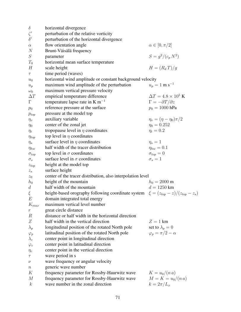
δ horizontal divergenceζ ′ perturbation of the relative vorticityδ′ perturbation of the horizontal divergenceα flow orientation angle α ∈ [0, π/2]N Brunt-Vaisala frequencyS parameter S = g2/(cpN
2)T0 horizontal mean surface temperatureH scale height H = (Rd T )/gτ time period (waves)u0 horizontal wind amplitude or constant background velocityup maximum wind amplitude of the perturbation up = 1 m s−1
ω0 maximum vertical pressure velocity∆T empirical temperature difference ∆T = 4.8× 10⁵ KΓ temperature lapse rate in K m−1 Γ = −∂T/∂zp0 reference pressure at the surface p0 = 1000 hPaptop pressure at the model topηv auxiliary variable ηv = (η − η0)π/2η0 center of the zonal jet η0 = 0.252ηt tropopause level in η coordinates ηt = 0.2ηtop top level in η coordinatesηs surface level in η coordinates ηs = 1ηhw half width of the tracer distribution ηhw = 0.1σtop top level in σ coordinates σtop = 0σs surface level in σ coordinates σs = 1ztop height at the model topzs surface heightz0 center of the tracer distribution, also interpolation levelh0 height of the mountain h0 = 2000 md half width of the mountain d = 1250 kmξ height-based orography following coordinate system ξ = (ztop − z)/(ztop − zs)E domain integrated total energyKmax maximum vertical level numberr great circle distanceR distance or half width in the horizontal directionZ half width in the vertical direction Z = 1 kmλp longitudinal position of the rotated North pole set to λp = 0ϕp latitudinal position of the rotated North pole ϕp = π/2− αλc center point in longitudinal directionϕc center point in latitudinal directionηc center point in the vertical directionτ wave period in sν wave frequency or angular velocityn generic wave numberK frequency parameter for Rossby-Haurwitz wave K = u0/(n a)M frequency parameter for Rossby-Haurwitz wave M = K = u0/(n a)k wave number in the zonal direction k = 2π/Lx
71

l wave number in the meridional direction l = 2π/Ly
m wave number in the vertical direction m = 2π/Lz
cx gravity wave phase speed in the zonal directionLx wave length in zonal directionLy wave length in meridional directionLz wave length in the vertical direction
Key symbols for output quantities
U zonal wind, unstaggeredV meridional wind, unstaggeredOMEGA vertical pressure velocityT temperaturePS surface pressurePHIS surface geopotentialZ3 geopotential heightZ700 geopotential height at 700 hPaZ500 geopotential height at 500 hPaZ300 geopotential height at 300 hPaT850 temperature at 850 hPaT300 temperature at 300 hPaU850 zonal wind at 850 hPaU200 zonal wind at 200 hPaV850 zonal wind at 850 hPaV200 zonal wind at 200 hPaOMEGA850 vertical pressure velocity at 850 hPaOMEGA500 vertical pressure velocity at 500 hPa
72
ReferencesColella, P. and P. R. Woodward, 1984: The Piecewise Parabolic Method (PPM) for gas-
dynamical simulations. J. Comput. Phys., 54, 174–201.
Collins, W. D., P. J. Rasch, B. A. Boville, J. J. Hack, J. R. McCaa, D. L. Williamson, B. P.Briegleb, C. M. Bitz, S.-J. Lin, M. Zhang, and Y. Dai, 2006: The formulation and atmosphericsimulation of the Community Atmosphere Model: CAM3. J. Climate, 19, 2144–2161.
Collins, W. D., P. J. Rasch, B. A. Boville, J. J. Hack, J. R. McCaa, D. L. Williamson, J. T. Kiehl,B. Briegleb, C. Bitz, S.-J. Lin, M. Zhang, and Y. Dai, 2004: Description of the NCAR Com-munity Atmosphere Model (CAM3.0). NCAR Tech. Note NCAR/TN-464+STR, NationalCenter for Atmospheric Research, Boulder, Colorado, 226 pp.
Giraldo, F. X. and T. E. Rosmond, 2004: A scalable Spectral Element Eulerian AtmosphericModel (SEE-AM) for NWP: Dynamical core tests. Mon. Wea. Rev., 132, 133–153.
Haurwitz, B., 1940: The motion of atmospheric disturbances on the spherical earth. J. Mar.Res., 3, 254–267.
Jablonowski, C., 2004: Adaptive Grids in Weather and Climate Modeling. Ph.D. dissertation,University of Michigan, Ann Arbor, MI, Department of Atmospheric, Oceanic and SpaceSciences, 292 pp.
Jablonowski, C. and D. L. Williamson, 2006a: A baroclinic instability test case for atmosphericmodel dynamical cores. Quart. J. Roy. Meteor. Soc., 132, 2943–2975.
— 2006b: A baroclinic wave test case for dynamical cores of General Circulation Models:Model intercomparisons. NCAR Tech. Note NCAR/TN-469+STR, National Center for At-mospheric Research, Boulder, Colorado, 89 pp.
Kasahara, A., 1974: Various vertical coordinate systems used for numerical weather prediction.Mon. Wea. Rev., 102, 509–522.
Laprise, R. and C. Girard, 1990: A spectral General Circulation Model using the piecewise-constant finite-element representation on a hybrid vertical coordinate system. J. Climate, 3,32–52.
Lin, S.-J., 2004: A “vertically Lagrangian” finite-volume dynamical core for global models.Mon. Wea. Rev., 132, 2293–2307.
Machenhauer, B., 1979: The spectral method. Numerical Methods Used in Atmospheric Mod-els, A. Kasahara, ed., GARP Publications Series No 17, WMO and ICSU, Geneva, volume 2,121–275.
Majewski, D., D. Liermann, P. Prohl, B. Ritter, M. Buchhold, T. Hanisch, G. Paul, W. Wergen,and J. Baumgardner, 2002: The operational global icosahedral-hexagonal gridpoint modelGME: Description and high-resolution tests. Mon. Wea. Rev., 130, 319–338.
73
Monaco, A. V. and R. T. Williams, 1975: An atmospheric global prediction model using amodified Arakawa differencing scheme. Technical report, Dept. of Meteorology, Naval Post-graduate School, Monterey, CA, NPS-51WU75041, 86pp.
Nair, R. D. and C. Jablonowski, 2008: Moving vortices on the sphere: A test case for horizontaladvection problems. Mon. Wea. Rev., 136, 699–711.
Phillips, N. A., 1957: A coordinate system having some special advantages for numerical fore-casting. J. Meteor., 14, 184–185.
— 1959: Numerical integration of the primitive equations on the hemisphere. Mon. Wea. Rev.,87, 333–345.
Ritchie, H., 1987: Semi-Lagrangian advection on a Gaussian grid. Mon. Wea. Rev., 115, 608–619.
Simmons, A. J. and D. M. Burridge, 1981: An energy and angular-momentum conservingvertical finite-difference scheme and hybrid vertical coordinates. Mon. Wea. Rev., 109, 758–766.
Simmons, A. J. and B. J. Hoskins, 1977: Baroclinic instability on the sphere: Solutions with amore realistic tropopause. J. Atmos. Sci., 34, 581–588.
— 1979: The downstream and upstream development of unstable baroclinic waves. J. Atmos.Sci., 36, 1239–1254.
Staniforth, A. and A. A. White, 2007: Some exact solutions of geophysical fluid dynamicsequations for testing models in spherical and plane geometry. Quart. J. Roy. Meteor. Soc.,133, 1605–1614.
Tomita, H. and M. Sato, 2004: A new dynamical framework of nonhydrostatic global modelusing the icosahedral grid. Fluid Dyn. Res., 34, 357–400.
U.S. Standard Atmosphere, 1976: U.S. Government Printing Office, Washington D.C.
Wan, H., 2008: University of Hamburg and Max-Planck Institute for Meteorology, Hamburg.Ph.D. thesis, to be submitted.
Williamson, D. L., J. B. Drake, J. J. Hack, R. Jakob, and P. N. Swarztrauber, 1992: A standardtest set for numerical approximations to the shallow water equations in spherical geometry.J. Comput. Phys., 102, 211–224.
Williamson, D. L., J. Olson, and C. Jablonowski, 2008: Two dynamical core formulationflaws exposed by a baroclinic instability test case. Mon. Wea. Rev., in review, available athttp://www-personal.umich.edu/cjablono/MWR Williamson et al 2008.pdf.
74