global factors in the term structure of interest rates · explain term structure dynamics in the...

Global Factors in the Term Structureof Interest Rates∗

Mirko Abbritti,a Salvatore Dell’Erba,b Antonio Moreno,a

and Sergio Solab

aUniversity of NavarrabInternational Monetary Fund

This paper introduces unspanned global factors within aFAVAR framework in a flexible reduced-form affine term struc-ture model. We apply our method to a panel of internationalyield curves and show that global factors account for more than80 percent of term premiums in advanced economies. In partic-ular, they tend to explain long-term dynamics in yield curves,as opposed to domestic factors which are instead more relevantfor short-run movements. We uncover a key role for the thirdprincipal component of the global term structure in shapingrisk-neutral rates and term premium dynamics, especially inthe post-2007 period.

JEL Codes: C32, E43, F41, G12.

1. Introduction

Why are there shifts in yield curves across countries? What makesa long-term bond riskier than a short-term bond? What are the ele-ments that determine the variation over time of the “price of risk”?These questions lie at the heart of many monetary policy discussions

∗This paper has been presented at the Federal Reserve Bank of San Francisco,the IMF, the CEA 2013 (Montreal), CEU (Elche), the 2016 International Asso-ciation for Applied Econometrics (Milan), and the 2016 Asset Pricing Workshopin York (United Kingdom). We especially thank an anonymous referee, AntonioDıez de los Rıos, Angel Leon, Sergio Mayordomo, Gonzalo Rubio, Glenn Rude-busch, and Tommaso Trani for useful comments and suggestions. We thank theSpanish Government for financial support (research project ECO 2015-68815-P).The views expressed are those of the authors and do not necessarily representthe views of the IMF and its Executive Board. Corresponding author: AntonioMoreno, Edificio Amigos Campus Universitario, 31009 Pamplona, Spain. E-mail:[email protected]; Tel.: 34 948 425600, ext. 802330.

301

302 International Journal of Central Banking March 2018

held by policymakers, academics, and bond market participants.Time variation in term premiums can in fact greatly complicate thetask of extracting monetary policy expectations from interest rates.Recent empirical studies have undertaken the difficult task of esti-mating term premiums from the yield curves of bond markets andhave reached considerable success (Bauer, Rudebusch, and Wu 2012,2014). This development was made possible by a new class of macro-finance models which, by replicating the dynamics of the entire yieldcurves, can provide accurate measures of the time-varying risk pre-miums on long-term bonds (Wright 2011, Abbritti et al. 2016). Asa result, researchers have used them to back out this risk compo-nent associated with long-term bond prices (Wright 2011; Bauer,Rudebusch, and Wu 2012, 2014, among others).

However, the effects of global forces on the dynamics of inter-est rates have been relatively less studied. Yet, there are compellingreasons to assert that global shocks affect cross-country governmentyield curves. The recent credit crisis, for instance, shows that macro-finance shocks can be crucially transmitted internationally. As a con-sequence of financial integration, a sizable amount of domestic gov-ernment debt is held by foreigners in global capital markets. Thus,positions on foreign bonds are naturally affected by home macro-finance conditions, and vice versa. Despite these important stylizedfacts, studies on the term structure of interest rates tend to pay verylittle attention to international spillovers in yield curves. This papertakes up this challenge and investigates the role of global factors inthe yield curves of several industrialized countries.

We introduce a role for global factors by modeling the law ofmotion for the yield curves as a factor-augmented vector autoregres-sion (FAVAR) similar to Bernanke, Boivin, and Eliasz (2005), Stockand Watson (2005), and Moench (2008).1 In our model, the tradi-tional determinants of the yield curves—level, slope, and curvature—are accompanied by a set of three global factors, extracted asprincipal components from the global term structure. Our samplecovers the yield curves of eight economies: Canada, United King-dom, Japan, Germany, Australia, New Zealand, Switzerland, and

1While traditional FAVAR models are often used on a large cross-sectionof macro variables, we adopt the same estimation technique and apply it to across-section of bond yields.

Vol. 14 No. 2 Global Factors in the Term Structure of Interest Rates 303

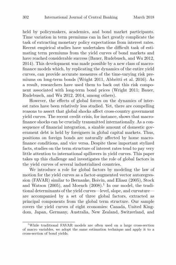
Figure 1. National Yield Curves—First Three Factors

Notes: This figure shows the “level,” “slope,” and “curvature” factors for all thecountries in our sample. Level, slope, and curvature are computed as the first,second, and third principal components extracted from the cross-section of theyields of each country.

the United States. Figure 1 plots the first three principal compo-nents across countries using zero-coupon yields for each country(from three-month to ten-year yields). If co-movement across yieldcurves is a dominant feature, we should then be able to gauge it bylooking at the behavior of these three factors in different countries.The first factor indeed displays strong co-movement across coun-tries. In all cases it has a strong downward trend, and the correlationcoefficient among these series ranges from 0.77 to 0.99. The secondand third factors also display significantly positive cross-correlations,albeit lower, and these correlations become stronger starting around2000. The strong co-movements across the level, slope, and curva-ture factors of the different countries point towards the existence ofglobal forces which may have a strong influence on the shape and


evolution of the yield curves in general, and term premiums in par-ticular. What are they, and how important are these global forces?

Our estimated FAVAR term structure model shows that globalfactors are the ultimate drivers of both yield-curve and term pre-mium dynamics across countries. Moreover, our global factors havea meaningful economic interpretation. The first global factor isglobal expected inflation and the second global factor mimics globalgrowth. Importantly, we uncover a key role for the third global fac-tor, a factor completely ignored in the previous literature. We showthat this factor is highly correlated with the international term pre-miums, especially during the outset of the recent financial crisis.In fact, a shock to the third global factor has a large impact onrisk-neutral rates (the expectations component of interest rates) andleads to a substantial and persistent increase in the term premium.

This paper proceeds as follows. In section 2 we discuss how ourwork relates to the recent literature. In section 3 we present thedata and some descriptive evidence in support of the presence ofglobal factors. Section 4 describes the building blocks of our termstructure model. Section 5 explains the estimation methodology, andsection 6 discusses our main results. Section 7 briefly highlights somerobustness checks that we conducted, and section 8 concludes.

2. Literature Review

This study relates to the rapidly growing literature on affine termstructure models. This recent and lively area of research firstincluded macro factors explicitly with the work of Ang and Piazzesi(2003) and was later enriched by studies that provided a more struc-tural interpretation of latent yield-curve factors (see Rudebusch andSwanson 2008 and Bekaert, Cho, and Moreno 2010, among oth-ers). Common features of these models are a set of restrictionsthat impose non-arbitrage conditions across all the different assets.In general, they follow a closed-economy framework, and the vastmajority of them are estimated using only U.S. Treasury yield-curvedata. Only very recently have some studies analyzed the implica-tions of these models for a broader set of countries. Wright (2011), forinstance, shows that affine term structure models have a remarkablygood fit also when applied to countries other than the United States.


Moreover, he also shows that the model-implied term premiums dis-play strikingly similar patterns across industrialized countries. Sim-ilarly, Spencer and Liu (2010) exploit international information toexplain term structure dynamics in the United Kingdom, the UnitedStates, and Switzerland. Our framework is an international reduced-form affine term structure model without no-arbitrage restrictions.In our setting, the cross-section of yields is spanned by the three localfactors. In turn, three unspanned global factors influence yields andterm premiums through their impact on both local factors and theexpectations of future short rates.

The introduction of global factors in an affine term structuremodel is also justified by a large and growing body of literature thatpoints towards the importance of common sources of fluctuationsacross interest rates in advanced economies. As predicted by eco-nomic theory, progressive financial and economic integration impliesglobal asset pricing determination and, as a result, macroeconomicand financial factors tend to co-move in response to a relativelysmall number of global shocks (see Modugno and Kleopatra 2009,Hellerstein 2011, and Dell’Erba and Sola 2016). For instance, Dıezde los Rıos (2011) and Bauer and Dıez de los Rıos (2014) assumecomplete markets and full financial integration and estimate affineterm structure models imposing the uncovered interest rate parityunder the risk-neutral measure (but not under the physical meas-ure).2 In their setting only global factors are priced. Our approachis similar to Jotikashtira, Le, and Lundblad (2015) in that we do notimpose these international finance restrictions and both global andlocal/idiosyncratic factors can potentially be priced. Specifically, wedo not impose any explicit assumption on the degree of integrationof international financial markets, thus allowing for the possibility ofsegmented international bond markets. We select global factors thatare shown to capture global macro-finance dynamics and study theirimpact across countries in the context of an affine term structuremodel.

Our work is closely related to Diebold, Li, and Yue (2008) andMoench (2008). We borrow from Diebold, Li, and Yue (2008) most of

2As shown in the appendix of Bauer and Diez de los Rios (2014), such arestriction naturally arises as a consequence of no-arbitrage pricing, and it hasno consequence for the dynamics of the factors under the physical measure.


the building blocks necessary for a multi-country affine term struc-ture model, but we enrich the dynamics of the state variables byadopting a structure similar to the FAVAR presented by Moench(2008) to describe the U.S. term structure. Moench (2008) estimatesan affine term structure model for the United States where the inter-est rates are assumed to be a function of a large range of macroeco-nomic variables whose information is collapsed into a small numberof unobserved latent factors. Diebold, Li, and Yue (2008), instead,estimate a multi-country affine term structure model with global andidiosyncratic factors. They show that two global factors—“globallevel and global slope”—are largely responsible for the co-movementsof the yield curves in industrialized economies.

This article differs from Diebold, Li, and Yue (2008) in manyimportant aspects. First, and more importantly, we show thattogether with the first and second global factors, a third fac-tor is also important in explaining the dynamics of the interestrates. We show that this factor, which turns out to be especiallyimportant for explaining long-run variations in interest rates andthe term premium, is related to financial and policy risks andprecedes the financial instability of the 2007–09 period. Second,we complete their analysis by analyzing the dynamic propagationof global shocks on both the dynamics of the yield curves andthe term premiums in different countries. As stated by Bernanke(2006), monetary policymakers closely watch term premium dynam-ics with a view to stimulating or restraining liquidity in the econ-omy. Third, following Bauer, Rudebusch, and Wu (2012, 2014), ourmodel employs the inverse bootstrap bias correction in the estima-tion of the FAVAR. In their recent work, they have shown that thehigh persistence of the data in affine term structure models canseverely worsen the small-sample bias problem from which they areaffected.3,4

3There are also relevant methodological differences with respect to Diebold,Li, and Yue (2008). For instance, they use a Nelson–Siegel framework, whereaswe employ a reduced-form affine model. Additionally, we estimate the factorsvia principal components, while they obtain latent factors via Kalman-filterestimation.

4The first and third aspects, among others, also differentiate our paper fromJotikashtira, Le, and Lundblad (2015).


3. Data

We use the data set constructed in Wright (2011). The data com-prises yields to maturity on zero-coupon yield curves for seven coun-tries: United Kingdom, Canada, Germany, Japan, Australia, NewZealand, and Switzerland starting in 1990 and ending in the firstquarter of 2009.5 We do not study the dynamics of the U.S. yieldsor term premiums, given that it is not a small open economy. How-ever, as explained in the subsection on latent factor estimation, wemake use of the U.S. yield curve to construct the global factors affect-ing our set of countries. In this analysis we use quarterly frequency,which we compute as simple averages of the monthly observations.Yields are available for maturities running from three months toten years, resulting in forty series of zero-coupon yields per coun-try. These are the yields employed in the construction of the cross-country first three principal components shown in figure 1. Whilesome studies point at the disconnection of Treasury bills (less thenone year) from the rest of the yield curve (Duffee 1996), our sub-sequent results are robust to the exclusion of these yields from theanalysis, i.e., including only yields with annual maturities startingat one year.

A glance at the yield data helps us understand the importance ofglobal factors in driving the co-movement of the yield curves acrossadvanced economies. Figure 2 plots the dynamics of interest ratesfrom short to long maturities over time for the set of countries in oursample. It shows that the cross-country term structures are stronglycorrelated. Across all maturities, the level of the yield curves displaysa strong downward trend starting from the beginning of the nineties.While overall yield curves exhibit a positive slope, the actual degreeof the slope varies from country to country. As shown in figure 1,the first three factors do exhibit important cross-correlation, a factwe will use in this paper to characterize the importance of globalfactors in shaping the countries’ term structures.

5Differently from Wright (2011), we exclude Norway and Sweden, as the dataare not available starting from the same date. The data can be downloaded athttps://www.aeaweb.org/articles.php?doi=10.1257/aer.101.4.1514.


Figure 2. National Yield Curves

Note: This figure shows the evolution of the yield curves across countries.

4. A Global Term Structure Model

4.1 Affine Model

Our model is a simple discrete-time affine term structure model with-out no-arbitrage restrictions, as in Pericoli and Taboga (2012). Letpn

it represent the price at time t of an n-period zero-coupon bondfor country i, and let yn

it = − log (pnit) /n denote its yield, where the

short-term rate is given for n = 1 (y1it). In our reduced-form model,


the cross-section of zero-coupon yields is a linear function of a vectorof latent state variables:

ynit = ai(n) + b′

i(n)Xit. (1)

Importantly, since the estimation of the prices of risk is not rele-vant for our results, we do not impose in this paper the no-arbitragerestrictions. This allows us to consistently estimate the factor load-ings ai(n) and b′

i(n) by simple OLS and thus to avoid the com-putational burden of estimating a fully specified affine term struc-ture model. In fact, in the absence of restrictions in the price ofrisk, the OLS and no-arbitrage estimates of ai(n) and b′

i(n) areextremely close and, in consequence, there is no gain from usinga term structure model.6 Pericoli and Taboga (2012) show that thepricing accuracy of a fully specified affine term structure model isonly slightly inferior to the one of the reduced-form model, andthat the fitted yields almost coincide in the two cases. Moreover,the OLS-based estimation method affords a significant computa-tional advantage, avoids the difficulties caused by local minima andflat surfaces, and is more robust to misspecification of the pricingkernel.

In equation (1), changes in the state variables affect both short-term interest rates and the entire yield curve. The specification of thestate vector allows us to distinguish the “global” versus the “local”determinants of the yield curves. In fact, we assume that the statevector is composed of two distinct sets of elements, a country-specificstate vector Xit and a “global” state vector Ft, both standardizedto have zero means:

Yit =(

Xit

Ft

).

The model is then completed by specifying the law of motion for thestate variables. Alternatively to the existing literature, we assumethe dynamics of the system are described by a factor-augmented

6See, e.g., Bauer and Dıez de los Rios (2014), figure 1. Dıez de los Rios (2015)derives an estimator where the no-arbitrage conditions can be easily tested. Wethank an anonymous referee for this point.


VAR (FAVAR) model. The “local” state variables Xit and the“global” ones Ft evolve according to

Xit = ΛiFt + ΦiXit−1 + vit (2)

Ft = ΩFt−1 + ηt,

where vit and ηt are uncorrelated iid processes with mean zero. Theimplicit assumption behind this formulation is that there are a smallnumber of global forces, Ft, that drive the co-movements of country-specific states, Xit. Notice that, as is standard in the internationalterm structure literature, we assume that global factors affect domes-tic factors but domestic factors do not affect global factors (see, forinstance, Diebold, Li, and Yue 2008). We believe that this assump-tion, a “small open-economy” assumption, is reasonable for all ourselected countries. In fact, our FAVAR nests the standard closed-economy models, in which global factors do not affect domestic fac-tors (Λi = 0), as in Wright (2011), as well as the case in which theevolution of Xit strictly follows that of the global factors (Φi = 0).Standard likelihood-ratio tests can be used to assess whether the setof global factors enters significantly into the evolution equation forXit. From a methodological point of view, this is not very differentfrom standard affine term structure models, where the state vectoris required to follow a VAR(1) process. The FAVAR model, in fact,can be easily rewritten in a VAR(1) form for each country i as

Yit = ΓiYit−1 + Ψiut, (3)

where uit =(

vit

ηt

)and the matrices Γi and Ψi are

Γi =(

Φi ΛiΩ0 Ω

)Ψi =

(I Λi

0 I

).

Therefore, once we estimate the parameters of the FAVAR and theremaining model parameters, we will be able to generate yields atany given maturity, together with a series of forward rates. Using thegenerated yields, we can compute term premiums for all the coun-tries in the sample. All in all, our model can be seen as the reduced-form of a Gaussian affine no-arbitrage term structure model. Bauer


and Dıez de los Rios (2014) find that imposing the no-arbitrage con-straints virtually does not change at all the factor loadings on thecross-section of yields.

4.2 Effects of Global Shocks

The dynamic structure of the FAVAR model allows us to analyze thepropagation and the relative importance of global and local shocks inthe dynamics of the yield curves. Hence in this section we show howto impose a structural identification and derive impulse responsesto global and local shocks. Let us write out the FAVAR model inmatrix form as[

I −Λi

0 I

]︸︷︷︸

Ξi

[Xit

Ft

]︸︷︷︸

Yit

=[

Φi 00 Ω

]︸︷︷︸

Υi

[Xit−1Ft−1

]︸︷︷︸

Yit−1

+[

vit

ηt

].

︸︷︷︸uit

Given that the shocks to the local and global factor equations areuncorrelated, E(vitηt) = 0, the variance-covariance matrix of theerrors is given by

E(uitu′it) =

[Σiυ 00 Σiη

].

Suppose that we can find matrices Bi0 and Ci0 such that Bi0B′i0 =

Σiυ and Ci0C′i0 = Σiη, with those matrices having structural identi-

fication restrictions; then it is true that[

Bi0 00 Ci0

]︸︷︷︸

Σi

[Bi0 00 Ci0

]′=

[Σiυ 00 Σiη

].

The impulse responses to these identified structural shocks are there-fore obtained by simply inverting the FAVAR:

Yit = [I − Ξ−1i Υi(L)]−1Ξ−1

i Σiψit,

where ψit is a vector of structural iid shocks (including both localand global shocks), with identity covariance matrix. Alternatively, amore operational expression for the impulse response functions can


be obtained by rewriting the equations of the FAVAR in terms ofthe lag operator:

Xit = ΛiFt + Φi(L)Xit + vit

Ft = Ω(L)Ft + ηt.

We can invert the expressions above to obtain

Xit = [I − Φi(L)]−1 ΛiFt + [I − Φi(L)]−1 vit

Ft = [I − Ω(L)]−1ηt.

These expressions imply that the response of the local factors Xit

to “ local shocks” can be computed from the moving-average repre-sentation:

Xit = [I − Φi(L)]−1Bi0εit,

where εit is a vector of structural iid “local shocks” with identitycovariance matrix. Similarly, the impulse responses of the local fac-tors to “global shocks” can be computed from the moving-averagerepresentation:

Xit = [I − Φi(L)]−1{

Λi [I − Ω(L)]−1Ci0ζt

},

with ζt representing a vector of structural iid “global shocks” withidentity covariance matrix.

5. Estimation Strategy

The estimation of the model is undertaken in several steps (as inPericoli and Taboga 2012). The first step consists of estimating thetwo sets of global and local latent factors Ft and Xit. The secondstep is then to estimate the parameters of the FAVAR in (2), whichcan be obtained conditionally on estimates of the latent factors. Thethird step is to estimate the parameters ai(n) and b′

i(n) relating thestate variables to the cross-section of yields.


5.1 Estimation of the Latent Factors: Spanned (Local)and Unspanned (Global)

The literature on affine term structure models often uses principalcomponents analysis (PCA) to find estimates of the state variables.Following Joslin, Priebsch, and Singleton (2014), among others, wetherefore define the set of domestic factors Xit as a vector containingthe first three principal components extracted from the set of zero-coupon yields in country i of maturities running from three monthsto ten years. Because of their shape, these factors are generally calledlevel, slope, and curvature, respectively. Abiding by this convention,we will name the elements of Xit “local level,” “local slope,” and“local curvature.”

The global factors, on the other hand, should be able to capture“global forces” that drive the co-movement or cross-correlation ofthe yields in different countries. As hypothesized in the literature on“factor models” (Geweke 1977, Bernanke, Boivin, and Eliasz 2005,and Stock and Watson 2005, among others), we can in fact thinkthat yields across different countries are a function of a small num-ber of global factors. Hence, Ft can be consistently estimated byextracting principal components from a matrix Mt which includesthe term structures of all the N countries included in our sample,including the United States (320 series in total):

Mt ={y11t, . . . , y

n1t, . . . , y

1Nt..., y

nNt

}.

We also extract three global factors from all these interest rateseries. From a methodological point of view, extracting latent fac-tors from a set of variables taken from the different countries allowsus to interpret the common factors Ft as “global.” In particular, theelements in Ft will be combinations of yields of different countriesat different maturities which explain the highest proportion of cor-relation among interest rates in all countries over all maturities.7 Asa result, we have six factors in total: three local and three global.

7The literature has argued that extracting global factors through princi-pal components from the pooled set of interest rates is subject to limitations.In particular, the principal components might still reflect idiosyncratic factors(Perignon, Smith, and Villa 2007; Juneja 2012). Some methodological alternativeshave been provided—in particular, the inter-battery factor analysis (IBFA) or thecommon principal component (CPC). We have tried to adopt these methodologies


In our paper, we assume that the cross-section of yields isspanned by the local factors—the first three local principal compo-nents, which capture most of the cross-section of yields—whereasglobal factors are “unspanned.” Several recent papers (see, e.g.,Duffee 2008, Ludvigson and Ng 2009, Bauer and Dıez de los Rıos2014, and Joslin, Priebsch, and Singleton 2014, among others) haveconsidered the possibility that some factors in a term structuremodel can be important for forecasting future interest rates, butmay not be needed to fit the cross-section of current bond yields.In this paper we follow Wright (2011) and we treat the first threecountry-specific factors Xit as “spanned,” while the global factors Ft

are treated as unspanned. Under this assumption, global factors donot enter directly in the cross-section determination of interest rates,where only local factors appear. Global factors, however, affect theterm structure through two main channels. On the one hand, theyhave an indirect contemporaneous effect on the yield curve throughtheir spillover effect on the domestic factors. On the other hand,they help to forecast future yields.

5.2 Estimation of the Remaining Parameters

Following Bernanke, Boivin, and Eliasz (2005), after estimating theglobal and the local factors Ft and Xit via principal components,we treat them as observable variables and estimate the parametersof the FAVAR (Γi and Ψi) via standard OLS.8 Similarly, condi-tional on consistent estimates of the factors, we also obtain consis-tent estimates of the parameters ai(n) and b′

i(n) with a simple OLSregression of the cross-section of yields on Xit.

After having estimated these parameters, the model is able togenerate the entire structure of the yields. It is therefore possible to

in our context but, due to the dimension of our data set, we run into estimationproblems. We have nonetheless, as a robustness check, adopted the alternativeestimation strategy for IBFA suggested by Bauer and Dıez de Los Rios (2014).The results obtained are very similar to the ones we obtain by PCA.

8By observable factors we mean that the principal components obtained areused as data in FAVAR estimation of the term structure model. This is in con-trast to other work where the factors are directly filtered in the estimation of theterm structure model—for instance, via Kalman-filter techniques, as in Diebold,Li, and Yue (2008). For simplicity, in the estimation all factors (domestic andglobal) are demeaned.


compute the term premium associated with longer maturities. Fol-lowing Wright (2011) and Bauer, Rudebusch, and Wu (2014), wecompute the term premium as the difference between the model-implied five-year forward rate five years from now and the averageexpected three-month rate five to ten years from now.

The final parameter estimates are corrected for small-samplebias. As recently shown by Bauer, Rudebusch, and Wu (2012, 2014),the persistence in estimated term structure models can exhibit severedownward biases due to small-sample problems. This problem islikely to translate into an unrealistically low degree of volatility inlong-run short-rate expectations due to fast mean reversion, whichdistorts estimates of long-maturity term premiums. To address thisissue, we use the indirect inference bias-correction methodology laidout in Bauer, Rudebush, and Wu (2012) to correct for the small-sample bias.9

6. Results

In this section we report the empirical results obtained for ourFAVAR term structure model. First we show the three estimatedglobal factors and provide an intuitive macroeconomic explanationfor each of them. We then assess the specification of our FAVARmodel and evaluate its fit in terms of how well it can replicate yieldcurves across different maturities for different countries. Finally, weinvestigate the dynamics of the term premiums and quantify therelative importance of global versus domestic factors in explainingtheir behavior.

6.1 Estimates of the Global Factors

In the first estimation step, we extract common factors from thelarge panel of international yields using the principal componentsapproach of Stock and Watson (2002). Since the first three principalcomponents together account for more than 96 percent of the total

9As in Bauer, Rudebush, and Wu (2012), we impose the restriction that bias-corrected estimates are stationary using the stationarity adjustment suggested inKilian (1998). Using a standard bootstrap bias correction instead of the indirectinference bias correction does not affect our results.


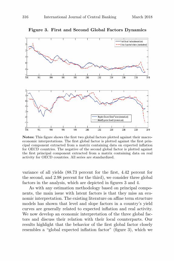
Figure 3. First and Second Global Factors Dynamics

Notes: This figure shows the first two global factors plotted against their macro-economic interpretations. The first global factor is plotted against the first prin-cipal component extracted from a matrix containing data on expected inflationfor OECD countries. The negative of the second global factor is plotted againstthe first principal component extracted from a matrix containing data on realactivity for OECD countries. All series are standardized.

variance of all yields (88.73 percent for the first, 4.42 percent forthe second, and 2.98 percent for the third), we consider three globalfactors in the analysis, which are depicted in figures 3 and 4.

As with any estimation methodology based on principal compo-nents, the main issue with latent factors is that they miss an eco-nomic interpretation. The existing literature on affine term structuremodels has shown that level and slope factors in a country’s yieldcurves are generally related to expected inflation and real activity.We now develop an economic interpretation of the three global fac-tors and discuss their relation with their local counterparts. Ourresults highlight that the behavior of the first global factor closelyresembles a “global expected inflation factor” (figure 3), which we


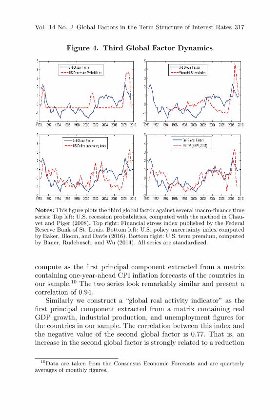
Figure 4. Third Global Factor Dynamics

Notes: This figure plots the third global factor against several macro-finance timeseries: Top left: U.S. recession probabilities, computed with the method in Chau-vet and Piger (2008). Top right: Financial stress index published by the FederalReserve Bank of St. Louis. Bottom left: U.S. policy uncertainty index computedby Baker, Bloom, and Davis (2016). Bottom right: U.S. term premium, computedby Bauer, Rudebusch, and Wu (2014). All series are standardized.

compute as the first principal component extracted from a matrixcontaining one-year-ahead CPI inflation forecasts of the countries inour sample.10 The two series look remarkably similar and present acorrelation of 0.94.

Similarly we construct a “global real activity indicator” as thefirst principal component extracted from a matrix containing realGDP growth, industrial production, and unemployment figures forthe countries in our sample. The correlation between this index andthe negative value of the second global factor is 0.77. That is, anincrease in the second global factor is strongly related to a reduction

10Data are taken from the Consensus Economic Forecasts and are quarterlyaverages of monthly figures.


in expected growth. In fact, as shown in the bottom panel of figure 3,the global real activity factor manages to capture the three down-ward movements displayed by the negative value of the second globalfactor: These spells occur between 1990 and 1995, between 2000 and2005, and finally during the Great Recession. For this last period,however, the global real activity factor drops by less.

Regarding the third global factor, its correlation with the averageof the local curvatures is 0.43. Finding an economic interpretationfor the third global factor is, however, a novel task. Figure 4 plots thethird global factor together with several related macro-finance series:probability of recession in the United States computed by Chauvetand Piger (2008) (top left), a financial stress index published by theFederal Reserve Bank of St. Louis (top right), the U.S. policy uncer-tainty index derived by Baker, Bloom, and Davis (2016) (bottomleft), and the U.S. term premium computed by Bauer, Rudebusch,and Wu (2014). Overall, the dynamics of the third global factor showa decrease in the first part of the sample (up to 2000) and an increasein the second part, especially around 2007. The graphs show thatthe peak of the third global factor in 2007 coincides with a sharpincrease in both the U.S. recession probability and the policy uncer-tainty index. It also precedes the peak in the financial stress indexand thus anticipates this financial/liquidity risk episode. We latercomment on the relation with the U.S. term premium.

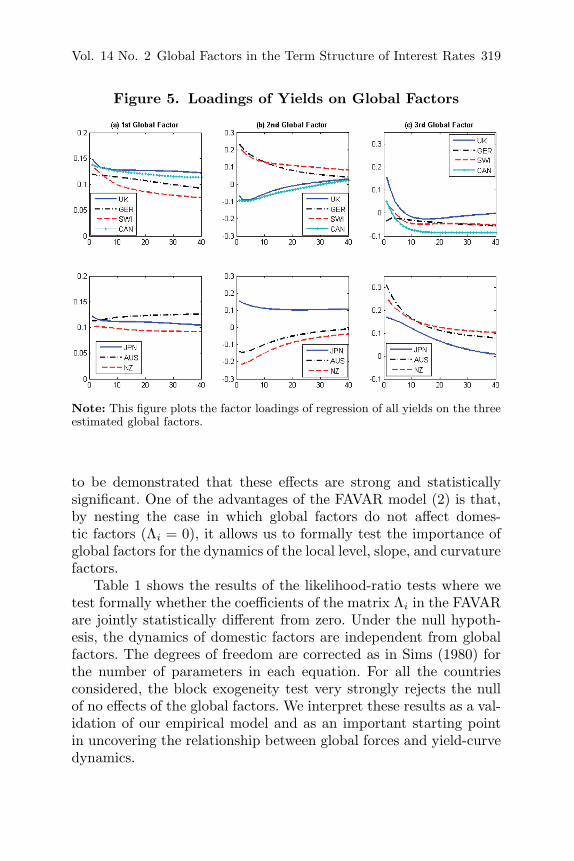
As a last piece of interpretation of our global factors, we regressyields on the three global factors to gauge the shape of the impliedloadings. As figure 5 shows, the loadings on the first global factor arerelatively flat and persistent, resembling a classical global level fac-tor. The loadings on the second global factor differ across countries,exhibiting either increasing or decreasing patterns. Finally, loadingson the third factor are all decreasing and, in most cases, convex.These results are consistent with those in Bauer and Dıez de losRios (2014). While not reported, we also find that a fourth globalfactor emerges as a global slope factor. Subsequent results in thispaper are robust to the inclusion of a fourth global factor in ouranalysis.

6.2 Model Performance

While there are many sound economic arguments to support theidea that global factors influence domestic term structures, it needs


Figure 5. Loadings of Yields on Global Factors

Note: This figure plots the factor loadings of regression of all yields on the threeestimated global factors.

to be demonstrated that these effects are strong and statisticallysignificant. One of the advantages of the FAVAR model (2) is that,by nesting the case in which global factors do not affect domes-tic factors (Λi = 0), it allows us to formally test the importance ofglobal factors for the dynamics of the local level, slope, and curvaturefactors.

Table 1 shows the results of the likelihood-ratio tests where wetest formally whether the coefficients of the matrix Λi in the FAVARare jointly statistically different from zero. Under the null hypoth-esis, the dynamics of domestic factors are independent from globalfactors. The degrees of freedom are corrected as in Sims (1980) forthe number of parameters in each equation. For all the countriesconsidered, the block exogeneity test very strongly rejects the nullof no effects of the global factors. We interpret these results as a val-idation of our empirical model and as an important starting pointin uncovering the relationship between global forces and yield-curvedynamics.


Table 1. Block Exogeneity Test

Likelihood-Ratio Test

Country Stat. p-value

JPN 40.11 0.00UK 106.81 0.00

GER 128.17 0.00SWI 96.06 0.00CAN 74.20 0.00AUS 95.26 0.00NZL 153.67 0.00

Notes: This table shows the p-values associated with the likelihood-ratio statis-tics testing no significance of global factors Ft on domestic factors Xit, as specifiedin our FAVAR term structure model. We apply the Sims (1980) correction on thelikelihood-ratio test, correcting degrees of freedom for the number of regressors perequation.

To evaluate the fit of the model, table 2 shows the root mean

square fitting error of yields, i.e.,

(√1

T×N

∑t

∑n

(ynit − yn

it)2)

. The

fit of the model is excellent. The typical fitting errors range between1.4 and 4.2 basis points, with New Zealand, Germany, and Japanexhibiting the best fit.

6.3 How Important Are Global Factorsfor Domestic Factors and Yields?

In our model, we have implicitly assumed a hierarchical structure,in which country yields depend only on country-specific factors, butthese are in turn affected by the dynamics of global forces. Anyinfluence of global factors on domestic interest rates can thus comeonly through their effect on the domestic level, slope, and curvaturefactor. To understand the effect of global forces on country yields,in this section we use the FAVAR model to perform two exercises.First, we analyze the impulse responses of domestic factors to globalshocks. Then, we compute the variance decomposition of the threelocal factors included in the vector Xit.


Table 2. Model Fit

Fit of Affine Term Structure Model

Country RMSE

JPN 0.0180UK 0.0417

GER 0.0199SWI 0.0316CAN 0.0352AUS 0.0278NZL 0.0143

Note: This table shows the root mean square fitting error (square root of the min-imized value of the objective function of the affine term structure model) for eachcountry, in percentage points.

To perform these exercises, global shocks are identified with asimple Cholesky decomposition. Using the macroeconomic interpre-tation of the global factors, we order the second global factor, cap-turing global real activity, as first, the third global factor as second,and the global expected inflation factor last. Notice, however, thatalternative factor orderings do not affect our results.

Figure 6 shows the dynamic response of local yield factors toglobal forces in the case of the United Kingdom.11 The unreportedresults for other countries give a similar picture.12 Global factorshave a sizable and persistent effect on domestic factors. A positiveinnovation to the second global factor has a negative effect on thedomestic level and a positive effect on the slope factor. This is con-sistent with the idea that a global boom tends to induce both animprovement in the domestic cycle and an increase in the domesticinflation risk. Notice that both effects are delayed and very persis-tent. An increase in the third global factor instead causes an increasein domestic curvature and slope and a reduction in the domesticlevel factor. This increase in domestic curvature is common acrossall countries. Notice that the effect of this shock is small on impact

11Confidence intervals are obtained using the bootstrap-after-bootstrapmethod as described in Kilian (1998).

12All results are available upon request from the authors.


Figure 6. Responses of Local Yield Factors to GlobalFactors in the United Kingdom

Notes: This figure shows the responses of the three local factors (level, slope,and curvature) contained in Xit to shocks to the three global factors. Impulseresponses are plotted for a horizon of forty periods. Dotted lines represent a+/−1 standard deviation confidence interval. Results are reported for the UnitedKingdom only.

but more persistent, as it remains different from zero for more thantwenty quarters. Finally, a shock to the first global factor causes anincrease in the countries’ level factor (i.e., the countries’ inflation riskfactor), while it has a small and heterogeneous effect on countries’slope and curvature factors.

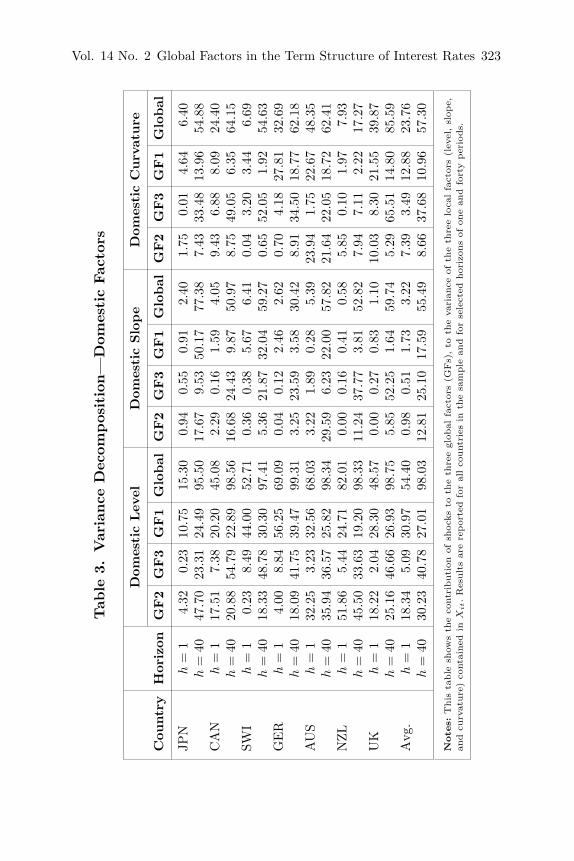
Table 3 shows the contribution of global shocks to the varianceof the local factors at two forecasting horizons: one quarter and fortyquarters. At short horizons, country-specific shocks explain most ofthe variance of the three local factors, but global factors are far fromunimportant. Global factors explain, on average, 54 percent of the


Tab

le3.

Var

iance

Dec

ompos

itio

n—

Dom

estic

Fac

tors

Dom

esti

cLev

elD

omes

tic

Slo

pe

Dom

esti

cC

urv

ature

Cou

ntr

yH

oriz

onG

F2

GF3

GF1

Glo

bal

GF2

GF3

GF1

Glo

bal

GF2

GF3

GF1

Glo

bal

JPN

h=

14.

320.

2310

.75

15.3

00.

940.

550.

912.

401.

750.

014.

646.

40h

=40

47.7

023

.31

24.4

995

.50

17.6

79.

5350

.17

77.3

87.

4333

.48

13.9

654

.88

CA

Nh

=1

17.5

17.

3820

.20

45.0

82.

290.

161.

594.

059.

436.

888.

0924

.40

h=

4020

.88

54.7

922

.89

98.5

616

.68

24.4

39.

8750

.97

8.75

49.0

56.

3564

.15

SWI

h=

10.

238.

4944

.00

52.7

10.

360.

385.

676.

410.

043.

203.

446.

69h

=40

18.3

348

.78

30.3

097

.41

5.36

21.8

732

.04

59.2

70.

6552

.05

1.92

54.6

3G

ER

h=

14.

008.

8456

.25

69.0

90.

040.

122.

462.

620.

704.

1827

.81

32.6

9h

=40

18.0

941

.75

39.4

799

.31

3.25

23.5

93.

5830

.42

8.91

34.5

018

.77

62.1

8A

US

h=

132

.25

3.23

32.5

668

.03

3.22

1.89

0.28

5.39

23.9

41.

7522

.67

48.3

5h

=40

35.9

436

.57

25.8

298

.34

29.5

96.

2322

.00

57.8

221

.64

22.0

518

.72

62.4

1N

ZL

h=

151

.86

5.44

24.7

182

.01

0.00

0.16

0.41

0.58

5.85

0.10

1.97

7.93

h=

4045

.50

33.6

319

.20

98.3

311

.24

37.7

73.

8152

.82

7.94

7.11

2.22

17.2

7U

Kh

=1

18.2

22.

0428

.30

48.5

70.

000.

270.

831.

1010

.03

8.30

21.5

539

.87

h=

4025

.16

46.6

626

.93

98.7

55.

8552

.25

1.64

59.7

45.

2965

.51

14.8

085

.59

Avg

.h

=1

18.3

45.

0930

.97

54.4

00.

980.

511.

733.

227.

393.

4912

.88

23.7

6h

=40

30.2

340

.78

27.0

198

.03

12.8

125

.10

17.5

955

.49

8.66

37.6

810

.96

57.3

0

Note

s:T

his

table

show

sth

eco

ntri

buti

onof

shoc

ksto

the

thre

egl

obal

fact

ors

(GFs)

,to

the

vari

ance

ofth

eth

ree

loca

lfa

ctor

s(l

evel

,sl

ope,

and

curv

ature

)co

ntai

ned

inX

it.R

esult

sar

ere

por

ted

for

allco

unt

ries

inth

esa

mple

and

for

sele

cted

hor

izon

sof

one

and

fort

yper

iods.


Figure 7. Contribution of Global Shocks to theYield-Curve Dynamics

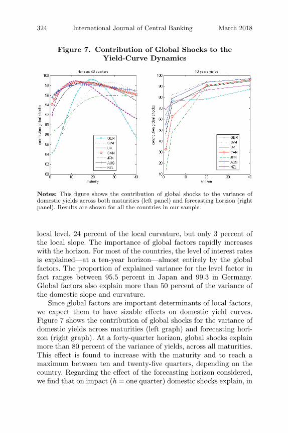
Notes: This figure shows the contribution of global shocks to the variance ofdomestic yields across both maturities (left panel) and forecasting horizon (rightpanel). Results are shown for all the countries in our sample.

local level, 24 percent of the local curvature, but only 3 percent ofthe local slope. The importance of global factors rapidly increaseswith the horizon. For most of the countries, the level of interest ratesis explained—at a ten-year horizon—almost entirely by the globalfactors. The proportion of explained variance for the level factor infact ranges between 95.5 percent in Japan and 99.3 in Germany.Global factors also explain more than 50 percent of the variance ofthe domestic slope and curvature.

Since global factors are important determinants of local factors,we expect them to have sizable effects on domestic yield curves.Figure 7 shows the contribution of global shocks for the variance ofdomestic yields across maturities (left graph) and forecasting hori-zon (right graph). At a forty-quarter horizon, global shocks explainmore than 80 percent of the variance of yields, across all maturities.This effect is found to increase with the maturity and to reach amaximum between ten and twenty-five quarters, depending on thecountry. Regarding the effect of the forecasting horizon considered,we find that on impact (h = one quarter) domestic shocks explain, in


most countries, most of the ten-year yield. Already after four quar-ters, however, global shocks dominate the variance decomposition ofthe ten-year yield, showing that the effect of global shocks tends tobe large but delayed.

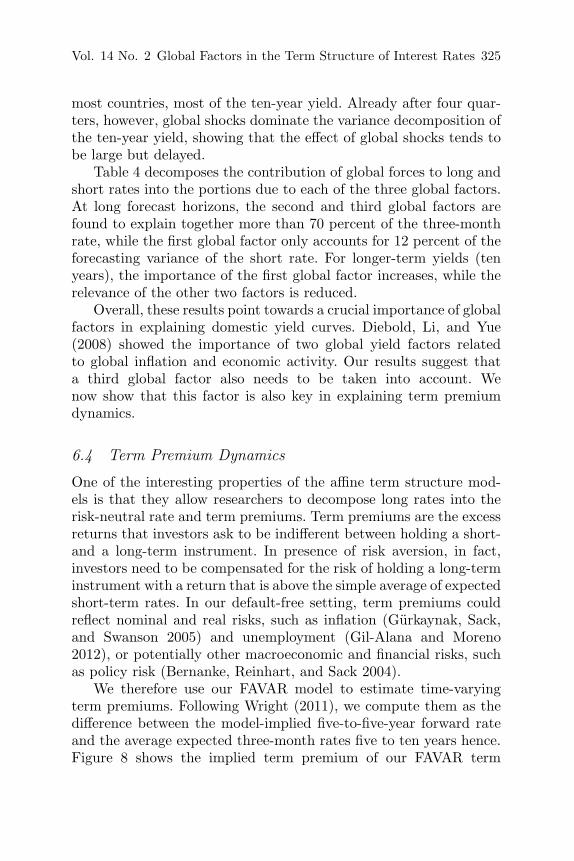
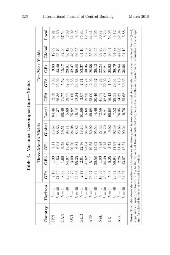
Table 4 decomposes the contribution of global forces to long andshort rates into the portions due to each of the three global factors.At long forecast horizons, the second and third global factors arefound to explain together more than 70 percent of the three-monthrate, while the first global factor only accounts for 12 percent of theforecasting variance of the short rate. For longer-term yields (tenyears), the importance of the first global factor increases, while therelevance of the other two factors is reduced.

Overall, these results point towards a crucial importance of globalfactors in explaining domestic yield curves. Diebold, Li, and Yue(2008) showed the importance of two global yield factors relatedto global inflation and economic activity. Our results suggest thata third global factor also needs to be taken into account. Wenow show that this factor is also key in explaining term premiumdynamics.

6.4 Term Premium Dynamics

One of the interesting properties of the affine term structure mod-els is that they allow researchers to decompose long rates into therisk-neutral rate and term premiums. Term premiums are the excessreturns that investors ask to be indifferent between holding a short-and a long-term instrument. In presence of risk aversion, in fact,investors need to be compensated for the risk of holding a long-terminstrument with a return that is above the simple average of expectedshort-term rates. In our default-free setting, term premiums couldreflect nominal and real risks, such as inflation (Gurkaynak, Sack,and Swanson 2005) and unemployment (Gil-Alana and Moreno2012), or potentially other macroeconomic and financial risks, suchas policy risk (Bernanke, Reinhart, and Sack 2004).

We therefore use our FAVAR model to estimate time-varyingterm premiums. Following Wright (2011), we compute them as thedifference between the model-implied five-to-five-year forward rateand the average expected three-month rates five to ten years hence.Figure 8 shows the implied term premium of our FAVAR term


Tab

le4.

Var

iance

Dec

ompos

itio

n—

Yie

lds

Thre

e-M

onth

Yie

lds

Ten

-Yea

rY

ield

s

Cou

ntr

yH

oriz

onG

F2

GF3

GF1

Glo

bal

Loca

lG

F2

GF3

GF1

Glo

bal

Loca

l

JPN

h=

17.

101.

337.

1115

.54

84.4

62.

190.

069.

8312

.09

87.9

1h

=40

71.0

911

.53

6.01

88.6

311

.37

26.3

825

.92

43.4

095

.70

4.30

CA

Nh

=1

8.33

1.60

9.59

19.5

180

.49

11.7

75.

5215

.17

32.4

667

.54

h=

4023

.65

54.9

715

.49

94.1

15.

8919

.77

47.5

428

.81

96.1

23.

88SW

Ih

=1

0.79

3.09

20.2

024

.08

75.9

20.

066.

5642

.37

48.9

851

.02

h=

4022

.63

55.3

56.

8484

.82

15.1

812

.34

24.3

359

.88

96.5

53.

45G

ER

h=

12.

772.

6112

.76

18.1

481

.86

3.07

7.71

53.3

764

.16

35.8

4h

=40

13.6

647

.62

23.0

484

.32

15.6

819

.28

27.7

440

.35

87.3

712

.63

AU

Sh

=1

26.2

75.

1119

.53

50.9

249

.08

25.0

02.

0328

.56

55.5

944

.41

h=

4049

.34

30.5

815

.62

95.5

44.

4630

.46

36.3

730

.12

96.9

53.

05N

ZL

h=

118

.38

1.83

7.24

27.4

472

.56

41.7

55.

2422

.24

69.2

330

.77

h=

4040

.58

44.4

96.

7391

.79

8.21

42.0

222

.02

27.2

191

.25

8.75

UK

h=

15.

930.

253.

749.

9290

.08

16.4

21.

5928

.92

46.9

453

.06

h=

4023

.57

56.9

411

.97

92.4

87.

5229

.55

28.5

436

.79

94.8

85.

12A

vg.

h=

19.

942.

2611

.45

23.6

576

.35

14.3

24.

1028

.64

47.0

652

.94

h=

4034

.93

43.0

712

.24

90.2

49.

7625

.68

30.3

538

.08

94.1

25.

88

Note

s:T

his

table

show

sth

eco

ntri

buti

onof

shoc

ksto

the

thre

egl

obal

fact

ors,

thei

rsu

m,an

dth

eco

ntri

buti

onof

the

thre

elo

calfa

ctor

s(l

evel

,sl

ope,

and

curv

ature

)co

ntai

ned

inX

it

toth

eva

rian

ceof

thre

e-m

onth

and

ten-y

ear

yiel

ds.

Res

ult

sar

ere

por

ted

for

allco

unt

ries

inth

esa

mple

and

for

sele

cted

hor

izon

sof

one

and

fort

yper

iods.


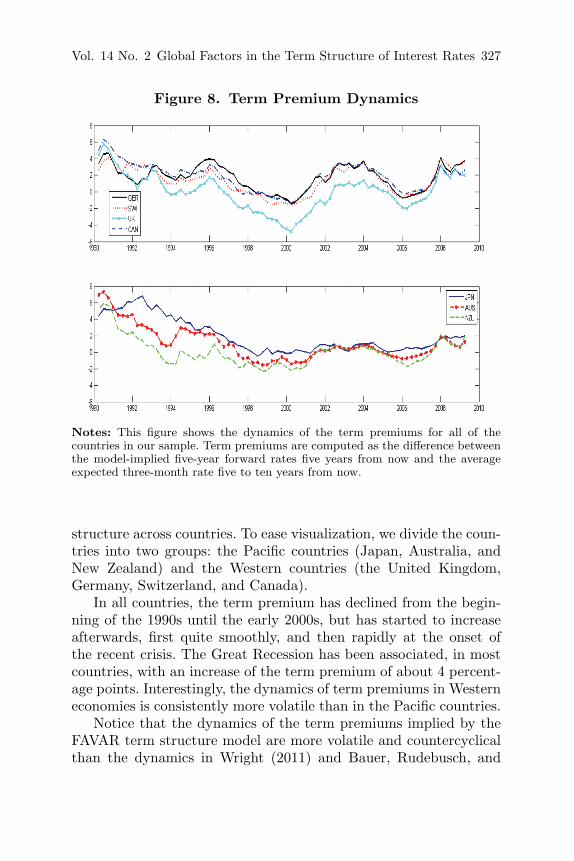
Figure 8. Term Premium Dynamics

Notes: This figure shows the dynamics of the term premiums for all of thecountries in our sample. Term premiums are computed as the difference betweenthe model-implied five-year forward rates five years from now and the averageexpected three-month rate five to ten years from now.

structure across countries. To ease visualization, we divide the coun-tries into two groups: the Pacific countries (Japan, Australia, andNew Zealand) and the Western countries (the United Kingdom,Germany, Switzerland, and Canada).

In all countries, the term premium has declined from the begin-ning of the 1990s until the early 2000s, but has started to increaseafterwards, first quite smoothly, and then rapidly at the onset ofthe recent crisis. The Great Recession has been associated, in mostcountries, with an increase of the term premium of about 4 percent-age points. Interestingly, the dynamics of term premiums in Westerneconomies is consistently more volatile than in the Pacific countries.

Notice that the dynamics of the term premiums implied by theFAVAR term structure model are more volatile and countercyclicalthan the dynamics in Wright (2011) and Bauer, Rudebusch, and


Wu (2014). The higher volatility with respect to Wright (2011) wasexpected, because we correct the FAVAR estimates for the small-sample bias, which tend to make the estimated system less persis-tent. The higher volatility with respect to Bauer, Rudebusch, andWu (2014), instead, suggests that the presence of global factors fur-ther increases the volatility of the expectations of future short-terminterest rates, especially at longer horizons. Notice also that the termpremium can become negative for some countries, especially afterthe mid-1990s. As Campbell, Sunderam, and Viceira (2013) haveshown, this situation can arise under a negative correlation betweenstock market and bond market returns. In this instance, long-termbonds can hedge against stock market losses and, in general, againstthe backdrop of recession episodes. As a result, investors are eagerto accept lower returns on long-term bonds vis a vis short-termbonds.

In general, the dynamics of the term premiums have been asso-ciated with the so-called inflation risk. The declining pattern in theearly part in figure 8 would therefore be evidence that central banks,with the adoption of an explicit target for inflation, have managedto anchor inflationary expectations and therefore reduced term pre-miums. The increase observed in the last part of the sample, how-ever, suggests that there might be something more to it. Thus, itis important to ask whether these term premium dynamics are dueto developments in the domestic economies or to global develop-ments, because the implications for policymakers may be strikinglydifferent. This is a task that we perform in the following section.

6.5 Global Factors and Term Premium Dynamics

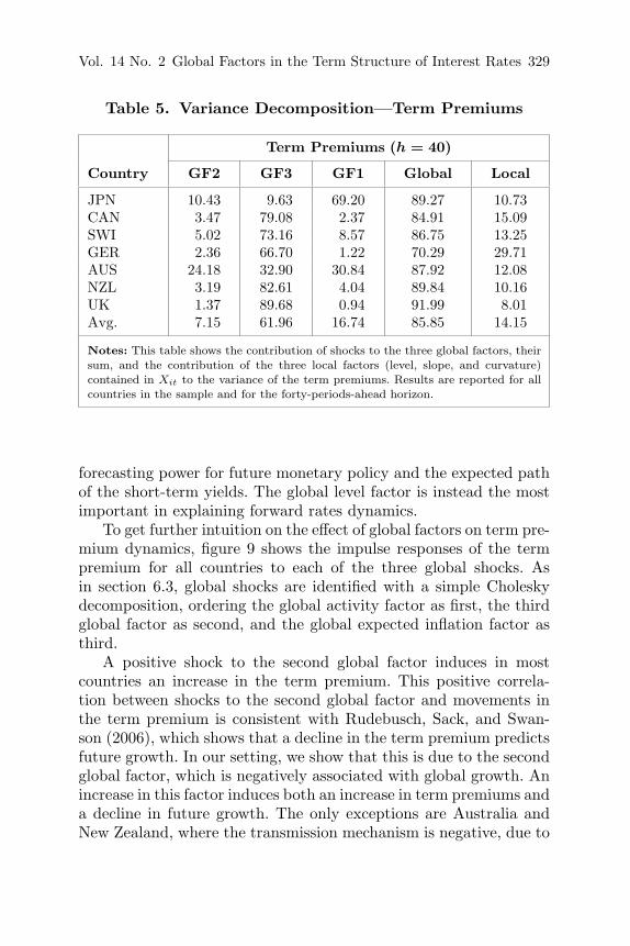
To understand the importance of global forces for term premiumdynamics, table 5 reports the variance decompositions in term pre-mium dynamics. The contribution of global factors to term premiumvariations ranges between 70 percent in the case of Germany and 92percent in the case of the United Kingdom. The third global factoris, on average, the most important in explaining term premium vari-ation, as it explains around 62 percent of the total variance at theforty-quarter horizon. This happens mainly because shocks to thethird global factor explain most of the variance of the risk-neutralrate (table 6), which indicates that the third global factor has a large


Table 5. Variance Decomposition—Term Premiums

Term Premiums (h = 40)

Country GF2 GF3 GF1 Global Local

JPN 10.43 9.63 69.20 89.27 10.73CAN 3.47 79.08 2.37 84.91 15.09SWI 5.02 73.16 8.57 86.75 13.25GER 2.36 66.70 1.22 70.29 29.71AUS 24.18 32.90 30.84 87.92 12.08NZL 3.19 82.61 4.04 89.84 10.16UK 1.37 89.68 0.94 91.99 8.01Avg. 7.15 61.96 16.74 85.85 14.15

Notes: This table shows the contribution of shocks to the three global factors, theirsum, and the contribution of the three local factors (level, slope, and curvature)contained in Xit to the variance of the term premiums. Results are reported for allcountries in the sample and for the forty-periods-ahead horizon.

forecasting power for future monetary policy and the expected pathof the short-term yields. The global level factor is instead the mostimportant in explaining forward rates dynamics.

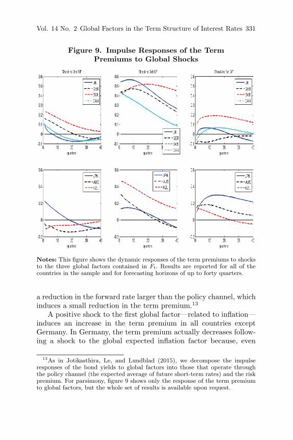
To get further intuition on the effect of global factors on term pre-mium dynamics, figure 9 shows the impulse responses of the termpremium for all countries to each of the three global shocks. Asin section 6.3, global shocks are identified with a simple Choleskydecomposition, ordering the global activity factor as first, the thirdglobal factor as second, and the global expected inflation factor asthird.

A positive shock to the second global factor induces in mostcountries an increase in the term premium. This positive correla-tion between shocks to the second global factor and movements inthe term premium is consistent with Rudebusch, Sack, and Swan-son (2006), which shows that a decline in the term premium predictsfuture growth. In our setting, we show that this is due to the secondglobal factor, which is negatively associated with global growth. Anincrease in this factor induces both an increase in term premiums anda decline in future growth. The only exceptions are Australia andNew Zealand, where the transmission mechanism is negative, due to


Tab

le6.

Var

iance

Dec

ompos

itio

n—

For

war

dan

dR

isk-N

eutr

alR

ates

For

war

dR

ates

(h=

40)

Ris

k-N

eutr

alR

ates

(h=

40)

Cou

ntr

yG

F2

GF3

GF1

Glo

bal

Loca

lG

F2

GF3

GF1

Glo

bal

Loca

l

JPN

12.1

123

.62

57.0

892

.82

7.18

32.1

259

.74

5.43

97.2

92.

71C

AN

18.4

436

.45

34.7

689

.65

10.3

55.

9282

.92

11.1

299

.97

0.03

SWI

3.96

1.95

75.2

081

.10

18.9

07.

9187

.59

0.28

95.7

74.

23G

ER

14.3

59.

1125

.23

48.6

851

.32

5.36

79.9

511

.22

96.5

33.

47A

US

26.6

634

.83

33.0

194

.49

5.51

6.79

85.2

67.

9599

.99

0.01

NZL

34.3

412

.67

32.2

079

.22

20.7

84.

8087

.66

7.54

99.9

90.

01U

K31

.19

10.2

541

.22

82.6

617

.34

4.94

84.6

410

.36

99.9

40.

06A

vg.

20.1

518

.41

42.6

781

.23

18.7

79.

6981

.11

7.70

98.5

01.

50

Note

s:T

his

table

show

sth

eco

ntri

buti

onof

shoc

ksto

the

thre

egl

obal

fact

ors,

thei

rsu

m,an

dth

eco

ntri

buti

onof

the

thre

elo

calfa

ctor

s(l

evel

,sl

ope,

and

curv

ature

)co

ntai

ned

inX

it

toth

eva

rian

ceof

the

forw

ard

inte

rest

rate

san

dth

eri

sk-n

eutr

alin

tere

stra

tes.

Res

ult

sar

ere

por

ted

for

allco

unt

ries

inth

esa

mple

and

for

the

fort

y-per

iods-

ahea

dhor

izon

.


Figure 9. Impulse Responses of the TermPremiums to Global Shocks

Notes: This figure shows the dynamic responses of the term premiums to shocksto the three global factors contained in Ft. Results are reported for all of thecountries in the sample and for forecasting horizons of up to forty quarters.

a reduction in the forward rate larger than the policy channel, whichinduces a small reduction in the term premium.13

A positive shock to the first global factor—related to inflation—induces an increase in the term premium in all countries exceptGermany. In Germany, the term premium actually decreases follow-ing a shock to the global expected inflation factor because, even

13As in Jotikasthira, Le, and Lundblad (2015), we decompose the impulseresponses of the bond yields to global factors into those that operate throughthe policy channel (the expected average of future short-term rates) and the riskpremium. For parsimony, figure 9 shows only the response of the term premiumto global factors, but the whole set of results is available upon request.


though long rates and the forward rate increase after the shock, therisk-neutral rates increase by more on impact. The fact that thepolicy channel dominates in Germany is symptomatic of the highcredibility of its monetary policy stance. In the other countries,the policy channel response is relatively more muted on impact,compared with Germany, although it increases over time, leadingthen to a subsequent reduction in term premiums over the longerhorizon.

Finally, a positive shock to the third global factor produces anincrease in term premiums across all countries. The effect is rela-tively large, especially in Western countries, and quite persistent, asit usually lasts more than thirty quarters. Interestingly, these resultsare consistent with the bottom-right panel of figure 4, which plotsthe third global factor against the U.S. term premium implied bythe model in Bauer, Rudebusch, and Wu (2014). It reveals that thethird global factor captures the dynamics of the term premium veryclosely. This is especially the case at the end of the sample, coin-ciding with the onset of the financial crisis. In the next section wefurther explore the role of the third global factor during this lattersubperiod.

7. Robustness Checks

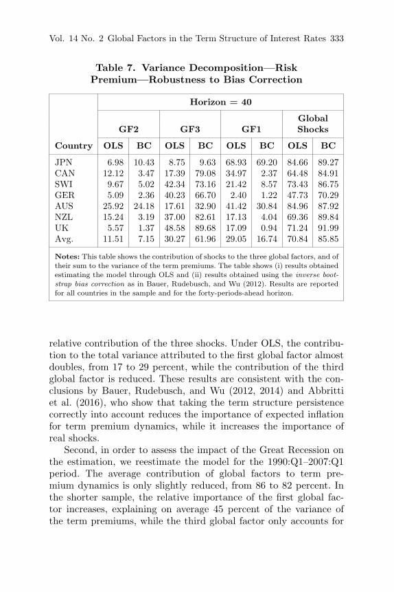
We test the robustness of our results with three exercises. First, tounderstand to what extent bias correction affects our conclusions,we compare the main results reported above (under bias correc-tion) with analogs obtained without bias correction. As in Bauer,Rudebusch, and Wu (2012, 2014), we find that bias correction hasimportant effects on the identification of the term premium. For allcountries, the term premium identified with simple OLS presentsa clearer downward-sloping trend; it is less volatile/countercyclicaland does not increase as much during the Great Recession. Theconclusions about the importance of global factors, however, holdindependently of the bias correction in the state process (table 7).Bias correction slightly increases the total contribution of globalshocks, but in the model estimated with simple OLS, global shocksstill account, on average, for more than 70 percent of the total vari-ance in the term premiums. However, bias correction affects the


Table 7. Variance Decomposition—RiskPremium—Robustness to Bias Correction

Horizon = 40

GlobalGF2 GF3 GF1 Shocks

Country OLS BC OLS BC OLS BC OLS BC

JPN 6.98 10.43 8.75 9.63 68.93 69.20 84.66 89.27CAN 12.12 3.47 17.39 79.08 34.97 2.37 64.48 84.91SWI 9.67 5.02 42.34 73.16 21.42 8.57 73.43 86.75GER 5.09 2.36 40.23 66.70 2.40 1.22 47.73 70.29AUS 25.92 24.18 17.61 32.90 41.42 30.84 84.96 87.92NZL 15.24 3.19 37.00 82.61 17.13 4.04 69.36 89.84UK 5.57 1.37 48.58 89.68 17.09 0.94 71.24 91.99Avg. 11.51 7.15 30.27 61.96 29.05 16.74 70.84 85.85

Notes: This table shows the contribution of shocks to the three global factors, and oftheir sum to the variance of the term premiums. The table shows (i) results obtainedestimating the model through OLS and (ii) results obtained using the inverse boot-strap bias correction as in Bauer, Rudebusch, and Wu (2012). Results are reportedfor all countries in the sample and for the forty-periods-ahead horizon.

relative contribution of the three shocks. Under OLS, the contribu-tion to the total variance attributed to the first global factor almostdoubles, from 17 to 29 percent, while the contribution of the thirdglobal factor is reduced. These results are consistent with the con-clusions by Bauer, Rudebusch, and Wu (2012, 2014) and Abbrittiet al. (2016), who show that taking the term structure persistencecorrectly into account reduces the importance of expected inflationfor term premium dynamics, while it increases the importance ofreal shocks.

Second, in order to assess the impact of the Great Recession onthe estimation, we reestimate the model for the 1990:Q1–2007:Q1period. The average contribution of global factors to term pre-mium dynamics is only slightly reduced, from 86 to 82 percent. Inthe shorter sample, the relative importance of the first global fac-tor increases, explaining on average 45 percent of the variance ofthe term premiums, while the third global factor only accounts for


Table 8. Variance Decomposition—TermPremiums—Subsample 1990:Q1–2007:Q1




Notes: This table shows the contribution of shocks to the three global factors, theirsum, and the contribution of the three local factors (level, slope, and curvature) con-tained in Xit to the variance of the term premiums when the model is estimated forthe period 1990:Q1–2007:Q1 only. Results are reported for all countries in the sampleand for the forty-periods-ahead horizon.

13 percent of the total variance (table 8). This exercise confirmsprevious papers that attribute the decline of term premiums toexpected inflation until the early/mid-2000s. It also shows that theimportance of the third global factor is greatly diminished if weexclude the last part of the sample—the financial crisis period. Thus,it is the financial crisis that brings to the scene the key relevance ofthe third global factor triggering international yield-curve dynamics.

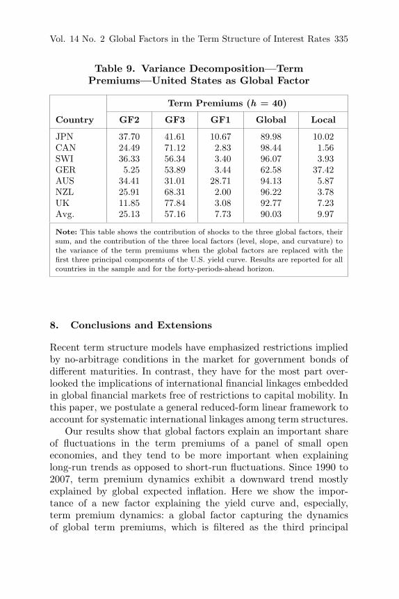
Third, we treat the U.S. factors as the global ones. This is justi-fied by the relevance of the United States in the global economy aswell as the importance of U.S. monetary policy in global financialmarkets (see, for instance, Jotikashtira, Le, and Lundblad 2015). Intable 9 we show the variance decomposition of the term premiumsacross countries. We find that global factors are still key to explainterm premium variations (around 90 percent) and that the thirdglobal factor, the U.S. curvature factor, is still the most important,explaining around 57 percent of the total variance. Nevertheless,with respect to the baseline model, it loses explanatory power infavor of the U.S. cycle factor.


Table 9. Variance Decomposition—TermPremiums—United States as Global Factor




Note: This table shows the contribution of shocks to the three global factors, theirsum, and the contribution of the three local factors (level, slope, and curvature) tothe variance of the term premiums when the global factors are replaced with thefirst three principal components of the U.S. yield curve. Results are reported for allcountries in the sample and for the forty-periods-ahead horizon.

8. Conclusions and Extensions

Recent term structure models have emphasized restrictions impliedby no-arbitrage conditions in the market for government bonds ofdifferent maturities. In contrast, they have for the most part over-looked the implications of international financial linkages embeddedin global financial markets free of restrictions to capital mobility. Inthis paper, we postulate a general reduced-form linear framework toaccount for systematic international linkages among term structures.

Our results show that global factors explain an important shareof fluctuations in the term premiums of a panel of small openeconomies, and they tend to be more important when explaininglong-run trends as opposed to short-run fluctuations. Since 1990 to2007, term premium dynamics exhibit a downward trend mostlyexplained by global expected inflation. Here we show the impor-tance of a new factor explaining the yield curve and, especially,term premium dynamics: a global factor capturing the dynamicsof global term premiums, which is filtered as the third principal


component of the international yield curves. Interestingly, this fac-tor takes center stage when explaining the dynamics of the recentcrisis. During this time, monetary policy has been extraordinarilyexpansionary, sharply and immediately lowering interest rate expec-tations. In future work, we intend to examine the term structureimplications of the zero—or near zero—interest rate lower boundin the years beyond the sample period in this paper. Analyzing theinternational spillovers of these ongoing unconventional policies isdefinitely a worthwhile exercise.

References

Abbritti, M., L. Gil-Alana, Y. Lovcha, and A. Moreno. 2016. “TermStructure Persistence.” Journal of Financial Econometrics 14(2): 331–52.

Ang, A., and M. Piazzesi. 2003. “A No-Arbitrage Vector Autore-gression of Term Structure Dynamics with Macroeconomic andLatent Variables.” Journal of Monetary Economics 50 (4): 745–87.

Baker, S. R., N. Bloom, and S. J. Davis. 2016. “Measuring Eco-nomic Policy Uncertainty.” Quarterly Journal of Economics131 (4): 1593–1636.

Bauer, G., and A. Dıez de los Rios. 2014. “An InternationalDynamic Term Structure Model with Economic Restrictions andUnspanned Risks.” Working Paper, Bank of Canada.

Bauer, M. D., G. D. Rudebusch, and J. Cynthia Wu. 2012. “Cor-recting Estimation Bias in Dynamic Term Structure Models.”Journal of Business and Economic Statistics 30 (3): 454–67.

———. 2014. “Term Premia and Inflation Uncertainty: Empiri-cal Evidence from an International Panel Dataset: Comment.”American Economic Review 104 (1): 323–37.

Bekaert, G., S. Cho, and A. Moreno. 2010. “New Keynesian Macro-economics and the Term Structure.” Journal of Money, Creditand Banking 42 (1): 33–62.

Bernanke, B. S. 2006. “Remarks before the Economic Club of NewYork.” New York, March 20.

Bernanke, B., J. Boivin, and P. Eliasz. 2005. “Measuring the Effectsof Monetary Policy: A Factor-Augmented Vector Autoregressive


(FAVAR) Approach.” Quarterly Journal of Economics 120 (1):387–422.

Bernanke, B., V. R. Reinhart, and B. P. Sack. 2004. “Monetary Pol-icy Alternatives at the Zero Bound: An Empirical Assessment.”Brookings Papers on Economic Activity 35 (2): 1–100.

Campbell, J. Y., A. Sunderam, and L. M. Viceira. 2013. “Infla-tion Bets or Deflation Hedges? The Changing Risks of NominalBonds.” NBER Working Paper No. 14701.

Chauvet, M., and J. Piger. 2008. “A Comparison of the Real-TimePerformance of Business Cycle Dating Methods.” Journal ofBusiness and Economic Statistics 26 (1): 42–49.

Dell’Erba, S., and S. Sola. 2016. “Does Fiscal Policy Affect InterestRates? Evidence from a Factor-Augmented Panel.” B.E. Journalof Macroeconomics 16 (2): 395–437.

Diebold, F. X., C. Li, and V. Z. Yue. 2008. “Global YieldCurve Dynamics and Interactions: A Dynamic Nelson–SiegelApproach.” Journal of Econometrics 146 (2): 351–63.

Dıez de los Rıos, A. 2011. “Internationally Affine Term StructureModels.” Spanish Review of Financial Economics 9 (1): 31–34.

———. 2015. “A New Linear Estimator for Gaussian Dynamic TermStructure Models.” Journal of Business and Economic Statistics33 (2): 282–95.

Duffee, G. R. 1996. “Idiosyncratic Variation of Treasury Bill Yields.”Journal of Finance 51 (2): 527–52.

———. 2008. “Information in (and not in) the Term Structure.”Review of Financial Studies 24 (9): 2895–2934.

Geweke, J. 1977. “The Dynamic Factor Analysis of Economic TimeSeries Models.” In Latent Variables in Socioeconomic Models, ed.D. J. Aigner and A. S. Goldberger, 365–83. Amsterdam: NorthHolland.

Gil-Alana, L., and A. Moreno. 2012. “Uncovering the US Term Pre-mium: An Alternative Route.” Journal of Banking and Finance36 (4): 1181–93.

Gurkaynak, R. S., B. Sack, and E. Swanson. 2005. “The Sensitivityof Long-Term Interest Rates to Economic News: Evidence andImplications for Macroeconomic Models.” American EconomicReview 95 (1): 425–36.


Hellerstein, R. 2011. “Global Bond Risk Premiums.” Staff ReportNo. 499, Federal Reserve Bank of New York (June).

Joslin, S., M. Priebsch, and K. J. Singleton. 2014. “Risk Premiums inDynamic Term Structure Models with Unspanned Macro Risks.”Journal of Finance 69 (3): 1197–1233.

Jotikashtira, C., A. Le, and C. Lundblad. 2015. “Why Do TermStructures in Different Countries Co-move?” Journal of Finan-cial Economics 115 (1): 58–83.

Juneja, J. 2012. “Common Factors, Principal Components Analysis,and the Term Structure of Interest Rates.” International Reviewof Financial Analysis 24 (September): 48–56.

Kilian, L. 1998. “Small-Sample Confidence Intervals for ImpulseResponse Functions.” Review of Economics and Statistics 80 (2):218–30.

Ludvigson, S. L., and S. Ng. 2009. “Macro Factors in Bond RiskPremia.” Review of Financial Studies 22 (12): 5027–67.

Modugno, M., and N. Kleopatra. 2009. “The Forecasting Power ofInternational Yield Curve Linkages.” ECB Working Paper No.1044 (April).

Moench, E. 2008. “Forecasting the Yield Curve in a Data-Rich Envi-ronment: A No-Arbitrage Factor-Augmented VAR Approach.”Journal of Econometrics 146 (1): 26–43.

Pericoli, M., and M. Taboga. 2012. “Bond Risk Premia, Macro-economic Fundamentals and the Exchange Rate.” InternationalReview of Economics and Finance 22 (1): 42–65.

Perignon, C., D. R. Smith, and C. Villa. 2007. “Why CommonFactors in International Bond Returns Are Not So Common.”Journal of International Money and Finance 26 (2): 284–304.

Rudebusch, G. D., B. P. Sack, and E. T. Swanson. 2006. “Macroeco-nomic Implications of Changes in the Term Premium.” WorkingPaper No. 2006-46, Federal Reserve Bank of San Francisco.

Rudebusch, G. D., and E. T. Swanson. 2008. “Examining the BondPremium Puzzle with a DSGE Model.” Journal of MonetaryEconomics 55 (Supplement): S111–S126.

Sims, C. 1980. “Macroeconomics and Reality.” Econometrica 48 (1):1–48.


Spencer, P., and Z. Liu. 2010. “An Open-Economy Macro-FinanceModel of International Interdependence: The OECD, US and theUK.” Journal of Banking and Finance 34 (3): 667–80.

Stock, J. H., and M. W. Watson. 2005. “Implications of DynamicFactor Models for VAR Analysis.” NBER Working Paper No.11467.

———. 2002. “Forecasting Using Principal Components from aLarge Number of Predictors.” Journal of the American StatisticalAssociation 97 (460): 1167–79.

Wright, J. 2011. “Term Premia and Inflation Uncertainty: Empir-ical Evidence from an International Panel Dataset.” AmericanEconomic Review 101 (4): 1514–34.

global factors in the term structure of interest rates · explain term structure dynamics in the...

Documents