Term Structure Movements Implicit in AsianOption Prices ∗

Caio Almeida† Jose Vicente‡

September 15, 2009

Abstract

In this paper we implement dynamic term structure models thatadopt bonds and Asian options in the estimation process. The goalis to analyze the pricing and hedging implications of term structuremovements when options are (or not) included in the estimation pro-cess. We analyze how options affect the shape, risk premium andhedging structure of the dynamic factors. We find that the inclusionof options affects the loadings of the slope and curvature factors, andconsiderably changes the risk premium and hedging structure of alldynamic factors.

Keywords: Dynamic term structure models, latent factors, bond riskpremium, Asian option pricing.JEL classification: C51, G12.

∗We acknowledge useful comments from two anonymous referees, and from seminarparticipants at Catholic University of Rio de Janeiro, Federal University of Santa Cata-rina, Ibmec Business School SP, the Sixth Brazilian Meeting of Finance and XI Schoolof Time Series and Econometrics. The views expressed are those of the authors and donot necessarily reflect the views of the Central Bank of Brazil. The first author grate-fully acknowledges financial support given by CNPq-Brazil. Any remaining errors are ourresponsibility alone.†Graduate School of Economics, Getulio Vargas Foundation, e-mail: calmeida@fgv.br‡Faculdades Ibmec and Central Bank of Brazil, e-mail:jose.valentim@bcb.gov.br

1

1 Introduction

Interest rate Asian options are securities depending on the accumulated valueof the short-term rate. They are extremely useful hedging instruments forcorporations with volatile periodic cash flows. Nevertheless, despite the ex-istence of numerous theoretical results on the pricing of interest rate Asianoptions, previous research has been limited to cross-section option pricing1.In this paper, in contrast, we estimate multi-factor dynamic term structuremodels with joint data on bonds and interest rate Asian options. Our con-tribution is to analyze how these options affect the shape, risk premium andhedging structure of the corresponding dynamic term structure factors.

We implement two versions of a three-factor Gaussian model, one includ-ing only bonds in the estimation process and the other including bonds andoptions. As a robustness check of the hypothesis of constant volatility, wealso implement two versions of a three-factor affine model with one factordriving stochastic volatility (A1(3); Dai and Singleton, 2000). Closed-formformulas for bonds and Asian option prices allow efficient implementationof the Gaussian model. The A1(3) model is implemented via an adapta-tion of the Edgeworth expansion method proposed by Collin Dufresne andGoldstein (2002b) to price swaptions. The results of the A1(3) model qualita-tively confirm the results obtained with the Gaussian model with respect tothe shape of the term structure movements, and partially confirm the resultsconcerning the risk premium structure.

The two versions of the Gaussian and A1(3) models are estimated respec-tively by maximum likelihood and quasi maximum likelihood methods. Foreach model, the first version adopts only bond data (the bond version), andthe other combines bonds and data on at-the-money fixed-maturity options(the option version). Options appear to affect three dimensions of the dy-namic model: the loadings of term structure movements, bond risk premium

1Geman and Yor (1993) use the theory of Bessel processes to price Asian options undera Cox et al. (CIR, 1985) process. Longstaff (1995) use the Vasicek (1977) model to analyzethe properties of options on average interest rates. Leblanc and Scaillet (1998) presenttheoretical results on the pricing of interest rate Asian options under the Vasicek (1977)and CIR (1985) models, based on Laplace transforms. Cheuk and Vorst (1999) adopt aHull and White (1990) model. Dassios and Nagaradjasarma (2003) also adopt the CIR(1985) model, and use a series expansion representation method to price Asian options.Works using multi-factor models include Bakshi and Madan (1999), who use a two-factorCIR (1985) model, and Chacko and Das (2002), who apply Fourier transform methods toprice those options under general affine term structure models.

2

decomposition and dynamic first-order hedging terms2.Empirical results show that the level is a robust factor common to both

versions of each estimated model, while slope and curvature are less persis-tent under the option version of each model (see Figures 3 and 4). Thesemovements have much higher mean reversion rates under the option version.Thus, while the information contained in bonds and at-the-money optionsagree on the main factor driving term structure movements, the informationimplicit in those option prices suggest faster variations for the secondarymovements of the term structure.

Under the Gaussian model, the bond risk premium is slightly less volatilein the option version, and is more concentrated in the level factor. Underthe A1(3) model, the level factor makes a small contribution to the termstructure of risk premiums in both versions, while the slope factor appearsas the main factor driving the premium. Although each model has its ownrisk premium decomposition, both agree that when switching from the bondversion to the option version of each model, level has a greater effect on therisk premium decomposition while curvature has a smaller effect.

A comparison of the two estimated versions of the Gaussian model fur-ther reveals that the bond version better captures the term structure of bondyields, as expected. However the bond version is outperformed by the optionversion in the option pricing and hedging exercises. From a hedging perspec-tive, the bond version is only able to capture 5.10% of the price movementsof the at-the-money option adopted, in contrast with 94.74% for the optionversion3. Analysis of the dynamic hedging weights attributed to each factorunder each version shows clearly that both versions give no importance tothe curvature dynamic factor when hedging the at-the-money option. On theother hand, level and slope weights are much more volatile under the optionversion of the model.

Related works include the papers by Umantsev (2001), Bikbov and Cher-

2To reduce the size and improve the organization of the paper, for the A1(3) model weonly report results related to shape and risk premium structure of dynamic factors, butnot those related to dynamic hedging. We should clarify, however, that once the modelis implemented, the hedging analysis can be naturally pursued without incurring highercomputational costs.

3Note that this was expected since the option version is perfectly pricing this option,and the 4.79% variability of prices not captured in the delta-hedge is due to second-ordereffects. The only reason to provide hedging results under the option version is to allowcomparison of dynamic hedging weights across versions.

3

nov (2004), Li and Zhao (2006), Joslin (2007) and Almeida and Vicente(2009). Bikbov and Chernov (2004) use a joint dataset of Eurodollar bondsand options to economically discriminate among affine models with differentvolatility specifications. While they test how including options affects theshape of term structure factors, they do not present a risk premium analysisor any dynamic hedging analysis. Umantsev (2001) estimates three-factoraffine dynamic term structure models simultaneously adopting swaps andswaption prices to analyze the risk premium structure. However, like Bikbovand Chernov (2004), he does not provide an analysis of the hedging perfor-mance of the models. In contrast, Li and Zhao (2006) implement quadraticterm structure models (Ahn et al., 2002) to test their hedging performancewith respect to cap derivatives. However their dynamic models are estimatedbased on only bond data, while caps are considered as separate instrumentsto test hedging performance. In contrast, we explicitly include options inour estimation process. Joslin (2007) implements four-factor affine modelswith a flexible covariance structure that allows simultaneously pricing bondsand swaptions. He analyzes the hedging implications of such models findingthat dynamic hedging strategies using bonds alone produce reasonably goodhedges for derivative positions. While he focuses on the dynamic hedgingproperties of his models based on swaption data, we look at different aspects(including hedging) of how interest rate Asian options affect term structuremovements.

The main innovation of our work is to provide an empirical analysis ofterm structure movements based on dynamic models estimated with Asianoptions data, which appear to be of interest on their own account. In thissense, there is only one work which is close in spirit to the present paper:Almeida and Vicente (2009), who implement a dynamic term structure modelwith bonds and Asian options to analyze the volatility risk premium struc-ture of these joint markets. The dynamic term structure model implementedbelongs to the class of unspanned stochastic volatility models (USV; CollinDufresne and Goldstein, 2002a), generating an incomplete bond market. Forthis specific reason, the only way to estimate their proposed USV model iswith the use of joint bonds and options data. On the other hand, in thepresent paper we analyze dynamic term structure models generating com-plete bond markets. Thus we are able to estimate different versions of eachdynamic model, some including only bond data, while others include bothbond and option data. This ability to estimate different versions is fundamen-tal here since we are interested in contrasting the different versions of each

4

dynamic model with respect to how they affect term structure movements.In summary, from a theoretical viewpoint we provide efficient ways of

implementing multi-factor affine term structure models (Gaussian and A1(3))including interest rate Asian options in the estimation. From an empiricalstandpoint, our contribution is to provide an examination of how includingAsian options in the estimation process of those dynamic models will affectthe loadings, the risk premium structure and first-order hedging of termstructure movements. Our results should be useful for risk management andportfolio management purposes, and as a tool for practitioners to quicklyprice bonds and Asian options with analytical formulas.

The paper is organized as follows. Section 2 describes the market of ID-futures (bonds), and IDI interest rate Asian options. Section 3 presents themodel, the pricing of zero-coupon bonds and IDI options, and the first-orderdynamic hedging properties of these options. Section 4 describes and imple-ments the estimation process in each version. Section 5 compares the twodynamic versions of the Gaussian model, considering the empirical dimen-sions described above. Results on the A1(3) model regarding the shape andrisk premium structure of term structure movements are also presented. Sec-tion 6 concludes. Appendix A contains theoretical results on the pricing offixed income instruments under the Gaussian model. Appendix B show howwe price bonds and interest rate Asian options under the A1(3) model. Fi-nally, Appendix C presents a detailed description of the maximum likelihoodestimation procedure used here.

2 Data and Market Description

2.1 ID-futures

The one-day inter bank deposit future contract (ID-future) with maturityT is a future contract whose underlying asset is the accumulated daily IDrate4 capitalized between the trading time t (t ≤ T ) and T . The contractsize corresponds to R$ 100,000.00 (one hundred thousand Brazilian Reais)discounted by the accumulated rate negotiated between the buyer and theseller of the contract.

4The ID rate is the average one-day inter-bank rate, calculated by the clearinghouseCETIP (Center for Custody and Financial Settlement of Securities) every business day.The ID rate is expressed as the effective rate per annum, based on 252 business days.

5

This contract is very similar to a zero-coupon bond, except that it paysmargin adjustments every day. Each daily cash flow is the difference betweenthe settlement price5 on the current day and the settlement price on the daybefore, corrected by the ID rate of the previous day.

The Brazilian Mercantile and Futures Exchange (BM&F) is the entitythat offers the ID-future. The number of authorized contract-maturity monthsis fixed by the BM&F (on average, there are about twenty authorized contract-maturity months for each day, but only around ten are liquid). Contract-maturity months are the first four months subsequent to the month in whicha trade was made, and after that the first months of each following quarter.The expiration date is the first business day of the contract-maturity month.

2.2 ID Index and its Option Market

The ID index (IDI) is defined as the accumulated ID rate. If we associatethe continuously-compounded ID rate to the short term rate rt then

IDIt = IDI0 · e∫ t0 rudu. (1)

This index, computed on every business day by the BM&F, has been adjustedto a value of 100,000 points in January 2, 1997, and has actually been resetto its initial value in January 2, 2003.

An IDI option with maturity T is a European option where the underlyingasset is the IDI and whose payoff depends on IDIT . When the strike isK, the payoff of an IDI option is Lc(T ) = (IDIT −K)+ for a call andLp(T ) = (K − IDIT )+ for a put. For more details about IDI options, seeBrace (2008).

As can be noticed, IDI options have a peculiar characteristic which is notshared by usual international options: they are Asian options. Their payoffdepends on the integral of the short-term rate through the path betweenthe trading date t and the option maturity date T . This makes them par-ticularly suited to complement the theoretical papers on interest rate Asianoptions that are discussed in Section 1. Moreover, Asian options are popularover-the-counter instruments that are cheaper than their vanilla counterparts(caps, floors), less subjective to price manipulation, and offer simpler hedging

5The settlement price at time t of an ID-future with maturity T is equal to R$100,000.00 discounted by its closing price quotation.

6

strategies than regular interest rate options (see Longstaff, 1995 and Chackoand Das, 2002).

The BM&F is also the trading venue for IDI call options. Strike prices(expressed in index points) and the number of authorized contract-maturitymonths are established by the BM&F. Contract-maturity months can beany month, and the expiration date is the first business day of the maturitymonth. Usually there are 30 authorized series within each day, of whichabout a third are liquid.

2.3 Data

Our data consist of time series of ID-future yields for all different liquidmaturities, and prices of IDI options for different strikes and maturities,covering the period from January 2003 to December 2005.

The BM&F maintains a daily historical database with prices and numberof trades for all ID-futures and IDI options that have been traded within aday. Yields of zero-coupon bonds with fixed maturities are estimated with acubic interpolation scheme applied to the ID-futures dataset. In estimatingthe models, we use the yields from bonds with fixed maturities of 1, 21, 63,126, 189, 252 and 378 business days6. Figure 1 presents the evolution of somebond yields extracted from ID-futures data, from January 2003 to December2005. Yields range from a maximum of 25% at the beginning of the sampleperiod to a minimum of 15% in February 2004.

Regarding options, we use two different databases. The first is composedof an at-the-money fixed-maturity IDI call7, with time to maturity of 95business days8. The second is composed by choosing within each day themost liquid IDI call. We use the first database to estimate the dynamicmodels (option versions), and the second to test the pricing performance ofthe two versions. As hedging cannot be tested with the database on themost liquid IDI options because moneyness and maturity change throughtime, we carried out the hedging using the at-the-money options of the first

6There are transactions in this market with longer maturities (up to ten years) but theliquidity is considerably lower. The maturities of 21, 63, 126, 189, 252 and 378 businessdays correspond, respectively, to 1, 3, 6, 9, 12 and 18 months.

7Moneyness is defined as the ratio of the present strike value over the current IDI value.8The at-the-money IDI call prices are obtained by an interpolation of Black implied

volatilities in a similar procedure to that adopted to construct the original VIX volatilities.

7

database9. Table 1 presents descriptive statistics of these two databases.Note that the most liquid options are in-the-money and have average timeto maturity greater than 95 business days. Therefore, their average price isgreater than the average price of the at-the-money IDI calls.

After excluding weekends, holidays, and no-trading business days, thereare 748 daily observations of yields from zero-coupon bonds and optionprices10.

3 The Model

The uncertainty in the economy is characterized by a filtered probabilityspace (Ω, (Ft)t≥0 ,F ,P). The existence of a pricing measure Q under whichdiscounted asset prices are martingales is assumed. Following Duffie and Kan(1996) and Dai and Singleton (2000), we adopt multiple factors to drive theuncertainty of the yield curve. The model is specified through the definitionof the short-term rate rt as a sum of N Gaussian random variables:

rt = φ0 +N∑i=1

X it , (2)

where the dynamics of process X is given by

dXt = −κXtdt+ ρdWQt , (3)

with WQ being an N -dimensional Brownian motion under Q, κ is a diagonalmatrix with κi in the ith diagonal position, and ρ is a matrix responsible forcorrelation among the X factors. The connection between the martingaleprobability measure Q and objective probability measure P is given by Gir-sanov’s Theorem, with an essentially affine (Duffee, 2002)11 market price of

9In this case it is clear that the option version will outperform the bond version, sincethe first perfectly prices the at-the-money option. However, as explained in the empiricalsection, the most interesting aspect of this hedging exercise is to compare the dynamicallocations provided to each term structure movement by each model.

10This sample size is compatible with that found in other recent studies containingderivatives data from emerging economies (see for instance, Pan and Singleton, 2008). Inaddition, as our study contains high frequency data, the number of observations (748)adopted to estimate the dynamic term structure model is large enough to avoid small-sample biases.

11Constrained for admissibility purposes (see Dai and Singleton, 2000).

8

riskdW P

t = dWQt − λXXtdt, (4)

where λX is an N ×N matrix and W P is a Brownian motion under P.In the next three subsections we analyze the pricing of bonds and options

and the hedging strategy under the Gaussian model. To check the robustnessof the homocedastic hypothesis, we also implement a model (A1(3)) with onedynamic factor driving the volatilities of yields. Since the stochastic volatilitymodel is not the core of this work, the details of the A1(3) model are presentedin Appendix B.

3.1 Pricing Zero-Coupon Bonds

Let P (t, T ) denote the time t price of a zero-coupon bond maturing at timeT , paying one monetary unit. It is known that multi-factor Gaussian modelsoffer closed-form formulas for zero-coupon bond prices. The next two lemmaspresent a simple proof of this fact for the particular model at hand.

Lemma 1 Let y(t, T ) =∫ Ttrudu. Then, under measure Q and conditional

on the sigma field Ft, y is normally distributed with mean M(t, T ) and vari-ance V (t, T ) given by

M(t, T ) = φ0τ +N∑i=1

1− e−κiτ

κiX it (5)

and

V (t, T ) =∑N

i=11κ2i

(τ + 2

κie−κiτ − 1

2κie−2κiτ − 3

2κi

)∑Nj=1 ρ

2ij+

+2∑N

i=1

∑k>i

1κiκk

(τ + e−κiτ−1

κi+ e−κkτ−1

κk− e−(κi+κk)τ−1

κi+κk

)∑Nj=1 ρijρkj,

(6)

where τ = T − t.

Proof. See Appendix A.

Lemma 2 The price at time t of a zero-coupon bond maturing at time T is

P (t, T ) = eA(τ)+B(τ)′Xt , (7)

where A(τ) = −φ0τ + 12V (t, T ) and B(τ) is a column vector with −1−e−κiτ

κias the ith element.

9

Proof. See Appendix A.

Using (7) and Ito’s lemma, we can obtain the dynamics of bond pricesunder the martingale measure Q

dP (t, T )

P (t, T )= rtdt+B(τ)′ρdWQ

t . (8)

To hold this bond, investors will ask for an instantaneous expected excessreturn. Then, under the objective measure, the bond price dynamics is

dP (t, T )

P (t, T )= (rt + zi(t, T ))dt+B(τ)′ρdW P

t . (9)

Applying Girsanov’s Theorem to change measures, the instantaneous pre-mium is obtained as

zi(t, T ) = B(τ)′ρλXXt. (10)

3.2 Pricing Interest Rate Asian Options

IDI options are continuous-time interest rate Asian options. Theoreticalresults and cross-section pricing of interest rate Asian options can be foundin Geman and Yor (1993), Longstaff (1995), Leblanc and Scaillet (1998),Cheuk and Vorst (1999), Bakshi and Madan (1999), Chacko and Das (2002),and Dassios and Nagaradjasarma (2003). Each of these papers builds ondifferent techniques, including Fourier transforms, representations in series offunctions and Bessel processes theory. In this section, we propose analyticalformulas for Asian option prices that allow for efficient implementation of thedynamic term structure model, thus empirically complementing the above-mentioned theoretical works.

Denote by c(t, T ) the time t price of a call option on the IDI, with maturityT and strike price K. Then

c(t, T ) = EQ[e−∫ Tt rudu max(IDIT −K, 0)|Ft

]=

= EQ [max(IDIt −Ke−y(t,T ), 0)|Ft].

(11)

Lemma 3 The price at time t of the above-mentioned option under theGaussian model is

c(t, T ) = IDItΦ(d)−KP (t, T )Φ(d−√V (t, T )), (12)

10

where Φ denotes the cumulative normal distribution function, and d is givenby

d =log IDIt

K− logP (t, T ) + V (t, T )/2√

V (t, T ). (13)

Proof. See Appendix A.

If p(t, T ) is the price at time t of the IDI put with strike K and maturity T ,then by the put-call parity

p(t, T ) = KP (t, T )Φ(√V (t, T )− d)− IDItΦ(−d). (14)

3.3 Hedging IDI Options

When hedging an instrument, we are interested in the composition of a port-folio which approximately neutralizes variations in the price of this instru-ment. To that end, we should make use of a set of additional instrumentsthat present dynamics related to the targeted instrument. Alternatively, itis known that each state variable driving uncertainty in the term structureis responsible for one type of movement. These movements are representedby the state variable loadings as a function of time to maturity (see Section5 for a concrete example). As in Li and Zhao (2006), here we assume thatthese state variables are tradable assets which can be used as instruments tocompose the hedging portfolio. The main advantage of this approach is toavoid introduction of additional sources of error due to approximate relationsbetween the hedging instruments and the state variables.

The goal of this hedging analysis is to identify whether the bond version ofthe model captures the dynamics of IDI options. A delta hedging procedure isperformed by equating the first derivatives (with respect to state variables) ofthe hedging portfolio to the first derivatives (with respect to state variables)of the instrument being hedged. We chose this instrument, for illustrationpurposes, to be one contract of a call on the IDI index with strike K andmaturity T . Letting Πt denote the time t value of the hedging portfolio, byassumption it must satisfy

Πt = q1tX

1t + q2

tX2t + ...+ qNt X

Nt , (15)

where qit is the number of units of X it in the hedging portfolio, and X i

t isthe ith term structure dynamic factor. By simply equating the first-order

11

variation of Πt to the first-order variation of the IDI option price c(t, T ), the

result is qit = ∂c(t,T )

∂Xit

. From calculating the partial derivatives using (12) it

follows that

qit =1− e−κiτ

κi√V (t, T )

[IDItΦ′(d)+

KP (t, T )√V (t, T )Φ(d−

√V (t, T ))−KP (t, T )Φ′(d−

√V (t, T ))

]. (16)

In the empirical exercise presented below, (16) is used to readjust the hedgingon a daily basis.

4 Parameter Estimation

In this section we estimate two versions of a three factor Gaussian model12.We obtain the model parameters based on the maximum likelihood procedureadopted by Chen and Scott (1993). Appendix C gives more details aboutthis procedure and describes the quasi maximum likelihood method used toestimate the A1(3) model.

In the bond version, only ID-futures data, in the form of fixed maturityzero-coupon bond implied yields, are used in the estimation process. Bondswith maturities of 1, 126, and 252 business days are observed without error13.For each fixed t, the state vector is obtained by solving the following linearsystem:

rbt(0.00397) = −A(0.00397,φ)0.00397

− B(0.00397,φ)′

0.00397Xt

rbt(0.5) = −A(0.5,φ)0.5

− B(0.5,φ)′

0.5Xt

rbt(1) = −A(1,φ)1− B(1,φ)′

1Xt.

(17)

where rbt represents the vector of ID yields observed at time t and φ is avector stacking the model parameters.

12According to a principal component analysis applied to the covariance matrix of ob-served yields, three factors are sufficient to describe 99.5% of the variability of the termstructure of ID bonds.

13We also tested inversions of the state vector considering other combinations of bonds,obtaining similar qualitative results with regard to parameter estimation and bond pricingerrors.

12

Bonds with maturities of 21, 63, 189 and 378 business days are assumedto be observed with Gaussian errors ut uncorrelated in the time dimension:

rbt(0.0833) = −A(0.0833,φ)0.0833

− B(0.0833,φ)′

0.0833Xt + ut(0.0833)

rbt(0.25) = −A(0.25,φ)0.25

− B(0.25,φ)′

0.25Xt + ut(0.25)

rbt(0.75) = −A(0.75,φ)0.75

− B(0.75,φ)′

0.75Xt + ut(0.75)

rbt(1.5) = −A(1.5,φ)1.5

− B(1.5,φ)′

1.5Xt + ut(1.5).

(18)

The Jacobian matrix is

Jact =

−B(0.00397,φ)′

0.00397

−B(0.5,φ)′

0.5

−B(1,φ)′

1

. (19)

In the option version, options are included in the estimation procedure.This is done by assuming that the instruments observed without error arebonds with maturities of 1 and 189 business days and an at-the-money IDIcall option with maturity of 95 business days, whose time t observed priceis denoted by cst. The state vector is obtained by solving the followingnonlinear system

rbt(0.00397) = −A(0.00397,φ)0.00397

− B(0.00397,φ)′

0.00397Xt

rbt(0.75) = −A(0.75,φ)0.75

− B(0.75,φ)′

0.75Xt

cst = c(t, t+ 0.377),

(20)

where c(t, T ) is given by Equation (11).Bonds with maturities of 21, 63, 252, and 378 business days are priced

13

with uncorrelated Gaussian errors ut:

rbt(0.0833) = −A(0.0833,φ)0.0833

− B(0.0833,φ)′

0.0833Xt + ut(0.0833)

rbt(0.25) = −A(0.25,φ)0.25

− B(0.25,φ)′

0.25Xt + ut(0.25)

rbt(1) = −A(1,φ)1− B(1,φ)′

1Xt + ut(1)

rbt(1.5) = −A(1.5,φ)1.5

− B(1.5,φ)′

1.5Xt + ut(1.5).

(21)

The Jacobian matrix is

Jact =

−B(0.00397,φ)′

0.00397

−B(0.75,φ)′

0.75

qt

,

where qt =[q1t , . . . , q

Nt

]with qit calculated for T = t+ 0.377 (see (16)).

In both versions of the model, the transition probability p(Xt|Xt−1;φ) isa three-dimensional Gaussian distribution with known mean and variance asfunctions of parameters appearing in φ.

Tables 2 and 3 present, respectively, the values of the parameters esti-mated for each version of the model. Standard deviations are obtained bythe BHHH method (see Davidson and MacKinnon, 1993). In both versions,most of the parameters are significant at a 95% confidence interval, exceptfor a few risk premium parameters, and one parameter which comes from thecorrelation matrix of the Brownian motions. The long-term short-rate meanφ0 was fixed equal to 0.18, compatible with the ID short-rate sample meanof 0.177814.

5 Empirical Results

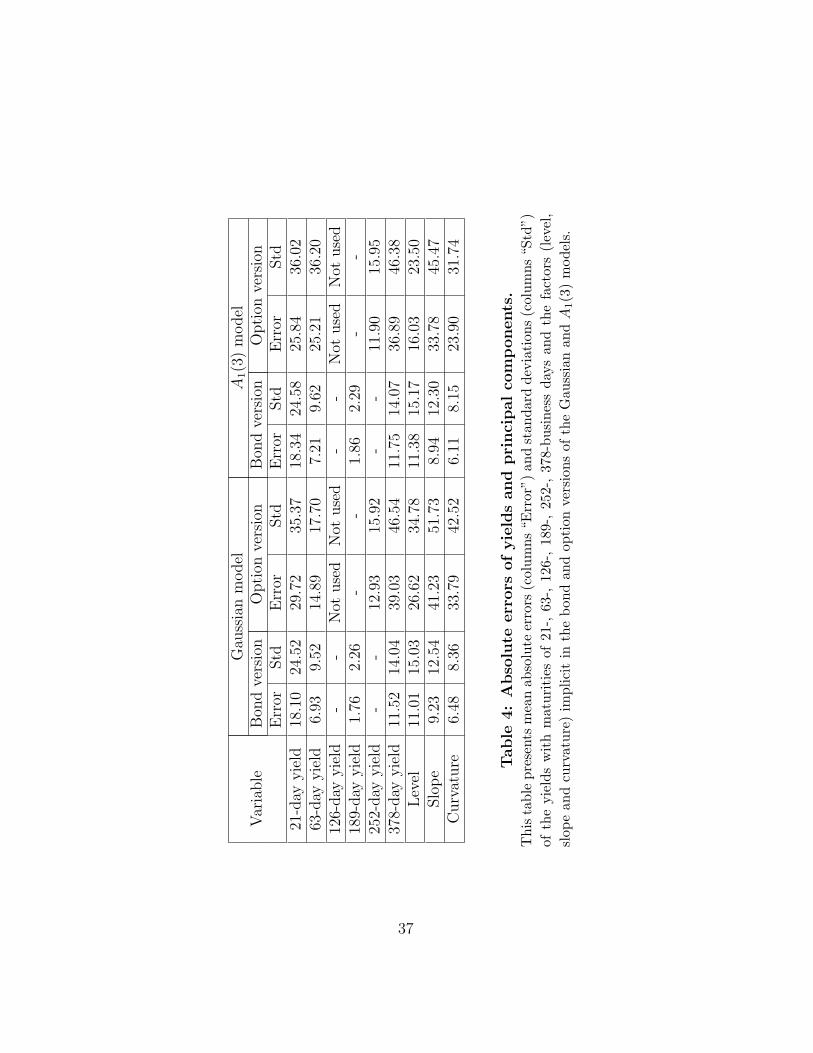
Table 4 presents the mean absolute errors of the yields and principal compo-nents (level, slope and curvature) in both versions of the Gaussian and A1(3)

14We also tested optimization including this parameter, but the results had higher stan-dard errors for a considerable fraction of the parameter vector.

14

models15.For the bond version of the Gaussain model, the mean absolute error

of zero-coupon bond yields with maturities of 21, 63, 189 and 378 businessdays are, respectively, 18.10 bps, 6.93 bps, 1.76 bps and 11.52 bps16. Stan-dard deviations of these errors, which provide a metric for their time seriesvariability, are 24.52 bps, 9.52 bps, 2.26 bps and 14.07 bps. For the optionversion, the mean absolute error of bonds yields with maturities of 21, 63, 252and 378 business days are, respectively, 29.72 bps, 14.89 bps, 12.93 bps and39.03 bps, with standard deviations of 35.37 bps, 17.70 bps, 15.92 bps and46.54 bps. The absolute errors of the principal components are also greaterin the option version, as expected. Figure 2 shows the average observed andmodel implied term structures of interest rates for zero-coupon bonds in eachestimated version of the Gaussian model. It is clear from this figure that onthe pricing of bonds, the bond version outperforms the option version17.

The A1(3) model presents very similar pricing errors as the Gaussianmodel, in both versions. For the bond version, the mean absolute error ofzero-coupon bond yields with maturities of 21, 63, 189 and 378 business daysare respectively 18.34 bps, 7.21 bps, 1.86 bps and 11.75 bps, with valuesfor all maturities approximately 0.2 bps above the Gaussian model. Thestandard deviations of these errors are respectively 24.58 bps, 9.62 bps, 2.29bps and 14.07 bps, practically equal to their Gaussian counterpart values.For the option version of the A1(3) model, the mean absolute error of yieldswith maturities of 21, 63, 252 and 378 business days are, respectively, 25.84bps, 25.21 bps, 11.90 bps and 36.89 bps, with standard deviations of 36.02bps, 36.20 bps, 15.95 bps, and 46.38 bps. Note that the Gaussian and A1(3)models differ only in the error of the 63-business day yield in the optionversion18.

15In order to estimate the errors of the principal components, we first obtain the timeseries of the principal components using the full database of yields. Next we evaluate theimplied components in each version of the models using the implied yields and the samerotation obtained in the first step.

16Bps stands for basis points. One basis point is equivalent to 0.01%.17Under the bond version, the three dimensional latent vector X, characterizing uncer-

tainty in the economy, is fully inverted from bond data. In contrast, the option versiononly captures the yields of two bonds without errors, because the third instrument pricedwithout error is an at-the-money option.

18Probably because the option 95-business day maturity might be affecting the CIRprocess, asymmetrically driving volatility in the A1(3) model (when compared to theGaussian model), slightly distorting the pricing of bonds with maturities close to the

15

Whatever the model used, the option versions consistently price yieldsand principal components worse. Although in the option versions we usefewer bond yields in the estimation procedure, the larger errors suggest thata four-factor affine model would be more appropriate, as pointed out byJoslin (2007).

5.1 Term Structure Movements and Bond Risk Pre-miums

Figure 3 presents the loadings of the three dynamic factors under each versionof the Gaussian model (solid lines correspond to the bond version, dotted linesto the option version). The level factor19 presents loadings indistinguishableacross versions. However, slope and curvature factors are clearly different.They both have higher curvatures in the option version, suggesting thatoption investors tend to react faster (than bond investors) to news that affectthe term structure of bond risk premiums in an asymmetric way20. Similarly,Figure 4 presents the loadings of the three dynamic factors in each version ofthe A1(3) model. Note the similarity between Figures 3 and 4, indicating thatthe modification in the shape of term structure dynamic factors when Asianoptions are included in the estimation process affects the Gaussian modeland the A1(3) model in closely related ways. In the A1(3) model the meanreversion rate of the curvature factor is slightly less affected when options areincluded. In fact, while in the Gaussian model the mean reversion rate of thecurvature factor increases from 6.34 (bond version) to 37.63 (option version),in the A1(3) model it increases from 6.84 to 15.87. Figure 5 presents thestate variables driving each term structure movement, for the two versions ofthe Gaussian model21. Note that the time series of the slope and curvaturefactors, in the option version, have spikes that are consistent with fast meanreverting variables22.

option.19It is the one with slowest mean reversion speeds and responsible for explaining most

of the variation in yields.20Note that a shock in the level factor affects the risk premium term structure symmet-

rically21The average value of the short-rate (φ0) should be added to the level state variable in

order to obtain the level factor.22Results for the time series of dynamic factor are very similar under the A1(3) model,

and are available upon request.

16

An important point related to the modification of term structure move-ments is to understand the implications for investors’ interpretation of riskswhen options are or not included in the estimation process. This can beaddressed in at least two ways: by observing the time series of the model’simplied bond risk premiums and contrasting across versions, or by directlyobserving bond risk premium decomposition as a combination of term struc-ture movements, in each version.

Figure 6 presents graphs of the term structures of the instantaneousbond risk premium (measured by (10)) at different instants, for the Gaus-sian model. Note that the cross section of premiums is very distinct acrossversions, and in particular the longer the maturity the larger is the differ-ence between the risk premium implied by each version. In addition, in theoption version, the term structure of risk premiums is better approximatedby a linear function, and the risk premiums are in general lower. The timeseries behavior of the premiums can be better observed in Figure 7, whichpresents the evolution of the instantaneous risk premium for the 1-year bond,in the two versions. During the period from September 2003 to December2004, the premium is significantly higher under the bond version. That wasa period when interest rates were consistently being lowered by the CentralBank of Brazil. In this context the smaller premium (under the option ver-sion) indicates the possibility of inertia by bond investors in re-estimatingtheir expectations of the long-term behavior of interest rates, as opposed toa faster reaction of option market players.

The risk premium decomposition across movements of the term struc-ture provides a direct way of identifying the shifts in importance of fac-tors when options are included in the estimation process. From (10), itis clear that the risk premium is a linear combination of the state variables:z(t, t+τ) = a1(τ)X1

t +a2(τ)X2t +a3(τ)X3

t . Figure 8 presents, for the Gaussianmodel, the term structure of risk premiums decomposed for each maturityamong the three movements: level, slope and curvature. Solid lines repre-sent the bond version and dashed lines the option version. For each fixedmaturity, the sum of the absolute weights on the three movements is 100%.The decomposition presents a clearly distinct pattern for maturities shorterand longer than 0.5 year, in both versions. For instance, in the bond version,the curvature factor explains more than 70% of the premium for short ma-turities while curvature and slope together explain the premium for longermaturities. In the option version the level factor explains most of the pre-mium for longer maturities while it shares this role with the curvature factor

17

for shorter maturities. In both versions the slope contributes negatively tothe risk premium decomposition. In general, the risk premium is more sen-sitive to the curvature and slope factors in the bond version, and to the leveland curvature factors in the option version. By contrasting factor loadingsand risk premiums, it is possible to identify that the use of options dataprovides less persistent slope and curvature movements, but prices the mostpersistent factor (level). On the other hand, when only bonds are used inthe estimation process, secondary movements (slope and curvature) are morepersistent, but are priced instead of the level movement (still the most persis-tent factor). The results suggest that in the Brazilian fixed income market,options investors are more concerned with monetary policy through interestrate levels, while bond investors are more concerned with the volatility ofinterest rates through curvature and slope (see Litterman et al., 1991).

The corresponding risk premium decomposition in the A1(3) model ispresented in Figure 9. Similarly to the Gaussian model, when options areincluded in the estimation the importance of the level factor in the riskpremium decomposition increases, while the importance of the curvaturefactor decreases. However, the two models disagree on how to price theslope factor. While under the Gaussian model the slope has less influenceon the risk premium when options are included, in the A1(3) model theopposite appears to happen. This might be a consequence of stochasticvolatility in the A1(3) model, driven by the level factor, generating tensionbetween first and second conditional moments. This has been previouslyobserved in the literature on affine dynamic models (see Duffee, 2002 andDuarte, 2004). In any case, we are not advocating that the changes whenAsian options are included in the estimation process should be robust tochanges in the dynamic term structure model chosen. The interesting pointis that both Gaussian and A1(3) models appear to agree on enough pointsto allow a fixed income manager to safely consider implementing the simplerGaussian model (instead of A1(3)) to extract information on shapes and riskpremium structure of term structure movements in joint bond/interest rateAsian option markets.

5.2 Pricing and Hedging Options

The goal of the next exercise is to understand how useful the inclusion ofoptions can be in the estimation process of the dynamic model when pricingand hedging options. Since in the option version an at-the-money option

18

is used to invert the state vector, this exercise is only interesting if out-of-sample options are adopted. For this reason, we use the database of the mostliquid IDI call options when comparing pricing performances across versions.

Figure 10 presents the observed option prices versus those estimated bythe model. The points represent the bond version and x’s the option ver-sion, in the Gaussian model. For modeling purposes, an ideal relation wouldbe a 45 degree line passing through the origin (solid line in Figure 10). Inthe bond version, a linear regression of observed prices depending on modelprices, produces an R2 = 97.5%, an angular coefficient of 1.0423 (p-value< 0.01) and a linear coefficient of 86.83 (p-value < 0.01). The high R2 indi-cates that the option prices obtained in the bond version correctly capturethe time series variability of observed option prices (high correlation). How-ever, the high value of the linear coefficient implies that the bond versionconsistently underestimates option prices. The underestimation of optionprices is confirmed by Figure 11, which shows the relative error defined bymodel price minus observed price, divided by observed price. Note how in thebond version it is smaller than zero most of the time. The absolute relativepricing error has an average of 17.53%23.

When the same regression is performed for the option version, the R2 isslightly lower, at 97.2%, probably due to some mispricing of options withprices in the range [1500, 3000] (see Figure 10). On the other hand, boththe angular coefficient of 1.0121 (p-value < 0.01) and the linear coefficient of11.67 (p-value = 0.14) are closer to ideal values. The smaller linear coefficientindicates that when options are included in the estimation process, they helpthe dynamic model to better capture the level of option prices. The dottedline in Figure 11 shows the relative pricing error for the option version. Notethat it clearly outperforms the bond version, except for the end of the sampleperiod when it overestimates option prices. It achieves an average absolutevalue of 10.75%, a 40% improvement over the bond version.

The next step implements a dynamic delta-hedging strategy on the fixed-maturity at-the-money IDI call option24. Note that if the hedging is effective,variations in the hedging portfolio should approximately offset variations inthe option price. The correlation coefficients between these variations are

23For comparison purposes, see Jagannathan et al. (2003), who price U.S. caps applyinga three-factor CIR model estimated with U.S. Libor and swap data.

24In the hedging analysis we adopted a fixed-maturity, fixed-moneyness option. Other-wise changes in prices would reflect not only the price dynamics but also changes in thetype of the option.

19

5.10% and 94.74% for the bond and option versions respectively, suggestingthat the option-based version is much more efficient when hedging. In fact,one could expect with no surprises that the option version would be ableto hedge well since the at-the-money option is inverted to extract the statevector. In this sense, the hedging error for the option model is essentially asecond-order error not captured by the delta-hedging procedure. However,the result of interest is the comparison of dynamic hedging weights acrossversions. Figure 12 depicts the number of units in the hedging portfolioinvested in each state variable. Observe that in both versions of the model theoption is more sensitive to the level factor and less sensitive to the curvaturefactor, and in particular under the option version, the allocations to bothlevel and slope factors are much more volatile. This high volatility of theallocations reflects the fact that at-the-money options are highly sensitive tochanges in their underlying assets, which in this case are interest rates.

6 Conclusion

Asian options are important over-the-counter instruments that are very valu-able hedging resources. To understand how these options affect correspond-ing bond markets, we used the technology of affine processes to implementdifferent dynamic models including Asian options in the estimation process.In particular, with the use of analytical formulas for bonds and Asian op-tions, two versions of a dynamic multi-factor Gaussian model were estimated,one including only bond data (bond version) and the other combining bondsand interest rate Asian option data (option version). The main interest wasto verify if and how Asian options change the loadings, risk premium andhedging structures of dynamic term structure factors.

We found that interest rate Asian options bring information that primar-ily affects the speed of mean reversion of the slope and curvature of the yieldcurve, and that strongly affects the decomposition of bond risk premiums.In addition, when delta-hedging an at-the-money option, both implementedversions of the Gaussian model gave small importance to the curvature fac-tor, while the option version presented much more volatile weights on slopeand level factors. These seem to be necessary to capture the dynamics ofoption prices.

We also implemented a model generating stochastic volatility for interestrates to verify the validity of the results obtained with the Gaussian model.

20

The stochastic volatility model obtained very similar results (to the Gaussianmodel) regarding the effects of Asian options on the loadings of term struc-ture movements, and partially confirmed the results about the way optionschange the bond risk premium structure. Our results complement theoreticalstudies on the pricing of interest rate Asian options, because we pioneeredimplementations of dynamic models that include these options in the esti-mation process. They should be useful for portfolio and risk managementpurposes as simple and effective tools for pricing and hedging fixed incomeinstruments with the use of interest rate Asian options.

21

Appendix A

Proof. Lemma 1By Ito’s rule, for each t < T the unique strong solution of (3) is25

X iT = X i

te−κi(T−t) +

N∑j=1

ρij

∫ T

t

e−κi(T−s)dW js , i = 1, . . . , N.

Then

rT = φ0 +N∑i=1

(X ite−κi(T−t) +

N∑j=1

ρij

∫ T

t

e−κi(T−s)dW js

).

Stochastic integration by parts implies that∫ T

t

X iudu =

∫ T

t

(T − u) dX iu + (T − t)X i

t . (22)

By definition of X, the integral in the right-hand side can be written as∫ T

t

(T − u) dX iu = −κi

∫ T

t

(T − u)X iudu+

N∑j=1

ρij

∫ T

t

(T − u) dW ju .

Note also that∫ Tt

(T − u)X iudu =

= X it

∫ Tt

(T − u) e−κi(u−t)du+∑N

j=1 ρij∫ Tt

(T − u)∫ ut

e−κi(u−s)dW js du.

Calculating separately the last two integrals, the following result holds∫ T

t

(T − u) e−κi(u−t)du =

(T − tκi

+e−κi(u−t) − 1

κ2i

)25In this appendix we drop the superscript Q and denote the N -dimensional Brownian

motion WQ simply by W .

22

and, again by integration by parts,∫ Tt

(T − u)∫ ut

e−κi(u−s)dW js du =

=∫ Tt

(∫ ut

eκisdW js

)du(∫ u

t(T − v) e−κivdv

)=

=(∫ T

teκiudW j

u

)(∫ Tt

(T − v) e−κivdv)−

−∫ Tt

(∫ ut

(T − v) e−κivdv)

eκiudW ju =

=∫ Tt

(∫ Tu

(T − v) e−κivdv)

eκiudW ju =

1κi

∫ Tt

(T − u+ e−κi(T−u)−1

κi

)dW j

u .

Substituting the previous terms in (22), the following result holds∫ TtX iudu = (T − t)X i

t−

−κi[X it

(T−tκi

+ e−κi(T−t)−1κ2i

)+∑N

j=1ρijκi

∫ Tt

(T − u+ e−κi(T−u)−1

κi

)dW j

u

]+

+∑N

j=1 ρij∫ Tt

(T − u) dW ju =

= − e−κi(T−u)−1κi

X it +∑N

j=1 ρij∫ Tt− e−κi(T−u)−1

κidW j

u =

= 1−e−κi(T−u)

κiX it + 1

κi

∑Nj=1 ρij

∫ Tt

(1− e−κi(T−u)

)dW j

u ,

that is,∫ T

t

X iudu =

1− e−κi(T−u)

κiX it +

1

κi

N∑j=1

ρij

∫ T

t

(1− e−κi(T−u)

)dW j

u . (23)

Then y (t, T ) = φ0 (T − t) +∑N

i=1

∫ TtX iudu conditional on Ft is normally

distributed (see Duffie, 2001) with mean

M(t, T ) = φ0 (T − t) +N∑i=1

1− e−κi(T−t)

κiX it , (24)

23

where the fact that the stochastic integral in (23) is a martingale was used.The variance of y(t, T )|Ft is

V (t, T ) = varQ

[N∑i=1

Yiκi|Ft

], (25)

where Yi =∑N

j=1 ρij∫ Tt

(1− e−κi(T−u)

)dW j

u . Then

V (t, T ) =N∑i=1

varQ (Yi|Ft)κ2i

+ 2N∑i=1

∑k>i

covQ (Yi, Yk|Ft)κiκk

.

Using Ito’s isometry

V (t, T ) =∑N

i=11κ2i

∑Nj=1 ρ

2ij

∫ Tt

(1− e−κi(T−u)

)2du+

+2∑N

i=1

∑k>i

1κiκk

∑Nj=1 ρijρkj

∫ Tt

(1− e−κi(T−u)

) (1− e−κk(T−u)

)du.

(26)At this point, simple integration produces

V (t, T ) =∑N

i=11κ2i

(τ + 2

κie−κiτ − 1

2κie−2κiτ − 3

2κi

)∑Nj=1 ρ

2ij+

+2∑N

i=1

∑k>i

1κiκk

(τ + e−κiτ−1

κi+ e−κkτ−1

κk− e−(κi+κk)τ−1

κi+κk

)∑Nj=1 ρijρkj,

(27)where τ = T − t.

Proof. Lemma 2The martingale condition for bond prices (Duffie, 2001) gives:

P (t, T ) = EQ[e−∫ Tt rudu|Ft

]= EQ [e−y(t,T )|Ft

]. (28)

Now the normality of variable y(t, T )|Ft (Lemma 1), and a simple propertyof the mean of log-normal distributions complete the proof.

Proof. Lemma 3By Equation (11) the proof consists of a simple calculation of the expectation

24

EQ [max (IDIt −Ke−y, 0) |Ft].

c (t, T ) = EQ [max (IDIt −Ke−y, 0) |Ft] =

=∫∞−∞

1√2πV (t,T )

max (IDIt −Ke−y, 0) e−(y−M(t,T ))2

2V (t,T ) dy =

=∫∞

log(K/IDIt)1√

2πV (t,T )(IDIt −Ke−y) e−

(y−M(t,T ))2

2V (t,T ) dy.

(29)

Making the substitution z = y−M(t,T )√V (t,T )

the following result holds:

c (t, T ) =∫∞−d

1√2π

(IDIt −Ke−z

√V (t,T )−M(t,T )

)e−

12z2dz =

= IDTt∫ d−∞

1√2π

e−12z2dz −K

∫∞−d

1√2π

e−z√V (t,T )−M(t,T )− 1

2z2dz =

= IDItΦ (d)−Ke−M(t,T )+V (t,T )

2

∫∞−d

1√2π

e− 1

2

(z+√V (t,T )

)2

dz.

(30)

where d is given by Equation (13). Making a new substitution v = z +√V (t, T ) and using Lemma 2 results in (12).

25

Appendix B

6.1 The Stochastic Volatility Model (A1(3))

We implement a version of an A1(3) model as a robustness check for theresults obtained with the Gaussian model. An A1(3) model is characterizedby the presence of three state variables with one of the them driving theconditional volatility of the short-term rate (Dai and Singleton, 2000). OurA1(3) model is a particular form of a more general one, where the short-termrate is the sum of one independent CIR process (see Cox et al., 1985) withtwo Gaussian processes:

rt = φ0 +Xt + Yt + Zt, (31)

with:

dXt = κX(θ −Xt)dt+ ρX√XtdW

QX(t), (32)

dY Zt =

[dYtdZt

]= −

[ηY 00 ηZ

] [YtZt

]dt+

[ρY 0ρY Z ρZ

] [dWQ

Y (t)

dWQZ (t)

]

= ηY Ztdt+ ρdWQY Z(t), (33)

where WQX , WQ

Y and WQZ are independent Brownian motions under the pricing

measure Q, and where we use the following short notation:

dY Zt =

[dYtdZt

]and dWQ

Y Z(t) =

[dWQ

Y (t)

dWQZ (t)

].

The transition from the pricing measure Q to the objective probabilitymeasure P is given by the extended affine market prices of risks by Cheriditoet al. (2006)26:

dWQX(t) = dW P

X(t) +1√Xt

(λX0 + λX1 Xt

)dt (34)

26In the Gaussian model, this market price of risk coincides with the essentially affinemarket price of risk (Duffee, 2002), indicating that both models (Gaussian and A1(3)) areimplemented with the most general market prices that maintain affine dynamics underboth risk neutral and objective measures.

26

anddWQ

Y Z(t) = dW PY Z(t) +

(λY Z0 + λY Z1 Y Zt

)dt, (35)

where λX0 and λX1 are real numbers, λY Z0 is a vector in R2, and λY Z1 is a 2× 2matrix.

By the independence of the CIR process, it follows directly from theresults of Section 3 and from Brigo and Mercurio (2001) that the time t priceof a zero-coupon bond maturing at time T is given by (τ = T − t):

P (t, T ) = eA(τ)+BX(τ)Xt+BY (τ)Yt+BZ(τ)Zt , (36)

where

A(τ) = −φ0τ +2κXθ

ρXln

(2γe

κX+γ

2

2γ + (κX + γ)(eτγ − 1)

)+VY Z(t, T )

2,

BX(τ) = − 2(eτγ − 1)

2γ + (κX + γ)(eτγ − 1),

BY (τ) = −1− eηY τ

ηY,

and

BZ(τ) = −1− eηZτ

ηZ,

with γ =√κ2X + 2ρ2

X and VY Z given by (6), with N = 2 and κ = η.According to the explanation in Section 3, the pricing of IDI options

demands knowledge of the distribution of y(t, T ) conditional on the informa-tion available at time t. If rt is a Gaussian process, then y|Ft is normallydistributed. However, in the A1(3) case there is not a simple numerical pro-cedure to calculate probabilities related to y. Nevertheless, the moment oforder m of e−y(t,T ) can be calculated, since it is the price of a bond whenthe short-term rate is m× rt. Therefore we can use an Edgeworth expansiontechnique to obtain IDI Asian option prices (see Collin-Dufresne and Gold-stein, 2002b, for its use on swaptions pricing). In the next lines we describehow to apply this technique in our A1(3) version. Using the forward measureapproach (Geman et al., 1995), the price of the IDI option is given by:

c(t, T ) = IDItPQt (e−y < IDIt/K)−KP (t, T )PTt (e−y < IDIt/K),

27

where Pt denotes probabilities conditional on Ft and the superscript T rep-resents the forward measure.

The probabilities in the right-hand side of the above equation can becalculated using the Edgeworth expansion. The Edgeworth expansion isbasically an expansion of a distribution around the normal distribution. Fol-lowing Collin-Dufresne and Goldstein (2002b), we expand up to the seventhorder. In this case, the probabilities Pt are equal to 1 −

∑7j=0 αjβj, where

the coefficients αj are ratios of polynomials of order 7 in the moments ofe−y(t,T ) and βj are simple functions of the cumulative normal function andthe first two moments of e−y(t,T )27. The moments of e−y(t,T ) under both therisk neutral measure Q and the forward measure are obtained as describedin the previous paragraph. However, the computation of these momentsunder the forward measure are slightly more difficult, since rt under the for-ward measure T follows a Hull and White (1990) process with time-varyingparameters. Therefore, we do not have closed-form expressions for bonds,and adopt the Runge-Kutta method to solve numerically the coupled pairof differential equations satisfied by terms A and B appearing in the bondexpression.

27Collin-Dufresne and Goldstein (2002b) provide the precise expressions for the coeffi-cients αj and βj .

28

Appendix C - Estimation Procedure

Gaussian Model

In this work, in the Gaussian model the maximum likelihood estimation pro-cedure described in Chen and Scott (1993) is extended to deal with options28.The following bond yields are observed along H different days: rbt(1/252),rbt(21/252), rbt(63/252), rbt(126/252), rbt(189/252), rbt(1) and rbt(1.5)29.Let rb represent the H × 7 matrix containing the yields for all H days. Inaddition, the price cst for an at-the-money call with time to maturity 95/252years is observed during the same H days. Let cs be the vector of length Hthat represents these call prices. The ID bonds and the at-the-money IDIcall are called reference market instruments. Denote by rmi = [rb, cs] theH × 8 matrix containing the yields and the price of these reference marketinstruments. Assume that the model parameters are represented by vectorφ and a time unit equal to ∆t. Finally, let gi(Xt; t, φ) be the function thatmaps reference market instrument i into state variables.

Since three factors are adopted to estimate the model, is assumed thatreference market instruments, say i1, i2 and i3, are observed without error.For each fixed t, the state vector is obtained through the solution of thefollowing system:

gi1(Xt; t, φ) = rmi(t, i1)

gi2(Xt; t, φ) = rmi(t, i2)

gi3(Xt; t, φ) = rmi(t, i3).

(37)

Reference market instruments i4, i5, i6, i7 and i8, are assumed to be observedwith Gaussian uncorrelated errors ut:

rmi(t,[i4 i5 i6 i7 i8

])− ut =[

gi4(Xt; t, φ) gi5(Xt; t, φ) gi6(Xt; t, φ) gi7(Xt; t, φ) gi8(Xt; t, φ)].(38)

28For the estimation of more general dynamic term structure models based on jointbond-option data, see for instance, Umantsev (2001), Han (2007) and Almeida et al.(2006), among others.

29rbt(τ) stands for the time t yield of a bond with time to maturity τ .

29

The log-likelihood function can be written as

L(φ, rb) =∑H

t=2 log p(Xt|Xt−1;φ)−

−∑H

t=2 log |Jact| − H−12

log |Ω| − 12

∑Ht=2 u

′tΩ−1ut,

(39)

where:

1. Jact =

∂gi1 (Xt;t,φ)

∂Xt

∂gi2 (Xt;t,φ)

∂Xt

∂gi3 (Xt;t,φ)

∂Xt

is the Jacobian matrix of the transformation

defined by (37);

2. Ω represents the covariance matrix for ut, estimated using the samplecovariance matrix of the ut’s implied by the extracted state vector;

3. p(Xt|Xt−1;φ) is the transition probability from Xt−1 to Xt under theobjective probability measure P.

The final objective of this procedure is to estimate vector φ, which max-imizes function L(φ, rb). In order to avoid possible local minima, severaldifferent starting parameter vectors are tested and for each on a search forthe optimal point is performed, using Nelder-Mead Simplex algorithm fornonlinear optimization and gradient-based optimization methods.

A1(3) Model

In the A1(3) model, we also follow a procedure similar to Chen and Scott(1993) but instead of maximum likelihood, we perfom a quasi maximumlikelihood (QML) estimation. Although the transition probabilities under theA1(3) model is the product of a non-central chi-square density and a Gaussiandensity, for stability purposes we decided to implement QML, since we haveanalytical formulas for the first two conditional moments of the state vectorin any affine model. Other than applying QML, the rest of the estimationprocedure is precisely as described above for the Gaussian model.

30

References

[1] Ahn D.H., R. Dittmar, and R. Gallant (2002). Quadratic Term StructureModels: Theory and Evidence. Review of Financial Studies, 15, 1, 243-288.

[2] Almeida C., J. Graveline, and S. Joslin (2006). Do Fixed Income OptionsContain Information About Excess Returns?, Working Paper, StanfordGraduate School of Business.

[3] Almeida C. and J. Vicente (2009). Identifying Volatility Risk Premiafrom Fixed Income Asian Options. Journal of Banking and Finance, 33,652-661.

[4] Bakshi G. and D. Madan (1999). A Unified Treatment of Average-Rate Contingent Claims with Applications. Working Paper, Universityof Maryland.

[5] Bikbov R. and M. Chernov (2005). Term Structure and Volatility:Lessons from the Eurodollar Markets. Working Paper, Division of Fi-nance and Economics, Columbia University.

[6] Brace A. (2008). Engineering BGM, Chapman & Hall/Crc FinancialMathematics Series.

[7] Brigo D. and F. Mercurio (2001). Interest Rate Models: Theory andPractice, Springer Verlag.

[8] Chacko G. and S. Das (2002). Pricing Interest Rate Derivatives: A Gen-eral Approach. Review of Financial Studies, 15, 1, 195-241.

[9] Chen R.R. and L. Scott (1993). Maximum Likelihood Estimation for aMultifactor Equilibrium Model of the Term Structure of Interest Rates.Journal of Fixed Income, 3, 14-31.

[10] Cheridito P., D. Filipovic, and R. Kimmel (2007). Market Price of RiskSpecifications for Affine Models: Theory and Evidence. Journal of Fi-nancial Economics, 83, 1, 123-170.

[11] Cheuk T.H.F. and T.C.F. Vorst (1999). Average Interest Rate Caps.Computational Economics, 14, 183-196.

31

[12] Collin Dufresne P. and R.S. Goldstein (2002a). Do Bonds Span theFixed Income Markets? Theory and Evidence for Unspanned StochasticVolatility. Journal of Finance, LVII, 4, 1685-1730.

[13] Collin Dufresne P. and R.S. Goldstein (2002b). Pricing SwaptionsWithin an Affine Framework. Journal of Derivatives, Vol. 10, 1.

[14] Cox J. C., J.E. Ingersoll and S.A. Ross (1985). A Theory of the TermStructure of Interest Rates. Econometrica, 53, 385-407.

[15] Dai Q. and K. Singleton (2000). Specification Analysis of Affine TermStructure Models. Journal of Finance, LV, 5, 1943-1977.

[16] Dassios A. and J. Nagaradjasarma (2003). Pricing Asian Options OnInterest Rates in the CIR Model. Working Paper, Department of Statis-tics, London School of Economics.

[17] Davidson R. and J.G. MacKinnon (1993). Estimation and Inference inEconometrics. Oxford University Press.

[18] Duarte J. (2004). Evaluating an Alternative Risk Preference in AffineTerm Strcuture Models. Review of Financial Studies, 17, 2, 370-404.

[19] Duffee G. R. (2002). Term Premia and Interest Rates Forecasts in AffineModels. Journal of Finance, 57, 405-443.

[20] Duffie D. (2001). Dynamic Asset Pricing Theory, Princeton UniversityPress.

[21] Duffie D. and R. Kan (1996). A Yield Factor Model of Interest Rates.Mathematical Finance, Vol. 6, 4, 379-406.

[22] Geman H., N. El Karoui, and J.-C. Rochet (1995). Changes of Nu-meraire, Changes of Probability Measure and Option Pricing. Journalof Applied Probability, 32, 2, 443-458.

[23] Geman H. and M. Yor (1993). Bessel Processes, Asian Options andPerpetuities. Mathematical Finance, 3, 349-375.

[24] Han B. (2007). Stochastic Volatility and Correlations of Bond Yields.Journal of Finance, vol LXII, 3, 1491-1523.

32

[25] Hull J. And A. White (1990). Pricing Interest Rate Derivatives Securi-ties. Review of Financial Studies, 3, 4, 573-592.

[26] Jagannathan R., A. Kaplin, and S. Sun (2003). An Evaluation of Multi-factor CIR Models using LIBOR, Swap Rates, and Cap and SwaptionsPrices. Journal of Econometrics, 116, 113-146.

[27] Joslin S. (2007). Pricing and Hedging Volatility Risk in Fixed IncomeMarkets. Working Paper, Sloan School of Management, MIT.

[28] Leblanc B. and O. Scaillet (1998). Path Dependent Options on Yields inthe Affine Term Structure Model. Finance and Stochastics, 2, 349-367.

[29] Li H. and F. Zhao (2006). Unspanned Stochastic Volatility: Evidencefrom Hedging Interest Rates Derivatives. Journal of Finance, 61, 1,341-378.

[30] Litterman R., J.A. Scheinkman, and L. Weiss (1991). Volatility and theYield Curve. Journal of Fixed Income, 1, 49-53.

[31] Longstaff F.A. (1995). Hedging Interest Rate Risk with Options on Av-erage Interest Rates. Journal of Fixed Income, March, 37-45.

[32] Pan, J. and K. Singleton (2008). Default and recovery implicit in theterm structure of sovereign CDS spreads. Journal of Finance, 63, 5,2345-2384.

[33] Umantsev L. (2001). Econometric Analysis of European Libor-BasedOptions within Affine Term Structure Models. PhD Thesis, Departmentof Management Science and Engineering, Stanford University.

[34] Vasicek O.A. (1977). An Equilibrium Characterization of the TermStructure. Journal of Financial Economics, 5, 177-188.

33

OptionAverageprice

Pricevolatility

Averagemoneyness

Averagematurity(business days)

Most liquid 989.22 833.37 0.9951 105.01At-the-money 281.30 91.16 1 95

Table 1: Descriptive statistics of options.This table presents descriptive statistics of two different options databases.The first is composed of an at-the-money IDI call with maturity of 95business days and moneyness of one. The second is composed of the mostliquid IDI call on each day. The sample size is 748 business days, coveringthe period from January 2003 until December 2005.

Figure 1: Time series of Brazilian bonds yields.This figure contains the time series of Brazilian bond yields extracted fromID-futures with maturities of 1 month (21 business day), 6 months (126business days) and 12 months (252 business days) between January 2003and December 2005.

34

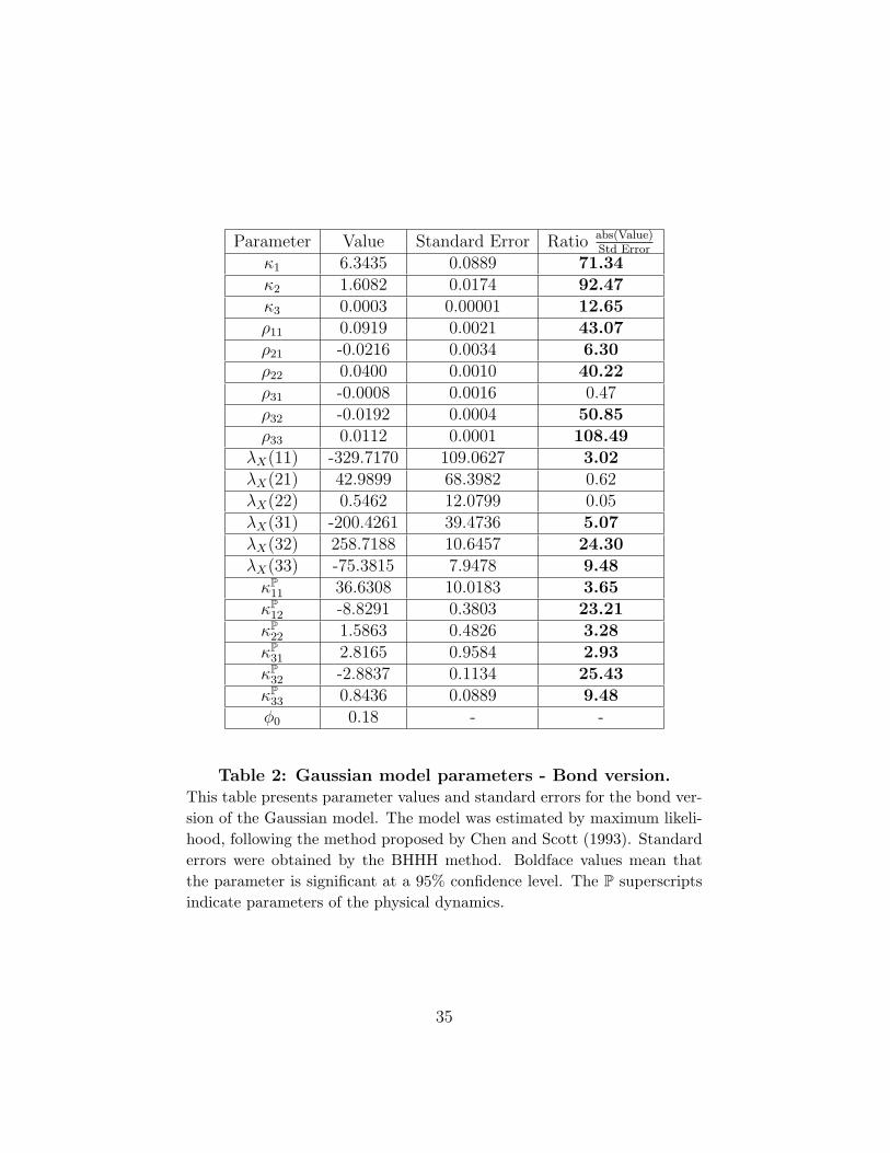
Parameter Value Standard Error Ratio abs(Value)Std Error

κ1 6.3435 0.0889 71.34κ2 1.6082 0.0174 92.47κ3 0.0003 0.00001 12.65ρ11 0.0919 0.0021 43.07ρ21 -0.0216 0.0034 6.30ρ22 0.0400 0.0010 40.22ρ31 -0.0008 0.0016 0.47ρ32 -0.0192 0.0004 50.85ρ33 0.0112 0.0001 108.49

λX(11) -329.7170 109.0627 3.02λX(21) 42.9899 68.3982 0.62λX(22) 0.5462 12.0799 0.05λX(31) -200.4261 39.4736 5.07λX(32) 258.7188 10.6457 24.30λX(33) -75.3815 7.9478 9.48κP

11 36.6308 10.0183 3.65κP

12 -8.8291 0.3803 23.21κP

22 1.5863 0.4826 3.28κP

31 2.8165 0.9584 2.93κP

32 -2.8837 0.1134 25.43κP

33 0.8436 0.0889 9.48φ0 0.18 - -

Table 2: Gaussian model parameters - Bond version.This table presents parameter values and standard errors for the bond ver-sion of the Gaussian model. The model was estimated by maximum likeli-hood, following the method proposed by Chen and Scott (1993). Standarderrors were obtained by the BHHH method. Boldface values mean thatthe parameter is significant at a 95% confidence level. The P superscriptsindicate parameters of the physical dynamics.

35

Parameter Value Standard Error Ratio abs(Value)Std Error

κ1 37.6296 10.8910 3.46κ2 3.4565 0.1858 18.60κ3 0.0003 0.00002 16.96ρ11 0.0951 0.0040 23.77ρ21 -0.0415 0.0044 9.41ρ22 0.0729 0.0016 45.45ρ31 -0.0006 0.0017 0.39ρ32 -0.0332 0.0016 20.72ρ33 0.0194 0.0003 69.66

λX(11) -240.0116 129.1894 1.86λX(21) -137.1462 63.9335 2.15λX(22) 0.0376 12.4838 0.00λX(31) -260.0849 84.7153 3.07λX(32) 16.917 26.6624 0.63λX(33) -278.9916 13.1735 21.17κP

11 60.4487 22.8191 2.65κP

12 0.0354 0.0350 1.01κP

22 3.4538 0.0872 39.60κP

31 0.3261 0.3153 1.03κP

32 -0.3263 0.1294 2.52κP

33 5.4016 2.6102 2.07φ0 0.18 - -

Table 3: Gaussian model parameters - Option version.This table presents parameter values and standard errors for the optionversion of the Gaussian model. The model was estimated by maximumlikelihood following the method proposed by Chen and Scott (1993). Stan-dard errors were obtained by the BHHH method. Boldface values meanthat the parameter is significant at a 95% confidence level. The P super-scripts indicate parameters of the physical dynamics.

36

Var

iable

Gau

ssia

nm

odel

A1(3

)m

odel

Bon

dve

rsio

nO

pti

onve

rsio

nB

ond

vers

ion

Opti

onve

rsio

nE

rror

Std

Err

orStd

Err

orStd

Err

orStd

21-d

ayyie

ld18

.10

24.5

229

.72

35.3

718

.34

24.5

825

.84

36.0

263

-day

yie

ld6.

939.

5214

.89

17.7

07.

219.

6225

.21

36.2

012

6-day

yie

ld-

-N

otuse

dN

otuse

d-

-N

otuse

dN

otuse

d18

9-day

yie

ld1.

762.

26-

-1.

862.

29-

-25

2-day

yie

ld-

-12

.93

15.9

2-

-11

.90

15.9

537

8-day

yie

ld11

.52

14.0

439

.03

46.5

411

.75

14.0

736

.89

46.3

8L

evel

11.0

115

.03

26.6

234

.78

11.3

815

.17

16.0

323

.50

Slo

pe

9.23

12.5

441

.23

51.7

38.

9412

.30

33.7

845

.47

Curv

ature

6.48

8.36

33.7

942

.52

6.11

8.15

23.9

031

.74

Table

4:

Abso

lute

err

ors

ofyie

lds

and

pri

nci

palco

mponents

.T

his

tabl

epr

esen

tsm

ean

abso

lute

erro

rs(c

olum

ns“E

rror

”)an

dst

anda

rdde

viat

ions

(col

umns

“Std

”)of

the

yiel

dsw

ith

mat

urit

ies

of21

-,63

-,12

6-,

189-

,25

2-,

378-

busi

ness

days

and

the

fact

ors

(lev

el,

slop

ean

dcu

rvat

ure)

impl

icit

inth

ebo

ndan

dop

tion

vers

ions

ofth

eG

auss

ian

andA

1(3

)m

odel

s.

37

Figure 2: Average cross-section of yields - Gaussian model.This figure shows the average observed and model-estimated cross-sectionof yields in the bond (solid line) and option (dashed line) versions of theGaussian model. In the bond version, the model is estimated based onlyon the ID-future market, while in the option version information from theIDI call is also included.

38

Figure 3: Loadings of the dynamic factors - Gaussian model.This figure contains the loadings of the three dynamic factors (level, slopeand curvature) in the bond (solid line) and option (dashed line) versionsof the Gaussian model. In the bond version, the model is estimated basedonly on the ID-future market, while in the option version information fromthe IDI call is also included.

39

Figure 4: Loadings of the dynamic factors - A1(3) model.This figure contains the loadings of the three dynamic factors (level, slopeand curvature) in the bond (solid line) and option (dashed line) versions ofthe A1(3) model. In the bond version, the model is estimated based onlyon the ID-future market, while in the option version information from theIDI call is also included.

40

Figure 5: Time series of the state variables - Gaussian model.This figure contains the time series of the state variables in the Gaussianmodel between January 2003 and December 2005. The left-hand panelshows the bond version of the model and the right-hand panel the optionversion. In the bond version, the model is estimated based only on theID-future market while in the option version information from the IDI callis also included.

41

Figure 6: Excess returns - Gaussian model.This figure shows examples of cross-section instantaneous expected excessreturns in the bond (solid line) and option (dashed line) versions of theGaussian model. In the bond version, the model is estimated based onlyon the ID-future market, while in the option version information from theIDI call is also included.

42

Figure 7: 1-year bond excess return - Gaussian model.This figure shows the time series of instantaneous expected excess returnof the 1-year bond for the bond and option versions in the Gaussian model.In the bond version, the model is estimated based only on the ID-futuremarket, while in the option version information from the IDI call is alsoincluded.

43

Figure 8: Bond risk premium decomposition - Gaussianmodel.This figure shows the bond risk premium decomposition for the bond ver-sion (solid line) and option version (dashed line) in the Gaussian model.In the bond version, the model is estimated based only on the ID-futuremarket, while in the option version information from the IDI call is alsoincluded.

44

Figure 9: Bond risk premium decomposition - A1(3) model.This figure shows the bond risk premium decomposition for the bond ver-sion (solid line) and option version (dashed line) in the A1(3) model. In thebond version, the model is estimated based only on the ID-future market,while in the option version information from the IDI call is also included.

45

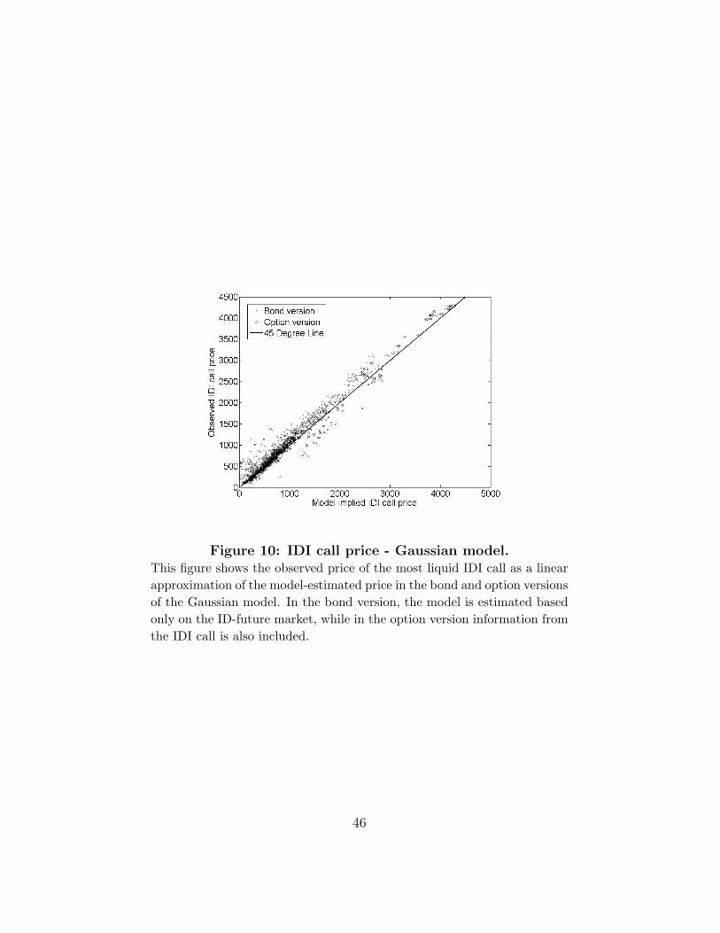
Figure 10: IDI call price - Gaussian model.This figure shows the observed price of the most liquid IDI call as a linearapproximation of the model-estimated price in the bond and option versionsof the Gaussian model. In the bond version, the model is estimated basedonly on the ID-future market, while in the option version information fromthe IDI call is also included.

46

Figure 11: IDI call relative price error - Gaussian model.This figure shows the model relative error ( Model price

Observed price− 1) when pricing

the most liquid IDI call based in parameters estimated in the bond version(solid line) and option version (dotted line) of the Gaussian model. In thebond version, the model is estimated based only on the ID-future market,while in the option version information from the IDI call is also included.

47

Figure 12: Hedging portfolio - Gaussian model.This figure shows the time series of the number of units (qi, i = 1, 2, 3) ofstate variables in the hedging portfolio in the bond (left-hand panel) andoption (right-hand panel) versions of Gaussian model. In the bond version,the model is estimated based only on the ID-future market, while in theoption version information from the IDI call is also included.

48