glimmer-cism 1.7.1 documentation · 2013-06-07 · braries. this section documents how to get...
TRANSCRIPT
Glimmer-CISM 1.7.1 Documentation
Magnus Hagdorn1, Ian Rutt2, Tony Payne3 Felix Hebeler4 and Timothy R. Wylie
May 28, 2013
[email protected]@[email protected]@geo.unizh.ch

ii
Contents
I User Documentation 1
1 User Guide 31.1 Introduction . . . . . . . . . . . . . . . . . . . . . . . . . . . . . . . . . . . . . . . 3
1.1.1 Overview . . . . . . . . . . . . . . . . . . . . . . . . . . . . . . . . . . . . 31.1.2 Climate Drivers . . . . . . . . . . . . . . . . . . . . . . . . . . . . . . . . . 41.1.3 Configuration, I/O and Visualisation . . . . . . . . . . . . . . . . . . . . . 4
1.2 Getting and Installing GLIMMER . . . . . . . . . . . . . . . . . . . . . . . . . . 61.2.1 Prerequisites . . . . . . . . . . . . . . . . . . . . . . . . . . . . . . . . . . 61.2.2 The GLIMMER Directory Structure . . . . . . . . . . . . . . . . . . . . . 61.2.3 Installing a Released Version of GLIMMER . . . . . . . . . . . . . . . . . 71.2.4 Installing from CVS . . . . . . . . . . . . . . . . . . . . . . . . . . . . . . 71.2.5 Profiling . . . . . . . . . . . . . . . . . . . . . . . . . . . . . . . . . . . . . 81.2.6 Restarts . . . . . . . . . . . . . . . . . . . . . . . . . . . . . . . . . . . . . 8
1.3 GLIDE . . . . . . . . . . . . . . . . . . . . . . . . . . . . . . . . . . . . . . . . . 81.3.1 Configuration . . . . . . . . . . . . . . . . . . . . . . . . . . . . . . . . . . 8
1.4 Example Climate Drivers . . . . . . . . . . . . . . . . . . . . . . . . . . . . . . . 151.4.1 EISMINT Driver . . . . . . . . . . . . . . . . . . . . . . . . . . . . . . . . 151.4.2 EIS Driver . . . . . . . . . . . . . . . . . . . . . . . . . . . . . . . . . . . 161.4.3 GLINT driver . . . . . . . . . . . . . . . . . . . . . . . . . . . . . . . . . . 18
1.5 Supplied mass-balance schemes . . . . . . . . . . . . . . . . . . . . . . . . . . . . 221.5.1 Overview . . . . . . . . . . . . . . . . . . . . . . . . . . . . . . . . . . . . 221.5.2 Annual PDD scheme . . . . . . . . . . . . . . . . . . . . . . . . . . . . . . 231.5.3 Daily PDD scheme . . . . . . . . . . . . . . . . . . . . . . . . . . . . . . . 25
2 Tutorial 272.1 Introduction . . . . . . . . . . . . . . . . . . . . . . . . . . . . . . . . . . . . . . . 272.2 EISMINT: using glimmer-example . . . . . . . . . . . . . . . . . . . . . . . . . . 272.3 EIS: using glimmer-tests . . . . . . . . . . . . . . . . . . . . . . . . . . . . . . . 29
2.3.1 A short introduction to the EIS driver parameterisation . . . . . . . . . . 292.4 GLINT: using glint-example . . . . . . . . . . . . . . . . . . . . . . . . . . . . . . 31
II Developer Documentation 33
3 Numerics 353.1 Ice Thickness Evolution . . . . . . . . . . . . . . . . . . . . . . . . . . . . . . . . 35
3.1.1 Numerical Grid . . . . . . . . . . . . . . . . . . . . . . . . . . . . . . . . . 363.1.2 Ice Sheet Equations in σ–Coordinates . . . . . . . . . . . . . . . . . . . . 383.1.3 Calculating the Horizontal Velocity and the Diffusivity . . . . . . . . . . . 393.1.4 Solving the Ice Thickness Evolution Equation . . . . . . . . . . . . . . . . 393.1.5 Calculating Vertical Velocities . . . . . . . . . . . . . . . . . . . . . . . . . 42
iii
iv CONTENTS
3.2 Temperature Solver . . . . . . . . . . . . . . . . . . . . . . . . . . . . . . . . . . . 44
3.2.1 Vertical Diffusion . . . . . . . . . . . . . . . . . . . . . . . . . . . . . . . . 45
3.2.2 Horizontal Advection . . . . . . . . . . . . . . . . . . . . . . . . . . . . . . 45
3.2.3 Heat Generation . . . . . . . . . . . . . . . . . . . . . . . . . . . . . . . . 46
3.2.4 Vertical Advection . . . . . . . . . . . . . . . . . . . . . . . . . . . . . . . 46
3.2.5 Boundary Conditions . . . . . . . . . . . . . . . . . . . . . . . . . . . . . 47
3.2.6 Putting it all together . . . . . . . . . . . . . . . . . . . . . . . . . . . . . 47
3.3 Basal Boundary Condition . . . . . . . . . . . . . . . . . . . . . . . . . . . . . . . 48
3.3.1 Mechanical Boundary Conditions . . . . . . . . . . . . . . . . . . . . . . . 49
3.3.2 Thermal Boundary Conditions . . . . . . . . . . . . . . . . . . . . . . . . 49
3.3.3 Numerical Solution . . . . . . . . . . . . . . . . . . . . . . . . . . . . . . . 51
3.3.4 Basal Hydrology . . . . . . . . . . . . . . . . . . . . . . . . . . . . . . . . 51
3.3.5 Putting It All Together . . . . . . . . . . . . . . . . . . . . . . . . . . . . 51
3.4 Isostatic Adjustment . . . . . . . . . . . . . . . . . . . . . . . . . . . . . . . . . . 53
3.4.1 Calculation of ice-water load . . . . . . . . . . . . . . . . . . . . . . . . . 53
3.4.2 Elastic lithosphere model . . . . . . . . . . . . . . . . . . . . . . . . . . . 54
3.4.3 Relaxing aesthenosphere model . . . . . . . . . . . . . . . . . . . . . . . . 54
4 Developer Guide 55
4.1 Introduction . . . . . . . . . . . . . . . . . . . . . . . . . . . . . . . . . . . . . . . 55
4.2 Introduction to GLIMMER programming techniques . . . . . . . . . . . . . . . . 56
4.2.1 Fortran Modules . . . . . . . . . . . . . . . . . . . . . . . . . . . . . . . . 56
4.2.2 Derived types . . . . . . . . . . . . . . . . . . . . . . . . . . . . . . . . . . 58
4.2.3 Object-orientation with modules and derived types . . . . . . . . . . . . . 58
4.2.4 Example of OOP in Glimmer . . . . . . . . . . . . . . . . . . . . . . . . . 59
4.2.5 Pointers . . . . . . . . . . . . . . . . . . . . . . . . . . . . . . . . . . . . . 60
4.3 GLIMMER structure and design . . . . . . . . . . . . . . . . . . . . . . . . . . . 62
4.3.1 Overview . . . . . . . . . . . . . . . . . . . . . . . . . . . . . . . . . . . . 62
4.3.2 GLIDE structure . . . . . . . . . . . . . . . . . . . . . . . . . . . . . . . . 63
4.3.3 GLINT structure . . . . . . . . . . . . . . . . . . . . . . . . . . . . . . . . 66
4.4 Physics documentation . . . . . . . . . . . . . . . . . . . . . . . . . . . . . . . . . 68
4.4.1 Ice temperature evolution routines . . . . . . . . . . . . . . . . . . . . . . 68
4.5 Configuration File Parser . . . . . . . . . . . . . . . . . . . . . . . . . . . . . . . 70
4.5.1 File Format . . . . . . . . . . . . . . . . . . . . . . . . . . . . . . . . . . . 70
4.5.2 Architecture Overview . . . . . . . . . . . . . . . . . . . . . . . . . . . . . 70
4.5.3 API . . . . . . . . . . . . . . . . . . . . . . . . . . . . . . . . . . . . . . . 71
4.6 netCDF I/O . . . . . . . . . . . . . . . . . . . . . . . . . . . . . . . . . . . . . . . 72
4.6.1 Data Structures . . . . . . . . . . . . . . . . . . . . . . . . . . . . . . . . . 72
4.6.2 The Code Generator . . . . . . . . . . . . . . . . . . . . . . . . . . . . . . 72
4.6.3 Variable Definition File . . . . . . . . . . . . . . . . . . . . . . . . . . . . 72
III Appendix 75
A netCDF Variables 77
A.1 Glide Variables . . . . . . . . . . . . . . . . . . . . . . . . . . . . . . . . . . . . . 77
A.2 EIS Variables . . . . . . . . . . . . . . . . . . . . . . . . . . . . . . . . . . . . . . 79
A.3 GLINT Variables . . . . . . . . . . . . . . . . . . . . . . . . . . . . . . . . . . . . 79
CONTENTS v
B The GLIMMER API 81B.1 GLUM . . . . . . . . . . . . . . . . . . . . . . . . . . . . . . . . . . . . . . . . . . 81
B.1.1 Subroutine open log . . . . . . . . . . . . . . . . . . . . . . . . . . . . . . 81B.1.2 Subroutine ConfigRead . . . . . . . . . . . . . . . . . . . . . . . . . . . . 81B.1.3 Subroutine CheckSections . . . . . . . . . . . . . . . . . . . . . . . . . . 82
B.2 GLIDE . . . . . . . . . . . . . . . . . . . . . . . . . . . . . . . . . . . . . . . . . 82B.2.1 Subroutine glide config . . . . . . . . . . . . . . . . . . . . . . . . . . . 82B.2.2 Subroutine glide initialise . . . . . . . . . . . . . . . . . . . . . . . . 82B.2.3 Subroutine glide nc fillall . . . . . . . . . . . . . . . . . . . . . . . . . 82B.2.4 Subroutine glide tstep p1 . . . . . . . . . . . . . . . . . . . . . . . . . . 83B.2.5 Subroutine glide tstep p2 . . . . . . . . . . . . . . . . . . . . . . . . . . 83B.2.6 Subroutine glide tstep p3 . . . . . . . . . . . . . . . . . . . . . . . . . . 83B.2.7 Subroutine glide finalise . . . . . . . . . . . . . . . . . . . . . . . . . . 84
B.3 GLINT . . . . . . . . . . . . . . . . . . . . . . . . . . . . . . . . . . . . . . . . . 84B.3.1 Subroutine initialise glint . . . . . . . . . . . . . . . . . . . . . . . . 84B.3.2 Subroutine glint . . . . . . . . . . . . . . . . . . . . . . . . . . . . . . . . 85B.3.3 Subroutine end glint . . . . . . . . . . . . . . . . . . . . . . . . . . . . . 87B.3.4 Function glint coverage map . . . . . . . . . . . . . . . . . . . . . . . . 87

vi CONTENTS
Part I
User Documentation
1

Chapter 1
User Guide
1.1 Introduction
GLIMMER1 is a set of libraries, utilities and example climate drivers used to simulate icesheet evolution. At its core, it implements the standard, shallow-ice representation of ice sheetdynamics. This approach to ice sheet modelling is well-established, as are the numerical methodsused. What is innovative about GLIMMER is its design, which is motivated by the desire tocreate an ice modelling system which is easy to interface to a wide variety of climate models,without the user having to have a detailed knowledge of its inner workings. This is achievedby several means, including the provision of a well-defined code interface to the model2, as wellas the adoption of a very modular design. The model is coded almost entirely in standards-complient Fortran 95, and extensive use is made of the advances features of that language.NOTE: Parts of this documentation are known to be out of date and will updatedas part of an upcoming, stand-alone model release. The model options discussed insection 1.3.1 have been updated to be consistent with the version of CISM releasedas part of CESM 1.2.
1.1.1 Overview
GLIMMER consists of several components:
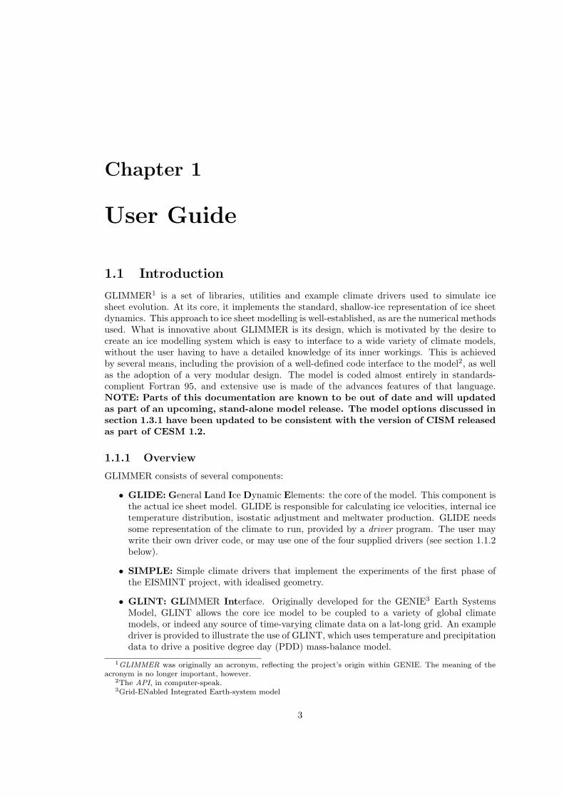
• GLIDE: General Land Ice Dynamic Elements: the core of the model. This component isthe actual ice sheet model. GLIDE is responsible for calculating ice velocities, internal icetemperature distribution, isostatic adjustment and meltwater production. GLIDE needssome representation of the climate to run, provided by a driver program. The user maywrite their own driver code, or may use one of the four supplied drivers (see section 1.1.2below).
• SIMPLE: Simple climate drivers that implement the experiments of the first phase ofthe EISMINT project, with idealised geometry.
• GLINT: GLIMMER Interface. Originally developed for the GENIE3 Earth SystemsModel, GLINT allows the core ice model to be coupled to a variety of global climatemodels, or indeed any source of time-varying climate data on a lat-long grid. An exampledriver is provided to illustrate the use of GLINT, which uses temperature and precipitationdata to drive a positive degree day (PDD) mass-balance model.
1GLIMMER was originally an acronym, reflecting the project’s origin within GENIE. The meaning of theacronym is no longer important, however.
2The API, in computer-speak.3Grid-ENabled Integrated Earth-system model
3
4 CHAPTER 1. USER GUIDE
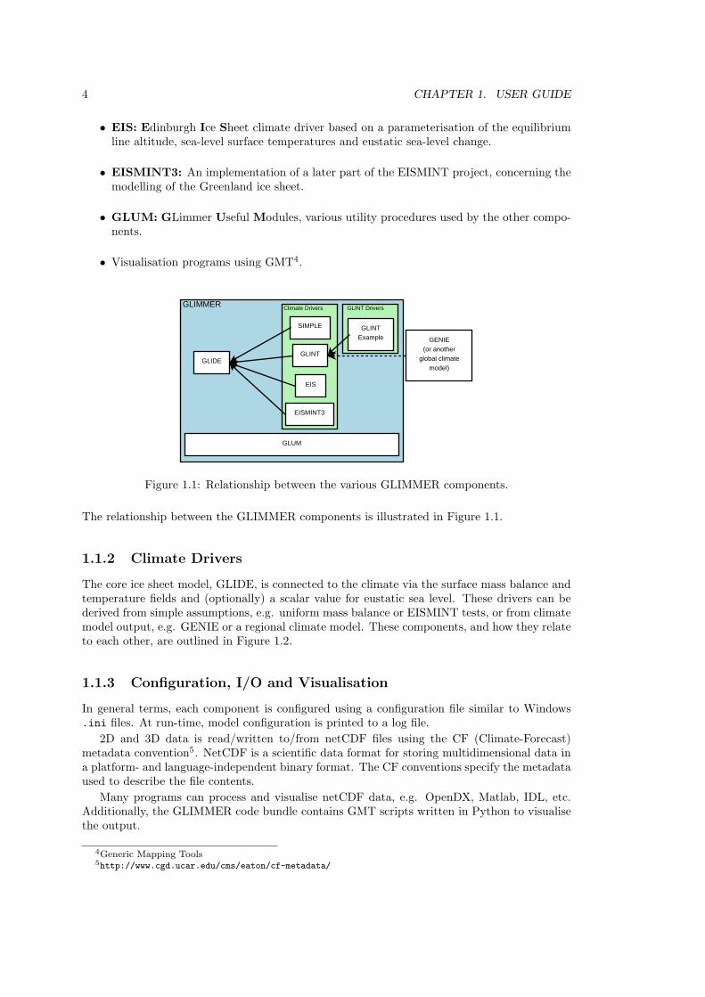
• EIS: Edinburgh Ice Sheet climate driver based on a parameterisation of the equilibriumline altitude, sea-level surface temperatures and eustatic sea-level change.
• EISMINT3: An implementation of a later part of the EISMINT project, concerning themodelling of the Greenland ice sheet.
• GLUM: GLimmer Useful Modules, various utility procedures used by the other compo-nents.
• Visualisation programs using GMT4.
GENIE(or another
global climatemodel)
GLIMMER
GLUM
GLIDEGLINT
EIS
SIMPLE
Climate Drivers
EISMINT3
GLINTExample
GLINT Drivers
Figure 1.1: Relationship between the various GLIMMER components.
The relationship between the GLIMMER components is illustrated in Figure 1.1.
1.1.2 Climate Drivers
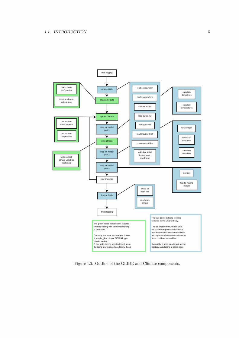
The core ice sheet model, GLIDE, is connected to the climate via the surface mass balance andtemperature fields and (optionally) a scalar value for eustatic sea level. These drivers can bederived from simple assumptions, e.g. uniform mass balance or EISMINT tests, or from climatemodel output, e.g. GENIE or a regional climate model. These components, and how they relateto each other, are outlined in Figure 1.2.
1.1.3 Configuration, I/O and Visualisation
In general terms, each component is configured using a configuration file similar to Windows.ini files. At run-time, model configuration is printed to a log file.
2D and 3D data is read/written to/from netCDF files using the CF (Climate-Forecast)metadata convention5. NetCDF is a scientific data format for storing multidimensional data ina platform- and language-independent binary format. The CF conventions specify the metadataused to describe the file contents.
Many programs can process and visualise netCDF data, e.g. OpenDX, Matlab, IDL, etc.Additionally, the GLIMMER code bundle contains GMT scripts written in Python to visualisethe output.
4Generic Mapping Tools5http://www.cgd.ucar.edu/cms/eaton/cf-metadata/
1.1. INTRODUCTION 5
The blue boxes indicate routinessupplied by the GLIDE library.
The ice sheet communicates withthe surrounding climate via surfacetemperature and mass balance fields.Although there is no reason why other fields could not be modified.
It would be a good idea to split out the isostasy calculations at some stage.
The green boxes indicate user suppliedroutines dealing with the climate forcingof the model.
Currently, there are two example drivers:1. simple_glide: simple EISMINT type climate forcing.2. eis_glide: the ice sheet is forced usingthe same functions as I used in my thesis
finalise Glide
start logging
finish logging
intialise Glide
intialise Climate
read climateconfiguration
initialise climatecalculations
set surfacemass balance
set surfacetemperature
write netCDFclimate variables
(optional)
read configuration
scale parameters
allocate arrays
load sigma file
configure I/O
read input netCDF
create output files
calculate initialtemperature distribution
close allopen files
deallocatearrays
calculatederivatives
calculatetemperatures
calculatevelocities
write output
evolve icethickness
update Climate
step ice modelpart 1
new time step
step ice modelpart 2
write climate
step ice modelpart 3
isostasy
handle marinemargin
Figure 1.2: Outline of the GLIDE and Climate components.
6 CHAPTER 1. USER GUIDE
1.2 Getting and Installing GLIMMER
GLIMMER is a relatively complex system of libraries and programs which build on other li-braries. This section documents how to get GLIMMER and its prerequisites, compile and installit. Please report problems and bugs to the GLIMMER mailing list6.
1.2.1 Prerequisites
GLIMMER is distributed as source code; a sane build environment is therefore required tocompile the model. On UNIX systems GNU make7 is suggested, since the Makefiles may relyon some GNU make specific features. There are two ways of getting the source code:
1. download a released version from the GLIMMER website89, or
2. download the latest developers’ version of GLIMMER and friends from NeSCForge10 usingCVS11.
For beginners, the latest release is recommended. More experienced users may want to try theCVS version, as it will have all the latest bug-fixes and new features.
In either case, a good f95 compiler is required. GLIMMER is known to work with theNAGware f95, Intel ifort and later versions of GNU gfortran compilers. GLIMMER does notcompile with the SUNWS 7.0 f95 compiler due to a compiler bug. The current SUN f95 compilermight work, but has not been tested yet.
The other important prerequisite is the netCDF12 library, which GLIMMER uses for dataI/O. You will most likely need to compile and install the netCDF library yourself, since thebinary packages usually do not contain the Fortran 90 bindings which are used by GLIMMER.
Additional packages are required if you want to build GLIMMER from CVS. You need GNUautoconf and automake to generate the build system, as well as Python13, which is used foranalysing dependencies and for automatically generating parts of the code. Furthermore, thePython scripts rely on language features which were only introduced with Python version 2.3.
1.2.2 The GLIMMER Directory Structure
The following commands describe the setup if you use the bash shell. The setup works sim-ilarly for other shells. We suggest that you install glimmer and friends in its own directory,e.g. /home/user/glimmer. Assign the shell variable $GLIMMER PREFIX to this directory, i.e.export GLIMMER PREFIX=/home/user/glimmer. This directory will contain the following sub–directories:
6http://forge.nesc.ac.uk/mailman/listinfo/glimmer-discuss7http://www.gnu.org/software/make/8http://glimmer.forge.nesc.ac.uk9http://glimmer.forge.nesc.ac.uk
10http://forge.nesc.ac.uk/11http://www.gnu.org/software/cvs/12http://www.unidata.ucar.edu/packages/netcdf/index.html13http://www.python.org
1.2. GETTING AND INSTALLING GLIMMER 7
$GLIMMER PREFIX/bin executables are installed in this directory. Setyour path to include this directory, i.e. export
PATH=$PATH:$GLIMMER PREFIX/bin.$GLIMMER PREFIX/include include and f95 module files will be installed in this directory. If
you want to compile your own climate drivers set the compilersearch path to include this directory.
$GLIMMER PREFIX/lib the libraries get installed here. Set your linker to look in thisdirectory for the GLIMMER libraries if you want to compileyour own climate drivers.
$GLIMMER PREFIX/share data files get installed here.$GLIMMER PREFIX/src this is the only directory you need to create yourself. Unpack
the GLIMMER sources here.
1.2.3 Installing a Released Version of GLIMMER
Download the GLIMMER tarball from the GLIMMER site and unpack it in the $GLIMMER PREFIX/src
directory using
tar -xvzf glimmer-VERS.tar.gz
where VERS is the package version.The package is then compiled using the usual GNU sequence of commands:
./configure --prefix=$GLIMMER_PREFIX [other_options]
make
make install
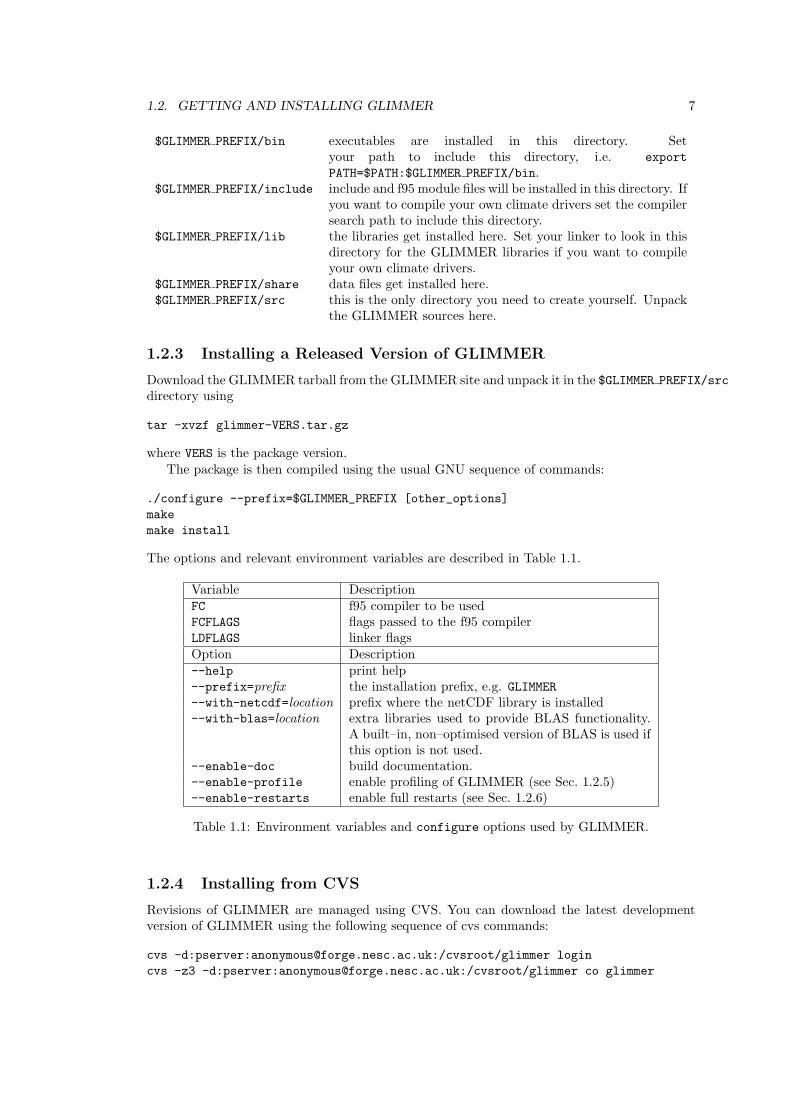
The options and relevant environment variables are described in Table 1.1.
Variable DescriptionFC f95 compiler to be usedFCFLAGS flags passed to the f95 compilerLDFLAGS linker flagsOption Description--help print help--prefix=prefix the installation prefix, e.g. GLIMMER--with-netcdf=location prefix where the netCDF library is installed--with-blas=location extra libraries used to provide BLAS functionality.
A built–in, non–optimised version of BLAS is used ifthis option is not used.
--enable-doc build documentation.--enable-profile enable profiling of GLIMMER (see Sec. 1.2.5)--enable-restarts enable full restarts (see Sec. 1.2.6)
Table 1.1: Environment variables and configure options used by GLIMMER.
1.2.4 Installing from CVS
Revisions of GLIMMER are managed using CVS. You can download the latest developmentversion of GLIMMER using the following sequence of cvs commands:
cvs -d:pserver:[email protected]:/cvsroot/glimmer login
cvs -z3 -d:pserver:[email protected]:/cvsroot/glimmer co glimmer
8 CHAPTER 1. USER GUIDE
The cvs version does not include some automatically generated files. In order to be ableto compile the cvs version you need the GNU autotools and python. The build scripts aregenerated by running
./bootstrap
in the $GLIMMER PREFIX/src directory. The package is then configured and built as describedin Section 1.2.3.
1.2.5 Profiling
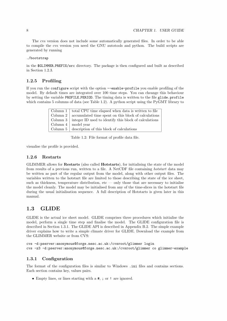
If you run the configure script with the option --enable-profile you enable profiling of themodel. By default times are integrated over 100 time steps. You can cheange this behaviourby setting the variable PROFILE PERIOD. The timing data is written to the file glide.profilewhich contains 5 columns of data (see Table 1.2). A python script using the PyGMT library to
Column 1 total CPU time elapsed when data is written to fileColumn 2 accumulated time spent on this block of calculationsColumn 3 integer ID used to identify this block of calculationsColumn 4 model yearColumn 5 description of this block of calculations
Table 1.2: File format of profile data file.
visualise the profile is provided.
1.2.6 Restarts
GLIMMER allows for Restarts (also called Hotstarts), for initialising the state of the modelfrom results of a previous run, written to a file. A NetCDF file containing hotstart data maybe written as part of the regular output from the model, along with other output files. Thevariables written to the hotstart file are limited to those describing the state of the ice sheet,such as thickness, temperature distribution, etc — only those that are necessary to initialisethe model cleanly. The model may be initialised from any of the time-slices in the hotstart fileduring the usual initialisation sequence. A full description of Hotstarts is given later in thismanual.
1.3 GLIDE
GLIDE is the actual ice sheet model. GLIDE comprises three procedures which initialise themodel, perform a single time step and finalise the model. The GLIDE configuration file isdescribed in Section 1.3.1. The GLIDE API is described in Appendix B.2. The simple exampledriver explains how to write a simple climate driver for GLIDE. Download the example fromthe GLIMMER website or from CVS:
cvs -d:pserver:[email protected]:/cvsroot/glimmer login
cvs -z3 -d:pserver:[email protected]:/cvsroot/glimmer co glimmer-example
1.3.1 Configuration
The format of the configuration files is similar to Windows .ini files and contains sections.Each section contains key, values pairs.
• Empty lines, or lines starting with a #, ; or ! are ignored.
1.3. GLIDE 9
• A new section starts with the the section name enclose with square brackets, e.g. [grid].
• Keys are separated from their associated values by a = or :.
Sections and keys are case sensitive and may contain white space. However, the configurationparser is very simple and thus the number of spaces within a key or section name also matters.Sensible defaults are used when a specific key is not found.
For consistency, options for both the shallow-ice and higher-order dynamical cores (dycore)are discussed. Currently, only the shallow ice dycore is scientifically supported. The higher-orderdycore will be supported as part of planned future releases of Glimmer CISM. Configurationnumber options with a * after them are specific to the higher-order dycore.
[grid]
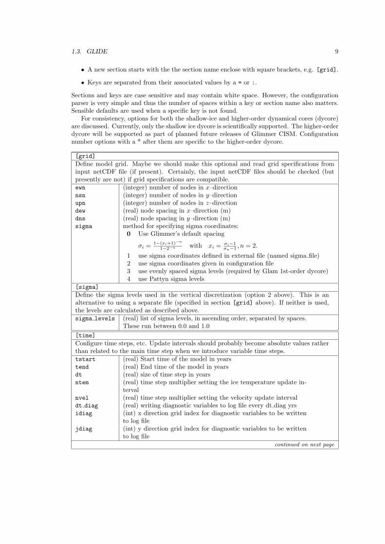
Define model grid. Maybe we should make this optional and read grid specifications frominput netCDF file (if present). Certainly, the input netCDF files should be checked (butpresently are not) if grid specifications are compatible.ewn (integer) number of nodes in x–directionnsn (integer) number of nodes in y–directionupn (integer) number of nodes in z–directiondew (real) node spacing in x–direction (m)dns (real) node spacing in y–direction (m)sigma method for specifying sigma coordinates:
0 Use Glimmer’s default spacing
σi =1−(xi+1)−n
1−2−n with xi =σi−1σn−1 , n = 2.
1 use sigma coordinates defined in external file (named sigma file)2 use sigma coordinates given in configuration file3 use evenly spaced sigma levels (required by Glam 1st-order dycore)4 use Pattyn sigma levels
[sigma]
Define the sigma levels used in the vertical discretization (option 2 above). This is analternative to using a separate file (specified in section [grid] above). If neither is used,the levels are calculated as described above.sigma levels (real) list of sigma levels, in ascending order, separated by spaces.
These run between 0.0 and 1.0
[time]
Configure time steps, etc. Update intervals should probably become absolute values ratherthan related to the main time step when we introduce variable time steps.tstart (real) Start time of the model in yearstend (real) End time of the model in yearsdt (real) size of time step in yearsntem (real) time step multiplier setting the ice temperature update in-
tervalnvel (real) time step multiplier setting the velocity update intervaldt diag (real) writing diagnostic variables to log file every dt diag yrsidiag (int) x direction grid index for diagnostic variables to be written
to log filejdiag (int) y direction grid index for diagnostic variables to be written
to log filecontinued on next page
10 CHAPTER 1. USER GUIDE
continued from previous page
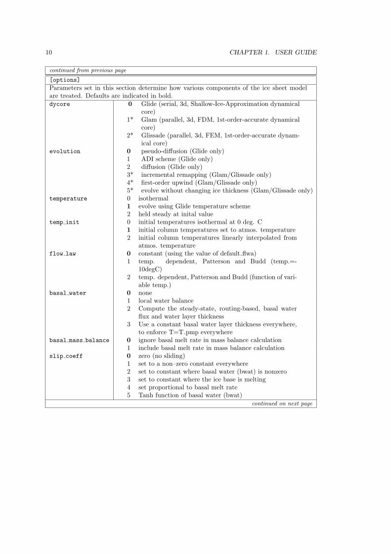
[options]
Parameters set in this section determine how various components of the ice sheet modelare treated. Defaults are indicated in bold.dycore 0 Glide (serial, 3d, Shallow-Ice-Approximation dynamical
core)1* Glam (parallel, 3d, FDM, 1st-order-accurate dynamical
core)2* Glissade (parallel, 3d, FEM, 1st-order-accurate dynam-
ical core)evolution 0 pseudo-diffusion (Glide only)
1 ADI scheme (Glide only)2 diffusion (Glide only)3* incremental remapping (Glam/Glissade only)4* first-order upwind (Glam/Glissade only)5* evolve without changing ice thickness (Glam/Glissade only)
temperature 0 isothermal1 evolve using Glide temperature scheme2 held steady at inital value
temp init 0 initial temperatures isothermal at 0 deg. C1 initial column temperatures set to atmos. temperature2 initial column temperatures linearly interpolated from
atmos. temperatureflow law 0 constant (using the value of default flwa)
1 temp. dependent, Patterson and Budd (temp.=-10degC)
2 temp. dependent, Patterson and Budd (function of vari-able temp.)
basal water 0 none1 local water balance2 Compute the steady-state, routing-based, basal water
flux and water layer thickness3 Use a constant basal water layer thickness everywhere,
to enforce T=T pmp everywherebasal mass balance 0 ignore basal melt rate in mass balance calculation
1 include basal melt rate in mass balance calculationslip coeff 0 zero (no sliding)
1 set to a non–zero constant everywhere2 set to constant where basal water (bwat) is nonzero3 set to constant where the ice base is melting4 set proportional to basal melt rate5 Tanh function of basal water (bwat)
continued on next page
1.3. GLIDE 11
continued from previous page
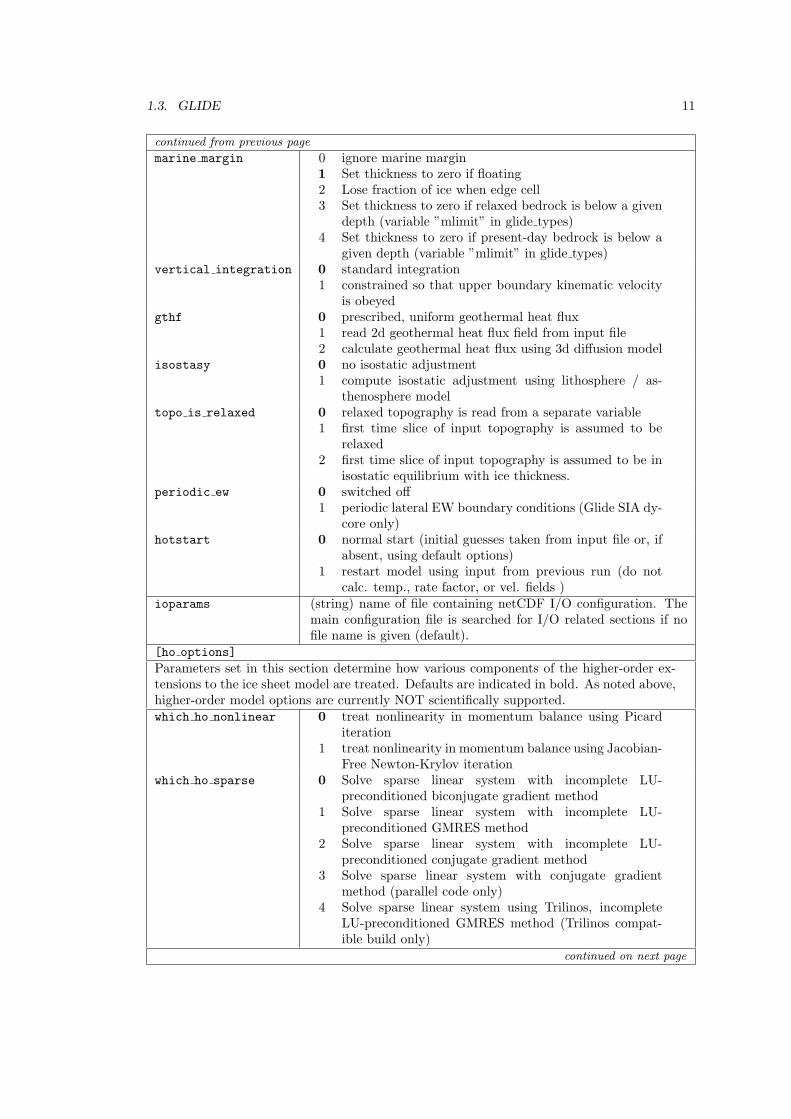
marine margin 0 ignore marine margin1 Set thickness to zero if floating2 Lose fraction of ice when edge cell3 Set thickness to zero if relaxed bedrock is below a given
depth (variable ”mlimit” in glide types)4 Set thickness to zero if present-day bedrock is below a
given depth (variable ”mlimit” in glide types)vertical integration 0 standard integration
1 constrained so that upper boundary kinematic velocityis obeyed
gthf 0 prescribed, uniform geothermal heat flux1 read 2d geothermal heat flux field from input file2 calculate geothermal heat flux using 3d diffusion model
isostasy 0 no isostatic adjustment1 compute isostatic adjustment using lithosphere / as-
thenosphere modeltopo is relaxed 0 relaxed topography is read from a separate variable
1 first time slice of input topography is assumed to berelaxed
2 first time slice of input topography is assumed to be inisostatic equilibrium with ice thickness.
periodic ew 0 switched off1 periodic lateral EW boundary conditions (Glide SIA dy-
core only)hotstart 0 normal start (initial guesses taken from input file or, if
absent, using default options)1 restart model using input from previous run (do not
calc. temp., rate factor, or vel. fields )ioparams (string) name of file containing netCDF I/O configuration. The
main configuration file is searched for I/O related sections if nofile name is given (default).
[ho options]
Parameters set in this section determine how various components of the higher-order ex-tensions to the ice sheet model are treated. Defaults are indicated in bold. As noted above,higher-order model options are currently NOT scientifically supported.which ho nonlinear 0 treat nonlinearity in momentum balance using Picard
iteration1 treat nonlinearity in momentum balance using Jacobian-
Free Newton-Krylov iterationwhich ho sparse 0 Solve sparse linear system with incomplete LU-
preconditioned biconjugate gradient method1 Solve sparse linear system with incomplete LU-
preconditioned GMRES method2 Solve sparse linear system with incomplete LU-
preconditioned conjugate gradient method3 Solve sparse linear system with conjugate gradient
method (parallel code only)4 Solve sparse linear system using Trilinos, incomplete
LU-preconditioned GMRES method (Trilinos compat-ible build only)
continued on next page
12 CHAPTER 1. USER GUIDE
continued from previous page
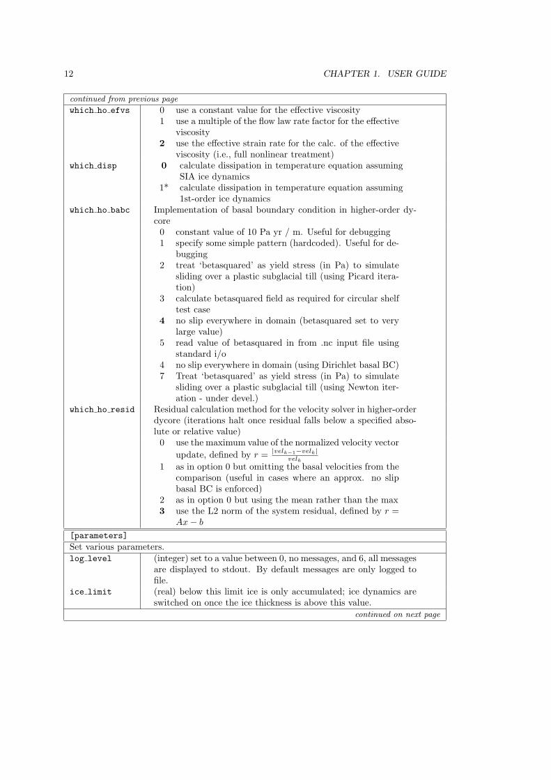
which ho efvs 0 use a constant value for the effective viscosity1 use a multiple of the flow law rate factor for the effective
viscosity2 use the effective strain rate for the calc. of the effective
viscosity (i.e., full nonlinear treatment)which disp 0 calculate dissipation in temperature equation assuming
SIA ice dynamics1* calculate dissipation in temperature equation assuming
1st-order ice dynamicswhich ho babc Implementation of basal boundary condition in higher-order dy-
core0 constant value of 10 Pa yr / m. Useful for debugging1 specify some simple pattern (hardcoded). Useful for de-
bugging2 treat ‘betasquared’ as yield stress (in Pa) to simulate
sliding over a plastic subglacial till (using Picard itera-tion)
3 calculate betasquared field as required for circular shelftest case
4 no slip everywhere in domain (betasquared set to verylarge value)
5 read value of betasquared in from .nc input file usingstandard i/o
4 no slip everywhere in domain (using Dirichlet basal BC)7 Treat ‘betasquared’ as yield stress (in Pa) to simulate
sliding over a plastic subglacial till (using Newton iter-ation - under devel.)
which ho resid Residual calculation method for the velocity solver in higher-orderdycore (iterations halt once residual falls below a specified abso-lute or relative value)0 use the maximum value of the normalized velocity vector
update, defined by r = |velk−1−velk|velk
1 as in option 0 but omitting the basal velocities from thecomparison (useful in cases where an approx. no slipbasal BC is enforced)
2 as in option 0 but using the mean rather than the max3 use the L2 norm of the system residual, defined by r =
Ax− b
[parameters]
Set various parameters.log level (integer) set to a value between 0, no messages, and 6, all messages
are displayed to stdout. By default messages are only logged tofile.
ice limit (real) below this limit ice is only accumulated; ice dynamics areswitched on once the ice thickness is above this value.
continued on next page
1.3. GLIDE 13
continued from previous page
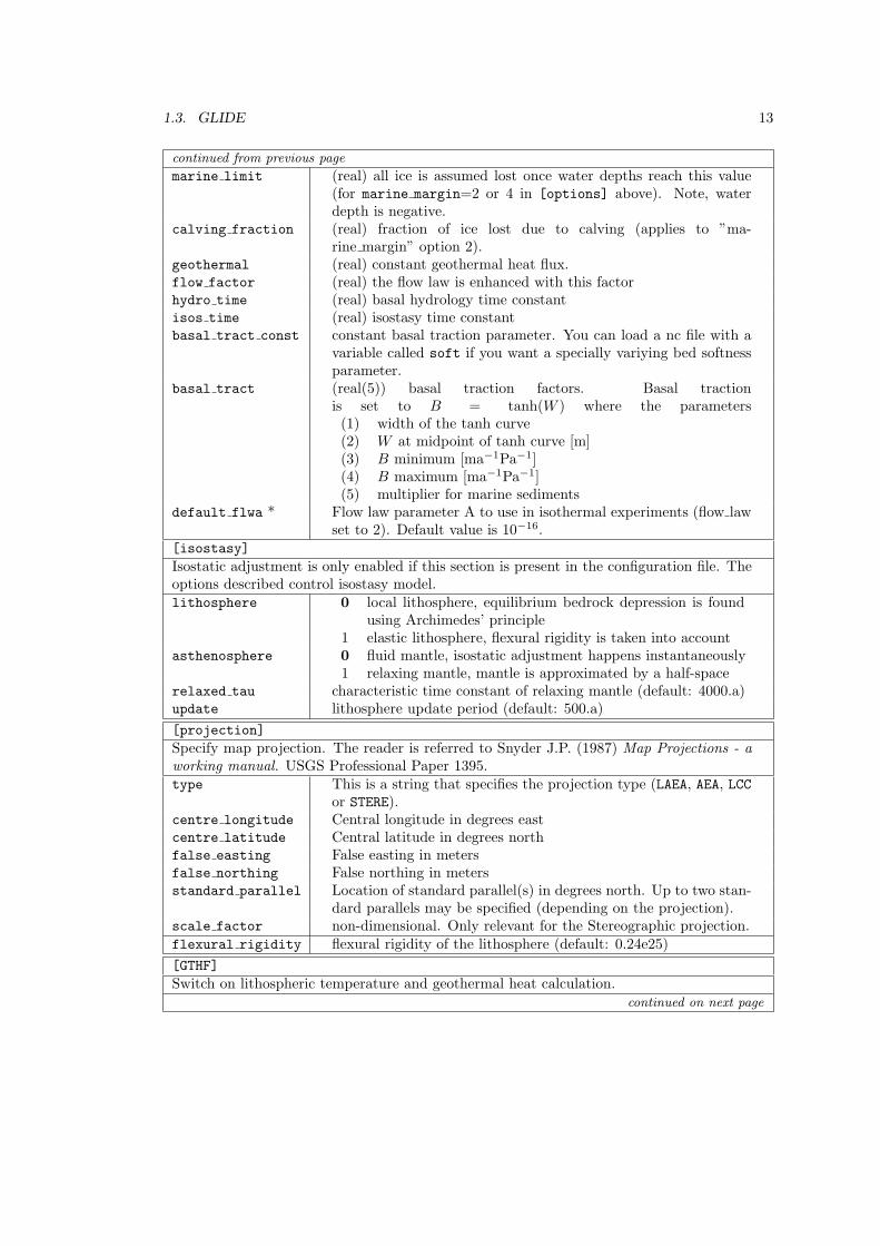
marine limit (real) all ice is assumed lost once water depths reach this value(for marine margin=2 or 4 in [options] above). Note, waterdepth is negative.
calving fraction (real) fraction of ice lost due to calving (applies to ”ma-rine margin” option 2).
geothermal (real) constant geothermal heat flux.flow factor (real) the flow law is enhanced with this factorhydro time (real) basal hydrology time constantisos time (real) isostasy time constantbasal tract const constant basal traction parameter. You can load a nc file with a
variable called soft if you want a specially variying bed softnessparameter.
basal tract (real(5)) basal traction factors. Basal tractionis set to B = tanh(W ) where the parameters(1) width of the tanh curve(2) W at midpoint of tanh curve [m](3) B minimum [ma−1Pa−1](4) B maximum [ma−1Pa−1](5) multiplier for marine sediments
default flwa * Flow law parameter A to use in isothermal experiments (flow lawset to 2). Default value is 10−16.
[isostasy]
Isostatic adjustment is only enabled if this section is present in the configuration file. Theoptions described control isostasy model.lithosphere 0 local lithosphere, equilibrium bedrock depression is found
using Archimedes’ principle1 elastic lithosphere, flexural rigidity is taken into account
asthenosphere 0 fluid mantle, isostatic adjustment happens instantaneously1 relaxing mantle, mantle is approximated by a half-space
relaxed tau characteristic time constant of relaxing mantle (default: 4000.a)update lithosphere update period (default: 500.a)
[projection]
Specify map projection. The reader is referred to Snyder J.P. (1987) Map Projections - aworking manual. USGS Professional Paper 1395.type This is a string that specifies the projection type (LAEA, AEA, LCC
or STERE).centre longitude Central longitude in degrees eastcentre latitude Central latitude in degrees northfalse easting False easting in metersfalse northing False northing in metersstandard parallel Location of standard parallel(s) in degrees north. Up to two stan-
dard parallels may be specified (depending on the projection).scale factor non-dimensional. Only relevant for the Stereographic projection.flexural rigidity flexural rigidity of the lithosphere (default: 0.24e25)
[GTHF]
Switch on lithospheric temperature and geothermal heat calculation.continued on next page
14 CHAPTER 1. USER GUIDE
continued from previous page
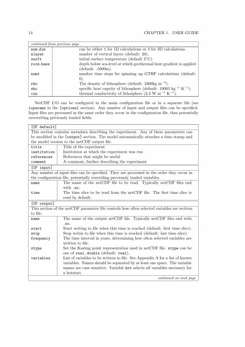
num dim can be either 1 for 1D calculations or 3 for 3D calculations.nlayer number of vertical layers (default: 20).surft initial surface temperature (default 2◦C).rock base depth below sea-level at which geothermal heat gradient is applied
(default: -5000m).numt number time steps for spinning up GTHF calculations (default:
0).rho The density of lithosphere (default: 3300kg m−3).shc specific heat capcity of lithosphere (default: 1000J kg−1 K−1).con thermal conductivity of lithosphere (3.3 W m−1 K−1).
NetCDF I/O can be configured in the main configuration file or in a separate file (seeioparams in the [options] section). Any number of input and output files can be specified.Input files are processed in the same order they occur in the configuration file, thus potentiallyoverwriting priviously loaded fields.
[CF default]
This section contains metadata describing the experiment. Any of these parameters canbe modified in the [output] section. The model automatically attaches a time stamp andthe model version to the netCDF output file.title Title of the experimentinstitution Institution at which the experiment was runreferences References that might be usefulcomment A comment, further describing the experiment
[CF input]
Any number of input files can be specified. They are processed in the order they occur inthe configuration file, potentially overriding previously loaded variables.name The name of the netCDF file to be read. Typically netCDF files end
with .nc.time The time slice to be read from the netCDF file. The first time slice is
read by default.
[CF output]
This section of the netCDF parameter file controls how often selected variables are writtento file.name The name of the output netCDF file. Typically netCDF files end with
.nc.start Start writing to file when this time is reached (default: first time slice).stop Stop writin to file when this time is reached (default: last time slice).frequency The time interval in years, determining how often selected variables are
written to file.xtype Set the floating point representation used in netCDF file. xtype can be
one of real, double (default: real).variables List of variables to be written to file. See Appendix A for a list of known
variables. Names should be separated by at least one space. The variablenames are case sensitive. Variable hot selects all variables necessary fora hotstart.
continued on next page
1.4. EXAMPLE CLIMATE DRIVERS 15
continued from previous page
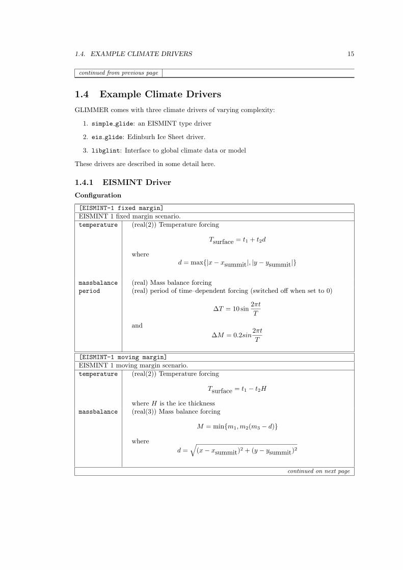
1.4 Example Climate Drivers
GLIMMER comes with three climate drivers of varying complexity:
1. simple glide: an EISMINT type driver
2. eis glide: Edinburh Ice Sheet driver.
3. libglint: Interface to global climate data or model
These drivers are described in some detail here.
1.4.1 EISMINT Driver
Configuration
[EISMINT-1 fixed margin]
EISMINT 1 fixed margin scenario.temperature (real(2)) Temperature forcing
Tsurface = t1 + t2d
whered = max{|x− xsummit|, |y − ysummit|}
massbalance (real) Mass balance forcingperiod (real) period of time–dependent forcing (switched off when set to 0)
∆T = 10 sin2πt
T
and
∆M = 0.2sin2πt
T
[EISMINT-1 moving margin]
EISMINT 1 moving margin scenario.temperature (real(2)) Temperature forcing
Tsurface = t1 − t2H
where H is the ice thicknessmassbalance (real(3)) Mass balance forcing
M = min{m1,m2(m3 − d)}
where
d =√(x− xsummit)
2 + (y − ysummit)2
continued on next page
16 CHAPTER 1. USER GUIDE
continued from previous page
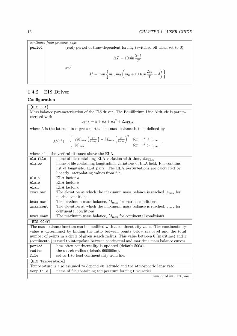
period (real) period of time–dependent forcing (switched off when set to 0)
∆T = 10 sin2πt
T
and
M = min
{m1,m2
(m3 + 100sin
2πt
T− d
)}
1.4.2 EIS Driver
Configuration
[EIS ELA]
Mass balance parameterisation of the EIS driver. The Equilibrium Line Altitude is param-eterised with
zELA = a+ bλ+ cλ2 +∆zELA,
where λ is the latitude in degrees north. The mass balance is then defined by
M(z∗) =
{2Mmax
(z∗
zmax
)−Mmax
(z∗
zmax
)2for z∗ ≤ zmax
Mmax for z∗ > zmax
,
where z∗ is the vertical distance above the ELA.ela file name of file containing ELA variation with time, ∆zELA
ela ew name of file containing longitudinal variations of ELA field. File containslist of longitude, ELA pairs. The ELA perturbations are calculated bylinearly interpolating values from file.
ela a ELA factor aela b ELA factor bela c ELA factor czmax mar The elevation at which the maximum mass balance is reached, zmax for
marine conditionsbmax mar The maximum mass balance, Mmax for marine conditionszmax cont The elevation at which the maximum mass balance is reached, zmax for
continental conditionsbmax cont The maximum mass balance, Mmax for continental conditions
[EIS CONY]
The mass balance function can be modified with a continentality value. The continentalityvalue is determined by finding the ratio between points below sea level and the totalnumber of points in a circle of given search radius. This value between 0 (maritime) and 1(continental) is used to interpolate between continental and maritime mass balance curves.period how often continentality is updated (default 500a).radius the search radius (default 600000m).file set to 1 to load continentality from file.
[EIS Temperature]
Temperature is also assumed to depend on latitude and the atmospheric lapse rate.temp file name of file containing temperature forcing time series.
continued on next page
1.4. EXAMPLE CLIMATE DRIVERS 17
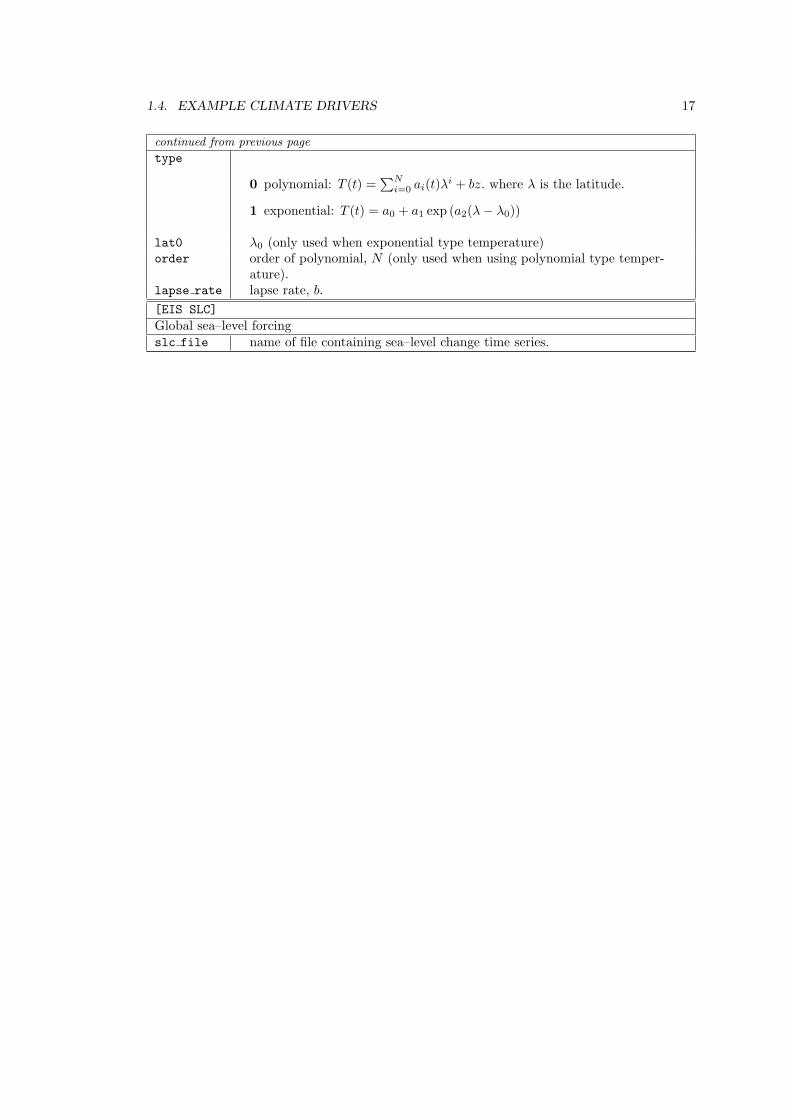
continued from previous page
type
0 polynomial: T (t) =∑N
i=0 ai(t)λi + bz. where λ is the latitude.
1 exponential: T (t) = a0 + a1 exp (a2(λ− λ0))
lat0 λ0 (only used when exponential type temperature)order order of polynomial, N (only used when using polynomial type temper-
ature).lapse rate lapse rate, b.
[EIS SLC]
Global sea–level forcingslc file name of file containing sea–level change time series.
18 CHAPTER 1. USER GUIDE
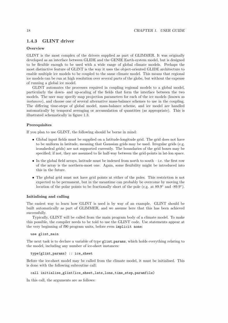
1.4.3 GLINT driver
Overview
GLINT is the most complex of the drivers supplied as part of GLIMMER. It was originallydeveloped as an interface between GLIDE and the GENIE Earth-system model, but is designedto be flexible enough to be used with a wide range of global climate models. Perhaps themost distinctive feature of GLINT is the way it uses the object-oriented GLIDE architecture toenable multiple ice models to be coupled to the same climate model. This means that regionalice models can be run at high resolution over several parts of the globe, but without the expenseof running a global ice model.
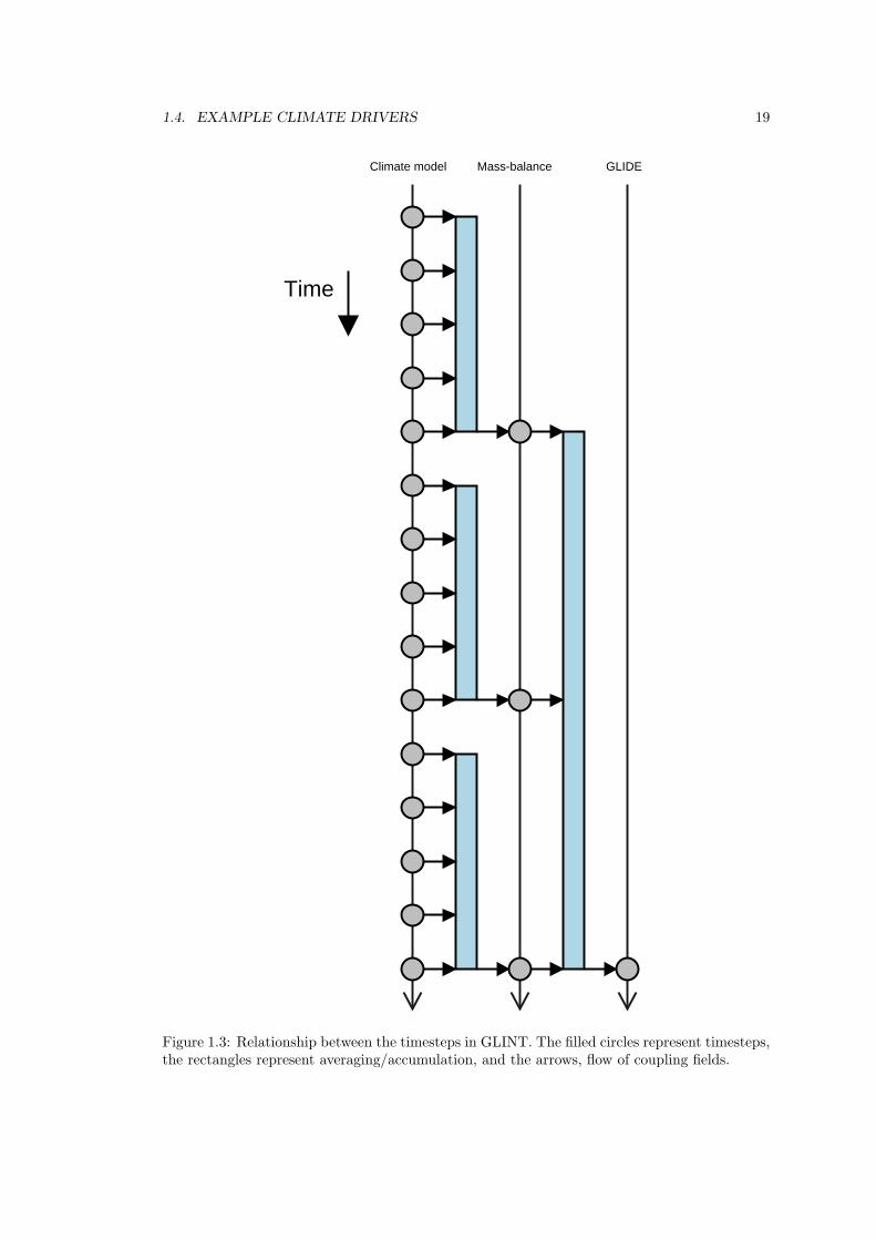
GLINT automates the processes required in coupling regional models to a global model,particularly the down- and up-scaling of the fields that form the interface between the twomodels. The user may specify map projection parameters for each of the ice models (known asinstances), and choose one of several alternative mass-balance schemes to use in the coupling.The differing time-steps of global model, mass-balance scheme, and ice model are handledautomatically by temporal averaging or accumulation of quantities (as appropriate). This isillustrated schematically in figure 1.3.
Prerequisites
If you plan to use GLINT, the following should be borne in mind:
• Global input fields must be supplied on a latitude-longitude grid. The grid does not haveto be uniform in latitude, meaning that Gaussian grids may be used. Irregular grids (e.g.icosahedral grids) are not supported currently. The boundaries of the grid boxes may bespecified; if not, they are assumed to lie half-way between the grid-points in lat-lon space.
• In the global field arrays, latitude must be indexed from north to south – i.e. the first rowof the array is the northern-most one. Again, some flexibility might be introduced intothis in the future.
• The global grid must not have grid points at either of the poles. This restriction is notexpected to be permanent, but in the meantime can probably be overcome by moving thelocation of the polar points to be fractionally short of the pole (e.g. at 89.9◦ and -89.9◦).
Initialising and calling
The easiest way to learn how GLINT is used is by way of an example. GLINT should bebuilt automatically as part of GLIMMER, and we assume here that this has been achievedsuccessfully.
Typically, GLINT will be called from the main program body of a climate model. To makethis possible, the compiler needs to be told to use the GLINT code. Use statements appear atthe very beginning of f90 program units, before even implicit none:
use glint_main
The next task is to declare a variable of type glint params, which holds everything relating tothe model, including any number of ice-sheet instances:
type(glint_params) :: ice_sheet
Before the ice-sheet model may be called from the climate model, it must be initialised. Thisis done with the following subroutine call:
call initialise_glint(ice_sheet,lats,lons,time_step,paramfile)
In this call, the arguments are as follows:
1.4. EXAMPLE CLIMATE DRIVERS 19
Time
Climate model Mass-balance GLIDE
Figure 1.3: Relationship between the timesteps in GLINT. The filled circles represent timesteps,the rectangles represent averaging/accumulation, and the arrows, flow of coupling fields.
20 CHAPTER 1. USER GUIDE
• ice sheet is the variable of type glint params defined above;
• lats and lons are one-dimensional arrays giving the locations of the global grid-pointsin latitude and longitude, respectively;
• time step is the intended interval between calls to GLINT, in hours. This is known asthe forcing timestep.
• paramfile is the name of the GLINT configuration file.
The contents of the configuration file will be dealt with later. Having initialised the model, itmay now be called as part of the main climate model time-step loop:
call glint(ice_sheet,time,temp,precip,orog)
The arguments given in this example are the compulsory ones only; a large number of optionalarguments may be specified – these are detailed in the reference section below. The compulsoryarguments are:
• ice sheet is the variable of type glint params defined above;
• time is the current model time, in hours;
• temp is the daily mean 2m global air temperature field, in ◦C;
• precip is the global daily accumulated precipitation field, in mm (water equivalent, mak-ing no distinction between rain, snow, etc.);
• orog is the global orography field, in m.
Two mass-balance schemes, both based on the positive degree day (PDD) method, are suppliedwith GLIMMER, and are available through GLINT. One of these calculates the mass-balance forthe whole year (the Annual PDD scheme), while the other calculates on a daily basis (the DailyPDD scheme). The annual scheme incorporates a stochastic temperature variation to accountfor diurnal and other variations, which means that if this scheme is to be used, GLINT should becalled such that it sees a seasonal temperature variation which has had those variations removed.In practice, this means calling GLINT on a monthly basis, with monthly mean temperatures.For the daily scheme, no such restriction exists, and the scheme should be called at least every6 hours.
Finishing off
After the desired number of time-steps have been run, GLINT may have some tidying up to do.To accomplish this, the subroutine end glint must be called:
call end_glint(ice_sheet)
API
A detailed description of the GLINT API may be found in the appendices.
Configuration
GLINT uses the same configuration file format as the rest of GLIMMER. In the case whereonly one GLIDE instance is used, all the configuration data for GLINT and GLIDE can residein the same file. Where two or more instances are used, a top-level file specifies the numberof model instances and the name of a configuration file for each one. Possible configurationsections specific to GLINT are as follows:
1.4. EXAMPLE CLIMATE DRIVERS 21
[GLINT]
Section specifying number of instances.n instance (integer) Number of instances (default=1)
[GLINT instance]
Specifies the name of an instance-specific configuration file. Unnecessary if we only have oneinstance whose configuration data is in the main config file.name Name of instance-sepcific config file (required).
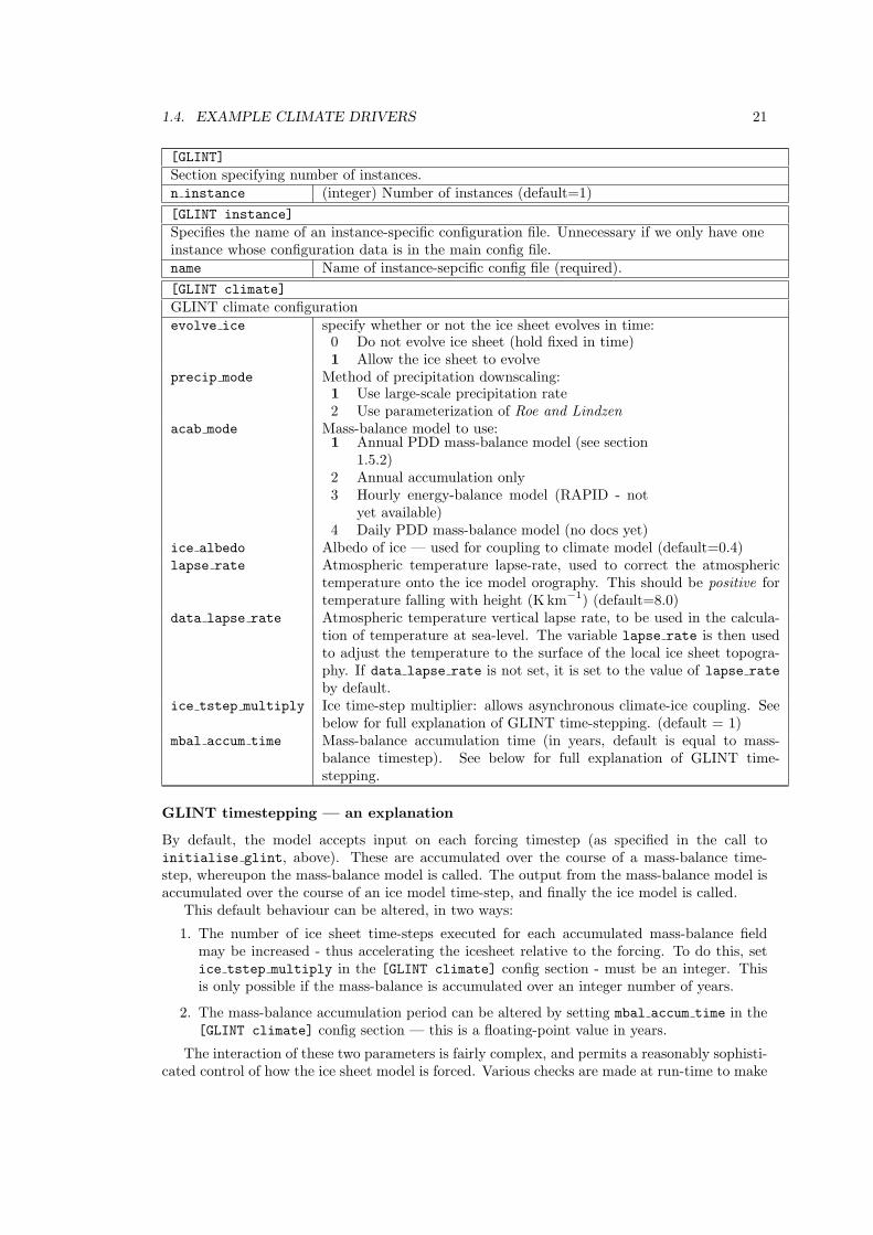
[GLINT climate]
GLINT climate configurationevolve ice specify whether or not the ice sheet evolves in time:
0 Do not evolve ice sheet (hold fixed in time)1 Allow the ice sheet to evolve
precip mode Method of precipitation downscaling:1 Use large-scale precipitation rate2 Use parameterization of Roe and Lindzen
acab mode Mass-balance model to use:1 Annual PDD mass-balance model (see section
1.5.2)2 Annual accumulation only3 Hourly energy-balance model (RAPID - not
yet available)4 Daily PDD mass-balance model (no docs yet)
ice albedo Albedo of ice — used for coupling to climate model (default=0.4)lapse rate Atmospheric temperature lapse-rate, used to correct the atmospheric
temperature onto the ice model orography. This should be positive fortemperature falling with height (Kkm−1) (default=8.0)
data lapse rate Atmospheric temperature vertical lapse rate, to be used in the calcula-tion of temperature at sea-level. The variable lapse rate is then usedto adjust the temperature to the surface of the local ice sheet topogra-phy. If data lapse rate is not set, it is set to the value of lapse rate
by default.ice tstep multiply Ice time-step multiplier: allows asynchronous climate-ice coupling. See
below for full explanation of GLINT time-stepping. (default = 1)mbal accum time Mass-balance accumulation time (in years, default is equal to mass-
balance timestep). See below for full explanation of GLINT time-stepping.
GLINT timestepping — an explanation
By default, the model accepts input on each forcing timestep (as specified in the call toinitialise glint, above). These are accumulated over the course of a mass-balance time-step, whereupon the mass-balance model is called. The output from the mass-balance model isaccumulated over the course of an ice model time-step, and finally the ice model is called.
This default behaviour can be altered, in two ways:
1. The number of ice sheet time-steps executed for each accumulated mass-balance fieldmay be increased - thus accelerating the icesheet relative to the forcing. To do this, setice tstep multiply in the [GLINT climate] config section - must be an integer. Thisis only possible if the mass-balance is accumulated over an integer number of years.
2. The mass-balance accumulation period can be altered by setting mbal accum time in the[GLINT climate] config section — this is a floating-point value in years.
The interaction of these two parameters is fairly complex, and permits a reasonably sophisti-cated control of how the ice sheet model is forced. Various checks are made at run-time to make
22 CHAPTER 1. USER GUIDE
sure sensible/possible values are selected. Most importantly, all relevant time-steps must divideinto one another appropriately - the model will (should. . . ) stop if an un-sensible combinationof values is detected.
GLINT timestepping — further examples
To aid understanding of the time-stepping controls, here are some examples. First, suppose wehave these time-step values:
forcing time-step: 6 hoursmass-balance time-step: 1 dayice time-step: 0.5 year
By default, the model will accumulate 6 months’ worth of mass-balance calculations, andforce the ice sheet model based on that. This might not be desirable, so you could set:
mbal_accum_time = 1.0
This would make GLINT accumulate 1 year’s worth of mass-balance output before forcingthe ice sheet (at which point it would execute two ice sheet time-steps of 0.5 years each).
Having done that, you could accelerate the ice model by a factor of ten, by setting:
ice_tstep_multiply = 10
In this scenario, 20 ice sheet time-steps of 0.5 years each would be done after each 12-monthaccumulation of mass-balance data.
For the second example, we consider the contrasting situation where we don’t want tocalculate a mass-balance on all the available data (perhaps to save time). Consider these time-step values:
forcing time-step: 6 hoursmass-balance time-step: 1 dayice time-step: 10 years
(Clearly this a fairly numerically stable and/or low-resolution ice sheet).To avoid running the daily PDD scheme c.3600 times (depending on the value of days in year),
we can set to only use the first two years of data:
mbal_accum_time = 2.0
GLINT accumulates mass-balance for 2 years, then waits for 8 years (incoming data areignored during this time), before calling the ice sheet. Ice sheet acceleration may be enabledwith ice tstep multiply as before.
1.5 Supplied mass-balance schemes
1.5.1 Overview
The user is, of course, free to supply their own mass-balance model for use with GLIDE. However,GLIMMER includes within it a annual positive-degree-day model for mass balance, shortly tobe augmented by a similar daily model and an hourly energy balance model. This section givesdetails of how to configure and call these models.
1.5. SUPPLIED MASS-BALANCE SCHEMES 23
1.5.2 Annual PDD scheme
The annual PDD scheme is contained in the f90 module glimmer pdd, and the model parametersare contained in the derived type glimmer pdd params. Configuration data is contained in astandard GLIMMER config file, which needs to be read from file before initialising the mass-balance model. The model is initialised by calling the subroutine glimmer pdd init, and themass-balance may be calculated annually by calling glimmer pdd mbal.
Example of use:
use glimmer_pdd
use glimmer_config
...
type(glimmer_pdd_params) :: pdd_scheme
type(ConfigSection),pointer :: config
...
call glimmer_pdd_init(pdd_scheme,config)
...
call glimmer_pdd_mbal(pdd_scheme,artm,arng,prcp,ablt,acab)
In the subroutine call to glimmer pdd mbal, apart from the parameter variable pdd scheme,there are three input fields (artm, arng and prcp), which are, respectively, the annual meanair temperature, annual temperature half-range, and annual accumulated precipitation fields.The final two arguments are output fields — annual ablation (ablt) and annual mass-balance(acab). All arrays are of type real(sp). Temperatures are degrees Celcius, and precipitation,ablation and mass-balance are measured in m of water equivalent.
Day-degree calculation
The greater part of the information held in the glimmer pdd params derived type comprises alook-up table (the PDD table). The model is implemented this way for computational efficiency.
The table has two dimensions: mean annual air temperature (Ta) (as the second index) andannual air temperature half range (i.e., from July’s mean to the annual mean ∆Ta) (as the firstindex). Following Huybrechts and others [1991], daily air temperatures (T ′
a) are assumed tofollow a sinusoidal cycle
T ′a = Ta +∆Ta cos
(2πt
A
)+R(0, σ) (1.1)
where A is the period of a year and R is a random fluctuation drawn from a normal distributionwith mean 0 ◦C and standard deviation σ ◦C. Huybrechts and others [1991] indicate that thenumber of positive degree days (D, ◦C days) for this temperature series can be evaluated as
D =1
σ√2π
A∫0
T ′a+2.5σ∫0
Ta × exp
(−(Ta − T ′
a)2
2σ2
)dTdt (1.2)
where t is time. The table is completed by evaluating this integral using a public-domainalgorithm (Romberg integration), by Bauer [1961]. The inner and outer integrals are coded
24 CHAPTER 1. USER GUIDE
as two subroutines (inner integral and pdd integrand), which call the Romburg integrationrecursively.
The main parameter needed is the assumed standard deviation of daily air temperatures,which can be set in the configuration file (the default is 5 ◦C).
The positive-degree days are then looked up in the table (as a function of Ta and ∆Ta). Wetake care to check that this look up is in done within the bounds of the table. The final valueof P is determined using bi-linear interpolation given the four nearest entries in the table to theactual values of Ta and ∆Ta.
The remainder of the loop completes the calculation of the ablation and accumulation giventhis value for P .
Mass balance calculation
We use the following symbols: a is total annual ablation; as is potential snow ablation; b0 is thecapacity of the snowpack to hold meltwater by refreezing; the total number of positive degreedays (D); day-degree factors for snow and ice (fs and fi); and the fraction of snowfall that canbe held in the snowpack as refrozen meltwater (Wmax). Note that the day-degree factors havebeen converted from ice to water equivalents using the ratio of densities.
First, determine the depth of superimposed ice (b0) that would have to be formed beforerunoff (mass loss) occurs as a constant fraction (Wmax) of precipitation (P )
b0 = WmaxP. (1.3)
Now determine the amount of snow melt by applying a constant day-degree factor for snow tothe number of positive day-degrees
as = fsD. (1.4)
We now compare the potential amount of snow ablation with the ability of the snow layer toabsorb the melt. Three cases are possible. First, all snow melt is held within the snowpack andno runoff occurs (a = 0). Second, the ability of the snowpack to hold meltwater is exceeded butthe potential snow ablation is still less than the total amount of precipitation so that a = as−b0.Finally, the potential snow melt is greater than the precipitation (amount of snow available), sothat ice melt (ai) has to be considered as well. The total ablation is therefore the sum of snowmelt (total precipitation minus meltwater held in refreezing) and ice melt (deduct from totalnumber of degree days, the number of degree days needed to melt all snowfall and convert toice melt)
a = as + ai = P − b0 + fi
(D − P
fs
). (1.5)
We now have a total annual ablation, and can find total net mass balance as the differencebetween the total annual precipitation and the total annual ablation.
Note that this methodology is fairly standard and stems from a series of Greenland papersby Huybrechts, Letreguilly and Reeh in the early 1990s.
Configuration
The annual PDD scheme is configured using a single section in the configuration file:
[GLIMMER annual pdd]
Specifies parameters for the PDD table and mass-balance calculationdx Table spacing in the x-direction (◦C) (default=1.0)dy Table spacing in the y-direction (◦C) (default=1.0)ix Lower bound of x-axis (◦C) (default=0.0)
continued on next page
1.5. SUPPLIED MASS-BALANCE SCHEMES 25
continued from previous page
iy Lower bound of y-axis (◦C) (default=-50.0)nx Number of values in x-direction (default=31)ny Number of values in x-direction (default=71)wmax Fraction of melted snow that refreezes (default=0.6)pddfac ice PDD factor for ice (m day−1 ◦C−1) (default=0.008)pddfac snow PDD factor for snow (m day−1 ◦C−1) (default=0.003)
References
Bauer (1961) Comm. ACM 4, 255.Huybrechts, Letreguilly and Reeh (1991) Palaeogeography, Palaeoclimatology, Palaeoecology(Global and Planetary Change) 89, 399-412.Letreguilly, Reeh and Huybrechts (1991) Palaeogeography, Palaeoclimatology, Palaeoecology(Global and Planetary Change) 90, 385-394.Letreguilly, Huybrechts and Reeh (1991) Journal of Glaciology 37, 149-157.
1.5.3 Daily PDD scheme
The other PDD scheme supplied with GLIMMER is a daily scheme. This is simpler than theannual scheme in that it does not incorporate any stochastic variations. The mass-balance iscalculated on a daily basis, given the daily mean temperature and half-range, and assuminga sinusoidal diurnal cycle. Consequently, the firn model is more sophisticated than with theannual scheme, and includes a snow-densification parameterization.
Configuration
The daily PDD scheme is configured using a single section in the configuration file:
[GLIMMER daily pdd]
Specifies parameters for the PDD table and mass-balance calculationwmax Fraction of melted snow that refreezes (default=0.6)pddfac ice PDD factor for ice (m day−1 ◦C−1) (default=0.008)pddfac snow PDD factor for snow (m day−1 ◦C−1) (default=0.003)rain threshold Temperature above which precipitation is held to be rain (◦C) (de-
fault=1.0)whichrain Which method to use to partition precipitation into rain and snow:
1 Use sinusoidal diurnal temperature variation2 Use mean temperature only
tau0 Snow densification timescale (s) (default=10 years)constC Snow density profile factor C (m−1) (default=0.0165)firnbound Ice-firn boundary as fraction of density of ice (default=0.872)snowdensity Density of fresh snow (kgm−3) (default=300.0)

26 CHAPTER 1. USER GUIDE
Chapter 2
Tutorial
2.1 Introduction
This tutorial section aims to provide a set of more practical, step-by-step instructions on howto first get GLIMMER started after the successful installation and familiarise yourself with thedifferent climate driver options. In general, this tutorial is intended to address the question:
’I have successfully compiled GLIMMER, now what? Do I have to write my own config files,climate drivers etc? I want to see some ice sheet modelling pronto!’
The really short version of an answer to this is type
glide_launch.py myconfig.config
where myconfig.config is a configuration file for GLIMMER as described in the documenta-tion. If you have a config file and all the necessary data ready, this is how you get GLIMMERstarted.
Assuming that if you are reading this, you probably won’t yet have your own config fileready, so you might want to read on:
2.2 EISMINT: using glimmer-example
As you hopefully already know, the heart of GLIMMER is the actual ice sheet model GLIDE.This is where ice physics are resolved etc. To model an ice sheet using GLIDE, you at leastneed to provide it with information about the mass balance. To get you started with a realsimple example climate driver, download glimmer-example from the project homepage or viaCVS, cd into the directory and type
glide_launch.py example.config
this will kick off a simple EISMINT-1 moving margin type model run. The results are writtento example.nc, use a viewer like ncview to visualise them. Take a look at the example.configfile printed below and read the documentation on the EISMINT type climate driver (section1.4.1) to better understand what is happening:
# configuration for the EISMINT-1 test-case # moving margin
[EISMINT-1 moving margin]
[grid]
# grid sizes
ewn = 31
27
28 CHAPTER 2. TUTORIAL
nsn = 31
upn = 11
dew = 50000
dns = 50000
[options]
temperature = 1
flow_law = 2
isostasy = 0
sliding_law = 4
marine_margin = 2
stress_calc = 2
evolution = 2
basal_water = 2
vertical_integration = 0
[time]
tend = 200000.
dt = 10.
ntem = 1.
nvel = 1.
niso = 1.
[parameters]
flow_factor = 1
geothermal = -42e-3
[CF default]
title: EISMINT-1 moving margin
[CF output]
name: example.nc
frequency: 1000
variables: thk uflx vflx bmlt temp
uvel vvel wvel
The line [EISMINT-1 moving margin] sets the model type for this run to be EISMINT(simple glide binary). This can also be achieved by specifying the correct binary using the -m
flag, e.g.
glide_launch.py -m simple_glide example.config
It is probably advisable to use the -m option instead of specifying the binary using a keyterm,as this will only work for EIS and EISMINT model types. For ease of use, the option wasintegrated in the config file for this example.
The [grid] section sets up the topography for the model run.As this is an EISMINT testcase, there is no ’real’ input topography, but ice is building up
on a flat surface, which is why nothing more but the grid dimensions need to be specified. Beaware that this only works for EISMINT type model runs using simple glide. In this case, themass balance is parameterised as a function of distance from the grid center, resulting in a pointsymmetric ice sheet. The grid used here has a size of 31x31 cells (ewn x nsn), comprises of 11vertical layers (upn = 11) and an internal cell spacing of 5000 (dew and dns).
The [options] sections determines the basic behaviour of the model:
2.3. EIS: USING GLIMMER-TESTS 29
temperature = 1 resolves the temperature over the whole of the 11 layers of ice (insteadof assuming ice to be isothermal), isostasy = 0 turns off the isostasy component, etc. (checkthe documentation).
In the [time] section, the end time of the model run is set to 200000 with a timestep sizeof 10 and keeping all internal update processes (temperature and velocity) in line with thetimesteps by setting their multiplier to 1.
Flow factor and geothermal heat flux parameters are set in the [parameters] section.Finally, in the [CF output] section, the name of the file to store the results is given, together
with the variables that should be dumped to the file and the frequency with which they arewritten to it (every 1000 years). In this example, ice thickness (thk), basal melt temperaturebmlt, ice temperature temp etc is output to the result file every 1000 years. Note that thisoutput frequency is independent of the modelling timesteps.
You might want to try and change some of the parameters, e.g. speed up ice flow byincreasing the flow factor, and re-run the model to see what happens. This is fairly simple andstraight forward example of how to get GLIMMER to do some basic modelling. If you want tosee a bit more of what GLIMMER can do, try the next section.
2.3 EIS: using glimmer-tests
glimmer-tests provides more example configurations, that include both the EISMINT and EISclimate drivers. If you have not already done so, download glimmer-tests via the nescforgepage or CVS, and do the usual
./configure -with-glimmer-prefix=/path/to/GLIMMER/installation
(e.g. /usr/local/GLIMMER)
(if you updated GLIMMER via CVS, you need to do ./bootstrap first.)glimmer-tests is not (yet) a test suite, but will exemplarily show what GLIMMER can do
(see the glimmer-tests README file for detailed information on the tests).Basically glimmer-tests runs GLIMMER using the EISMINT 1 and 2 (and 3) climate
driver (fixed and moving margin type ice sheets with no external mass balance forcing), as wellas the Edinburgh Ice Sheet (EIS) climate driver, using mass balance parameterisation via ELAand temperature forcing. There are a couple of other tests running besides this, e.g. somebenchmarks. If you want to run all the examples, simply do a make in the glimmer-tests
directory, but be aware that running all tests will take a good 12+ hours on a single CPU 3GHZ machine. If you’re too impatient for this, simply do a make in one of the subdirectories,e.g. EISMINT1 and GLIDE will be launched using the EISMINT climate driver, which shoulddeliver you a number of netcdf files with the model results, eg. e1.fm.1.nc containing theEISMINT1 fixed margin results 1, etc. Again, to visualise the results use a viewer like ncview.
If you want a more sophisticated results, try make in the eis directory, which will repeatthe results of ? reconstructing the Fennoscandian ice sheet during the last glacial maximum,using the EIS driver.
2.3.1 A short introduction to the EIS driver parameterisation
Again, check the config file fenscan.config to see the basic parameters for this model run.Have a look at the mb2.data (mass balance forcing via ELA), temp-exp.model (exponentialtype temperature forcing) and specmap.data (sealevel change) data files and compare them tothe EIS driver documentation (section 1.4.2) to get an idea of how things are done.
The first column in every data file is the model time at which the new parameter values areapplied. For the temperature model, the records in the temp-exp.model file
...
30 CHAPTER 2. TUTORIAL
-97000.000000 -17.858964 23.158964 -0.051329
-96000.000000 -20.074036 24.674036 -0.051329
...
correspond to the timesteps -97000 and -96000 (first column - model usually ends at time0) where the parameters a0 (2nd column), a1 (3rd column) and a2 (last column) of the expo-nential temperature model T (t) = a0 + a1 exp (a2(λ− λ0)) (page 16) are updated to reflect anapproximate change in temperature of -2 degrees Celsius.
For EIS, the mass balance is parameterised via the ELA, according to
zELA = a+ bλ+ cλ2 +∆zELA,
given the parameters in the according config file section:
...
[EIS ELA]
ela_file = mb2.data
bmax_mar = 4.
ela_a = 14430.069930
ela_b =-371.765734
ela_c = 2.534965
...
Factors a, b and c are specified together with the maximum mass balance of 4. The latitude λin degrees North is read from the input topography grid. In order to do the ELA forcing overtime, the parameter ∆zELA is varied over time using the ela file mb2.data:
...
-109000 225
-105000 350
...
Similar to the temperature forcing, ∆zELA (column 2) is changed at timestep -10900 (column1), to reflect an ELA 225m above the altitude value calculated using the factors a, b, c and thelatitude λ. At timestep -10500, ELA is rising to 350m above the calculated value.
Where a globally changing ∆zELA is insufficient to reflect disparities in ELA, there are twooptions to fine tune ELA behaviour. First, continentality can be used to introduce a dependencyof mass balance with distance to oceans. The according settings are supplied using the [EIS
CONY] section of the config file (see section 1.4.2). In short, an index is calculated for every gridcell reflecting the ratio of below sealevel cells to land cells within a certain range (defaults to600km). Maximum mass balance values are then scaled between the values given in the [EIS
ELA] section for bmax mar (marine conditions, all cells within range are below sea level) andbmax cont (continenal conditions, all cells within range are above sea level). Alternatively,continentality values between 0 and 1 can be input using a file. Set the according flag file to1 and specify the file containing the cony data using a [CF input] section in the configurationfile (see example for ELA file below). .
In case a more detailed spatial distribution of ELA altitudes is needed, e.g. to reflect specialorographic effects, a map of ∆zELA can be input to the model using a netcdf file, containing avariable ’ela’ on a grid the same size and coordinates as the input topography grid the modelis running on. This ela file is coupled using a [CF input] section in the configuration file
[CF input]
name: ela_1k.nc
resulting in a spatial distribution of ∆zELA being applied to the model. The variation of ELAover time using a global ∆zELA is still applied on top of this ELA forcing file.
2.4. GLINT: USING GLINT-EXAMPLE 31
Note: (Maybe an example containing an ELA forcing file should be added to GLIMMERtest/examples?)
Sealevel changes are forced upon the model in an according way using the specmap.data
file.
2.4 GLINT: using glint-example
If finally you want to see what GLIMMER can do using the GLINT climate driver, downloadthe glint-example and try one of the provided example setups. CD into the directory and tryany of the config examples. Start glint example by typing
glint_example
You will then be asked for a climate configuration file and an ice model configuration file. Forthe climate file, a global example including precipitation and temperature timeseries is provided.To let glint know about it, type
glint_example.config
For the ice model config, there are two examples, Greenland and North America. To choseeither one, type
gland20.config
or
namerica20.config
respectively at the prompt asking for the config file, to start the model. Both models are out-putting three files each, containing different variables. Every 100 years, a file namerica20.hot.ncor gland20.hot.nc, respectively is output, which can be used to hotstart the model later fromany of the recorded stages.
As mentioned above, the model type (binary) to use can be stated in the configuration file,or given using the -m option. Currently, the three model binaries that come with GLIMMER aresimple glide, eis glide and glint example. The simple glide and eis glide drivers that arestarted using the glide launch.py Python script, which needs to know which binary to address.The model binary can also be set as an environment variable $GLIDE MODEL. However, asglint is called directly using the compiled binary glint example here, it is not necessary tofurther specify the model.

32 CHAPTER 2. TUTORIAL
Part II
Developer Documentation
33

Chapter 3
Numerics
This part describes the numerical implementation of GLIMMER in some detail. It is hopedthat more parts will be added in the future.
3.1 Ice Thickness Evolution
The evolution of the ice thickness, H, stems from the continuity equation and can be expressedas
∂H
∂t= −∇ · (uH) +B, (3.1)
where u is the vertically averaged ice velocity, B is the surface mass balance and ∇ is thehorizontal gradient operator (?).
For large–scale ice sheet models, the shallow ice approximation is generally used. Thisapproximation states that bedrock and ice surface slopes are assumed sufficiently small so thatthe normal stress components can be neglected (?). The horizontal shear stresses (τxz and τyz)can thus be approximated by
τxz(z) = −ρg(s− z)∂s
∂x,
τyz(z) = −ρg(s− z)∂s
∂y,
(3.2)
where ρ is the density of ice, g the acceleration due to gravity and s = H + h the ice surface.Strain rates εij of polycrystalline ice are related to the stress tensor by the non–linear flow
law:
εiz =1
2
(∂ui
∂z+
∂uz
∂i
)= A(T ∗)τ
(n−1)∗ τiz i = x, y, (3.3)
where τ∗ is the effective shear stress defined by the second invariant of the stress tensor, n theflow law exponent and A the temperature–dependent flow law coefficient. T ∗ is the absolutetemperature corrected for the dependence of the melting point on pressure (T ∗ = T + 8.7 ·10−4(H + h− z), T in Kelvin, ?). The parameters A and n have to be found by experiment. nis usually taken to be 3. A depends on factors such as temperature, crystal size and orientation,and ice impurities. Experiments suggest that A follows the Arrhenius relationship:
A(T ∗) = fae−Q/RT∗, (3.4)
where a is a temperature–independent material constant, Q is the activation energy for creepand R is the universal gas constant (?). f is a tuning parameter used to ‘speed–up’ ice flowand accounts for ice impurities and the development of anisotropic ice fabrics (????).
35
36 CHAPTER 3. NUMERICS
Integrating (3.4) with respect to z gives the horizontal velocity profile:
u(z)− u(h) = −2(ρg)n|∇s|n−1∇s
z∫h
A(s− z)ndz, (3.5)
where u(h) is the basal velocity (sliding velocity). Integrating (3.5) again with respect to zgives an expression for the vertically averaged ice velocity:
uH = −2(ρg)n|∇s|n−1∇s
s∫h
z∫h
A(s− z)ndzdz′. (3.6)
The vertical ice velocity stems from the conservation of mass for an incompressible material:
∂ux
∂x+
∂uy
∂y+
∂uz
∂z= 0. (3.7)
Integrating (3.7) with respect to z gives the vertical velocity distribution of each ice column:
w(z) = −z∫
h
∇ · u(z)dz + w(h), (3.8)
with lower, kinematic boundary condition
w(h) =∂h
∂t+ u(h) ·∇h+ S, (3.9)
where S is the melt rate at the ice base given by Equation (3.55). The upper kinematic boundaryis given by the surface mass balance and must satisfy:
w(s) =∂s
∂t+ u(s) ·∇s+B. (3.10)
3.1.1 Numerical Grid
The continuous equations descrining ice physics have to be discretised in order to be solved by acomputer (which is inherently finite). This section describes the finite–difference grids employedby the model.
Horizontal Grid
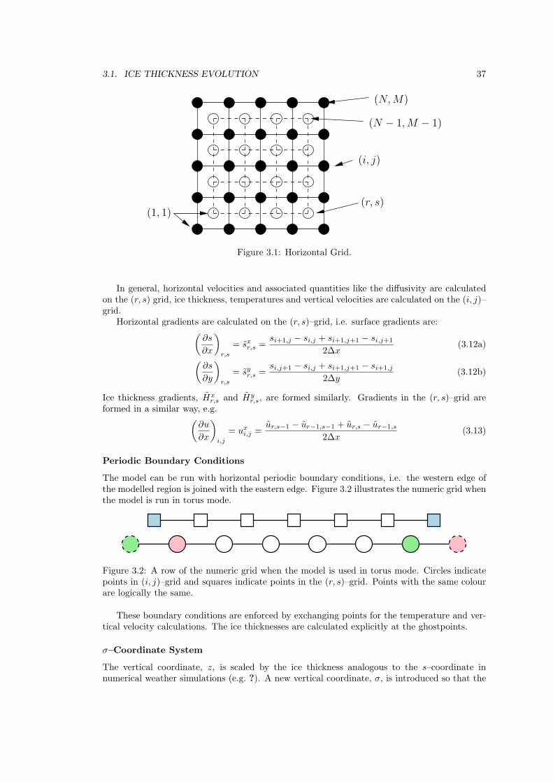
The modelled region (x ∈ [0, Lx], y ∈ [0, Ly]) is discretised using a regular grid so that xi =(i − 1)∆x for i ∈ [1, N ] (and similarly for yj). The model uses two staggered horizontal gridsin order to improve stability. Both grids use the same grid spacing, ∆x and ∆y, but are off-setby half a grid (see Fig. 3.1). Quantities calculated on the (r, s)–grid are denoted with a tilde,i.e. F . Quantities are transformed between grids by averaging over the surrounding nodes, i.e.a quantity in the (i, j)–grid becomes in the (r, s) grid:
Fr,s = Fi+ 12 ,j+
12=
1
4(Fi,j + Fi+1,j + Fi+1,j+1 + Fi,j+1) (3.11a)
and similarly for the reverse transformation:
Fi,j = Fr− 12 ,s−
12=
1
4(Fr−1,s−1 + Fr,s−1 + Fr,s + Fr−1,s) (3.11b)
3.1. ICE THICKNESS EVOLUTION 37
(N − 1,M − 1)
(r, s)
(i, j)
(N,M)
(1, 1)
Figure 3.1: Horizontal Grid.
In general, horizontal velocities and associated quantities like the diffusivity are calculatedon the (r, s) grid, ice thickness, temperatures and vertical velocities are calculated on the (i, j)–grid.
Horizontal gradients are calculated on the (r, s)–grid, i.e. surface gradients are:(∂s
∂x
)r,s
= sxr,s =si+1,j − si,j + si+1,j+1 − si,j+1
2∆x(3.12a)(
∂s
∂y
)r,s
= syr,s =si,j+1 − si,j + si+1,j+1 − si+1,j
2∆y(3.12b)
Ice thickness gradients, Hxr,s and Hy
r,s, are formed similarly. Gradients in the (r, s)–grid areformed in a similar way, e.g.(
∂u
∂x
)i,j
= uxi,j =
ur,s−1 − ur−1,s−1 + ur,s − ur−1,s
2∆x(3.13)
Periodic Boundary Conditions
The model can be run with horizontal periodic boundary conditions, i.e. the western edge ofthe modelled region is joined with the eastern edge. Figure 3.2 illustrates the numeric grid whenthe model is run in torus mode.
Figure 3.2: A row of the numeric grid when the model is used in torus mode. Circles indicatepoints in (i, j)–grid and squares indicate points in the (r, s)–grid. Points with the same colourare logically the same.
These boundary conditions are enforced by exchanging points for the temperature and ver-tical velocity calculations. The ice thicknesses are calculated explicitly at the ghostpoints.
σ–Coordinate System
The vertical coordinate, z, is scaled by the ice thickness analogous to the s–coordinate innumerical weather simulations (e.g. ?). A new vertical coordinate, σ, is introduced so that the
38 CHAPTER 3. NUMERICS
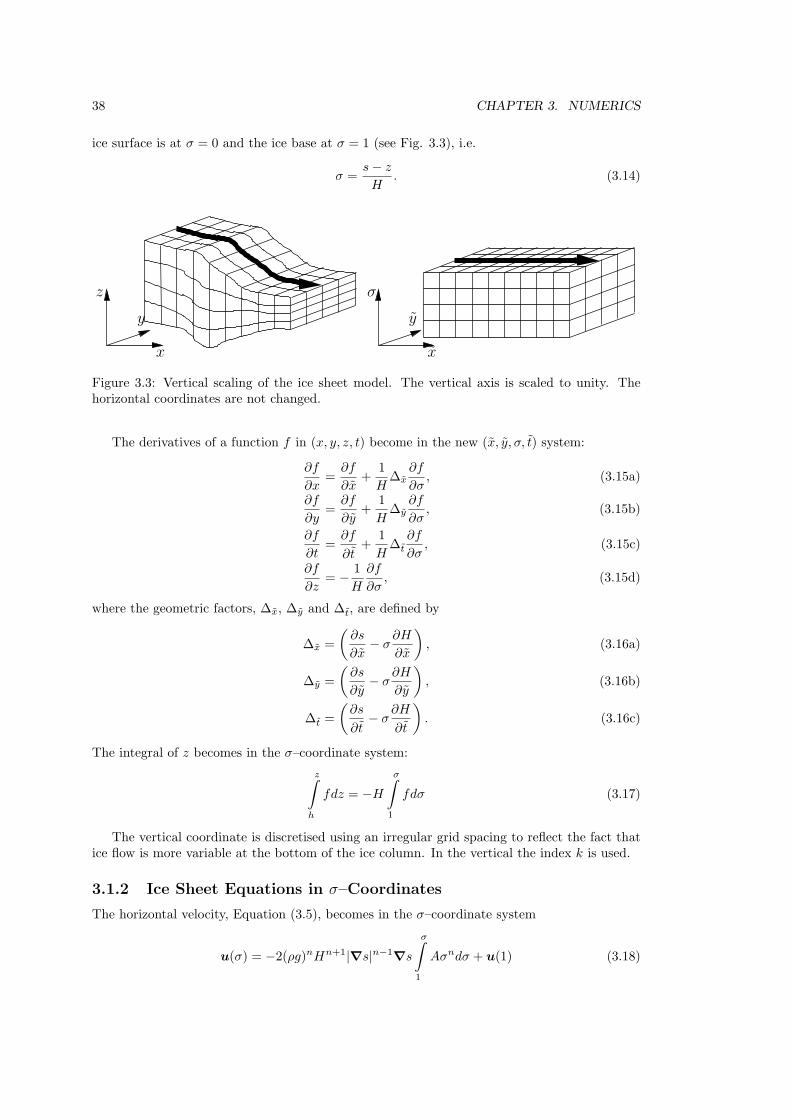
ice surface is at σ = 0 and the ice base at σ = 1 (see Fig. 3.3), i.e.
σ =s− z
H. (3.14)
x
z
y
x
σ
y
Figure 3.3: Vertical scaling of the ice sheet model. The vertical axis is scaled to unity. Thehorizontal coordinates are not changed.
The derivatives of a function f in (x, y, z, t) become in the new (x, y, σ, t) system:
∂f
∂x=
∂f
∂x+
1
H∆x
∂f
∂σ, (3.15a)
∂f
∂y=
∂f
∂y+
1
H∆y
∂f
∂σ, (3.15b)
∂f
∂t=
∂f
∂t+
1
H∆t
∂f
∂σ, (3.15c)
∂f
∂z= − 1
H
∂f
∂σ, (3.15d)
where the geometric factors, ∆x, ∆y and ∆t, are defined by
∆x =
(∂s
∂x− σ
∂H
∂x
), (3.16a)
∆y =
(∂s
∂y− σ
∂H
∂y
), (3.16b)
∆t =
(∂s
∂t− σ
∂H
∂t
). (3.16c)
The integral of z becomes in the σ–coordinate system:
z∫h
fdz = −H
σ∫1
fdσ (3.17)
The vertical coordinate is discretised using an irregular grid spacing to reflect the fact thatice flow is more variable at the bottom of the ice column. In the vertical the index k is used.
3.1.2 Ice Sheet Equations in σ–Coordinates
The horizontal velocity, Equation (3.5), becomes in the σ–coordinate system
u(σ) = −2(ρg)nHn+1|∇s|n−1∇s
σ∫1
Aσndσ + u(1) (3.18)
3.1. ICE THICKNESS EVOLUTION 39
and the vertically averaged velocity
uH = H
1∫0
udσ + u(1)H (3.19)
The vertical velocity, Equation (3.8), becomes
w(σ) = −σ∫
1
(∂u
∂σ· (∇s− σ∇H) +H∇ · u
)dσ + w(1) (3.20)
and lower boundary condition
w(1) =∂h
∂t+ u(1) ·∇h+ S. (3.21)
3.1.3 Calculating the Horizontal Velocity and the Diffusivity
Horizontal velocity and diffusivity calculations are split up into two parts:
u(σ) = c∇s+ u(1) (3.22a)
D = H
1∫0
cdσ (3.22b)
q = D∇s+Hu(1) (3.22c)
with
c(σ) = −2(ρg)nHn+1|∇s|n−1
σ∫1
Aσndσ (3.22d)
Quantities u and D are found on the velocity grid. Integrating from the ice base (k = N−1),the discretised quantities become
cr,s,N = 0 (3.23a)
cr,s,k = −2(ρg)nHn+1r,s
((sxr,s)
2 + (syr,s)2)n−1
2
k∑κ=N−1
Ar,s,κ +Ar,s,κ+1
2
(σκ+1 + σκ
2
)n
(σκ+1 − σκ) (3.23b)
Dr,s = Hr,s
N−1∑k=0
cr,s,k + cr,s,k+1
2(σk+1 − σk) (3.23c)
Expressions for ui,j,k and qi,j are straight forward.
3.1.4 Solving the Ice Thickness Evolution Equation
Equation (3.1) can be rewritten as a diffusion equation, with non–linear diffusion coefficient D:
∂H
∂t= −∇ ·D∇s+B = −∇ · q +B (3.24)
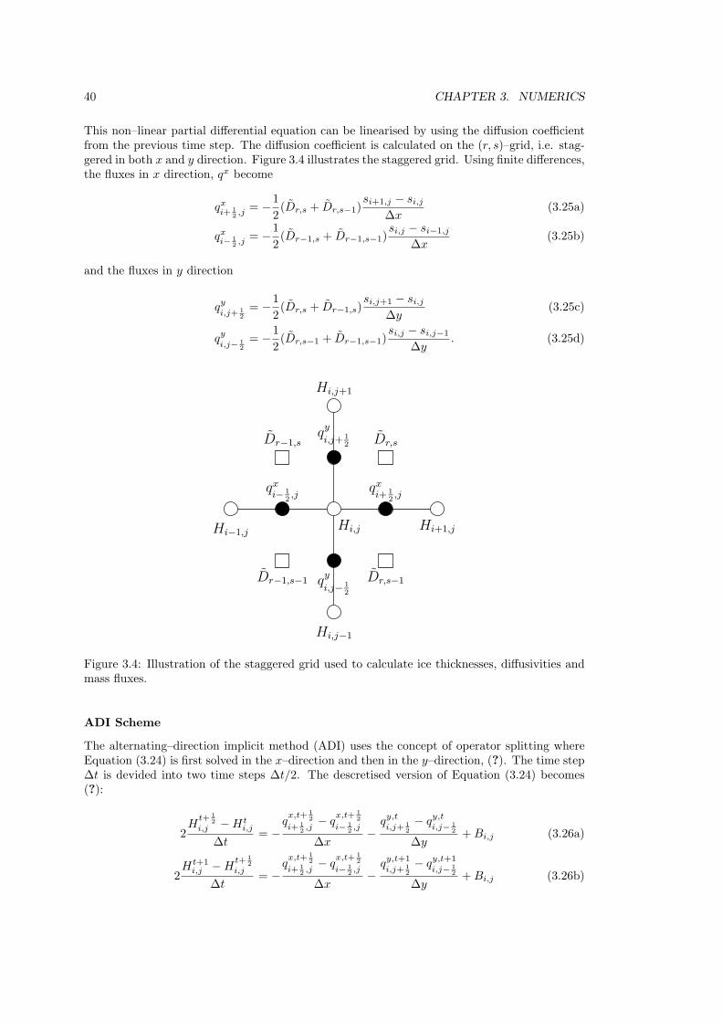
40 CHAPTER 3. NUMERICS
This non–linear partial differential equation can be linearised by using the diffusion coefficientfrom the previous time step. The diffusion coefficient is calculated on the (r, s)–grid, i.e. stag-gered in both x and y direction. Figure 3.4 illustrates the staggered grid. Using finite differences,the fluxes in x direction, qx become
qxi+ 12 ,j
= −1
2(Dr,s + Dr,s−1)
si+1,j − si,j∆x
(3.25a)
qxi− 12 ,j
= −1
2(Dr−1,s + Dr−1,s−1)
si,j − si−1,j
∆x(3.25b)
and the fluxes in y direction
qyi,j+ 1
2
= −1
2(Dr,s + Dr−1,s)
si,j+1 − si,j∆y
(3.25c)
qyi,j− 1
2
= −1
2(Dr,s−1 + Dr−1,s−1)
si,j − si,j−1
∆y. (3.25d)
Hi−1,jHi+1,j
Hi,j+1
Hi,j−1
Hi,j
qxi− 1
2,j
qxi+ 1
2,j
qy
i,j+ 1
2
qy
i,j− 1
2
Dr−1,s−1 Dr,s−1
Dr,sDr−1,s
Figure 3.4: Illustration of the staggered grid used to calculate ice thicknesses, diffusivities andmass fluxes.
ADI Scheme
The alternating–direction implicit method (ADI) uses the concept of operator splitting whereEquation (3.24) is first solved in the x–direction and then in the y–direction, (?). The time step∆t is devided into two time steps ∆t/2. The descretised version of Equation (3.24) becomes(?):
2H
t+ 12
i,j −Hti,j
∆t= −
qx,t+ 1
2
i+ 12 ,j
− qx,t+ 1
2
i− 12 ,j
∆x−
qy,ti,j+ 1
2
− qy,ti,j− 1
2
∆y+Bi,j (3.26a)
2Ht+1
i,j −Ht+ 1
2i,j
∆t= −
qx,t+ 1
2
i+ 12 ,j
− qx,t+ 1
2
i− 12 ,j
∆x−
qy,t+1
i,j+ 12
− qy,t+1
i,j− 12
∆y+Bi,j (3.26b)
3.1. ICE THICKNESS EVOLUTION 41
Gathering all t+ 12 terms on the left side, Equation (3.26a) can be expressed as a tri–diagonal
set of equations for each row j:
−αi,jHt+ 1
2i−1,j + (1− βi,j)H
t+ 12
i,j − γi,jHt+ 1
2i+1,j = δi,j (3.27)
with
αi,j =Dr−1,s + Dr−1,s−1
4∆x2∆t (3.28a)
βi,j = −Dr,s + 2Dr−1,s + Dr−1,s−1
4∆x2∆t = −(αi,j + γi,j) (3.28b)
γi,j =Dr,s + Dr,s−1
4∆x2∆t (3.28c)
and the RHS,
δi,j = Hti,j −
∆t
2∆y
(qy,ti,j+ 1
2
− qy,ti,j− 1
2
)+
∆t
2Bi,j + αi,jhi−1,j − βi,jhi,j + γi,jhi+1,j . (3.28d)
A similar tri–diagonal system is found for each column, i of Equation (3.26b).
Linearised Semi–Implicit Scheme
Using the Crank–Nicolson scheme, the semi–implicit temporal discretisation of (3.24) is then:
Ht+1i,j −Ht
i,j
∆t=
qx,t+1
i+ 12 ,j
− qx,t+1
i− 12 ,j
2∆x+
qy,t+1
i,j+ 12
− qy,t+1
i,j− 12
2∆y
+qx,ti+ 1
2 ,j− qx,t
i− 12 ,j
2∆x+
qy,ti,j+ 1
2
− qy,ti,j− 1
2
2∆y+Bi,j (3.29)
The superscripts t and t+1 indicate at what time the ice thickness H is evaluated. Collecting allHt+1 terms of (3.29) on the LHS and moving all other terms to the RHS we can rewrite (3.29)as
−αi,jHt+1i−1,j − βi,jH
t+1i+1,j − γi,jH
t+1i,j−1 − δi,jH
t+1i,j+1 + (1− εi,j)H
t+1i,j = ζi,j (3.30)
with the RHS,
ζi,j = αi,jHti−1,j + βi,jH
ti+1,j + γi,jH
ti,j−1 + δi,jH
ti,j+1 + (1 + εi,j)H
ti,j
+ 2(αi,jhi−1,j + βi,jhi+1,j + γi,jhi,j−1 + δi,jhi,j+1 + εi,jhi,j) +Bi,j∆t (3.31)
with the elements of the sparse matrix
αi,j =Dr−1,s + Dr−1,s−1
4∆x2∆t (3.32a)
βi,j =Dr,s + Dr,s−1
4∆x2∆t (3.32b)
γi,j =Dr,s−1 + Dr−1,s−1
4∆y2∆t (3.32c)
δi,j =Dr,s + Dr−1,s
4∆y2∆t (3.32d)
εi,j = −(αi,j + βi,j + γi,j + δi,j) (3.32e)
This matrix equation is solved using an iterative matrix solver for non-symmetric sparsematrices. The solver used here is the bi–conjugate gradient method with incomplete LU de-composition preconditioning provided by the SLAP package.
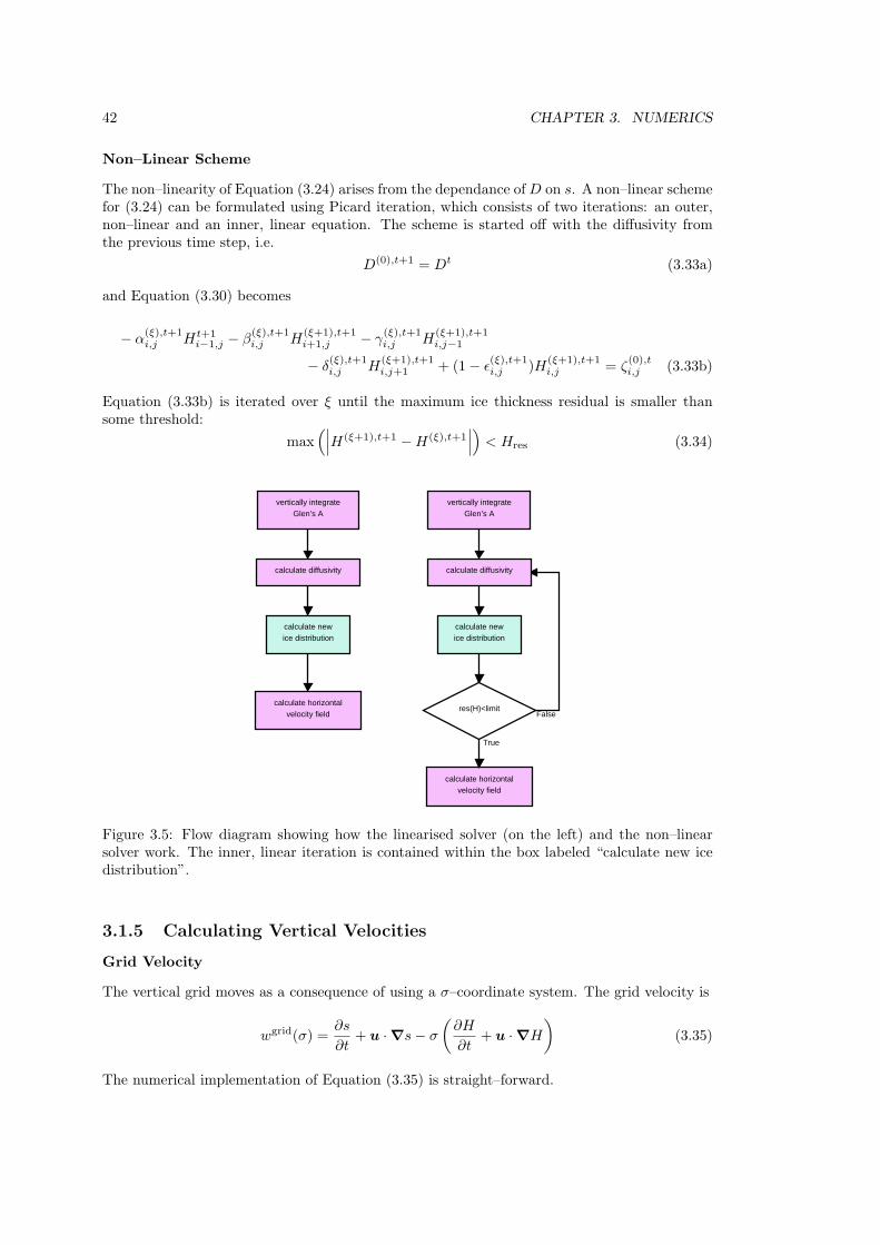
42 CHAPTER 3. NUMERICS
Non–Linear Scheme
The non–linearity of Equation (3.24) arises from the dependance ofD on s. A non–linear schemefor (3.24) can be formulated using Picard iteration, which consists of two iterations: an outer,non–linear and an inner, linear equation. The scheme is started off with the diffusivity fromthe previous time step, i.e.
D(0),t+1 = Dt (3.33a)
and Equation (3.30) becomes
− α(ξ),t+1i,j Ht+1
i−1,j − β(ξ),t+1i,j H
(ξ+1),t+1i+1,j − γ
(ξ),t+1i,j H
(ξ+1),t+1i,j−1
− δ(ξ),t+1i,j H
(ξ+1),t+1i,j+1 + (1− ε
(ξ),t+1i,j )H
(ξ+1),t+1i,j = ζ
(0),ti,j (3.33b)
Equation (3.33b) is iterated over ξ until the maximum ice thickness residual is smaller thansome threshold:
max(∣∣∣H(ξ+1),t+1 −H(ξ),t+1
∣∣∣) < Hres (3.34)
calculate horizontalvelocity field
vertically integrateGlen’s A
vertically integrateGlen’s A
calculate diffusivity calculate diffusivity
calculate newice distribution
calculate newice distribution
calculate horizontalvelocity field
res(H)<limit
True
False
Figure 3.5: Flow diagram showing how the linearised solver (on the left) and the non–linearsolver work. The inner, linear iteration is contained within the box labeled “calculate new icedistribution”.
3.1.5 Calculating Vertical Velocities
Grid Velocity
The vertical grid moves as a consequence of using a σ–coordinate system. The grid velocity is
wgrid(σ) =∂s
∂t+ u ·∇s− σ
(∂H
∂t+ u ·∇H
)(3.35)
The numerical implementation of Equation (3.35) is straight–forward.
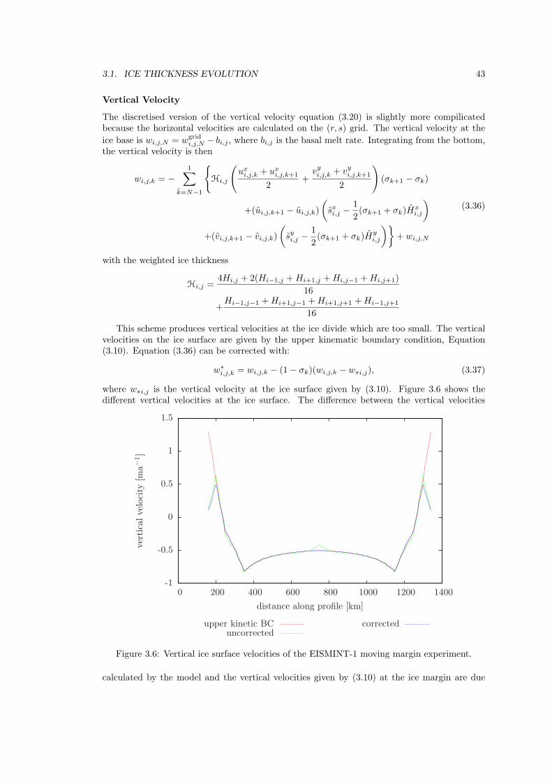
3.1. ICE THICKNESS EVOLUTION 43
Vertical Velocity
The discretised version of the vertical velocity equation (3.20) is slightly more compilicatedbecause the horizontal velocities are calculated on the (r, s) grid. The vertical velocity at the
ice base is wi,j,N = wgridi,j,N − bi,j , where bi,j is the basal melt rate. Integrating from the bottom,
the vertical velocity is then
wi,j,k = −1∑
k=N−1
{Hi,j
(uxi,j,k + ux
i,j,k+1
2+
vyi,j,k + vyi,j,k+1
2
)(σk+1 − σk)
+(ui,j,k+1 − ui,j,k)
(sxi,j −
1
2(σk+1 + σk)H
xi,j
)+(vi,j,k+1 − vi,j,k)
(syi,j −
1
2(σk+1 + σk)H
yi,j
)}+ wi,j,N
(3.36)
with the weighted ice thickness
Hi,j =4Hi,j + 2(Hi−1,j +Hi+1,j +Hi,j−1 +Hi,j+1)
16
+Hi−1,j−1 +Hi+1,j−1 +Hi+1,j+1 +Hi−1,j+1
16
This scheme produces vertical velocities at the ice divide which are too small. The verticalvelocities on the ice surface are given by the upper kinematic boundary condition, Equation(3.10). Equation (3.36) can be corrected with:
w∗i,j,k = wi,j,k − (1− σk)(wi,j,k − wsi,j), (3.37)
where wsi,j is the vertical velocity at the ice surface given by (3.10). Figure 3.6 shows thedifferent vertical velocities at the ice surface. The difference between the vertical velocities
correcteduncorrected
upper kinetic BC
distance along profile [km]
verticalvelocity
[ma−1]
1400120010008006004002000
1.5
1
0.5
0
-0.5
-1
Figure 3.6: Vertical ice surface velocities of the EISMINT-1 moving margin experiment.
calculated by the model and the vertical velocities given by (3.10) at the ice margin are due
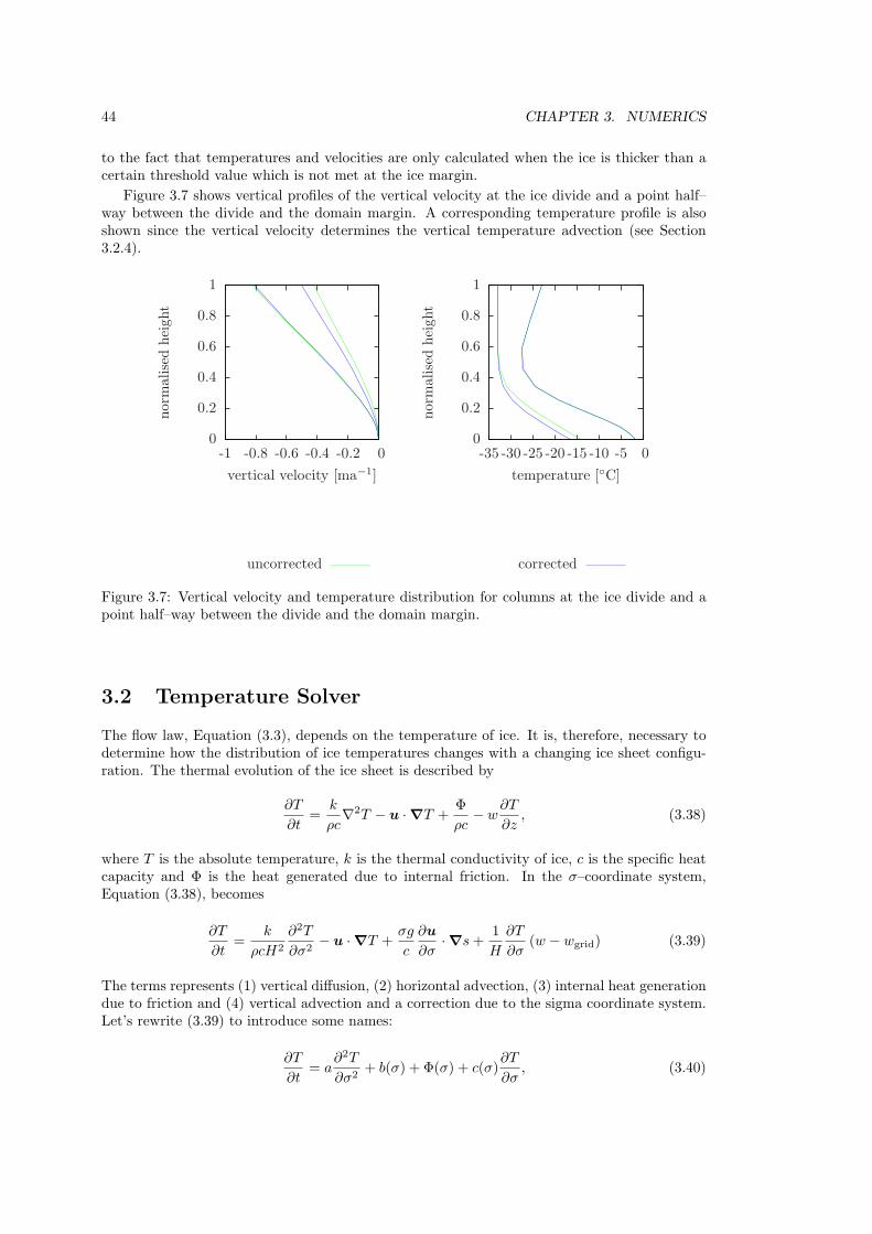
44 CHAPTER 3. NUMERICS
to the fact that temperatures and velocities are only calculated when the ice is thicker than acertain threshold value which is not met at the ice margin.
Figure 3.7 shows vertical profiles of the vertical velocity at the ice divide and a point half–way between the divide and the domain margin. A corresponding temperature profile is alsoshown since the vertical velocity determines the vertical temperature advection (see Section3.2.4).
corrected
temperature [◦C]
norm
alisedheight
0-5-10-15-20-25-30-35
1
0.8
0.6
0.4
0.2
0
uncorrected
vertical velocity [ma−1]
norm
alisedheight
0-0.2-0.4-0.6-0.8-1
1
0.8
0.6
0.4
0.2
0
Figure 3.7: Vertical velocity and temperature distribution for columns at the ice divide and apoint half–way between the divide and the domain margin.
3.2 Temperature Solver
The flow law, Equation (3.3), depends on the temperature of ice. It is, therefore, necessary todetermine how the distribution of ice temperatures changes with a changing ice sheet configu-ration. The thermal evolution of the ice sheet is described by
∂T
∂t=
k
ρc∇2T − u ·∇T +
Φ
ρc− w
∂T
∂z, (3.38)
where T is the absolute temperature, k is the thermal conductivity of ice, c is the specific heatcapacity and Φ is the heat generated due to internal friction. In the σ–coordinate system,Equation (3.38), becomes
∂T
∂t=
k
ρcH2
∂2T
∂σ2− u ·∇T +
σg
c
∂u
∂σ·∇s+
1
H
∂T
∂σ(w − wgrid) (3.39)
The terms represents (1) vertical diffusion, (2) horizontal advection, (3) internal heat generationdue to friction and (4) vertical advection and a correction due to the sigma coordinate system.Let’s rewrite (3.39) to introduce some names:
∂T
∂t= a
∂2T
∂σ2+ b(σ) + Φ(σ) + c(σ)
∂T
∂σ, (3.40)
3.2. TEMPERATURE SOLVER 45
where
a =k
ρcH2(3.41a)
b(σ) = −u ·∇T (3.41b)
Φ(σ) =σg
c
∂u
∂σ·∇s (3.41c)
c(σ) =1
H(w − wgrid) (3.41d)
3.2.1 Vertical Diffusion
Discretisation of ∂2T/∂σ2 is slightly complicated because the vertical grid is irregular. UsingTaylor series the central difference formulas are
∂T
∂σ
∣∣∣∣σk−1/2
=Tk − Tk−1
σk − σk−1(3.42a)
and
∂T
∂σ
∣∣∣∣σk+1/2
=Tk+1 − Tk
σk+1 − σk(3.42b)
The second partial derivative is then, also uning central differences:
∂2T
∂σ2
∣∣∣∣σk
=∂T/∂σ|σk+1/2
− ∂T/∂σ|σk−1/2
1/2 (σk+1 − σk−1)(3.42c)
Inserting (3.42a) and (3.42b) into (3.42c), we get:
=2(Tk+1 − Tk)
(σk+1 − σk)(σk+1 − σk−1)− 2(Tk − Tk−1)
(σk − σk−1)(σk+1 − σk−1)(3.42d)
Finally, the terms of equation (3.42d) are rearranged:
∂2T
∂σ2
∣∣∣∣σk
=2Tk−1
(σk − σk−1)(σk+1 − σk−1)− 2Tk
(σk+1 − σk)(σk − σk−1)
+2Tk+1
(σk+1 − σk)(σk+1 − σk−1)(3.43)
3.2.2 Horizontal Advection
The horizontal advection term, −u ·∇T is solved using an upwinding scheme. Let’s start withthe 1–dimensional case. The method discussed can be straightforwadly extented to 2D. Asalways, the temperature function is expressed as a Taylor series.
T (x+∆x) = T (x) + ∆xT ′(x) +∆x2
2T ′′(x) + . . . (3.44a)
If we subsitute ∆x with 2∆x, Equation (3.44a)
T (x+ 2∆x) = T (x) + 2∆xT ′(x) + 2∆x2T ′′(x) + . . . (3.44b)
46 CHAPTER 3. NUMERICS
From (3.44a) and (3.44b) we can construct a difference formula where the O(∆x2) error iscancelled, by multiplying (3.44a) with 4 and substracting the result from (3.44b):
T ′+(x) =
4T (x+∆x)− T (x+ 2∆x)− 3T (x)
2∆x(3.45a)
and similarly for the backward difference:
T ′−(x) = −4T (x−∆x)− T (x− 2∆x)− 3T (x)
2∆x(3.45b)
So the horizontal advection term in one dimensions becomes:
bx = −ux∂T
∂x=
−ux
2∆x
{−(4Ti−1 − Ti−2 − 3Ti) when ux > 0
4Ti+1 − Ti+2 − 3Ti when ux < 0(3.46)
A similar expression is found for by by simply substituting y for x. Finally, the combinedhorizontal advection term, is simply
b = −u ·∇T = −(ux
∂T
∂x+ uy
∂T
∂y
)= bx + by = b1 + b2Ti (3.47)
3.2.3 Heat Generation
Taking the derivative of (3.18) with respect to σ, we get
∂ux
∂σ= −2(ρg)nHn+1|∇s|n−1 ∂s
∂xA(T ∗)σn (3.48)
Thus,
Φ(σ) =σg
c
∂u
∂σ·∇s =
σg
c
(∂ux
∂σ
∂s
∂x+
∂uy
∂σ
∂s
∂y
)= −2(ρg)nHn+1|∇s|n−1σg
cA(T ∗)σn
((∂s
∂x
)2
+
(∂s
∂y
)2)
= − 2
cρ(gσρ)n+1 (H|∇s|)n+1
A(T ∗)
(3.49)
The constant factor 2cρ (gσρ)
n+1 is calculated during initialisation in the subroutine init temp.This factor is assigned to array c1(1:upn). c1 also includes various scaling factors and the factor1/16 to normalise A.
The next factor, (H|∇s|)n+1is calculated in the subroutine finddisp:
c2i,j =
(Hi,j
√Sx
2
i,j + Sy2
i,j
)n+1
, (3.50)
The final factor is found by averaging over the neighbouring nodes:
Ai,j = 4Ai,j +2(Ai−1,j +Ai+1,j +Ai,j−1+Ai,j+1)+(Ai−1,j−1+Ai+1,j−1+Ai+1,j+1+Ai−1,j+1)(3.51)
3.2.4 Vertical Advection
The vertical advection term, ∂T/∂σ is solved using the central difference formula for unevenlyspaced nodes:
∂T
∂σ=
Tk+1 − Tk−1
σk+1 − σk−1(3.52)
3.2. TEMPERATURE SOLVER 47
3.2.5 Boundary Conditions
At the upper boundary, ice temperatures are set to the surface temperature, Tsurf. The ice atthe base is heated by the geothermal heat flux and sliding friction:
∂T
∂σ
∣∣∣∣σ=1
= −GH
k− Hτ b · u(1)
k, (3.53)
where τ b = −ρgH∇s is the basal shear stress and u(1) is the basal ice velocity. Ice temperaturesare held constant if they reach the pressure melting point of ice, i.e.
T ∗ = Tpmp if T ≥ Tpmp. (3.54)
Excess heat is then used to formulate a melt rate, S:
S =k
ρL
(∂T ∗
∂z− ∂T
∂z
), (3.55)
where L is the specific latent heat of fusion. Finally, basal temperatures are held constant, ifthe ice is floating:
∂T (1)
∂t= 0. (3.56)
3.2.6 Putting it all together
Equation (3.39) is solved for each ice column. The horizontal dependency of the horizontaladvection term, (3.41b), is resolved by iterating the vertical solution. Putting the individualterms together using a fully explicit finite differences scheme, Equation (3.40) becomes
Tk,t+1 − Tk,t
∆t=
(2aTk−1,t
(σk − σk−1)(σk+1 − σk−1)− 2aTk,t
(σk+1 − σk)(σk − σk−1,t)
+2aTk+1,t
(σk+1 − σk)(σk+1 − σk−1)
)+ b1k,t + b2kTk,t +Φk + ck
Tk+1,t − Tk−1,t
σk+1 − σk−1(3.57a)
and similarly the fully implicit scheme
Tk,t+1 − Tk,t
∆t=
(2aTk−1,t+1
(σk − σk−1)(σk+1 − σk−1)− 2aTk,t+1
(σk+1 − σk)(σk − σk−1,t+1)
+2aTk+1,t+1
(σk+1 − σk)(σk+1 − σk−1)
)+ b1k,t+1 + b2kTk,t+1 +Φk + ck
Tk+1,t+1 − Tk−1,t+1
σk+1 − σk−1(3.57b)
Taking the average of Equations (3.57a) and (3.57b) gives the Crank–Nicholson scheme. Theresulting equation is then rearranged and terms of Tk−1,t+1, Tk,t+1 and Tk+1,t+1 are combinedto give the tri–diagonal system
αkTk−1,t+1 + βkTk,t+1 + γkTk+1,t+1 = δk (3.58)
where, for k = 2, N − 1
αk = −1
2
2a∆t
(σk − σk−1)(σk+1 − σk−1)+
1
2
ck∆t
σk+1 − σk−1(3.59a)
βk = 1 +1
2
2a∆t
(σk+1 − σk)(σk − σk−1)− 1
2b2k∆t = 1− αk − γk − 1
2b2k∆t (3.59b)
γk = −1
2
2a∆t
(σk+1 − σk)(σk+1 − σk−1)− 1
2
ck∆t
σk+1 − σk−1(3.59c)
δk = −αkTk−1,t + (2− βk)Tk,t − γkTk+1,t +1
2(b1k,t + b1k,t+1)∆t+Φk∆t (3.59d)
48 CHAPTER 3. NUMERICS
Boundary Conditions
At the upper boundary:
α1 = 0, β1 = 1, γ1 = 0, δ1 = Tsurf (3.59e)
The lower boundary condition is somewhat more complicated. Here we only look at thecase when the temperature is below the pressure melting point of ice. BC for floating ice andtemperatures at the pressure melting point of ice are trivial. The geothermal heat flux is appliedat the lower boundary, i.e. Equation (3.42b) becomes
∂T
∂σ
∣∣∣∣σk+1/2
= −GH
k(3.60)
Assuming that σk − σk−1 = σk+1 − σk = ∆σ and inserting (3.42a) and (3.60) into (3.42c), thesecond partial derivative becomes
∂2T
∂σ2
∣∣∣∣σN
=
(−GH
k− TN − TN−1
∆σ
)/∆σ = − GH
k∆σ− TN − TN−1
∆σ2(3.61)
Inserting the new conduction term and replacing the derivative of the vertical advection termwith the Neuman boundary condition, Equation (3.57a) becomes
TN,t+1 − TN,t
∆t= −a
(GH
k∆σ+
TN,t − TN−1,t
∆σ2
)+ b1N,t + b2NTN,t +ΦN − cN
GH
k(3.62a)
and similarly for Equation (3.57b)
TN,t+1 − TN,t
∆t= −a
(GH
k∆σ+
TN,t+1 − TN−1,t+1
∆σ2
)+ b1N,t+1 + b2NTN,t+1
+ΦN − cNGH
k(3.62b)
The elements of the tri–diagonal system at the lower boundary are then
αN = − a∆t
2(σN − σN−1)2(3.63a)
βN = 1− αN +1
2b2N∆t (3.63b)
γN = 0 (3.63c)
δN =− αNTN−1,t + (2− βN )TN,t − aGH∆t
k(σN − σN−1)
+1
2(b1N,t + b1N,t+1)∆t+ΦN∆t− cN
GH∆t
k
(3.63d)
3.3 Basal Boundary Condition
The Section describes the formulation of the basal boundary condition. An interface for theupper boundary condition (atmospheric BC) is easily defined by the surface temperature andmass balance. Similarly, the basal boundary consists of mechanical and thermal boundaryconditions. The complications arise because the thermal and mechanical boundary conditionsdepend on each other. The interface of the basal boundary can be described with the followingfields (see also Fig.3.8):
1. basal traction: this field specifies a parameter which is used to allow basal sliding.
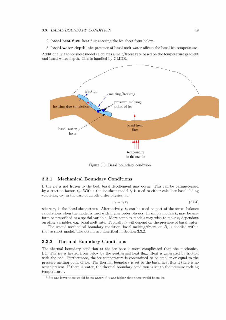
3.3. BASAL BOUNDARY CONDITION 49
2. basal heat flux: heat flux entering the ice sheet from below.
3. basal water depth: the presence of basal melt water affects the basal ice temperature
Additionally, the ice sheet model calculates a melt/freeze rate based on the temperature gradientand basal water depth. This is handled by GLIDE.
temperaturein the mantle
pressure meltingpoint of ice
basal heatfluxbasal water
layer
melting/freezingtraction
heating due to friction
Figure 3.8: Basal boundary condition.
3.3.1 Mechanical Boundary Conditions
If the ice is not frozen to the bed, basal decollement may occur. This can be parameterisedby a traction factor, tb. Within the ice sheet model tb is used to either calculate basal slidingvelocities, ub, in the case of zeroth order physics, i.e.
ub = tbτ b (3.64)
where τb is the basal shear stress. Alternatively, tb can be used as part of the stress–balancecalculations when the model is used with higher order physics. In simple models tb may be uni-form or prescribed as a spatial variable. More complex models may wish to make tb dependanton other variables, e.g. basal melt rate. Typically tb will depend on the presence of basal water.
The second mechanical boundary condition, basal melting/freeze–on B, is handled withinthe ice sheet model. The details are described in Section 3.3.2.
3.3.2 Thermal Boundary Conditions
The thermal boundary condition at the ice base is more complicated than the mechanicalBC. The ice is heated from below by the geothermal heat flux. Heat is generated by frictionwith the bed. Furthermore, the ice temperature is constrained to be smaller or equal to thepressure melting point of ice. The thermal boundary is set to the basal heat flux if there is nowater present. If there is water, the thermal boundary condition is set to the pressure meltingtemperature1.
1if it was lower there would be no water, if it was higher than there would be no ice
50 CHAPTER 3. NUMERICS
Basal Melting and Freezing
At the ice base, z = h, we can define outgoing and incoming heat fluxes, Ho and Hi:
Ho = −kice∂T
∂z
∣∣∣∣z=h+
(3.65a)
and
Hi = −krock∂T
∂z
∣∣∣∣z=h−
+ ub · τ b +
{ρiceB/L when B < 0
0 otherwise(3.65b)
where kice and krock are the thermal conductivities of ice and rock, ub · τ b is the heat generatedby friction with the bed and L is the latent heat of fusion of pure water. The basal melt/freeze–on rate, B can then be calculated from the difference between the incoming and outgoing heatfluxes:
B =Ho −Hi
ρiceL(3.66)
Freeze–on occurs if B is negative, basal melting occurs if B is positive.
Geothermal Heat Flux
The heat flux accross the basal boundary depends on past temperature variations since tem-perature perturbations penetrate the bed rock if the ice is frozen to the ground (?). The heatequation for the bed rock layer is given by the diffusion equation
∂T
∂t=
krockρrockcrock
∇2T =krock
ρrockcrock
(∂2T
∂x2+
∂2T
∂y2+
∂2T
∂z2
), (3.67)
where krock is the thermal conductivity, ρrock the density and crock the specific heat capacity ofthe bed rock layer.
Initial conditions for the temperature field T are found by applying the geothermal heatflux, G to an arbitrary surface temperature T0:
T (x, y, z) = T0 +G
krockz. (3.68)
This ensures that initially the geothermal heat flux experienced by the ice sheet is equal to theregional heat flux. The basal boundary condition of the bedrock layer is kept constant, i.e.
T (x, y,Hrock) = T0 +G
krockHrock. (3.69)
Lateral boundary conditions are given by
∂T
∂x
∣∣∣∣x=0
=∂T
∂x
∣∣∣∣x=Lx
=∂T
∂y
∣∣∣∣y=0
=∂T
∂y
∣∣∣∣y=Ly
= 0. (3.70)
At the upper boundary, the heat flux of the rock layer has to be matched with the heat flux inthe basal ice layer when the ice is frozen to the bed, i.e.
krock∂T
∂z
∣∣∣∣z=−0
= kice∂T
∂z
∣∣∣∣z=+0
. (3.71)
Otherwise the temperature of the top bedrock layer is set to the surface temperature (if thecell has been occupied by ice, but there is no ice present) or the basal ice temperature (if thereis ice). Equation (3.71) is automatically fulfilled if we set the top bedrock temperature to thebasal ice temperature everywhere and then calculate the geothermal heat flux to be used asboundary condition for Equation (3.38).
3.3. BASAL BOUNDARY CONDITION 51
3.3.3 Numerical Solution
The horizontal grid is described in Section 3.1.1. The vertical grid is irregular like the verticalgrid of the ice sheet model. However, it is not scaled. Also for now, I have ignored topographyor isostatic adjustment, i.e. the bedrock layer is assumed to be flat and constant.
The horizontal second derivative in Equation (3.67) becomes using finite–differences
∂2T
∂x2
∣∣∣∣xi,yi,zi
= Txx,i,j,k =Ti+1,j,k − 2Ti,j,k + Ti−1,j,k
∆x(3.72)
and similarly for ∂2T/∂y2. The vertical second derivative ∂2T/∂z2 is similar to Equation (3.43):
∂2T
∂z2
∣∣∣∣xi,yi,zi
= Tzz,i,j,k =2Ti,j,k−1
(zk − zk−1)(zk+1 − zk−1)− 2Ti,j,k
(zk+1 − zk)(zk − zk−1)
+2Ti,j,k+1
(zk+1 − zk)(zk+1 − zk−1)(3.73)
Using the Crank-Nicholson scheme, Equation (3.67) becomes
T t+1i,j,k − T t
i,j,k
∆t= D
{T t+1xx,i,j,k + T t
xx,i,j,k
2+
T t+1yy,i,j,k + T t
yy,i,j,k
2+
T t+1zz,i,j,k + T t
zz,i,j,k
2
}, (3.74)
with D = krock/(ρrockcrock). Equation (3.74) is solved by gathering all T t+1 terms on the LHSand all other terms on the RHS. The index (i, j, k) is linearised using ι = i+(j−1)N+(k−1)NM .The resulting matrix system is solved using the same bi–conjugate gradient solver as for the icethickness evolution.
3.3.4 Basal Hydrology
It is clear from the discussion above that the presence of basal water plays a crucial role inspecifying both the mechanical and thermal boundary conditions. However, the treatment ofbasal water can vary greatly. Basal water is, therefore, left as an unspecified interface. GLIDEdoes provide a simple local water balance model which can be run in the absence of morecomplex models.
3.3.5 Putting It All Together
The basal boundary consists of the individual components described in the previous sections.All components are tightly linked with each other. Figure 3.9 illustrates how the modules arelinked and in what order they are resolved. The order of executions is then:
1. Find the basal heat flux by either solving the equation describing the thermal evolutionof the lithosphere, Eq. (3.67), or by using the geothermal heat flux directly. The upperboundary condition of (3.67) is the same as the lower boundary condition of the thermalevolution of the ice sheet.
2. The lower boundary condition for the thermal evolution of the ice sheet is either given bythe basal heat flux from Step 1 ; or if melt water is present the basal temperature is setto the pressure melting point of ice.
3. Calculate the temperature distribution within the ice sheet given the boundary conditionfound during Step 2 and the atmospheric BC.
4. Calculate a melt/freeze–on rate using Equation (3.66) given the outgoing heat flux calcu-lated during Step 3, friction with the bed (calculated during the previous Step 7 ) and theincoming heat flux from Step 1. Freezing only occurs when there is basal water.
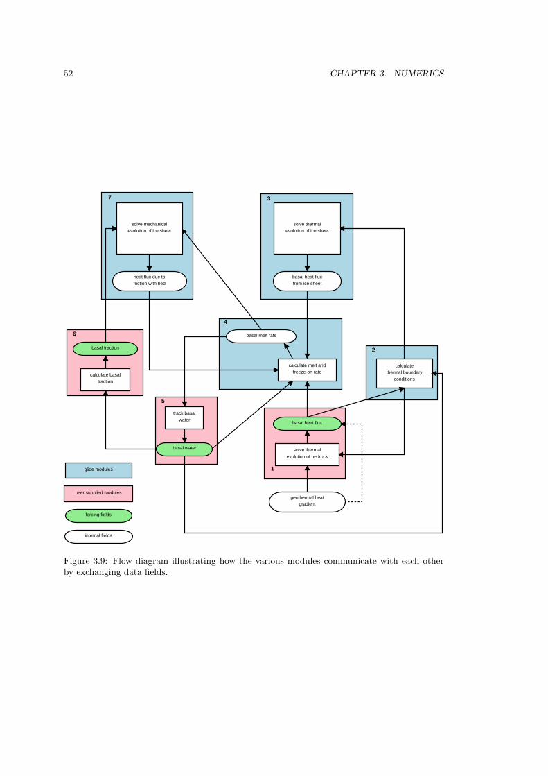
52 CHAPTER 3. NUMERICS
1
2
3
4
5
7
user supplied modules
glide modules
forcing fields
internal fields
6 basal melt rate
calculatethermal boundary
conditionscalculate basal
traction
basal traction
heat flux due tofriction with bed
solve mechanicalevolution of ice sheet
basal water
track basalwater
calculate melt andfreeze-on rate
basal heat fluxfrom ice sheet
solve thermalevolution of ice sheet
basal heat flux
solve thermalevolution of bedrock
geothermal heatgradient
Figure 3.9: Flow diagram illustrating how the various modules communicate with each otherby exchanging data fields.
3.4. ISOSTATIC ADJUSTMENT 53
5. Track basal water. This is a user supplied module which can take any complexity. Inputswill typically be the melt/freeze–on rate determined during Step 4.
6. Calculate the basal traction parameter. Again, this is a user supplied module whichtypically will involve the presence of basal melt water (calculated during Step 5 ).
7. Solve the mechanical ice equations given basal traction parameter from Step 6.
Clearly, this scheme has the problem that heat is lost if the basal heat flux is such that morewater could be frozen than is available. This might be avoided by iterating the process. On theother hand if time steps are fairly small this might no matter to much.
3.4 Isostatic Adjustment
The ice sheet model includes simple approximations for calculating isostatic adjustment. Theseapproximations depend on how the lithosphere and the mantle are treated. For each subsystemthere are two models. The lithosphere can be described as a
local lithosphere: the flexural rigidity of the lithosphere is ignored, i.e. this is equivalent toice floating directly on the asthenosphere;
elastic lithosphere: the flexural rigidity is taken into account;
while the mantle is treated as a
fluid mantle: the mantle behaves like a non-viscous fluid, isostatic equilibrium is reachedinstantaneously;
relaxing mantle: the flow within the mantle is approximated by an exponentially decayinghydrostatic response function, i.e. the mantle is treated as a viscous half space.
3.4.1 Calculation of ice-water load
At each isostasy time-step, the load of ice and water is calculated, as an equivalent mantle-depth(L). If the basal elevation is above sea-level, then the load is simply due to the ice:
L =ρiρm
H, (3.75)
whereH is the ice thickness, with ρi and ρm being the densities of the ice and mantle respectively.In the case where the bedrock is below sea-level, the load is calculated is that due to a change insea-level rise and/or the presence of non-floating ice. When the ice is floating (ρiH < ρo(z0−h)),the load is only due to sea-level changes
L =ρoρm
z0, (3.76)
whereas when the ice is grounded, it displaces the water, and adds an additional load:
L =ρiH + ρoh
ρm. (3.77)
here, ρo is the density of sea water, z0 is the change in sea-level relative to a reference level andh is the bedrock elevation relative to the same reference level. The value of h will be negativefor submerged bedrock, hence the plus sign in (3.77).
54 CHAPTER 3. NUMERICS
3.4.2 Elastic lithosphere model
This is model is selected by setting lithosphere = 1 in the configuration file. By simulatuingthe deformation of the lithosphere, the deformation seen by the aesthenosphere beneath iscalculated. In the absence of this model, the deformation is that due to Archimedes’ Principle,as though the load were floating on the aesthenosphere.
The elastic lithosphere model is based on work by ?, and its implementation is fully describedin ?. The lithosphere model only affects the geometry of the deformation — the timescale forisostatic adjustment is controlled by the aesthenosphere model.
The load due to a single (rectangular) grid point is approximated as being applied to a discof the same area. The deformation due to a disc of ice of radius A and thickness H is given bythese expressions. For r < A:
w(r) =ρiH
ρm
[1 + C1 Ber
(r
Lr
)+ C2 Bei
(r
Lr
)], (3.78)
and for r ≥ A:
w(r) =ρiH
ρm
[D1 Ber
(r
Lr
)+D2 Bei
(r
Lr
)+D3 Ker
(r
Lr
)+D4 Kei
(r
Lr
)], (3.79)
where Ber(x), Bei(x), Ker(x) and Kei(x) are Kelvin functions of zero order, Lr = (D/ρmg))1/4
is the radius of relative stiffness, and D is the flexural rigidity. The constants Ci and Di aregiven by
C1 = aKer′(a)C2 = −aKer′(a)D1 = 0D2 = 0D3 = aBer′(a)D4 = −aBer′(a).
(3.80)
Here, the prime indicates the first spatial derivative of the Kelvin functions.
3.4.3 Relaxing aesthenosphere model
If a fluid mantle is selected, it adjusts instantly to changes in lithospheric loading. However, arelaxing mantle is also available.
Chapter 4
Developer Guide
4.1 Introduction
Everyone with an interest in ice sheet modelling is encouraged to contribute to GLIMMER.However, the structure of the model is complex, and the coding style is more object-orientedthan is generally common in geosciences models. The aim of this chapter is to introduce thesecharacteristics of the model and to suggest some approaches to GLIMMER development. Detailis then provided on some of the modules present within the GLIMMER code base.
In developing new code, several important principles should be borne in mind. These areuseful ideas when developing any code, but are especially important when contributing to anestablished collaborative project like GLIMMER:
• Modularise/objectify. Divide the code up into logically self-contained tasks. In anumerical model of a set of physical processes, this usually means taking each processseparately, though of course the numerical techniques used will have a bearing on how thedivision is done — implicit solutions of systems of equations require a more integratedapproach. Objectification is covered in more detail below.
• Don’t duplicate. At all costs, avoid duplicating code within a model, as it makes bug-fixing and other maintenance nightmarish. Put it in a subroutine and call it from differentplaces. Consider doing this even if the duplicated code is slightly different — write thesubroutine so it will do these different things.
• Don’t reinvent the wheel. If an existing piece of code in the model does what youneed already, use it. If it nearly does what you need, extend it.
• Respect the hierarchy of the code. Some parts of the model are ‘core’, some areshared utility code, some are extensions/drivers/models of boundary conditions. Avoidcreating a birds-nest of dependencies. If a piece of code from an extension acquires generalusefulness, consider moving it to one of the shared utility modules.
• Write for flexibility. The is almost never any justification for using static arrays (i.e.fixed sizes at compile-time), and certainly the size of an array should be defined at only onepoint in the code. Likewise, physical and other numerical parameters should be organisedin a central place, and made configurable at runtime if there is a chance someone mightwant to change them. Think beyond what you’re doing now to what you might want todo in the future, and write code accordingly.
• Be conservative. Although radical restructuring or rewriting can sometimes be nec-essary, it should only be done after careful consideration of the potential consequences.
55
56 CHAPTER 4. DEVELOPER GUIDE
Usually, incremental, gradual change is best. Also, when making changes, it’s very impor-tant to retain the existing functionality and the form of the user interfaces (code interfacesand configuration options) if at all possible. Extend rather than alter.
• Write comments. It’s almost impossible to write too many comments in your code. It’sespecially important to document subroutine arguments, including the units of quantities,temporal validity, etc. Remember, in a few weeks’ time, you’ll probably have forgottenhalf of it, and will be glad of the comments. . .
• Lay out your code neatly. Indentation of code blocks and leaving blank lines betweendifferent sections of code are important ways to make code more readable. Most goodeditors have an automatic indentation facility — Emacs is a good editor in this respect1.
• Use long, meaningful names. There’s not much virtue these days in making variableand subroutine names short and opaque — we don’t have issues with memory, and Fortran90/95 allows names to be up to 31 characters. It may involve a bit more typing to uselong names, and care must be taken to ensure they don’t get too long, but the extra timespent typing is worth it if the code actually means something when you look at it againa few weeks later.
• Use version control. Although it takes a little time to learn to use a version controlsystem, it really does make life easier. If you’ve ever got confused about which version ofthe code you or your collaborators have, or wished you could revert the changes you’ve justmade, then you need version control. We use CVS for GLIMMER, but other systems areavailable. Of these, Subversion is generally seen as a promising alternative and successorto CVS.
The sections that follow cover some of these topics in more detail, but much that passes forgood-practice in code development is best learnt from experience, and by looking at existingcode.
4.2 Introduction to GLIMMER programming techniques
Although GLIMMER is written in Fortran, a very widely used language in the geosciences,many of the techniques employed in the model will be unfamiliar to even seasoned Fortranprogrammers. What follows is a brief description of some of these more advanced techniques.For further information about the topics covered, the reader is directed to ? and ?.
4.2.1 Fortran Modules
Module definition
The basic building block of the GLIMMER structure is the Fortran 90/95 module, which isa way of collecting together subroutines, functions type definitions and variables into a singlescope2. The module may then be used within another piece of code, so that the names in themodules scope are available in the other piece of code. A module block is defined like this:
module module-name
module variable declarations
1Hint: if emacs doesn’t enter the F90 edit mode immediately upon opening a file, you need to type Alt-x,followed by f90-mode, and press <enter>.
2A scope or namespace is the term for the program unit where a given name, such as a variable or subroutinename, is valid. For instance, if a variable is declared at the beginning of a subroutine, the body of the subroutineis that variable’s scope; outside the scope, the name is undefined, or may be defined differently.
4.2. INTRODUCTION TO GLIMMER PROGRAMMING TECHNIQUES 57
derived-type definitions
contains
function and subroutine declarations
end module
The contains is omitted if no subroutines or functions are present. It is good practice to puteach module in a separate file, and give the filename the same name as the module.
Using modules
A module is accessed by another piece of code with the use statement. Thus, if the module foocontains the subroutine bar, another piece of code may make use of it in this way:
program program-name
use foo
implicit none
variable declarations
call bar
end program program-name
Of course, subroutines, functions and modules can all contain use statements as well.
Privacy in modules
By default, all the names in a module’s scope become available to any program element thatreferences it with a use statement. There are circumstances where this is undesirable, and soFortran 90/95 provides a way to define names as public or private. The public and private
statements may both be present in the first block of a module (i.e. before the contains, ifpresent). The list of variable and/or subroutine names follows. For example:
private :: foo, bar, blah
It is good practice to be clear about what parts of a module form a public interface, and definethis formally. A good way of doing this is to set the default to private, and then set specificnames as public:
private
public :: foo, bar
This technique is useful for avoiding name conflicts when two modules might define inter-nal variables or subroutines with the same name (e.g. pi for the value of π). Also, publicsubroutines are best named in an un-generic way, by prefixing their names with the nameof the module. For instance, the module glimmer daily pdd contains the public subroutinesglimmer daily pdd init and glimmer daily pdd mbal.
58 CHAPTER 4. DEVELOPER GUIDE
4.2.2 Derived types
A derived type is a way of collecting together an arbitrary set of variables and arrays into acomposite variable type, instances of which can be addressed with a single name. The conceptof derived types takes us some way towards so-called object-oriented programming (OOP) tech-niques, though there are some important OOP techniques that are not implemented in Fortran90/95.
A derived type is defined in this kind of way:
type typename
real :: realvar
integer :: intvar
real,pointer,dimension(:,:) :: realarr => null()
end type typename
So, a derived type can contain any scalar variables, and also pointers (either scalar pointers orarray pointers). Fortran 90/95 does not permit derived type elements to be allocatable arrays,but since the behaviour of pointer arrays is very similar, this isn’t a serious problem.
The type definition doesn’t actually create any variables though. To do that, you need touse the type declaration to create an instance of the derived type (known as a structure), justas with any other type of variable:
type(typename) :: fred, jim, bob
This creates three structures of type typename, called fred, jim and bob. Structures can behandled like ordinary variables, and passed to subroutines in argument lists, etc. The individualelements may be addressed using the % operator:
fred%realvar = 4.5
jim%intvar = fred%intvar + 7
allocate(bob%realarr(nx,ny))
Note that by default, mathematical operators have no meaning when applied to derivedtypes; writing bob = fred + jim isn’t allowed. If you want to add the elements of fred to theelements of jim, it’s necessary to write a function to do so, so that you would, for example,write bob = typename add(fred,jim) It is possible to define the meaning of the + operator sothat it uses the function typename add to perform the addition (a process known as operatoroverloading), but describing how is beyond the scope of this document. In any case, derivedtypes in GLIMMER are not generally used in a way such that arithmetic operations wouldmake sense.
Usually, derived type definitions are put into modules (before contains), so that they caneasily be used in different pieces of code. The power that this combination of type definitionsand modules gives is described in the next section.
4.2.3 Object-orientation with modules and derived types
As the name implies, the object is the central concept of object-oriented programming. Intraditional OOP terminology, a class defines a type of object. The class has particular attributes,which might be numerical values, strings or whatever (i.e. they’re variables that are part of theclass), and methods, which are things you can ask an object to do to itself (i.e. methods arefunctions or subroutines which are part of a class).
Explaining OOP with examples is notoriously tricky because the easiest examples of classesare those that mirror classes of objects in the real world, but this inevitably seems a bit contrived.So, although it seems a bit ridiculous, here’s one such example. . . Imagine a class which describesa domestic oven. What are the attributes of an oven, that differentiate one oven from another?These could be the size of the oven, it’s type (electric or gas), as well those things that describe
4.2. INTRODUCTION TO GLIMMER PROGRAMMING TECHNIQUES 59
its present state: the thermostat setting, the actual oven temperature, whether the heatingelement is on or off, and whether the door is open or not
Secondly, what kind of actions can we perform on the oven? Most likely, we want to be ableto open and close the oven door, check the present temperature, and set the thermostat. Theseactions are the methods.
In terms of Fortran 90, we can use the mechanism of modules and derived types to implementa somewhat limited form of OOP:
module domestic_oven
type oven
real :: width,height,depth
real :: thermostat
real :: temperature
logical :: element ! .true. for no, .false. for off
logical :: door ! .true. for open, .false. for closed
character(10) :: oven_type
end type oven
contains
subroutine oven_set_thermostat(self,temp)
type(oven) :: self
real :: temp
self%temperature = temp
end subroutine oven_set_thermostat
. . . plus other functions/subroutines
end module domestic_oven
A module like this will usually include a subroutine to initialise objects; in this case, you wouldexpect to be able to specify the size of the oven, its type, initial temperature, etc.
So much for computer models of domestic ovens; what use is OOP to ice modellers? Well,using the technique described above is what allows GLIMMER to be used to run several regionalice models simultaneously. It also makes adding new mass-balance models to GLINT mucheasier. In fact, the principles of OOP are used all over the GLIMMER code, so it is worthgetting to grips with them.
4.2.4 Example of OOP in Glimmer
A good, self-contained example of GLIMMER programming style, and the use of OOP is the waythat the daily PDD mass-balance scheme (in glimmer daily pdd.F90) has been implemented.Here, the parameters of the scheme are stored in the derived type glimmer daily pdd params,and the public interface of the module is limited to this derived type, and two subroutines(glimmer daily pdd init and glimmer daily pdd mbal). Everything else is kept private withinthe module. The initialisation subroutine uses the standard GLIMMER configuration file readerto get input parameters, and the GLIMMER logging mechanism to output data to the screenand/or file. The object-like structure means that it is easy to use the daily PDD model withinsome other piece of code: all one needs to do is declare an instance of glimmer daily pdd params,initialise it appropriately, and then call the glimmer daily pdd mbal subroutine. Also, although
60 CHAPTER 4. DEVELOPER GUIDE
the PDD model is currently initialised from file, it would be easy to write an alternative ini-tialisation routine within the module to get the parameters from a subroutine argument list,extending the capabilities of the module rather than changing the present interface.
4.2.5 Pointers
The final more advanced topic covered here is the Fortran pointer. Thankfully, the name isself-explanatory — a pointer is a thing that points to another thing. This might not sound likemuch use, but since pointers can be made to point at different things as the program runs, andcan have memory allocated for them to point to, they can be used to create flexible, dynamicdata structures. The thing that a pointer points to is called a target.
Pointer basics
Pointers are declared much like an ordinary variable, but with the pointer attribute. Forexample, to declare an integer pointer, one would write this:
integer, pointer :: foo => null()
The second part of this statement (=>null()) initialises the pointer to null (i.e. pointing tonothing). This is only available in Fortran 95, but it is highly desirable to use it, as otherwisethe pointer’s target is undefined3.
Note that although we have declared a pointer with this statement, we can’t use it as avariable yet, as it isn’t pointing at an integer-sized chunk of memory. There are two waysof rectifying this: either the pointer can be made to point to an existing variable, or a newblock of memory can be allocated to hold the target. These two methods are known as pointerassignment and pointer allocation, respectively.
Pointer assignment
Pointing a pointer at something is very simple. The pointer assignment statement uses the =>
operator:
a => b
This statement sets pointer a to point to target b. For this to be valid Fortran, a must havethe pointer attribute, while b must be either a variable with the target attribute, or anotherpointer. If the target is a pointer, then the first pointer is set to point at the second pointer’starget. This means that
a => b
c => a
is equivalent to
a => b
c => b
Pointer allocation
A pointer can be made to point to a newly-allocated chunk of memory using the allocate
statement, in the same way as an allocatable array is handled:
allocate(a)
3Undefined is not the same thing as pointing at nothing. Undefined pointers can cause a program to crashvery easily; the lack of null initialisation in Fortran 90 is one of the more serious omissions that Fortran 95 soughtto address.

4.2. INTRODUCTION TO GLIMMER PROGRAMMING TECHNIQUES 61
By using the pointer assignment described above, other pointers may be made to point at thesame piece of memory:
b => a
Un-pointing pointers, and avoiding memory leaks.
A pointer can be nullified (made to point to nothing) in two ways: using the null function, orthe nullify statement:
p => null()
nullify(p)
Care has to be taken with this, however. Recall the memory allocation example given above:
allocate(a)
b => a
It is significant that the memory location that a and b now point to doesn’t have a name of itsown, which means that if a and b are subsequently both made to point to something else, orto nothing, the target variable becomes impossible to recover. Consider this sequence of twostatements:
allocate(a)
a => null()
Here, a block of memory is allocated, and a is made to point to it. Then, a is made to point tonothing. However, the block of memory allocated in the first statement hasn’t been deallocated,and is now unrecoverable — and unusable — since we don’t have a name to refer to it by. Thisis known as a memory leak, and it is a Bad Thing. It’s not disastrous if a few integer-sizedblocks of memory suffer this fate, but if large amounts of memory are lost like this, it is quitepossible for the program to crash or become very slow as a result.
The proper way to avoid memory leaks is to deallocate memory before it becomes derefer-enced, using the deallocate statement4:
allocate(a)
deallocate(a)
a => null()
The reason that this isn’t done automatically when a pointer is nullified is because there may beother pointers still pointing to that memory location. The process of working out which chunksof memory have been ‘orphaned’ and so need to be deallocated (known as garbage collection)is complex, and compiled languages like Fortran don’t usually do it automatically. Avoidingmemory leaks therefore depends on careful program design.
Linked lists
A major use for pointers is the linked list, a flexible data structure whose size and structure canbe changed dynamically, without having to reallocate it from scratch (which is the case withallocatable arrays).
The principle of the linked list is that each element of the list points to the next element.Extra elements can be added to the end of the list by allocating more memory, and making thefinal element point to it. Other actions can be done by manipulating the pointers of the variouselements.
A typical linked list might use the following derived type:
4It’s not clear to me whether the assignment of a to null is necessary in this example. Some compilers takeit as read that if a block of memory that a pointer points to is deallocated, that pointer is also nullified, but Iam not sure if this is universal.
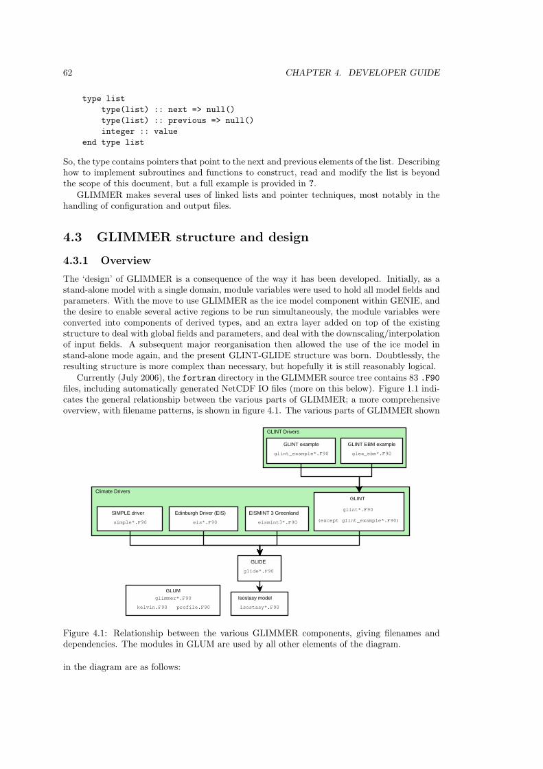
62 CHAPTER 4. DEVELOPER GUIDE
type list
type(list) :: next => null()
type(list) :: previous => null()
integer :: value
end type list
So, the type contains pointers that point to the next and previous elements of the list. Describinghow to implement subroutines and functions to construct, read and modify the list is beyondthe scope of this document, but a full example is provided in ?.
GLIMMER makes several uses of linked lists and pointer techniques, most notably in thehandling of configuration and output files.
4.3 GLIMMER structure and design
4.3.1 Overview
The ‘design’ of GLIMMER is a consequence of the way it has been developed. Initially, as astand-alone model with a single domain, module variables were used to hold all model fields andparameters. With the move to use GLIMMER as the ice model component within GENIE, andthe desire to enable several active regions to be run simultaneously, the module variables wereconverted into components of derived types, and an extra layer added on top of the existingstructure to deal with global fields and parameters, and deal with the downscaling/interpolationof input fields. A subsequent major reorganisation then allowed the use of the ice model instand-alone mode again, and the present GLINT-GLIDE structure was born. Doubtlessly, theresulting structure is more complex than necessary, but hopefully it is still reasonably logical.
Currently (July 2006), the fortran directory in the GLIMMER source tree contains 83 .F90files, including automatically generated NetCDF IO files (more on this below). Figure 1.1 indi-cates the general relationship between the various parts of GLIMMER; a more comprehensiveoverview, with filename patterns, is shown in figure 4.1. The various parts of GLIMMER shown
GLINT Drivers
Climate Drivers
GLIDE
glide*.F90
Isostasy model
isostasy*.F90
GLUMglimmer*.F90
kelvin.F90 profile.F90
Edinburgh Driver (EIS)
eis*.F90
EISMINT 3 Greenland
eismint3*.F90
GLINT
glint*.F90
(except glint_example*.F90)
SIMPLE driver
simple*.F90
GLINT example
glint_example*.F90
GLINT EBM example
glex_ebm*.F90
Figure 4.1: Relationship between the various GLIMMER components, giving filenames anddependencies. The modules in GLUM are used by all other elements of the diagram.
in the diagram are as follows:
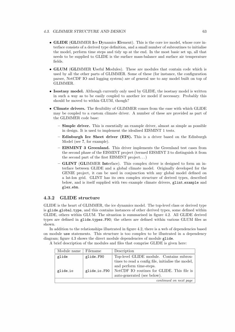
4.3. GLIMMER STRUCTURE AND DESIGN 63
• GLIDE (GLIMMER Ice Dynamics Element). This is the core ice model, whose core in-terface consists of a derived type definition, and a small number of subroutines to initialisethe model, perform time steps and tidy up at the end. In the most basic set up, all thatneeds to be supplied to GLIDE is the surface mass-balance and surface air temperaturefields.
• GLUM (GLIMMER Useful Modules). These are modules that contain code which isused by all the other parts of GLIMMER. Some of these (for instance, the configurationparser, NetCDF IO and logging system) are of general use to any model built on top ofGLIMMER.
• Isostasy model. Although currently only used by GLIDE, the isostasy model is writtenin such a way as to be easily coupled to another ice model if necessary. Probably thisshould be moved to within GLUM, though?
• Climate drivers. The flexibility of GLIMMER comes from the ease with which GLIDEmay be coupled to a custom climate driver. A number of these are provided as part ofthe GLIMMER code base:
– Simple driver. This is essentially an example driver, almost as simple as possiblein design. It is used to implement the idealised EISMINT 1 tests.
– Edinburgh Ice Sheet driver (EIS). This is a driver based on the EdinburghModel (see ?, for example).
– EISMINT 3 Greenland. This driver implements the Greenland test cases fromthe second phase of the EISMINT project (termed EISMINT 3 to distinguish it fromthe second part of the first EISMINT project. . . )
– GLINT (GLIMMER Interface). This complex driver is designed to form an in-terface between GLIDE and a global climate model. Originally developed for theGENIE project, it can be used in conjunction with any global model defined ona lat-lon grid. GLINT has its own complex structure of derived types, describedbelow, and is itself supplied with two example climate drivers, glint example andglex ebm.
4.3.2 GLIDE structure
GLIDE is the heart of GLIMMER, the ice dynamics model. The top-level class or derived typeis glide global type, and this contains instances of other derived types, some defined withinGLIDE, others within GLUM. The situation is summarised in figure 4.2. All GLIDE derivedtypes are defined in glide types.F90; the others are defined within various GLUM files asshown.
In addition to the relationships illustrated in figure 4.2, there is a web of dependencies basedon module use statements. This structure is too complex to be illustrated in a dependencydiagram; figure 4.3 shows the direct module dependencies of module glide.
A brief description of the modules and files that comprise GLIDE is given here:
Module name Filename Description
glide glide.F90 Top-level GLIDE module. Contains subrou-tines to read a config file, initialise the model,and perform time-steps.
glide io glide io.F90 NetCDF IO routines for GLIDE. This file isauto-generated (see below).
continued on next page
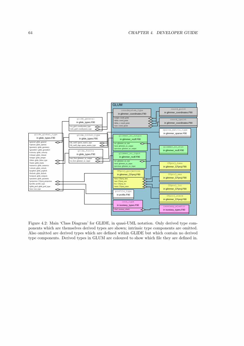
64 CHAPTER 4. DEVELOPER GUIDE
GLUM
glide_global_type
in glide_types.F90
+general: glide_general
+options: glide_options
+geometry: glide_geometry
+geomderv: glide_geomderv
+velocity: glide_velocity
+climate: glide_climate
+temper: glide_temper
+lithot: glide_lithot_type
+funits: glide_funits
+numerics: glide_numerics
+velowk: glide_velowk
+pcgdwk: glide_pcgdwk
+thckwk: glide_thckwk
+tempwk: glide_tempwk
+paramets: glide_paramets
+projection: CFproj_projection
+profile: profile_type
+glide_prof: glide_prof_type
+isos: isos_type
glide_lithot_type
in glide_types.F90
+fd_coeff: sparse_matrix_type
+fd_coeff_slap: sparse_matrix_type
CFproj_projection
in glimmer_CFproj.F90
+laea: CFproj_laea
+aea: CFproj_aea
+lcc: CFproj_lcc
+stere: CFproj_stere
glide_funits
in glide_types.F90
+out_first: glimmer_nc_output
+in_first: glimmer_nc_input
glide_general
in glide_types.F90
+ice_grid: coordsystem_type
+velo_grid: coordsystem_type
profile_type
in profile.F90
isos_type
in isostasy_types.F90
+rbel: isostasy_elastic
isostasy_elastic
in isostasy_types.F90
CFproj_laea
in glimmer_CFproj.F90
CFproj_aea
in glimmer_CFproj.F90
CFproj_lcc
in glimmer_CFproj.F90
CFproj_stere
in glimmer_CFproj.F90
glimmer_nc_input
in glimmer_ncdf.F90
+nc: glimmer_nc_stat
+next: glimmer_nc_input
+previous: glimmer_nc_input
glimmer_nc_output
in glimmer_ncdf.F90
+nc: glimmer_nc_stat
+next: glimmer_nc_output
+previous: glimmer_nc_outputglimmer_nc_stat
in glimmer_ncdf.F90
sparse_matrix_type
in glimmer_sparse.F90
coordsystem_type
in glimmer_coordinates.F90
+origin: coord_point
+delta: coord_point
+delta_r: coord_point
+size: coord_ipoint
coord_point
in glimmer_coordinates.F90
coord_ipoint
in glimmer_coordinates.F90
Figure 4.2: Main ‘Class Diagram’ for GLIDE, in quasi-UML notation. Only derived type com-ponents which are themselves derived types are shown; intrinsic type components are omitted.Also omitted are derived types which are defined within GLIDE but which contain no derivedtype components. Derived types in GLUM are coloured to show which file they are defined in.
4.3. GLIMMER STRUCTURE AND DESIGN 65
module glide
in file glide.F90
module glide_types
in file glide_types.F90
module glide_stop
in file glide_stop.F90
module glide_nc_custom
in file glide_nc_custom.F90
module glide_io
in file glide_io.F90
module glide_lithot
in file glide_lithot.F90
module glide_profile
in file glide_profile.F90
module glide_temp
in file glide_temp.F90
module glide_thck
in file glide_thck.F90
module glide_velo
in file glide_velo.F90
module glide_mask
in file glide_mask.F90
module glide_setup
in file glide_setup.F90
module glimmer_ncparams
in file glimmer_ncparms.F90
module glimmer_config
in file glimmer_config.F90
module glimmer_ncio
in file glimmer_ncio.F90
module glimmer_scales
in file glimmer_ncdf.F90
module glimmer_log
in file glimmer_log.F90
GLUM
module glimmer_global
in file glimmer_global.F90
Figure 4.3: Direct module dependency diagram for module glide only, illustrating the com-plexity of module dependencies.
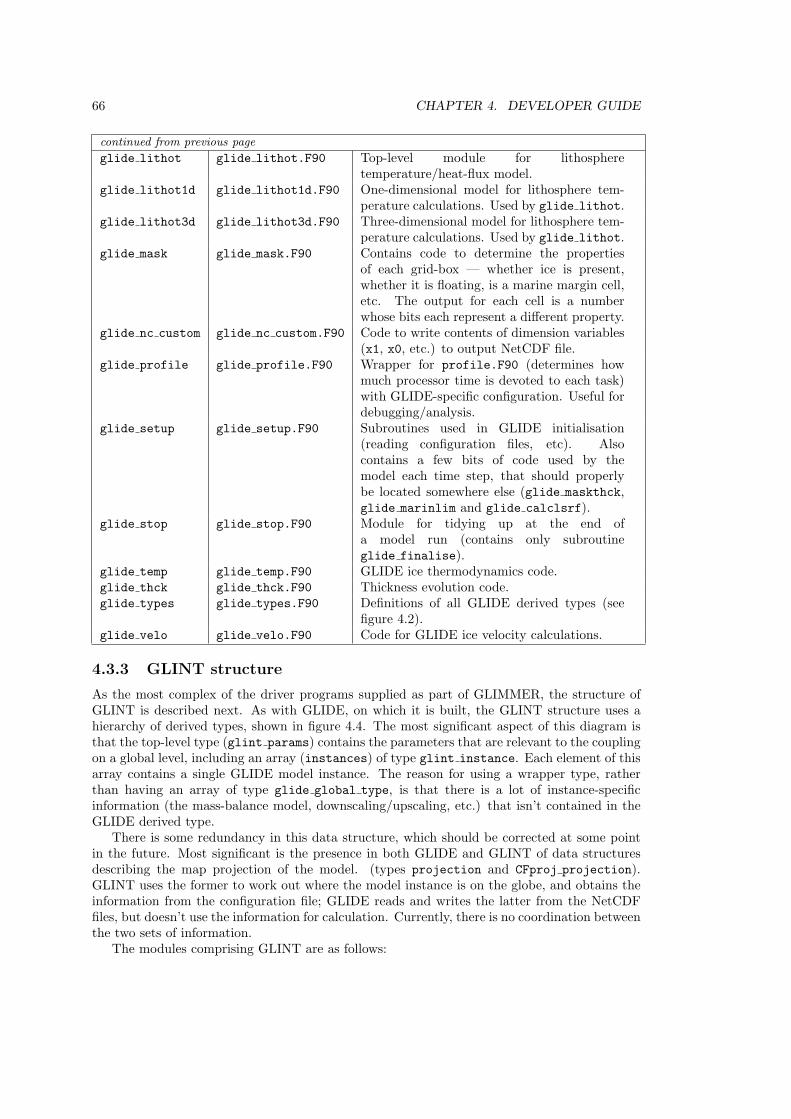
66 CHAPTER 4. DEVELOPER GUIDE
continued from previous page
glide lithot glide lithot.F90 Top-level module for lithospheretemperature/heat-flux model.
glide lithot1d glide lithot1d.F90 One-dimensional model for lithosphere tem-perature calculations. Used by glide lithot.
glide lithot3d glide lithot3d.F90 Three-dimensional model for lithosphere tem-perature calculations. Used by glide lithot.
glide mask glide mask.F90 Contains code to determine the propertiesof each grid-box — whether ice is present,whether it is floating, is a marine margin cell,etc. The output for each cell is a numberwhose bits each represent a different property.
glide nc custom glide nc custom.F90 Code to write contents of dimension variables(x1, x0, etc.) to output NetCDF file.
glide profile glide profile.F90 Wrapper for profile.F90 (determines howmuch processor time is devoted to each task)with GLIDE-specific configuration. Useful fordebugging/analysis.
glide setup glide setup.F90 Subroutines used in GLIDE initialisation(reading configuration files, etc). Alsocontains a few bits of code used by themodel each time step, that should properlybe located somewhere else (glide maskthck,glide marinlim and glide calclsrf).
glide stop glide stop.F90 Module for tidying up at the end ofa model run (contains only subroutineglide finalise).
glide temp glide temp.F90 GLIDE ice thermodynamics code.glide thck glide thck.F90 Thickness evolution code.glide types glide types.F90 Definitions of all GLIDE derived types (see
figure 4.2).glide velo glide velo.F90 Code for GLIDE ice velocity calculations.
4.3.3 GLINT structure
As the most complex of the driver programs supplied as part of GLIMMER, the structure ofGLINT is described next. As with GLIDE, on which it is built, the GLINT structure uses ahierarchy of derived types, shown in figure 4.4. The most significant aspect of this diagram isthat the top-level type (glint params) contains the parameters that are relevant to the couplingon a global level, including an array (instances) of type glint instance. Each element of thisarray contains a single GLIDE model instance. The reason for using a wrapper type, ratherthan having an array of type glide global type, is that there is a lot of instance-specificinformation (the mass-balance model, downscaling/upscaling, etc.) that isn’t contained in theGLIDE derived type.
There is some redundancy in this data structure, which should be corrected at some pointin the future. Most significant is the presence in both GLIDE and GLINT of data structuresdescribing the map projection of the model. (types projection and CFproj projection).GLINT uses the former to work out where the model instance is on the globe, and obtains theinformation from the configuration file; GLIDE reads and writes the latter from the NetCDFfiles, but doesn’t use the information for calculation. Currently, there is no coordination betweenthe two sets of information.
The modules comprising GLINT are as follows:
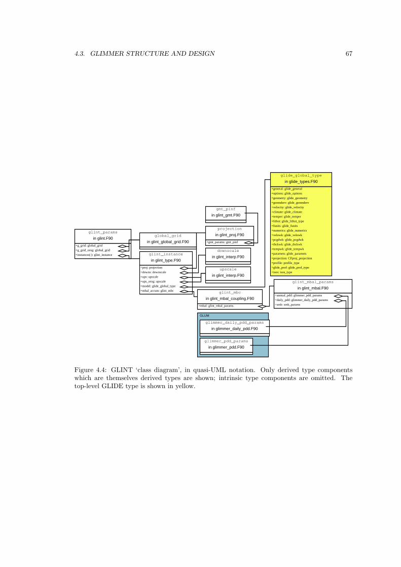
4.3. GLIMMER STRUCTURE AND DESIGN 67
glide_global_type
in glide_types.F90
+general: glide_general
+options: glide_options
+geometry: glide_geometry
+geomderv: glide_geomderv
+velocity: glide_velocity
+climate: glide_climate
+temper: glide_temper
+lithot: glide_lithot_type
+funits: glide_funits
+numerics: glide_numerics
+velowk: glide_velowk
+pcgdwk: glide_pcgdwk
+thckwk: glide_thckwk
+tempwk: glide_tempwk
+paramets: glide_paramets
+projection: CFproj_projection
+profile: profile_type
+glide_prof: glide_prof_type
+isos: isos_type
glint_params
in glint.F90
+g_grid: global_grid
+g_grid_orog: global_grid
+instances(:): glint_instance
global_grid
in glint_global_grid.F90
glint_instance
in glint_type.F90
+proj: projection
+downs: downscale
+ups: upscale
+ups_orog: upscale
+model: glide_global_type
+mbal_accum: glint_mbc
projection
in glint_proj.F90
+gmt_params: gmt_pinf
gmt_pinf
in glint_gmt.F90
downscale
in glint_interp.F90
upscale
in glint_interp.F90
glint_mbal_params
in glint_mbal.F90
+annual_pdd: glimmer_pdd_params
+daily_pdd: glimmer_daily_pdd_params
+smb: smb_params
glint_mbc
in glint_mbal_coupling.F90
+mbal: glint_mbal_params
glimmer_pdd_params
in glimmer_pdd.F90
glimmer_daily_pdd_params
in glimmer_daily_pdd.F90
GLUM
Figure 4.4: GLINT ‘class diagram’, in quasi-UML notation. Only derived type componentswhich are themselves derived types are shown; intrinsic type components are omitted. Thetop-level GLIDE type is shown in yellow.
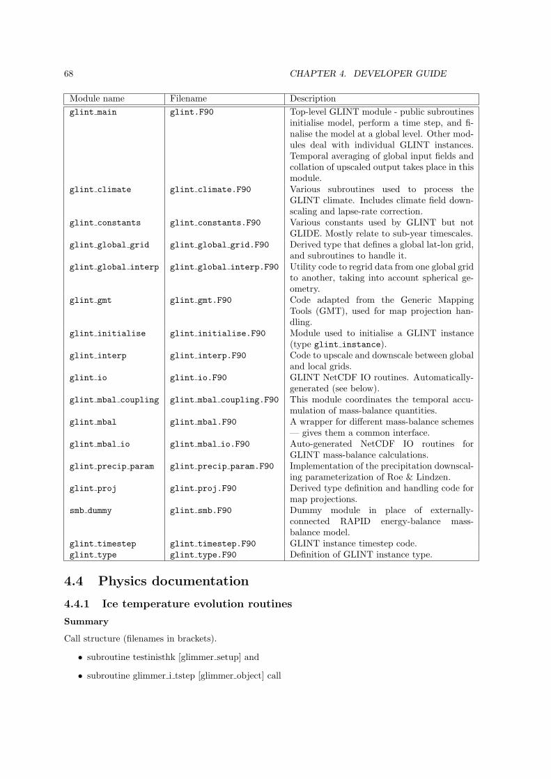
68 CHAPTER 4. DEVELOPER GUIDE
Module name Filename Description
glint main glint.F90 Top-level GLINT module - public subroutinesinitialise model, perform a time step, and fi-nalise the model at a global level. Other mod-ules deal with individual GLINT instances.Temporal averaging of global input fields andcollation of upscaled output takes place in thismodule.
glint climate glint climate.F90 Various subroutines used to process theGLINT climate. Includes climate field down-scaling and lapse-rate correction.
glint constants glint constants.F90 Various constants used by GLINT but notGLIDE. Mostly relate to sub-year timescales.
glint global grid glint global grid.F90 Derived type that defines a global lat-lon grid,and subroutines to handle it.
glint global interp glint global interp.F90 Utility code to regrid data from one global gridto another, taking into account spherical ge-ometry.
glint gmt glint gmt.F90 Code adapted from the Generic MappingTools (GMT), used for map projection han-dling.
glint initialise glint initialise.F90 Module used to initialise a GLINT instance(type glint instance).
glint interp glint interp.F90 Code to upscale and downscale between globaland local grids.
glint io glint io.F90 GLINT NetCDF IO routines. Automatically-generated (see below).
glint mbal coupling glint mbal coupling.F90 This module coordinates the temporal accu-mulation of mass-balance quantities.
glint mbal glint mbal.F90 A wrapper for different mass-balance schemes— gives them a common interface.
glint mbal io glint mbal io.F90 Auto-generated NetCDF IO routines forGLINT mass-balance calculations.
glint precip param glint precip param.F90 Implementation of the precipitation downscal-ing parameterization of Roe & Lindzen.
glint proj glint proj.F90 Derived type definition and handling code formap projections.
smb dummy glint smb.F90 Dummy module in place of externally-connected RAPID energy-balance mass-balance model.
glint timestep glint timestep.F90 GLINT instance timestep code.glint type glint type.F90 Definition of GLINT instance type.
4.4 Physics documentation
4.4.1 Ice temperature evolution routines
Summary
Call structure (filenames in brackets).
• subroutine testinisthk [glimmer setup] and
• subroutine glimmer i tstep [glimmer object] call
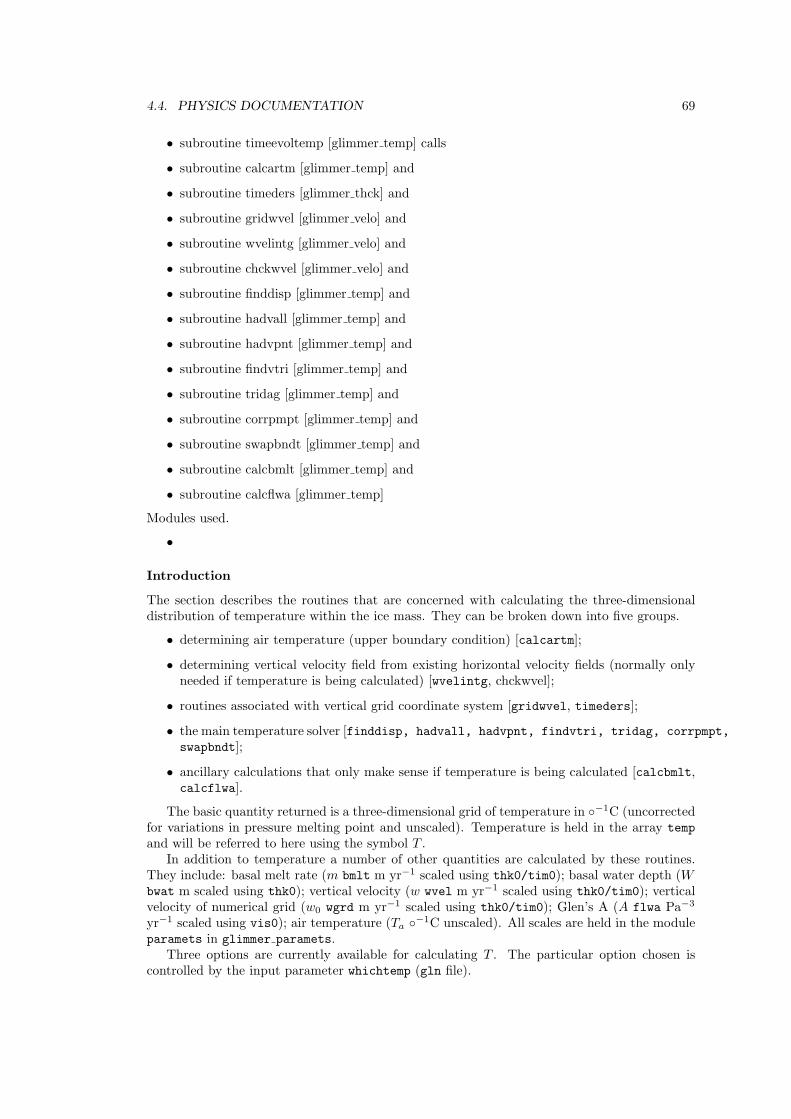
4.4. PHYSICS DOCUMENTATION 69
• subroutine timeevoltemp [glimmer temp] calls
• subroutine calcartm [glimmer temp] and
• subroutine timeders [glimmer thck] and
• subroutine gridwvel [glimmer velo] and
• subroutine wvelintg [glimmer velo] and
• subroutine chckwvel [glimmer velo] and
• subroutine finddisp [glimmer temp] and
• subroutine hadvall [glimmer temp] and
• subroutine hadvpnt [glimmer temp] and
• subroutine findvtri [glimmer temp] and
• subroutine tridag [glimmer temp] and
• subroutine corrpmpt [glimmer temp] and
• subroutine swapbndt [glimmer temp] and
• subroutine calcbmlt [glimmer temp] and
• subroutine calcflwa [glimmer temp]
Modules used.
•
Introduction
The section describes the routines that are concerned with calculating the three-dimensionaldistribution of temperature within the ice mass. They can be broken down into five groups.
• determining air temperature (upper boundary condition) [calcartm];
• determining vertical velocity field from existing horizontal velocity fields (normally onlyneeded if temperature is being calculated) [wvelintg, chckwvel];
• routines associated with vertical grid coordinate system [gridwvel, timeders];
• the main temperature solver [finddisp, hadvall, hadvpnt, findvtri, tridag, corrpmpt,
swapbndt];
• ancillary calculations that only make sense if temperature is being calculated [calcbmlt,calcflwa].
The basic quantity returned is a three-dimensional grid of temperature in ◦−1C (uncorrectedfor variations in pressure melting point and unscaled). Temperature is held in the array temp
and will be referred to here using the symbol T .In addition to temperature a number of other quantities are calculated by these routines.
They include: basal melt rate (m bmlt m yr−1 scaled using thk0/tim0); basal water depth (Wbwat m scaled using thk0); vertical velocity (w wvel m yr−1 scaled using thk0/tim0); verticalvelocity of numerical grid (w0 wgrd m yr−1 scaled using thk0/tim0); Glen’s A (A flwa Pa−3
yr−1 scaled using vis0); air temperature (Ta ◦−1C unscaled). All scales are held in the moduleparamets in glimmer paramets.
Three options are currently available for calculating T . The particular option chosen iscontrolled by the input parameter whichtemp (gln file).
70 CHAPTER 4. DEVELOPER GUIDE
0 Set whole column to the appropriate surface air temperature (Ta).
1 This option is the main solver that determines temperature at the new time step from theappropriate three-dimensional advection-diffusion equation.
2 Set the upper surface temperature to Ta and do a linear interpolation from this value to 0◦C at the lower surface. Check for pressure melting and adjust any temperatures that areabove melting point.
The subroutine timeevoltemp controls calculation of the T etc. It is called in the main timeloop in glimmer object and resides in glimmer temp.
4.5 Configuration File Parser
The run–time behaviour of the ice sheet model is controlled by configuration files. The old fileformat is based on Fortran namelists. The new configuration file format is loosely based onthe format of Windows .ini files with sections containing name/value pairs. The new formatis more flexible and can be easily understood by reading the configuration files. This sectioncontains a description of the configuration file parser API.
4.5.1 File Format
The parser assumes a maximum number of 250 characters per line. Leading and trailing whitespace is ignored. Names are case sensitive.
Comments: Empty lines and lines starting with !, ; or # are ignored.
Sections: Section names are enclosed with square prackets, [] and can be 20 character long.
Parameters: Parameter names are separated from their associated values with either : or =.The names can be 20 characters long. Values can be 200 characters long.
An example configuration file:
;a comment
[a section]
an_int : 1
a_float = 2.0
a_char = hey, this is rather cool
an_array = 10. 20. -10. 40. 100.
[another section]
! more comments
foo : bar
4.5.2 Architecture Overview
The configuration data is stored as linked list. Each section is described by the following listelement:
type ConfigSection
character(len=namelen) :: name
type(ConfigValue), pointer :: values=>NULL()
type(ConfigSection), pointer :: next=>NULL()
end type ConfigSection
4.5. CONFIGURATION FILE PARSER 71
The parameter name/value pairs defined in each section are stored in another linked list:
type ConfigValue
character(len=namelen) :: name
character(len=valuelen) :: value
type(ConfigValue), pointer :: next=>NULL()
end type ConfigValue
These linked lists are setup and read using subroutines.
4.5.3 API
Reading configuration files Configuration files are read using ConfigRead. This subroutineparses the configuration file and populates the linked lists.
subroutine ConfigRead(fname,config)
character(len=*), intent(in) :: fname
type(ConfigSection), pointer :: config
end subroutine ConfigRead
The pointer config contains the first section of the configuration file.
Dumping configuration The subroutine PrintConfig traverses the linked lists and printsthem to standard output.
subroutine PrintConfig(config)
type(ConfigSection), pointer :: config
end subroutine PrintConfig(config)
Searching for a Section The subroutine GetSection can be used to find a specific section.
subroutine GetSection(config,found,name)
type(ConfigSection), pointer :: config
type(ConfigSection), pointer :: found
character(len=*),intent(in) :: name
end subroutine GetSection
On exit the pointer found will point to the first section called name. found points toNULL() if the section name is not found.
Reading parameters Paramter name/value pairs are found using the GetValue family ofsubroutines. GetValue provides an interface to the individual subroutines GetValueChar,GetValueInt, GetValueReal, GetValueIntArray and GetValueRealArray.
subroutine GetValue(section,name,val)
type(ConfigSection), pointer :: section
character(len=*),intent(in) :: name
sometype :: val
integer,intent(in), optional :: numval
end subroutine GetValue
section is the section that should be searched for the parameter name. On exit val
contains the parameter value if it is found, otherwise it is unchanged.
The array versions of GetValue expect value to be a pointer to a one–dimensional array.val is deallocated if it was allocated on entry. The array versions of GetValue also acceptan optional value, numval, with which the maximum number of array elements can be set.The default is 100. Array elements are separated by white space.
72 CHAPTER 4. DEVELOPER GUIDE
4.6 netCDF I/O
The netCDF5 library is used for platform independent, binary file I/O. GLIMMER makes useof the f90 netCDF interface. The majority of the source files are automatically generated fromtemplate files and a variable definition file using a python script. The netCDF files adhere tothe CF6 convention for naming climatic variables. The netCDF files also store parameters usedto define the geographic projection.
The netCDF related functionality is split up so that other subsystems of the model can easilydefine their own variable sets without the need to recompile the main model. These subsystemscan also define their own dimensions and access the dimensions defined by other subsystems.The only restriction is that names should not clash. Have a look at the implementation of theeis climate driver.
4.6.1 Data Structures
Information associated with each dataset is stored in the glimmer nc stat type. Variable anddimension ids are retrived from the data set by using the relevant netCDF library calls. Metadata (such as title, institution and comments) is stored in the derived type glimmer nc meta.
Input and output files are managed by two separate linked lists. Elements of the input filelist contain the number of available time slices and information describing which time slice(s)should be read. Output file elements describe how often data should be written and the currenttime.
4.6.2 The Code Generator
Much of the code needed to do netCDF I/O is very repetative and can therefore be automaticallygenerated. The code generator, generate ncvars.py, is written in python and produces sourcefiles from a template ncdf template.in and the variable definition file, see Section 4.6.3. Thetemplates are valid source files, all the generator does is replace special comments with thecode generated from the variable file. For further information check the documentation ofgenerate ncvars.py7.
4.6.3 Variable Definition File
All netCDF variables are defined in control files, MOD vars.def, where MOD is the name of themodel subsystem. Variables can be modified/added by editing these files. The file is readusing the python ConfigParser module. The format of the file is similar to Windows .ini
files, lines beginning with # or ; or empty lines are ignored. These files must have a definitionsection [VARSET] (see Table 4.1).A new variable definition block starts with the variable namein square brackets []. Variables are further specified by parameter name/value pairs which areseparated by : or =. Parameter names and their meanings are summarised in Table 4.2. Allparameter names not recognised by the code generator (i.e. not in Table 4.2) are added asvariable attributes.
5http://www.unidata.ucar.edu/packages/netcdf/6http://www.cgd.ucar.edu/cms/eaton/cf-metadata/index.html7run pydoc generate ncvars.py
4.6. NETCDF I/O 73
name description
name Name of the model subsystem, e.g. glide. The f90 file is renamedbased on this name. The f90 module and module procedures areprefixed with this name.
datatype The name of the f90 type on which the netCDF variables depend.datamod The name of f90 module in which the f90 type, datatype, is de-
fined.
Table 4.1: Each variable definition file must have a section, called [VARSET], containing theparameters described above.
name description
dimensions List of comma separated dimension names of the variable. Cnotation is used here, i.e. the slowest varying dimension is listedfirst.
data The variable to be stored/loaded. The f90 variable is assumed tohave one dimension smaller than the netCDF variable, i.e. f90variables are always snapshots of the present state of the model.Variables which do not depend on time are not handled automat-ically. Typically, these variables are filled when the netCDF fileis created.
factor Variables are multiplied with this factor on output and divided bythis factor on input. Default: 1.
load Set to 1 if the variable can be loaded from file. Default: 0.hot Set to 1 if the variable should be saved for hot–starting the model
(implies load=1)average Set to 1 if the variable should also be available as a mean over
the write–out interval. Averages are only calculated if they arerequired. To store the average in a netCDF output file appendtavg to the variable.
units UDUNITS compatible unit string describing the variable units.long name A more descriptive name of the variable.standard name The corresponding standard name defined by the CF standard.
Table 4.2: List of accepted variable definition parameters.

74 CHAPTER 4. DEVELOPER GUIDE
Part III
Appendix
75

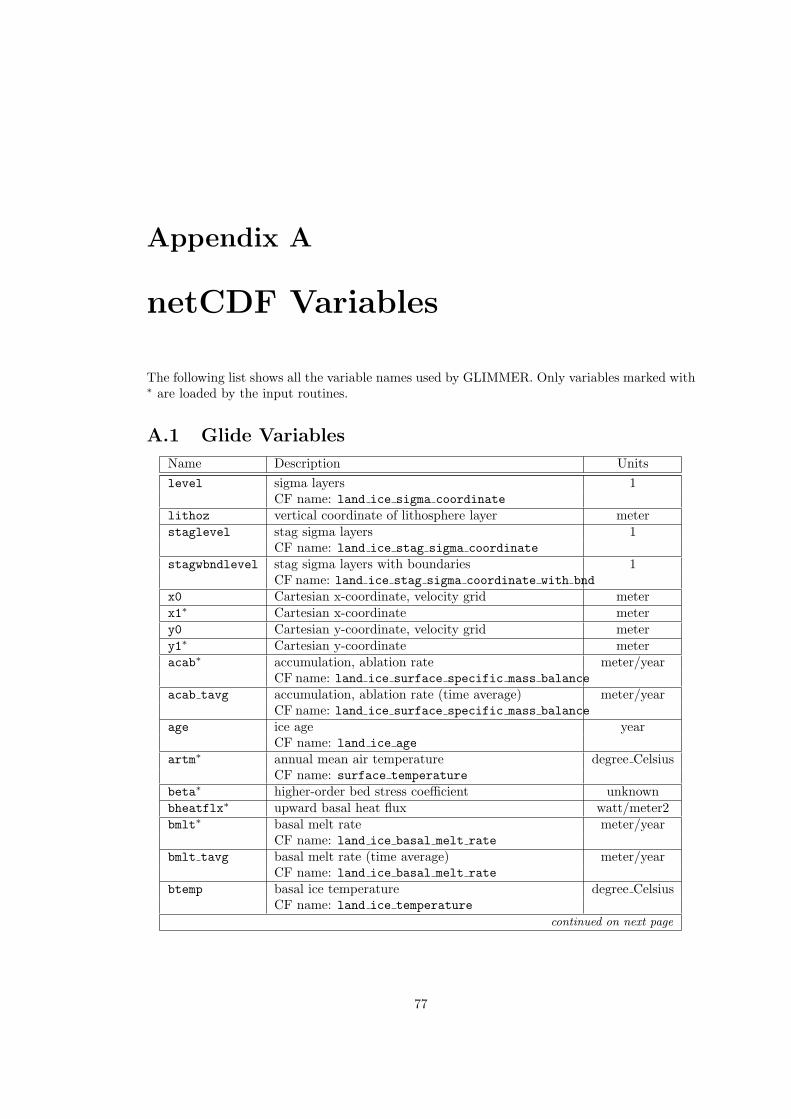
Appendix A
netCDF Variables
The following list shows all the variable names used by GLIMMER. Only variables marked with∗ are loaded by the input routines.
A.1 Glide Variables
Name Description Units
level sigma layers 1CF name: land ice sigma coordinate
lithoz vertical coordinate of lithosphere layer meterstaglevel stag sigma layers 1
CF name: land ice stag sigma coordinate
stagwbndlevel stag sigma layers with boundaries 1CF name: land ice stag sigma coordinate with bnd
x0 Cartesian x-coordinate, velocity grid meterx1∗ Cartesian x-coordinate metery0 Cartesian y-coordinate, velocity grid metery1∗ Cartesian y-coordinate meteracab∗ accumulation, ablation rate meter/year
CF name: land ice surface specific mass balance
acab tavg accumulation, ablation rate (time average) meter/yearCF name: land ice surface specific mass balance
age ice age yearCF name: land ice age
artm∗ annual mean air temperature degree CelsiusCF name: surface temperature
beta∗ higher-order bed stress coefficient unknownbheatflx∗ upward basal heat flux watt/meter2bmlt∗ basal melt rate meter/year
CF name: land ice basal melt rate
bmlt tavg basal melt rate (time average) meter/yearCF name: land ice basal melt rate
btemp basal ice temperature degree CelsiusCF name: land ice temperature
continued on next page
77
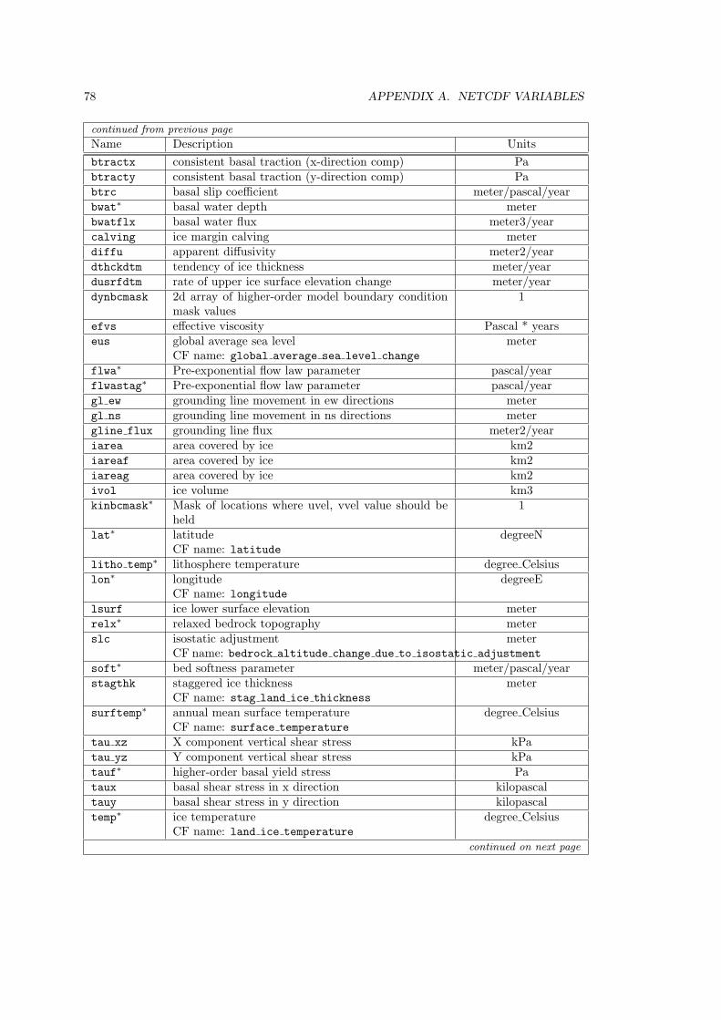
78 APPENDIX A. NETCDF VARIABLES
continued from previous page
Name Description Units
btractx consistent basal traction (x-direction comp) Pabtracty consistent basal traction (y-direction comp) Pabtrc basal slip coefficient meter/pascal/yearbwat∗ basal water depth meterbwatflx basal water flux meter3/yearcalving ice margin calving meterdiffu apparent diffusivity meter2/yeardthckdtm tendency of ice thickness meter/yeardusrfdtm rate of upper ice surface elevation change meter/yeardynbcmask 2d array of higher-order model boundary condition
mask values1
efvs effective viscosity Pascal * yearseus global average sea level meter
CF name: global average sea level change
flwa∗ Pre-exponential flow law parameter pascal/yearflwastag∗ Pre-exponential flow law parameter pascal/yeargl ew grounding line movement in ew directions metergl ns grounding line movement in ns directions metergline flux grounding line flux meter2/yeariarea area covered by ice km2iareaf area covered by ice km2iareag area covered by ice km2ivol ice volume km3kinbcmask∗ Mask of locations where uvel, vvel value should be
held1
lat∗ latitude degreeNCF name: latitude
litho temp∗ lithosphere temperature degree Celsiuslon∗ longitude degreeE
CF name: longitudelsurf ice lower surface elevation meterrelx∗ relaxed bedrock topography meterslc isostatic adjustment meter
CF name: bedrock altitude change due to isostatic adjustment
soft∗ bed softness parameter meter/pascal/yearstagthk staggered ice thickness meter
CF name: stag land ice thickness
surftemp∗ annual mean surface temperature degree CelsiusCF name: surface temperature
tau xz X component vertical shear stress kPatau yz Y component vertical shear stress kPatauf∗ higher-order basal yield stress Pataux basal shear stress in x direction kilopascaltauy basal shear stress in y direction kilopascaltemp∗ ice temperature degree Celsius
CF name: land ice temperature
continued on next page
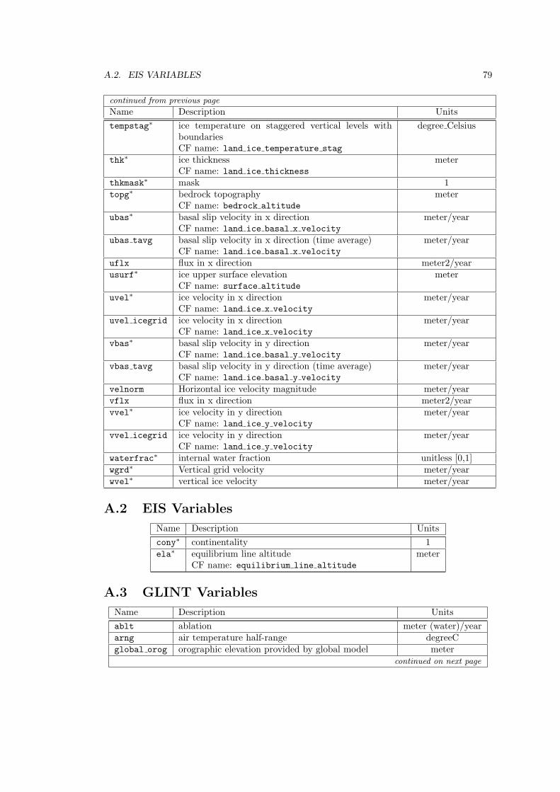
A.2. EIS VARIABLES 79
continued from previous page
Name Description Units
tempstag∗ ice temperature on staggered vertical levels withboundaries
degree Celsius
CF name: land ice temperature stag
thk∗ ice thickness meterCF name: land ice thickness
thkmask∗ mask 1topg∗ bedrock topography meter
CF name: bedrock altitude
ubas∗ basal slip velocity in x direction meter/yearCF name: land ice basal x velocity
ubas tavg basal slip velocity in x direction (time average) meter/yearCF name: land ice basal x velocity
uflx flux in x direction meter2/yearusurf∗ ice upper surface elevation meter
CF name: surface altitude
uvel∗ ice velocity in x direction meter/yearCF name: land ice x velocity
uvel icegrid ice velocity in x direction meter/yearCF name: land ice x velocity
vbas∗ basal slip velocity in y direction meter/yearCF name: land ice basal y velocity
vbas tavg basal slip velocity in y direction (time average) meter/yearCF name: land ice basal y velocity
velnorm Horizontal ice velocity magnitude meter/yearvflx flux in x direction meter2/yearvvel∗ ice velocity in y direction meter/year
CF name: land ice y velocity
vvel icegrid ice velocity in y direction meter/yearCF name: land ice y velocity
waterfrac∗ internal water fraction unitless [0,1]wgrd∗ Vertical grid velocity meter/yearwvel∗ vertical ice velocity meter/year
A.2 EIS Variables
Name Description Units
cony∗ continentality 1ela∗ equilibrium line altitude meter
CF name: equilibrium line altitude
A.3 GLINT Variables
Name Description Units
ablt ablation meter (water)/yeararng air temperature half-range degreeCglobal orog orographic elevation provided by global model meter
continued on next page
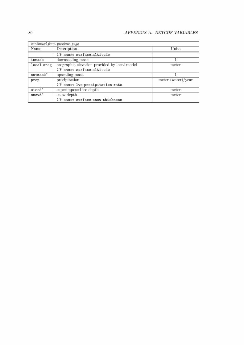
80 APPENDIX A. NETCDF VARIABLES
continued from previous page
Name Description Units
CF name: surface altitude
inmask downscaling mask 1local orog orographic elevation provided by local model meter
CF name: surface altitude
outmask∗ upscaling mask 1prcp precipitation meter (water)/year
CF name: lwe precipitation rate
siced∗ superimposed ice depth metersnowd∗ snow depth meter
CF name: surface snow thickness
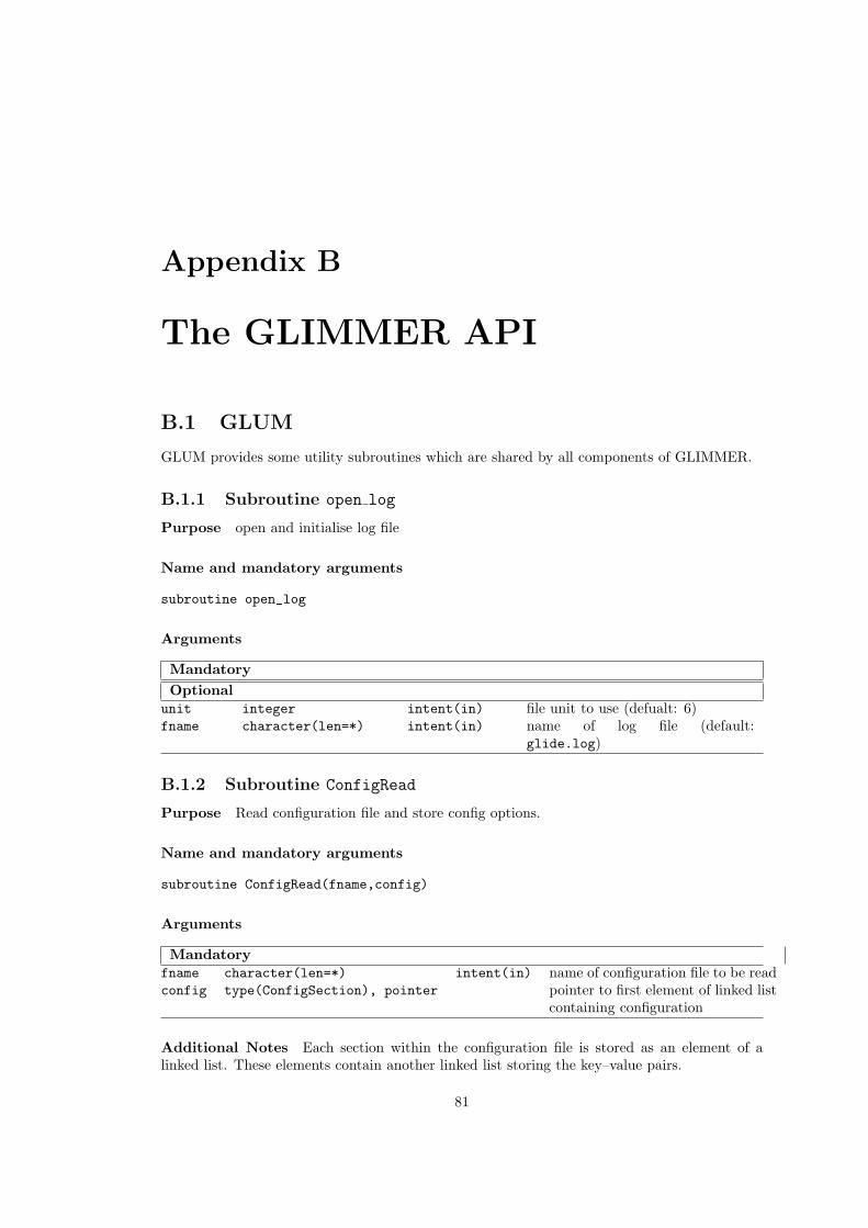
Appendix B
The GLIMMER API
B.1 GLUM
GLUM provides some utility subroutines which are shared by all components of GLIMMER.
B.1.1 Subroutine open log
Purpose open and initialise log file
Name and mandatory arguments
subroutine open_log
Arguments
Mandatory
Optionalunit integer intent(in) file unit to use (defualt: 6)fname character(len=*) intent(in) name of log file (default:
glide.log)
B.1.2 Subroutine ConfigRead
Purpose Read configuration file and store config options.
Name and mandatory arguments
subroutine ConfigRead(fname,config)
Arguments
Mandatoryfname character(len=*) intent(in) name of configuration file to be readconfig type(ConfigSection), pointer pointer to first element of linked list
containing configuration
Additional Notes Each section within the configuration file is stored as an element of alinked list. These elements contain another linked list storing the key–value pairs.
81
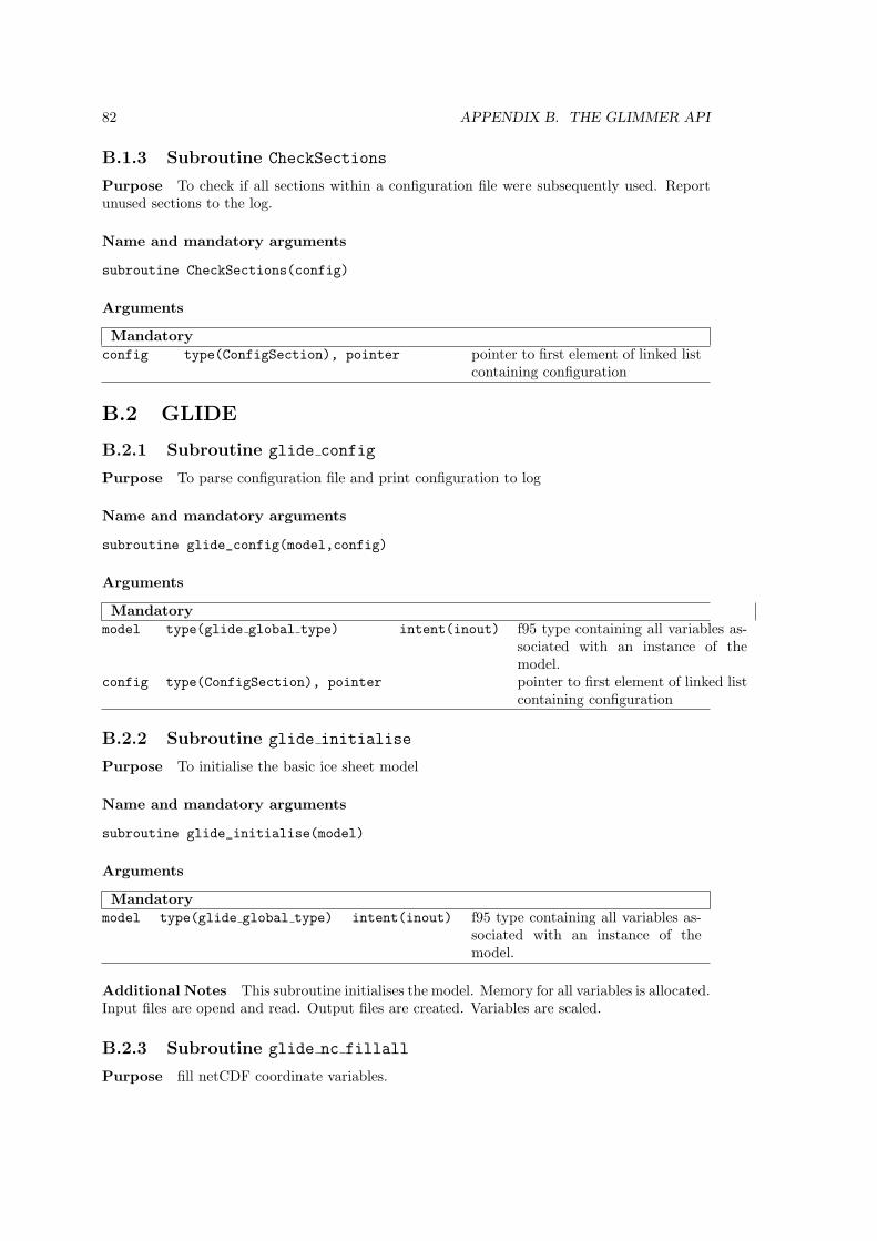
82 APPENDIX B. THE GLIMMER API
B.1.3 Subroutine CheckSections
Purpose To check if all sections within a configuration file were subsequently used. Reportunused sections to the log.
Name and mandatory arguments
subroutine CheckSections(config)
Arguments
Mandatoryconfig type(ConfigSection), pointer pointer to first element of linked list
containing configuration
B.2 GLIDE
B.2.1 Subroutine glide config
Purpose To parse configuration file and print configuration to log
Name and mandatory arguments
subroutine glide_config(model,config)
Arguments
Mandatorymodel type(glide global type) intent(inout) f95 type containing all variables as-
sociated with an instance of themodel.
config type(ConfigSection), pointer pointer to first element of linked listcontaining configuration
B.2.2 Subroutine glide initialise
Purpose To initialise the basic ice sheet model
Name and mandatory arguments
subroutine glide_initialise(model)
Arguments
Mandatorymodel type(glide global type) intent(inout) f95 type containing all variables as-
sociated with an instance of themodel.
Additional Notes This subroutine initialises the model. Memory for all variables is allocated.Input files are opend and read. Output files are created. Variables are scaled.
B.2.3 Subroutine glide nc fillall
Purpose fill netCDF coordinate variables.
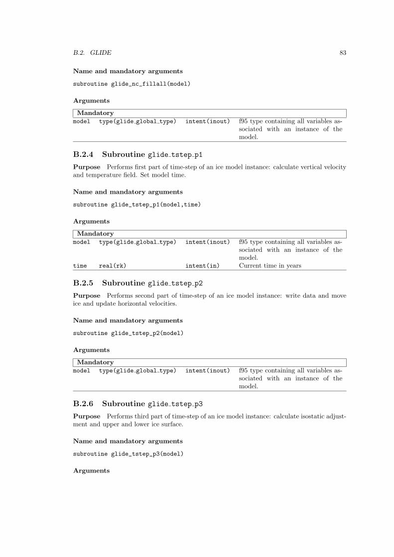
B.2. GLIDE 83
Name and mandatory arguments
subroutine glide_nc_fillall(model)
Arguments
Mandatorymodel type(glide global type) intent(inout) f95 type containing all variables as-
sociated with an instance of themodel.
B.2.4 Subroutine glide tstep p1
Purpose Performs first part of time-step of an ice model instance: calculate vertical velocityand temperature field. Set model time.
Name and mandatory arguments
subroutine glide_tstep_p1(model,time)
Arguments
Mandatorymodel type(glide global type) intent(inout) f95 type containing all variables as-
sociated with an instance of themodel.
time real(rk) intent(in) Current time in years
B.2.5 Subroutine glide tstep p2
Purpose Performs second part of time-step of an ice model instance: write data and moveice and update horizontal velocities.
Name and mandatory arguments
subroutine glide_tstep_p2(model)
Arguments
Mandatorymodel type(glide global type) intent(inout) f95 type containing all variables as-
sociated with an instance of themodel.
B.2.6 Subroutine glide tstep p3
Purpose Performs third part of time-step of an ice model instance: calculate isostatic adjust-ment and upper and lower ice surface.
Name and mandatory arguments
subroutine glide_tstep_p3(model)
Arguments
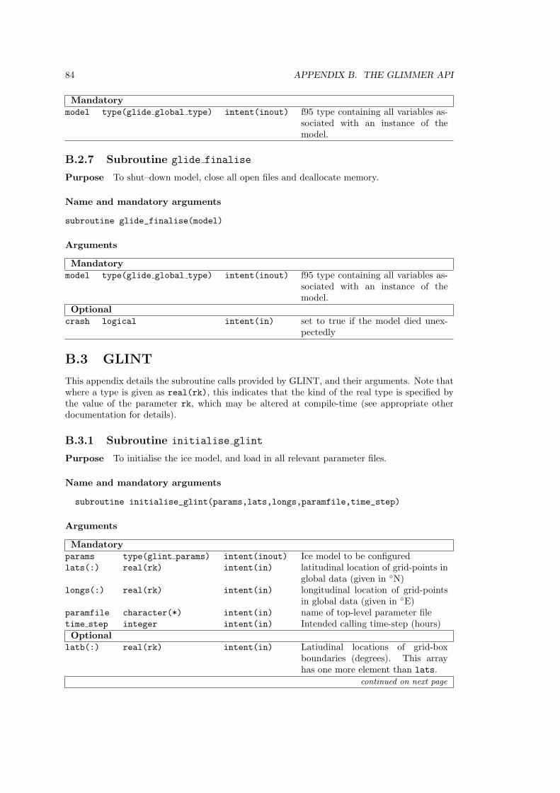
84 APPENDIX B. THE GLIMMER API
Mandatorymodel type(glide global type) intent(inout) f95 type containing all variables as-
sociated with an instance of themodel.
B.2.7 Subroutine glide finalise
Purpose To shut–down model, close all open files and deallocate memory.
Name and mandatory arguments
subroutine glide_finalise(model)
Arguments
Mandatorymodel type(glide global type) intent(inout) f95 type containing all variables as-
sociated with an instance of themodel.
Optionalcrash logical intent(in) set to true if the model died unex-
pectedly
B.3 GLINT
This appendix details the subroutine calls provided by GLINT, and their arguments. Note thatwhere a type is given as real(rk), this indicates that the kind of the real type is specified bythe value of the parameter rk, which may be altered at compile-time (see appropriate otherdocumentation for details).
B.3.1 Subroutine initialise glint
Purpose To initialise the ice model, and load in all relevant parameter files.
Name and mandatory arguments
subroutine initialise_glint(params,lats,longs,paramfile,time_step)
Arguments
Mandatoryparams type(glint params) intent(inout) Ice model to be configuredlats(:) real(rk) intent(in) latitudinal location of grid-points in
global data (given in ◦N)longs(:) real(rk) intent(in) longitudinal location of grid-points
in global data (given in ◦E)paramfile character(*) intent(in) name of top-level parameter filetime step integer intent(in) Intended calling time-step (hours)Optional
latb(:) real(rk) intent(in) Latiudinal locations of grid-boxboundaries (degrees). This arrayhas one more element than lats.
continued on next page
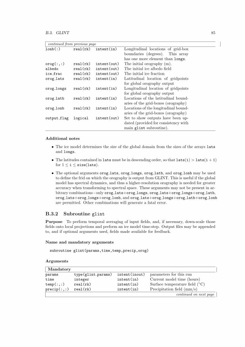
B.3. GLINT 85
continued from previous page
lonb(:) real(rk) intent(in) Longitudinal locations of grid-boxboundaries (degrees). This arrayhas one more element than longs.
orog(:,:) real(rk) intent(out) The initial orography (m).albedo real(rk) intent(out) The initial ice albedo fieldice frac real(rk) intent(out) The initial ice fractionorog lats real(rk) intent(in) Latitudinal location of gridpoints
for global orography outputorog longs real(rk) intent(in) Longitudinal location of gridpoints
for global orography outputorog latb real(rk) intent(in) Locations of the latitudinal bound-
aries of the grid-boxes (orography)orog lonb real(rk) intent(in) Locations of the longitudinal bound-
aries of the grid-boxes (orography)output flag logical intent(out) Set to show outputs have been up-
dated (provided for consistency withmain glint subroutine).
Additional notes
• The ice model determines the size of the global domain from the sizes of the arrays latsand longs.
• The latitudes contained in latsmust be in descending order, so that lats(i) > lats(i+ 1)for 1 ≤ i ≤ size(lats).
• The optional arguments orog lats, orog longs, orog latb, and orog lonb may be usedto define the frid on which the orography is output from GLINT. This is useful if the globalmodel has spectral dynamics, and thus a higher-resolution orography is needed for greateraccuracy when transforming to spectral space. These arguments may not be present in ar-bitrary combinations - only orog lats+orog longs, orog lats+orog longs+orog latb,orog lats+orog longs+orog lonb, and orog lats+orog longs+orog latb+orog lonb
are permitted. Other combinations will generate a fatal error.
B.3.2 Subroutine glint
Purpose To perform temporal averaging of input fields, and, if necessary, down-scale thosefields onto local projections and perform an ice model time-step. Output files may be appendedto, and if optional arguments used, fields made available for feedback.
Name and mandatory arguments
subroutine glint(params,time,temp,precip,orog)
Arguments
Mandatoryparams type(glint params) intent(inout) parameters for this runtime integer intent(in) Current model time (hours)temp(:,:) real(rk) intent(in) Surface temperature field (◦C)precip(:,:) real(rk) intent(in) Precipitation field (mm/s)
continued on next page
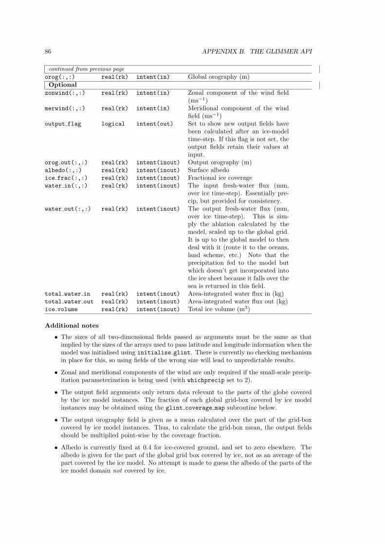
86 APPENDIX B. THE GLIMMER API
continued from previous page
orog(:,:) real(rk) intent(in) Global orography (m)Optional
zonwind(:,:) real(rk) intent(in) Zonal component of the wind field(ms−1)
merwind(:,:) real(rk) intent(in) Meridional component of the windfield (ms−1)
output flag logical intent(out) Set to show new output fields havebeen calculated after an ice-modeltime-step. If this flag is not set, theoutput fields retain their values atinput.
orog out(:,:) real(rk) intent(inout) Output orography (m)albedo(:,:) real(rk) intent(inout) Surface albedoice frac(:,:) real(rk) intent(inout) Fractional ice coveragewater in(:,:) real(rk) intent(inout) The input fresh-water flux (mm,
over ice time-step). Essentially pre-cip, but provided for consistency.
water out(:,:) real(rk) intent(inout) The output fresh-water flux (mm,over ice time-step). This is sim-ply the ablation calculated by themodel, scaled up to the global grid.It is up to the global model to thendeal with it (route it to the oceans,land scheme, etc.) Note that theprecipitation fed to the model butwhich doesn’t get incorporated intothe ice sheet because it falls over thesea is returned in this field.
total water in real(rk) intent(inout) Area-integrated water flux in (kg)total water out real(rk) intent(inout) Area-integrated water flux out (kg)ice volume real(rk) intent(inout) Total ice volume (m3)
Additional notes
• The sizes of all two-dimensional fields passed as arguments must be the same as thatimplied by the sizes of the arrays used to pass latitude and longitude information when themodel was initialised using initialise glint. There is currently no checking mechanismin place for this, so using fields of the wrong size will lead to unpredictable results.
• Zonal and meridional components of the wind are only required if the small-scale precip-itation parameterization is being used (with whichprecip set to 2).
• The output field arguments only return data relevant to the parts of the globe coveredby the ice model instances. The fraction of each global grid-box covered by ice modelinstances may be obtained using the glint coverage map subroutine below.
• The output orography field is given as a mean calculated over the part of the grid-boxcovered by ice model instances. Thus, to calculate the grid-box mean, the output fieldsshould be multiplied point-wise by the coverage fraction.
• Albedo is currently fixed at 0.4 for ice-covered ground, and set to zero elsewhere. Thealbedo is given for the part of the global grid box covered by ice, not as an average of thepart covered by the ice model. No attempt is made to guess the albedo of the parts of theice model domain not covered by ice.
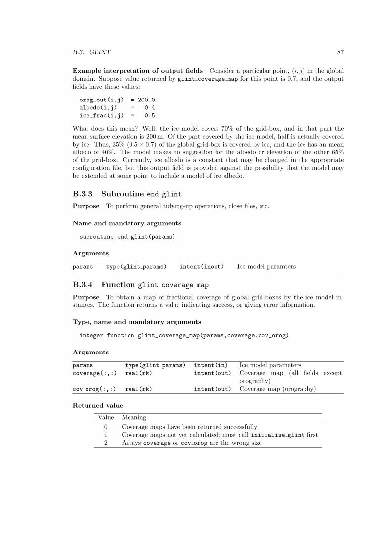
B.3. GLINT 87
Example interpretation of output fields Consider a particular point, (i, j) in the globaldomain. Suppose value returned by glint coverage map for this point is 0.7, and the outputfields have these values:
orog_out(i,j) = 200.0
albedo(i,j) = 0.4
ice_frac(i,j) = 0.5
What does this mean? Well, the ice model covers 70% of the grid-box, and in that part themean surface elevation is 200m. Of the part covered by the ice model, half is actually coveredby ice. Thus, 35% (0.5× 0.7) of the global grid-box is covered by ice, and the ice has an meanalbedo of 40%. The model makes no suggestion for the albedo or elevation of the other 65%of the grid-box. Currently, ice albedo is a constant that may be changed in the appropriateconfiguration file, but this output field is provided against the possibility that the model maybe extended at some point to include a model of ice albedo.
B.3.3 Subroutine end glint
Purpose To perform general tidying-up operations, close files, etc.
Name and mandatory arguments
subroutine end_glint(params)
Arguments
params type(glint params) intent(inout) Ice model paramters
B.3.4 Function glint coverage map
Purpose To obtain a map of fractional coverage of global grid-boxes by the ice model in-stances. The function returns a value indicating success, or giving error information.
Type, name and mandatory arguments
integer function glint_coverage_map(params,coverage,cov_orog)
Arguments
params type(glint params) intent(in) Ice model parameterscoverage(:,:) real(rk) intent(out) Coverage map (all fields except
orography)cov orog(:,:) real(rk) intent(out) Coverage map (orography)
Returned value
Value Meaning
0 Coverage maps have been returned successfully1 Coverage maps not yet calculated; must call initialise glint first2 Arrays coverage or cov orog are the wrong size