Faculty of Mathematics

and Natural Sciences

Giving a step-by-step reduction

from SAT to TSP and giving

some remarks on Neil

Tennant's Changes of Mind

Bachelor Thesis Mathematics

July 2014

Student: M.M. Bronts

Supervisors: Prof. dr. J. Top and Prof. dr. B.P. Kooi

Abstract

Karp wrote an article about 21 decision problems. He gave instances for poly-nomial reductions between these problems, but he did not prove that theseinstances actually worked. In this thesis we will first prove that some of theseinstances are indeed correct. Second we will give some remarks on a beliefcontraction problem given by Neil Tennant in his book Changes of Mind. Hedescribes what happens in our mind when we change our mind and argues thatthis is an NP-complete decision problem.

2

Contents

1 Introduction 4

2 Historical background 5

3 Introductory definitions and decision problems 73.1 The Turing machine . . . . . . . . . . . . . . . . . . . . . . . . . . . . 73.2 Some important definitions . . . . . . . . . . . . . . . . . . . . . . . . 73.3 Decision problems . . . . . . . . . . . . . . . . . . . . . . . . . . . . . 8

4 The Boolean satisfiability problem 104.1 Propositional logic . . . . . . . . . . . . . . . . . . . . . . . . . . . . . 104.2 Polynomial functions over F2 . . . . . . . . . . . . . . . . . . . . . . . 114.3 SAT . . . . . . . . . . . . . . . . . . . . . . . . . . . . . . . . . . . . . 13

5 Complexity theory and reduction 155.1 Complexity theory . . . . . . . . . . . . . . . . . . . . . . . . . . . . . 155.2 Polynomial time reduction . . . . . . . . . . . . . . . . . . . . . . . . . 175.3 Example: 3-SAT is NP-complete . . . . . . . . . . . . . . . . . . . . . 19

6 Reduction of SAT to TSP 236.1 SAT � CLIQUE . . . . . . . . . . . . . . . . . . . . . . . . . . . . . . 236.2 CLIQUE � VC . . . . . . . . . . . . . . . . . . . . . . . . . . . . . . . 246.3 VC � HC . . . . . . . . . . . . . . . . . . . . . . . . . . . . . . . . . . 256.4 HC � TSP . . . . . . . . . . . . . . . . . . . . . . . . . . . . . . . . . 29

7 Remarks on Changes of Mind by Neil Tennant 317.1 Tennant’s belief system . . . . . . . . . . . . . . . . . . . . . . . . . . 317.2 The contraction problem . . . . . . . . . . . . . . . . . . . . . . . . . . 347.3 How realistic is Tennant’s belief system? . . . . . . . . . . . . . . . . . 357.4 Can you say something about the complexity of a problem about the

mind? . . . . . . . . . . . . . . . . . . . . . . . . . . . . . . . . . . . . 36

8 Conclusion 39

3

1 Introduction

This thesis is about problems that can be answered with ‘yes’ or ‘no’, so-called decisionproblems. We focus especially on the Boolean satisfiability problem (SAT). This is aproblem that has to do with propositional logic. You are given a propositional formulaand the question is whether there is a satisfying truth assignment. That is, whetheryou can give an assignment of truth values to the variables in the propositional formulathat makes the formula true. If there is such an assignment, the answer to the decisionproblem is ‘yes’. For example, (p ∨ ¬q) → (p ∧ q) is satisfiable, since making bothp and q true makes the formula true. The Boolean satisfiability problem is the firstproblem that was shown to be NP-complete. NP-complete is, next to P and NP, animportant complexity class in complexity theory. When a problem is NP-complete,the problem is in the complexity class NP and every other problem which is in theclass NP can be reduced quickly (in polynomial time) to it. Informally, the class Pcontains all decision problems that can be solved in polynomial time and the class NPcontains all decision problems of which it can be verified in polynomial time whetherthere is a solution.

In the first part of this thesis the focus lies on polynomial time reductions used toshow that a problem is NP-complete. A given decision problem in the class NP canbe shown to be NP-complete by reducing another problem, of which we already knowit to be NP-complete, to it. This process of reducing problems produces a scheme ofreductions. The Boolean satisfiability problem is at the center of this scheme and wewill show that the problem can be reduced step by step in polynomial time to theTraveling Salesman Problem (TSP), another problem in this scheme, see Figure 3.TSP is about a man who has to visit a certain number of cities. It costs money todrive from one city to another and the salesman has to find the cheapest way to visiteach city exactly once. The decision version is then to find out whether such a tourexists without exceeding a given amount of money. TSP is not directly connectedto SAT in this scheme, there are some reductions in between. In this thesis we willlook at the reduction process from SAT to TSP. We know that both problems areNP-complete, so in theory there exists a direct reduction. Finding a direct reductionproved to be difficult, so we will reduce SAT to TSP via CLIQUE, Vertex Coverand Hamiltonian Circuit. In an article by Karp [1972, p. 97-98] instances of thesereductions are given but Karp did not provide detailed proofs. Some of these proveswill be given in this thesis.

We will start with some historical background on the mathematics which led tothe development of complexity theory. We will mention George Boole, the founderof Boolean Algebra, Kurt Godel, who questioned the provability of statements, AlanTuring, the inventor of the Turing machine and Stephen Arthur Cook, a mathemati-cian who is specialized in computational complexity theory. In Section 3 we explainbriefly how a Turing machine works and give some important definitions which weneed to understand the decision problems that are mentioned. The fourth sectionstarts with a short introduction to propositional logic and an introduction to polyno-mial functions over F2 before stating the problem SAT. In Section 5 complexity theorywill be explained and definitions of the three most important complexity classes asmentioned above are given. We will also define what a reduction is and give as exam-ple the reduction from SAT to 3-SAT. In Section 6 we will reduce SAT to TSP viaCLIQUE, Vertex Cover and Hamiltonian Circuit. In the last section we will use theknowledge about complexity to say something about the book Changes of mind byNeil Tennant. Tennant describes a contraction problem, which is about changing be-liefs. It is a decision problem, and Tennant proves that his problem is NP-complete.We discuss whether the system of beliefs, as represented by Tennant, is a realisticrepresentation of the mind and we discuss whether we can say something about thecomplexity of a problem about the mind.

4

2 Historical background

In the middle of the nineteenth century mathematics became more abstract. Math-ematicians started thinking that mathematics was more than just calculation tech-niques. They discovered that mathematics was based on formal structures, axiomsand philosophical ideas. George Boole (1815-1864) and Augustus De Morgan (1806-1871), two British logicians, came up with important systems for deductive reasoning,which formally captures the idea that a conclusion follows logically from some set ofpremises. Boole is known for his book An Investigation of the Laws of Thought inwhich he, as the title suggests, wants

[...] to investigate the fundamental laws of those operations of the mind bywhich reasoning is performed; to give expression to them in the symbolicallanguage of a Calculus, and upon this foundation to establish the scienceof Logic and construct its method; [...] [Boole, 1854, p. 1]

Boole also discovered Boolean Algebra in which he reduces logic to algebra. Hethought of mathematical propositions as being true or not true, 1 or 0 respectively.This will be of importance in the Boolean satisfiability problem, a decision problemwhich plays a central role in this thesis and will be treated in Section 4.

In the beginning of the twentieth century formalism was upcoming. Formalismsays that mathematics is completely built up of (strings of) symbols which are ma-nipulated by formal rules. Starting with a string of symbols to which we can applythe formal rules, we generate new strings (see the tq-system in ??). The influentialmathematician David Hilbert (1862-1943) made it possible to develop the formalistschool. He believed that logic was the foundation of mathematics. Hilbert thoughtthat for every true statement in mathematics there could be found a proof (complete-ness) and that it could be proven that there was no contradiction in the formal system(consistency). Kurt Godel (1906-1978) criticized the completeness of formal systemsand proved his Incompleteness Theorems. These theorems mark a crucial point inthe history of mathematics. It was because of these theorems that mathematiciansbecame interested in the question what can be proved and what cannot. Hofstadter(1945-) wrote the book Godel, Escher, Bach: An eternal golden braid in which hecombines mathematics with art and music in a philosophical way. He popularizes thework of Godel, Escher and Bach and has no direct influence on mathematical research.In this book he mentions one of the Incompleteness theorems of Godel briefly, butconcludes that it is too hard to understand it immediately: “The Theorem can belikened to a pearl, and the method of proof to an oyster. The pearl is prized for itsluster and simplicity; the oyster is a complex living beast whose innards give rise tothis mysteriously simple gem” [Hofstadter, 1979, p. 17]. Hofstadter therefore gives “aparaphrase in more normal English: All consistent axiomatic formulations of numbertheory include undecidable propositions” [Hofstadter, 1979, p. 17]. Although we willnot elaborate on the theorems themselves, these theorems gave rise to the centralquestions in complexity theory: ‘Where lies the boundary between computable andnot computable?’ and ‘When is a computational problem easy or hard to solve?’

Around 1936 mathematicians became more and more interested in questions aboutcomplexity. Because of this, it was necessary to know how a computational processworks. Alan Turing (1912-1954) therefore, stated exactly what a computation is. Heinvented the Turing machine in 1937, which is an abstract machine that can imitateany formal system. In the next section we will explain briefly how this machine works.The invention of the Turing machine was one of the most important inventions forfurther research in complexity theory. The machine was used to show whether some-thing was computable and it could also tell how long it took for a certain algorithm tofind an answer. The invention of the Turing machine was important because peoplecould now look at the behavior of these algorithms to find out whether they are easyor hard to solve. This was done by looking at the time and space (memory) the Turingmachine, and later the computer, needed to solve the problem or to conclude that

5

there was no solution. These problems were placed in different complexity classesaccording to their computational difficulty. Later on in this thesis we will introducethe most important classes: P, NP and NP-complete.

Stephen Arthur Cook (1939-) is an American mathematician who is specialized incomputational complexity theory. In 1971 he wrote a paper in which he introducedsome new terms to study this subject. He also came up with a proof that there isat least one NP-complete problem, namely the Boolean satisfiability problem (SAT).Independently of him, Leonid Levin (1948-) came up with a proof of the same theorem.SAT was the first decision problem which was proven to be NP-complete. In short,this means that any problem in NP to which SAT could be reduced, would also be NP-complete. In 1971 Cook stated one of the Millennium Prize Problems1, namely the‘P versus NP’ problem. It is a problem about computationality which asks whether itis true that P = NP . In the introduction we mentioned briefly what the complexityclasses P and NP are. Namely, the class P contains all decision problems that can besolved in polynomial time and the class NP contains all decision problems of whichit can be verified in polynomial time whether there is a solution. When a problemis NP-complete, the problem is in the complexity class NP and every other problemwhich is in the class NP can be reduced quickly (in polynomial time) to it. From thisinformal definition of NP-completeness it follows that if we can show that a problemin NP-complete can be solved in polynomial time (or, is in P), then every NP problemcan be solved in polynomial time too. If someone is able to show this, it must be truethat P = NP . Up until now, this problem has still remained unsolved. In Section5.2 we will explain this Millennium Prize Problem briefly after we have given thedefinitions of the complexity classes P, NP and NP-complete.

1Millennium Prize Problems are a couple of problems in mathematics which are very hard tosolve. Therefore, the person who comes up with a correct solution of one of these problems willreceive one million dollars being awarded by the Clay Mathematics Institute. This institute statedseven problems and until now only one has been solved.

6

3 Introductory definitions and decision problems

Decision problems play a central role in this thesis. They are a group of problemsor questions which can be answered with ’yes’ or ’no’. For example, the Booleansatisfiability problem and the Traveling Salesman Problem are decision problems.TSP will be introduced here and we will also briefly explain the Hamiltonian Circuitproblem, the Vertex Cover Problem and the problem CLIQUE. They will be usefulfor finding a good reduction in Section 6. The decision problem SAT needs a bitmore explanation and will therefore be treated in the next section. We will start thissection by introducing Alan Turing’s invention, the Turing machine. After this wewill introduce some important definitions that will be used often in the rest of thisthesis.

3.1 The Turing machine

We want to find out whether problems can be solved within reasonable time or whetherit can be verified that there is a solution. This can be done by a Turing machine.In this thesis we will only explain informally what a Turing machine is. A formaldefinition can be found in [Papadimitriou, 1994, p. 19]. A Turing machine is anabstract automatic machine. A problem can be written as an algorithm and will beimplemented in a Turing machine to find out whether it has a solution. It is a modelof computation which forms a basic structure for every computer.

You can think of a Turing machine as a machine that can read and write on aninfinitely long tape with a finite alphabet and a finite set of states, starting in aninitial state. The alphabet often consists of elements from the set {0, 1, B,B}, whereB is the blank symbol and B is the first symbol. There are rules, called transitionfunctions, which tell the machine what has to be done in which state. Some examplesof these functions are: replacing the symbol by another one, move left or right, changethe current state or stop and give output ‘yes’ or ‘no’. When a finite input is given onthe tape, the machine reads the first symbol in the current state. The new symbol themachine reads together with the state the machine is in, determine which transitionfunction will be applied.

As an example we will explain what happens if we want to add two numbers witha Turing machine. Let 11 + 111 be our finite input on the tape, where 11 = 2 and111 = 3. We want to add these numbers such that we get 11111 = 5. Note thata Turing machine does not interpret the symbol +, it is just to separate the twonumbers. The Turing machine starts at the first 1 and goes to the right until hereaches the +. He replaces the + by a 1 and goes to the right. The machine continuesmoving to the right until he reaches a blank symbol B which means that he reachedthe end of the string. We now have the string 111111 which equals 6. The machinegoes one place to the left and replaces the last 1 by a B. The machine then goes backto the start and is finished. He has reached 11111 = 5.

3.2 Some important definitions

To understand decision problems like TSP, Hamiltonian Circuit, Vertex Cover andCLIQUE we will give some important definitions that we will use often in this thesis.For example, we need to know what a (complete) graph and how a graph can berepresented as an adjacency matrix.

Definition 1 (Decision problem). A decision problem is a problem or question thatcan be answered with ‘yes’ or ‘no’.

Graphs are crucial for this thesis, so it helps to understand what a graph is. Forexample, they are used in all the decision problems mentioned above.

2http://www.cis.upenn.edu/~dietzd/CIT596/turingMachine.gif

7

Figure 1: A Turing machine2

Definition 2 (Graph). A graph G is an ordered pair G = (V,E) where V = {1, ..., n}is a set of nodes and E = {(u, v) | u, v ∈ V } is a set of edges.

Definition 3 (Complete graph). A complete graph is a graph G = (V,E) where forevery two nodes u, v ∈ V with u 6= v, we have (u, v) ∈ E.

We can also represent a graph as a binary n × n matrix A. Thus all elements inA are either 0 or 1. We call such a matrix an adjacency matrix.

Definition 4 (Adjacency matrix). Given a graph G, the adjacency matrix A = (Aij)of G is the n× n matrix defined by

Aij =

{0, (i, j) /∈ E1, (i, j) ∈ E

.

We only work with undirected graphs, which means that we have a symmetric matrix,that is, Aij = Aji. We therefore only need to look at the upper half of the matrix.We set Aii = 0, because we do not allow edges that go from a node to itself. Thisrepresentation of a graph we will use later for the understanding of the complexity ofreductions.

3.3 Decision problems

We will now give some examples of decision problems. A well-known decision problemis the Traveling Salesman Problem. Informally is it about a traveling salesman whohas to visit a number of cities. It costs money to drive from one city to another andthe salesman has to find the cheapest way to visit each city exactly once. The decisionversion of TSP is then to find out whether such a tour exists without exceeding a givenamount of money.

Formally we are looking at n cities 1, ..., n, that represent the nodes of a completegraph G. The costs to travel from city vi to vj are denoted by c(vi, vj) ∈ N. Thesecosts are weights attached to the edges of G. Assume that for all i and j c(vi, vj) =c(vj , vi), that is, it takes the same amount of money to travel from city vi to vj asfrom city vj to vi. We now want to find the cheapest tour to visit all the cities exactlyonce. Thus, find a rearrangement π of the the cities 1, ..., n such that(

n−1∑i=1

c(vπ(i), vπ(i+1))

)+ c(vπ(n), vπ(1)) (1)

is minimized. In this expression the total cost of the tour is given, starting at vπ(1).When every city is visited once in the order given by π, the salesman returns to hishometown vπ(1).

8

The problem TSP as described above is not yet a decision problem, because it isnot a question which can be answered with yes or no. The decision version of TSP isto answer the question whether there exists a tour, where every city is visited exactlyonce and the amount of money does not exceed M . Here M is a given integer bound.The graph G existing of n cities, the costs c and the bound M form an instanceI = (G, c,M) for the problem. If an instance I has a solution, Schafer [2012, p. 67]calls I “a “yes-instance”; otherwise I is a “no-instance””.

Another decision problem used in this thesis is the Hamiltonian Circuit prob-lem, which is closely related to the Traveling Salesman Problem. We are given a graphG and we want to know whether a given rearrangement of the nodes of G gives usa Hamiltonian circuit. A Hamiltonian circuit is a cycle in a graph where every nodeis visited exactly once and where we start and finish in the same node. We can thusreformulate TSP as follows: ‘Does the graph contain a Hamiltonian circuit?’

Another decision problem is CLIQUE. For this problem we are given a graphG = (V,E) and an integer K ≤ |V |. A clique is a complete subgraph in G. Thequestion is whether G contains a clique Q of at least K nodes.

The last decision problem we will explain here is the Vertex Cover Problem(VC). For the Vertex Cover Problem we are given a graph G = (V,E) and an integerL ≤ |V |. A vertex cover W is a subset of V , such that the elements of W ‘cover’ theedges of G. With ‘cover’ we mean that if we take an arbitrary edge (u, v) ∈ E, theneither u ∈ W or v ∈ W , or both. The question is whether G contains a vertex coverof at most L nodes.

In the next section we will introduce the problem SAT by explaining the basicideas of propositional logic and we will give a definition of SAT. The section endswith some examples.

9

4 The Boolean satisfiability problem

The Boolean satisfiability problem is, next to TSP a well-known decision problem.SAT plays an important role in this thesis. We will use it in Section 6 to show thatthe Traveling Salesman Problem is NP-complete. SAT is the first known NP-completeproblem and it is a problem of propositional logic. To have a better understandingof the problem we give an introduction to propositional logic first. Another way towork with SAT is by using polynomial functions over F2. We will also explain thismethod. We end this section by stating SAT and giving some examples.

4.1 Propositional logic

Propositional logic is a formal system that contains propositional formulas. Propo-sitional formulas are built up of Boolean variables and so called connectives. Theconnectives used in propositional logic are ¬, ∨, ∧, → and ↔. ¬ means ‘negation’ or‘not’, ∨ stands for ‘disjunction’ or ‘or’, ∧ is the notation for ‘conjunction’ or ‘and’ and→ and ↔ stand for ‘implication’ and ‘bi-implication’ respectively. Boolean variables(we will call them variables from now on) represent atomic sentences and can be trueor false, 1 or 0 respectively. We will state what a propositional formula is.

Definition 5 (Propositional formula). A propositional formula is a well formed syn-tactic formula which satisfies the following:

• Every variable is a propositional formula.

• If p is a propositional formula, then ¬p is one too.

• If (p1, p2, ..., pn) are propositional formulas, then (p1 ∨ p2 ∨ ... ∨ pn) also is apropositional formula.

• If (p1, p2, ..., pn) are propositional formulas, then (p1 ∧ p2 ∧ ... ∧ pn) is one too.

• If p and q are propositional formulas, then (p→ q) also is a formula.

• If p and q are propositional formulas, then (p↔ q) also is a formula.

We then get a collection of propositional formulas which we will denote as F . Propo-sitional formulas have, next to variables, a truth value. Truth values are given by avaluation function v, defined as follows:

Definition 6. A valuation is a function v : F → {0, 1} that satisfies the followingproperties. Let p and q be propositional formulas, then

1. v(¬p) = 1− v(p);

2. v(p ∨ q) = v(p) + v(q)− v(p)v(q);

3. v(p ∧ q) = v(p)v(q);

4. v(p→ q) = 1− v(p) + v(p)v(q);

5. v(p↔ q) = 1− v(p)− v(q) + 2 · v(p)v(q).

A valuation of a propositional formula is completely determined by the valuation ofits distinct variables.

Let us now look at an example, let p1 and p2 be two atomic sentences.

p1 = Strawberries are red and p2 = Bananas are blue.

From this we can see that the propositional formula (p1∨p2) is true, because v(p1) = 1.The formula (p1∧p2) is not true, since v(p2) = 0. This can also be done for the otherformulas containing p1 and p2.

10

In propositional logic we use the term literals for variables and negated variables.Thus, p is a literal, but ¬p is one too. With these literals we form clauses. A clauseC is a disjunction of literals. The length of a clause is given by the number of literalsused to form the clause. For example,

C = (¬p1 ∨ p2 ∨ p4 ∨ ¬p6 ∨ ¬p7)

has length five. This formula has, according to the connective ∨, truth value 1 if atleast one of these five literals has truth value 1. In general this holds for each clause.With these clauses we form propositional formulas which are in conjunctive normalform (CNF). A CNF-formula is a conjunction of clauses Ci and is of the form

Φ = C1 ∧ C2 ∧ ... ∧ Cm =

m∧i=1

Ci.

This Boolean formula is, according to the connective ∧, true if and only if each clausehas the value 1. Different clauses may contain the same literals, they don’t have to bedisjoint. For the Boolean satisfiability problem we use these formulas in conjunctivenormal form as instances. With this we still cover all propositional formulas, becauseevery propositional formula can be written in conjunctive normal form. An inductiveproof of this can be found in [Pohlers and Glaß, 1992, p. 16].

4.2 Polynomial functions over F2

Another way to look at propositional logic is by using polynomial functions withcoefficients in F2. F2 equals the set {0, 1} with the standard multiplication on itand addition modulo 2. For example, we have that 1 + 1 = 0. Let x1, x2, x3, ... bevariables and let F2[x1, x2, x3, ...] be the set of all polynomials with coefficients in F2

in the variables x1, x2, x3, .... Such a polynomial gives us a polynomial function

g : F∞2 → F2.

This means that when given a polynomial f and a sequence (a1, a2, a3, ...) with everyaj ∈ F2, we fill in a1 for x1, a2 for x2 and so on. Since 02 = 0 and 12 = 1 we getthat xj , x

2j , x

3j , ... give the same function g. If we have a polynomial in which there

is a power of a variable, we can easily make the exponent 1 without changing thefunction. In this way we can give a different definition of a “propositional formula”then Definition 5.

Definition 7 (“Propositional formula”). A propositional formula satisfies the follow-ing properties:

• Every variable xj is a propositional formula.

• If f is a propositional formula, then 1 + f is one too.

• If (f1, f2, ..., fn) are propositional formulas, then 1 + (1 + f1)(1 + f2)...(1 + fn)also is a propositional formula.

• If (f1, f2, ..., fn) are propositional formulas, then f1f2...fn is one too.

• If f1 and f2 are propositional formulas, then 1 + f1 + f1f2 also is a formula.

• If f1 and f2 are propositional formulas, then 1 + f1 + f2 also is a formula.

The ordering in this definition is the same as in Definition 5. We can see thata polynomial function and a propositional formula are the same. Both work withcoefficients in the set {0, 1} and both are functions that map a formula in the variablesx1, x2, x3, ... to the set {0, 1}. Every propositional formula can be represented as apolynomial function and vice versa and is still mapped to the same element in {0, 1}.

11

By using truth tables (Table 1, ..., 5) we show that a polynomial function is the sameas a propositional formula. If two columns in a truth table are equal we say thatthe two formulas are equivalent. Here p1, p2, ..., pn are propositional formulas andf1, f2, ..., fn are polynomial functions.

p1 f1 ¬p1 1 + f10 0 1 11 1 0 0

Table 1: ¬p is equivalent with 1 + f .

p1 ... pn f1 ... fn p1 ∨ ... ∨ pn 1 + (1 + f1)...(1 + fn)0 ... 0 0 ... 0 0 00 ... 1 0 ... 1 1 1...

...... ...

......

...1 ... 0 1 ... 0 1 11 ... 1 1 ... 1 1 1

Table 2: p1 ∨ ... ∨ pn is equivalent with 1 + (1 + f1)...(1 + fn).

p1 ... pn f1 ... fn p1 ∧ ... ∧ pn f1...fn0 ... 0 0 ... 0 0 00 ... 1 0 ... 1 0 0...

...... ...

......

...1 ... 0 1 ... 0 0 01 ... 1 1 ... 1 1 1

Table 3: p1 ∧ ... ∧ pn is equivalent with f1...fn.

p1 p2 f1 f2 p1 → p2 1 + f1 + f1f20 0 0 0 1 10 1 0 1 1 11 0 1 0 0 01 1 1 1 1 1

Table 4: p1 → p2 is equivalent with 1 + f1 + f1f2.

p1 p2 f1 f2 p1 ↔ p2 1 + f1 + f20 0 0 0 1 10 1 0 1 0 01 0 1 0 0 01 1 1 1 1 1

Table 5: p1 ↔ p2 is equivalent with 1 + f1 + f2.

Having seen these truth tables, we can conclude that propositional formulas areindeed the same as polynomial functions. Let us for example look at the propositionalformula p1 ∧ ... ∧ pn. We know that this formula is true when every conjunct is true.It is easy to see that the polynomial f1...fn is mapped to 1 only when all fj ’s aremapped to 1.

We can also give another definition of a valuation.

12

Definition 8 (Valuation). Let (a1, a2, ...) be a point in F2. A valuation is a functionv : {polynomials} → F2, defined by f 7→ f(a1, a2, ...).

We can now state the decision problem SAT in two different ways.

4.3 SAT

We explain the satisfiability problem in two different ways. First we state the problemSAT by using polynomial functions and second we state it by using propositional logic.We are given the variables x1, ..., xn and a polynomial function f = f(x1, ..., xn). SATcan be defined as follows.

Definition 9 (SAT). Let x1, ..., xn be variables and f = f(x1, ..., xn) a polyno-mial function. f is satisfiable if there exists a point (a1, a2, ..., an) ∈ F∞2 , such thatf(a1, a2, ...) = 1.

We can also define SAT by using propositional logic. This is the method we willuse in the rest of this thesis. We are given a finite set of propositional variables{p1, ..., pn} and a propositional formula Φ = Φ(p1, ..., pn) in conjunctive normal form.We want to find a valuation v such that v(Φ) = 1.

Definition 10 (SAT). A propositional CNF-formula Φ is satisfiable if there exists{a1, a2, ..., an}, where an ∈ {0, 1}, such that any valuation v with v(pj) = aj for1 ≤ j ≤ n satisfies v(Φ) = 1.

The decision version of SAT will be: ‘Is the given propositional formula satisfiable?’This question can be answered with ‘yes’ or ‘no’. A related decision problem is 3-SAT,which is almost the same as SAT. The difference is that an instance of 3-SAT onlycontains clauses of length three.

Remark 1. Note that we work with CNF-SAT instead of SAT in this thesis (in whatfollows we still use the abbreviation SAT when talking about CNF-SAT). This doesn’tgive any problems, because SAT can be reduced to CNF-SAT in polynomial time. Inshort this means that a function from instances in SAT to instances in CNF-SAT canbe found within reasonable time. A proof can be found in [Papadimitriou, 1994, p.75/76]. It is useful to use instances which are of only one form, because otherwise wehad to work out a lot of different cases in the proofs.

We will now give some examples of SAT and 3-SAT.

1. Let Φ = (p1∨p2)∧(p3∨p4) be a propositional formula. We can immediately seethat this formula is satisfiable. If we let T = {1, 1, 0, 1} be a truth assignment,it satisfies Φ.

2. Let us now look at Φ = (p1 ∨ p2) ∧ (¬p1 ∨ p2) ∧ (p1 ∨ ¬p2) ∧ (¬p1 ∨ ¬p2). Wecannot immediately see if this formula is satisfiable, but trying some valuationsfor p1 and p2 leaves us with the idea that Φ is not satisfiable. We will givea short proof that shows that Φ is indeed not satisfiable. Suppose that Φ issatisfiable. We start finding a truth assignment by trying to make p1 true. Thisimplies that the first and the third clause are true. All clauses have to be true,so, let us now look at the second and fourth clause. We see that it is impossiblefor both to be true, because we cannot have v(p2) = v(¬p2) = 1. Thus, fromthis we can conclude that v(p1) = 0. Continuing with v(p1) = 0 implies thatthe second and fourth clause are true. It also means that v(p2) = v(¬p2) = 1,which is impossible. We have now reached a contradiction. p1 has to be eithertrue or false, but both possibilities lead to a contradiction. Therefore Φ is notsatisfiable. We cannot find a satisfying truth assignment without reaching acontradiction.

13

3. Let p1 and p2 be literals and Φ = (p1∨p2) be a satisfiable propositional formula.We will show how we can transform Φ into a 3-CNF-formula in 3-SAT. We cando this by adding a new variable p3 and its negation. This gives us the followingresult: (p1∨p2∨p3)∧ (p1∨p2∨¬p3). This formula is equivalent to Φ. We showthis by giving a truth table, see Table 3.

p1 p2 p3 p1 ∨ p2 ⇔ ((p1 ∨ p2 ∨ p3) ∧ (p1 ∨ p2 ∨ ¬p3))0 0 0 0 1 0 0 10 0 1 0 1 1 0 00 1 0 1 1 1 1 10 1 1 1 1 1 1 11 0 0 1 1 1 1 11 0 1 1 1 1 1 11 1 0 1 1 1 1 11 1 1 1 1 1 1 1

These examples give us an idea of how instances of SAT and 3-SAT work. In thenext section we will introduce complexity theory and give an example of a reductionfrom SAT to 3-SAT.

14

5 Complexity theory and reduction

In this section we will explain some important concepts of complexity theory. Thecomplexity classes P, NP and NP-complete are defined and we will explain what itmeans for a computer or Turing machine to find a solution in polynomial time. Nextwe will introduce the concept of reduction which is followed by an example. In thisexample we show that the decision problem 3-SAT, which contains only instanceswith clauses of length three, is NP-complete, by reducing SAT to it.

5.1 Complexity theory

The theory of complexity can be seen as subdividing decision problems into differentclasses according to their computational difficulty. A complexity class is a set ofdecision problems which can be decided by an automatic machine M (e.g. Turingmachine). Every class operates in a computation mode. This mode is used to seewhen a machine will accept its input. The most important ones are the deterministicmode and the nondeterministic mode. Deterministic means that a machine generatesan output, based only on the input and the steps that follow logically from it. In thenondeterministic mode there can be external influences of the user, a place to storeinformation and extra tapes in the machine to perform multiple tasks at once. Thisis much more efficient and uses less space (not necessarily time). In the deterministicmode you have to remember everything you did before which uses a great amount ofspace.

With an example we will have a closer look at the difference between deterministicand nondeterministic. We will use the Traveling Salesman Problem to do this. Wewere given n cities and costs cvi,vj to travel between two cities vi and vj and wewanted to find out whether there is a tour (starting and finishing in the same city),visiting every city exactly once, costing at most M money. If we try to find out in adeterministic way if such a tour exists, we are not doing it very efficiently. We thenhave to consider (n−1)!/2 tours. Our starting point is randomly chosen, which meansthat there are (n − 1)! possible routes to follow. But, we know that cvi,vj = cvj ,viwhich implies that there are (n − 1)!/2 tours left. This takes too much time tocompute. A better way to look at this problem is in a nondeterministic way wherewe can store our previously gained information and are able to recall it later on. Wethen only need space which is proportional to n. It becomes clear that working in thenondeterministic mode uses less space if n gets larger, but you have to be capable of alot more things (such as storing information and performing multiple tasks at once). Itis not always the case that it will be faster to compute something nondeterministically.We are therefore pleased if we can solve the problem deterministically in reasonabletime, because this means that the problem is not very hard.

Next to operating in a certain computation mode, a complexity class has anotherproperty. Namely, we want to bound the time or space a Turing machine needs toaccept its input. For every input x of size n ∈ N, machine M uses at most f(n) unitsof time or space. The bound is defined as follows:

Definition 11 (Bound). A bound is a function f : N → N which maps nonnegativeintegers to nonnegative integers.

We don’t want f(n) to be too large. For example, we don’t want it to be exponential,say 2n, because the number of time steps will then grow too fast and this is notefficient. n! will also grow too fast. If the number of steps is too large, it means wecannot find a solution or even verify if there will be a solution. The following quoteis a beautiful example of exponential growth.

According to the legend, the game of chess was invented by the BrahminSissa to amuse and teach his king. Asked by the grateful monarch whathe wanted in return, the wise man requested that the king place one grain

15

of rice in the first square of the chessboard, two in the second, four in thethird, and so on, doubling the amount of rice up to the 64th square. Theking agreed on the spot, and as a result he was the first person to learn thevaluable - albeit humbling - lesson of exponential growth. Sissa’s requestamounted to 264−1 = 18, 446, 744, 073, 709, 551, 615 grains of rice, enoughrice to pave all of India several times over! [Dasgupta et al., 2006, p. 248].

In complexity theory we want everything to be computed in polynomial time,which is more efficient. Polynomial time means that the time that it takes a machineto run through the number of steps, is bounded above by a polynomial function inthe input size. Let f(n) = ckn

k + ck−1nk−1 + ... + c1n + c0 be a polynomial, where

each ck is constant. f(n) has degree k, which means that the highest power of n is k.Then f(n) = O(nk) which means that the first term of the polynomial captures therate of growth. We will now define this O-function.

Definition 12 (O-function). Let f and g be two functions from N to N. f(n) =O(g(n)) means that there are c and m, both elements of N such that ∀n ≥ m it holdsthat f(n) ≤ c · g(n).

Informally this means that f grows as fast as g or slower, f is of the order of g. Wewill give an example of this O-function to make it more clear. Let T be a truth tablewith entries zeros and ones. If we want to check, for example, whether T containsonly ones, a machine M has to visit every box in the table to check whether there isa 1 or not. Suppose that T consists of n rows and n columns. Then the input size isn2, because M has to visit exactly n · n = n2 boxes. Therefore, this example can becomputed in linear time in the size of the input.

Another example of the O-function is O(nlog(n)). This is known as the order ofa sorting algorithm. Think of a set of graded exams that have to be sorted alpha-betically. We randomly pick one exam x1 to start forming a new set. For every nextexam we check whether it is alphabetically before or after x1 and place it there. Thisdoes not give us an ordered sequence, but two subsets (one on the left and one onthe right of x1). Next, we will randomly pick one exam x2 on the left of x1 and anexam x3 on the right of x1. For both subsets we do the same process of sorting examsalphabetically again, but now around x2 and x3 instead of x1. Repeating this processuntil we are finished takes O(nlog(n)) time.

We will now introduce the two complexity classes P and NP, but first we definewhat an algorithm is.

Definition 13 (Algorithm). An algorithm for a decision problem is a finite sequenceof operations that specifies a calculation that solves every instance of the problem ina finite amount of time.

An algorithm is mostly seen as something deterministic. That is, with every stepthe algorithm has one possible option to choose from. For an algorithm to be nonde-terministic, there are two phases, a guessing phase and a verification phase. In theguessing phase a string of symbols is produced, which might correspond to a solu-tion of the instance. In the verification phase, there is a deterministic algorithm thatchecks the length of the guessed string and verifies whether it is a solution of theinstance. In this thesis we work with algorithms that are implemented by a Turingmachine.

Definition 14 (Complexity class P). For a decision problem Π to belong to thecomplexity class P there has to be an algorithm that determines in polynomial timewhether each instance I of Π is a ‘yes-instance’ or not.

The complexity class P can thus be seen as the class of decision problems which canbe solved by a deterministic Turing machine in polynomial time. A problem in P isfor example the question what the greatest common divisor (gcd) is of two or morenatural numbers. The class NP is a larger class of decision problems of which it can

16

be verified by a deterministic Turing machine in polynomial time if there is a solutionwhen an instance is given. A definition is given below.

Definition 15 (Complexity class NP). For a decision problem Π to belong to thecomplexity class NP, there has to be a deterministic algorithm that can verify inpolynomial time whether a given instance is a ‘yes-instance’ or not.

Note that the definition of the complexity class NP is equivalent to saying thatthere is a nondeterministic algorithm that accepts the problem in polynomial time.With ‘accept’ we mean that there is a guess that is answered ‘yes’ in the verificationphase of a nondeterministic algorithm.

Remark 2. By saying that a problem is P, NP or NP-complete, we mean that theproblem belongs to one of these complexity classes respectively.

For example let us look at TSP. This problem lies in the complexity class NP.This means that there have to be some difficulties in the problem which cannot bedeterministically computed in polynomial time, otherwise the problem would havebeen in P. But what makes this problem hard? The problem is whether there is atour with costs less than M . To see if there is such a tour, up until now, the onlyway to find it is by trial and error. Just try every permutation of the cities and see ifthe costs are less than M . But as we saw in 5.1 there are (n− 1)!/2 possible tours tovisit n cities, which cannot be done in polynomial time. We therefore cannot find analgorithm that determines in polynomial time whether each instance is a ‘yes-instance’or not. Hence TSP is not in P according to the definition. But it is in NP. If we aregiven a tour visiting all cities, we are able to check in polynomial time whether thistour has costs less than M .

An important difference between the complexity classes P and NP lies in the words‘solve’ and ‘verify’. Johnson and Garey [1979, p. 28] say the following about this:

Notice that polynomial time verifiability does not imply polynomial timesolvability. In saying that one can verify a “yes” answer for a TRAVEL-ING SALESMAN instance in polynomial time, we are not counting thetime one might have to spend in searching among the exponentially manypossible tours for one of the desired form. We merely assert that, givenany tour for an instance I, we can verify in polynomial time whether ornot that tour “proves” that the answer for I is “yes.”

It now becomes clear that the class P is a subclass of the class NP. When youcan solve a problem you can also verify that there is a solution, but not the otherway around. Figure 2 shows how the complexity classes are related to each other.We then see that the complexity class NP-complete is also a subclass of NP and isdisjoint with the class P. Informally, when a problem is NP-complete, the problem isin NP and every other problem which is in NP can be reduced in polynomial time tothis problem. We will now have a closer look at these reductions.

5.2 Polynomial time reduction

To understand the definition of NP-completeness we will show what it means for aproblem to reduce to another problem. Reduction is used to show that a particularproblem is as difficult as another. We will start by giving the definition of a polynomialtime reduction.

Definition 16 (Polynomial time reduction). A polynomial time reduction is a trans-formation from a decision problem Π1 to a decision problem Π2. This transformationfunction f : I1 7→ I2 maps every instance of Π1 to an instance of Π2 such that:

3http://upload.wikimedia.org/wikipedia/commons/4/4a/Complexity_classes.png

17

Figure 2: The complexity classes P, NP, NP-complete3

1. the transformation can be done by a deterministic algorithm in polynomial time,proportional to the size of I1;

2. I1 is a ‘yes-instance’ of the problem Π1 ⇔ I2 is a ‘yes-instance’ of the problemΠ2.

We write this relation between two decision problems as ‘Π1 � Π2’ and say that‘Π1 reduces to Π2’ or ‘Π1 transforms to Π2’. A consequence of this definition is thatpolynomial time reductions are transitive.

Lemma 1. If Π1 � Π2 and Π2 � Π3, then Π1 � Π3.

Proof. Let I1, I2 and I3 be three instances of the decision problems Π1, Π2 and Π3

respectively. Let f : I1 → I2 and g : I2 → I3 be two polynomial time reductions.h = g ◦ f and then h(I1) = g(f(I1)). We must check both parts of the definition of apolynomial time reduction.

• Because f is a polynomial time reduction between Π1 and Π2 we know that I1 isa ‘yes-instance’ of Π1 ⇔ I2 = f(I1) is a ‘yes-instance’ of Π2. Similarly for g weknow that f(I1) is a ‘yes-instance’ of Π2 ⇔ I3 = g(f(I1)) is a ‘yes-instance’ ofΠ3. Therefore it follows that I1 is a ‘yes-instance’ of Π1⇔ I3 = g(f(I1)) = h(I1)is a ‘yes-instance’ of Π3.

• Let p(n) and q(n) be two polynomials. Suppose that f takes time ≤ p(n) andis bounded by the size of I1, which is n. Thus f(I1) can be computed in timepolynomial in n. Similarly suppose that g takes time ≤ q(n) and is bounded bythe size of f(I1) = I2, which is polynomial in n. Therefore h(I1) = g(f(I1)) canbe computed in time polynomial in n.

We have found a polynomial transformation function h : I1 → I3 that maps everyinstance of Π1 to an instance of Π3 such that both conditions hold.

Recall that, informally, the definition of the complexity class NP-complete wasthat a decision problem in this class had to be in NP and that every other problem inNP could be reduced to this problem in polynomial time. But how can we manage toshow that every problem in NP can be reduced to this problem? To simplify thingswe state the following lemma.

Lemma 2. If Π1 and Π2 are in NP, Π1 is NP-complete and Π1 � Π2, then Π2 isNP-complete.

Proof. To show that Π2 is NP-complete we have to show that Π2 is in NP (but thisis already given) and that for every other problem Π′ ∈ NP holds that Π′ � Π2. LetΠ′ ∈ NP be arbitrary. Because Π1 is NP-complete we know that Π′ � Π1. It wasgiven that Π1 � Π2. Using lemma 1 we can conclude that Π′ � Π2. Therefore Π2 isNP-complete.

18

Thus, we only have to show that one problem, of which we know it is NP-complete,can be reduced to the original problem. We can now state the definition of thecomplexity class NP-complete.

Definition 17 (Complexity class NP-complete). A decision problem is NP-completeif the following two conditions hold.

1. Π ∈ NP;

2. a decision problem Π′ of which we know it is NP-complete can be reduced inpolynomial time to Π.

From the definition of NP-completeness it follows that if we can show that aproblem in NP-complete can be solved in polynomial time (or, more formally, is inP), then every NP problem can be solved in polynomial time too. If someone is ableto show this, it must be true that P=NP. Until now, nobody managed to show thatP=NP and therefore it is commonly believed that P 6=NP.

When having the definition of NP-completeness, another thing to mention here isthe theorem, proven by Cook and Levin, which says that (CNF-)SAT is NP-complete.

Theorem 1. SAT is NP-complete.

SAT was the first known NP-complete problem. Before this it was not possible touse the standard reduction process as explained above. We will not give a proof ofthis theorem, because it is not relevant for the purpose of this thesis, but a proof canbe found in [Johnson and Garey, 1979, p. 39-44].

Ruben Gamboa and John Cowles, associate professor and professor of the Uni-versity of Wyoming respectively, have written an article in which they prove Cook’stheorem. Before proving it formally they give an informal version of the theorem.

Theorem 1 (Cook, Levin). Let M be a Turing Machine that is guar-anteed to halt on an arbitrary input x after p(n) steps, where p is a (fixed)polynomial and n is the length of x. L(M), the set of strings x accepted byM , is polynomially reducible to satisfiability [Gamboa and Cowles, 2004,p. 100].

The idea of the proof is to show that any NP problem can be reduced to SAT(instead of the usual NP-complete problems used for reductions.) Of problems inNP we know that there is a nondeterministic algorithm that accepts the problem inpolynomial time. The theorem shows the connection between satisfiability and Turingmachines.

5.3 Example: 3-SAT is NP-complete

In this section we will give an example of the process of reduction. We will show thatthe decision problem 3-SAT is NP-complete by reducing SAT, of which we alreadyknow it is NP-complete, to it. Before proving this, we state the following lemma.

Lemma 3. Let C1 and C2 be arbitrary clauses in SAT. Then it holds that C1 isequivalent with (C1 ∨ C2) ∧ (C1 ∨ ¬C2).

Proof. We prove this lemma by using a truth table. We see that (C1∨C2)∧(C1∨¬C2)and C1 have the same truth values for every value for C1 and C2.

C1 C2 C1 ⇔ ((C1 ∨ C2) ∧ (C1 ∨ ¬C2))0 0 0 1 0 0 10 1 0 1 1 0 01 0 1 1 1 1 11 1 1 1 1 1 1

19

Theorem 2. 3-SAT is NP-complete.

Proof. The proof consists of four steps.

1. Show that 3-SAT is in NP.

2. Find a transformation from SAT to 3-SAT. Let F and F ′ be sets of Booleanformulas in SAT and 3-SAT respectively and let Φ ∈ F and Ψ ∈ F ′. Then, atransformation is a function f : Φ 7→ Ψ.

3. Show that f indeed is a transformation, by showing that Φ is satisfiable ⇔ Ψis satisfiable.

4. Show that the transformation can be done in polynomial time. That is, in timebounded by a polynomial in the size of Φ.

We will start this proof by showing that 3-SAT is in NP. Let Ψ = Ψ(p1, ...pl) be aninstance of 3-SAT of length n with p1, ..., pl some literals. If we are given {a1, ..., al}with al ∈ {0, 1} and v(pj) = aj with 1 ≤ j ≤ l, we see that a computer only has toread Ψ(a1, ..., al) and check whether v(Ψ) = 1 or 0. This can be done in time at mostO(n) which is linear in n.

In the second and third part of the proof we want to find a reduction from SATto 3-SAT and show that this is indeed a transformation. Let Φ be a given instanceof SAT. Φ is built up of literals p1, ..., pt and clauses C1, ..., Cm and every clause Cjis built up of some of these pi. Φ has length n = l1 + ...+ lm where lj is the length ofCj , 1 ≤ j ≤ m. We want to construct an equivalent formula Ψ in 3-SAT containingonly clauses of length three, by adding some new variables.

The clauses in SAT are of different length lj and we can divide these lengths overfour groups: lj = 1, lj = 2, lj = 3 and lj > 3. Notice that we don’t have to look atclauses of length 3, because they already have the right length. For clauses in SATwith lj = 1 and lj = 2 we use Lemma 3.

• lj = 1: Let C1 = (p1) and C2 = (q1) then according to Lemma 3, (p1) isequivalent to (p1 ∨ q1)∧ (p1 ∨¬q1). Using the lemma again for both clauses andC2 = (q2) gives us an equivalence between (p1) and

((p1 ∨ q1 ∨ q2) ∧ (p1 ∨ q1 ∨ ¬q2) ∧ (p1 ∨ ¬q1 ∨ q2) ∧ (p1 ∨ ¬q1 ∨ ¬q2)).

We now have constructed an equivalent formula for (p1) in 3-SAT.

• lj = 2: Let C1 = (p1 ∨ p2) and C2 = (q1), then according to Lemma 3 (p1 ∨ p2)is equivalent to ((p1 ∨ p2 ∨ q1) ∧ (p1 ∨ p2 ∨ ¬q1)). We have thus constructed anequivalent formula for (p1 ∨ p2) in 3-SAT.

• lj > 3: Let Cj = (p1∨p2∨ ...∨plj ) be a clause of length lj . Cj is then equivalentto

((p1 ∨ p2 ∨ q1)∧ (¬q1 ∨ p3 ∨ q2)∧ (¬q2 ∨ p4 ∨ q3)∧ ...∧ (¬qlj−3 ∨ plj−1 ∨ plj ). (2)

To show that this equivalence for lj > 3 holds we must check several cases for thetruth values of the pi’s and qk’s. We know that v(Cj) = 1 whenever at least one ofp1, ..., plj is true. It then follows that all the clauses of (2) need to be true if only oneof the plj ’s is true. We now have to assign specific truth values to each qk, dependingon the truth values of pt. We will look at four different cases.

1. Let all pt be false. This means that Cj is false and therefore there needs to beonly one false clause in equation (2). Let q1 be false. Then the first clause isfalse and therefore is equation (2) false.

20

2. Let (p1 ∨ p2) be true. Then Cj is true, which implies that all the clauses ofequation (2) must be true. The first clause is true, because of our assumption.For the same reason, the last clause can only be true if v(¬qlj−3) = 1 and thusv(qlj−3) = 0. But then qlj−3 and plj−2 are false in the clause before the lastone, which implies that v(¬qlj−2) = 1 for the clause to be true. It follows that,when we continue this backwards, all qk’s must have the truth value 0 for allthe clauses to be true. This means that there is a satisfying truth assignment.

3. Let plj−1 ∨ plj be true. Then Cj is again true, so all the clauses of equation (2)must be true. This case works in the opposite direction as the previous case. So,we now have to choose all qk’s to be true to find a satisfying truth assignment.

4. Let pt be true if 2 < t < lj−1. It means that Cj is true and again all the clausesof equation (2) must be true. The first clause can only be true if v(q1) = 1 andthe last clause can only be true if v(¬qlj−3) = 1. For the clauses in between thefollowing holds:

qk =

{1, 1 ≤ k ≤ t− 2

0, t− 1 ≤ k ≤ lj − 3.

qk is true until you reach the clause which contains pn. For this clause and theclauses which come next we choose ¬qk to be true.

The last part of this proof is to show that the transformation can be done inpolynomial time in the size of Φ in SAT. Let Φ be an instance of SAT of lengthn = l1 + ... + lm, where lj is the length of Cj , 1 ≤ j ≤ m. For clauses of length ≤ 3we can do the transformation in time at most O(1) which can be neglected. We onlyhave to look at clauses of length > 3. So if we are given a clause Cj of length lj > 3we see in equation 2 that we must create a new clause for every literal except thelast two and the first two. This means that we need lj steps to transform clause Cj .Repeating this for every clause means that we need at most O(l1 + ... + lm) = O(n)time to transform a formula Φ in SAT to a formula Ψ in 3-SAT.

In a similar way, it can be shown of other decision problems that they are NP-complete. Figure 3 shows the reductions between some common problems. It is arough sketch, but it can help to understand how problems are related to each other.

In this section we gave an introduction to complexity theory and the processof reduction. We defined the complexity classes P, NP and NP-complete and weexplained what a polynomial time reduction is. We ended this section with an exampleof the process of reduction. Namely, we proved that 3-SAT is NP-complete by reducingSAT to it.

In the next section we will work out some more reduction proofs with the goal toreduce SAT to TSP. These proofs are based on transformations of the instances ofdifferent NP-complete problems given in an article written by Karp [1972, p.97]. Inhis article he did not prove that his transformations really worked, so we will workthese reductions out in more detail.

21

Figure 3: Scheme of reductions4

4http://www.edwardtufte.com/bboard/images/0003Nw-8838.png

22

6 Reduction of SAT to TSP

It is known that SAT and TSP are NP-complete. So, the goal of this thesis wasnot to show that TSP is NP-complete, but to find out whether a direct polynomialtransformation function from SAT to TSP could be found. Unfortunately we onlyfound the composition of the reductions in between SAT and TSP. We will show thesereductions step by step based on an article written by Karp [1972, p. 97-98]. In thisarticle Karp gave transformations of instances for different NP-complete problems, buthe did not provide detailed proofs. The idea is to work out some of these intermediateproofs and conclude with some remarks about the direct reduction from SAT to TSPwhich is possible in theory.

SAT was the first known NP-complete problem, but it is not very often used forreductions. The reason for this is that the problem has many different instancesand thus a lot of different cases have to be worked out in the proofs. More often,mathematicians use 3-SAT for reductions. For example, Schafer [2012, p. 74] provedthat the Vertex Cover problem (VC) is NP-complete by using a reduction from 3-SAT.In most literature TSP is shown to be NP-complete via the undirected HamiltonianCircuit Problem, because HC is similar to TSP. The reductions we will show are SAT� CLIQUE, CLIQUE � VC, VC � HC and HC � TSP.

6.1 SAT � CLIQUE

We will start with the proof of the theorem that SAT can be reduced to CLIQUE inpolynomial time. The proof of this theorem is based on the reduction of the instancesgiven by Karp [1972, p. 97]. We know of both problems that they are in NP and ofSAT we also know that it is NP-complete. Therefore we just need to show the processof reduction and that the reduction can be done in polynomial time.

Theorem 3. SAT � CLIQUE

Proof. For this reduction we are given a Boolean formula Φ = C1 ∧ C2 ∧ ... ∧ Cmwith n literals x1, ..., xn and m clauses. Within these n literals there may be somedouble ones if they appear in more than one clause. We want to construct a graphG = (V,E) in polynomial time by representing it as a matrix, such that G has aclique Q of size at least K = m if and only if Φ is satisfiable.

First we construct the graph G = (V,E) according to the given Boolean formulaΦ. Let V and E be stated as follows:

V = {〈x, i〉 | x is a literal in clause Ci},E =

{{〈x, i〉, 〈y, j〉} | where i 6= j and x 6= ¬y

}.

Thus, for every literal in each clause in Φ we add a node to the set V . For eachclause Ci there is a subset of V , namely the group of nodes that correspond to theliterals in this clause. We call such a group of nodes a “clause-gadget”. To explainthe set E, it is easier to say which edges do not belong to E. Edges that are not inE are edges that connect nodes within a clause-gadget. So, the nodes in a clause-gadget are all separate nodes without any connection. Another group of edges whichis not in E are the edges that connect a literal to its negation. We now have givena transformation of the Boolean instance to a graph G. This transformation can bedone in polynomial time bounded by the size of Φ, depending on n and m. Indeed,#V = |Φ| and #E ≤ |Φ|2.

We will now prove the following lemma.

Lemma 4. Φ is satisfiable if and only if G has a clique Q of size at least K = m.

Proof. (⇒) Let T be a truth assignment that satisfies Φ. We know that our formula Φis true, which means that each clause has at least one true literal. Because we do notconnect the nodes within the clause-gadgets with each other, we must have exactly

23

m nodes in our clique. That is, exactly one literal in each clause must be true, andtherefore we let these m nodes correspond to a truth assignment for Φ. But how dowe connect these m nodes such that we obtain a clique? Because we have drawn theedges according to the set E, we can form a clique from these m nodes if and only ifwe do not have contradicting literals within these m nodes. Therefore, G has a cliqueof size K = m whenever Φ is satisfiable.

(⇐) To prove the implication to the left we show that if G has a clique Q with sizeK = m, then the Boolean formula Φ is satisfiable. Let Q be a clique of size K = m.Each of these m nodes belongs to a different clause-gadget. This can easily be seenby a contradiction. Suppose two of the m nodes belong to the same clause-gadget. Aclique is a complete subgraph, but between two nodes within a clause-gadget there areno edges. Therefore, we cannot have a clique if not every node in the clique belongsto a different clause-gadget. We now let all nodes in Q correspond to true literals inΦ. Because each node in Q belongs to a different clause-gadget, we have that eachclause becomes true, which implies that we have found a satisfying truth assignmentfor Φ. Therefore, Φ is satisfiable if G has a clique of size K = m.

With this, we have shown that a graph G can be constructed in polynomial time,and that Φ is satisfiable if and only if the graph G contains a clique of at least K = mnodes.

Now, having proved this reduction, it will lead us one step further in our reductionprocess towards TSP. We have three more reductions to go: CLIQUE � VC, VC �HC and HC � TSP.

6.2 CLIQUE � VC

We will now prove the reduction from CLIQUE to Vertex Cover found by Karp [1972,p. 98].

Theorem 4. CLIQUE � VC

Proof. For this reduction we are given a graph G = (V,E) and an integer L = |V |−KwhereK is the size of the clique inG. We want to construct a new graphG1 = (V1, E1)in polynomial time by representing it as a matrix, such that G1 has a vertex coverW ⊆ V1 with |W | ≤ L if and only if G has a clique Q with |Q| ≥ K. Again wefirst show how to construct a graph G1 in polynomial time and second we prove thebi-implication stated above.

Let G1 be the complement of the graph G. That is, the nodes remain the same,but G1 consists of the edges opposite to those of G. Thus, G1 contains the edges ina complete graph minus the edges in G. We thus have

|V1| = |V |,|E1| = |E|C = |V | · (|V | − 1)/2− |E|.

This gives us a transformation of CLIQUE to Vertex Cover. The transformation canbe done in polynomial time bounded by the size of G. To see this, we represent ourgiven graph G as an n × n adjacency matrix A, where n = |V |, and walk throughit to form a new binary n × n matrix B belonging to the complementary graph G1.That is, if aij = 1 we write bij = 0 and if aij = 0 we write bij = 1, where bij ∈ Band i, j ∈ {1, ..., |V |}, i 6= j. We also set aii = bii = 0. This process can be done inpolynomial time of order O(|V |2).

The next thing we have to show is the following lemma.

Lemma 5. G has a clique Q with |Q| ≥ K if and only if G1 has a vertex cover Wwith |W | ≤ L.

24

Proof. If we prove that G has a clique Q with |Q| = K if and only if G1 has a vertexcover W with |W | = L, we are finished, because then we satisfy both parts of thelemma.

(⇒) Let Q be a clique in G of size K. This means we have |V | −K nodes left inG\Q. We will show that these nodes form a vertex cover for G1. Let (u, v) be an edgein G1. This means that not both u and v can be elements of Q, because otherwise(u, v) would have been an edge in G. Thus at least one of the two nodes of (u, v) iscontained in G\Q. Therefore, (u, v) is covered by G\Q. Since this is true for everyedge in G1 it holds that G\Q is a vertex cover for G1. Thus, if G has a clique Q ofsize K, G1 has a vertex cover of size |V | −K.

(⇐) Let W be a vertex cover in G1 with size |V |−K. For every two nodes u, v ∈ Vit holds that, if (u, v) is an edge in G1, then either u ∈ W or v ∈ W or both. It alsoholds that whenever neither u nor v is in W , then (u, v) is an edge in G. This meansthat all nodes that are not in W are connected by an edge, which implies that G\Wis a clique. The size of this clique is then |V | − L = K. Thus, G1 has a vertex coverW with |W | = L.

We now have shown that we can construct a graph G1 from G in polynomial timeand that G has a clique Q with |Q| ≥ K if and only if G1 has a vertex cover W with|W | ≤ L.

Is is now possible to link these two theorems to each other. If we take |Q| = K = min the second proof, where m is the number of clauses, we can immediately see that ifwe have a Boolean formula Φ and we construct the graph G1 = (V1, E1), the followinglemma is true.

Lemma 6. Φ is satisfiable if and only if G1 has a vertex cover W with |W | ≤ |V1|−m.

We will illustrate this lemma with an example.

Example 1. Let Φ = (p) be a Boolean formula with only one clause and one literal.First, we reduce (p) to a graph G. We construct G such that we get V = {〈p, 1〉} andE = ∅. This is the graph with only one node and no edges. We want to find a cliqueof at least K = 1 nodes. This clique exists, so we can conclude that (p) is satisfiable.We then continue with reducing this graph G to another graph G1 to check whetherG1 contains a vertex cover of at most L = 1− 1 = 0 nodes. To construct G1 we onlyhave to look at edges, because the nodes remain the same. In this case we thus havethat G = G1. Therefore we can conclude that G1 indeed has a vertex cover of at most0 nodes, because there are no edges that need to be covered.

As you have noticed, this example was not very hard. After the next reductionwe will give another example which is a bit more interesting.

6.3 VC � HC

We will now continue with the next reduction towards TSP, which is the reductionfrom Vertex Cover to Hamiltonian Circuit. The proof is based on a proof given byJohnson and Garey [1979, p. 56-60] and they have based their proof on the article byKarp [1972, p. 98].

Theorem 5. VC � HC

Proof. For this reduction we are given a graph G1 = (V1, E1) and an integer L ≤ |V1|.We want to construct a graph G2 = (V2, E2) in polynomial time by representing itas a matrix, such that G1 has a vertex cover W ⊆ V1 of size at most L if and onlyif G2 has a Hamiltonian circuit. We start with constructing the graph G2 and showthat this can be done in polynomial time. Second, we prove the bi-implication statedabove.

25

G2 is made up of several components. First, G2 has L “selector vertices”, as theyare called in [Johnson and Garey, 1979, p. 56], s1, ..., sL. They are used to select Lnodes from V1.

Second, we add “cover testing components” to G2 for every edge in E1. They areused to test whether at least one of the endpoints of each edge is part of the selectorvertices. A cover testing component for edge e = {u, v} ∈ E1 can be made as follows.It consists of 12 nodes and 14 edges:

V2(e) = {〈u, e, i〉, 〈v, e, i〉 | 1 ≤ i ≤ 6},E2(e) =

{{〈u, e, i〉 〈u, e, i+ 1〉}, {〈v, e, i〉, 〈v, e, i+ 1〉} | 1 ≤ i ≤ 5

}∪

{{〈u, e, 3〉, 〈v, e, 1〉}, {〈v, e, 3〉, 〈u, e, 1〉}

}∪

{{〈u, e, 6〉, 〈v, e, 4〉}, {〈v, e, 6〉, 〈u, e, 4〉}

}.

An illustration can be found in [Johnson and Garey, 1979, p. 57], but Figure 4 isalso a good illustration. Having constructed this component, we only connect theendpoints 〈u, e, 1〉, 〈v, e, 1〉, 〈u, e, 6〉 and 〈v, e, 6〉 to other parts of the graph to ensurethat we visit each node of this component exactly once. It is always the case that ifwe arrive at a point 〈u, e, 1〉, we will leave the component at 〈u, e, 6〉. There are threeways to walk through this component. One of them is illustrated in Figure 4.

Figure 4: Possible route through cover testing component.

Walking through the component in this way means that only u belongs to the vertexcover. If only v belongs to the vertex cover we walk through the component in theopposite way. If both nodes are in the vertex cover, we enter the component at twopoints 〈u, e, 1〉 and 〈v, e, 1〉. Then there are two paths visiting the nodes, namely, via{〈u, e, i〉 | 1 ≤ i ≤ 6} and via {〈v, e, i〉 | 1 ≤ i ≤ 6}.

The next step is to connect these cover testing components to each other and toselector vertices. Therefore, for any v ∈ V1 we order the edges incident to v arbitrarilyas ev(1), ev(2), ..., ev(deg(v)), where deg(v) is the degree of v in G1. We will connect allcover testing components that belong to the same node v as follows:

E2(v) ={{〈v, ev(i), 6〉, 〈v, ev(i+1), 1〉} | 1 ≤ i < deg(v)

}.

Thus, for each v we get a chain of cover testing components that belong to edgesincident to v.

The last thing we have to add to G2 are edges that connect every one of theselector vertices to the first and last nodes of these chains. They are described asfollows:

E′2 ={{ai, 〈v, ev(1), 1〉}, {ai, 〈v, ev(deg(v)), 6〉} | 1 ≤ i ≤ L, v ∈ V1

}.

This completes the graph G2 = (V2, E2) and we have found a good transformation

26

from Vertex Cover to Hamiltonian Circuit.

V2 = {ai | 1 ≤ i ≤ L} ∪( ⋃e∈E1

V2(e)),

E2 =( ⋃e∈E1

E2(e))∪( ⋃v∈V1

E2(v))∪ E′2.

This transformation can be done in polynomial time bounded by the size of G1 andL. To see this, we represent G1 as an n×n adjacency matrix A where n = |V1| = |V |.The adjacency matrix B for G2 gets a lot bigger, because for each edge in G1 we havea cover testing component consisting of twelve nodes, plus, we have the L selectorvertices. The number of edges in G1 is of order O(n2), which implies that B is a t× tmatrix where t = L + 12 · number of edges in G1. This means that it takes O(n4)time to make the matrix B, which is polynomial, bounded by the size of G1 and L.

We will now prove the following lemma.

Lemma 7. G1 has a vertex cover W with |W | ≤ L if and only if G2 has a Hamiltoniancircuit.

Proof. If we prove that G1 has a vertex cover W with |W | = L if and only if G2 hasa Hamiltonian circuit we are finished, because we can always add nodes to the vertexcover for it to remain a vertex cover.

(⇒) Let W ⊆ V1 be a vertex cover in G1 of size L. The elements in W arew1, ..., wL, which correspond to the selector vertices in G2. We check for every edgee = {u, v} in G1 whether u, v or both are in W to obtain the right route through eachcover testing component. Exactly one of the three cases for walking through a covertesting component holds, because W is a vertex cover. Second, we choose all edges inE2(vi) where we have that 1 ≤ i ≤ L. We end by choosing the edges {ai, 〈vi, evi(1), 1〉},{ai+1, 〈vi, evi(deg(vi)), 6〉} and {a1, 〈vL, evL(deg(vL)), 6〉} where 1 ≤ i ≤ L. This givesus indeed a Hamiltonian circuit. We go from a selector node to the first node of achain of cover testing components. We then walk through the chain according to thepath determined by which nodes are in the vertex cover. After finishing a chain, wego to a second selector node and repeat the same process again until we have cometo our last chain. Then, there are no selector vertices left, which forces us to go tothe node where we started. This give us a cycle in which we have visited every node,a Hamiltonian circuit.

(⇐) We are given a graph G2 that contains a Hamiltonian circuit. Let (v1 → v2 →...→ vr) be a Hamiltonian circuit, where r = |V2| and v1, ..., vr ∈ V2. We always startin one of the selector vertices. Then pass through the cover testing component ofan edge in G1 and, with that, all the cover testing components of edges incident tothe same node. We walk through every cover testing component in G2 in one ofthe three ways mentioned before, such that every node in the component is visitedexactly once. We end in another selector node and the process starts again. Thismeans that the L selector vertices divide the circuit into L paths, where the pathscorrespond to L distinct nodes in G1. Every node in the Hamiltonian circuit mustbe visited exactly once, thus every node of every cover testing component is visited.Also, a cover testing component for e = {u, v} ∈ E1 can only be traversed by a pathwhich belongs to either u, v or both u and v. This implies that either u, v or bothare among the L selector vertices. Since we had L paths, we have L nodes that forma vertex cover for G1.

We now have shown that we can construct a graph G2 from G1 in polynomial timeand that G1 has a vertex cover W with |W | ≤ L if and only if G2 has a Hamiltoniancircuit.

The following lemma now holds.

Lemma 8. Φ is satisfiable if and only if G2 has a Hamiltonian circuit.

27

Figure 5: Graph G containing a clique of size 2.

Figure 6: Graph G1 containing a vertex cover of size 2.

We will give an example to illustrate this lemma.

Example 2. Let Φ = (p ∨ q) ∧ (¬p ∨ ¬q) be a Boolean formula of which we want toshow that it is satisfiable if and only if the graph G2, which we will construct accordingto the proof above, has a Hamiltonian circuit. We will prove Lemma 8 according tothe reduction steps we showed above. First, we will reduce Φ to a graph G = (V,E)to show that Φ is satisfiable if and only if G has a clique Q of size at least K = 2. Gcan be constructed such that we get

V = {〈p, 1〉, 〈q, 1〉, 〈¬p, 2〉, 〈¬q, 2〉},E =

{{〈p, 1〉, 〈¬q, 2〉}, {〈q, 1〉, 〈¬p, 2〉}

}.

The graph is illustrated in Figure 5. We can immediately see that G indeed containsa clique of size two and therefore can we conclude that Φ is satisfiable.

Continuing with our reduction process gives us a second graph G1 which can beconstructed out of G. We will show that G has a clique Q of size K = 2 if and onlyif G1 has a vertex cover W of size L = |V | −m = 4 − 2 = 2. We know that G1 isthe complement of G. The graph G1 is illustrated in Figure 6. The edges are labeledfrom 1 up to 4, but we do not need these labels yet in this reduction step. The nodesopposite to the ones used for the clique are now forming a vertex cover which areindeed two nodes. We can easily check that all edges are covered by these two nodes.Thus G1 has a vertex cover of size L = 2.

The last step in the reduction process is reducing Vertex Cover to HamiltonianCircuit. We want to construct a graph G2 such that G2 contains a Hamiltoniancircuit if and only if G1 has a vertex cover of size two. Because our vertex covercontains two nodes, we add two selector vertices to G2, s1 and s2. For every edge inG1 we construct a cover testing component labeled from 1 to 4 according to the labelededges in G1. This is illustrated in Figure 7. We will now use the labels 1, 2, 3 and4 which we added to the edges in the previous graph G1. We put the nodes belongingto a node in G1 together to form a chain in G2. We then get the combinations (1, 2),(1, 3), (2, 4) and (3, 4) belonging to each of the four nodes in G1. We see that by usingonly two of these combinations (because we have a vertex cover of size 2 and thus twoselector vertices), we can visit each cover testing component and thus every node inG2. This gives us a Hamiltonian circuit in G2. We now have shown how to reduceSAT to HC in several steps which we have proved before.

28

Figure 7: The bold lines form a possible Hamiltonian circuit in the graph G2 startingin s1.

6.4 HC � TSP

The last step in our reduction process is from Hamiltonian Circuit to, finally, theTraveling Salesman Problem. The proof is based on an argument for the directedversion of TSP by Papadimitriou [1994, p. 198]. A detailed proof can be foundbelow.

Theorem 6. HC � TSP

Proof. For this reduction we are given a graph G2 = (V2, E2). We want to constructa graph G3 = (V3, E3) in polynomial time by representing it as a matrix, such thatG2 has a Hamiltonian circuit if and only if G3 has a Hamiltonian circuit which doesnot exceed a given amount of money, M = |V2| = n. We start with constructing thegraph G3 and show that this can be done in polynomial time. Second, we prove thebi-implication stated above.

G3 can easily be constructed from G2. We just add all the edges which were notin G2 to make the graph G3 complete. For the Traveling Salesman Problem we needa weighted graph with costs on the edges. We want some edges to be more expensivethan others and therefore we attach a high weight, n + 1, to all the edges we justadded. The edges that were already in G2 we give weight 1. This completes thegraph G3 and we have found a good transformation from Hamiltonian Circuit to theTraveling Salesman Problem.

29

This transformation can be done in polynomial time, bounded by the size of G2.We can see this by representing the graphs as matrices. Represent G2 as an n × nadjacency matrix A. To construct a new matrix B for G3 from A we replace every0 by n + 1 and every 1 remains the same. This takes at most O(n2) time, which isindeed polynomial, bounded by the size of G2.

The next step is to prove the following lemma.

Lemma 9. G2 has a Hamiltonian circuit if and only if G3 has a Hamiltonian circuitwhich does not exceed a given amount of money, M = |V2| = n.

Proof. (⇒) Let (v1 → v2 → ...→ vn) be a Hamiltonian circuit in G2, where n = |V2|and v1, ..., vn ∈ V2. If we just walk through these nodes n in G2 in this order, we onlycome across edges that have weight 1 in the graph G3. Thus (v1 → v2 → ...→ vn) willalso be a Hamiltonian circuit in G3. This Hamiltonian circuit costs exactly n = Mmoney and not n − 1, because we have |V2| = n nodes which form a circuit, and wehave to go back to our starting point. Because we attached weight n+ 1 to the edgeswe added to G3, we will not walk over these edges. So, we will not exceed our givenamount of money M = n which gives us a yes-instance for TSP.

(⇐) Let (v1 → v2 → ...→ vn) be a Hamiltonian circuit in G3, where n = |V3| andv1, ..., vn ∈ V3 and let M = |V3| = |V2| = n be a given amount of money which we arenot allowed to exceed. We cannot walk over the edges labeled by n+ 1, because thenwe would exceed our given amount of money. Therefore we can only walk over theedges which are labeled 1. But those are exactly the edges of G2, which immediatelyimplies that we have a Hamiltonian circuit in G2.

We have shown that we can construct the graph G3 from G2 in polynomial timeand that G2 has a Hamiltonian circuit if and only if G3 has a Hamiltonian circuitwhich does not exceed a given amount of money, M = |V2| = n.

This completes our reduction process from SAT to TSP. Unfortunately we werenot able to find a direct reduction from SAT to TSP which was not the composition ofreductions we used in between. A lot of questions came up while thinking about thisdirect reduction problem. For example, how do we show the difference between trueand false literals and clauses in our graph? We cannot only visit the literals which aretrue, because this violates the requirement that all nodes must be visited. What to dowith edges between a variable and its negation? It is intuitively clear that these edgesshould be very expensive. And if we make an edge between a variable and its negationexpensive, how can we ensure that there is no other indirect low-priced route? Thesequestions made us think that it was more difficult to find a direct reduction than wethought at first. As you can see, for example in Figure 7, the graph becomes reallycomplicated for only a simple Boolean formula. This is mainly, because of two things.In the reduction from CLIQUE to Vertex Cover we take the complement and whenwe reduce Vertex Cover to Hamiltonian Circuit, we look at edges instead of nodes.These two things make it more difficult to see what the original Boolean formula was.Therefore we were not able to find a direct reduction from SAT to TSP (withoutusing the composition of the reductions in between).

30

7 Remarks on Changes of Mind by Neil Tennant

In the previous sections of this thesis we have learned much about complexity theory.In this section we will evaluate and criticize some aspects of the book Changes of Mind,written by Neil Tennant. Neil Tennant is a professor of philosophy, at the Ohio StateUniversity. He is interested in different areas of philosophy, namely mathematicaland computational logic, but also philosophy of mind and cognitive science. Thesetopics are also found in the book Changes of mind. In short, the book is about howa rational agent changes his beliefs. Tennant describes a contraction problem, whichis about belief contraction: the act of giving up a belief. According to Neil Tennant,the contraction problem is a decision problem, namely: is there a revised system ofbeliefs such that, when one gives up a belief p, we can “ensure that what is left willnot give one p back again?” [Tennant, 2012, p. 96]. Tennant shows in his bookthat the contraction problem is NP-complete. We will look at some aspects of thebook, which are mainly discussed in the first four chapters. We start by describinghow Tennant’s belief system works and we explain the contraction problem. Thenwe discuss whether the belief system is a realistic representation of the mind and wediscuss whether we can say something about the complexity of a problem about themind.

7.1 Tennant’s belief system

We start by explaining the notions of a belief system as it is described by Tennant. Abelief system of Tennant represents the mind of a logical paragon. He distinguishes alogical paragon from a logical saint. A logical saint is capable of deriving everythingthat follows logically from any starting set of beliefs instantly. This infinite logicalsaint never makes a mistake and is therefore unrealistic. Instead, Tennant uses alogical paragon for his theory. A logical paragon is an idealized rational agent with,in contrast to the logical saint, finite memory. He can only deduce finitely manypropositions in a finite amount of time. This is more realistic, because we only havefinite lives. A logical paragon never makes a mistake in constructing a logical proof outof premises and implications as soon as the premises and the conclusion are known.Nevertheless, it can happen that the logical paragon does not know for example thatin the real world not all his premises are necessary for his conclusion to be true.

Thus, Neil Tennant uses the logical paragon, which we will call a (rational) agentfrom now on, for his belief system. A belief system can formally be thought of as a fi-nite dependency network S = (N,A, I). Informally, this is a directed graph containingfinitely many nodes N , representing beliefs, and finitely many arrows A, representingrelations between these beliefs, mediated by inference strokes I. Beliefs are thoughtsand opinions about things in the world. In the belief system they are represented asatomic propositional sentences like ‘I think that my room is clean’ or ‘I believe thatthis sweater looks good on you’. A rational agent can believe the first proposition, be-cause he just vacuumed the floor and did the dishes. The second proposition is morean opinion, because somebody else might think that the sweater doesn’t look good onthat same person. In a dependency network propositional sentences are representedas nodes. Nodes are black if the agent believes them and white if the agent does notbelieve them or has not yet formed an opinion about them. The nodes and inferencestrokes in the belief system are connected by arrows. These arrows only represent thestructure of the diagram, that is, the relation between the nodes and the inferencestrokes.

Tennant gives a formal definition of a dependency network, but before stating thisdefinition we have to know what is meant by a step.

Definition 18 (Step). Let U be a non-empty finite set of nodes and x a node. A pair(U, x) is a step, if it holds that x ∈ U if and only if U = {x}.A step is also denoted as {U}|x. We talk about U as its premise set and x as itsconclusion. In a dependency network we have two types of steps, initial steps and

31

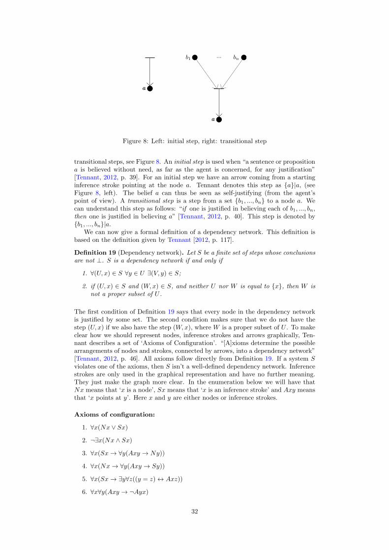
Figure 8: Left: initial step, right: transitional step

transitional steps, see Figure 8. An initial step is used when “a sentence or propositiona is believed without need, as far as the agent is concerned, for any justification”[Tennant, 2012, p. 39]. For an initial step we have an arrow coming from a startinginference stroke pointing at the node a. Tennant denotes this step as {a}|a, (seeFigure 8, left). The belief a can thus be seen as self-justifying (from the agent’spoint of view). A transitional step is a step from a set {b1, ..., bn} to a node a. Wecan understand this step as follows: “if one is justified in believing each of b1, ..., bn,then one is justified in believing a” [Tennant, 2012, p. 40]. This step is denoted by{b1, ..., bn}|a.

We can now give a formal definition of a dependency network. This definition isbased on the definition given by Tennant [2012, p. 117].

Definition 19 (Dependency network). Let S be a finite set of steps whose conclusionsare not ⊥. S is a dependency network if and only if

1. ∀(U, x) ∈ S ∀y ∈ U ∃(V, y) ∈ S;

2. if (U, x) ∈ S and (W,x) ∈ S, and neither U nor W is equal to {x}, then W isnot a proper subset of U .

The first condition of Definition 19 says that every node in the dependency networkis justified by some set. The second condition makes sure that we do not have thestep (U, x) if we also have the step (W,x), where W is a proper subset of U . To makeclear how we should represent nodes, inference strokes and arrows graphically, Ten-nant describes a set of ‘Axioms of Configuration’. “[A]xioms determine the possiblearrangements of nodes and strokes, connected by arrows, into a dependency network”[Tennant, 2012, p. 46]. All axioms follow directly from Definition 19. If a system Sviolates one of the axioms, then S isn’t a well-defined dependency network. Inferencestrokes are only used in the graphical representation and have no further meaning.They just make the graph more clear. In the enumeration below we will have thatNx means that ‘x is a node’, Sx means that ‘x is an inference stroke’ and Axy meansthat ‘x points at y’. Here x and y are either nodes or inference strokes.

Axioms of configuration:

1. ∀x(Nx ∨ Sx)

2. ¬∃x(Nx ∧ Sx)

3. ∀x(Sx→ ∀y(Axy → Ny))

4. ∀x(Nx→ ∀y(Axy → Sy))

5. ∀x(Sx→ ∃y∀z((y = z)↔ Axz))

6. ∀x∀y(Axy → ¬Ayx)

32

7. ∀x∀y((Sx ∧ Sy)→ ∀z((Axz ∧Ayz)→ (∀w(Awx→ Awy)→ (x = y))))

8. ∀x(Nx→ ∃yAyx)

Let us now look at the dependency network in a more informal way. Let ushave a finite set of nodes N = {b1, ..., bn}, representing all the beliefs in your beliefsystem before having deduced anything. Let M = {b1, ..., bm}, m < n, be a subsetof N that forms a set of beliefs which are used as premises for some conclusion a.The corresponding nodes can be white or black. From all the nodes in this subsetthere is an arrow pointing at an inference stroke which is also white or black. Theinference stroke is black if all the nodes pointing at it are black and the inferencestroke is white if at least one node corresponding to an element of the set M is white.From the inference stroke there is an arrow pointing at the conclusion a. The nodecorresponding to a is white if the inference stroke is white and black if the inferencestroke is black. Thus, as soon as a rational agent does not believe one of his premisesanymore, he is obliged to stop believing the conclusion. This means that believingthe premises is necessary for believing the conclusion.

Note that it doesn’t matter whether beliefs are true or not. We only talk aboutwhether something is believed by a rational agent. Every rational agent has his ownbeliefs and draws his own conclusions from it. An agent can believe that b1, ..., bk,k < n, are necessary to believe a. But, in the real world it can be possible that b1is not necessary at all for a to be true. The rational agent is just not aware of theexistence of this step. Here, read the words ‘true’ and ‘believe’ carefully. Everythinggoes well, as long as the agent does not ignore the fact that if he believes all premisesof a set M and he is aware of the step from these premises to a, he must believe a aswell. If he ignores this fact, he is not a rational agent.

According to Tennant, the actual system of beliefs are only the black nodes andthe black inference strokes. They form a subsystem (or subnetwork) R in the totalsystem S, that is, R is also a dependency network and has to satisfy all the axiomsof configuration. This system R is a closed system, which means that R is equal toits closure.

Definition 20 (Closure). The closure R of a subsystem R ⊆ S is the smallest sub-system in S such that the following two properties are satisfied:

1. R is a subsystem of R;

2. if for every step in S it holds that if the premise set {b1, ..., bm} is in R, thenthe step {b1, ..., bm}|a is in R.

Tennant gives another set of axioms, called ‘Axioms of Coloration’. These axiomsdescribe how the nodes and inference strokes should be colored. They follow directlyfrom Definition 20. If one of these axioms of coloration is violated we would havethat R is not closed, that is, R 6= R. In the following enumeration we have that Bxmeans ‘x is black’ and Wx means ‘x is white’.

Axioms of coloration:

1. ∀x((Bx ∧Nx)→ ∃y(By ∧ Sy ∧Ayx))

2. ∀x((Wx ∧Nx)→ ∀y(Ayx→ (Wy ∧ Sy)))

3. ∀x((Bx ∧ Sx)→ ∀y(Ayx→ (By ∧Ny)))

4. ∀x((Wx ∧ Sx ∧ ∃zAzx)→ ∃y(Wy ∧Ny ∧Ayx))

A more detailed explanation of these axioms can be found in [Tennant, 2012, p.47-50]. In Figure 9 violations of the four axioms of coloration are given. The numbersin the figure correspond to the numbers of the axioms of coloration. The first and

33

Figure 9: Violations of the four axioms of coloration.

second axiom are of the same type and are violated, because the conclusion node andthe inference stroke pointing at it do not have the same color. The third axiom isviolated, because an inference stroke can only be black if all premise nodes pointingat it are black. The fourth axiom is violated in a similar way as the third.Thus, if we would have a violation of an axiom of configuration, then we cannot speakof a well-defined dependency network and if one of the axioms of coloration is violatedwe would have that R is not closed.

Finally, according to Tennant, the geometry of the system is static. This meansthat the arrows connecting nodes with inference strokes cannot change and there cannot be new nodes, inference strokes or arrows added to the network. The only thingsthat change are the colors of nodes and inference strokes. This is what the bookChanges of Mind is about, changing your beliefs. This will be explained next.

7.2 The contraction problem

Having explained Tennant’s belief system, we can show what he means with the con-traction problem. It is a problem about changing your mind. Contraction means thatan agent gives up one or more beliefs (make a black node white), whereas expansionmeans that the system is expanded with a new belief (color a white node black). Con-traction and expansion together form belief revision, but the step of belief expansionis relatively simple. Therefore, Tennant talks about the problem of contraction.

Contracting a system with respect to a node a means that a rational agent re-moves a from his actual belief system, that is, the agent doesn’t believe a anymore.But you cannot just remove a from the belief system, because then the system isn’tclosed anymore. The premise set {b1, ..., bm} is still in R which implies that the step{b1, ..., bm}|a must be in R. But, since a is not in R anymore, a is not in R andtherefore the step {b1, ..., bm}|a is not in R anymore. This means that the agent isobliged to stop believing at least one of the premises b1, ..., bm, say for example b1.Then the agent has to check what the consequences are of not believing b1 anymore.He should check whether the remaining system is closed or not until he reaches aninitial step. This is called the contraction problem. Tennant wants this problem tobe “as economical as possible, in the sense that one gives up as little as possible”[Tennant, 2012, p. 130] when contracting the system from S to S − a. He calls thisthe ‘minimal mutilation’ condition. The contraction problem can be stated as thefollowing decision problem.

Given a finite belief system S containing the belief a and an integerK < |S|. Does there exist a contraction of the system with respect toa of at least size K?

In other words, does there exist a subsystem R ⊆ S, not containing a, of size at leastK? Tennant also gives a more formal definition of the problem.

34

Given a finite belief system S containing the belief a and an integerK < |S|. Does there exist a closed subsystem R of at least size K thatdoes not contain a?

According to Tennant, this decision problem is NP-complete. Indeed, there aredifficulties in the contraction problem which cannot be deterministically computed inpolynomial time. We can only find out by trial and error whether there is a contractionof at least size K that does not contain a. Just try all possible subsystems of at leastsize K to check whether these subsystems are closed and do not contain a. Thiswill give us a problem of at least order O(2|S|), because the system is of size |S|and for each step in S we have two possibilities: either the agent believes the stepor he doesn’t. Thus, the number of possibilities is exponential. Hence, Tennant’scontraction problem is not in P. But it is in NP. If we are given a system S and R ⊆ Sa subsystem of a least size K, then we can check in polynomial time whether R doesnot contain a and whether R is closed in S. Checking whether R does not containa is easy, because we only have to walk through the system and check whether a iscontained or not. This can be done in linear time, bounded by the size of R. Accordingto Tennant we can check in polynomial time whether R is closed in S. Rememberthat R is a set of steps and we must check that R = R. Thus, for every step in Rwe must check whether all premises are believed, and if so, then the conclusion hasto be believed too. This means we have to run c · |R| times through the steps inR, where c is a positive constant. Thus, we can check in polynomial time of orderO(|R|2) whether R is closed in S. Therefore, the contraction problem is in NP. Inhis book, Tennant proves the NP-completeness of the contraction problem by givinga reduction from Vertex Cover to it [Tennant, 2012, p. 133-134].

Having explained how Tennant’s belief system and contraction problem work wewill look at two aspects of the book. We discuss whether the belief system is a realisticrepresentation of the mind. This is done according to the fact that the geometry of thesystem is static. We also discuss whether we can say something about the complexityof a problem about the mind.

7.3 How realistic is Tennant’s belief system?

We ended 7.1 by saying that, according to Tennant, the geometry of the system wasstatic. With this he meant that the only things that can change in the dependencynetwork are the colors of the nodes and inference strokes. There is no way to addanything new to the network. If Tennant meant to represent human beings with thelogical paragon, then the belief system is not very realistic. If there is no way to addnew steps to the network, how is it possible to learn new things? And when in lifewill the geometry of the system be fixed? Is the geometry fixed as soon as we areborn or can it be fixed at any moment in life? Or do we assume that the systemcontains every belief there is to know? All options sound strange given the fact thatthe system is static. Fixing a belief system at birth, suggests that the geometry of asystem is the same for everyone, because the system does not contain any beliefs yet,the dependency network is empty. According to Tennant we cannot add things to thenetwork, which leaves us with a system without beliefs. This is not a fine prospectfor mankind.

Then there is the option of fixing the geometry of a belief system at any momentin life. Every individual agent has a different system built up from his own beliefsuntil that moment. Within the system, changing a belief can be done by making ablack node white. But if we observe and learn new things, what will happen to thesystem? For example, you are shopping with your friend and she shows you a sweaterwhich she likes very much. You see the sweater for the first time and you believe thatit looks good on her. This is a new belief, a black node. According to Tennant weneeded a white node first to transform it into a black node. But, in a static systemthere is no possibility to add a new node to the system, even if the belief that youliked the sweater was really in your mind. How do we learn new things? Instead of

35

fixing the geometry of the system at birth, fixing the geometry at the end of your lifecould be an option, so that the system is complete. But what is the point of changingyour mind if you are about to die? Thus, the option of fixing the geometry of thebelief system at any moment in life is not realistic.

The third option to learn new things is to accept the assumption that the systemcontains every belief there is to know. Every rational agent can color it accordingto his beliefs. But, it is impossible for humans to have a belief system containingevery possible belief, because nobody has complete knowledge about the world. Weknow that Tennant describes a belief system as a set of steps which are all known tothe rational agent, thus, even the white nodes in the dependency network have to beknown to the agent. In this way an agent can check for example whether he believesp or ¬p. If it would be the case that the system contains every belief in the world,then the system is probably not finite anymore. If the system would become infinitelylarge, we could only work with it if we were logical saints. Tennant wants to avoidthis by introducing the logical paragon. Therefore, the option that we could onlylearn new things if the belief system contains every belief, is not the option Tennanthas in mind.

The most realistic option could be that the system is fixed every time a belief ischanged. If an agent changes a belief p into ¬p, then the system is refreshed beforechanging of belief again. If the agent then makes up his mind once more, the systemis fixed again and so on. This still doesn’t explain how to learn new things. Newthings simply appear in the system and are related immediately to the rest of thesystem. This is something a logical paragon can, but humans can’t. The idea oflearning new things might be an NP-complete (or even harder) problem itself andTennant separates these two problems. He doesn’t mention that these problems arevery closely related. The geometry of Tennant’s belief system is indeed static, which isuseful for showing that the contraction problem is NP-complete, but it is not realistic.You cannot separate belief change from learning new things. Humans often changetheir mind because they learn a new belief which, for example, contradicts an oldbelief. The system should be a more dynamic system, but then the problem becomestoo hard to solve.

Next, we will discuss whether we can speak of the computational complexity of aproblem about belief change.

7.4 Can you say something about the complexity of a problemabout the mind?

We have seen that the contraction problem of Tennant is NP-complete. Does thismean that Tennant says that we are solving NP-complete problems in our mind?And why does Tennant want his problem to be NP-complete?

The contraction problem of Tennant is NP-complete. This means that a computercannot solve the problem deterministically in polynomial time, but there is an algo-rithm that can guess a solution and can verify in polynomial time if this is indeeda solution. Tennant has placed a lot of restrictions that make the problem easier tosolve, but also less realistic. For example, the fact that the geometry of his depen-dency network is static is not very realistic, but makes the problem look very similarto other decision problems with graphs (e.g. TSP, CLIQUE, VC). Therefore, Ten-nant can reduce Vertex Cover to the contraction problem. Another restriction is thatevery object and structure Tennant works with is finite. It can be the case that thereare infinitely many beliefs, but according to Tennant a rational agent never believesmore than finitely many of them. If the belief system would contain infinitely manysteps there is no possibility that the contraction problem is NP-complete or evencomputable. Thirdly, Tennant has restricted the problem to just looking whethera belief is justified by the agent. He doesn’t look at the logical structure within abelief. If he looked at the logical structure, the problem would become more compli-cated. Probably because of all the restrictions, the contraction problem has become

36

NP-complete.Tennant thinks that it is useful that the contraction problem is NP-complete. If

Tennant means to represent humans with the logical paragon, then in a way he saysthat we are solving NP-complete problems in our mind. He formally represents in abelief system what is happening in the mind of an agent (our mind) when changinga belief. By solving the contraction problem exactly Tennant proves that this isan NP-complete problem. Are we continuously solving NP-complete problems whenchanging our mind? No we aren’t. But if something that happens in our mind isNP-complete for a computer, how can it be that we have no problems when we arechanging our beliefs? Suppose you are given an arbitrary instance of size n of theTraveling Salesman Problem and you are asked to check whether there exists a tourwith costs less than K. You cannot easily solve this decision problem and it is neithersomething we do all day long. If the instance is small, say n = 4, we can solvethe problem. As soon as the instances become larger, we aren’t capable of solvingit exactly, but we can sometimes make a good guess of what the answer should be.Guessing is something humans are good at, in contrast to computers. Our guessing isbased on rational thinking, whereas computers guess randomly, based on an algorithmtogether with a whole set of data.

The same idea works for the contraction problem where we change a belief (as-suming that Tennant still wants to represent humans with his logical paragon). Whenwe contract the belief system with respect to a belief p, we remove p from the system.The color of p changes from black to white. A logical paragon can check in polyno-mial time whether the remaining system is still a closed subnetwork of at least sizeK. But we, humans, do not check directly whether everything we believe still holdsafter a contraction. We don’t check our memory step by step on every belief. Wejust stop believing p, because we observed the opposite of p or we stopped believingone of the premises necessary for believing p. There are many reasons why we couldstop believing p and we don’t always think about the consequences that a contractionmight have. It could be that after ten years we still believe something for which it wasnecessary that we believed p. Tennant assumes with the contraction problem that arational agent knows directly what he can and cannot believe after contracting withrespect to p. If this assumption is correct, an agent had to check all of his memoryevery time there was a contraction and he would be busy with doing this for ever.There would be no time to think about other things, because his memory is constantlybusy with computing. Changing our beliefs is something we are doing multiple timesa day, which means that if we were represented by the logical paragon we would bebusy with changing our beliefs for the rest of our life. To refer to Tennant’s depen-dency network: humans would probably only check the nearby beliefs in the networkwhich can be thought of as a small subnetwork. This smaller subnetwork can be seenas a small instance which we can solve. We are capable of solving small instances ofNP-complete problems as long as we can visualize them. As soon as the instancesbecome larger or the problem is generalized for arbitrary n, we can only guess ananswer. We saw that humans are good at guessing in contrast to computers.

Thus, there is a possibility that we can solve NP-complete problems for smallinstances. But we don’t seem to have problems with doing this. We sometimeseven find a solution instead of only the yes/no-answer that a computer gives. Acomputer can only verify in polynomial time whether a given instance is a solutionto the problem, but he cannot find a solution to a problem in polynomial time. Forsmall instances we often produce an answer faster than a computer. This is becausea computer needs an algorithm together with all data to ‘understand’ the problemand the mind only needs frames of the most relevant beliefs and fills in the details.We don’t run through our whole memory to check whether there is a contradictionin our beliefs. For example, if you are changing your mind about whether it rains ornot, there is no reason to look at the beliefs about whether you like the color of asweater. We only search through the beliefs of which we intuitively think that theyare relevant and a computer needs to search the whole set of beliefs. Maybe the mind

37

uses a faster algorithm than a computer or maybe we don’t use an algorithm at alland are we just doing what seems best to do at that moment.

Another fact is that we are even solving problems with our mind which a computercan’t solve. For example, checking the validity of an argument in first order logic. Anargument is valid if its conclusion follows logically from is premises. First order logicdiffers from propositional logic, because of the use of the quantifiers ‘∀’ and ‘∃’. Theproblem of checking whether a formula is valid can be undecidable for a computer(in fact it is semi-decidable, but we will not elaborate on this). We are able to solvethis problem for small instances. This means that we are capable of a lot more thanwe can imagine. If we ever discover how our mind solves such problems, we mightbe able to solve them for arbitrary n. But for this to happen we have to wait a longtime, maybe even infinitely long.

Tennant writes about the complexity of a problem about the mind. He thinks it isuseful and important that his contraction problem is NP-complete. Tennant believesthat we are one step further in the search if our mind can be seen as a computationalobject. By using a computer Tennant tries to show what, according to him, happensin the mind of a rational agent when this agent changes his beliefs. But, we saw beforethat Tennant’s belief system was not very realistic, because not even a logical paragonhas knowledge about all beliefs, and is therefore not capable of learning new things.This means that it is neither the mind of a logical paragon that is represented by acomputer nor the mind of a human. Changing beliefs is much more complicated thenTennant says. We probably need more to represent the mind. Humans don’t alwaysbehave like rational agents. Sometimes humans just ignore the fact that they believecontradictory things. Here we enter the discussion about whether humans have ‘freewill’, but this lies outside the scope of this thesis. It is impossible to separate the partwhere we change our beliefs from the rest of our mind. To link the two themes ‘mind’and ‘complexity’ to each other in the way Tennant does, is not helpful in searchingwhether our mind can be seen as a computational object.

38

8 Conclusion

In this thesis we focused on several decision problems and we proved polynomial reduc-tions between them. The decision problems we looked at were SAT, 3-SAT, CLIQUE,Vertex Cover, Hamiltonian Circuit and TSP. These were introduced in Sections 3 and4. Before proving these reductions we defined in Section 5 the complexity classes P,NP and NP-complete. We also needed a definition of a polynomial reduction and weproved in Lemma 1 the transitivity of a polynomial reduction. We ended Section 5with showing that the decision problem 3-SAT is NP-complete by reducing SAT to it.In Section 6 we proved step by step that SAT can be reduced to TSP. We started thisproject with the goal to find out whether a direct polynomial transformation functionfrom SAT to TSP could be found. It is possible in theory, because we know of bothproblems that they are NP-complete. Unfortunately we only found the compositionof the reductions in between SAT and TSP. We have shown these reductions stepby step based on an article written by Karp [1972, p. 97-98]. In his article Karpgave transformations of instances for different NP-complete problems, but he did notprove them. The polynomial reductions we proved were SAT � CLIQUE, CLIQUE �VC, VC � HC and HC � TSP. Having proved this, we could immediately see why weweren’t able to find a direct reduction from SAT to TSP. The resulting graph becomesreally complicated for only a simple Boolean formula. It is difficult to discover whatthe original Boolean formula was in the resulting graph. This is mainly because oftwo things. When reducing CLIQUE to Vertex Cover we took the complement and byreducing Vertex Cover to Hamiltonian Circuit, we looked at edges instead of nodes.These things lead to some confusion when trying to reduce SAT directly to TSP. It isa nice puzzle to try and find a direct reduction from SAT to TSP, but for this thesisit took too much time.

The second part of this thesis, Section 7, was about a more philosophical decisionproblem. We gave some remarks on a contraction problem proven to be NP-completeby Neil Tennant in Changes of Mind. The book is about changing your beliefs in abelief system. We described Tennant’s belief system and contraction problem. Thenwe have discussed how realistic this belief system is and concluded that it is not veryrealistic that the geometry of his system is static. This meant that nothing couldbe added to the system, which immediately lead to the question how we learn newthings. Tennant probably sees this as a different problem, but he doesn’t mentionthat they are closely related.

We discussed whether we can say something about the complexity of a problemabout the mind. We saw that the contraction problem of Tennant was NP-complete,but does this mean that he says that we are solving NP-complete problems in ourmind? A logical paragon can check in polynomial time whether the remaining systemis still a closed subnetwork of at least size K. But we, humans, do not check directlywhether everything we believe still holds after a contraction. We don’t check ourmemory step by step on every belief. Humans would probably only check the nearbybeliefs in the network which can be thought of as a small subnetwork. This smallersubnetwork can be seen as a small instance which we can solve. We are capable ofsolving small instances of NP-complete problems as long as we can visualize them. Assoon as the instances become larger or the problem is generalized for arbitrary n, wecan only guess an answer. Therefore, to link the two themes ‘mind’ and ‘complexity’to each other in the way Tennant does, is not helpful in searching whether our mindcan be seen as a computational object.

39

References

M. H. Alsuwaiyel. Algorithms: Design techniques and analysis, volume 7 of Lecturenotes series on computing. World Scientific Publishers, 1999.

G. Boole. An investigation of the laws of thought: On which are founded the mathe-matical theories of logic and probabilities. Walton and Maberly, London, 1854.

S. Dasgupta, C. H. Papadimitriou, and U. V. Vazirani. Algorithms. McGraw-Hill,2006.

R. Gamboa and J. Cowles. A mechanical proof of the Cook-Levin theorem. InK. Slind, A. Bunker, and G. Gopalakrishnan, editors, Theorem proving in higherorder logics, pages 99–116. Springer, 2004.

Jiahong Guo and Lei Zhang. Book review of Changes of mind: An essay on rationalbelief revision by Neil Tennant. Notre Dame philosophical reviews, 2013.

D. R. Hofstadter. Godel, Escher, Bach: An eternal golden braid. Basic Books, UnitedStates of America, 1979.

D. S. Johnson and M. R. Garey. Computers and intractability. W. H. Freeman andCompany, New York, 1979.

R. M. Karp. Reducibility among combinatorial problems. In R. E. Miller and J. W.Thatcher, editors, Complexity of computer computations, pages 85–103. Springer,New York, 1972.

C. H. Papadimitriou. Computational complexity: A guide to the theory of NP-completeness. Addison-Wesley Publishing Company, Massachussetts, 1994.

W. Pohlers and T. Glaß. Lecture notes of the course an introduction to mathematicallogic. Wilhelms-Universitat Munster, 1992.

G. Schafer. Lecture notes of the master course discrete optimization, Utrecht Univer-sity, 2012.

N. Tennant. Theory-contraction is NP-complete. Logic Journal of the IGPL, 11:675–693, 2003.

N. Tennant. Changes of mind: An essay on rational belief revision. Oxford UniversityPress, Oxford, 2012.

J. P. Warners. Nonlinear approaches to satisfiability problems. PhD thesis, EindhovenUniversity of Technology, 1999.

40