ghana - wp - will it be cursed or gifted-redline copy will it be gifted or will it be cursed?...

WP/11/104

Ghana: Will It be Gifted or Will It be Cursed?

Burcu Aydin

© 2011 International Monetary Fund WP/11/104 IMF Working Paper African Department

Ghana: Will It be Gifted or Will It be Cursed?

Prepared by Burcu Aydin

Authorized for distribution by Peter Allum

May 2011

This Working Paper should not be reported as representing the views of the IMF. The views expressed in this Working Paper are those of the author(s) and do not necessarily represent those of the IMF or IMF policy. Working Papers describe research in progress by the author(s) and are published to elicit comments and to further debate.

Abstract

Will Ghana’s oil production from 2011 accelerate progress toward middle-income status, or will it retard gains in living standards through a possible “resource curse”? This paper examines the likelihood of “resource curse” effects, drawing on a dataset of 150 low and middle income countries from 1973 to 2008 using static and dynamic panel estimation techniques. Results confirm that resource rich countries in Ghana’s income range do experience slower growth than their more diversified peers, an effect that appears to be related to weaker governance. Provided that Ghana can preserve and improve its economic governance and also strengthen fiscal management, prospects look good for converting its oil wealth into sustained strong economic growth. JEL Classification Numbers: C33, O10 Keywords: Ghana, growth, resource-rich, panel data Author’s E-Mail Address: [email protected]

2

Table of Contents I. Introduction: .......................................................................................................................... 4 II. Data: ..................................................................................................................................... 5 III. Are Resource-Rich Countries Cursed? ............................................................................... 8

A. Introduction ...................................................................................................................... 8 B. Methodology .................................................................................................................. 10 C. Results ............................................................................................................................ 11 D. Robustness ..................................................................................................................... 14

IV. Impact of Macroeconomic and Structural Policies ........................................................... 15 A. Introduction and Methodology....................................................................................... 15 B. Results ............................................................................................................................ 16

V. And It is the Institutions That Matter ................................................................................. 18 A. Introduction and Methodology....................................................................................... 18 B. Results ............................................................................................................................ 19

VI. What Does It Imply for Ghana? ........................................................................................ 22 A. Where Does Ghana Stand Within the LMIC? ............................................................... 22 B. Where Will Ghana Be in 2014 ....................................................................................... 26

VII. Conclusion ....................................................................................................................... 28 VIII. Bibliography ................................................................................................................... 29 Appendix ................................................................................................................................. 31

A. Unit Root Test Results ................................................................................................... 32 B. Correlation across Variables of Interest ......................................................................... 40

3

Tables Table 1. Summary Statistics for the Common Estimation Sample ........................................... 7 Table 2. Growth of Resource-Rich and Diversified LMICs 1/ ................................................. 9 Table 3. Growth Regression Results ....................................................................................... 12 Table 4: Estimated Growth at Different Initial Income Levels 1/ .......................................... 13 Table 5. The Impact of Macroeconomic and Structural Variables on Economic Growth ..... 16 Table 6. Estimated Growth Impact of the More Richly Specified Model .............................. 17 Table 7. The Impact of Institutional Quality on Economic Growth ....................................... 20 Table 8. Macroeconomic Indicators for Ghana ...................................................................... 23 Table 9. Governance and Fiscal Indicators for Ghana ............................................................ 24 Table 10. Structural Indicators for Ghana ............................................................................... 26 Table 11. Panel Unit Root Test Result for Relative Economic Growth ................................. 32 Table 12. Panel Unit Root Test Result for Relative Income per Capita ................................. 32 Table 13. Panel Unit Root Test Result for Openness ............................................................. 33 Table 14. Panel Unit Root Test Result for REER ................................................................... 33 Table 15. Panel Unit Root Test Result for Terms of Trade .................................................... 34 Table 16. Panel Unit Root Test Result for Fiscal Balance-to-GDP ........................................ 34 Table 17. Panel Unit Root Test Result for Old Age Dependency .......................................... 35 Table 18. Panel Unit Root Test Result for Population Growth .............................................. 35 Table 19. Panel Unit Root Test Result for Voice and Accountability .................................... 36 Table 20. Panel Unit Root Test Result for Rule of Law ......................................................... 36 Table 21. Panel Unit Root Test Result for Regulatory Quality .............................................. 37 Table 22. Panel Unit Root Test Result for Political Stability ................................................. 37 Table 23. Panel Unit Root Test Result for Government Effectiveness .................................. 38 Table 24. Panel Unit Root Test Result for Control of Corruption .......................................... 38 Table 25. Panel Unit Root Test Result for Armed Conflict .................................................... 39 Table 26. Pairwise Correlation across Variables of Interest ................................................... 40

Figures Figure 1. Real Per Capita GDP Growth of Resource-Rich and Diversified economies ........... 8 Figure 2. Economic Convergence versus Divergence ............................................................ 11 Figure 3. Governance Indicators for Ghana ............................................................................ 25 Figure 4. Decomposition of Growth for Ghana ...................................................................... 27

4

I. INTRODUCTION

Ghana has discovered offshore oil wealth, which should come on stream in 2011. Ghana’s share of export revenues is projected at around 6-7 percent of GDP over a 5- to 10-year period, falling gradually thereafter. But new discoveries are being announced, and the level and duration of oil income could increase. A much-debated policy issue is to what extent economic growth and living standards in Ghana can be expected to improve as a result of the move to oil producer status. On the one hand, oil revenues relax external and fiscal constraints. If oil incomes are invested prudently—whether in improved infrastructures, or in better education or health—this would be expected to boost incomes and living standards. Against this, many resource-based countries have not seen strong growth, and living standards have stagnated. This provides a cautionary note as to the likely impact of Ghana’s oil wealth. There are three broad strands to the literature on the impact of natural resources on economic growth. A first group of papers supports the concept of a resource curse, with resource-rich countries observed to grow less rapidly than their peers. In an early paper, Prebisch (1959) argued that weak growth in Latin America reflected the limited possibilities for technological growth for natural resource industries. Both Neumayer (2004) and Mehlum et. al. (2006) support the concept of a resource curse, noting the slower growth of resource-rich countries since the 1960s. Gylfason and Zoega (2001) argue that physical capital may be crowded out in resource-rich countries, slowing down their economic growth. Sachs and Warner (2001) analyze whether previously omitted geographical and climate variables can explain the resource curse, and find little evidence on that or any bias resulting from other unobserved growth deterrents; and further conclude that resource-abundant countries in general are high-price economies and hence they miss-out on export-led growth. A second strand of literature argues the opposite—that resource-rich countries are blessed, growing faster than non-resource countries. In this literature, Lederman and Maloney (2007) argue that natural resources promote growth when combined with accumulation of knowledge. Doppelhofer et. al. (2000) show that mining production as a share of GDP is a robust predictor for higher economic growth when analyzed by bayesian averaging methods. In a third strand of literature, researchers question whether natural resources have any significant impact on countries’ growth paths. Stijns (2005) shows that natural resource abundance has not been a significant structural determinant of economic growth. Davis (1995) questions the resource-curse hypothesis in a larger scale of cross-country data, and finds little evidence supporting this hypothesis. Manzano and Rigobon (2001) show that, after controlling for initial levels of foreign debt relative to GDP, the negative correlation between natural resources and growth disappears (Sachs & Warner, 2001). This paper studies the impact of natural resources on growth, and the main contribution of this paper to the literature is on two folds. First, the paper is one of the few analyses, which

5

gathers a numerous dataset for low- and middle- income countries (LMIC). The panel dataset starts from 1970s and contains 150 LMICs, comprised of both resource-rich and diversified economies. Second, the paper contributes to the growth impact of resource wealth literature by acknowledging the difference between institutional backgrounds of LMICs. The paper incorporates a rich dataset on institutions covering both governance and stability across LMICs. In order to analyze this rich dataset, we employ static and dynamic panel estimation methods. We test whether resource-rich countries on average grow more slowly than non-resource countries by controlling for macroeconomic, structural and institutional variables. On the macroeconomic side, indicators for initial income levels, openness, and competitiveness are explored, while structural and institutional effects are considered in regard to demographics, the quality of economic governance, checks and balances on governance, and political stability. Results show that there is a poverty trap for poor resource-rich countries due their low institutional quality. Notwithstanding this, resource wealth can boost growth if supported with strong governance and good macroeconomic management. We show that for Ghana, a country with relatively strong institutions, oil wealth could boost its per capita income growth by up to 2 percentage points in the long-run, if macroeconomic policies are also strengthened by reducing the fiscal deficit in line with current plans. In what follows, Section II introduces the data. Section III analyzes the impact of income and resource wealth on the growth path. Section IV studies the impact of macroeconomic and structural policies and Section V the institutional structure on the growth rate of an economy. Then, Section VI applies the findings from the preceding section to Ghana. Last, Section VII draws conclusions.

II. DATA

Data are drawn from an annual unbalanced panel dataset of 150 LMICs from 1973 through 2014. The dataset up to 2009 is based on realized historical data, and this section is used for model estimations, and the remaining five years are IMF Staff’s projections and these are used for forecasting purposes in Section VI. Macroeconomic variables for this dataset are obtained from the World Economic Outlook (International Monetary Fund, 2009). Variables on demographics are obtained from the World Bank’s World Development Indicators database. Effective exchange rate and trade weight data are from the IMF Information Notice System; and net foreign asset data are from the IMF Balance of Payments database.1

1 The dataset was adjusted in a number of ways. The following are treated as data errors and excluded from the estimation sample: negative values for nominal GDP, GDP at constant prices, government consumption, exports, imports, population, employment, exchange rate, and terms of trade; and absolute values greater than 100 percent for dependency ratio, population growth, and for fiscal balance, government spending, current account balance and trade balance as a percent of GDP. Trade weight data are replaced by the data reported by country authorities whenever there is a large discrepancy.

6

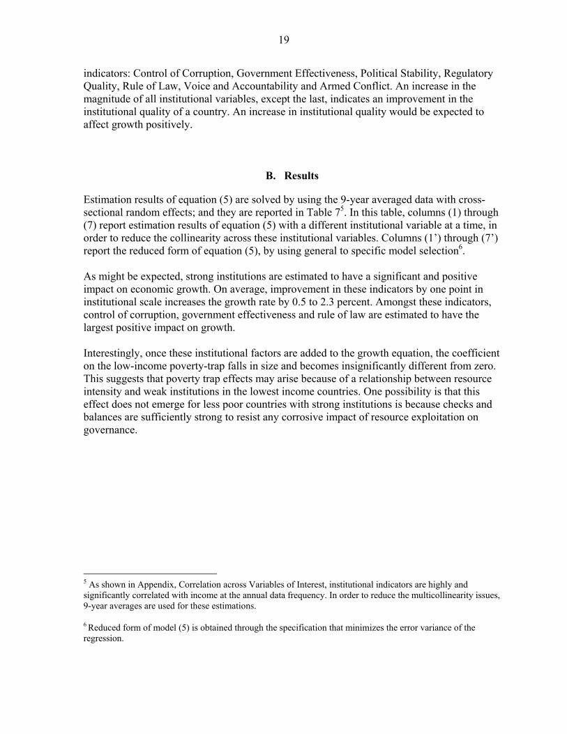
Data on institutional indicators are obtained from the Worldwide Governance Indicators dataset (World Bank, 2009) (see Box 1 below), while data on armed conflict are from the Uppsala Conflict Data Program (2009).

Box 1. Governance Indicators

The governance indicators reported in Table 1 cover the period from 1996 to 2008. Country values range from -2.6 to 1.5, with higher magnitudes indicating better governance. This paper examines six measures of governance:

Control of Corruption: the extent that public power is exercised for private gain;

Government Effectiveness: the quality of public services and policy formulation, capacity of civil service and its independence from political pressure.

Political Stability: the likelihood of a government becoming destabilized by unconstitutional or violent means.

Regulatory Quality: the capacity of a government to provide sound policies and regulations which would promote private sector development.

Rule of Law: the confidence of citizens in law, and the extent that they abide by the rules of the society, such as contract enforcement, property rights, police, and courts

Voice and Accountability: the degree of capacity of a country’s citizens in selecting the government, and freedom of expression, freedom of association and free media

Countries are classified as resource-rich based on their main exports, as reported in the IMF’s World Economic Outlook (Appendix A). Of the 150 low- and middle-income countries, 45 are classified as resource-rich. Of this total, 26 countries are classified as fuel exporters, with around half coming from the Middle East, and a little less than one third from Africa. The remaining 19 countries export other primary commodities, with more than half representing African countries. Table 1 provides summary statistics for the variables of interest obtained from the common estimation sample. Statistics show that average growth rate for the LIMC was at 5 percent; however, there is a high variance across these countries, of 5 percent standard deviation, ranging from a negative of 33 percent to a maximum of 86 percent. Initial real income per capita for the LIMC countries was around 3,400 US dollar, again with a high variation amongst these countries of around 3,000 US dollars per standard deviation.

7

Table 1. Summary Statistics for the Common Estimation Sample

Min. Mean Max. Std. Dev. Skewness Kurtosis

Per Capita Growth1 -0.33 0.05 0.86 0.05 2.21 41.22

Resource2 0.00 0.30 1.00 0.46 0.89 1.79

Fuel2 0.00 0.13 1.00 0.34 1.79 4.20

Initial Income3 -1.20 1.22 4.45 1.10 -0.03 2.28

REER3 -1.49 -0.01 1.47 0.24 -1.24 14.60

Imports/GDP 0.00 0.47 6.28 0.29 6.45 115.62

Terms of Trade3 -0.95 0.00 0.87 0.22 -0.13 6.10

Fiscal Balance/GDP -0.49 -0.02 0.43 0.07 1.29 15.33

Control of Corruption -1.76 -0.35 1.51 0.66 0.54 2.72

Government Effectiveness -1.88 -0.32 1.49 0.66 0.31 2.55

Political Stability -2.61 -0.27 1.40 0.83 -0.35 2.57

Regulatory Quality -2.44 -0.25 1.58 0.75 -0.15 2.76

Rule of Law -1.88 -0.36 1.40 0.71 0.30 2.28

Voice and Accountability -2.24 -0.32 1.46 0.84 -0.01 2.07

Armed Conflict2 0.00 0.17 1.00 0.37 1.78 4.16

Old Age Dependency4 0.01 0.09 0.26 0.05 1.51 4.41

Population Growth1 -0.17 0.02 0.26 0.02 2.13 39.92

Notes: Number of observations drawn from the common sample is 1543. 1: Calculated from the log-difference. 2: 0-1 indicator variable. 3: in logs: REER and terms of trade ratioed by 100, and income in thousands of US dollar. 4: is the ratio of retirees to working age population (= age 65+ / ages 16 to 65] )

Regarding the stationarity of the variables of interest, panel unit root test statistics are provided in the Appendix B, Unit Root Test Results. Based on these statistics, none of the variables have a unit root that cannot be rejected by a majority of the test results.

Last, for refraining from the impact of multicollinearity on the regression coefficients, pairwise correlation coefficients within variables of interest are reported in Appendix C,

8

Correlation across Variables of Interest. Results show high and significant correlation across governance indicators, and between the governance indicators and income.

III. ARE RESOURCE-RICH COUNTRIES CURSED?

A. Introduction

In this paper, the first question that we will study is whether resource-rich countries are cursed, or in other words, whether these countries grow less than other economies on average. To illustrate this point, Figure 1 plots the average real per capita GDP growth rate of the resource-rich and diversified economies from 1990 to 2008, controlling for the initial real income per capita.

Figure 1. Real Per Capita GDP Growth of Resource-Rich and Diversified economies

Note: y-axis plots the average real per capita income growth over the 1990s and 2000s.

x-axis plots the average real per capita income over the 1970s and 1980s (measured

in thousands of US dollar and in logs)

Equatorial Guinea -a resource rich economy- and Zimbabwe -a diversified economy-

is excluded from the graph as outliers.

y = -0.0042x + 0.0433R² = 0.0405

y = -0.0014x2 + 0.0052x + 0.0368R² = 0.0675

-0.04

-0.02

0

0.02

0.04

0.06

0.08

0.1

0.12

-2 -1 0 1 2 3 4

1990s-2000s

Diversified Economies Resource Rich Economies

Linear (Diversified Economies) Poly. Trend (Resource Rich)

9

The dotted blue line in Figure 1 shows the inverse relationship between trend growth of diversified LMICs and their initial income level. Consistent with the economic growth literature, poorer countries tend to grow faster than the rich, contributing to a gradual convergence of per capita incomes. Per capita income growth rates of resource-rich LMICs in Figure 1 tend to fall below the dotted blue line at low income levels (i.e., in the left hand side of the chart, where per capita incomes are less than $1,000 in purchasing power parity prices). This implies that resource-rich countries grow more slowly than their diversified peers. By contrast, at higher income levels, resource-rich LMICs grow in line with, or perhaps even faster than their diversified peers. As illustrated in Table 2, per capita GDP growth in resource-rich countries with incomes of less than $500 per capita is 3 percentage points less per annum than in diversified countries, a difference that is largely eliminated at higher income levels.

Table 2. Growth of Resource-Rich and Diversified LMICs 1/ Initial income 2/ Diversified Resource-rich Difference < $500 5.7 2.7 -3.0 $500 to <$1,000 3.5 3.3 -0.2 $1,000 to <$5,000 3.9 4.5 +0.6 Over $5,000 4.1 3.5 -0.6

1/ Average per capita income growth, 1990-2008. 2/ Average income per capita in 1973-1989.

One implication of these preliminary findings is the apparent lack of income convergence in resource-rich countries. Resource-rich countries with incomes of less than $500 per capita are estimated to grow by nearly 2 percentage points less per annum than countries with incomes of $1,000-5,000 per capita (Table 2). This suggests a resource-based poverty trap, in which low income resource-rich countries fall increasingly behind their resource-rich and more diversified peers in higher income brackets. Based on Figure 1 and Table 2 we explore several policy questions. First, is there an underlying resource curse (or blessing), independent of incomes? Figure 1suggests that a resource curse may exist, and that it may be limited to the poorest countries. However, this finding may not hold up when a richer group of explanatory factors is considered. Second, we consider the nature of any possible resource curse. Does it constitute a poverty trap that precludes catch-up growth, as suggested by Figure 1and Table 2?

10

B. Methodology

We use panel data analysis models to study the impact of resource wealth on economic growth. Model (1) below provides the panel least squares and model (2) the dynamic generalized method of moments presentation of growth.

* *

, 1 2 , 1 3 , 1 , 1 1 , 2 , ,R ( )Y Y Z EGi t i i t i i t i t i t i t i tG c Y R I Y Y I I

(1)

* *

, , 1 1 2 , 1 3 , 1 , 1 1 , 2 , ,R ( )Y Y Z EGi t i t i i t i i t i t i t i t i tG c G Y R I Y Y I I

(2)

In these equations, Gi,t is the logarithmic growth rate of real income per capita of country i at time t. Ri is a 0-1 indicator variable, which takes value 1, if country i is a resource-rich economy. Yi,t-1 is the initial income measured as the one period lagged value of the logarithm

of real income per capita. *

, 1Y Yi tI is another 0-1 indicator variable, which takes value 1, if

initial income of country i is less than Y*. ,Zi tI and ,

EGi tI are two other indicator variables to

account for the outstanding growth rates of Zimbabwe, a diversified economy with an average growth rate of negative 12 percent during the last two decades, and Equatorial Guinea, a fuel exporting country with average growth rate of positive 20 percent during the same period.

In equations (1) and (2), 1 coefficient will test the existence of a resource curse. If there is a resource curse, then the estimated coefficient of this variable should be significantly smaller than zero. For testing the existence of poverty trap for poor resource-rich economies, we will test

whether the coefficient estimate of 3 is significantly smaller than zero. In other words, the

poorer is a resource-rich country, measured by the widening of the variable *( )Y Y , the

slower that it grows.

Figure 2 visualizes the two hypotheses: 1 0 , for the resource curse; and 3 0 for the poverty trap of the poor resource-rich economies. Poverty line is determined for those economies with initial income less than Y*.

11

Figure 2. Economic Convergence versus Divergence

C. Results

Estimation results of equations (1) and (2) are reported in the first two columns of Table 32. And these results provide some support for both an underlying resource curse as well as a low-income poverty trap effect. However, the latter effect dominates, and the resource curse is significantly different from zero only at the 20 percent confidence level of the static model. In the static model (first column of Table 3), the coefficient on initial income suggests only a weak convergence effect. A country with an initial per capita income of $2,000 would grow 0.5 percent per annum faster than a country with a per capita income of $4,000 (Table 4), implying a full convergence period of 350 years.

2 When equations (1) and (2) are solved for six different levels of Y*, from $500 to $3,000, with increments of 500, both the static and the dynamic models’ error variances indicated that the optimal model is for a Y* value around $2,000. It should also be noted that the error variance across these models is quite small, particularly for values of Y* of $1,500 and above. Due to space limitations only the estimation results of Y* = 2000 is reported in this table.

Growth

Initial Income

Resource-Rich

Diversified

Y*

Poverty trap

Resource Curse

3 0

1 0

12

Table 3. Growth Regression Results

Panel LS (Annual Data)

Dynamic Panel (Annual Data)

Panel LS (Non-overlapping 9-Year Averages

Dynamic Panel (Non-overlapping 9-Year Averages

Resource -0.004 * -0.002 -0.003 -0.005

0.003 0.002 0.005 0.007

Initial Incomepc -0.007 **** -0.003 **** -0.004 ** -0.005 *

0.001 0.001 0.002 0.004

Resource Iy*>y (y*-y) 1/ -0.009 **** -0.004 *** -0.008 * -0.019 **

0.003 0.002 0.006 0.011

Growth (-1) 0.542 **** -0.747 ***

0.075 0.302

Zimbabwe dummy -0.134 **** -0.073 **** -0.125 **** -0.191 ****

0.014 0.011 0.022 0.015

Equatorial Guinea dummy 0.080 **** 0.036 **** 0.099 **** 0.239 ****

0.012 0.006 0.022 0.026

Constant 0.060 **** 0.026 **** 0.045 **** 0.073 ****

0.001 0.005 0.002 0.013

Number of Observations 5044 4744 431 284

Adjusted R Squared 0.0306 0.1553 0.1033 0.0017

Std Error of Regression 0.0726 0.0672 0.0366 0.0423

Sum of Squared Residuals 26.532 21.421 0.5699 0.496

1/ Results shown on this table is for y* = 2000.

Notes: Standard errors are provided beneath the coefficient estimates in smaller italic font.

Two-sided statistical significance at 1, 5, 10 and 20 percent level are indicated by ****, ***, ** and *, respectively.

Again in the static model, estimation results suggest that resource-rich countries grow by 0.4 percent per annum more slowly than their diversified peers, though, as noted above, this effect is poorly determined and barely significant. Nevertheless, this effect would offset the convergence effect noted above for resource-rich countries. Thus, a resource-rich country with per capita incomes of $2,000 would grow at broadly the same rate as a diversified economy with per capita incomes of $4,000 (Table 4).

13

Table 4: Estimated Growth at Different Initial Income Levels 1/

Initial income level: $500 $1,000 $2,000 $4,000

Diversified LMICs 6.5 6.0 5.5 5.0

Constant term 6.0 6.0 6.0 6.0

Growth convergence effect: -0.7 * ln(Income) 0.5 0.0 -0.5 -1.0

Resource-rich LMICs 4.8 5.0 5.1 4.6

Constant term 6.0 6.0 6.0 6.0

Growth convergence effect: -0.7 * ln(Income) 0.5 0.0 -0.5 -1.0

Resource-rich dummy -0.4 -0.4 -0.4 -0.4

Low-income poverty trap effect: -0.9 * ln(2000-Income) -1.3 -0.7 0.0 0.0

1/ Based on regression coefficients estimated from equation (1), as shown in the first column of Table 3. In this paper, the poverty trap term is used to capture the fact that the poorest resource-rich countries grow the least. And the estimated low-income poverty trap effect is found to be highly significant. The estimated coefficient suggests that for countries with initial incomes of less than $2,000, there is a growing resource curse as incomes decline. For instance, a resource-rich country with an initial income of $1,000 would grow 0.7 percent and another with income of $500 would grow 1.3 percent slower than otherwise (Table 4). And this income divergence effect would fade away over time, as the resource-rich country grows and reaches the $2,000 threshold level, which would take around 30 years for a country with initial income of $500. In the dynamic model (second column of Table 3), the coefficient estimate of the lagged growth term as modeled in equation (2) is significant and positive. This coefficient estimate indicates that around half of growth this year is due to last year’s growth performance. In other words, this coefficient shows the persistence or business cycles in the growth path of a country. The coefficient estimates reported in the first two columns of Table 3 show that there is no loss of information by the use of the static panel estimation methods rather than the dynamic. As an illustration, one can re-write the dynamic model given in equation (2) in the long-run, when the economy operates at its potential output, as:

* *1 2 3 , 1 1 2 ,1 R ( )Y Y Z EG

i i i i i t i i i tG c Y R I Y Y I I

(3)

14

As shown in the first column of Table 3, 0.5 , multiplying both sides of the above equation by 2, yields the same coefficient estimates as reported in the first and the second columns of Table 3.

D. Robustness

In this section we test the robustness of the model specification given in equations (1) and (2) and the results based on these models. First we test whether the poverty-trap is observed only for the poor resource-rich countries by adding the following uninterrected term

* *, 1 , 1( )Y Y

i t i tI Y Y into equations equations (1) and (2). Regression results indicate that this

term is statistically insignificant at 20-percent confidence interval level, and all other coefficients remain robust (Results available upon request). Second we question whether results may be affected by events like business cycles. For this, we solve equations (1) and (2) by using nonoverlapping 9-year averaged data. 9-year averages are assumed to be long enough to capture the business cycles in the LMICs; and hence remove the impact of business cycles from the coefficient estimates3.The last two columns of Table 3 reports estimation results of equations (1) and (2) solved for non-overlapping of 9-year averaged data Results show that the coefficients estimated from the annual data and the 9-year averaged data are quite similar in magnitude, except the coefficient estimate of the lagged growth variable in the dynamic panel GMM. The coefficient estimate of the lagged growth variable is negative 0.75, as shown in the last column of Table 3, unlike the positive 0.5 estimated from the annual sample (second column). One should note that these results are not contradictory to each other. The positive coefficient estimated from the annual sample shows that there is persistence in growth, i.e. high growth years are followed by further high growth. However, the negative coefficient estimated from the 9-year averaged data indicates convergence in growth. Confirming the economic growth literature, the negative coefficient implies that in the long-run, growth converges to the potential of an economy.

3 However, one should note the caveats of using averaged data rather than annual data. First, the start date and duration of business cycles across countries may not overlap with the start dates of the 9-year averages. Second, 9-year averaging excludes many countries that have few time series data and eliminates variations in the dataset which would decrease the efficiency of the econometric estimates.

15

IV. IMPACT OF MACROECONOMIC AND STRUCTURAL POLICIES

A. Introduction and Methodology

This section explores whether the findings above hold under a more richly-specified model, in which growth is influenced by a range of macroeconomic, structural and institutional influences. As in the previous section, we use panel estimation methods with the following model:

* *

, 1 2 , 1 3 , 1 , 1 4 , 5 , ,R ( )Y Yi t i i t i i t i t i t i t i tG c Y R I Y Y X S

(4)

The terms in equation (4) are defined as in equations (1) and (2) with the addition of two groups of new explanatory variables, Xi,t and Si,t. Xi,t is a matrix of macroeconomic variables: Real Effective Exchange Rate (REER): is a variable measuring the global

competitiveness of a country. A decline in the magnitude of REER indicates depreciation, and hence an increase in its competitiveness in international trade. This variable is expected to have a negative coefficient estimate for growth.

Terms of Trade (TOT): measures the return on the exports of a country. An increase in TOT should increase the export earnings and hence yield higher growth rate.

Fiscal balance: measures the fiscal discipline of a country, in the long-run it should yield higher growth path.

Imports/GDP: is an indicator for international openness of an economy. Open economies are expected to benefit from higher growth.

Si,t is a matrix of structural variables:

Old Age Dependency: Measures the share of people over 65 in the total working-age population, people in ages from 16 to 65. This variable measures the quality of health services, nutrition and wellbeing of people in an economy. A higher ratio of old age dependency is expected to be achieved due to improvement in these variables, and hence it would be expected to have a positive impact on economic growth.

Population Growth: This variable is expected to affect growth negatively.

16

B. Results

Estimation results of equation (4) are reported in Table 5. The first three columns in this table is solved with annual data, by using dynamic and static panel data estimation methods; and the last column is solved with the 9-year averaged data by using panel least squares. All these models include cross-section random effects to account for the cross-country variance in growth.

Table 5. The Impact of Macroeconomic and Structural Variables on Economic Growth

Annual Data 9-year Average

GMM LS LS LS

Constant 0.011 **** 0.033 **** 0.027 **** 0.032 ****0.003 0.005 0.005 0.009

Growth(-1) 0.500 ****0.055

Resource 0.008 *** 0.012 *** 0.019 **** 0.013 ***0.003 0.005 0.005 0.006

Initial Incomepc -0.003 *** -0.007 **** -0.015 **** -0.010 ****0.001 0.002 0.002 0.002

Resource Iy*>y

(y*-y) -0.008 *** -0.021 **** -0.028 **** -0.009 *0.003 0.006 0.006 0.007

REER(-1) -0.004 * -0.004 ** -0.005 **0.003 0.002 0.003

Imports/GDP 0.010 ** 0.029 **** 0.037 ****0.005 0.005 0.008

Terms of Trade 0.003 0.011 **0.003 0.006

Fiscal Balance/GDP 0.038 *** 0.086 **** 0.103 **** 0.190 ****0.018 0.015 0.015 0.028

Old Age Dependency 0.140 **** 0.272 **** 0.289 **** 0.203 ****0.025 0.044 0.046 0.060

Population Growth -0.436 ***0.184268

Number of Observations

Adjusted R Squared 0.136 0.024 0.039 0.261

Std Error of Regression 0.052 0.056 0.057 0.022

Sum of Squared Residuals 7.62 9.72 10.98 0.15

Notes:

Standard errors are provided beneath the coefficient estimates in smaller italic font.

Two-sided statistical signifincance at 1, 5, 10 and 20 percent level are indicated by ****, ***, ** and *, respectively.

Dependent: Real Per Capita Income Growth

17

Results show that all the variables have expected signs: real exchange rate depreciation improves competitiveness and hence growth. Open economies have higher growth rates, and economies benefit from positive TOT shocks. Fiscal austerity leads to higher growth rates.4 Better demographics, through longevity and sustained population, are associated with high economic growth rate.

Importantly, in contrast to the results in Section III, the dummy coefficient for resource-rich economies is positive and significant, suggesting that growth in these economies benefits from availability of natural resources, after taking into account differences in macroeconomic management and structural indicators. Specifically, resource-rich countries are calculated to grow around 1 percent per annum faster than more diversified economies, other factors equal.

Nevertheless, the coefficient estimate of poverty-trap coefficient for poor resource-rich

countries remain significant at 1-percent confidence interval in all the regressions done for the annual data; and remains vaguely significant at the 20-percent confidence level for the estimations solved by using the non-overlapping 9-year averaged data. This indicates that the macroeconomic and structural variables do not overturn the explanatory power of poverty trap.

Table 6. Estimated Growth Impact of the More Richly Specified Model

A B C D E Mean:

Resource-rich LMICs

Mean: Diversified

LMICs

Difference (A - B)

Model (4) Coefficients

Estimated Growth

Impact (C x D)

Real effective exchange rate 1/ -0.002 -0.016 0.014 -0.005 -0.01% Import/GDP 0.419 0.487 -0.068 0.037 -0.25% Terms of trade 1/ -0.006 0.003 -0.009 0.011 -0.01% Fiscal balance/GDP -0.008 -0.037 0.029 0.190 0.56% Old age dependency 0.068 0.100 -0.032 0.203 -0.65% Population growth 0.02 0.01 0.008 -0.436 -0.35% 1/ Logarithmic index, where 2000 = 0

4 In the estimations, fiscal balance is lagged in order to breakdown the impact of growth on the cyclical component of the fiscal balance. Nevertheless, there may be some persistence over time. However, on should note that the coefficient on fiscal balance can be asymmetric, i.e. fiscal austerity improves growth but fiscal deficits may not be as detrimental, especially if they are financed by aid.

18

The change in sign on the resource rich dummy variable from a negative resource curse in the initial equations shown in Table 3 to a positive resource blessing in the more richly modeled equations (Table 5) warrants further examination. Table 6 breaks down the mean macroeconomic and structural explanatory variables across resource-rich and diversified LMICs. As shown in this table, even though resource-rich countries on average have better fiscal accounts, on all other macroeconomic indicators these economies have worse statistics compared to diversified economies. The resource-rich are on average less externally competitive, less internationally open, and did not experience as desirable terms of trade shocks as did the diversified economies. On the structural side, the resource rich economies have younger populations with a higher population growth rate keeping it harder to sustain. Table 6 shows the estimated growth impact of each of these macroeconomic and structural

variables under column E. Because resource-rich countries have on average worse statistics, these explanatory variables help to explain on average 0.7 percent per annum slower growth rate for the resource rich countries. The negative coefficient of the resource dummy estimated in the simple model (Table 3) may merely reflect the impact of the macroeconomic and structural differences between the resource-rich and the diversified economies, and once these explanatory variables are introduced into the more richly defined model (Table 5) the resource dummy has changed sign.

V. AND IT IS THE INSTITUTIONS THAT MATTER

A. Introduction and Methodology

This section discusses the factors contributing to the low-income resource trap observed in the above analysis. Although the resource dummy changed between the basic equations (Table 3) and the more richly specified model (Table 5), the low-income poverty trap effect remained broadly unchanged in size and significance. This suggests that this effect was unconnected to the macroeconomic and structural variables considered in Table 5. Given this finding, we consider whether institutional factors may play a role in explaining this poverty trap effect. Second, we will study whether the positive coefficient found on the coefficient estimate of the resource dummy holds significant for both fuel and commodity exporters. We will test this hypothesis by adding the fuel-exporters dummy into equation (4). In order to test these two hypotheses, we build on top of the model presented in equation (4) by adding institutional indicators and the fuel-exporter dummy. This is given in the equation below.

* *

, 1 , 1 , 2 , 1 3 , , 1 , 1 4 , 5 , 6 , ,R ( )Y Yi t i t i t i t i t i t i t i t i t i t i tG c F Y R I Y Y X S Z

(5)

Equation (5) is specified in line with equation (4) with the addition of

Fi,t dummy, which is

equal to 1 for fuel-exporting resource-rich economies, and a matrix Zi,t of institutional

19

indicators: Control of Corruption, Government Effectiveness, Political Stability, Regulatory Quality, Rule of Law, Voice and Accountability and Armed Conflict. An increase in the magnitude of all institutional variables, except the last, indicates an improvement in the institutional quality of a country. An increase in institutional quality would be expected to affect growth positively.

B. Results

Estimation results of equation (5) are solved by using the 9-year averaged data with cross-sectional random effects; and they are reported in Table 75. In this table, columns (1) through (7) report estimation results of equation (5) with a different institutional variable at a time, in order to reduce the collinearity across these institutional variables. Columns (1’) through (7’) report the reduced form of equation (5), by using general to specific model selection6. As might be expected, strong institutions are estimated to have a significant and positive impact on economic growth. On average, improvement in these indicators by one point in institutional scale increases the growth rate by 0.5 to 2.3 percent. Amongst these indicators, control of corruption, government effectiveness and rule of law are estimated to have the largest positive impact on growth. Interestingly, once these institutional factors are added to the growth equation, the coefficient on the low-income poverty-trap falls in size and becomes insignificantly different from zero. This suggests that poverty trap effects may arise because of a relationship between resource intensity and weak institutions in the lowest income countries. One possibility is that this effect does not emerge for less poor countries with strong institutions is because checks and balances are sufficiently strong to resist any corrosive impact of resource exploitation on governance.

5 As shown in Appendix, Correlation across Variables of Interest, institutional indicators are highly and significantly correlated with income at the annual data frequency. In order to reduce the multicollinearity issues, 9-year averages are used for these estimations.

6 Reduced form of model (5) is obtained through the specification that minimizes the error variance of the regression.

20

Table 7. The Impact of Institutional Quality on Economic Growth

Sample: Non-Overlapping 9-year averaged data

(1) (2) (3) (1') (2') (3')

Constant 0.048 **** 0.053 **** 0.048 **** 0.051 **** 0.056 **** 0.047 ****0.007 0.007 0.007 0.006 0.006 0.006

Resource -0.015 ** -0.012 * -0.013 * -0.013 ** -0.011 ** -0.010 *0.009 0.009 0.009 0.007 0.007 0.007

Fuel Exporters 0.028 **** 0.032 **** 0.024 *** 0.027 **** 0.030 **** 0.022 ***0.010 0.010 0.010 0.010 0.009 0.009

Initial Incomepc -0.013 **** -0.016 **** -0.009 **** -0.014 **** -0.017 **** -0.010 ****0.003 0.003 0.003 0.003 0.003 0.003

Resource Iy*>y

(y*-y) 0.003 0.002 0.0050.010 0.010 0.010

Imports/GDP (-1) 0.009 0.010 0.003 0.008 0.008 0.009

Terms of Trade (-1) 0.023 *** 0.026 *** 0.024 *** 0.021 ** 0.024 *** 0.023 ***0.011 0.011 0.011 0.011 0.011 0.011

Fiscal Balance/GDP (-1) 0.230 **** 0.224 **** 0.218 **** 0.221 **** 0.215 **** 0.209 ****0.048 0.048 0.049 0.047 0.047 0.048

Dependency Ratio 0.130 *** 0.107 *** 0.104 ** 0.149 **** 0.125 *** 0.122 ***0.053 0.053 0.053 0.051 0.051 0.051

Control of Corruption 0.015 **** 0.015 ****0.005 0.005

Government Effectiveness 0.023 **** 0.023 ****0.005 0.005

Political Stability 0.009 **** 0.009 ****0.003 0.003

Number of Observations 248 248 247 251 251 250

Std Error of Regression 0.03613 0.03532 0.03632 0.0360 0.0352 0.0362

Sum of Squared Residuals 0.3107 0.2969 0.3127 0.3143 0.3014 0.3170




21

21

Table 7. Continued

Sample: Non-Overlapping 9-year averaged data

(4) (5) (6) (7) (4') (5') (6') (7')

Constant 0.044 **** 0.048 **** 0.045 **** 0.037 **** 0.048 **** 0.051 **** 0.048 **** 0.042 ****0.007 0.007 0.007 0.006 0.006 0.006 0.006 0.005

Resource -0.010 -0.012 * -0.012 * -0.006 -0.009 * -0.010 * -0.010 * -0.008 *0.009 0.009 0.009 0.007 0.007 0.007 0.007 0.006

Fuel Exporters 0.026 *** 0.026 **** 0.021 *** 0.012 * 0.023 *** 0.025 **** 0.020 *** 0.012 **0.010 0.010 0.010 0.008 0.009 0.009 0.010 0.007

Initial Incomepc -0.011 **** -0.013 **** -0.008 **** -0.009 **** -0.011 **** -0.014 **** -0.009 **** -0.009 ****0.003 0.003 0.003 0.002 0.003 0.003 0.003 0.002

Resource Iy*>y

(y*-y) 0.002 0.004 0.003 -0.0030.010 0.010 0.010 0.007

Imports/GDP (-1) 0.014 ** 0.007 0.011 * 0.014 ** 0.008 0.008 0.008 0.007

Terms of Trade (-1) 0.028 *** 0.025 *** 0.027 *** 0.009 * 0.026 *** 0.024 *** 0.025 *** 0.006 0.011 0.011 0.011 0.006 0.011 0.011 0.011 0.006

Fiscal Balance/GDP (-1) 0.217 **** 0.227 **** 0.239 **** 0.220 **** 0.209 **** 0.218 **** 0.230 **** 0.209 ****0.048 0.048 0.048 0.030 0.047 0.047 0.047 0.029

Dependency Ratio 0.096 ** 0.128 *** 0.086 * 0.145 **** 0.118 *** 0.146 **** 0.106 *** 0.158 ****0.053 0.053 0.054 0.044 0.051 0.051 0.052 0.044

Regulatory Quality 0.012 **** 0.011 ****0.004 0.004

Rule of Law 0.014 **** 0.015 ****0.004 0.004

Voice and Accountability 0.005 * 0.005 *0.003 0.003

Armed Conflict -0.004 -0.008 *0.006 0.006

Number of Observations 248 248 248 357 251 251 251 369

Std Error of Regression 0.03618 0.03603 0.03664 0.0334 0.0362 0.0358 0.0365 0.0328

Sum of Squared Residuals 0.3115 0.3089 0.3195 0.3870 0.3179 0.3123 0.3239 0.3881




22

VI. WHAT DOES IT IMPLY FOR GHANA?

A. Where Does Ghana Stand Within the LMIC?

In this section, we apply the results found in the preceding section to Ghana. First, we analyze where Ghana stands compared to its LMIC peers in terms of growth progress, macroeconomic and structural policies, and institutional qualities; and then based on these indicators, we decompose the model growth projections for Ghana. The World Bank governance indicators database is available only after 1996; and hence in order to have a common sample of comparison, for macroeconomic and structural variables, we analyze the Ghanaian performance from 1996 to 2008 with respect to its LMIC peers. Table 8, Table 9 and Table 10 provide the comparison statistics for Ghana on macroeconomic, institutional, and structural variables. These tables are composed into four sections. The upper panel provides the whole sample mean, from 1996 through 2008. The lower three panels provide the sub-sample means, in order to present how Ghana had performed throughout this period. On the cross-sectional side, we compare the mean statistics of Ghana with all, resource-rich, and diversified LMICs7. Table 8 provides the growth and macroeconomic performance of Ghana in a cross-country context. Looking at the whole sample panel, Ghana had a poorer growth path compared to other LMICs. It grew on average 4.6 percent during the last two decades, which is less than the average of both resource-rich and diversified LMICs. Further, looking at the lower panels of Table 8, despite the increasing trend in Ghana’s per capita growth rate from 1996 and onwards, its economy grew less than its peers during all the sub-sample periods. Similarly, Ghana is significantly poorer than its peers. During the last two decades, it had less than one third of the average per capita income of both resource-rich and diversified LMICs. Due to the lower per capita growth rate of Ghana in comparison to its peers, the income gap between Ghana and its peers had increased throughout the 1996-2008 period. Ghana’s real exchange rate appreciated on average 17 percent during the whole sample period, whereas the LMIC exchange rates depreciated on average by 1 percent. Hence Ghana did not enjoy a competitive exchange rate in international markets throughout the 1996-2008 period. Looking at Table 8, Ghana’s economy is more open than its peers. Looking at the import-to-GDP ratio, Ghanaian economy increased its international trade more over time, starting from an average of 43 percent during the late 1999s to 64 percent in the late 2000s.

7 Currently, Ghana is defined as a diversified economy by the WEO (International Monetary Fund, 2009); and it will become an oil-exporter in 2011.

23

Table 8. Macroeconomic Indicators for Ghana

When we compare terms of trade trends on Table 8, this variable shows that Ghana had benefited from positive terms of trade shocks during the last two decades. Last, on the fiscal stance, Ghana did poorly compared to its resource-rich and diversified LMIC peers. Even though Ghana’s fiscal deficit as a percent of GDP had declined from a trough of 12.6 percent in the late 1990s to 6.6 percent in the late 2000s, Ghana had significantly worse fiscal accounts than its peers in any sub-sample period, on average by around 7 percent of GDP. In particular during the 2005-2008 period of exceptionally high worldwide commodity prices, the gap between the fiscal stance of Ghana and the resource-rich country’s increased to a high of 12 percent, despite Ghana being a coco and gold exporter.

Growth

All LMICs 5.3% 3,394$ -1% 47% 0% -2.4%Resource-Rich 5.8% 3,487$ -1% 42% -3% 0.2%Diversified 5.2% 3,356$ -1% 49% 1% -3.5%Ghana 4.6% 1,051$ 17% 55% 15% -9.1%

All LMICs 3.7% 2,816$ -2% 45% -2% -3.6%Resource-Rich 3.8% 2,925$ -3% 43% -13% -3.5%Diversified 3.7% 2,768$ -1% 45% 3% -3.7%Ghana 3.4% 879$ 34% 43% 16% -12.6%

All LMICs 5.2% 3,218$ -1% 46% -1% -3.5%Resource-Rich 6.3% 3,261$ 0% 42% -6% -1.0%Diversified 4.8% 3,201$ -1% 47% 1% -4.5%Ghana 4.2% 1,027$ 9% 58% 12% -8.2%

All LMICs 6.9% 4,271$ -1% 50% 3% 0.1%Resource-Rich 7.0% 4,473$ -1% 41% 12% 5.3%Diversified 6.9% 4,190$ 0% 53% 0% -2.0%Ghana 6.4% 1,294$ 10% 64% 17% -6.6%

1996 - 1999

2000 - 2004

2005 - 2008

InitialIncome($)

REER Importsto GDP

Terms ofTrade to GDP

Whole Sample

Fiscal Bal.

24

Table 9 presents the sample statistics for governance indicators for Ghana, all LMICs, and resource-rich and diversified LMICs. Governance indicators take value from a low of around -2.6 to a high of around 1.5. An increase in these indicators indicates improvement.

Table 9. Governance and Fiscal Indicators for Ghana

Looking at the governance indicators, on Table 9, one can see that Ghana does better than both the resource-rich and the diversified LMICs in all indicators. Further, looking the trend in these indicators over time, one can see that Ghana not only performs better than its peers in all the sub-periods, but also keeps on improving on its institutional indicators over time. Even though, Ghana has a value assigned below zero, for four out of six governance indicators during the most recent period, 2005-2008, one should pay attention that these

All LMICs -0.35 -0.32 -0.27 -0.25 -0.36 -0.32Resource-Rich -0.45 -0.51 -0.41 -0.53 -0.54 -0.64Diversified -0.30 -0.23 -0.22 -0.13 -0.28 -0.18Ghana -0.25 -0.22 -0.04 -0.10 -0.19 0.04

All LMICs -0.35 -0.31 -0.30 -0.19 -0.35 -0.32Resource-Rich -0.41 -0.50 -0.43 -0.51 -0.51 -0.60Diversified -0.32 -0.22 -0.23 -0.04 -0.27 -0.19Ghana -0.36 -0.28 -0.19 -0.01 -0.39 -0.33

All LMICs -0.34 -0.32 -0.27 -0.27 -0.36 -0.31Resource-Rich -0.42 -0.50 -0.44 -0.52 -0.53 -0.64Diversified -0.31 -0.25 -0.20 -0.17 -0.29 -0.17Ghana -0.25 -0.22 -0.12 -0.25 -0.12 0.01

All LMICs -0.35 -0.32 -0.25 -0.28 -0.37 -0.32Resource-Rich -0.51 -0.54 -0.35 -0.55 -0.58 -0.68Diversified -0.29 -0.23 -0.21 -0.17 -0.28 -0.17Ghana -0.13 -0.15 0.21 -0.02 -0.07 0.44

Note: Governance indicators range [-2.5, 2.5]. An increase in magnitude shows improvement.

2000 - 2004

2005 - 2008

Political Stab. and Number of Violence

Voice and Accountability

Whole Sample

1996 - 1999

Control of Corruption

Government Effectiveness

Regulatory Quality

Rule of Law

25

variables are skewed negatively. As an illustration, Figure 3 plots the governance indicators across all countries in the WEO dataset, including those for the advanced economies. Looking at these bar charts, one can see that, Ghana not only does better in the LMIC sample, but also in the whole sample including advanced economies. A negative mean or a small positive value for the governance indicators is due to the negative skewedness of the distribution of these variables.

Figure 3. Governance Indicators for Ghana

Last, we compare the structural indicators for Ghana on Table 10. The first indicator shows that there had been no armed conflict in Ghana throughout the 1996-2008 period. The following structural indicator shows that Ghana receives on average more aid inflows as a ratio of GDP.

2005 -2008 AVERAGES, LMIC and Advanced Economies

-2.5

-2

-1.5

-1

-0.5

0

0.5

1

1.5

1

Voice and Accountability

-2.5

-2

-1.5

-1

-0.5

0

0.5

1

1.5

1

Political Stability

-2

-1.5

-1

-0.5

0

0.5

1

1.5

1

Government Effectiveness

-2

-1.5

-1

-0.5

0

0.5

1

1.5

1

Control of Corruption

-2.5

-2

-1.5

-1

-0.5

0

0.5

1

1.5

1

Regulatory Quality

-2

-1.5

-1

-0.5

0

0.5

1

1.5

1

Rule of Law

26

Regarding the variables on demographics, old age dependency shows a lower and population growth shows a higher mean for the whole sample average for Ghana compared to both resource-rich and diversified LMICs. An increase in the former variable and a decline in the latter are associated with a higher growth rate for a country.

Table 10. Structural Indicators for Ghana

B. Where Will Ghana Be in 2014

After doing a quantitative comparison of statistics across Ghana and its economic peers, we now apply the regression results of equation (5) to Ghana. As mentioned in Section IV, due to the high correlation between the institutional variables, we can only introduce institutional

All LMICs 0.17 6% 9% 2%Resource-Rich 0.19 7% 7% 2%Diversified 0.16 5% 10% 1%Ghana 0.00 10% 6% 3%

1996 - 1999


2000 - 2004


2005 - 2008


Whole Sample

Armed Conflict Aid/GDP

Old Age Dependency

Population Growth

27

indicators one at a time into the regression equation. Due to this problem, for the application of results to Ghana, we choose the regression model on Table 7 with the smallest error variance, which is the one estimated with government effectiveness as the institutional variable of interest. Based on this model, we report the growth forecasts on Figure 4 for 2009, 2010, 2011 and 2014 –the last year as the medium term. In these graphs, the blue line is the growth forecast based on Ghana as a diversified economy. From 2011 and onwards, we include a red-line on the lower two graphs of Figure 4 to show how Ghana’s growth projections will change once it starts exporting fuel.

Figure 4. Decomposition of Growth for Ghana

4.5%

-3

0

3

6

9

2009

4.7%

-3

0

3

6

9

2010

Growth without oil

7.7%

5.8%

-3

0

3

6

92011

Growth without oil

8.2%

6.3%

-3

0

3

6

92014

Growth without oil

Growth with oil

Growth without oil

Growth with oil

28

Growth projections on Figure 4 show that Ghana’s growth rate will increase from 4.5 percent in 2009 to 8.2 percent in 2014. Looking at the decomposition of growth, one can see that this increase is due to two main factors: (1) the improvement in the fiscal accounts of Ghana and (2) oil production. Figure 4 shows that the negative impact of fiscal deficit will fade away in the medium-run due to better fiscal management of the authorities, and this will lead to positive spill over of around 1.5 percent additional growth rate; and Ghana with its strong institutions will benefit from a higher growth rate of additional 2 percent of growth as an oil exporter.

VII. CONCLUSION

This paper studies the impact of resource revenue on the growth path of an economy; and applies the results of this analysis to Ghana, soon to-be an oil-exporting economy. For this, a dataset of 150 low and middle income countries from 1973 to 2008 is analyzed by static and dynamic panel estimation techniques. The results show that there is a poverty trap for the poor resource-rich countries due to their low institutional quality. On the other hand, for countries with good governance and strong macroeconomic management, oil wealth can be utilized to achieve higher economic growth. Based on these results, Ghana will achieve an additional growth rate of 2 percent in the medium-term, as an oil-exporting economy.

29

VIII. BIBLIOGRAPHY

Auty, R. M. (2007). Natural resources, capital accumulation and the resource curse. Ecological Economics , 61 (4), 627-634. Davis, G. A. (1995). Learning to love the Dutch disease: Evidence from the mineral economies . World Development , 1765-1779. Doppelhofer, G., Miller, R. I., & Sala-i-Martin, X. (2000). Determinants of Long-Term Growth: A Bayesian Averaging of Classical Eestimates (BACE) Approach. NBER Working Paper Series . Gylfason, T., & Zoega, G. (2001). Natural Resources and Economic Growth: The Role of Investment. CEPR Discussion Paper No. 2743 . International Monetary Fund. (2008). Botswana: Selected Issues Paper. IMF Country Report No. 08/57 . International Monetary Fund. (2009, October). World Economic Outlook. Washington: International Monetary Fund. Lederman, D., & Maloney, W. F. (2007). Natural Resources: Neither Curse nor Destiny. Washington, DC: World Bank and Stanford University Press. Manzano, O., & Rigobon, R. (2001). Resource Curse or Debt Overnag? NBER Working Paper Series . Mehlum, H., Moene, K., & Torvik, R. (2006). Institutions and the Resource Curse. ECONOMIC JOURNAL -LONDON- , 1-20. Neumayer, E. (2004). Does the “Resource Curse” hold for Growth in Genuine Income as Well? World Development , 1627-1640. Ossowski, R., Villafuerte, M., Medas, P., & Tomas, T. (2008). Managing the Oil Revenue Boom: The Role of Fiscal Institutions. IMF Occasional Paper 260 . Prebisch, R. (1959). Commercial Policy in the Underdeveloped Countries. The American Economic Review , 251-273. Sachs, J. D., & Warner, A. M. (2001). The curse of natural resources. European Economic Review, 45 , 827-838. Stijns, J.-P. C. (2005). Natural resource abundance and economic growth revisited . Resources Policy , 107-130.

30

Sunley, E. M., Baunsgaard, T., & Simard, D. (2002). Revenue from the Oil and Gas Sector: Issues and Country Experience. Fiscal Policy Formulation and Implementation in Oil-Producing Countries. World Bank. (2009). Worldwide Governance Indicators. Washington: World Bank.

31

APPENDIX

A. Country Classification

Fuel exporters Africa: Angola, Chad, Republic of Congo, Equatorial Guinea, Gabon, Nigeria, Sudan

Asia and the Pacific: Brunei, Timor-Leste

Middle East: Algeria, Bahrain, Iran, Iraq, Kuwait, Libya, Oman, Qatar, Saudi Arabia, United Arab Emirates, Yemen

Latin America: Ecuador, Trinidad & Tobago

Transition economies: Azerbaijan, Kazakhstan, Russia, Turkmenistan

Other primary commodity exporters

Africa: Botswana, Burkina Faso, Burundi, Democratic Republic of Congo, Guinea, Guinea-Bissau, Malawi, Mali, Mauritania, Mozambique, Namibia, Sierra Leone

Asia and the Pacific: Papua New Guinea, Solomon Islands

Latin America: Chile, Guyana, Suriname

Transition economies: Mongolia, Uzbekistan

Other emerging and developing economies

Africa: Benin, Cameroon, Cape Verde, Central African Republic, Comoros, Côte d'Ivoire, Eritrea, Ethiopia, Gambia, Ghana, Kenya, Lesotho, Liberia, Madagascar, Mauritius, Niger, Rwanda, São Tomé and Príncipe, Senegal, Seychelles, South Africa, Swaziland, Tanzania, Togo, Tonga, Uganda

Asia and the Pacific: Afghanistan, Bhutan, Cambodia, Fiji, India, Indonesia, Kiribati, Malaysia, Maldives, Myanmar, Nepal, Pakistan, Philippines, Samoa, Sri Lanka, Thailand, Vanuatu, Vietnam,

Middle East: Djibouti, Egypt, Jordan, Lebanon, Morocco, Syrian Arab Republic, Tunisia, Turkey

Latin America: Antigua and Barbuda, Argentina, Bahamas, Barbados, Belize, Bolivia, Brazil, Colombia, Costa Rica, Dominica, Dominican Republic, El Salvador, Grenada, Guatemala, Haiti, Honduras, Jamaica, Mexico, Nicaragua, Panama, Paraguay, Peru, St. Kitts and Nevis, St. Lucia, St. Vincent and the Grenadines, Uruguay

Transition economies: Albania, Armenia, Belarus, Bosnia and Herzegovina, Bulgaria, China, Croatia, Estonia, Georgia, Hungary, Kyrgyz Republic, Lao People's Democratic Republic, Latvia, Lithuania, Macedonia, Moldova, Montenegro, Poland, Romania, Serbia, Tajikistan, Ukraine

32

B. Unit Root Test Results

Table 11. Panel Unit Root Test Result for Relative Economic Growth

Panel unit root test: Summary Series: GYNRAT Date: 03/30/10 Time: 19:15 Sample: 1973 2008 Exogenous variables: Individual effects User-specified maximum lags Automatic lag length selection based on AIC: 0 to 4 and Bartlett kernel

Cross- Method Statistic Prob.** sections Obs Null: Unit root (assumes common unit root process) Levin, Lin & Chu t* -24.3770 0.0000 176 5753

Null: Unit root (assumes individual unit root process) Im, Pesaran and Shin W-stat -27.6450 0.0000 176 5753 ADF - Fisher Chi-square 1517.52 0.0000 176 5753 PP - Fisher Chi-square 1821.10 0.0000 176 5903

** Probabilities for Fisher tests are computed using an asymptotic Chi -square distribution. All other tests assume asymptotic normality. Table 12. Panel Unit Root Test Result for Relative Income per Capita Panel unit root test: Summary Series: LYNRAT Date: 03/30/10 Time: 19:15 Sample: 1973 2008 Exogenous variables: Individual effects User-specified maximum lags Automatic lag length selection based on AIC: 0 to 4 and Bartlett kernel



** Probabilities for Fisher tests are computed using an asymptotic Chi -square distribution. All other tests assume asymptotic normality.

33

Table 13. Panel Unit Root Test Result for Openness

Panel unit root test: Summary Series: MYRAT Date: 03/30/10 Time: 19:15 Sample: 1973 2008 Exogenous variables: Individual effects User-specified maximum lags Automatic lag length selection based on AIC: 0 to 4 and Bartlett kernel




Table 14. Panel Unit Root Test Result for REER

Panel unit root test: Summary Series: LREER Date: 03/30/10 Time: 19:15 Sample: 1973 2008 Exogenous variables: Individual effects User-specified maximum lags Automatic lag length selection based on AIC: 0 to 4 and Bartlett kernel




34

Table 15. Panel Unit Root Test Result for Terms of Trade

Panel unit root test: Summary Series: LTOT Date: 03/30/10 Time: 19:15 Sample: 1973 2008 Exogenous variables: Individual effects User-specified maximum lags Automatic lag length selection based on AIC: 0 to 4 and Bartlett kernel




Table 16. Panel Unit Root Test Result for Fiscal Balance-to-GDP

Panel unit root test: Summary Series: FBPYRAT Date: 03/30/10 Time: 19:15 Sample: 1973 2008 Exogenous variables: Individual effects User-specified maximum lags Automatic lag length selection based on AIC: 0 to 4 and Bartlett kernel




35

Table 17. Panel Unit Root Test Result for Old Age Dependency

Panel unit root test: Summary Series: NONWRAT Date: 03/30/10 Time: 19:15 Sample: 1973 2008 Exogenous variables: Individual effects User-specified maximum lags Automatic lag length selection based on AIC: 0 to 4 and Bartlett kernel




Table 18. Panel Unit Root Test Result for Population Growth

Panel unit root test: Summary Series: GN Date: 03/30/10 Time: 19:15 Sample: 1973 2008 Exogenous variables: Individual effects User-specified maximum lags Automatic lag length selection based on AIC: 0 to 4 and Bartlett kernel




36

Table 19. Panel Unit Root Test Result for Voice and Accountability

Panel unit root test: Summary Series: VA Date: 03/30/10 Time: 19:15 Sample: 1973 2008 Exogenous variables: Individual effects User-specified maximum lags Automatic lag length selection based on AIC: 0 to 4 and Bartlett kernel




Table 20. Panel Unit Root Test Result for Rule of Law

Panel unit root test: Summary Series: ROFL Date: 03/30/10 Time: 19:15 Sample: 1973 2008 Exogenous variables: Individual effects User-specified maximum lags Automatic lag length selection based on AIC: 0 to 4 and Bartlett kernel




37

Table 21. Panel Unit Root Test Result for Regulatory Quality

Panel unit root test: Summary Series: REGQ Date: 03/30/10 Time: 19:15 Sample: 1973 2008 Exogenous variables: Individual effects User-specified maximum lags Automatic lag length selection based on AIC: 0 to 4 and Bartlett kernel




Table 22. Panel Unit Root Test Result for Political Stability

Panel unit root test: Summary Series: PSTAB Date: 03/30/10 Time: 19:15 Sample: 1973 2008 Exogenous variables: Individual effects User-specified maximum lags Automatic lag length selection based on AIC: 0 to 4 and Bartlett kernel




38

Table 23. Panel Unit Root Test Result for Government Effectiveness

Panel unit root test: Summary Series: GEFF Date: 03/30/10 Time: 19:15 Sample: 1973 2008 Exogenous variables: Individual effects User-specified maximum lags Automatic lag length selection based on AIC: 0 to 4 and Bartlett kernel




Table 24. Panel Unit Root Test Result for Control of Corruption

Panel unit root test: Summary Series: COFC Date: 03/30/10 Time: 19:15 Sample: 1973 2008 Exogenous variables: Individual effects User-specified maximum lags Automatic lag length selection based on AIC: 0 to 4 and Bartlett kernel

Cross- Method Statistic Prob.** sections Obs Null: Unit root (assumes common unit root process) Levin, Lin & Chu t* 2.24651 0.9877 148 1474



39

Table 25. Panel Unit Root Test Result for Armed Conflict Panel unit root test: Summary Series: CONFLICT Date: 03/30/10 Time: 19:15 Sample: 1973 2008 Exogenous variables: Individual effects User-specified maximum lags Automatic lag length selection based on AIC: 0 to 4 and Bartlett kernel




40

40

C. Correlation across Variables of Interest

Table 26. Pairwise Correlation across Variables of Interest

Growth Resource Income REER Import/GDP TOT Contr. of Corrup. Gov Effect. Pol. Stab.

Resource 0.05 1

0.05 -----

Income 0.07 0.02 1

0.01 0.53 -----

REER -0.02 -0.01 -0.04 1

0.53 0.83 0.09 -----

Imports/GDP 0.14 -0.11 0.14 0.02 1

0.00 0.00 0.00 0.54 -----

TOT 0.07 -0.08 0.02 0.17 -0.08 1

0.01 0.00 0.33 0.00 0.00 -----

Contr. of Corrup. -0.06 -0.10 0.62 -0.03 0.14 0.04 1

0.02 0.00 0.00 0.18 0.00 0.08 -----

Gov Effect. 0.02 -0.19 0.68 -0.03 0.14 0.01 0.87 1

0.38 0.00 0.00 0.19 0.00 0.66 0.00 -----

Pol. Stab. 0.07 -0.11 0.49 -0.02 0.31 0.04 0.70 0.67 1

0.00 0.00 0.00 0.33 0.00 0.10 0.00 0.00 -----

Reg. Qual. -0.02 -0.24 0.56 0.02 0.08 0.03 0.76 0.87 0.56

0.43 0.00 0.00 0.55 0.00 0.32 0.00 0.00 0.00

Note: p- values are provided beneath the correlation coefficients.

41

41

Table 26. Continued

Growth Resource Income REER Import/GDP TOT Contr. of Corrup. Gov Effect. Pol. Stab. Reg. Qual. Rule of Law Voice & Acc. FB /GDP Armed Conf. Old Age Pop. Growth

Rule of Law -0.03 -0.17 0.62 -0.04 0.19 0.00 0.91 0.89 0.76 0.80 1

0.29 0.00 0.00 0.14 0.00 0.87 0.00 0.00 0.00 0.00 -----

Voice & Acc. -0.03 -0.25 0.43 0.06 0.14 0.01 0.66 0.71 0.59 0.75 0.68 1

0.19 0.00 0.00 0.02 0.00 0.66 0.00 0.00 0.00 0.00 0.00 -----

FB /GDP 0.09 0.25 0.25 -0.02 -0.11 0.14 0.05 0.04 0.10 0.05 0.05 -0.08 1

0.00 0.00 0.00 0.44 0.00 0.00 0.04 0.08 0.00 0.04 0.07 0.00 -----

Armed Conf. -0.05 0.04 -0.25 0.07 -0.25 0.05 -0.27 -0.24 -0.57 -0.23 -0.28 -0.28 -0.08 1

0.04 0.14 0.00 0.00 0.00 0.04 0.00 0.00 0.00 0.00 0.00 0.00 0.00 -----

Old Age 0.17 -0.31 0.36 0.04 0.19 0.11 0.21 0.33 0.27 0.34 0.23 0.45 -0.08 -0.15 1

0.00 0.00 0.00 0.11 0.00 0.00 0.00 0.00 0.00 0.00 0.00 0.00 0.00 0.00 -----

Pop. Growth -0.19 0.22 -0.19 0.00 -0.10 -0.01 -0.09 -0.21 -0.15 -0.21 -0.12 -0.32 0.10 0.09 -0.57 1

0.00 0.00 0.00 0.99 0.00 0.62 0.00 0.00 0.00 0.00 0.00 0.00 0.00 0.00 0 -----

Note: p- values are provided beneath the correlation coefficients.

ghana - wp - will it be cursed or gifted-redline copy will it be gifted or will it be cursed?...

Documents