gf4 fundamentals 29mar04 -...
TRANSCRIPT

GeoFrame Fundamentals
Training and Exercise Guide
Schlumberger Information Solutions
March 29 , 2004

Copyright Notice
© 2003 Schlumberger. All rights reserved.
No part of this manual may be reproduced, stored in a retrieval system, or translated in any form or by any means, electronic or mechanical, including photocopying and recording, without the prior written permission of GeoQuest, 5599 San Felipe, Suite 1700, Houston, TX 77056-2722.
Disclaimer
Use of this product is governed by the License Agreement. Schlumberger makes no warranties, express, implied, or statutory, with respect to the product described herein and disclaims without limitation any warranties of merchantability or fitness for a particular purpose. Schlumberger reserves the right to revise the information in this manual at any time without notice.
Trademark Information
GeoFrame™, StratLog™, WellPix™, WellEdit™, WellSketch™, and CPS-3™ are trademarks of Schlumberger.
Certain other products and product names are trademarks or registered trademarks of their respective companies or organizations.

GeoFrame Fundamentals 10/06/03 i
Table of Contents
Copyright Notice........................................................................................................... ii Disclaimer..................................................................................................................... ii
Trademark Information.................................................................................................. ii
Table of Contents........................................................................................................... i
About This Course........................................................................................................ v
Chapter 1 Online Help & Getting Started..............................................................1
Overview.......................................................................................................................1 GeoFrame Bookshelf....................................................................................................1
Getting Started with GeoFrame 4..................................................................................4
What is GeoFrame?..............................................................................................4
What is POSC?.....................................................................................................5
GeoFrame Product Groups....................................................................................6
Chapter 2 Project Manager................................................................................... 11
Overview.....................................................................................................................11 Basic Project Creation.................................................................................................11
Add Project Users to GeoFrame Project..............................................................16
Access Rights Manager..............................................................................................18
Standalone Project Backup & Recover........................................................................24
Other Project Management Issues ..............................................................................27
Log Curve Preference System ....................................................................................29
Multi-user Server Options............................................................................................32 Multi-user Server Options............................................................................................32
Bulk Server Options ....................................................................................................32
Match and Merge Rules..............................................................................................34
Chapter 3 Process Manager................................................................................. 37
Overview.....................................................................................................................37
Modules, Chains, & Activities...............................................................................37 Scripting in the Process Manager................................................................................41
Chapter 4 General Data Manager........................................................................ 47
Overview.....................................................................................................................47

ii GeoFrame Fundamentals 03/29/04
GeoFrame Data Model................................................................................................47
GeoFrame Data Storage......................................................................................48
GeoFrame Data Structure....................................................................................48
Common Attributes of Data Items ........................................................................49 Log Curve Data Type Hierarchy...........................................................................50
Borehole Data Item Hierarchy ..............................................................................51
Data Type Definitions...........................................................................................52
Editing the Information Displayed in the General Data Manager...........................57
Generate Project Information ASCII File...............................................................58
The Query Tool...........................................................................................................59
Finding an Existing Query....................................................................................60
Locating boreholes containing RHOB curves in Basemap....................................61 Collections ..................................................................................................................62
Data Copier.................................................................................................................63
Chapter 5 Data Loading.........................................................................................67
Overview.....................................................................................................................67
Data Load – DLIS Loading..........................................................................................67
Data Load – LIS Loading.............................................................................................71 ASCII Load – Loading Well Locations..........................................................................73
ASCII Load – Loading Well Deviation..........................................................................76
ASCII Load - Loading Well Checkshot Surveys ...........................................................78
ASCII Load – Loading Well Markers............................................................................79
ASCII Load - Loading Multiple LAS Files .....................................................................82
Computing Litho Zones from Surfaces/Markers...........................................................83
ASCII Load - Loading Production Data........................................................................85 How to manually enter well data into GeoFrame Project Data Managers.....................86
Optional Exercises – Loading Zmap Data....................................................................88
Chapter 6 Data Save...............................................................................................93
Overview.....................................................................................................................93
Data Save Format Options..........................................................................................93
Using Data Save.........................................................................................................94
Data Save - ASCII.......................................................................................................95 Export Well Marker Data using Data Save and Modify the Marker Output Format........96

GeoFrame Fundamentals 10/06/03 iii
Chapter 7 Other Project Data Managers............................................................ 99
Overview.....................................................................................................................99
Interpretation Model Manager (IMM) ...........................................................................99
Interpretation Data Manager.....................................................................................101
Horizon Patch Data Manager....................................................................................102
Project Zone Version Data Manager .........................................................................103
Drill Stem Test Data Manager...................................................................................104
Project Core Data Manager.......................................................................................105 Posting Well Data in Geology Office – Composite.....................................................107


About This Course Schlumberger
GeoFrame Fundamentals 10/06/03 v
About This Course
Overview This course is designed to teach the fundamentals of GeoFrame 4.
GeoFrame Fundamentals will include topics ranging from getting started with GeoFrame and launching it, to successfully managing projects and loading well data. Students should have proficiency in basic computer skills and rudimentary geological and geophysical knowledge.
This guide contains exercises that will demonstrate and guide you through each of the topics introduced in this course. Additionally, this exercise guide contains information that will help you utilize the online documentation that is available to you.
Upon completing this course and all of the exercises in this guide, you should have all of the knowledge needed to return to your workplace and begin utilizing GeoFrame 4 effectively.
About the Exercises
The exercises may list specific steps for the user to perform, and specific data to enter, or they may assume a certain amount of experience or knowledge at that point in the course. For instance, the following sequence may appear earlier in the course to start GeoFrame:
1. In the Geonet window, click on GeoFrame 4.0.X.
2. Drag the cursor to GeoFrame .
3. Release.
About the Discussion
This is intended to be an opportunity to expand on the current topic in the exercise by talking about different scenarios that can exist or reasons for choosing the parameters that were chosen. It is also a time for people to share experiences they may have on the subject, or to make a recommendation.
About the Course Layout The GeoFrame Fundamentals Course is intended to be a two-day course, beginning with Getting started with GeoFrame : logging on, starting GeoFrame , and connecting to a project, and progresses through Project Management and Well Data Management. The course finishes with a comprehensive practical exercise covering all of the topics in the class. The general sequence of events is as follows:
Day 1
• Getting started with GeoFrame .
About This Course Schlumberger
vi GeoFrame Fundamentals 10/06/03
• Understanding Project Manager; standalone project management, Access Rights management, Backup and Recovery.
• Using Process Manager
• Using General Data Manager
• Loading variety of Well Data; using GeoFrame DLIS and ASCII Loaders
Day 2
• Loading Data (continued from Day 1)
• Exporting Well Data using Data Save Module.
• Using the most commonly used GeoFrame Project Data Managers
.

Online Help & Getting Started Schlumberger
GeoFrame Fundamentals 03/29/04 1
Chapter 1 Online Help & Getting Started
Overview
This chapter will introduce the resources that are available to you to obtain online help as well as discuss the methods of launching the help documents and GeoFrame .
After completing this chapter of the course, you should be able to successfully launch GeoFrame either from the Geonet window or from a GeoFrame xterm. Furthermore, you will be able to efficiently access any of the help documents for reference.
GeoFrame Bookshelf
Each chapter in this guide will list the names and paths to the online help documents mentioned in this chapter, as well as provide a list of keywords that can be searched for within the Help documents.
All of the reference material for this course can be found in the GeoFrame Bookshelf set of documents that comes with the GeoFrame software. The GeoFrame Bookshelf will also serve as your main source of reference in the field during practice.
The GeoFrame Bookshelf contains all of the information you need to adequately create and manage projects, as well as loading and managing all of your well data. It also contains help on many of the GeoFrame Administration utilities that will be covered in this course.
The GeoFrame Bookshelf is a set of FrameViewer documents that are shipped with GeoFrame. They are easily accessed from the Geonet window by clicking on the version of GeoFrame in the Geonet window and dragging the cursor down to GeoFrame Bookshelf.

Online Help & Getting Started Schlumberger
2 GeoFrame Fundamentals 10/06/03
Typical Geonet Window
Releasing the mouse will launch the FrameViewer software, which you have installed on your Unix system, or the version that was installed at the time of Geonet installation from the Utilities CD.
You will see the GeoFrame 4 Help window open, which will allow you to access the help documents for all of the different applications in the GeoFrame suite.
Keywords
In addition to main objectives, each chapter in this manual contains a list of keywords, pulled from the exercises and help documents.
The keywords may be parameters that are important, essential for the exercises in the chapter, or they may be words that are crucial to understanding a concept.
Keywords taken from the online help documents can be searched for within that document using FrameViewer. After opening the document, select Edit > Find to open the FrameViewer - Find window.
FrameViewer -Find Window

Online Help & Getting Started Schlumberger
GeoFrame Fundamentals 10/06/03 3
Enter the keyword in the box and click Find in the lower left corner of the window. The next occurrence of the word can be found by repeatedly clicking Find.
Exercise 1 Accessing the GeoFrame BookShelf
This is a quick exercise that will provide practice launching the GeoFrame Bookshelf Help documents and will allow you to gain an understanding of the amount and type of information that is available.
Each exercise throughout this course will have an associated help document that you should review if additional assistance and explanation is required. The objective of this exercise is to learn where the help document exists within the Help system and how to access that section.
1. Click GeoFrame 4.0.x in the Geonet window.
2. Drag the arrow down to GeoFrame Bookshelf and release. You should see the FrameViewer menu bar appear. The appropriate document will be opened automatically and you should be able to select the help documents that you would like to view.
GeoFrame 4 Bookshelf user interface
After launching the GeoFrame Bookshelf, you will see four of the documents that will be the most useful throughout this course. For each document, view

Online Help & Getting Started Schlumberger
4 GeoFrame Fundamentals 10/06/03
the table of contents to get an overview of the topics covered. Browse through each document at this point.
3. View the Getting Started with GeoFrame document by clicking the GeoFrame System at the lower right hand corner of the Bookshelf window and dragging the arrow to the proper document.
4. In the Managers segment of the GeoFrame Bookshelf window, click each of the three managers. View the choices of all of the documents that are available to you. (The Process Manager button has no sub-menus. Just launch the Process Manager Help document.)
5. Under the Project Manager button, view the Project Manager Help document.
6. Under the Data Management button, find the Help document for the General Data Manager and open it.
Question:
Under which catalog(s) can you find the Help document for the Access Rights Manager? Keywords can be located in the help documents by using the FrameViewer find utility. This can be accessed from the menu in the document window , Edit > Find.
7. Locate data focus in the Process Manager help document.
Question: Would you say that data focus is a fairly important concept in regards to the Process Manager?
End of exercise 1
Getting Started with GeoFrame 4
What is GeoFrame?
GeoQuest Software is an integrated business unit of Schlumberger Information Solutions (SIS). GeoFrame is the GeoQuest solution to the increasing difficulty of discovering and developing viable oil & gas reserves. GeoFrame helps geoscientists and engineers with prospect interpretation and well planning by providing the efficiency and productivity of a single project database through the entire prospect life cycle.
The GeoFrame system is both a project database and framework for application development. GeoQuest software applications encompass all

Online Help & Getting Started Schlumberger
GeoFrame Fundamentals 10/06/03 5
major areas of exploration and development including geology, petrophysics, reservoir engineering, visualization, and project management. The GeoFrame open architecture is designed to support the entire GeoQuest suite of integrated exploration and production applications, as well as client applications. With the GeoFrame Developers Toolkit, application developers can incorporate the GeoFrame interface and database into their own applications. GeoFrame is also designed to work with Finder Enterprise , the GeoQuest master data storage solution.
GeoQuest is fully committed to being an open software provider. GeoQuest has consistently worked towards helping to define and use data standards in the Oil & Gas industry. Therefore, many of the GeoFrame applications have been designed to allow open access to the data contained in the GeoFrame projects (for instance, inter-operability between GeoFrame and OpenWorks) utilizing Open Spirit software.
The ORACLE database, which underlies all GeoFrame applications, is driven by a standard user interface that provides graphical access to all data, full query capabilities, and a suite of user-friendly data management tools. The single project database ensures that changes made in one application are immediately reflected in another. GeoFrame also provides Inter-Task Communication (ITC) to allow two or more applications running in the same session to communicate with each other. This tight integration between applications and the GeoFrame project database streamlines every interpretation workflow process.
GeoFrame is designed to comply with the standards of the Petrotechnical Open Standards Consortium (POSC).
What is POSC?
Petrotechnical Open Standards Consortium (POSC) is a non-profit corporation dedicated to providing the E&P industry with standards for software development.
Software developers have been affected by the same problems that have prevented petroleum companies from taking advantage of new computing opportunities in a timely, cost effective manner. These problems include:
• Disparate data formats
• Different database systems
• Diverse workstations that have specialized capabilities, but different operational requirements and application interfaces
• In-house developed or purchased applications that does not communicate with each other.
POSC will minimize or eliminate many of these information management problems. Such standards include:
• Epicenter data model

Online Help & Getting Started Schlumberger
6 GeoFrame Fundamentals 10/06/03
• Human interface
• Hard-copy graphics
• Inter-application communication
• Base computing
• Data exchange format
• Work environment
• Data access and exchange.
GeoFrame 4 software is compliant with all of the above standards.
GeoFrame Product Groups
For convenience, applications are grouped into the following categories: Geology, Petrophysics, Reservoir, Visualization, Seismic, and Utilities.
Access to all product catalogs, data managers, project managers, workflow managers, and GeoFrame utilities is provided through the Application Manager window.
Application Manager user interface

Online Help & Getting Started Schlumberger
GeoFrame Fundamentals 10/06/03 7
The following exercises will demonstrate the single project concept for all of the applications available to you within GeoFrame by allowing you to launch GeoFrame , connect to the project, and then launch applications.
You will also learn the significance of the GeoFrame xterm and how to launch GeoFrame from a command line.
Close all of the GeoFrame Bookshelf documents that were opened in the previous exercise, except for Getting Started With GeoFrame. This document will serve as a reference for the topics covered in this exercise.
In the previous exercise, Geonet had already been launched and you were able to select the GeoFrame Bookshelf. Commonly, the necessary environment settings required to start Geonet are part of an operators configured UNIX account, and upon logging in to the workstation, Geonet starts automatically. The proper path to a valid Geonet directory (GN_DIR) must be set in order for an operator to start Geonet and GeoFrame .
Exercise 2 Connecting to a GeoFrame Project
1. Exit Geonet by selecting File>Exit in the Geonet window.
2. Anywhere in the workspace (not in a window) open a terminal by clicking and dragging with the third mouse button (MB3) and select Tools>Terminal.
3. Enter Geonet & at the prompt to start Geonet.
Note: An even simpler way to launch Geonet in a properly configured account is to click anywhere in the workspace, and drag the cursor to Geonet.
As long as the UNIX account you are using has been properly configured as a GeoFrame operator, all of the necessary paths to GN_DIR will be set in the environment of every terminal window that you open.
4. In the Geonet window, select the proper version of GeoFrame , click and drag to GeoFrame to start GeoFrame software.
5. Upon starting GeoFrame, you should see the Project Manager window appear, allowing you to connect to a project. Select the project specified by the instructor, and enter the password in the Password area.

Online Help & Getting Started Schlumberger
8 GeoFrame Fundamentals 10/06/03
Project Manager user interface
Note: If the password is the same as the project name (as it is here) you can select the project name, and then click MB2 in the Password area to copy the project name into the Password field.
6. Select the Connect button to connect to the project.
7. Open the Application Manager by selecting Application Manager.
8. Explore the different catalogs in the Application Manager window and answer the following questions:
Questions:
• Which catalog contains the IESX Module in the Application Manager window?
• Which catalog can you find the WellEdit module? (Some modules may appear in more than one catalog because of their relevance to the subject of the catalog.)
Online Help & Getting Started Schlumberger
GeoFrame Fundamentals 10/06/03 9
• Which catalog would you launch IMain, Charisma’s interpretation module? (You might have to search for this one.)
There are several ways to launch a module. Try them all now:
9. Open the catalog that contains the module you want to start.
10. Select that module and click OK.
Questions
• What messages appear in the cadet blue Log window when the module starts? What is the UNIX process identification number (PID) of the process that was spawned?
11. After the module starts, Close or Exit the module.
12. Start the same module again, but click Apply instead of OK.
DISCUSSION: what is the difference between Apply and OK? Why might this be useful?
13. Close or Exit the application again.
14. Instead of using OK or Apply, start the same module by double-clicking.
15. When you have closed the application a third time, click the small monitor icon next to the module name and double-click New Run.
DISCUSSION: How many module runs are listed? Why?
Note: Unless you click New Run, GeoFrame will keep re-running the latest module run. This means each module will be run with the same data focus. If you want to run a module with a different data focus, create a new module run.
You have learned how to start GeoFrame and have become more familiar with the Project Manager and Application Manager user interfaces. Now you will learn a second method of launching GeoFrame .
16. Close the application you have started, the Application Manager, and the Project Manager.
17. In the Geonet window, select the proper version of GeoFrame and drag the cursor down to select GeoFrame Xterm.

Online Help & Getting Started Schlumberger
10 GeoFrame Fundamentals 10/06/03
Note: The GeoFrame xterm is a special terminal window that has many environment variables already set, in order to be able to execute various GeoFrame executables. Most of these are beyond the scope of this course, however, one of the executables is GeoFrame.
18. In the GeoFrame Xterm, start GeoFrame by entering proman at the prompt. This is possible because some of the environment variables in the GeoFrame Xterm are the path to the GeoFrame executables and the variables that are required as arguments in order to start the Project Manager.
prompt> proman & [return]
The Log windows for GeoFrame , for the Project Manager, and for the Application Manager are all very important and can provide a lot of useful information regarding the processes that are spawned, as well as the interaction between GeoFrame and other application servers, such as Oracle. It is a bad habit to minimize these windows but possible to shrink them to a smaller size.
19. Decrease the font size of the Log windows by placing the arrow in the window, and then press and hold the <CTRL> key while you click MB3. Drag the cursor down to the desired font and release.
DISCUSSION: Discuss the method of determining the UNIX Process Identification Number (PID) of GeoFrame applications that are hanging. How should you Close or Exit all of your GeoFrame applications? How should you never close a GeoFrame window?
You should be able to successfully launch GeoFrame and any of its applications. The next exercise will focus on using the Project Manager.
End of exercise 2
Project Manager Schlumberger
GeoFrame Fundamentals 03/29/04 11
Chapter 2 Project Manager
Overview
You have learned how to launch the GeoFrame Project Manager in the previous chapter. In this chapter, you will learn all of the functionality of the Project Manager and obtain a better understanding of the structure of a GeoFrame project.
The exercises in this chapter will cover many aspects of managing your project, including project creation, deletion, and restoration. Furthermore, you will learn to administer the access rights of your project, and all of the important project parameters - such as bulk data storage, and the coordinate system that your project will use.
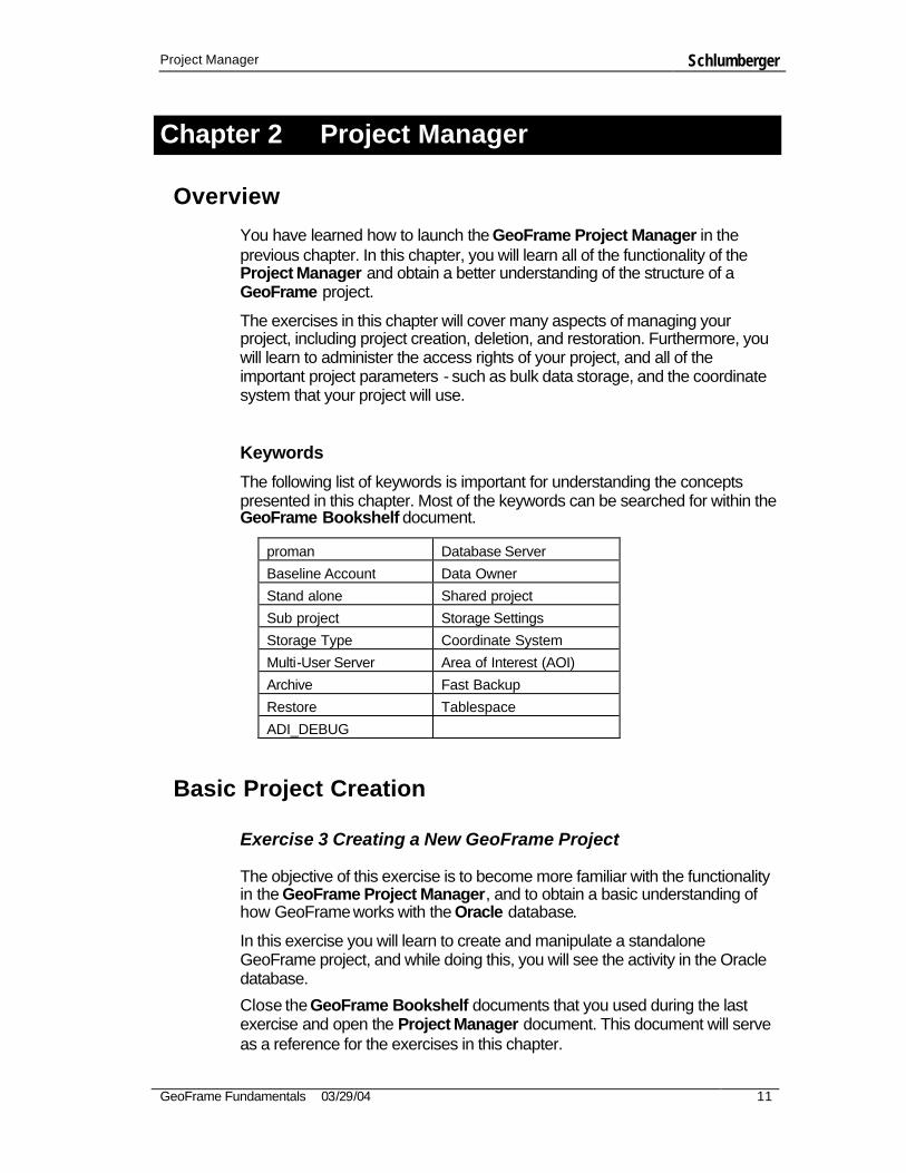
Keywords
The following list of keywords is important for understanding the concepts presented in this chapter. Most of the keywords can be searched for within the GeoFrame Bookshelf document.
proman Database Server
Baseline Account Data Owner
Stand alone Shared project
Sub project Storage Settings
Storage Type Coordinate System
Multi-User Server Area of Interest (AOI)
Archive Fast Backup
Restore Tablespace
ADI_DEBUG
Basic Project Creation
Exercise 3 Creating a New GeoFrame Project
The objective of this exercise is to become more familiar with the functionality in the GeoFrame Project Manager, and to obtain a basic understanding of how GeoFrame works with the Oracle database.
In this exercise you will learn to create and manipulate a standalone GeoFrame project, and while doing this, you will see the activity in the Oracle database.
Close the GeoFrame Bookshelf documents that you used during the last exercise and open the Project Manager document. This document will serve as a reference for the exercises in this chapter.

Project Manager Schlumberger
12 GeoFrame Fundamentals 10/06/03
In the previous exercise, you learned two different methods of launching the Project Manager. For this exercise you will launch the Project Manager from the command line again, however, you will set an environment variable that allows you to obtain additional debug information.
1. Open a GeoFrame Xterm from the Geonet window and set the environment variable ADI_DEBUG to equal 500.
prompt> setenv ADI_DEBUG 500 [return]
2. Launch the GeoFrame Project Manager by entering proman at the prompt. You should see a significant amount of information being displayed in the GeoFrame Xterm.
Note: The amount of information and the rate at which it is being displayed is somewhat useless unless you are troubleshooting a problem. The main objective of viewing the debug information at this point is to illustrate the amount of interaction with the Oracle database. The higher you set the ADI_DEBUG variable, the more information you receive from the console.
At this point you should have opened the GeoFrame Project Manager window.
Project Manager GUI - Login tab
Project Manager Schlumberger
GeoFrame Fundamentals 10/06/03 13
Questions:
• What is the name of the Database Server that you are connected to? Are there any other databases available to you? If so, try selecting one of them. Are there any projects available to you there?
When GeoFrame is launched, the default database (in the Database Server area) is queried for a list of projects that are owned by you or those which you have been granted access. Did you see the query happen in the GeoFrame Xterm when you launched GeoFrame ?
Look in the GeoFrame Xterm and locate the query for projects owned by you. What additional information was obtained for each project? (Hint: an SQL Query begins with the phrase: Select…)
DISCUSSION: How does GeoFrame find the Oracle database? What account was connected to that database? What is the significance of the catalog?
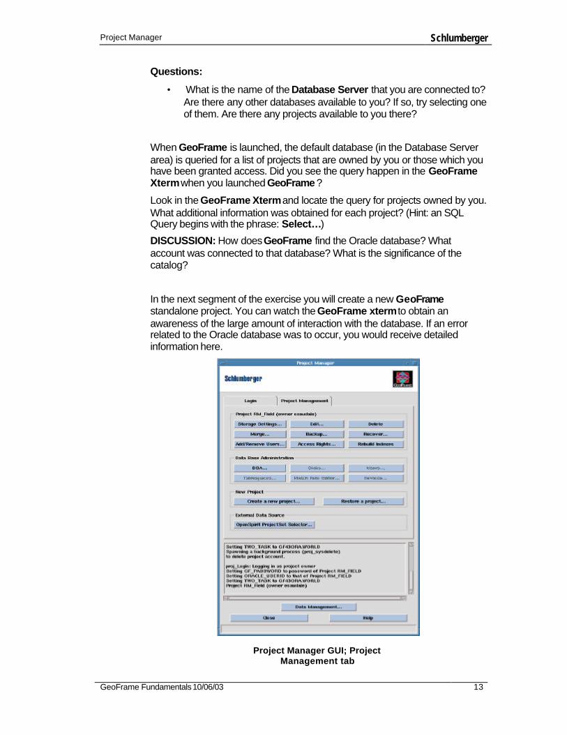
In the next segment of the exercise you will create a new GeoFrame standalone project. You can watch the GeoFrame xterm to obtain an awareness of the large amount of interaction with the database. If an error related to the Oracle database was to occur, you would receive detailed information here.
Project Manager GUI; Project
Management tab

Project Manager Schlumberger
14 GeoFrame Fundamentals 10/06/03
DISCUSSION: What options are available to you? Why so few? Discuss all of the buttons in the Project Management window. The Project Manager Help document contains information about all of the buttons in the Project Manager.
3. In the Project Manager window, click the Project Management tab.
4. Click the Create a new project button in the Project Management window.
Create a New Project Window
5. Enter a project name in the New Project Name field.
6. Enter a password in the Password field. For the scope of this course, you can use a password that is the same as the project name by double-clicking on the project name that you entered, and then middle- clicking (MB2) in the Password field. This will copy the project name into the Password field.
7. Verify the password by entering it again in the Password Verification field. (Click again with MB2 if you used the project name.)
8. Use the Default Tablespaces. Are there any others available to you? Why would there be additional Tablespaces for use?
9. Keep the Standalone project type and Medium Project Initial Size selected.
10. What Match Rule Systems are available to you? Choose the Default Match Rule System here.

Project Manager Schlumberger
GeoFrame Fundamentals 10/06/03 15
11. Click OK, and OK again, to proceed with the project creation. Watch the activity within the GeoFrame Xterm.
Each GeoFrame project has its own account in the Oracle Database. The first thing that happens upon creating a new project is the creation of this account. Oracle will not allow two accounts with the same name; therefore, you cannot have two projects with the same name within the same database.
12. When the Storage Settings window appears you can view the available storage locations that you have been granted permission to use for each Type of data to be stored. Select Default and Interpretation storage type.
13. Click OK in the Storage Settings window to proceed with the project creation.
14. When the Charisma window appears, select NO.
Project Parameters include many important variables. Refer to the GeoFrame Bookshelf document for a detailed explanation of these parameters. There are exercises later in the course material covering some of the items pertaining to Project Parameters, such as the Log Curve Preference System and the Well area of interest. This exercise will focus on the Coordinate System Settings.
15. In the Edit Project Parameters window, select Mean Sea Level for the Reference datum.
16. Click Multi-User Server Options. By default the multi-user server (commonly known as the PM Super Server) is going to start locally (on your machine).
17. In the Unit/Coordinate System area, click Set Units to set the unit system that you would like to use for the project.
18. Change the unit system to Metric. Click OK.
19. Click Set Projection to set the Geodetic datum for the project.
20. In the Set Projection System window, click Create to create a Coordinate System.
21. Click the button next to Projection and select U.S. State Plane Coordinate System.
22. Select Louisiana State Planes, Southern Zone, US Foot.
23. In the Create Coordinate System window click OK.
Note: By “Creating” a coordinate system you are not designing one, but choosing an industry recognized system and configuring it for use within your project.

Project Manager Schlumberger
16 GeoFrame Fundamentals 10/06/03
24. Select the Coordinate system you created in the Set Projection System window and click OK.
25. Click the Storage tab in the Unit/Coordinate System area and set the same coordinate system. You do not need to re-create it. It should be available for you to select.
DISCUSSION: Discuss the difference between the Display and Storage systems. Which can be changed at will? Which is recommended to remain consistent? What are the consequences of not specifying a coordinate system for the data?
26. Do not specify a Well Area of Interest at this time. Click OK to complete the project creation.
27. Click the Login tab in the Project Manager window. Do you see your new project? What is the catalog associated with it? When did you specify that?
28. Return to the Project Management tab. You should see all of the buttons available to you now (you are automatically connected to your project after creating it.) Using the Project Manager, you can change many of the parameters that you specified during creation.
29. Change the Display Unit system back to English. (Hint: start at Edit…)
30. In the Storage Settings window, remove one of the data storage disks from your project. Remove the disk specified by the instructor. Refer to the Bookshelf document for assistance if needed.
Add Project Users to GeoFrame Project
When a GeoFrame project is created, the project owner is the only project user. The project owner can then add some project users to work on the project. This is done in the Project Manager window. Project Management > Add/Remove Users…

Project Manager Schlumberger
GeoFrame Fundamentals 10/06/03 17
Add or Remove Users
The first step prior to adding access rights for a user, is to add the user to the project:.
31. Logon to an existing GeoFrame project that was prepared for you before the class. Ask your instructor about which project to logon to. This is a project owned by your Unix account, which contains data, and to which you will be able to grant access to other users.
32. After connecting, click the Project Management tab and then click the Add/Remove Users button to open the Add or Remove Users window.
33. Select your neighbor from the list of registered GeoFrame users that you can add to your project. Enter neighbor as a password for that user.
34. Click OK to close the Add or Remove Users window.
Project Manager Schlumberger
18 GeoFrame Fundamentals 10/06/03
Note 1: The neighbor that you add to your project should also add you to their project to make the exercise beneficial for both. For example, if you are user a1 and you add user a2 to your project, then user a2 should add user a1 to their project.
Note 2: When you select a password for an additional user, think about whether or not you want to use the same password as that of the Oracle project account. By using a different password for authorized users you can maintain an increased amount of security, as some of the scripts provided with GeoFrame require knowledge of the Oracle account password. This will also prevent users, whom you wish to have ‘read only’ privileges, from connecting directly to your project account using SQL*Plus, where they could update items or otherwise corrupt the project.
End of exercise 3
Access Rights Manager
Close the Project Manager Bookshelf document, if open. In the Bookshelf window, select Project > Access Rights Manager to open the Access Rights Manager User’s Guide.
In GeoFrame you can grant any level of access to a user. Upon adding them as a user to a project, they can automatically:
• Read all of the data in the project
• Update (change) all of the data in the project
• Delete all of the data in the project
• Create or load their own data
If you desire, you can deny privileges on data owned by other users:
• Update
• Delete
You can deny or grant privileges to data owned by specific users, and you can also create pseudo-users that own certain data, for which you would like to manage the access rights.
As part of administering the access rights to data owned by specific users, you can also change the ownership of data. Aside from the obvious use of changing data ownership, this can help allow groups of people to have access rights by implementing a pseudo-user that describes that group, i.e., data pertaining to Geologists should not be updated (or deleted) by Petrophysicists. Therefore a pseudo-user called “Geology” could be created, and the ownership of certain data could be transferred to the pseudo-user Geology. Now you can grant update and delete privileges to the necessary Unix users for all data owned by “Geology.” All of these tasks are accomplished by using the Access Rights Manager.

Project Manager Schlumberger
GeoFrame Fundamentals 10/06/03 19
Access Rights Manager
Exercise 4 Using the Access Rights Manager
Since access rights are granted to data owned by individual users separately, it is a good idea to see who currently owns the data in the project. In this example, use the project markers as the data type of interest. To determine the current ownership of the marker data in your project, use the Project Marker Data Manager.
1. Click the Application Manager from the Project Manager window.
2. In the Application Manager window, click Data.
3. In the Data Management catalog, open the Data Managers folder and start the Markers Data Manager.
4. In the Project Marker Data Management window, click Markers to open a Confirm window, asking if you really want to display a list of all of the Markers in the project. (You do.)
5. Click OK to display the list.
6. From the list, select all of the CARACAS markers, and click OK.
7. In the Project Marker Data Manager window, click Attributes to add the owner to the attributes that are displayed.
8. From the Available list in the Select Marker Attributes for Display window, click to highlight Owner and using the black arrow, move it to the Selected list. Click OK.
9. In the Project Marker Data Manager window, you can scroll to the right and see the new category Owner on the far right. The owner of the CARACAS marker data is traindev.

Project Manager Schlumberger
20 GeoFrame Fundamentals 10/06/03
The project owner, data owner, or the GeoFrame DBA can change the ownership of the data in the project. In the next steps, you will change the ownership of all of the Markers in the project to yourself, and the ownership of all of the Well Deviation Surveys to the neighbor that you added to this project. Imagine that the user you added earlier is the ‘group expert’ in managing and editing borehole deviation surveys. The expert should logically own the well deviation survey data and should have the ability to grant or deny access rights to edit or delete that data.
10. In the Project Marker Data Manager window, highlight the TVD value for the CARACAS marker in the Albite-F1 borehole.
11. Change the depth from 3150.1 to 3153.0. Click Apply.
Note: If the change was accepted, you have demonstrated your ability to alter the marker data in your project. Furthermore, you have demonstrated that in your project, you have the right to update data owned by traindev.
12. Return to the Project Manager window. Under the Project Management tab, open the Access Rights Manager and select Data Ownership.
Data Ownership window
13. In the Data Ownership window, select Marker for Display All Data of Type, to list all of the markers, and select you for the New Owner.
14. Click the Select all icon to highlight every marker.
15. Click Apply and OK in the Confirm window.

Project Manager Schlumberger
GeoFrame Fundamentals 10/06/03 21
16. You can observe that ownership has been transferred to you in the Data Ownership and the Project Marker Data Management window.
17. Close the Project Marker Data Management window.
18. Repeat the process of changing ownership of data and change the owner of all of the Well Deviation survey data to the neighbor that you added to your project previously. Verify the change in the Data Ownership window.
19. Click Cancel in the Data Ownership window to close it.
You have successfully added a user to your project, and changed the ownership of some of the project data. At this point, by default, the privileges are wide open for all of the data in the project for all of the users in the project. It is necessary to begin to restrict access to some of the data.
Note: In the Access Rights Manager window, the rows, labeled Project Users, listed on the left are all of the users that have been added to the project. The columns, labeled Users with Access Rights are the users who have assigned access rights to the data owned by them. The label on the columns could perhaps be correctly interpreted as “Data owned by”.
20. In the Access Rights Manager window, click Add/Remove Access Rights to add the names of the users whose data you want to restrict access.
Add/Remove Access Rights
21. In the Users with no Access Rights list on the left, select yourself as well as the new user that you added previously, and move them to the right side under Users with Access Rights by clicking on the Add arrow.
22. Click OK to close the Add/Remove Access Rights window.
23. In the Access Rights Manager window, observe that the update and delete privileges for your data and data owned by the new user can be restricted for all of the users listed on the left.
Project Manager Schlumberger
22 GeoFrame Fundamentals 10/06/03
Note: Remember that you transferred ownership of all of the Marker data to yourself, and the Deviation Survey data to the new user. That is the information you can control the access to now.
24. At the intersection of the row containing the new user and the column under your name (data owned by you), toggle the D to OFF, to prohibit the new user from deleting data owned by you in this project, but leave the U toggled to ON, to allow the new user to update your data in this project.
25. Restrict the access to ‘read only’ privileges on all of the data owned by the new user for everybody (except the new user). This will ensure that the new user (who is the expert on Well Deviation surveys) is the only person who can update (or delete) the Deviation Survey data.
26. Click OK to save all of these changes.
Test to ensure that these changes have taken been applied:
27. Start the Project Borehole Data Manager from the Data Management
Catalog.
28. In the Project Borehole Data Manager, click Boreholes to open a list of boreholes from which you can select for display. S
29. Select the Beryl-B4 borehole, and then click OK.
30. In the Project Borehole Data Manager window, click the Beryl- B4 borehole to highlight it.
31. Click the blue and white Information icon to open the Borehole Editor window.
32. Click Deviations and the Deviation Survey for the Beryl-B4 Borehole should already be highlighted.
33. Click Delete to delete the Deviation Survey from the project.
34. Click OK in the Confirm window. Were you able to delete it? Why not?
35. Click Details to verify the owner of the Deviation Survey data.
36. Cancel the details window and click OK.
37. Cancel the Select Preferred Well Deviation Survey window, the Borehole Editor window, and the Project Borehole Data Manager window.
To check the restriction of delete privileges on markers, you must log on to your neighbors project that added you as a user. In your neighbors project, attempt to delete a marker using the Marker Data Manager.
38. Close the Application Manager and return to the Login tab of the Project Manager window.

Project Manager Schlumberger
GeoFrame Fundamentals 10/06/03 23
39. Click Refresh Project List. You should see the addition of your neighbor’s project that you now have access to.
40. Connect to that project (the password is neighbor.)
41. Start the Marker Data Manager.
42. In the Markers Data Manager window, click Markers to open the Confirm window, asking if you want to list all of the markers in the project.
43. Click OK to display the list.
44. Select all of the CARACAS markers again, and click OK to display them.
45. Add the Owner attribute to the display again, but before clicking OK in the window to add the attribute, select the attribute within the Selected column and move it to the top of the list. You see the Owner at the beginning of the attributes.
46. In the Project Marker Data Manager window, find the CARACAS marker in the Albite-F1 borehole and highlight the entire row.
47. Click the red X icon to delete the marker. Could you delete it?
48. Select the TVD value for the CARACAS marker in the Albite- F1 borehole. Change the depth to 3150.1.
Note: You are able to perform the update because you have been given update privileges. You cannot delete the marker, but you may update it at your discretion.
49. Close the Project Marker Data Manager window and the Application Manager.
50. You should still be connected to your neighbor’s project in the Project Manager window. Open the Access Rights Manager and view the access rights that you have.
Note: You should see that the data owned by the project owner is all gray, because you have no ability to change the access rights on data that does not belong to you.
51. In the Access Rights Manager window, open the Data Ownership window.
52. Select to display all Well Marker data.
Note: Notice that the OK and Apply buttons are not even available for clicking in this situation. This is because you have no right to change the ownership of the markers in this project. The only data in this project that you are able to change the ownership of is data that is owned by you.

Project Manager Schlumberger
24 GeoFrame Fundamentals 10/06/03
53. Instead of displaying markers, select to display all data that is owned by you. Notice that the buttons are activated at the bottom of the window. You may transfer the ownership of data that is owned by you.
54. Close the Data Ownership window and the Access Rights Manager.
55. Return to the Project Manager Login window.
56. Close the Access Rights Manager Users Guide.
To this point you have utilized the GeoFrame Project Manager to create a stand alone project, manipulate some of the project settings, and managed the ownership and access rights of your project.
The next two exercises cover project backups and how to recover them. There are different types of backups available which will protect you against certain types of failures. Additionally, there are different issues regarding stand-alone projects versus Shared and Sub projects.
After completing the next exercise you should have a better understanding of the components of a GeoFrame project, and learn what needs to be captured in order to have a complete backup. Likewise, you will learn what needs to be removed in order to completely remove a project from the database and the GeoFrame environment.
End of exercise 4
Standalone Project Backup & Recover
In this section, you will create both Fast Backups and Archives of your GeoFrame project. For the purpose of this course, use the empty projects that you have created. This will result in faster backups, and will illustrate the procedures for backing up your project.
In the GeoFrame Bookshelf window, open the Project Manager Users Guide .
GeoFrame offers different methods of backing up your projects that account for both the Oracle segment of a project, and the data stored in the DSLs. The objective of this exercise is to introduce the methods of backing up projects and data that are available as part of the GeoFrame package, and to discuss what is happening in Oracle when using each of these backups. Furthermore, you will learn which types of backups are best for certain situations, for instance, moving a project versus having a backup for disaster recovery.

Project Manager Schlumberger
GeoFrame Fundamentals 10/06/03 25
Exercise 5 GeoFrame Project Backups
You should still be running GeoFrame from the GeoFrame xterm with the Debug variable set. You may find it interesting to watch the xterm as you perform the different types of backups in this exercise.
1. Connect to the standalone project that you created.
2. Click the Project Management tab and then select Backup…
Note: There are two types of backups available to you from the Project Manager, Archive and Fast Backup. There are differences in the amount and type of data that each will backup, as well as significant differences in what is required, in order to recover from each type of backup, depending on some of the options specified for each.
Project Manager Backup window
3. Toggle on Archive (in the upper right corner of the Backup a Project window) to create an Archive backup. Make the Destination Device a File . The default file location will be your user home directory, and the filename should default to something like this:
Archive_<project>_<date_&_time_stamp>.gfa
4. The default location and name will be fine. Click OK (in the Confirm window) to create the backup. Watch the activity the GeoFrame xterm.

Project Manager Schlumberger
26 GeoFrame Fundamentals 10/06/03
Note: Massive amounts of information pass by in the xterm, making the display quite useless until you have a problem. Once again, the main objective is to get an idea of the amount of activity, and to notice a difference between the Archive and the Fast Backup.
Create a Fast Backup of the same project. Select the Full Backup option. What do you anticipate the Full Backup will do? Make note the default name of the backup file for use later.
Note: The “slight” difference mentioned is only slight because there is no data loaded into your projects. Normally a relatively large amount of time and disk space would be required for the archive.
5. Create another Fast Backup but select Incremental Backup, and set the date to today’s date, if it isn’t already. What does Incremental Backup mean? Also make this backup to a file. Once again the default location and name will be fine. Note the .gfb suffix on the filename.
6. Watch the GeoFrame xterm. Aside from the slight difference in the length of time it took to perform the fast backup, what other event did you notice during the fast backup?
Note: This time there was almost no difference in the length of time between the two Fast Backups. This is due to the fact there is no data in the DSLs yet. Normally, if you had some data in the DSLs (300 to 400 Mb of Seismic data for instance), the Full Fast Backup would have taken additional time to include that data.
7. Click Cancel in the Project Backup window to return to the Project Management window.
You should have three backups of your standalone project at this point. We will delete the project from GeoFrame and try to restore the different types of backups.
8. In the Project Management window, click Delete to remove the project from GeoFrame.
9. Click OK to confirm the delete.
Note: It will take a while for Oracle to remove the account when you delete a project. If (in the next step) you get an error during creation of the project, the most likely reason is because the Oracle account hasn’t been dropped yet, and therefore the project name will exist.
10. Try to restore a project using the Archive Backup. Click Restore a Project from the Project Manager window and select the archive backup you created.

Project Manager Schlumberger
GeoFrame Fundamentals 10/06/03 27
11. Try to recover your project from the Full Fast Backup that you made. Click Recover from the Project Manager window and select the Full Fast Backup file you created. Then recover from the Incremental Fast Backup.
DISCUSSION: What condition should exist to be able to recover a project from incremental fast backup?
12. Map the DSLs for each storage type by selecting the desired storage type from the tabs in the Map Storage Disks window. You may increase the width of the window to see all of the storage types. Map the storage device on the left (which are those from the backup) to the available storage device on the right (which are those granted to you by the GF_DBA.)
13. Click OK to close the Map Storage Disks window when you are finished.
14. Click OK in the Project Recover window to proceed with the project recovery. After a successful recovery, click Cancel in the Project Recover window to close it.
End of Exercise 5
You have just learned how to make a backup of your project. The Incremental Fast Backup has the advantage of being fast and simple. It is a backup that can be performed easily every day, or as often as needed. It has the disadvantage; however, of not being a complete backup so that it must be recovered with the original project exist in the database. If the original project was deleted or corrupted, the project must be recovered from the Full Fast Backup prior to recovering from the Incremental Fast Backup.
A Full Fast Backup should be done prior to making an Incremental Fast Backup. A Full Fast Backup may be slower, but has the advantage of being able to be recovered anywhere, utilizing the Create a Project functionality. The GeoFrame Archive is also very complete and can be restored anywhere, however, there is no option to skip the bulk storage disks, making it a time consuming backup that is not suitable for everyday use.
Refer to the Project Manager Users Guide and the Guidelines for Project Clusters in the GeoFrame Bookshelf for additional reference on backing up standalone and Shared and Sub Project clusters.
Other Project Management Issues
You have just learned the difference between the different types of backups available to you within GeoFrame 4. In this exercise you will explore the
Project Manager Schlumberger
28 GeoFrame Fundamentals 10/06/03
remaining functionality in the Project Manager and learn how to review or change some of the project settings specified when you created the project.
This exercise is intended to make you aware of all of the settings and the locations of the settings for the project. Furthermore, it will increase your awareness of the implications of changing these settings during the life of the project. Much of the exercise should spark discussion based on the relevant Bookshelf documents, or the instructor’s presentation.
Exercise 6 Data Storage Settings
You may find it beneficial to perform this exercise while following along with the instructor.
1. Connect to your standalone project and move to the Project Management tab, to view all of the buttons available to you.
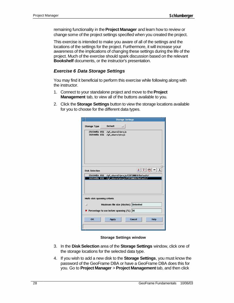
2. Click the Storage Settings button to view the storage locations available for you to choose for the different data types.
Storage Settings window
3. In the Disk Selection area of the Storage Settings window, click one of the storage locations for the selected data type.
4. If you wish to add a new disk to the Storage Settings, you must know the password of the GeoFrame DBA or have a GeoFrame DBA does this for you. Go to Project Manager > Project Management tab, and then click

Project Manager Schlumberger
GeoFrame Fundamentals 10/06/03 29
on DBA. Type in the GF DBA password (your instructor may tell you the password or he/she may demonstrate the following steps)
5. Click the Login tab, select a GeoFrame catalog then click Connect.
6. Go back to Project Management tab and then select Disks. This dialog is used to add disks for each storage type. Close this window.
7. Click Users and then select the newly added disks for each storage type.
8. Toggle on the user(s) that wish to have the new disks added then OK.
9. Click on User to go back to the regular user mode.
10. If you go back to the Storage Settings window, you will be able view the newly added disk(s) and can use them to store your data.
End of exercise 6
Log Curve Preference System
The Log Curve Preference System (LCPS) is a set of unique criteria, as determined by pre-defined or user-defined settings, used to search for log curves in the various GeoFrame applications. It is essentially a query tool and the queries are used to select log curves by Code or Name in the order defined in the Log Curve Preference System.
A number of pre-defined Log Curve Preference Systems have been developed for the user to select and use. Alternatively, the user can create a new system from one of the pre-defined systems, or from scratch, and modify it anyway as seen fit. For a new Project the "Use LCP System" option will be set to No and users need to change it to yes if the system is to be used, especially prior to working with Petrophysical applications such as ElanPlus and PetroViewPlus. The Data Functioning accessible from WellEdit and WellComposite can also take benefit of the LCP System.
Exercise 7 Using the Log Curve Preference System
1. Logon to an existing project if you have not already. In the Project Management tab, click Edit to open the Edit Project Parameters window.
2. Click on the Log Curve Preference System. The option Use LCP System should be set to NO. Leave it as is and close the LCPS window.
3. Close again the Edit Project Parameters window. Next, we will take a look at how what is in the LCP System. Detail information about LCP System is described in the LCPS Editor, which is accessible from Data Management catalog.

Project Manager Schlumberger
30 GeoFrame Fundamentals 10/06/03
4. Open the Application Manager, and then click on Data Management Catalog.
5. Open the Tools folder and then double click on Log Curve Preference System (LCPS) Editor.
6. In the LCPS Editor, select Demo One from the default Preference System.
7. Spend 5 minutes to explore how this Editor works. Later we will see how Data Functioning makes use of the system.
Log Curve Preference System from Edit Project Parameters
Edit Project Parameters window

Project Manager Schlumberger
GeoFrame Fundamentals 10/06/03 31
8. Open WellEdit from Application Manager.
9. Click Select Boreholes…and select Agate-H6, then click Run.
10. In WellEdit window, click to open the Data Functioning interface.
11. Type in RHOZ.OUT = RHOZ*1.2, highlight this syntax then click Evaluate . A window should come up with a message “Binding was not successful for RHOZ”. The reason for this is that Agate-H6 does not have density curve with code RHOZ. To make it work, we need to enable the LCP System.
12. Go back to the Data Management Tools > LCPS Editor, and select Demo One. Since we are not allowed to edit the default system, we will create a new one by copying from default. C
13. Click Create From…and select Demo One. Demo One_0 will be created.
14. Click to display the key values.
15. Under Select, change RHOB.CRC to RHOZ.
16. Under Code Key Values, add RHOZ in front of DEN. The row for Density should look like the following for Demo One_0
17. Click OK to save and close the LCPS Editor.
18. Go back to Edit Project Parameters and then set the Use of LCP System to Yes.
19. Select Demo One_0 as the one to use.
20. Go back to Data Functioning from WellEdit and repeat step 11. This time should work since the program searches for RHOZ and it will find RHOB instead as defined in the LCP System.
21. Close Data Functioning, WellEdit and LCPS Editor.
End of Exercise 7

Project Manager Schlumberger
32 GeoFrame Fundamentals 10/06/03
Multi-user Server Options
The multi-user server (or the super server as it is commonly called) is used to maintain data consistency among several applications sharing the same GeoFrame project. The first application that connects to the GeoFrame project will start this server. Other applications that connect to the project will pick up its address from the database. If not set to run persistently, the multi-user server will shut down when the last application exists a GeoFrame project.
Bulk Server Options
The bulk server is the mechanism by which bulk data is delivered to the application. The default setting for this is local to the machine GeoFrame is running. For small environment and those predominantly standalone projects, the default should provide acceptable performance. Selecting the remote host button will allow you to specify the host where bulk server will start.
Either the remote or local settings can be used in “Site mode”. This uses a common bulk server for each cluster project (Shared and Sub projects together).
For large sites, configuring bulk in this manner may be advantageous, much in the same way as using a separate Oracle server, as it allows the process to be run on a system that has the processing power to handle the task, and does not have the bulk competing with the application itself. The bulk service is installed on the server and is started (before GeoFrame is started) in order for the process to work.
Exercise 8 Multi-User Server Options
1. Click the Multi-User Server Options button in the Edit Project Parameters.
Multi -User Server Options window

Project Manager Schlumberger
GeoFrame Fundamentals 10/06/03 33
Question: Why would you want to run the Server on a different host?
Note: The different Multi-User Server Options are all useful. Your site-specific requirements may be the biggest factor in determining how the Multi -User Server is started (or found). Starting the server remotely may require additional remote shell capabilities, which may not be set up at your site. If it is intended for you to use a remote server, then your system administrator will make the appropriate system settings.
2. Cancel the Multi-User Server Options.
3. Click on the Bulk Server Options.
Question: What is the advantage of running Bulk Server on a remote host?
4. Cancel the Bulk Server Options window.
Unit/Coordinate System and Project Well Selection Options
5. In the Unit/Coordinate System area of the Edit Project Parameter box,
you will see the coordinate system you created and specified for your project. What are the implications of changing the Display coordinate system? What about the Storage coordinate system?
6. In the Project Well Selection Options segment of the Edit Project Parameters window you can choose to display only a segment of the wells in the project. Through a combination of Computing the well region, inputting corners, and Saving the AOI, you can create an Area of Interest that can be selected by clicking the Select AOI button.

Project Manager Schlumberger
34 GeoFrame Fundamentals 10/06/03
Note: You can create as many AOIs as you like, and change the AOI as often as you would like. Any time you wish to view all of the wells in the project you can select the Clear AOI button, so that no AOI will be applied to the project.
7. Click Cancel in the Edit Project Parameters window to close it.
Match and Merge Rules
What are match and merge rules?
The Match and Merge rules govern how incoming data is defined whether it is data loading using Data Load and ASCII Load or copying data through Data Copier in General Data Manager. Match and Merge rules apply in Standalone, Shared and Sub Projects.
• Match Rules define what attributes must be identical if the incoming data is to be considered duplicate.
• Merge Rules are instructions on what to do with duplicated or new data.
• Match Rules are defined and controlled at System level.
• Merge Rules are defined and controlled at Project level.
8. In the Project Management window, select Merge .
Merge Preference window
Project Manager Schlumberger
GeoFrame Fundamentals 10/06/03 35
Note: Later in the course you will learn to select and use a Merge Rule system. In the Merge Preference window, you can also choose to create your own Merge Rule templates (which will be available only to your project).Your instructor may demonstrate how you can view the Match rules, which requires to logon as a GeoFrame DBA.
9. In the Merge Preference window, click Select Template to view the site Merge Rule Templates available to you.
10. Click Cancel to close the Merge Preference window.
The final button in the Project Manager that has not yet been covered is the Rebuild Indexes button. Oracle uses indexes to improve the performance of the database by reducing the amount of time spent locating data (among other things). Over time, or due to considerable data changes, the indexes can become an inefficient collection of information that does not benefit Oracle the way it used to. Choosing to rebuild the indexes instructs Oracle to do that based on the current data in the DATA tablespace.
11. Rebuild the indexes in your project by clicking the Rebuild Indexes button. Select OK in the confirmation window when it asks you. Watch the GeoFrame xterm window to see this happening.
This marks the end of the Project Manager exercise. In the practical exercise scheduled for day two, you will have additional practice using some of the functionality of the Project Manager, including creating project clusters and working with Merge Templates.
End of Exercise 8


Process Manager Schlumberger
GeoFrame Fundamentals 03/29/04 37
Chapter 3 Process Manager
Overview
This chapter covers the Process Manager. After completing the exercises in this chapter, you will have a better understanding of the basic functions of the Process Manager and how the Process Manager can simplify all of your GeoFrame processing tasks. Furthermore, you will obtain a better understanding of the concept of Activities as it is used in GeoFrame . You will learn how to create activities, and learn the components that make up an activity.
Keywords
Knowledge of the following keywords will be beneficial to learning the concepts in this chapter:
• Activity
• Module
• Chain
• Data Focus
• Inspect
• Abort
• Halo Color
• Script
• Product Catalog
Modules, Chains, & Activities
In this exercise you will learn how to start the Process Manager and create a new activity, and then add modules and create chains. You should understand by the end of the exercise, how creating chains and saving them can make running repetitive tasks much more efficient.
Exercise 9 Process Manager
1. Close any Bookshelf documents you have open.
2. In the GeoFrame Bookshelf window, select Process to open the Process Manager Users Guide .

Process Manager Schlumberger
38 GeoFrame Fundamentals 10/06/03
3. In the Project Manager window, return to the Login screen and connect to the cloudspin project specified by your instructor. Once connected, start the Application Manager
4. In the Application Manager window, you can start the Process Manager by clicking on the Process icon.
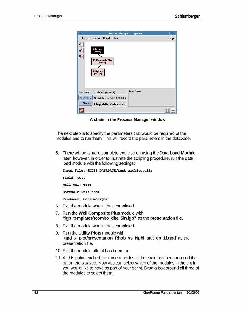
Process Manager window
You should see a fairly empty Process Manager window. When working with the Process Manager it will be helpful to you to understand some terminology:
• Module - A module is a GeoFrame program.
• Chain - A chain is a set of modules that are linked together.
• Data Focus - The data focus is the input data to be processed. We recommend that you always use borehole data items as your data focus.
• Activity - An activity is a group of one or more module chains and their associated data focus.
When working with Chains, it is important to realize that the output from one module in a chain becomes the input for the next module in the chain.
Create a simple activity by selecting and connecting modules:
5. Start a new activity by selecting File > New Activity from the menu.
6. Drag your cursor over the three icons in the upper left segment of the window and read what each of them does at the bottom of the window. Click the icon that allows you to Select a module from the Product Catalog.

Process Manager Schlumberger
GeoFrame Fundamentals 10/06/03 39
7. In the Product Catalog window, click Utility and select Loaders, Unloaders, and Converters.
8. Select Data Load and click OK.
9. From the Process Manager, you can start the module one of three ways:
• From the menu, select Edit > Start Module.
• By holding MB3 and selecting Inspect.
• By double-clicking the module.
Upon starting the module, the highlighting frame around the module turns green. At this point the module accesses the database to get the necessary arrays and parameters in order to run. For some modules, a slider bar will come up to indicate how the initialization process is running.
When the Data Load window appears, notice that the highlighting is yellow.
10. Click Exit to close the Data Load window, but do not delete the activity. Notice that the highlighting is brown, indicating that the Module has completed, and has exited properly.
In successfully selecting a module from the Product Catalog and running it, you have created an activity. Create a Chain by adding some more modules.
11. With the Data Load Module still highlighted, bring up the Product Catalog again.
12. Click ../go 1 level up and select Graphics from the Product Catalog and Well Composite Plus.
13. Click Apply.
14. From the Petrophysics catalog, select a Utility Plot module and click Apply.
Note: When a module is selected (black) and you select another module, a chain is automatically created. If you add a module without selecting or highlighting an existing module first, then the start of a new chain will be formed next to the existing one.
Since you may repeat these same steps for every well, you can save this module chain and reuse it. In saving this chain, you can actually create a new product group and add the chain to the Product Catalog.
Process Manager Schlumberger
40 GeoFrame Fundamentals 10/06/03
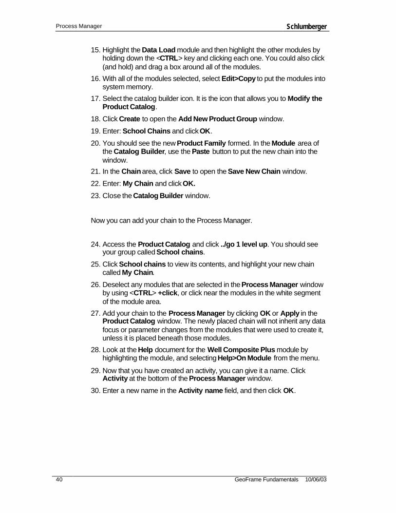
15. Highlight the Data Load module and then highlight the other modules by holding down the <CTRL> key and clicking each one. You could also click (and hold) and drag a box around all of the modules.
16. With all of the modules selected, select Edit>Copy to put the modules into system memory.
17. Select the catalog builder icon. It is the icon that allows you to Modify the Product Catalog.
18. Click Create to open the Add New Product Group window.
19. Enter: School Chains and click OK.
20. You should see the new Product Family formed. In the Module area of the Catalog Builder, use the Paste button to put the new chain into the window.
21. In the Chain area, click Save to open the Save New Chain window.
22. Enter: My Chain and click OK.
23. Close the Catalog Builder window.
Now you can add your chain to the Process Manager.
24. Access the Product Catalog and click ../go 1 level up. You should see your group called School chains.
25. Click School chains to view its contents, and highlight your new chain called My Chain.
26. Deselect any modules that are selected in the Process Manager window by using <CTRL> +click, or click near the modules in the white segment of the module area.
27. Add your chain to the Process Manager by clicking OK or Apply in the Product Catalog window. The newly placed chain will not inherit any data focus or parameter changes from the modules that were used to create it, unless it is placed beneath those modules.
28. Look at the Help document for the Well Composite Plus module by highlighting the module, and selecting Help>On Module from the menu.
29. Now that you have created an activity, you can give it a name. Click Activity at the bottom of the Process Manager window.
30. Enter a new name in the Activity name field, and then click OK.

Process Manager Schlumberger
GeoFrame Fundamentals 10/06/03 41
End of exercise 9
Note: GeoFrame gives each activity the same default name of Interpretation - <user_id>. It is very important to give all of your activities meaningful names, or you will quickly find that you lose track of which activity was used to interpret or process certain data.
You should have an understanding for how modules can be linked to form a chain, and how to save a chain for repetitive use (renaming each activity to keep track of the work you do!) The next exercise will allow you to become more familiar with the Script option in the Process Manager, which allows you to perform batch processing of data.
Scripting in the Process Manager
The Process Manager’s Script option allows you to run chains offline in batch mode. Batch processing is especially useful when you need to apply the same chain to a large data set, i.e., to a series of wells.
You can use scripts to construct module chains, set parameter values for modules, and execute commands. Note that when scripts are run, they examine the database and process data. They do not actually run the GeoFrame modules. You can create scripts that run interactively (prompting you for input) or non-interactively (in batch mode.)
Before you can run a script you must first create one. In order to create a script you need to create a module chain. The chain you created in the last exercise will work fine for the purposes of illustrating scripting.
Exercise 10 Generating a Script in Process Manager
1. In the Process Manager window, click File>New Activity from the menu to clear the existing chains.
2. Open the Product Catalog and select the chain you created in the last exercise.
3. Click OK in the Product Catalog window to bring your chain to the new activity.
4. Name the Activity in the Process Manager window: Script Generate.
Process Manager Schlumberger
42 GeoFrame Fundamentals 10/06/03
The next step is to specify the parameters that would be required of the modules and to run them. This will record the parameters in the database.
5. There will be a more complete exercise on using the Data Load Module later; however, in order to illustrate the scripting procedure, run the data load module with the following settings:
Input File: $DLIS_DATAPATH/test_archive.dlis
Field: test
Well UWI: test
Borehole UWI: test
Producer: Schlumberger
6. Exit the module when it has completed.
7. Run the Well Composite Plus module with “lgp_templates/tcombo_dite_5in.lgp” as the presentation file.
8. Exit the module when it has completed.
9. Run the Utility Plots module with “gpd_x_plot/presentation_Rhob_vs_Nphi_salt_cp_1f.gpd” as the presentation file.
10. Exit the module after it has been run.
11. At this point, each of the three modules in the chain has been run and the parameters saved. Now you can select which of the modules in the chain you would like to have as part of your script. Drag a box around all three of the modules to select them.
A chain in the Process Manager window

Process Manager Schlumberger
GeoFrame Fundamentals 10/06/03 43
12. In the Process Manager menu, select Script>Generate to open the Generate Script window.
Script Generating window
13. Select Help to view the reference document for Script building. This will allow you to quickly view the meaning of the six parameters in the box.
14. Give the script a name. The normal convention is an .scr suffix. Select the options as in the above figure: Query Bindings, Command Execution, and Comments.
15. Click OK to create the script.
Remember that the script was created with some parameters set from the module runs we did earlier. Prior to running your script, you may want to edit some parameters in it to make it more generic.
16. View your script by navigating to the directory in which it was created with your favorite text editor.
Note: The script we generated is not necessarily conducive to editing within the scope of this course; also it does not contain much information to edit. You can review the script editing guidelines in the Bookshelf document if you want to learn more about editing scripts.
17. To run your script, return to the Process Manager and create a new activity.
18. Click Script>Execute to run your script.
19. Click Script File to select the script file you created.
20. Select your script and click OK.

Process Manager Schlumberger
44 GeoFrame Fundamentals 10/06/03
Execute Script window
21. Leave the Arguments area blank. Since we did not select “Hard Code PM Focus/Container” when the script was generated, what do you expect to see?
22. Click Yes when it asks to continue and watch the Process Manager window.
When you generated the script from the modules that were just started and stopped, that is all that happened when you ran your script. The data load did not happen, because you chose no data focus at the start of the chain.
The Process Manager records all of your actions. Creating a script merely allows you to repeat the same steps over and over again, as is the case with any type of script.
Under normal circumstances in our scenario, you would have loaded some data and then processed the data in some way using the other two modules. If the desired processing would remain consistent and would be required for all of this type of data loaded into the project, then the only parameters would be for the Data Loading Module itself, as the data focus of the last two modules would automatically become the output of the Data Focus module. That is one reason not to hard-code the Data Focus.
You should have an understanding of how the scripting works, and perhaps can already imagine how it can make your job easier.
23. Close the Execute Script window and select File>Exit in the Process Manager window.
End of exercise 10
You should have an overview of how the Process Manager works and the information it records in the database. You should develop a habit of responsibly tracking your work by remembering to name your activities.

Process Manager Schlumberger
GeoFrame Fundamentals 10/06/03 45
The next chapter will introduce the GeoFrame Data Model and the General Data Manager.

General Data Manager Schlumberger
GeoFrame Fundamentals 03/29/04 47
Chapter 4 General Data Manager
Overview
The General Data Manager allows you to search for data, create, copy and delete data, and indicate specific data to be processed by other GeoFrame modules. Data is organized in GeoFrame in hierarchical groups called data items. The General Data Manager shows the data contained in your project in their hierarchical levels.
This chapter will cover two main topics, first the GeoFrame data model organization, then a description of the General Data Manager options.
After completing this chapter, you will have a better understanding of the GeoFrame Data Model and a description of the General Data Manager Options.
Keywords
The following keywords are useful and will assist you in understanding the topics presented in this chapter:
Data Model ID
Oracle Database Type
Bulk Database (DSLs) Source
Project Code
Field Name
Well Service Run
Borehole Tool Run
Container Arrays
GeoFrame Data Model
Data used in GeoFrame projects is stored in one of two places:
Parametric information about the data is stored in the ORACLE Database .
Additionally, some of the Bulk data previously (pre-GeoFrame 4.0) stored in the Bulk Database (or Data Storage Locations, DSLs), is now stored in the Oracle tablespaces. Bulk data files, such as seismic data, are stored in a directory tree in the Bulk Database. The GeoFrame Data Model provides access to the DSLs.

General Data Manager Schlumberger
48 GeoFrame Fundamentals 10/06/03
GeoFrame Data Storage
The GeoFrame data model is compliant with the Petrochemical Open Software Corporation (POSC) Epicentre standard.
GeoFrame data is physically stored in two separate repositories:
• ORACLE Database - contains all parametric information about data
• Bulk Database (DSLs) - stores bulk data files, such as log curves, images, multi-dimensioned arrays
Pointers to the bulk data are stored in the ORACLE Database.
The Data Model acts as a window into the Bulk Data. The General Data Manager (DM) manages all data and the Process Manager (PM) manages the interaction of data with various GeoFrame applications.
GeoFrame Data Model -> POSC Compliant
Bulk
PM/DM
Bulk Oracle Data
DataData
Applications
GeoFrame Data Model
GeoFrame Data Structure
Before you can use the General Data Manager, you should understand the organization of data structure in GeoFrame . Data is stored in GeoFrame as data items in a hierarchical order. At the top of the list is the project name.
One of the next major data items beneath the project level is the field data item. A GeoFrame project is composed of one or more fields.
Wells are stored next, under the field level, so that every well in GeoFrame is associated with some field.
Then boreholes are contained by wells. The borehole name and well name will be the same, unless the well contains one or more deviated boreholes. The diagram below shows the basic hierarchy of these major data items.
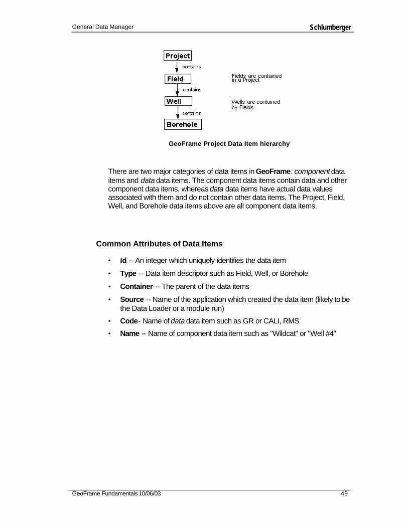
General Data Manager Schlumberger
GeoFrame Fundamentals 10/06/03 49
GeoFrame Project Data Item hierarchy
There are two major categories of data items in GeoFrame: component data items and data data items. The component data items contain data and other component data items, whereas data data items have actual data values associated with them and do not contain other data items. The Project, Field, Well, and Borehole data items above are all component data items.
Common Attributes of Data Items
• Id -- An integer which uniquely identifies the data item
• Type -- Data item descriptor such as Field, Well, or Borehole
• Container -- The parent of the data items
• Source -- Name of the application which created the data item (likely to be the Data Loader or a module run)
• Code- Name of data data item such as GR or CALI, RMS
• Name -- Name of component data item such as "Wildcat" or "Well #4"

General Data Manager Schlumberger
50 GeoFrame Fundamentals 10/06/03
Log Curve Data Type Hierarchy
Log curves are stored in the Project>Field>Well>Borehole data item hierarchy. The next major data item under the borehole data item is an activity. An activity is a group of service runs containing acquisition data or a Process Manager session, in which data was processed (for example, a data loading activity). The activity data item contains a data item called a service run, which is a group of tool runs containing acquisition data or the Process Manager group of modules in which data was processed. Service runs contain data items called tool runs. A tool run is data logged by a single tool in a service run, under the tool run is a data data item called an array. An array is a log curve.
If you load a DLIS file containing curve data, the activity, service run, tool run and array data items are created automatically. If you load other ASCII curve data, the tool run data item does not exist, but the activity and service run data items are created automatically as an ASCII load Process Manager session. The diagram below shows the major data items and structure of how log curves (arrays) are stored in GeoFrame.
Activity
Service_Run
Tool_Run
Arrays
BoreholeData itemhierarchyfromDLISfile:
Arrays
BoreholeData itemhierarchyfromASCIIfile:
Activity
Service_Run
Ex. Well #1
Loaded DataMay 06 10:30 1997
TOH .010(S320271)
SGTL(T320285)
GR.CALIBRATED.TOH.010 (a320565)
Ex. Well #2
ASCII_LoadApr 22 10:06 1997
ASCII_Load(S1088461)
SP.ASCII_Load(A1088529)
Log Curves
Log Curves
GeoFrame Log Curve Data Item hierarchy

General Data Manager Schlumberger
GeoFrame Fundamentals 10/06/03 51
Borehole Data Item Hierarchy
The diagram below is not intended to be comprehensive, but it will give you a more complete picture about the data structure in GeoFrame for the Borehole data item. Notice that Activity, Fault, Geoscience Interpretation, Horizon, and Lithologic Feature are other major data items under the Project level.
Project
Activity Fault FieldGeoscience
HorizonLithologic
Interpretation Feature
Well
Borehole Parameter Position
Activity Collection Coordinate Interpretation Parameter Position StratSystem Marker
BoreholeEquipment
Service Run
Parameter ParameterElevationReference
Array AxisIndex
AxisExtent Parameter
EquipmentItem Composition
ModuleRun
ToolRun
Binding
Array AxisIndex
AxisExtent
Parameter Tool String Equipment
Equipment ItemComposition
Equipment ItemConnection
Parameter WirelineTool
Array Collection Axis Index Zone SetCalibration EquipmentEquipment
Item CompositionParameter
Component Data Items
Data Data Items
GeoFrame Data Structure for Borehole Data Item

General Data Manager Schlumberger
52 GeoFrame Fundamentals 10/06/03
Data Type Definitions
There are hundreds of data types in GeoFrame . It is not in the scope of this training manual to discuss each of them, but the list below shows a number of the major data types and their definitions.
Data Type Definition
Activity The Process Manager session in which data was processed or a group of service runs containing acquisition data
Array A channel or trace; a log curve (Collection of indexed data values)
Borehole A borehole name associated with a particular well. The borehole name differs from the well name when the well contains sidetracks. (A unique oriented hole within a well.)
Collection A series of data items of any type
Coordinate_System A display projection set for a given geographic area
Core Sample taken at various depths in a borehole for study of the geologic and petrophysical properties
Cross_Section To display data (multi-wells) that is mutually correspondent in geologic position or laterally similar in character based on any property such as log curve, lithologic or fossil content or geologic age
Data_File Any file that contains data in ASCII or binary format
Dip_Set Data containing dip and azimuth values of formation beds, fractures or faults
Elevation_Reference Reference point of the log measurements
Fault_Marker A marker describing an intersection of a fault plane and a borehole
Feature_Boundary A naturally occurring feature or intersection of features found within or on the earth
Field The producing field name.
In exploration areas this name may be set to "Wildcat" or "Frontier" or "Unknown", etc. An administrative designation applied to a land area for the purpose of controlling oil and gas development.
Grid A model showing user-defined attributes such as depth, porosity, or contaminant concentration. It is often referred to as surface Grids consists of Z (attribute values) acquired at regular intervals of rows and columns of irregular X-Y locations.
Horizon A plane or surface separating two beds of rock in sequence or interface that indicates a particular stratigraphic sequence
Module_Run A specific instance of a GeoFrame application
Parameter A value that relates to a specific data item or string or number
Rock_Feature Also called layers, is a bed of rock indicating a particular

General Data Manager Schlumberger
GeoFrame Fundamentals 10/06/03 53
stratigraphic sequence
Seismic_Feature Seismic horizon
Service_Run The Process Manager group of modules in which data was processed or a group of tool runs containing acquisition data
Tool_Run Data logged by a single tool in a service run
Well A well name associated with a particular field
Well_Check_Shot_Survey Velocity surveys to perform well seismic calibration
Well_Deviation_Survey Data with measured depth, deviation angle and azimuth or dx and dy
Well_Marker A marker describing a point on a borehole that has not been promoted to a more specific type
Below are some other examples showing the Geoscience Interpretation, Activity, and Horizon data type structures.
Project
Activity Fault FieldGeoscience
HorizonLithologic
Interpretation Feature
AxisExtent
AxisIndex
Binset CoordinateSystem
CrossSection
CrossSectionPlane
Parameter Position SegmentSet
Parameter
Cross Section Hinge
Parameter
Parameter
AxisExtent
Geoscience Interpretation Data Type Structure

General Data Manager Schlumberger
54 GeoFrame Fundamentals 10/06/03
Parameter Service Run Data File
Module Run
Project
Activity Fault FieldGeoscience
HorizonLithologic
Interpretation Feature
Activity AxisIndex
BoundarySet
Grid Parameter
AxisExtent Parameter
Activity and Horizon Data Type Structures
Exercise 11 Using the General Data Manager
This exercise will introduce the General Data Manager, from launching it to displaying selected data in different ways, and to modifying or copying data.
By the virtue of its Oracle database structure, a listing of all log curves, for instance, in all boreholes is available quickly and easily in any GeoFrame project. Use the General Data Manager to organize and list these logs curves most efficiently.
1. Close any Bookshelf documents that you have open, and then view the Data Manager Users Guide. Locate the segment pertaining to the General Data Manager.
2. From the Application Manager, click the Data icon in the lower right corner to open the Data Management Catalog.
3. Open the Data Managers folder. The first manager in the list is the General Data Manager. Double-click the word General to open the General Data Manager. The window opens with the Project icon already highlighted.

General Data Manager Schlumberger
GeoFrame Fundamentals 10/06/03 55
The General Data Manager
4. With the Project icon highlighted, select MB3>Expand by Type>Field to produce a listing of the fields in the project.
5. Highlight the Amber field icon; select MB3>Expand by Type>Well to produce a listing of the wells in this field.
6. Highlight the Diamond-14 well icon. Slowly drag your cursor over the icons on the left side of the Project Manager window and read the description of what each does at the bottom.
7. Use MB3>Expand by Type>Borehole to produce a listing of the boreholes in this well.
8. With the Diamond-14 borehole highlighted, click MB3>List Log Curves to open the Log Curve List window.
9. Scroll through the list and highlight the following curves (use <CTRL> key for multiple selections): CALI, DPHI, DT, GR, ILD, SP, and TENS.
10. Open the Inter-task communication (ITC) door by clicking the door icon
in the lower right corner of the General Data Manager, in order to receive the selected log curves.
11. Click the Broadcast button in the lower right corner of the Log Curve List window to send the selected curves to the General Data Manager.

General Data Manager Schlumberger
56 GeoFrame Fundamentals 10/06/03
The seven curves will appear in the General Data Manager window and will be highlighted.
12. Click the Close button on the Log Curve List window.
13. Use the <CTRL> key to highlight only the GR and SP curves. Click the Playback icon (5th icon down on the left side tool bar) to graphically display these two log curves.
14. When finished examining these two curves, select File>Exit in the Playback window to close.
15. What is the TENS log curve? To find out, select File>Catalog Editor to open the GeoFrame Catalog Editor window. Ensure that the Select Catalog box is set to Array Catalog.
16. In the Find Catalog Entries box, set the toggle button to with Attribute, and make sure that Code is printed in the text entry field with the downward facing arrow. Then enter TENS in the white text entry box.
The Catalog Editor window
General Data Manager Schlumberger
GeoFrame Fundamentals 10/06/03 57
17. Click the Query & Add button. The unknown curve mnemonic is now identified as having to do with Cable Tension. For future reference, using the Catalog Editor in this way may identify any curve mnemonic you encounter, which is unknown to you.
18. Click Close in the GeoFrame Catalog Editor window.
End of exercise 11
You should have an understanding of the way the General Data Manager finds and displays data. You can also specify the information that you would like to see for each data item that is displayed.
Editing the Information Displayed in the General Data Manager
You may customize the way in which the display icons appear on the General Data Manager window. Often, it may be useful to have information on the create_date , the modified_by, the Sidetrack_number, etc., added into the display icon. Customization of the display icons is carried out as follows:
Exercise 12 Editing information in the General Data Manager
1. Click and drag a polygon surrounding the four well icons for the Amber field. After they are highlighted, click MB3 > Hide Children to clean up the display.
2. Highlight the Citrine-1 well; select Edit > Display Names to open the Display Name Format window.
3. Scroll down the list of entries in the Type box and highlight Well.
4. Click the blue Compose button to open the Compose Format window. The windows will overlap, so you should move one of them aside to view both.
5. In the Compose Format window, set the Add to format button to Attribute , then change the toggle button on the next lower level (which says create_date) to Name and click the Add button.
6. Change the toggle button (which now says Name) to ID and click the Add button.
7. Click Apply in the Compose Format window, and then click Apply in the Display Name Format window. The well icons in the General Data Manager now include the well name and the unique GeoFrame identification number for this data item (this well).
8. Back in the Compose Format window, change the Add to format toggle to read Characters.
General Data Manager Schlumberger
58 GeoFrame Fundamentals 10/06/03
9. In the text entry box, enter Phase1, and then click the Add button.
10. Click Apply in the Compose Format window, and then c lick Apply in the Display Name Format window. The well icons in the General Data Manager now include the well name, the unique ID number, and the descriptive term "Phase1".
11. Click Cancel on both the Compose Format window and the Display Name Format window to close them.
12. Highlight the Project icon, and then select MB3 > Hide Children to collapse the hierarchy back to the project level.
End of exercise 12
Generate Project Information ASCII File
Often it is useful to generate a file to output hard copy of information contained within the project. The General Data Manager helps to organize data and create such lists, which can then be sent to a printer to aid in project organization.
Exercise 13 Generating Project Information ASCII File
1. From the Project icon, select MB3>Expand by Type>Field to produce a listing of the fields in the project.
2. Highlight the Malachite field icon, select MB3>Expand by Type>Well to produce a listing of the wells in this field.
3. Highlight the Garnet-4 well icon, select MB3>Expand by Type>Borehole to produce a listing of the boreholes in this well.
4. With the Garnet-4 borehole icon highlighted, select MB3>Full Expand to create a listing of every data item in the hierarchy beneath the Garnet-4 borehole. This will take a few moments to complete.
5. After the expansion is complete, with all the expanded items highlighted, select File>Print List to open the Save Data Item Listing to File window.
6. Ensure that the Indented Listing toggle is on. In the text entry box under the Selected Filename heading, add the file name GARNET_WELL_LISTING to the file path (after the geoframe40x_sun directory), then click OK to close the window.
7. In a UNIX xterm window, cd to your geoframe40x_sun directory and find the file called GARNET_WELL_LISTING.
8. Enter: more and then the file name, to see a listing of the captured data hierarchy under the Garnet-4 borehole. With this ASCII File, you can
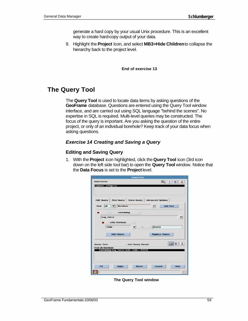
General Data Manager Schlumberger
GeoFrame Fundamentals 10/06/03 59
generate a hard copy by your usual Unix procedure. This is an excellent way to create hard-copy output of your data.
9. Highlight the Project Icon, and select MB3>Hide Children to collapse the hierarchy back to the project level.
End of exercise 13
The Query Tool
The Query Tool is used to locate data items by asking questions of the GeoFrame database. Questions are entered using the Query Tool window interface, and are carried out using SQL language "behind the scenes". No expertise in SQL is required. Multi-level queries may be constructed. The focus of the query is important. Are you asking the question of the entire project, or only of an individual borehole? Keep track of your data focus when asking questions.
Exercise 14 Creating and Saving a Query
Editing and Saving Query 1. With the Project icon highlighted, click the Query Tool icon (3rd icon
down on the left side tool bar) to open the Query Tool window. Notice that the Data Focus is set to the Project level.
The Query Tool window

General Data Manager Schlumberger
60 GeoFrame Fundamentals 10/06/03
2. Set up the query as follows: set the Find option to all.
3. Use the down arrow next to the word Activity, and select Borehole. Change the with Attribute toggle to containing, then click the down arrow and select the Log_Curve option.
4. Set the next toggle button down to read with Attribute , then use the down arrow to select the word " Code " and enter RHOB in the text entry box.
5. Click the blue Add Clause button, to add this query to the display box at the bottom of the Query Tool window. The text in this display window should read "Find all Borehole containing Log_Curve with Code = RHOB".
6. Click the Apply button to carry out the query. All boreholes containing a RHOB log will be highlighted in the General Data Manager window.
7. Save the query by clicking on the Save Query tab in Query Tool window.
8. Type in “boreholes with RHOB” in the Specify Query Name text entry then click on Save.
9. Click on the Edit Query tab and query for all boreholes containing RHOB or NPHI. The syntax should look like the following: “Find all Borehole containing Log_Curve with Code IN (RHOB, NPHI)”. Then save this query.
Hints: you can use comma (RHOB, NPHI) in the query.
10. Perform a query, but this time to look for all boreholes that contain both of RHOB and NPHI. The syntax should look like the following: “Find all Borehole containing Log_Curve with Code IN (RHOB) and containing Log_Curve with Code IN (NPHI)”. Then save this query.
11. How do you find 100 “most recent” log curves using the query tool?
• Hint: In the Query Tool, type in 100 after Find then select Log_Curve using the down pointing arrow.
Finding an Existing Query
The query tool allows you to reuse queries that have been predefined by the system or users. These predefined queries are stored in ASCII format. Each query file may contain multiple queries, each with a unique name. To reuse an existing query:
12. Open the Query Tool window (if you have closed it) and click on the Find Query tab. By default, it highlights the system_query.dat and lists all predefined queries by the system.
13. Select the query “Boreholes without Preferred Deviation Survey ” then Apply. As a result of this query, General Data Manager lists some boreholes that are identified as without deviation survey. Discuss with your instructor what it actually means.

General Data Manager Schlumberger
GeoFrame Fundamentals 10/06/03 61
14. Click on the user_queries.dat. This will allow you to reuse the queries you or other users have previously created. Cancel the Query Tool window.
Locating boreholes containing RHOB curves in Basemap
15. On your second screen, open a Basemap. From the GeoFrame Application Manager, click the Visualization icon to open the Visualization Catalog.
16. Double-click the word Basemap to open.
17. If this is the first time you have opened a Basemap in this project, you will be prompted to create a Basemap in the Select Model window when it opens. Leave the settings to Default, and click OK to view the basemap.
18. Post all the boreholes in your project (select Post>Borehole Sets).
19. Choose the Def_borehole_set and the def_traj_appear, and then click the large down arrow to move these selections into the lower window, and click OK to post the boreholes on the Basemap.
20. In the Basemap, select Send>Boreholes to enter the "send boreholes" mode, and then open the ITC door in the lower right corner of the window.
21. From the General Data Manager, broadcast the highlighted boreholes (those with RHOB curves) to the Basemap using the broadcast icon in the lower right corner. You know the distribution of boreholes in the project with density curves (they are highlighted in yellow).
22. In the General Data Manager window, with the boreholes containing RHOB logs still highlighted and the Query Tool still open on the screen, change the containing toggle to deeper than, and enter the value 12500 in the text entry box.
23. Click the blue Add Clause button and click Apply in the Query Tool window. Only the borehole Tourmaline has a RHOB curve and is deeper than 12500 feet. You may broadcast this to the Basemap to check the location of the Tourmaline borehole.
24. In the General Data Manager, highlight the Project Icon, then select MB3>Hide Children to collapse the hierarchy back to the project level.
25. In the Query Tool window, click Reset at the bottom.
26. Set up a new query as follows: set the Find option to all. Use the down arrow next to the word Activity, and select Grid.
27. Leave the with Attribute toggle as is, then click the down arrow and select the Name option.
28. Enter H* in the text entry box.
29. Click the blue Add Clause button to add this query to the display box at the bottom of the Query Tool window.

General Data Manager Schlumberger
62 GeoFrame Fundamentals 10/06/03
30. The text in this display window should read "Find all Grid with Name = H*", which means find all grids in the project with names beginning with the letter H. Click Apply to perform the query. Five grids should be found.
31. Double-click the grid called Houston_asap_twt_grid - Grid. A Grid Editor window will open. Notice that the Houston_asap_twt_grid is a two-way time grid of the Houston horizon, and ranges in value between 1437 ms and 1992 ms.
Note: Double-click any highlighted icon in the General Data Manager to obtain additional information about the highlighted data item.
32. Click Cancel to close the Grid Editor and the Query Tool window.
33. Highlight the Project icon, and then select MB3 > Hide Children to collapse the hierarchy back to the project level.
End of exercise 14
Collections
As the focus of work on a project changes, it is sometimes convenient to make collections of data items to facilitate work in the new areas. For example, if you wish to concentrate your interpretation efforts in the northeast corner of a 3D survey, you might create a collection of the wells in that area, or perhaps a collection of the GR curves from that area. A collection of wells is particularly useful in a project with 1000 or more wells; it can become tedious scrolling through lists looking for the wells you need. Making a collection simplifies this process. Collections can be made as follows.
Exercise 15 Creating a User Collection
1. If the Basemap you used earlier in these exercises is no longer open, open a Basemap again, and post the default borehole set as before.
2. Zoom in on the northeastern corner of the 3D seismic survey map where there are four boreholes posted (Citrine , Copper, Diamond and Calcite). We will make a collection of these boreholes.
3. In the General Data Manager, click the fourth icon from the bottom along the left side tool bar to open the User DataItem Collections window.
4. Click the Create button to open the Collection Editor window.
5. Open the door in the row of icons. Go to the Basemap, and click to select each of the four boreholes (make sure you are in Send>Boreholes mode). As each is selected, it appears in list form in the Collection Editor window.
General Data Manager Schlumberger
GeoFrame Fundamentals 10/06/03 63
6. In the Name field at the top, erase the name "New User_Collection”, and name this collection " east_boreholes ".
7. Click OK at the bottom to create the collection, and then click Cancel in the User DataItem Collections window to close that window. The collection has been created.
8. Make another collection. In the General Data Manager, highlight the Project icon, and then select MB3>Hide Children to collapse the hierarchy back to the project level.
9. Click the Query Tool icon (3rd down on left side tool bar) to open the Query Tool window.
10. Click the Reset button, then set up a query as follows: Find all Borehole, then move to the next lower level in the window and change the toggle button to read " penetrating Surface ", and enter the word Salt into the text box.
11. Click the Add Clause button to set the query, then click OK to carry out the query. A group of 11 boreholes, which penetrate the Salt surface, will be highlighted in the General Data Manager.
12. In the General Data Manager, click the fourth icon from the bottom along the left side tool bar to open the User DataItem Collections window.
13. Click the Create button to open the Collection Editor window.
14. In the Collection Editor window, open the ITC door in the row of icons.
15. Go to the bottom right corner of the General Data Manager and click the broadcast icon, to broadcast the selected boreholes into the Collection Editor window.
16. As before, erase the name " New User_Collection ", and enter your name followed by _Salt, (for example, " steve_Salt ").
17. Click OK at the bottom of the Collection Editor window to create the collection, and then click Cancel in the User DataItem Collections window. The second collection has been created.
18. Highlight the Project icon, and then select MB3>Hide Children to collapse the hierarchy back to the project level.
End of exercise 15
Data Copier
It is often required that individual data items (or collections of data items) be moved from one project to another. This is usually much easier than loading the required data into the second project using the available data loading tools. To move data between projects, use the Data Copier function as follows.

General Data Manager Schlumberger
64 GeoFrame Fundamentals 10/06/03
For someone to send items to your project, you must add them as a user to your project (with a password for access). For you to send data items to someone, they must add you as a user to their project (with password for access).
Exercise 16 Copying Data between GeoFrame Projects
1. To practice using the Data Copier Tool, pair off in the classroom and add each other as users. You will try to transfer the collection "your name_Salt" created in the previous exercise.
2. Both students in the pair must do this step so they can transfer collections back and forth. It is absolutely necessary to close the General Data Manager window, and then re-open it, so that GeoFrame will recognize newly added project users.
3. After adding each other to your projects, close the General Data Manager and then re-open it.
4. To send data, it must be selected (highlighted) in the General Data Manager. Use the Query Tool to find your collection.
5. Open the Query Tool; click Reset to reset the window. Set up a query to Find all, and use the down arrow to select Collection.
6. Change the toggle on the next line to read with Attribute .
7. Click the down arrow and scroll down the list to the last entry " more ".
8. Click more to open the Collection Attributes window, and scroll down the list alphabetically until you reach Name .
9. Click Name and then click OK to close the Collection Attributes window.
10. In the text entry box, enter *_Salt to force the query to find your collection by name (there are over 100 collections in the project).
11. Click Add Clause , and then click OK to carry out the query. The desired collection should be highlighted in the General Data Manager window.
12. Click the Data Copier icon (second from the bottom on the left side tool bar) to open the GeoFrame Data Copier window.
13. Highlight the project that you wish to send your collection to from the list near the top of the window (the project that your partner added you as a user) and enter the password that your partner has given you.
14. Set the Transfer Mode to File, and click the Export tab.
15. Leave the Merge Template set to Default.
16. Click the Export Data to selected Project button to send your collection to you partner's project
17. A series of information windows will appear as the transfer takes place, ending with a window that says “Data copy completed successfully”. Your partner can now find your collection in their project.

General Data Manager Schlumberger
GeoFrame Fundamentals 10/06/03 65
18. Close the Data Copier window and close the General Data Manager window to complete this series of exercises.
End of exercise 16
The exercises you have just completed have introduced much of the functionality of the General Data Manager. In the next exercise you can practice some more of the features and functionality available to you in the General Data Manger.
Later in the course you will have the opportunity to practice workflow using the General Data Manager after loading some data, which is covered in the next chapter.


Data Loading Schlumberger
GeoFrame Fundamentals 03/29/04 67
Chapter 5 Data Loading
Overview
This chapter covers loading data into your GeoFrame project using the Data Load module and the ASCII Load module.
The Data Load Module is used to load Digital Log Interchange Standard (DLIS) format data or Geoshare data into a GeoFrame Project. The module also loads LIS and other formats by first converting them to DLIS. You can use the data load module to load data from tape, disk, or a network device.
The ASCII Load Module is used to load a data that is in ASCII format. Well locations, deviation surveys, markers, log curves, checkshot surveys, descriptive data, core data, core image data, any image data in tiff format, scatter sets, and segment sets are all examples of data types that may be loaded with the ASCII Load module. As you will see, by creating your own control file, nearly any type of ASCII data could be loaded into a GeoFrame Project.
Keywords
The following list of keywords are important and will assist you in understanding the concepts introduced in this chapter.
Producer Alias DLIS Target Field
Western Atlas BIT Target Well LIS Target Borehole ACOUSTILOG Geoshare (RP66)
LA716 Control File
Data Load – DLIS Loading
The objective of this exercise is to introduce the Data Load module using a practical example of loading a DLIS file.
Exercise 17 Loading DLIS Files
1. Close any Bookshelf documents that you have open from the previous exercises, and open the Data Load Users Guide by selecting Data>Loaders and Savers>Data Load in the GeoFrame Bookshelf window.
2. Start the Data Load module located in the Data Management catalog.

Data Loading Schlumberger
68 GeoFrame Fundamentals 03/29/04
Data Load window
The following table helps describe some terminology and the functions of the buttons in the Data Load window. Refer to the Help document for further assistance.
Buttons and Fields Function
Input File Select data file(s) to load
Target Field Specify field name into which data is to be loaded
Target Well UWI Specify unique well identifier into which data is to be loaded
Target Borehole UWI Specify the borehole name into which data is to be loaded
Producer Specify the producer of the data
Alias Opens a sub-menu to select an alias file name that enables non-standard curves to be loaded
Library Filter Options Selects which arrays and objects to load
Preview Lists the logical files contained in the DLIS file you selected to load
Source Select File, Tape, or Network as the source of data to load
Unit/Coordinate Convert Converts the unit/coordinate of the loaded data item into the storage unit/coordinate of the project
Run Loads the file that you have specified
Exit Exits the Data Load module
Help Opens the online user guide

Data Loading Schlumberger
GeoFrame Fundamentals 03/29/04 69
3. To load a DLIS file, begin by specifying an input file. Check that the file option is selected, and click Input File from the Data Load main menu. This will open a window that will allow you to select files from disk.
4. Navigate to the directory specified by your instructor and select these three files:
sfe4_dite.dlis
sfe4_ldt_cnt.dlis
sfe4_msfl.dlis
Note: Data Load is used to load well data in the following formats: DLIS, LIS,
Western Atlas, BIT, ACOUSTILOG, LA716, Geoshare (RP66). If the data you are loading is in one of the above formats other than DLIS, the program converts the data automatically to DLIS format before loading it.
5. Click OK to select the files. Prior to loading the data, the Data Load
module allows you to preview the files that you would like to load in an ASCII format that is viewable by you. Select to view the contents of the sfe4_dite.dlis file .
6. Click the Preview button to see the logical files and data intervals.
7. Click View from the Data Load Preview menu.
8. Click sfe4_dite.dlis_dump listed under Files in the Select the Dump file to View menu.
9. Click OK. Scroll through the text editor. What is the well name and field name of the TOH.016 file?
10. Close the text editor by selecting File > Close.
11. In the Data Load Preview menu, select all files under Selected Files except TOH.016 and click the right arrow to remove the files from the list. (You may select multiple files by holding down the <CTRL> key.)
Note: At this point, you will have only loaded the TOH.016 file from the SFE4_dite.dlis file. All the others should be removed.
12. Click Next in the Data Load Preview menu to access a preview of the next DLIS file. It should read sfe4_ldt_cnt.dlis.
13. Remove all the files under Selected Files except TOH .034.
14. Click Next in the Data Load Preview menu to access a preview of sfe4_msfl.dlis.
15. Remove all the files under Selected Files except TOH.006 and TOH.008.

Data Loading Schlumberger
70 GeoFrame Fundamentals 03/29/04
16. Therefore, you would have selected TOH.034 file to load from the data file sfe4_ldt_cnt.dlis, and TOH .006, TOH.008 file to load from the data file sfe4_msfl.dlis and TOH.016 from sfe4_dite.dlis.
17. After selecting the files to load, click Close.
18. Click Target Field and enter Chimney Butte in the Selection box, and then click OK.
19. Click Target Well UWI and enter SFE #4 in the Selection box, and then click OK.
20. Click Target Borehole UWI and enter SFE #4 in the Selection box, and then click OK.
21. Click Producer and select Schlumberger.
22. Click Run in the Data Load menu. The message section will inform you when the loading is finished.
23. View the curves you just loaded in list form using the General Data Manager module of the Data Management Catalog in the Data Manager.
24. After opening the General Data Manager, highlight the project and expand by type to see if your new field was created. Locate the data you just loaded. (Will you perform a query? Or will you keep expanding?)
25. You can also check the loaded data in the Log Curves Data Manager. Click the Data Management catalog and highlight Log Curves then OK.
26. Prior to displaying log curves, select the following attributes in the order of: Code, Name, Borehole Name, Top Depth, Bottom Depth, Logging Direction, Maximum Value, Minimum Value and Catalog Description. To do this, click on the Attributes button and use the left/right arrows and up or bottom arrow, then close the Log Attributes for display window.
27. Click Boreholes under Table Setup and select the new borehole then OK.
You should leave the General Data Manager open, because we will check for the data you will load in the next exercises.
End of exercise 17

Data Loading Schlumberger
GeoFrame Fundamentals 03/29/04 71
Data Load – LIS Loading
You will be loading one of the accepted formats (LIS) so you should find this example to be remarkably similar to the last one; however, you will see how to utilize a log filter file to help specify the data you want to load. This time, you will be selecting a LIS file to load.
Exercise 18 Loading an LIS File
1. Click Input File in the Data Load window.
2. Select the directory as assigned by the instructor and click Filter.
3. Select the file rub_raw.lis to load. Click OK. Before moving on, create an array filter file, which will automatically select the log types that you specify when you run the loading process:
4. Make an array filter file containing the following curves:
DT SP DPHI GR LLD LLS NPHI CALI RHOB
Note: To do this, use vi (or any text editor you are familiar with) to create a file that contains the above curve names (one curve name per line, starting in column 1). Ask the instructor if you need help doing this.
5. Specify the array filter file you just created, so that only those curves will be loaded from the LIS file. Click Library Filter Options from the Data Load menu.

Data Loading Schlumberger
72 GeoFrame Fundamentals 03/29/04
6. Click Array Filter from the Data Load Library Filter Options menu.
7. Enter the full path name of the filter file (that you created) on the Select the Array Filter menu in the Selection text box.
8. Click Close.
9. Set the Target Field to Ruby.
10. Click Run to load the data.
11. View the curves that you just loaded in the General Data Manager. (Hint: select the new filed and choose to list all log curves.)
12. Or you can also view the log curves in the Log Curves Data Manager as you have previously done.
End of exercise 18
Note: It is possible to interactively filter the log curves that will be loaded as well. Select Library Filter Options in the data load window, and then specify Array in the Filter Customization section to accomplish this. You must also remove the reference to the filter file that you used previously.
Load Library Filter Options window
Data Loading Schlumberger
GeoFrame Fundamentals 03/29/04 73
You should have an idea of how to load DLIS and LIS files. Any of the supported formats work the same way in the Data Load module.
In the next exercise, you will learn how to load data using the ASCII Load module, which requires “informing” the module about the data. All of the formats that can be loaded using the Data Load module can also be loaded with the ASCII Load module; however, the ASCII Load module will allow you to load data in any format.
ASCII Load – Loading Well Locations
ASCII data is visible by you. It is usually a text file, divided into columns, not unlike a spreadsheet. Commonly there may be a few lines of header information specifying parameters that are common for every row or column of the data to follow. It is necessary to “inform” the module as to which columns contain what data. Using a control file does this.
There is little consistency in the ways contractors provide data, however with the ASCII Load module, and the ability to create a control file, you can be certain the right data values are read for a certain parameter.
The following exercise will combine ASCII load, merge and match rules exercises to show how users can modify the rules to change the default behavior.
Exercise 19 Loading Well Locations
1. Close the Data Load Bookshelf document and open the ASCII Load document. Refer to this document if necessary.
2. Start the ASCII Load module from the Data Management Catalog.

Data Loading Schlumberger
74 GeoFrame Fundamentals 03/29/04
ASCII Load Module
3. In the ASCII Load main window, click Input File(s) and select the assigned directory, and then select the /well_locations.dat file. Click OK.
4. Change the control file builder type from Log Data to Well Data (the option to the right of Create Control File) and click Create Control File button.
Note: The Control File Builder allows you to preview the data. The ASCII Loader uses the control file to locate the data within the file. A mistake in the control file can lead to the loading of erroneous data.
5. Under Data Preview, inspect briefly what the data looks like. Does the file have a header? This will determine if you need to specify the Start Row and Stop Row.
Note: Data Preview initially shows the first 100 lines of data from the first data file to assist you in creating a control file.
6. To enter Start Row, toggle on the button to the left of Start Row and then in the Data Preview section, click on the line that you want to be the first line processed by the ASCII Loader. You can leave the Stop Row and Record Length as is.
7. Select TAB for Column Delimiter and enter the Number of Columns.

Data Loading Schlumberger
GeoFrame Fundamentals 03/29/04 75
8. Under Database Information, select KB as the Elevation Ref. Code.
9. In the lower left corner of the Attribute Information window, ensure that Well data type is toggled on.
10. Toggle on the button next to Attribute Information, and then click Add Attributes.
11. Select Name , UWI, Location_X, Location_Y. Click OK.
12. On the lower left corner, change the data type from Well to Borehole; click Add Attributes then select Name , UWI, Bottom Depth, and Elevation Reference . Click OK.
13. In the Attribute Information section, specify the appropriate column number. Ensure that the format is set to String for the text strings and Float for data values containing decimals.
14. After you complete all information required for ASCII Loader to process your data, click OK to exit the Well Data Control File Builder.
15. In the ASCII Load window, click Target Field then type in EXP NORTH in the Selection text box and OK.
16. Click Run in the ASCII Load window to load the data.
DISCUSSION: What are the buttons for specifying the Input and storage coordinates used for?
How do you know if you need to use them?
If you did not specify anything, what was the coordinate system that was used for the data you just loaded?
17. View your new well data from the Project Borehole Data Manager. In the ASCII load window, toggle on Boreholes then click on Manager(s). The Wells and Boreholes data manager will open with the loaded data already displayed then click on Attributes…
18. Select PrefCS and PrefDS in the Selected list then move it to the Available list. Remove SpudDate from the Available list, then OK.
19. Do all of the boreholes that you have displayed have PrefCS and PrefDS set to Yes? What are PrefCS and PrefDS used for?
20. Do not close the Project Borehole Data Manager. We will use it later.
DISPLAYING THE WELLS IN BASEMAP
21. Open Basemap. Go to Application Manager > Visualization > Basemap then OK.
22. Click OK in Model Selector.

Data Loading Schlumberger
76 GeoFrame Fundamentals 03/29/04
23. Post all boreholes in Basemap. Go to Post > Borehole Sets.
24. Highlight Def_all_boreholes_set under Borehole Sets.
25. Highlight def_traj_appear under Borehole Appearances.
26. Click the down pointing arrow to move this selection then OK.
27. Zoom in the boreholes cluster on the upper right corner using . Define an area by MB1 press – drag then release.
28. After you view your well locations, iconize Basemap.
End of exercise 19
ASCII Load – Loading Well Deviation
You now have loaded the boreholes. Next we will load the deviation surveys using the data file that contains multiple deviation surveys.
Exercise 20 Loading Well Deviation Surveys
1. Open the ASCII Load module from the Data Management catalog, if you have closed it. If you still have it open, be sure to remove the previous input file before you select a new one.
2. Click Input File(s) and select the file all_deviations.dat in the assigned directory.
3. Change the button to the right of the Create Control File button, so that it shows Well Deviation Survey. Then click on Create Control File .
4. In the Well Deviation Survey – Control File Builder window, inspect the header of the input file. Complete the following information under the ASCII Format Information:
• What is the Start Row?
• Toggle OFF the Column Delimiter.
• Toggle ON the button next to Multi Borehole UWI then define its position and length from the Data Preview.
5. Under Deviation Survey Information section, click the Add Arrays button. Select MD, DX and DY in the Select Array window.
6. Define the Position and Length of the selected arrays from the data file.
7. Enter a new control file name: all_deviations.ctl next to the Control File button.
8. Click OK to close the Control File Builder window.

Data Loading Schlumberger
GeoFrame Fundamentals 03/29/04 77
9. In the ASCII Load main window, click the Target Field and select EXP NORTH.
10. Click RUN to load the deviation survey for all boreholes you loaded in the previous exercise.
11. Go back to the Project Borehole Data Manager that should have been open, highlight a borehole, and then click on the i-icon to bring up the Borehole Editor window.
12. In Borehole Editor, click on Deviations, highlight the newly loaded deviation survey, and then click the i-icon to open the Deviation Survey Editor.
13. Briefly quality control by comparing the loaded deviation survey for this borehole with the data file. Does it look like that data being loaded correctly? If the loaded data looks correct, then proceed to the next step. If it looks wrong, go back to the ASCII Load module and discuss with your instructor to try finding out what parameters that were set incorrectly, make the corrections and re-load again.
14. Click Set Preferred. The program may complain that some arrays are missing. Click OK on the information message. We will then compute the missing arrays.
15. Click Compute and under Computation select TVD/TVDSS/DEVI/AZIM in Compute window then OK. The missing arrays will be computed.
16. Click Set Preferred again. This will set the new deviation survey as preferred for this borehole. You can check this in the Project Borehole Data Manager.
17. Click to view the deviation data in a 2D graph. Spend some times to inspect how this tool works. This is a basic quality control tool that allows you to visually inspect the data for integrity and accuracy.
18. When you are finished, click Cancel to close the tool. Then Cancel the Deviation Survey Editor to close it.
19. Click OK to close the Select Preferred Well Deviation Survey window then close the Borehole Editor.
You have just computed missing arrays for only one borehole. You will have to compute all missing arrays for the rest of the boreholes in order to set the deviation surveys as preferred. Instead of computing the missing arrays from the Borehole Editor for each of the borehole, Project Borehole Data Manager provides an option to compute and set them as preferred in one go.
The next steps will show you how to do just that:
20. Highlight all boreholes contained by EXP NORTH Field.
21. On the lower right of Project Boreholes Data Manager, click Compute Surveys. This will bring up the Compute Surveys window.
22. Ensure that the Set Preferred and Skip Boreholes with Preferred Surveys are toggled ON.

Data Loading Schlumberger
78 GeoFrame Fundamentals 03/29/04
23. Click Preferences and move Last created survey from left to right. This particular step is to make sure that the last created survey will be set as preferred (it is necessary for the students who loaded the data more than one time).
24. Click Deviations tab.
25. Next to the Compute option, select TVD/TVDSS/DEVI/AZIM.
26. Click Apply and then check in Project Borehole Data Manager that the boreholes have the PrefDS set to Yes.
27. Close the Compute Surveys window by clicking Cancel. Keep Project Borehole Data Manager open. We will still use it in the later exercise.
28. In Basemap, view these updated wells. You should have your Basemap already open.
End of exercise 20
ASCII Load - Loading Well Checkshot Surveys
The following exercise will give you the opportunity to load Well Checkshot surveys to the same set of boreholes.
Exercise 21 Loading Well Checkshot Surveys
Go back the ASCII Load module or open one if you have closed it. If you are not using the new run of ASCII Load module, be sure that you remove the previous input file before you select a new one.
1. The input file to load the checkshot surveys is all_checkshots.dat. Change the Create Control File option to Well Checkshot Survey.
2. Click Create Control File button and briefly inspect the file and then complete the parameters under ASCII Format information:
• What is the Start Row for this file?
• What is the Number of Column in this file?
• What type of Column Delimiter does the data file have?
• Toggle ON the Multi Borehole UWI and specify its column.
3. Get the information from the data file under Data Preview to complete the parameters under the Checkshot Information section.
Hints: The Checkshot Elevation Reference (ER) is KB; The Elevation at Time Zero (ETZ) is Mean Sea Level (MSL).

Data Loading Schlumberger
GeoFrame Fundamentals 03/29/04 79
4. Click Add Arrays then select TVD and TWOTIM.
5. Specify the column for the TVD and TWOTIM, then OK.
6. Click Run.
After the load is complete, go back to the Project Borehole Data Manager. You should still have it open but if you have closed it, reopen it from Application Manager > Data > Data Managers > Wells and Boreholes.
7. Display all boreholes contained by EXP NORTH field then highlight any borehole. Click the i-icon to open the Borehole Editor.
8. Click Checkshots in Borehole Editor. Ensure that your newly loaded checkshot is highlighted then click the i-icon. This will open the Well Checkshot Survey Editor.
9. Take a few moments to inspect and QC the data. You can also utilize the
2D graphic tool by clicking on . When you are finished, close the 2D graph, Well Checkshot Survey Editor and Borehole Editor.
All checkshot surveys that you loaded contain TVD and TWOTIM arrays only, it is sometimes convenient to have additional information of MD array. The best way to compute automatically the MD array for multiple boreholes is through the Project Borehole Data Manager.
10. In Project Borehole Data Manager, highlight all boreholes then click on Compute next to Surveys to open the Compute Surveys window.
11. Toggle OFF Set Proffered and Skip Boreholes with Preferred Surveys.
12. Ensure that the Checkshots tab is selected, then choose MD next to Compute option.
13. Click OK. This will compute the MD array then close the Compute Surveys window. If you wish to view the result, you need to open the Borehole Editor for a borehole then click Checkshots from the Borehole Editor window.
End of exercise 21
ASCII Load – Loading Well Markers
In the next exercise, you will learn how to load Well Markers for the same set of boreholes.

Data Loading Schlumberger
80 GeoFrame Fundamentals 03/29/04
Exercise 22 Loading Well Markers
If you are using the same ASCII Load window, be sure that you remove the previous Input File(s) before you select the new one.
1. Select the input file to load Well Markers, which is well_markers.dat file from the assigned directory.
2. In the ASCII Load window, change the button to the right of the Create Control File button, so that it shows Well Marker Data and then click Create Control File .
3. Ensure you set a correct Start Row, Column Delimiter and Number of Columns in the ASCII Format Information section.
4. In the Database Information, ensure that Well Marker Type is set to Strat_Marker. Leave the other parameters as is.
5. Click Add Attributes in Marker Information section. Select Borehole_Name , Borehole_UWI, Name , Depth/Time , and Well_Marker_Type then click OK.
6. Specify the columns for each attribute.
7. Next to the Control File button, type in a new name for this marker control file in the text entry box. Then OK to save the marker control file.
8. In ASCII Load module, click Run to load the data.
9. When loading is complete, toggle on Markers in ASCII load window, then click on Manager(s). The Project Marker Data Manager will open with markers already displayed. QC the loaded markers to validate if they look correct. If they do not look correct, you must check if some parameters were not set properly in the control file.
10. Do not close the Project Marker Data Manager.
Loading new markers into GeoFrame will create new surfaces with the same names, if they do not exist already and associate them automatically. The next exercise will give you the opportunity to look at these new surfaces, which were created from loading the markers.
As you have noticed, the loaded markers do not have the colors set appropriately since that information was not provided in the data file. Editing all markers in Project Marker Data Manager is very time consuming and impractical if you deal with hundreds or thousands of markers. A more practical way to edit the marker attributes (color and/or name) is by editing the surfaces in the Project Surface Data Manager then using the Update Markers (Color and/or Name) option.
11. Open Project Surface Data Manager from the Application Manager. Data Management catalog > Data Managers > Surfaces.
12. Under the Table Setup, click Filter.., and then ensure that only Gal_Loader is toggled ON.

Data Loading Schlumberger
GeoFrame Fundamentals 03/29/04 81
Note: The reason for doing this is that we only wish to display the surfaces created by GAL Loader (ASCII Load module) and avoid displaying all surfaces in the project. Any data item created from the ASCII Load module will have Gal_Loader set in the source attribute.
13. You should get 9 new surfaces with no colors assigned. Edit the colors for each surface by double clicking on each color cell to open the Color Selector then select the color you wish to assign.
14. After you complete editing the colors for each surface, click Apply to save the changes to the database.
15. Highlight all surfaces. Under Operations > Update Markers, change Both to Color. Then click Update Markers. Click OK in the confirmation message that pops up.
16. Now, go back to the Project Marker Data Manager and validate if all markers have the colors changed according to the colors from the surfaces.
17. Close both Project Marker and Project Surface Data Managers.
18. Let’s post the well markers in Basemap. In Basemap, go to Post > Interpretations.
19. Click on Markers and select Trim_B3 from the Content tab.
20. Click on Appearance tab and change color from Surface Color to User color then pick any color other than red.
21. Change the Index to MD.
22. Under Marker Labels, select bigger size than default.
23. Under Label Type and Placement, highlight then drag and drop Marker Name into the placement box. Click OK to close Post Markers window. Then close the Interpretation window.
Gridding Well Markers in Basemap
24. Grid the markers in Basemap. Go to Gridding > Project Gridding.
25. Click on Use Posted Data then OK.
26. Save the grid and contour. Go to Gridding > Save As. Change the name of Grid and Contour from Time to a more meaningful name.
27. Check if this grid is already saved in the database. Open the Grid Data Manager and Grid Library Data Manager. Go to Tools > GF Applications.
28. Take sometimes to explore and discuss these data managers.
End of exercise 22

Data Loading Schlumberger
82 GeoFrame Fundamentals 03/29/04
ASCII Load - Loading Multiple LAS Files
Your GeoFrame project should now contain some well data that was loaded previously, such as deviation surveys, checkshot surveys and well markers, with the exception of well log curves, which we will load for the same set of borehole in the following exercise. The log curve data are in the LAS format.
Loading log curves in LAS format in GeoFrame ASCII Load is very straightforward. In general, LAS data contains a log curve header including name of the field, UWI, Well X and Y positions, etc. You are going to load the logs into the wells that already have the X and Y positions. The LAS data may contain the X and Y positions that are different from those in the project. To avoid updating the existing X and Y positions with the new ones from the LAS files, we have to modify the merge rules prior to loading.
Exercise 23 Loading LAS Files with Modified Merge Rules
1. Go to the Application Manager, click Data to open Data Management catalog.
2. Open the Tools folder and select Merge Preference Setting Tool then OK.
3. Click Template Editor to open the Merge Rule Template Editor
4. Select File > Save As to save a copy of the Default Merge Rule Template as User_Skip_LAS_Position.
5. Click Add Data Type to open Add Type, which list available data types.
6. Select Position and OK. For Position, changed the Merge Operations toggle to Skip/Ignore. This will tell the program to skip on updating the position of the wells.
7. Exit from Merge Rule Template Editor, File > Exit.
Go back to the ASCII Load window, or open a new one if you have closed it. Ensure that previous input files are removed, and then select the following LAS files from the directory indicated by your instructor:
OCSG_1172_A1.LAS 17706402860000.LAS
OCSG_5196_1.LAS 17706402960000.LAS
1770640387000.LAS OCSG_1172_A7.LAS
1770640264000.LAS
8. In ASCII Load module, click Merge Template and select the user defined merge template.

Data Loading Schlumberger
GeoFrame Fundamentals 03/29/04 83
9. Use the down pointing triangle to select las_depth from the predefined Control File as shown in this graphic.
10. Click Producer… and select SLB, then RUN.
11. Take some times to inspect the newly loaded logs, toggle on Logs then click Manager(s).
12. Close the Project Log Curves Data Manager.
End of exercise 23
Computing Litho Zones from Surfaces/Markers
Litho Zones in GeoFrame are defined as a set of lithology intervals or zones that intersect with borehole trajectory. Several different applications and data managers can be used to access and create litho zones, for example, WellPix, Project Litho Zone Data Manager, Project Borehole Data Manager, Geology Office Composite and Cross Section.
The following exercise will introduce you to computing and accessing litho zones for the boreholes contained by EXP NORTH from the Project Borehole Data Manager and Project Litho Zone Data Manager. Creating litho zones from geological applications such as WellPix, Geology Office Composite and Cross Section are introduced in the two-day Geology Office course.
This exercise is necessary prior to loading production data in the next exercise.
Exercise 24 Computing LithoZones from Project Borehole Data Manager
In Project Borehole Data Manager (open one if you have closed it), ensure that you display all boreholes contained by EXP NORTH Field.
1. Change the Compute Surveys to Compute Litho Zones, and then click the Compute button. This will open Compute Litho Zones window.
2. Click Boreholes… and ensure that all boreholes contained by EXP NORTH field are highlighted.
3. Click Preferred Owner and select yourself as the owner (whatever your user name is).
Data Loading Schlumberger
84 GeoFrame Fundamentals 03/29/04
4. Click Surfaces… and highlight all horizons. Deselect the fault if any.
5. Click Create Zone Version…then type in Computed_zones next to Name, then OK.
6. Under Options, ensure that the following options are toggled ON:
• Last Modified Marker
• Create New Litho Zones If Non-Overlapping
• Use Top Surface Color
• Generate Layers
• Open Zone Data Manager After Creation
7. Click Create Litho Zones. Wait for a while and Project Litho Zone Data Manager will pop up with the new litho zones displayed.
8. Cancel the Compute Litho Zones window.
9. Take some times to inspect the litho zones in the Project Litho Zone Data Manager.
You will notice that each litho zone is associated with a layer and all Litho Facies are set to Undefined. Let’s assign a litho facies for each litho zone. You can definitely edit the Undefined to a litho facies in Project Litho Zone Data Manager but this will be cumbersome if you deal with hundreds or thousands of litho zones. A much better way to edit the Undefined to a litho facies is from the Project Layer Data Manager.
10. Keep the Project Litho Zone Data Manager open. Bring up the Project Layer Data Manager (Application Manager > Data > Data Managers > Layers).
11. In Project Layer Data Manager, click Zone Version and select the zone version that contains the litho zones you wish to display.
12. Scroll to the right to get to the Litho Facies column. Double click on each Litho Facies cell and assign a litho facies.
13. After you complete editing the litho facies, click Apply and then highlight all litho facies.
14. On the lower right and next to Update Zones, select Litho Type.
15. Click the Update Zones button and OK in the confirmation window.
This operation changes the litho facies in the Project Litho Zone Data Manager.
16. Now, go back to Project Litho Zone Data Manager and you should notice that each litho zone has now been assigned to a litho facies.
17. Display the litho zones in Basemap. Go to Basemap, Post > Interpretation.
Data Loading Schlumberger
GeoFrame Fundamentals 03/29/04 85
18. Click Zone Intervals, then select the zone version you created previously from Select Zone Version….
19. Highlight all layers using the select all icon then OK. Close the Interpretation window.
20. Briefly view the litho zones displayed in Basemap then iconize Basemap.
ASCII Load - Loading Production Data
This exercise is another example of the type of data that can be loaded using the ASCII Load module. As you progress through these exercises, you will notice the different parameters that are important for each data type.
Exercise 25 Loading Completed Intervals Data
Go back to the ASCII Load module; open one if you have closed it. Ensure that the previous input files were removed. We will select a new input file, which is completed_interval.dat
1. Change the control file to Completed Interval Data, and then click the Create Control File button.
2. Inspect brief the data file under Data Preview then specify the parameters under ASCII Format Information.
• What are the Start Row, Number of Columns and Column Delimiter?
• Toggle ON the Multi Borehole UWI and type in the column for the UWI.
3. Type in completed_interval.ctl next to the Control File button.
4. Click the Add Attributes button under the Interval Information section, and then select the following attributes:
• Top Depth, Bottom Depth, LayerName, Name, Oil Flowrate and Water Flowrate.
5. Specify the column for each attribute then OK.
6. Click RUN.
7. When the Load is complete, toggle on Completed Intervals, then click Manager(s) to open the Completed Intervals Data Manager. Inspect the newly loaded completed interval data.
8. Close ASCII Load and Completed Intervals Data Manager.
You should have an understanding of how the different Data Loaders work, and the scope of the data that can be loaded with them.

Data Loading Schlumberger
86 GeoFrame Fundamentals 03/29/04
Posting Completed Intervals In Basemap
9. Go to Post > Production data. Change the Post Data Type to Completed Interval Production.
10. Select the layer H250_Trim_A.
11. Drag and drop Oil Flowrate and Water Flowrate from the Available Properties to Selected Properties.
12. Click OK to post the production data.
13. Double click on a borehole in Basemap. It will open the Borehole Editor for that borehole. QUESTION: From the Borehole Editor, can you find out quickly what data is contained by this borehole?
14. Take some times to explore how you can access project data managers from Borehole Editor to obtain quickly the data contained in the borehole. Click on the Markers, Zones (with different selections) or Log Curves buttons.
End of exercise 25
How to manually enter well data into GeoFrame Project Data Managers
GeoFrame allows you to manually enter data in most of Project Data Managers. The following provides you with a hands-on exercise on how to create a well location, well deviation and well checkshot survey manually.
Exercise 26 Manual Entry of Well Data
1. Open Project Borehole Data Manager if you have closed it.
2. Display all boreholes contained by EXP NORTH Field.
3. Click on Add then OK to add empty line below current row.
4. Type in a borehole name and UWI.
• Type surface location X = 1700400 (ft); Y = -143000 (ft).
• KB = 95 ft
• Bottom Depth 6000 ft
• Then Apply.
5. Highlight the new borehole then click on the i-icon to open the Borehole Editor.
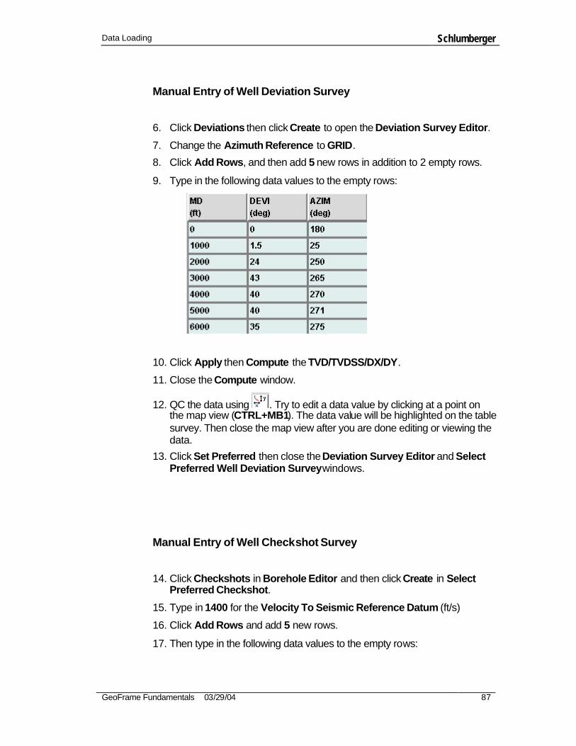
Data Loading Schlumberger
GeoFrame Fundamentals 03/29/04 87
Manual Entry of Well Deviation Survey
6. Click Deviations then click Create to open the Deviation Survey Editor.
7. Change the Azimuth Reference to GRID.
8. Click Add Rows, and then add 5 new rows in addition to 2 empty rows.
9. Type in the following data values to the empty rows:
10. Click Apply then Compute the TVD/TVDSS/DX/DY.
11. Close the Compute window.
12. QC the data using . Try to edit a data value by clicking at a point on the map view (CTRL+MB1). The data value will be highlighted on the table survey. Then close the map view after you are done editing or viewing the data.
13. Click Set Preferred then close the Deviation Survey Editor and Select Preferred Well Deviation Survey windows.
Manual Entry of Well Checkshot Survey
14. Click Checkshots in Borehole Editor and then click Create in Select Preferred Checkshot.
15. Type in 1400 for the Velocity To Seismic Reference Datum (ft/s)
16. Click Add Rows and add 5 new rows.
17. Then type in the following data values to the empty rows:
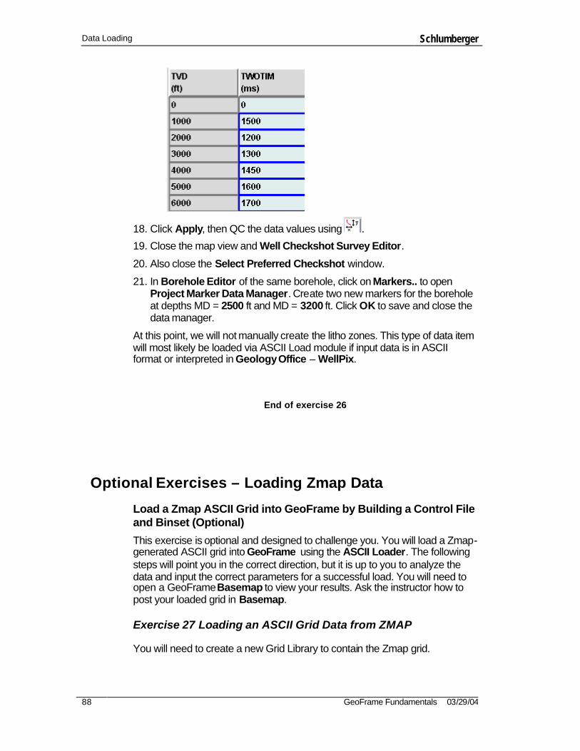
Data Loading Schlumberger
88 GeoFrame Fundamentals 03/29/04
18. Click Apply, then QC the data values using .
19. Close the map view and Well Checkshot Survey Editor.
20. Also close the Select Preferred Checkshot window.
21. In Borehole Editor of the same borehole, click on Markers.. to open Project Marker Data Manager. Create two new markers for the borehole at depths MD = 2500 ft and MD = 3200 ft. Click OK to save and close the data manager.
At this point, we will not manually create the litho zones. This type of data item will most likely be loaded via ASCII Load module if input data is in ASCII format or interpreted in Geology Office – WellPix.
End of exercise 26
Optional Exercises – Loading Zmap Data
Load a Zmap ASCII Grid into GeoFrame by Building a Control File and Binset (Optional)
This exercise is optional and designed to challenge you. You will load a Zmap- generated ASCII grid into GeoFrame using the ASCII Loader. The following steps will point you in the correct direction, but it is up to you to analyze the data and input the correct parameters for a successful load. You will need to open a GeoFrame Basemap to view your results. Ask the instructor how to post your loaded grid in Basemap.
Exercise 27 Loading an ASCII Grid Data from ZMAP
You will need to create a new Grid Library to contain the Zmap grid.
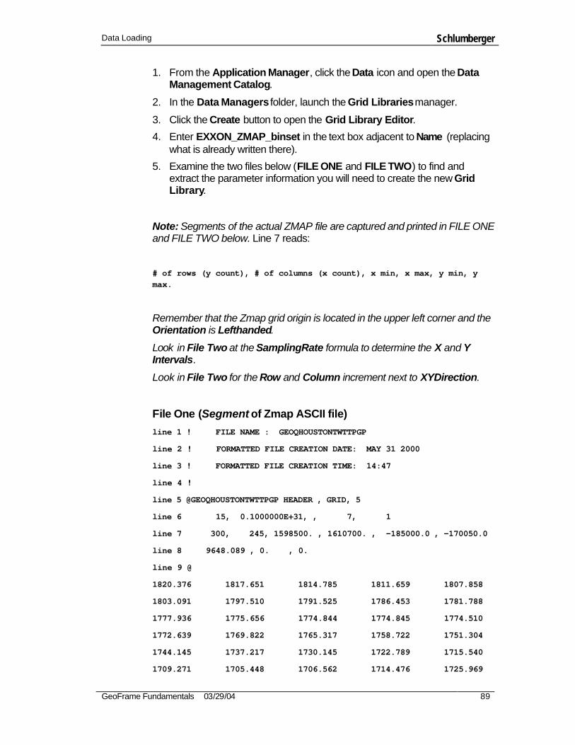
Data Loading Schlumberger
GeoFrame Fundamentals 03/29/04 89
1. From the Application Manager, click the Data icon and open the Data Management Catalog.
2. In the Data Managers folder, launch the Grid Libraries manager.
3. Click the Create button to open the Grid Library Editor.
4. Enter EXXON_ZMAP_binset in the text box adjacent to Name (replacing what is already written there).
5. Examine the two files below (FILE ONE and FILE TWO) to find and extract the parameter information you will need to create the new Grid Library.
Note: Segments of the actual ZMAP file are captured and printed in FILE ONE and FILE TWO below. Line 7 reads:
# of rows (y count), # of columns (x count), x min, x max, y min, y max.
Remember that the Zmap grid origin is located in the upper left corner and the Orientation is Lefthanded.
Look in File Two at the SamplingRate formula to determine the X and Y Intervals.
Look in File Two for the Row and Column increment next to XYDirection.
File One (Segment of Zmap ASCII file) line 1 ! FILE NAME : GEOQHOUSTONTWTTPGP
line 2 ! FORMATTED FILE CREATION DATE: MAY 31 2000
line 3 ! FORMATTED FILE CREATION TIME: 14:47
line 4 !
line 5 @GEOQHOUSTONTWTTPGP HEADER , GRID, 5
line 6 15, 0.1000000E+31, , 7, 1
line 7 300, 245, 1598500. , 1610700. , -185000.0 , -170050.0
line 8 9648.089 , 0. , 0.
line 9 @
1820.376 1817.651 1814.785 1811.659 1807.858
1803.091 1797.510 1791.525 1786.453 1781.788
1777.936 1775.656 1774.844 1774.845 1774.510
1772.639 1769.822 1765.317 1758.722 1751.304
1744.145 1737.217 1730.145 1722.789 1715.540
1709.271 1705.448 1706.562 1714.476 1725.969

Data Loading Schlumberger
90 GeoFrame Fundamentals 03/29/04
File Two (Segment of the zmap_grid_feet.ctl)
gal_CreateGridVector ZmapGrid
(
Precondition = (Tag1 == "@" &&
(ZmapGrid.ElementsRead < XCount * YCount)),
EndOfData = ZmapGrid.ElementsRead == XCount * YCount,
Container = HorizonDI,
LocalRecordLength = LengthOfEachValue*NumberOfValuesPerLine,
GridAbsentValue = ZmapAbsentValue,
PropertyColumn = 1,
WrapMode = 1,
PropertyCode = "Depth",
PropertyUnit = "ft",
Dimension = 2,
GridLibraryName = "Zmap",
GridCode = "SHAPE_2D",
GridName = "Zmap_Grid",
Rotation = {0.0},
FastestChangeDir = {2}, //Y major
XYDirection = {1,-1}, //upper left, x incr, y decr
Separator = "",
Start = {XMin,YMax}, //upper left
Count = {XCount, YCount},
SamplingRate = {XMax,YMin},//Will be calculate as {(XMax- XMin)/(XCount-1),(YMax-YMin)/(YCount-1)},
XYIndexUnit = "ft",
DataValues = {gal_Number(,," ","%g")},
);
gal_CreateString Tag1
(
Precondition = Gen.RealDataCurrentLine >= 3 && gal_String(1,1) == "@",
DataValues = {gal_String(1,1)},
Values = {Tag1.GetStrDataValue()[0]},
6. Once the Grid Library Editor parameters are completed, click OK to exit.
7. Click OK to exit the Project Grid Library Data Manager.

Data Loading Schlumberger
GeoFrame Fundamentals 03/29/04 91
Note: The grid parameters are now set.
Load the Zmap Grid into GeoFrame
8. From Application Manager select Data>Loaders and Unloaders, to
launch the ASCII Load module.
9. Click Input File and filter to the ZMAP file location (ask the instructor for the path).
10. Click Control File and enter EXXON_ZMAP.ctl in the Selection field, then click OK to close the window.
11. In the ASCII Load window, click the gray button next to Create Control File, and select Grid Set Data.
12. Click Create Control File to open the Grid Sets - Control File Builder window.
13. Fill in the ASCII Format Information, Property Information and Grid Information parameters.
Note: Step 6 requires that you think about the parameter settings!
14. In the Grid Information subwindow, enter EXXON_your initials in the Grid Name field.
Note: Check File Two for Fastest Changing Direction and X/Y Direction.
15. Click Target Surface and select the h horizon, then click OK to close.
16. Click Run to load the Zmap grid.
17. Toggle ON Grids in the ASCII Load module then click Manager(s)
Post the Zmap grid on the Basemap
18. Re-open Basemap if you have exited from it.
19. From the Basemap menu, select Post>Interpretation to open the Interpretation window.
20. Click Grids to open the Post Surface Data window.
21. Open the h horizon folder, open the Grid folder and select the EXXON_your initials grid.
22. Click OK to post into Basemap.
End of exercise 27


Data Save Schlumberger
GeoFrame Fundamentals 03/29/04 93
Chapter 6 Data Save
Overview
The Data Save module is used to write data from a GeoFrame project to disk, tape or network device in Archive, Geoshare, LIS, DLIS, or ASCII format.
Data Save archives the whole processing chain including the processing history and gives you control over what data you save, so you can use it to make user-controlled backups.
Keywords
Knowledge of the following keywords will help you to understand the concepts introduced in this chapter:
• GeoShare
• LIS
• DLIS
• ASCII
• Archive
• File Number
• File ID
• Snap
• Export
Data Save Format Options
There are five ways to format the data that you wish to save:
• GeoFrame Archive format has an underlying representation defined by the American Petroleum Institute’s Recommended Practice 66 (RP66). This format is used to save a selected project data in Archive format for safekeeping or to transfer via Data Load into another GeoFrame project.
• Geoshare format output generated consists of RP66 data. This format makes extensive use of private object types. Use the Geoshare format when you want to move from a GeoFrame project to a non-GeoFrame interpretation workstation that supports the Geoshare format.
• DLIS format output generated consists of RP66 data. This format is used to save only one borehole and its associated logical files. The primary

Data Save Schlumberger
94 GeoFrame Fundamentals 03/29/04
purpose of DLIS format is to produce data that can be processed by clients’ non-GeoFrame software.
• LIS (Log Information Standard) format is not RP66 data. It is a proprietary data exchange format that was defined by Schlumberger in the late 1970’s. The LIS formatted alias files are included to accommodate modified codes and other variables. Select LIS format only when specifically requested.
• ASCII format will generate a text file. The ASCII option utilizes a control file in which to refine the user’s selection and identify the information to be used. The control file also identifies which specialized ASCII format will be written.
Pre-built control files are provided for commonly used ASCII formats. The user may also create customized control files to generate specialized output formats.
Using Data Save
The operation in saving log curves in DLIS and LIS is very similar. This exercise gives you an example of procedures that allow you to save data to a file using DLIS format. You will also learn how you can utilize Inter-Task Communication from the General Data Manager to Data Save module.
Exercise 28 Exporting Log Data in DLIS Format
1. Open the Data Management Catalog by clicking on the Data icon in the Application Manager.
2. Select Data Save and click OK.
3. Click HELP in the bottom right corner of the Data Save window to open the Data Save User’s Guide Bookshelf document. Refer to this document for assistance with the exercises in this chapter.
4. In the Data Save window, set Destination as File, and set Format as DLIS.
5. Click Save as to open Select the Target File window then type in a name for the output DLIS file.
6. Open the ITC Door in Data Save.
7. In General Data Manager, expand the boreholes contained by Amber Field to get a list of log curves. You can also use the Query Tool to expand some log curves from the boreholes contained by Amber Field.

Data Save Schlumberger
GeoFrame Fundamentals 03/29/04 95
8. Highlight some of the log curves contained by a borehole then click the
ITC Broadcast icon . The selected log curves will appear in the Selection area of Data Save. Then Apply.
9. Type in the File Number to 1 and File Id to the borehole name then Apply.
10. Now go back to General Data Manager and highlight same codes of log curves contained by another borehole then broadcast them to Dave Save module with the ITC.
11. Click OK on the Confirm window. This will change the File Number from 1 to 2. Edit the File Id to show the second selected borehole then Apply.
12. Click Run.
Your DLIS data will be saved in your geoframe40x_sun folder, ready to import into other applications (or other instances of GeoFrame). If you want to check that it has worked properly, load the file or alternate, using Data Load.
Note: When DLIS or LIS format is chosen, Data Save does not allow a selection from more than one borehole per logical file.
End of exercise 28
Data Save - ASCII
Pre-built control files are provided for commonly used ASCII formats. You may create customized control files to generate specialized output formats.
Exercise 29 Exporting Grid Data
This exercise will demonstrate saving data as an ASCII file.
1. In Data Save module, select ASCII in the Format option. ASCII Save Format Options window will pop up showing a series of GeoFrame data types that can be output as ASCII.
2. Select GF_Ascii_Save_Grid from this window. Selecting this format will display the pre-built control file. Leave that as is.
3. Save the output file as Caracas_grid.ascii.
4. Ensure that you clear out any data items under Selection from the previous exercises. To do this:
• Highlight those data items under Selection then use to scissor icon to remove them.
5. In General Data Manager, expand the project level to list the horizons.
Data Save Schlumberger
96 GeoFrame Fundamentals 03/29/04
6. Highlight CARACAS_ASAP – Horizon then expand again to list the grids contained by this horizon. Double click on Caracas_asap_charisma_grid to find more information about this grid in the Grid Library Editor such as the XY origin, XY interval etc. When you are finished, close the editor and then broadcast the grid to Data Save module.
7. Click Run.
8. On your workstation, open a Text Editor window and briefly view your grid data.
9. Go back to Data Save module and then save out an ASCII – scatter set data from the same horizon, which is CARACAS_ASAP. View the result in the Text Editor window.
10. Exit from Data Save module.
End of exercise 29
Export Well Marker Data using Data Save and Modify the Marker Output Format
The first part of this exercise exposes you to the process of selecting marker data for export using the GeoFrame Marker Data Manager and ITC filter function, and using the Data Save module to export the file in ASCII format. The second part of the exercise will show you how you can modify the well_marker control file to produce a more condensed data output file.
Exercise 30 Exporting Well Marker Data
1. Re-open the Data Save module, if you have closed it.
2. Select the ASCII Format and pick Well Marker from the format options window.
3. In the General Data Manager, expand the project to list the wells contained by Amber Field.
4. In the Data Save window, open the ITC door.
5. In the Project General Data Manager window, click the ITC Broadcast icon to send the selected wells to the Data Save Selection area.
6. Save the ASCII file as Amber_markers.dat.
7. Click Run to export the data then view the marker data in the Text Editor window.
8. Examine the exported file in your home directory under the geoframe40x_sun subdirectory.

Data Save Schlumberger
GeoFrame Fundamentals 03/29/04 97
9. In the Data Save window, under Format Options, note the path to the well_marker.ctl file.
10. Open a Unix xterm window.
11. In the xterm window, navigate to the directory that contains the well_marker.ctl file, and copy the file to your home directory.
12. In order for us to modify the control file, enter: textedit well_marker.ctl or you can use the vi editor.
13. In the text editor, scroll down to locate and change gas_Block Header, BlockElements and IndexOptions in Script # 1 to read like the gas_Block Header, BlockElements and IndexOptions in Script # 2.
Script # 1
gas Block Header (Format= {“Well UWI Borehole UWI Marker Name Marker Type X Y Z\n”},);
BlockElements = {WellUWI, BoreholeUWI, MarkerName, MarkerSubType, WellMarkerLocation, CR},);
IndexOptions = {"MD"}, // default Z measurement // IndexOptions = {"MD,TVD,TVDSS,TWT"}, // all Z measurements);
Script # 2
gas Block Header (Format= {“ Borehole UWI Marker Name X Y Z\n”},);
BlockElements = {BoreholeUWI, MarkerName, WellMarkerLocation, CR},);
IndexOptions = {"MD, TVD, TWT"}, // default Z measurement // IndexOptions = {"MD,TVD,TVDSS,TWT"}, // all Z measurements);
14. When finished, save the new control file with a new name, i.e., TS_well_marker.ctl
15. In the Data Save window, select the Save As button and enter TS_Amber.dat
16. Click Control File and select the new control file you saved.
17. Click Run to export the modified ASCII file. Examine the exported file.
End of exercise 30

Data Match and Merge Schlumberger
GeoFrame Fundamentals 03/29/04 99
Chapter 7 Other Project Data Managers
Overview
You have been introduced to the use of several project data managers in the previous exercises. These project data managers allow you to list, modify, add, and delete information to and from the database.
Most of the Project Data Managers have similar interfaces consisting of:
• Spreadsheet display of data
• Lists that allow you to customize the specific data displayed
• Icons that provide short-cuts and paths to other data management objects
This chapter will further expand on the previous introductions and exercises that you have had for the Project Data Managers. During the course of the exercises, you will realize the functions that are consistent across all of the data managers, as well as learn those that are specific to a certain data type.
Interpretation Model Manager (IMM)
GeoFrame 4 introduces Interpretation Model Manager (IMM) that manages different interpretation states, for example, iterations in the interpretation.
An interpretation model is defined as a collection of horizons, faults, contacts, boundaries and boundary sets. The Interpretation Model Manager is used to browse, create and edit interpretation models.
Access the GeoFrame user guide to get more detailed information regarding the Information Model Manager.
The following is a hands-on exercise in creating a new interpretation model in Time, consisting of some horizon versions and faults.
Exercise 31 Using the Interpretation Model Manager
1. In the Interpretation Model Manager, click the Create button.
2. Enter a name for your new Time Model, then click OK.
3. Click Populate to open the Populate Interpretation Model window.
4. The Assign option is toggled ON by default, leave it as is. The first time model that you will create is to assign or clone the interpretation data.
5. Click the small triangle to list the available time interpretation models, and select Default.
6. Ensure that Horizon Versions, Fault Cuts, Contacts and Fault Boundaries are toggled ON.
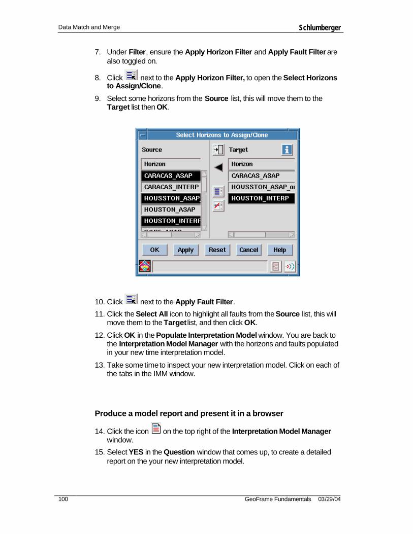
Data Match and Merge Schlumberger
100 GeoFrame Fundamentals 03/29/04
7. Under Filter, ensure the Apply Horizon Filter and Apply Fault Filter are also toggled on.
8. Click next to the Apply Horizon Filter, to open the Select Horizons to Assign/Clone.
9. Select some horizons from the Source list, this will move them to the Target list then OK.
10. Click next to the Apply Fault Filter.
11. Click the Select All icon to highlight all faults from the Source list, this will move them to the Target list, and then click OK.
12. Click OK in the Populate Interpretation Model window. You are back to the Interpretation Model Manager with the horizons and faults populated in your new time interpretation model.
13. Take some time to inspect your new interpretation model. Click on each of the tabs in the IMM window.
Produce a model report and present it in a browser
14. Click the icon on the top right of the Interpretation Model Manager window.
15. Select YES in the Question window that comes up, to create a detailed report on the your new interpretation model.

Data Match and Merge Schlumberger
GeoFrame Fundamentals 03/29/04 101
16. When you have the browser open, click the contents under Table of Contents that you wish to view.
End of exercise 31
Interpretation Data Manager
Interpretation Data Manager is also called the Surface Data Selector (in Standalone GeoFrame project) that has a purpose to select surface data and communicate your selection to the target. This Interpretation Data Manager can also be launched from Charisma, IMain, InDepth, SeisClass and Interpretation Model Manager.
Exercise 32 Using the Interpretation Data Manager
1. Highlight CARACAS_ASAP in the Interpretation Model Manager. Notice that the three buttons on the bottom of the window are activated.
2. Click Computed Data, this will open the Interpretation Data Manager.
3. The Context will show: Computed from interpretation data that list all data types computed from the CARACAS_ASAP horizon.
List all of the Grids in the Project
4. Click at the top right of the Interpretation Data Manager and select Project. This will list all types of the interpretation data in your GeoFrame project.
5. Toggle on Filter, then click the user filter icon .
6. Resize the size of the window so you can see the data displayed under Filter.
7. Toggle on the Type button next to Grid.
8. Configure the display table by clicking on .
9. Select Horizon Version from the Available Columns. This will move it to Visible Column automatically.
10. Select Create Date from the Visible Columns and move it to the
Available Columns using . If you wish, you can also adjust the priority of columns using the UP and DOWN arrows.
11. Click OK to close the Table Configuration window.

Data Match and Merge Schlumberger
102 GeoFrame Fundamentals 03/29/04
Generate a HTML based list
1. Highlight the following grid names:
Caracas_asap_twt_grid
Houston_asap_charisma_grid
Kobe_asap_charisma_grid
Paris_asap_charisma_grid
2. Click and select YES in the Question window.
3. After you are done seeing the report in the browser, close the Interpretation Data Manager, Interpretation Model Manager and the browsers.
End of exercise 32
Horizon Patch Data Manager
The Horizon Patch concept allows you to store individual parts of the same thrust-faulted horizons from your interpretation model as patches, under a single horizon name. The Horizon Patch Data Manager helps you filter the patches according to the interpretation model present in your project.
Exercise 33 Using the Horizon Patch Data Manager
To demonstrate how Horizon Patch concept works in a seismic window, the instructor will show you how a horizon patch is created in IESX or Charisma. Briefly, the procedures to add a new patch in IESX is as follows:
1. In IESX > Seis3DV/2DV, click MB3 > H List… to open Active Selection window. By default the active horizon is h.
2. Click on the Patch Options then click Add New Patch for horizon h. Keep the Active Selection window open.
3. Highlight patch 1 for horizon h, interpret the horizon in seismic window. To break, MB3> Break.
4. To interpret another patch, highlight the patch 2 for horizon h and then continue interpreting in seismic window.
Access the Project Horizon Patch Data Manager from the Data Management catalog.
5. In the Project Horizon Patch Data Manager, click the Interpretation Model under Table Setup.

Data Match and Merge Schlumberger
GeoFrame Fundamentals 03/29/04 103
6. Select the interpretation model that you created in the previous exercise. It will give you a list of horizons with Patch Order 0.
7. Assume that CARACAS_ASAP has some points, which intersect with the reverse faults. The GeoFrame seismic applications or Horizon Patch Data Manager allow you to create another patch to handle multiple Z values.
8. Click the Add button and add two rows.
9. Enter the new names on each row then highlight the new rows.
10. Select the Target Horizon: CARACAS_ASAP
11. Click Apply.
12. Click Reorder then OK. You will see the newly added horizon patches displayed in the order of the Patch Order.
13. Close the Project Horizon Patch Data Manager.
End of exercise 33
Project Zone Version Data Manager
A Zone Version is a collection of Zone Sets, which contains a set of non-overlapping zones. A borehole may contain one or more Zone Sets, but only one Zone Set per borehole per Zone Version.
Zone Versions enable the use of overlapping zones. Zone Versions will allow a user to create litho zones of different granularity. For example one Zone Version may contain a zone covering the entire Cretaceous section of a well, a second Zone Version may contain zones for each lithostratigraphic unit, a third Zone Version may contain zones for individual sands, and finally a fourth Zone Version may contain separate zones for the gas-, oil-, and water-bearing portions of a reservoir.
Several data managers now require that you specify a target zone version before you can manipulate data. Use Project Zone Version Data Manager to create, edit, delete, copy and merge zone versions.
Exercise 34 Using the Project Zone Version Data Manager
1. Open Project Zone Version Data Manager on the primary screen and Project Litho Zone Data Manager on the secondary screen.
2. In Project Zone Version Data Manager, create a new zone version. Ensure that no zone version is highlighted and Create/Edit tab is selected. Type in a name then Apply. A new and empty zone version will be created.
Data Match and Merge Schlumberger
104 GeoFrame Fundamentals 03/29/04
3. To rename a zone version, highlight any existing zone version then type in the new name and Apply. Now you should see the difference between creating a new and re-naming zone version.
4. In the Project Litho Zone Data Manager, select the new zone version from Target Zone Version. It should be empty.
5. Go back to Project Zone Version Data Manager and you will add zone sets into the new and empty zone version.
6. Under Select Borehole(s), highlight the new and empty zone version then click Add/Remove Zone Sets. The Zone Sets contained by the selected boreholes will appear under Select Zone Set(s).
7. Under Select Zone Set(s), select which zone sets you wish to include in your new zone version. Hint: the program allows you to select only one zone set per borehole per zone version.
8. Click OK when you are finished then inspect the litho zones that you picked from the selected zone sets in Project Litho Zone Data Manager.
Merge Litho Zones from Two Zone Versions
You can merge two or more existing zone versions to create a new zone version, or you can merge one or more existing zone versions into another zone version that already exists.
9. Select the Copy/Merge tab in the Project Zone Version Data Manager.
10. Select the zone versions you wish to merge. Use the CTRL key to select multiple zone versions.
11. Toggle ON Target Zone Version, then type in a name and Apply.
End of exercise 34
NOTE: If two or more of the zone versions you intend to merge have the same borehole or zone set associations, the merged zone version takes the associations of the source zone version that was chosen first.
Drill Stem Test Data Manager
The project does not have any drill stem test (DST) data, so you will need to load or manually enter the DST data to be able to view the data in the Project Drill Stem Test Data Manager. A simple DST data set has been created for you to load using the ASCII Loader. The file name is DST.dat (your instructor should tell you the location of the data). The file contains DST data for borehole Agate-H6 and Diamond-14 consisting of three DST attributes (Fluid Resistivity, Well Head Flowing Pressure, and Choke). By now, you should be familiar with using the ASCII Loader.
Data Match and Merge Schlumberger
GeoFrame Fundamentals 03/29/04 105
Exercise 35 Using the Drill Stem Test Data Manager
1. Open the ASCII Loader from the Data Management Catalog.
2. Select the input file, which is DST.dat, from the location given by your instructor.
3. Change the Control File to Drillstem Test Data then start defining the control file in the Control File Builder window.
Note: Remember that this file contains DST for multiple boreholes, you will need to toggle ON the Multi Borehole UWI option in the Control File Builder window.
4. When the loading is complete. Toggle on the Drillstem Tests option on the bottom right of the ASCII Loader window then click the Manager(s) button.
5. View the DST data that you loaded. If you wish, you can assign the Layer for each of interval name.
6. Close the Project Drillstem Test Data Manager.
7. Exit from the ASCII Loader.
End of exercise 35
Project Core Data Manager
Access the Project Core Data Manager from the Data Management catalog. Since there is no core data in your project, so you will require loading some, then enter the attribute values for the core. The core image file name is core_image.JPEG. ASCII Load can load core images in almost any type of image format (TIFF, GIF, JPEG, etc.). The ASCII Loader also allows you to load the core attributes and core arrays.
Exercise 36 Using the Project Core Data Manager
1. Open the ASCII Loader from the Data Management Catalog.
2. Select the input file(s) from the location given by your instructor.
3. Change the control file to Core Image Data, then click the Create Control File .
4. Under the Loading Information, select Unrolled for the Core Image Scan Type .
5. Under Image Information, enter Top Depth: 5000 ft.; Bottom Depth: 5060 ft.
Data Match and Merge Schlumberger
106 GeoFrame Fundamentals 03/29/04
6. Click the Display button to open the Core Image Editor. Take a brief look on the core image by scrolling up or down. In this window, you can crop, rotate, zoom in and zoom out the core image. If you wish, experiment with what you can do in this window. To go back to the original core image, click Reset.
7. Click OK to close the Core Image Editor.
8. Click OK in the Core Image – Control File Builder.
9. In the ASCII Loader window, click the Target Borehole UWI and select Diamond-14. Then click RUN.
10. Go back to the Project Core Data Manager, and click the Cores button.
11. Select CoreInterval_xxxxxx, and then click OK.
12. If you wish, you can modify the displayed attributes by clicking on Attributes.
13. Enter the values for the following core attributes:
Bulk Density (g/cm3) 2.52
Permeability (mD) 50
Porosity (ft3/ft3) 38
Water Saturation (ft3/ft3) 75
Oil Saturation (ft3/ft3) 12.5
14. Click OK to save the values to the database.
End of exercise 36
You should be familiar with the different data managers and be comfortable navigating around within them and manipulating or viewing data.
The completion of the Data Manager exercises marks the end of the introduction to GeoFrame and the Fundamental functionality of the Project Manager, the Process Manager, and the Data Manager utilities. At this point in the course you should be comfortable with creating a new project and populating it with different types of well data.
The rest of the course will build on the skills you have learned. You will apply all of your new GeoFrame skills to create a practical environment that will utilize some of the additional functionality that was mentioned, but not practiced, so far in the course, such as the shared project concept.

Data Match and Merge Schlumberger
GeoFrame Fundamentals 03/29/04 107
Posting Well Data in Geology Office – Composite
Geology Office is a suite of highly integrated geological applications that can be launched in context with each other. It contains basic as well as advanced tools including WellPix, Composite , Cross Section, WellEdit, WellComposite, ResSum, GeoViz , LithoToolKit and GeoPlot.
The following exercise will be introduced and demonstrated by your instructor to show you that the well data you loaded previously can be posted in a Geology Office - Composite very easily. Details on how to use the applications in Geology Office are introduced in a Geology Office two-day course.
Exercise 37 Posting Well Data in Geology Office – Composite Window
1. Open Geology Office . Go to Application Manager > Geology Office .
2. In Geology Office launching bar, click on Composite.
3. Select a borehole (Agate-H6). Type in a name for a new composite.
4. Create tracks for Markers, Production Data and Core.
5. Double click on each track to launch its edit window then post the data.
• Markers are usually posted automatically once the marker track is
created; otherwise use the open folder icon to add markers from database.
• To post production data (DST or Completed Interval), you have to
open the Production Edit window then click .
• To display core, open the Core Edit window and use or you may also create it graphically.
End of exercise 37