University of South CarolinaScholar Commons

Faculty Publications Earth and Ocean Sciences, Department of

5-6-2004

Geomorphic Analysis of Tidal Creek NetworksKaryn Inez Novakowski

Raymond Torres

L Robert Gardner

George VoulgarisUniversity of South Carolina - Columbia, gvoulgaris@geol.sc.edu

Follow this and additional works at: http://scholarcommons.sc.edu/geol_facpubPart of the Earth Sciences Commons

This Article is brought to you for free and open access by the Earth and Ocean Sciences, Department of at Scholar Commons. It has been accepted forinclusion in Faculty Publications by an authorized administrator of Scholar Commons. For more information, please contactSCHOLARC@mailbox.sc.edu.

Publication InfoPublished in Water Resources Research, Volume 40, Issue W05401, 2004, pages 1-13.Novakowski, K. I., Torres, R., Gardner, L. R., & Voulgaris, G. (2004). Geomorphic analysis of tidal creek networks. Water ResourcesResearch, 40 (W05401), 1-13.© Water Resources Research 2004, American Geophysical Union

Geomorphic analysis of tidal creek networks

Karyn Inez Novakowski, Raymond Torres, L. Robert Gardner, and George Voulgaris

Department of Geological Sciences, University of South Carolina, Columbia, South Carolina, USA

Received 2 October 2003; revised 7 January 2004; accepted 26 January 2004; published 6 May 2004.

[1] The purpose of this study is to determine if concepts in terrestrial channel networkanalysis provide insight on intertidal creek network development and to present newmetrics for their analysis. We delineated creek network geometry using high-resolutiondigital images of intertidal marsh near Georgetown, South Carolina. Analyses reveal thatintertidal creek networks may be topologically random. Length-area relationshipssuggest that salt marsh and terrestrial networks have similar scaling properties, althoughthe marsh networks are more elongate than terrestrial networks. To account forrecurrent water exchange between creek basins at high tide, we propose that the landscapeunit of geomorphic analyses should be the salt marsh island as opposed to salt marsh creekdrainage basin area. Using this approach, the relationship between maximum channellength per island and island area is well described by a power function. A similar powerrelationship exists for cumulative channel length versus island area, giving a nearlyunit slope; this implies that marsh islands have a spatially uniform drainage density. Sincethe island boundaries are easily identified in remote sensing, taking the island as the unitof geomorphic analysis will eliminate discrepancies in delineating basin boundariesand preclude the need for defining basin area in intertidal landscapes. Analyses and resultspresented here may be used to quantify salt marsh reference condition and provideindicator variables to assess salt marsh disturbance. INDEX TERMS: 1824 Hydrology:

Geomorphology (1625); 1848 Hydrology: Networks; 1640 Global Change: Remote sensing; KEYWORDS:

drainage areas, geomorphology, islands, networks, salt marsh

Citation: Novakowski, K. I., R. Torres, L. R. Gardner, and G. Voulgaris (2004), Geomorphic analysis of tidal creek networks, Water

Resour. Res., 40, W05401, doi:10.1029/2003WR002722.

1. Introduction

[2] Estuarine and intertidal environments are sedimentsinks with complex hydrodynamic processes that producespatially variable deposition and erosion [e.g., Pestrong,1965; Leonard, 1997; Fagherazzi and Furbish, 2001].Sediment accumulation leads to mudflat formation, withsalt marsh at higher elevations [Redfield, 1972; Allen andPye, 1992]. Typically, tidal creek networks etch the saltmarsh surface, becoming dry at low tide. These small-scalechannels facilitate inundation and drainage of marshlandsand they control, to a large extent, estuary-wide hydrody-namics [Pestrong, 1965; Rinaldo et al., 1999a]. Moreover,marsh channel networks control mass and energy exchangewith the coastal ocean and therefore help sustain high saltmarsh productivity; they also provide critical habitat foreconomically important fish. Hence salt marsh landscapesare the geographic templates upon which highly productiveintertidal ecosystems function, and in order to understandthe development and stability of salt marsh systems animproved understanding of salt marsh landforms is required.[3] Early work on intertidal zone geomorphology was

focused on the hydraulic geometry of estuarine channels.Results from these efforts indicate that intertidal channelsexhibit an exponential decrease in width in the upstreamdirection, and that this change in geometry facilitates greater

tidal energy dissipation through the channel network byincreased friction [Myrick and Leopold, 1963; Langbein,1963; Wright et al., 1973]. Pestrong [1965] favors theHorton [1945] model of channel development for intertidalchannels with the important distinction that marsh incisionoccurs during the higher velocity ebb flows. Pestrong alsorecognized that microtopography may control channel ini-tiation by concentrating sheet flow, and some tributariesmay experience predominantly unidirectional flow. He wenton to reason that some channels be characterized as terres-trial, influenced by their contributing areas.[4] Subsequent marsh geomorphic research has focused

on planform geometry. Geyl [1976] attempted to linkchannel network characteristics to tidal channel basin area.He used air photos and small-scale maps to characterize thestability of channel networks. Although the main findingsare inconclusive, Geyl’s analyses represent an early attemptat using drainage basin area to compare terrestrial andestuarine channel networks.[5] Wadsworth [1980] conducted detailed studies of

drainage density and channel reticulation in the tidal DuplinRiver system. Like Geyl [1976], Wadsworth used theseanalyses to infer marsh network stability. Wadsworth rea-soned that network boundary conditions and local slope areprimary controls on network evolution, and that channellength is more responsive to tidal forcing than contributingarea of the individual tidal basins. Collins et al. [1987]presented the first detailed description of marsh morphologyby evaluating the topography of a 4.5 ha section of marsh

Copyright 2004 by the American Geophysical Union.0043-1397/04/2003WR002722

W05401

WATER RESOURCES RESEARCH, VOL. 40, W05401, doi:10.1029/2003WR002722, 2004

1 of 13

area within the 30 km2 Petaluma River Estuary. They foundthat biogenic and physical processes interact and are indelicate equilibrium with marsh morphology. They alsoreasoned that tidal prism continuity drives geomorphicevolution in marsh landscapes, and went on to infer thatterrestrial concepts of drainage basin evolution apply tointertidal marsh environments. They did not, however, useterrestrial geomorphic indices to evaluate marsh geomor-phology (e.g., contributing area - channel length).[6] Pethick [1992] reasoned that salt marshes should be

regarded as the landward extension of mudflat systems, andthat salt marshes self-adjust in response to storm perturba-tions. Pethick also suggested that some marsh channels mayhave resulted fromflood tide inundation, as opposed to the ebbtide drainage model of Pestrong [1965]. These findings mayunderlie the observation byMarani et al. [2003] that drainagedensity is not a diagnostic feature of salt marsh landscapes.[7] Despite the vastly different environmental conditions,

field observations reveal that intertidal channel networksbear a strong resemblance to those of terrestrial systems[e.g., Pestrong, 1965; Knighton et al., 1992; Pethick, 1992].Cleveringa and Oost [1999] support this contention byproviding evidence for ‘‘statistical self-similarity’’ in tidalbasin channel networks, a common feature of terrestrialchannel systems. On the other hand, Ragotzkie [1959]observed that marsh basin networks in a region of uniformtidal range were highly variable. This general finding issupported by Fagherazzi et al. [1999]; their nonlinear plotsof marsh basin area-channel length indicate that tidalchannel networks are not scale-invariant, unlike most ter-restrial channel networks.[8] Typically, landscape evolution models assume that

landscape forming discharges (Q) are proportional to thewatershed contributing area (A) that is defined by topogra-phy (i.e., Q / A). Rinaldo et al. [1999a] used a linearizedversion of the governing flow equations to model watersurface topography during high tide. They exploited theQ / A assumption by redefining the contributing areasusing flow divides associated with the free water surface(energy slope) rather than area defined by topography oftidal basins. Rinaldo et al. [1999a] used their model resultsto test for scale invariance and they concluded that terres-trial models of geomorphic evolution do not apply to tidalbasin geomorphology.[9] Subsequently, Rinaldo et al. [1999b] tested for scale

invariance by linking water surface topography to maximumdischarge as estimated by the linearized hydrodynamicmodel. They found power law relationships between channelcross-sectional area, drainage area, tidal prism and peakdischarge at spring tides. However, their power law modelshold only for larger channels with a cross-sectional areagreater than 50 m2; below that the power law relationshipdoes not apply. This finding was attributed to inadequatespatial resolution of the digital terrain model, and to theassumptions included in their hydrodynamic modeling thatmade it inappropriate for smaller channels. Fagherazzi andFurbish [2001] suggested that the break in the power lawscaling is the result of increased sediment shear resistancewith substrate depth. In their work on the intertidal channelnetworks of the Venice Lagoon, Marani et al. [2003] foundthat there are regional differences in the dependence of totalchannel length on the volume of the tidal prism but uniform-

ity in the correlation of total channel length with watershedarea. These findings led them to suggest that the volume ofthe tidal prism is not a major control on channel networkgeometry.[10] Together these studies reveal that a consensus on the

role of hydrodynamic processes on intertidal geomorphol-ogy, scaling of geomorphic features, and what constitutesintertidal basin boundaries is lacking. Here, we quantify theplanform geomorphic properties of intertidal channel pat-terns using high-resolution (0.7 m � 0.7 m) digital imagery.The purpose of this study is to determine if concepts interrestrial channel network analysis provide insight onintertidal creek network structure and development, topresent new metrics for their analysis, and to evaluaterandomness in network topology. This latter goal is impor-tant because a positive result may establish a foundation forusing terrestrial concepts in the intertidal zone. Moreover,geomorphic metrics evaluated in this study may be used toguide salt marsh reconstruction efforts and serve as indica-tors for marsh disturbance.[11] Here basin and network analyses are limited to those

landscapes wholly within the intertidal zone, the small-scaledrainage basin areas that do not intersect the terrestriallandscape. This distinction is important because we endeavorto evaluate the effects of recurrent tidal forcing and sub-sequent material fluxes on salt marsh geomorphology(and to a lesser extent the effects of low tide rainfall events[e.g., Torres et al., 2003]). Although results presented heremay be site specific, the analyses and main findings mayprovide a framework for salt marsh landscape analysis thatapply to other intertidal environments.

2. Study Site

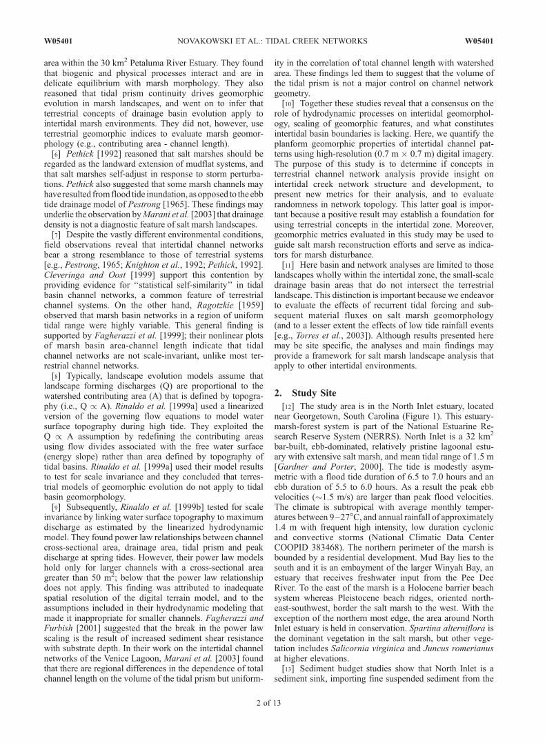
[12] The study area is in the North Inlet estuary, locatednear Georgetown, South Carolina (Figure 1). This estuary-marsh-forest system is part of the National Estuarine Re-search Reserve System (NERRS). North Inlet is a 32 km2

bar-built, ebb-dominated, relatively pristine lagoonal estu-ary with extensive salt marsh, and mean tidal range of 1.5 m[Gardner and Porter, 2000]. The tide is modestly asym-metric with a flood tide duration of 6.5 to 7.0 hours and anebb duration of 5.5 to 6.0 hours. As a result the peak ebbvelocities (�1.5 m/s) are larger than peak flood velocities.The climate is subtropical with average monthly temper-atures between 9–27�C, and annual rainfall of approximately1.4 m with frequent high intensity, low duration cyclonicand convective storms (National Climatic Data CenterCOOPID 383468). The northern perimeter of the marsh isbounded by a residential development. Mud Bay lies to thesouth and it is an embayment of the larger Winyah Bay, anestuary that receives freshwater input from the Pee DeeRiver. To the east of the marsh is a Holocene barrier beachsystem whereas Pleistocene beach ridges, oriented north-east-southwest, border the salt marsh to the west. With theexception of the northern most edge, the area around NorthInlet estuary is held in conservation. Spartina alterniflora isthe dominant vegetation in the salt marsh, but other vege-tation includes Salicornia virginica and Juncus romerianusat higher elevations.[13] Sediment budget studies show that North Inlet is a

sediment sink, importing fine suspended sediment from the

2 of 13

W05401 NOVAKOWSKI ET AL.: TIDAL CREEK NETWORKS W05401

Figure 1. ADAR image shows location and geography of North Inlet. The study area is outlined inblack. See color version of this figure at back of this issue.

W05401 NOVAKOWSKI ET AL.: TIDAL CREEK NETWORKS

3 of 13

W05401

Atlantic Ocean and Winyah Bay [Gardner et al., 1989;Vogel et al., 1996]. The inorganic fraction accounts for 80–85% of the accumulating mass [Gardner and Kitchens,1978; Vogel et al., 1996]. The organic fraction (15–20%)is derived from a variety of sources that include remains ofalgae, animals, microbes, terrestrial vegetation and marshplants [Goni and Thomas, 2000], the latter mainlyS. alterniflora. 137Cs analyses show that local annual aver-age sediment accumulation rates range from 1.3–2.5 mm/yr

[Sharma et al., 1987]. This accumulation rate is comparableto the local sea level rise rate of 2.2–3.4 mm/yr; hence themarsh surface is rising with sea level [Vogel et al., 1996].[14] The extensive salt marsh system has numerous well-

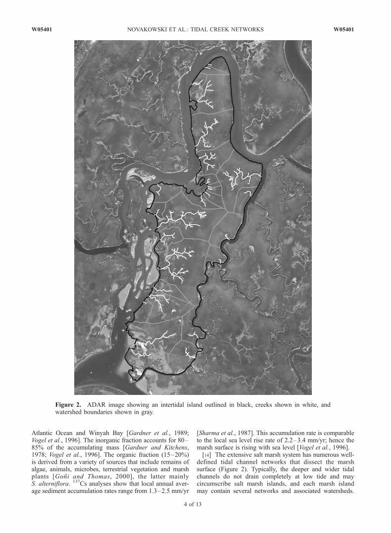
defined tidal channel networks that dissect the marshsurface (Figure 2). Typically, the deeper and wider tidalchannels do not drain completely at low tide and maycircumscribe salt marsh islands, and each marsh islandmay contain several networks and associated watersheds.

Figure 2. ADAR image showing an intertidal island outlined in black, creeks shown in white, andwatershed boundaries shown in gray.

4 of 13

W05401 NOVAKOWSKI ET AL.: TIDAL CREEK NETWORKS W05401

These smaller channel networks incise the marsh platformand become ‘‘dry’’ at low tide. The analyses presented hereare focused on the latter, smaller scale salt marsh creeknetworks, excluding the marsh creek networks that extendinto purely terrestrial environments. Therefore this researcheffort is directed at quantifying metrics for intertidal land-scapes with recurrent marine forcing.

3. Methods

[15] The base image for this study was acquired with anAirborne Data Acquisition and Registration (ADAR) 5500digital camera system with multispectral (blue, green, red,near IR) band widths (Figure 1). The image was obtained onNovember 4, 1999 from an altitude of 2763 m, close to solarnoon and low tide to limit sun angle and tidal inundationeffects, yielding a spatial resolution of approximately 0.7 �0.7 m [Jensen et al., 2002]. Creek networks (Figure 2) weredelineated by visually comparing percent reflectance ofS. alterniflora, water, and the gray to black, organic richmarsh mud. Water absorbs incident light reflecting 0–4%,marsh grass 5–50%, and mud 15–20% [Jensen, 2000].Reflectance differences between grass, water, and marshmud facilitates the delineation of the channel networks onthe marsh surface. Typically, the creek bed and inner banksare devoid of vegetation thereby facilitating delineation ofthe mid-channel. Field observations at low tide reveal thattidal creek networks that etch the marsh platform typicallydo not have flowing water greater than a few millimetersdepth or a few centimeters of standing water, or they may becompletely dry. These tidal creeks are distinct from thelarger tidal channels that typically retain >1 m of standingwater at low tide and thereby form salt marsh islands.[16] Analyses show that most creek networks, those

becoming ‘‘dry’’ at low tide, are ideal in the sense that theyhave no lakes, islands, or junctions with more than twotributaries. Some networks, however, were not delineatedand excluded from further analysis because they containedreticulating drainage systems, thereby precluding use ofconventional terrestrial network metrics. Reticulating creeknetworks diverge in the downstream direction and laterrejoin [Wadsworth, 1980]. The following properties weredetermined for each segment of each non reticulating creeknetwork, in ArcView: link length (l) and link magnitude (m,where link refers to a first order stream segment), Strahlerstream order (w), maximum stream length (L, the longeststream from the outlet to the source point), total channellength (SL), watershed area (Aw) and island area (AI). Wealso evaluated the frequency of topologically distinct creeknetwork types [e.g., Shreve, 1974].[17] A topologically random network is a network in

which all topologically distinct sub-networks of equalmagnitude occur with equal probability [Shreve, 1974].The number of topologically distinct networks for a givennumber of sources, is given by

N Mð Þ ¼ 2M � 2ð Þ!M ! M � 1ð Þ! ð1Þ

where M is the number of sources. Randomness was testedby counting the number of times that each topologicallydistinct sequence occurred and comparing it to the expected

value using a chi-squared (ca2) test where a = 0.05, degrees

of freedom = k � 1, where k is the number of categories. Ac2 test is a measure of how much an observed valuedeviates from an expected value. Here it is assumed thatnetworks are topologically random if each possiblesequence occurred with equal probability, or expectedvalues equaled observed values. If cobserved

2 is greater thanca2 then the hypothesis that marsh creek networks are

topologically random is rejected.[18] As described above, an island is a section of marsh

circumscribed by tidal channels that maintain >1 m of waterat low tide. Island boundaries were identified in the samemanner as tidal creeks, visual inspection of reflectancebetween marsh grass and mud in surrounding channels.Island areas (AI) were then determined with ArcView.Watershed area (Aw) is that area encompassing an individual,discrete creek network. Watershed areas were determined bya Theissen polygon method using end points of first ordercreeks, essentially assuming the watershed boundary is onehalf the distance between end points of first order creeks inneighboring basins, and mid points between adjacent creekmouths. The Theissen polygon results were compared toresults from manually delineating watershed boundaries for22 creek networks on a marsh island (Figure 2). Thegraphical comparison has a slope of 0.95 and r2 = 0.96,indicating that there is not a significant difference betweenthe two methods. Therefore the automated method was usedto avoid ambiguity in Aw delineation.

4. Results

[19] The study area is an 8.67 km2 portion of the NorthInlet intertidal marsh (Figure 1). In this mapped region thedeeper and wider intertidal channels retain water at lowtide, and consequently circumscribe 56 marsh islands. Wedelineated the intertidal channel networks on these islands;there were 725 in total. Maximum channel lengths andassociated network watershed areas ranged from 3 m to10654 m, and 127 m2 to 609418 m2, respectively. Approx-imately 94% of the networks had a terrestrial networkappearance; this means that in the downstream direction,channel segments converge toward a main channel. On theother hand, approximately 9.1 km or 6% of total channellength was classified as being part of a reticulating drainagesystem.

4.1. Stream Order

[20] The nonreticulating networks were less than or equalto Strahler stream order 5 (Table 1). Total number of streamsegments decline exponentially from 3254 first order seg-ments to 20 of order 5. Applying Horton’s laws of drainagecomposition, order (w) versus number of stream and meanstream length (lm) reveals an exponential trend that issimilar to those found in terrestrial systems. Figure 3contains data from this study together with data from eightother studies, three from terrestrial systems and five fromthe coastal zone. Some of the terrestrial and intertidal trendsin these data overlie each other despite differences in scalefrom which the data points were extracted and processescontrolling network development. The logarithmic relation-ship is y = AeBw where y is the number of channels of agiven order, and w is stream order, A is the y intercept, and Bis the slope of the line (Table 2). The minimum correlation

W05401 NOVAKOWSKI ET AL.: TIDAL CREEK NETWORKS

5 of 13

W05401

coefficient, r2, for these curve fits is 0.95 (data from NorthInlet). These high correlation coefficients indicate that theexponential model adequately describes changes in streamfrequency with order.[21] Mean stream segment length exponentially increases

with order (Horton’s law of stream order) although there aredistinct differences in the trends between terrestrial andcoastal networks (Figure 4). For example, the terrestrialdata illustrate a nearly uniform positive slope and higher r2

values (Table 2). The coastal data on the other handare different in two ways. First, the Wadsworth [1980],Pestrong [1965], and Pethick [1980] data show a uniformslope between orders 1–4, well described by an exponentialfunction, with slopes comparable to the terrestrial systems(Table 2). At order 5 however, there is an abrupt break inslope due to a lower than expected channel length. This lowvalue for mean channel length may be due to undersampling of order 5 channels. For example, Pestrong reports4 order 5 channels and both Wadsworth and Pethick have1 order 5 channel. Secondly, the slope of the Myrick andLeopold [1963] data is greater than the terrestrial trendslope, while the slope for the North Inlet data is lower.Together these data show that mean channel length is highlyvariable. Also, these exponential relationships (Figures 3and 4) are consistent with Horton’s law of stream numbersand lengths, and they are consistent with expectations from

Kirchner [1993] who showed that Horton ratios are insen-sitive to network structure.

4.2. Link Magnitude

[22] Discrete channel networks had link magnitudes (m)ranging from 1 to 229 (Table 3), with a total of 3254magnitude 1 channels comprising 58.6 km, and 896 mag-nitude 2 channels comprising 20.8 km. Therefore magnitude1 channels comprise 57% of all channels, and 45% of totalchannel length, magnitude 2 channels comprise 16% and16%, respectively. As Shreve [1969] noted and Kirchner[1993] confirmed, stream order analyses (e.g., Horton laws)lack sensitivity to detect substantial differences in geomor-phic character. As a consequence, we propose that semilog-arithmic plots of magnitude versus frequency and meanchannel length may yield insight on systematic variations innetwork structure.[23] Figure 5 shows that stream frequency declines as a

power function from magnitude 1 to magnitude 33, butthereafter scatter about the curve fit increases substantially.Also, over the range of magnitude 34 to 93 there are 14 linkmagnitude values that have a single occurrence, and12 channel networks with magnitude >93 have a singleoccurrence. On the other hand, mean channel length showsan increase over the same range in magnitude, but the scatter

Table 1. Count, Sum, and Mean Stream Lengths for a Given

Order for All Networks

Order Length Count Total Length, m Mean Length, m

1 3254 58588 18 ± 162 1613 42749 26 ± 343 614 22938 37 ± 374 145 6833 47 ± 435 20 1049 52 ± 32

Table 2. Summary of Slope B Values of Marsh and Terrestrial

Networks for the Function y = AeBw

Study Bcount rcount2 Bmean length rmean length

2

North Inlet �1.23 0.95 0.27 0.94Wadsworth [1980] �1.31 0.99 0.25 (�0.79) 0.09 (�0.95)Pestrong [1965] �1.35 0.99 0.73 (�1.0) 0.48 (�0.99)Myrick and Leopold [1963] �1.08 0.97 1.33 0.99Pethick [1980] �1.33 0.99 0.38 (�0.79) 0.13 (�0.95)Zeff [1999] �1.27 0.99 1.01 0.99Brush [1961] �1.20 0.99 1.01 0.99Valdes et al. [1979] �1.25 0.99 0.89 0.98Horton [1945] �1.22 0.99 0.76 0.92

Figure 3. Stream order (w) versus the number of streamsfor terrestrial and marsh networks (Horton’s law of streamnumbers). Marsh data are open symbols, and terrestrial dataare solid symbols.

Figure 4. Stream order (w) versus the mean segmentlengths (lm) for marsh and terrestrial networks (Horton’s lawof stream lengths). Marsh data are open symbols, andterrestrial data are solid symbols. Standard errors on eachmean value are represented by error bars.

6 of 13

W05401 NOVAKOWSKI ET AL.: TIDAL CREEK NETWORKS W05401

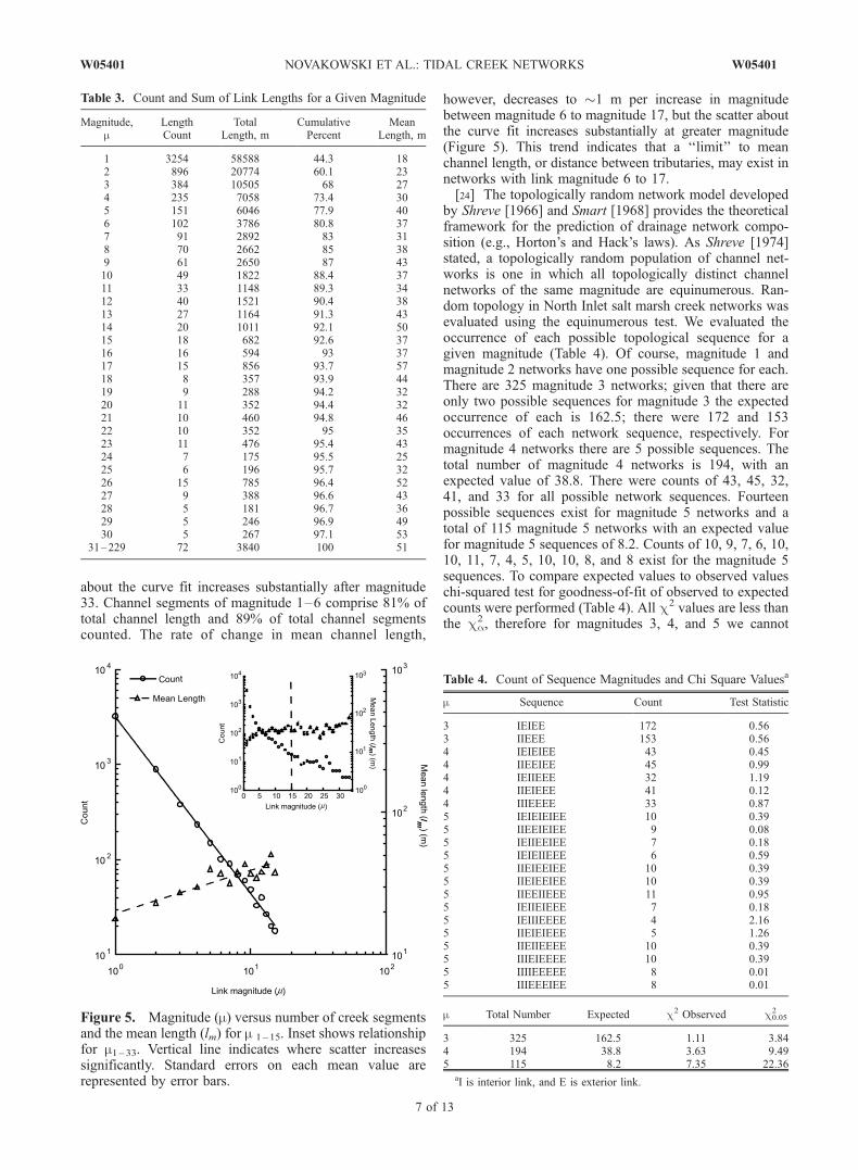
about the curve fit increases substantially after magnitude33. Channel segments of magnitude 1–6 comprise 81% oftotal channel length and 89% of total channel segmentscounted. The rate of change in mean channel length,

however, decreases to �1 m per increase in magnitudebetween magnitude 6 to magnitude 17, but the scatter aboutthe curve fit increases substantially at greater magnitude(Figure 5). This trend indicates that a ‘‘limit’’ to meanchannel length, or distance between tributaries, may exist innetworks with link magnitude 6 to 17.[24] The topologically random network model developed

by Shreve [1966] and Smart [1968] provides the theoreticalframework for the prediction of drainage network compo-sition (e.g., Horton’s and Hack’s laws). As Shreve [1974]stated, a topologically random population of channel net-works is one in which all topologically distinct channelnetworks of the same magnitude are equinumerous. Ran-dom topology in North Inlet salt marsh creek networks wasevaluated using the equinumerous test. We evaluated theoccurrence of each possible topological sequence for agiven magnitude (Table 4). Of course, magnitude 1 andmagnitude 2 networks have one possible sequence for each.There are 325 magnitude 3 networks; given that there areonly two possible sequences for magnitude 3 the expectedoccurrence of each is 162.5; there were 172 and 153occurrences of each network sequence, respectively. Formagnitude 4 networks there are 5 possible sequences. Thetotal number of magnitude 4 networks is 194, with anexpected value of 38.8. There were counts of 43, 45, 32,41, and 33 for all possible network sequences. Fourteenpossible sequences exist for magnitude 5 networks and atotal of 115 magnitude 5 networks with an expected valuefor magnitude 5 sequences of 8.2. Counts of 10, 9, 7, 6, 10,10, 11, 7, 4, 5, 10, 10, 8, and 8 exist for the magnitude 5sequences. To compare expected values to observed valueschi-squared test for goodness-of-fit of observed to expectedcounts were performed (Table 4). All c2 values are less thanthe ca

2 , therefore for magnitudes 3, 4, and 5 we cannot

Table 3. Count and Sum of Link Lengths for a Given Magnitude

Magnitude,m

LengthCount

TotalLength, m

CumulativePercent

MeanLength, m

1 3254 58588 44.3 182 896 20774 60.1 233 384 10505 68 274 235 7058 73.4 305 151 6046 77.9 406 102 3786 80.8 377 91 2892 83 318 70 2662 85 389 61 2650 87 4310 49 1822 88.4 3711 33 1148 89.3 3412 40 1521 90.4 3813 27 1164 91.3 4314 20 1011 92.1 5015 18 682 92.6 3716 16 594 93 3717 15 856 93.7 5718 8 357 93.9 4419 9 288 94.2 3220 11 352 94.4 3221 10 460 94.8 4622 10 352 95 3523 11 476 95.4 4324 7 175 95.5 2525 6 196 95.7 3226 15 785 96.4 5227 9 388 96.6 4328 5 181 96.7 3629 5 246 96.9 4930 5 267 97.1 53

31–229 72 3840 100 51

Table 4. Count of Sequence Magnitudes and Chi Square Valuesa

m Sequence Count Test Statistic

3 IEIEE 172 0.563 IIEEE 153 0.564 IEIEIEE 43 0.454 IIEEIEE 45 0.994 IEIIEEE 32 1.194 IIEIEEE 41 0.124 IIIEEEE 33 0.875 IEIEIEIEE 10 0.395 IIEEIEIEE 9 0.085 IEIIEEIEE 7 0.185 IEIEIIEEE 6 0.595 IIEIEEIEE 10 0.395 IIEIEEIEE 10 0.395 IIEEIIEEE 11 0.955 IEIIEIEEE 7 0.185 IEIIIEEEE 4 2.165 IIEIEIEEE 5 1.265 IIEIIEEEE 10 0.395 IIIEIEEEE 10 0.395 IIIIEEEEE 8 0.015 IIIEEEIEE 8 0.01

m Total Number Expected c2 Observed c0.052

3 325 162.5 1.11 3.844 194 38.8 3.63 9.495 115 8.2 7.35 22.36

aI is interior link, and E is exterior link.

Figure 5. Magnitude (m) versus number of creek segmentsand the mean length (lm) for m 1–15. Inset shows relationshipfor m1–33. Vertical line indicates where scatter increasessignificantly. Standard errors on each mean value arerepresented by error bars.

W05401 NOVAKOWSKI ET AL.: TIDAL CREEK NETWORKS

7 of 13

W05401

reject the hypothesis that marsh creek networks are topo-logically random.

4.3. Hack’s Law

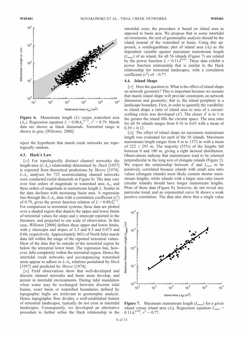
[25] For topologically distinct channel networks thelength-area (L-Aw) relationship determined by Hack [1957]is expected from theoretical predictions by Shreve [1974].L-Aw analyses for 725 nonreticulating channel networkswere conducted (solid diamonds in Figure 6). The data varyover four orders of magnitude in watershed area Aw, andthree orders of magnitude in mainstream length L. Scatter inthe data declines with increasing basin area. A regressionline through the L-Aw data with a correlation coefficient (r2)of 0.79, gives the power function relation of L = 0.08Aw

0.73.For comparison to terrestrial systems, these data are plottedover a shaded region that depicts the upper and lower limitsof terrestrial values for slope and y intercept reported in theliterature, and projected to our scale of observation. In thiscase, Willemin [2000] defines these upper and lower limits,with y intercepts and slopes of 2.3 and 0.5 and 0.073 and0.60, respectively. Approximately 86% of North Inlet marshdata fall within the range of the reported terrestrial values.Most of the data that lie outside of the terrestrial region liebelow the terrestrial lower limit. The regression line, how-ever, falls completely within the terrestrial region. Hence theintertidal creek networks and accompanying watershedareas appear to adhere to L-Aw relations postulated by Hack[1957] and predicted by Shreve [1974].[26] Field observations show that well-developed and

discrete channel networks and basin areas develop, andpersist in intertidal environments. During tidal inundationwhen water may be exchanged between discrete tidalbasins, exact basin or watershed boundaries defined bytopographic highs are irrelevant to geomorphic analysis.Hence topographic flow divides, a well-established featureof terrestrial landscapes, typically do not exist in intertidallandscapes. Consequently, we developed an alternativeprocedure to further refine the Hack relationship in the

intertidal zone; the procedure is based on island area asopposed to basin area. We propose that in some intertidalenvironments, the unit of geomorphic analysis should be theisland instead of the watershed or basin. Using this ap-proach, a semilogarithmic plot of island area (AI) as thedependent variable against maximum mainstream length(Lmax) of an island, for all 56 islands (Figure 7) are relatedby the power function L = 0.11A0.65. These data exhibit apower function relationship that is similar to the Hackrelationship for terrestrial landscapes, with a correlationcoefficient (r2) of �0.77.

4.4. Island Shape

[27] Here the question is: What is the effect of island shapeon network geometry? This is important because we assumethat marsh island shape will provide constraints on networkdimension and geometry; that is, the island periphery is alandscape boundary. First, in order to quantify the variabilityin island shape a ratio of island area to area of a circum-scribing circle was developed (A0). The closer A0 is to 1 mthe greater the island fills the circular space. The area ratiofor all 56 islands ranges from 0.16 to 0.65 with a mean of0.39 ± 0.12.[28] The effect of island shape on maximum mainstream

length was evaluated for each of the 56 islands. Maximummainstream length ranges from 8 m to 1372 m with a meanof 222 ± 293 m. The majority (55%) of the lengths fallbetween 0 and 100 m, giving a right skewed distribution.Observations indicate that mainstreams tend to be orientedperpendicular to the long axis of elongate islands (Figure 2).We expect the relationship between A0 and Lmax to bepositively correlated because islands with small area ratiovalues (elongate islands) most likely contain shorter main-stream lengths, while islands with a larger area ratio (morecircular islands) should have longer mainstream lengths.Plots of these data (Figure 8), however, do not reveal anyparticular trend, and an exponential curve fit shows a weakpositive correlation. The data also show that a single value

Figure 6. Mainstream length (L) versus watershed area(Aw). Regression equation L = 0.08Aw

0.73, r2 = 0.79. Marshdata are shown as black diamonds. Terrestrial range isshown in gray [Willemin, 2000].

Figure 7. Maximum mainstream length (Lmax) for a givenisland versus island area (AI). Regression equation Lmax =0.11AI

0.65, r2 = 0.77.

8 of 13

W05401 NOVAKOWSKI ET AL.: TIDAL CREEK NETWORKS W05401

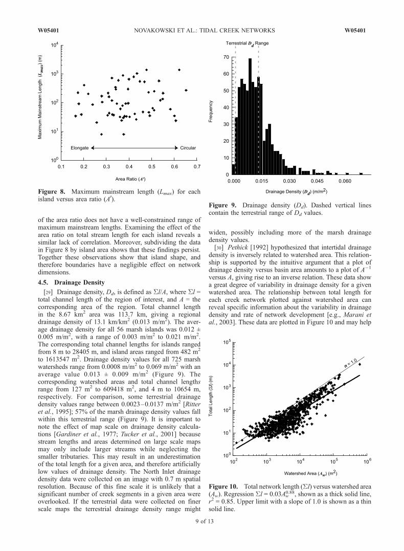
of the area ratio does not have a well-constrained range ofmaximum mainstream lengths. Examining the effect of thearea ratio on total stream length for each island reveals asimilar lack of correlation. Moreover, subdividing the datain Figure 8 by island area shows that these findings persist.Together these observations show that island shape, andtherefore boundaries have a negligible effect on networkdimensions.

4.5. Drainage Density

[29] Drainage density, Dd, is defined as Sl/A, where Sl =total channel length of the region of interest, and A = thecorresponding area of the region. Total channel lengthin the 8.67 km2 area was 113.7 km, giving a regionaldrainage density of 13.1 km/km2 (0.013 m/m2). The aver-age drainage density for all 56 marsh islands was 0.012 ±0.005 m/m2, with a range of 0.003 m/m2 to 0.021 m/m2.The corresponding total channel lengths for islands rangedfrom 8 m to 28405 m, and island areas ranged from 482 m2

to 1613547 m2. Drainage density values for all 725 marshwatersheds range from 0.0008 m/m2 to 0.069 m/m2 with anaverage value 0.013 ± 0.009 m/m2 (Figure 9). Thecorresponding watershed areas and total channel lengthsrange from 127 m2 to 609418 m2, and 4 m to 10654 m,respectively. For comparison, some terrestrial drainagedensity values range between 0.0023–0.0137 m/m2 [Ritteret al., 1995]; 57% of the marsh drainage density values fallwithin this terrestrial range (Figure 9). It is important tonote the effect of map scale on drainage density calcula-tions [Gardiner et al., 1977; Tucker et al., 2001] becausestream lengths and areas determined on large scale mapsmay only include larger streams while neglecting thesmaller tributaries. This may result in an underestimationof the total length for a given area, and therefore artificiallylow values of drainage density. The North Inlet drainagedensity data were collected on an image with 0.7 m spatialresolution. Because of this fine scale it is unlikely that asignificant number of creek segments in a given area wereoverlooked. If the terrestrial data were collected on finerscale maps the terrestrial drainage density range might

widen, possibly including more of the marsh drainagedensity values.[30] Pethick [1992] hypothesized that intertidal drainage

density is inversely related to watershed area. This relation-ship is supported by the intuitive argument that a plot ofdrainage density versus basin area amounts to a plot of A�1

versus A, giving rise to an inverse relation. These data showa great degree of variability in drainage density for a givenwatershed area. The relationship between total length foreach creek network plotted against watershed area canreveal specific information about the variability in drainagedensity and rate of network development [e.g., Marani etal., 2003]. These data are plotted in Figure 10 and may help

Figure 8. Maximum mainstream length (Lmax) for eachisland versus area ratio (A0).

Figure 9. Drainage density (Dd). Dashed vertical linescontain the terrestrial range of Dd values.

Figure 10. Total network length (Sl) versus watershed area(Aw). Regression Sl = 0.03Aw

0.88, shown as a thick solid line,r2 = 0.85. Upper limit with a slope of 1.0 is shown as a thinsolid line.

W05401 NOVAKOWSKI ET AL.: TIDAL CREEK NETWORKS

9 of 13

W05401

visualize the extent of network dissection into the marshplatform. While scatter on this plot increases as areaincreases, for basins with area greater than �2000 m2 theupper limit to the plot defines a nearly straight line with aslope of 1.0. This means that for larger basins, total channellength can be expected to increase up to a predictable lengthdetermined by a power function with a unit exponent(Figure 10). Moreover, the positive regression through thesedata gives the power function Sl = 0.03Aw

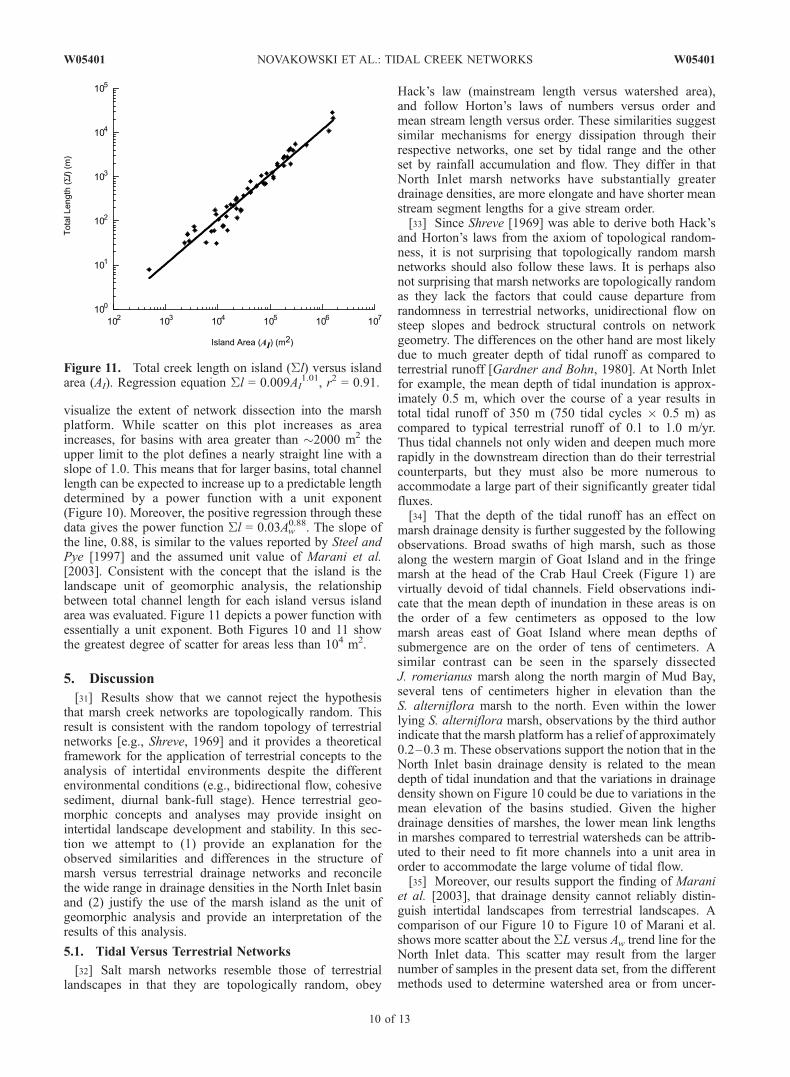
0.88. The slope ofthe line, 0.88, is similar to the values reported by Steel andPye [1997] and the assumed unit value of Marani et al.[2003]. Consistent with the concept that the island is thelandscape unit of geomorphic analysis, the relationshipbetween total channel length for each island versus islandarea was evaluated. Figure 11 depicts a power function withessentially a unit exponent. Both Figures 10 and 11 showthe greatest degree of scatter for areas less than 104 m2.

5. Discussion

[31] Results show that we cannot reject the hypothesisthat marsh creek networks are topologically random. Thisresult is consistent with the random topology of terrestrialnetworks [e.g., Shreve, 1969] and it provides a theoreticalframework for the application of terrestrial concepts to theanalysis of intertidal environments despite the differentenvironmental conditions (e.g., bidirectional flow, cohesivesediment, diurnal bank-full stage). Hence terrestrial geo-morphic concepts and analyses may provide insight onintertidal landscape development and stability. In this sec-tion we attempt to (1) provide an explanation for theobserved similarities and differences in the structure ofmarsh versus terrestrial drainage networks and reconcilethe wide range in drainage densities in the North Inlet basinand (2) justify the use of the marsh island as the unit ofgeomorphic analysis and provide an interpretation of theresults of this analysis.

5.1. Tidal Versus Terrestrial Networks

[32] Salt marsh networks resemble those of terrestriallandscapes in that they are topologically random, obey

Hack’s law (mainstream length versus watershed area),and follow Horton’s laws of numbers versus order andmean stream length versus order. These similarities suggestsimilar mechanisms for energy dissipation through theirrespective networks, one set by tidal range and the otherset by rainfall accumulation and flow. They differ in thatNorth Inlet marsh networks have substantially greaterdrainage densities, are more elongate and have shorter meanstream segment lengths for a give stream order.[33] Since Shreve [1969] was able to derive both Hack’s

and Horton’s laws from the axiom of topological random-ness, it is not surprising that topologically random marshnetworks should also follow these laws. It is perhaps alsonot surprising that marsh networks are topologically randomas they lack the factors that could cause departure fromrandomness in terrestrial networks, unidirectional flow onsteep slopes and bedrock structural controls on networkgeometry. The differences on the other hand are most likelydue to much greater depth of tidal runoff as compared toterrestrial runoff [Gardner and Bohn, 1980]. At North Inletfor example, the mean depth of tidal inundation is approx-imately 0.5 m, which over the course of a year results intotal tidal runoff of 350 m (750 tidal cycles � 0.5 m) ascompared to typical terrestrial runoff of 0.1 to 1.0 m/yr.Thus tidal channels not only widen and deepen much morerapidly in the downstream direction than do their terrestrialcounterparts, but they must also be more numerous toaccommodate a large part of their significantly greater tidalfluxes.[34] That the depth of the tidal runoff has an effect on

marsh drainage density is further suggested by the followingobservations. Broad swaths of high marsh, such as thosealong the western margin of Goat Island and in the fringemarsh at the head of the Crab Haul Creek (Figure 1) arevirtually devoid of tidal channels. Field observations indi-cate that the mean depth of inundation in these areas is onthe order of a few centimeters as opposed to the lowmarsh areas east of Goat Island where mean depths ofsubmergence are on the order of tens of centimeters. Asimilar contrast can be seen in the sparsely dissectedJ. romerianus marsh along the north margin of Mud Bay,several tens of centimeters higher in elevation than theS. alterniflora marsh to the north. Even within the lowerlying S. alterniflora marsh, observations by the third authorindicate that the marsh platform has a relief of approximately0.2–0.3 m. These observations support the notion that in theNorth Inlet basin drainage density is related to the meandepth of tidal inundation and that the variations in drainagedensity shown on Figure 10 could be due to variations in themean elevation of the basins studied. Given the higherdrainage densities of marshes, the lower mean link lengthsin marshes compared to terrestrial watersheds can be attrib-uted to their need to fit more channels into a unit area inorder to accommodate the large volume of tidal flow.[35] Moreover, our results support the finding of Marani

et al. [2003], that drainage density cannot reliably distin-guish intertidal landscapes from terrestrial landscapes. Acomparison of our Figure 10 to Figure 10 of Marani et al.shows more scatter about the SL versus Aw trend line for theNorth Inlet data. This scatter may result from the largernumber of samples in the present data set, from the differentmethods used to determine watershed area or from uncer-

Figure 11. Total creek length on island (Sl) versus islandarea (AI). Regression equation Sl = 0.009AI

1.01, r2 = 0.91.

10 of 13

W05401 NOVAKOWSKI ET AL.: TIDAL CREEK NETWORKS W05401

tainty in manual delineation of lengths. Alternatively, wespeculate that the smaller basins (102–104 m2) may haveadjusted their total creek lengths to accommodate the greaterinflux of water attributed to sea level rise. This results in thescatter of points that lie above the n = 1.0 line on Figure 10,indicating that total channel length is increasing. Moreover,the scatter in these data largely is largely below the lowerrange of values reported by Marani et al. These observationsindicate that the North Inlet intertidal watersheds are notcharacterized by a spatially uniform drainage density, unlikethe results of Marani et al. We speculate that variations indrainage density in intertidal wetlands arise from variationsin mean elevation among watersheds, and thus mainly are afunction of the tidal prism. Accordingly, greater drainagedensity should facilitate the flood and ebb of tidal waters inlower lying marsh watersheds.[36] At first glance this conclusion would seem to be at

odds with the results presented by Marani et al. [2003]whose marsh watersheds showed little variation in drainagedensity, but significant regional variation in the relationshipof total channel length to the volume of the tidal prism. Inthe Venice Lagoon, we hypothesize that the lower lyingSt. Felice basins have a larger tidal prism for a given totalchannel length than do the higher Pagliaga basins despitethe fact that the regressions of total channel length versusbasin area for the two systems are collinear and thus ofuniform drainage density (e.g., unit slope of Marani et al.’sFigure 10). We reconcile this discrepancy in the followingway: First, on the basis of our data and that of Marani et al.[2003], it appears empirically that there is an upper limit tothe total channel length that can be accommodated by agiven basin area which constrains the drainage density to amaximum value of about 0.025 m�1 (approximate y inter-cept of Figure 10 and Marani et al.’s Figure 10). Almost allof the basins in the Venice Lagoon are at or close to thislimit whereas many of the basins in the North Inlet systemfall substantially below it (Figure 10). We further hypoth-esize that it is not only total channel length that must adjustto the mean tidal prism but also total channel planform area,which is the product of total channel length by the meanchannel width. This is because ease of flow into a marshwatershed at stages above bank-full does not depend solelyon total channel length but rather on total planform channelarea. In summary, we suggest that since marsh channelnetworks are topologically random they are free to take on arange of network structures within the constraints imposedby the empirical limit on drainage density and the totalchannel area required to accommodate the tidal prism.

5.2. Salt Marsh Islands

[37] We hypothesize that island boundaries should exertsome control on the length of the networks it contains.Specifically, island shape should restrict the size of net-works present on a given island. For example, given islandsof equal area, a small area ratio, A0, (long, narrow island)should maintain a correspondingly shorter maximum chan-nel length, and a larger area ratio should support a largermaximum channel length. However, a plot of maximummainstream length (Lmax) and area ratio exhibits no generaltrend (Figure 8); hence island shape exhibits little control onmainstream length. This finding may be the result of timingof channel initiation on an island and competition for areabetween adjoining networks. Networks that begin to form at

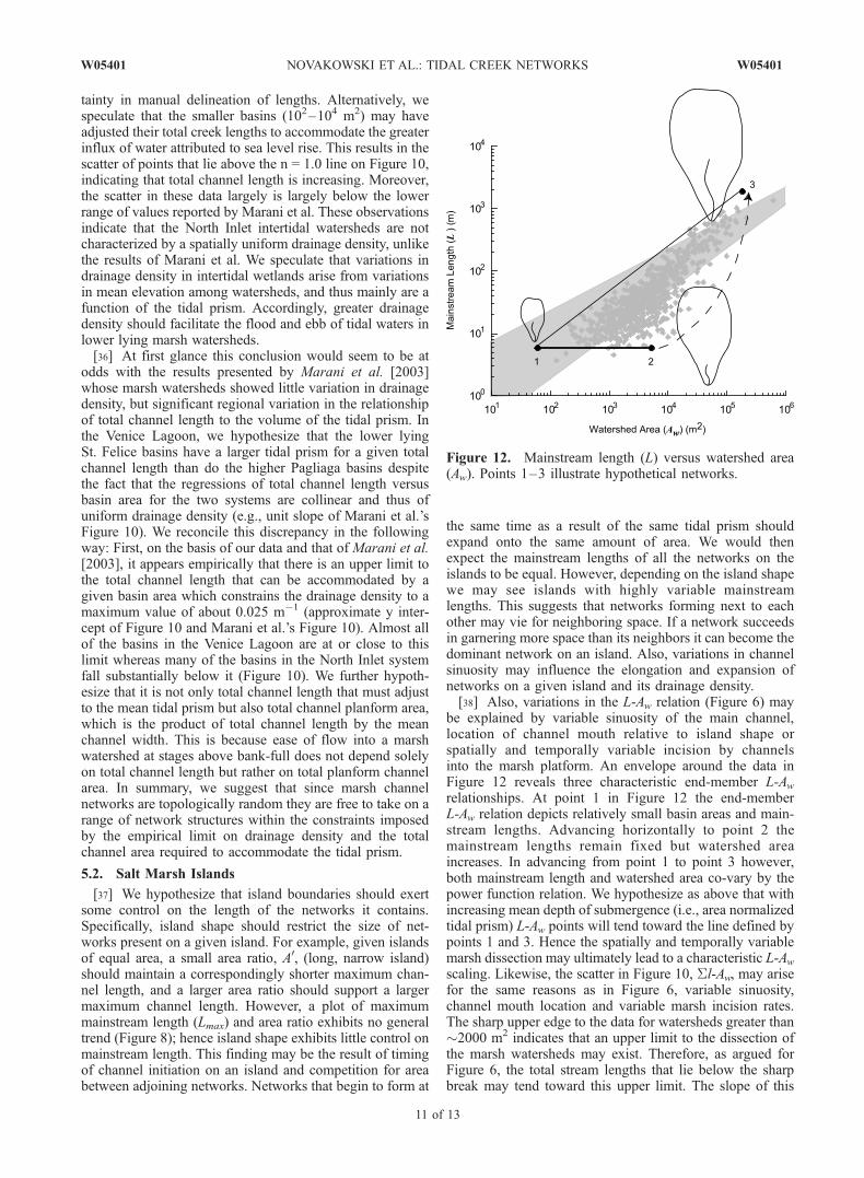
the same time as a result of the same tidal prism shouldexpand onto the same amount of area. We would thenexpect the mainstream lengths of all the networks on theislands to be equal. However, depending on the island shapewe may see islands with highly variable mainstreamlengths. This suggests that networks forming next to eachother may vie for neighboring space. If a network succeedsin garnering more space than its neighbors it can become thedominant network on an island. Also, variations in channelsinuosity may influence the elongation and expansion ofnetworks on a given island and its drainage density.[38] Also, variations in the L-Aw relation (Figure 6) may

be explained by variable sinuosity of the main channel,location of channel mouth relative to island shape orspatially and temporally variable incision by channelsinto the marsh platform. An envelope around the data inFigure 12 reveals three characteristic end-member L-Awrelationships. At point 1 in Figure 12 the end-memberL-Aw relation depicts relatively small basin areas and main-stream lengths. Advancing horizontally to point 2 themainstream lengths remain fixed but watershed areaincreases. In advancing from point 1 to point 3 however,both mainstream length and watershed area co-vary by thepower function relation. We hypothesize as above that withincreasing mean depth of submergence (i.e., area normalizedtidal prism) L-Aw points will tend toward the line defined bypoints 1 and 3. Hence the spatially and temporally variablemarsh dissection may ultimately lead to a characteristic L-Awscaling. Likewise, the scatter in Figure 10, Sl-Aw, may arisefor the same reasons as in Figure 6, variable sinuosity,channel mouth location and variable marsh incision rates.The sharp upper edge to the data for watersheds greater than�2000 m2 indicates that an upper limit to the dissection ofthe marsh watersheds may exist. Therefore, as argued forFigure 6, the total stream lengths that lie below the sharpbreak may tend toward this upper limit. The slope of this

Figure 12. Mainstream length (L) versus watershed area(Aw). Points 1–3 illustrate hypothetical networks.

W05401 NOVAKOWSKI ET AL.: TIDAL CREEK NETWORKS

11 of 13

W05401

upper limit is equal to 1.0. Marani et al. [2003] interprets aslope of 1.0 for a plot of total channel length and watershedarea as an indication that surface processes dissecting themarsh landscape are spatially uniform.[39] A similar relationship exists for total channel length

and island area. For example, the power function fit to Sl-AI

data in Figure 11 gives a slope 1.01. We extend Marani etal.’s interpretation to suggest that processes operating at theisland scale are spatially uniform or average out variationdue to depth of inundation. Given the difficulty in definingindividual watershed boundaries and corresponding water-shed areas, we propose that in some marsh landscapeswhere larger channels define marsh islands, the marshisland should be the preferred unit of landscape for geo-morphic analysis. Its boundaries are well defined and easilydetected from a variety of remote sensing techniques.Therefore we may no longer need to define watershed areasin marsh environments using flow divide models.[40] Finally, analyses and geomorphic parameterizations

presented here provide a framework for assessing networkfeatures and comparison of these geomorphic indices tothose developed in a relatively undisturbed marsh environ-ment. Hence this work may help establish quantifiableindicators of salt marsh disturbance.

6. Conclusions

[41] The topologically random network model [Shreve,1966; Smart, 1968] provides a theoretical framework for theexplanation and prediction of drainage network composition.Results show that we cannot reject the hypothesis that NorthInlet salt marsh creek networks are topologically random.This finding indicates that terrestrial concepts for analyzingchannel network geometry may apply to the intertidal zone.Hortonian analyses show differences in the slopes betweenterrestrial and marsh networks indicating that terrestrialnetwork extension may be much slower than marsh exten-sion. This idea is supported by the magnitude and meansegment length data showing that a limit to channel segmentlength may exist for marsh networks. Length-area analysesshow that marsh networks are more elongate than terrestrialnetworks, and relations between total stream length andwatershed area and island area suggest that networks expanduntil they reach a total network length maximum. Thismaximum value is set by the observed unit gradient betweentotal stream length and basin area and it indicates thatnetwork growth rates for islands may be uniform, while ratesfor watersheds tend toward a uniform growth rate.[42] Because of the complexity of defining individual

watershed boundaries and corresponding watershed area inthe intertidal salt marsh, we propose that the marsh islandshould be the preferred unit of landscape for geomorphicanalysis. Its boundaries are well defined and easily detectedfrom a variety of remote sensing techniques and it precludesthe arduous and sometimes arbitrary task of defining water-shed or basin area.

[43] Acknowledgments. This research was funded by the NOAANERRS Graduate Fellowship Program, NSF grant EAR 02-29358 andEPA grant R-828677. John Jensen and Steven Schill provided the ADARimagery. John Grego provided insight on random probability theory.Sergio Fagherazzi, Jonas Almeida, and Alan James provided insightfulcomments.

ReferencesAllen, J., and K. Pye (1992), Saltmarshes: Morphodynamics, Conservationand Engineering Significance, Cambridge Univ. Press, New York.

Brush, L. (1961), Drainage basins, channels, and flow characteristics ofselected streams in central Pennsylvania, U.S. Geol. Surv. Prof. Pap.,282-F, 161–181.

Cleveringa, J., and A. Oost (1999), The fractal geometry of tidal-channelsystems in the Dutch Wadden Sea, Geol. Mijnbouw, 78(1), 21–30.

Collins, L., J. Collins, and L. Leopold (1987), Geomorphic processes of anestuarine marsh: Preliminary results and hypotheses, in InternationalGeomorphology: Proceedings of the First International Conference onGeomorphology, part I, edited by V. Gardiner, pp. 1049–1072, JohnWiley, Hoboken, N. J.

Fagherazzi, S., and D. Furbish (2001), On the shape and widening of saltmarsh creeks, J. Geophys. Res., 106, 991–1003.

Fagherazzi, S., A. Bortoluzzi, W. Dietrich, A. Adami, A. Lanzoni,M. Marani, and A. Rinaldo (1999), Automatic network extraction andpreliminary scaling features from digital terrain maps, Water Resour.Res., 35(12), 3891–3904.

Gardiner, V., K. Gregory, and D. Walling (1977), Further notes on thedrainage density-basin area relationship, Area, 9, 117–121.

Gardner, L., and M. Bohn (1980), Geomorphic and hydraulic evolution oftidal creeks on a subsiding beach ridge plain, North Inlet, South Carolina,Mar. Geol., 34, M91–M97.

Gardner, L. R., and W. Kitchens (1978), Sediment and chemical exchangesbetween salt marshes and coastal waters, in Transport Processes inEstuarine Environments, edited by B. Kjerfve, Univ. of S. C. Press,Columbia.

Gardner, L., and D. Porter (2000), Stratigraphy and geologic history of asoutheastern salt marsh basin, North Inlet, South Carolina, USA, Wet-lands Ecol. Manage., 9(5), 1–15.

Gardner, L., L. Thombs, D. Edwards, and D. Nelson (1989), Time seriesanalyses of suspended sediment concentrations at North Inlet, SouthCarolina, Estuaries, 12(4), 211–221.

Geyl, W. (1976), Tidal neomorphs, Z. Geomorphol., 20(3), 308–330.Goni, M. A., and K. A. Thomas (2000), Sources and transformations oforganic matter in surface soils and sediments from a tidal estuary (NorthInlet, South Carolina, USA), Estuaries, 23(4), 548–564.

Hack, J. (1957), Studies of longitudinal stream profiles in Virginia andMaryland, U.S. Geol. Surv. Prof. Pap., 294-B.

Horton, R. (1945), Erosional development of streams and their drainagebasins: Hydrophysical approach to quantitative morphology, Geol. Soc.Am. Bull., 56, 273–370.

Jensen, J. (2000), Remote Sensing of the Environment: An Earth ResourceApproach, 544 pp., Prentice-Hall, Old Tappan, N. J.

Jensen, J., G. Olsen, S. Schill, D. Porter, and J. Morris (2002), Remotesensing of biomass, leaf-area-index, and chlorophyll a and b content inthe ACE Basin National Estuarine Research Reserve using sub-meterdigital camera imagery, Geocarto Int., 17(3), 25–34.

Kirchner, J. (1993), Statistical inevitability of Horton’s laws and theapparent randomness of stream channel networks, Geology, 21, 591–599.

Knighton, A., C. Woodroffe, and K. Mills (1992), The evolution of tidalcreek networks, Mary River, northern Australia, Earth Surf. ProcessesLandforms, 17, 167–190.

Langbein, W. (1963), The hydraulic geometry of a shallow estuary, Int.Assoc. Sci. Hydrol., 8, 84–94.

Leonard, L. (1997), Controls of sediment transport and deposition in anincised mainland marsh basin, southeastern North Carolina, Wetlands,17(2), 263–274.

Marani, M., E. Belluco, A. D’Alpaos, A. Defina, S. Lanzoni, and A. Rinaldo(2003), On the drainage density of tidal networks, Water Resour. Res.,39(2), 1040, doi:10.1029/2001WR001051.

Myrick, R., and L. B. Leopold (1963), Hydraulic geometry of a small tidalestuary, U.S. Geol. Surv. Prof. Pap., 422-B.

Pestrong, R. (1965), The development of drainage patterns on tidalmarshes, Ph.D. thesis, Stanford Univ., Stanford, Calif.

Pethick, J. (1980), Velocity surges and asymmetry in tidal channels,Estuarine Coastal Mar. Sci., 11, 331–345.

Pethick, J. (1992), Saltmarsh geomorphology, in Saltmarsh Geomorphology:Morphodynamics, Conservation, and Engineering Significance, edited byJ. Allen and K. Pye, Cambridge Univ. Press, New York.

Ragotzkie, R. (1959), Drainage pattern in salt marshes, in Proceedings ofthe Salt Marsh Conference, pp. 22–28, Mar. Inst., Univ. of Ga., Atlanta.

Redfield, A. (1972), Development of a New England salt marsh, Ecol.Monogr., 24(2), 201–237.

12 of 13

W05401 NOVAKOWSKI ET AL.: TIDAL CREEK NETWORKS W05401

Rinaldo, A., S. Fagherazzi, A. Lanzoni, M. Marani, and W. Dietrich(1999a), Tidal networks: 2. Watershed delineation and comparative net-work morphology, Water Resour. Res., 35(12), 3905–3917.

Rinaldo, A., S. Fagherazzi, A. Lanzoni, M. Marani, and W. Dietrich(1999b), Tidal networks: 3. Landscape forming discharges and studiesin empirical geomorphic relationships, Water Resour. Res., 35(12),3919–3929.

Ritter, D., R. Kochel, and J. Miller (1995), Process Geomorphology,545 pp., Wm. C. Brown, Dubuque.

Sharma, P., L. Gardner, W. Moore, and M. Bollinger (1987), Sedimentationand bioturbation in a salt marsh as revealed by 210Pb, 137Cs, and 7Bestudies, Limnol. Oceanogr., 32(2), 313–326.

Shreve, R. (1966), Statistical law of stream numbers, J. Geol., 74(1), 17–37.Shreve, R. (1969), Stream lengths and basin areas in topologically randomchannel networks, J. Geol., 77(4), 397–414.

Shreve, R. (1974), Variation of mainstream length with basin area in rivernetworks, Water Resour. Res., 10(6), 1167–1177.

Smart, J. (1968), Mean stream numbers and branching ratios for topologi-cally random channel networks, Bull. Int. Assoc. Sci. Hydrol., 13, 61–64.

Steel, T., and K. Pye (1997), The development of saltmarsh tidal creeknetworks: Evidence from the UK, paper presented at Canadian CoastalConference, Can. Coastal Sci. and Eng. Assoc., Guelph, Ontario.

Torres, R., M. Mwamba, and M. Goni (2003), Properties of intertidal marshsediment mobilized by rainfall, Limnol. Oceanogr., 48(3), 1245–1253.

Tucker, G., F. Catani, A. Rinaldo, and R. Bras (2001), Statistical analysis ofdrainage density from digital terrain data, Geomorphology, 36, 187–202.

Valdes, J., Y. Fiallo, and I. Rodriguez-Iturbe (1979), A rainfall-runoff anal-ysis of the geomorphologic IUH, Water Resour. Res., 15(6), 1421–1434.

Vogel, R. L., B. Kjerfve, and L. R. Gardner (1996), Inorganic sedimentbudget for the North Inlet Salt Marsh, South Carolina, USA, MangrovesSalt Marshes, 1(1), 23–25.

Wadsworth, J. (1980), Geomorphic characteristics of tidal drainage net-works in the Duplin River system, Sapelo Island Georgia, Ph.D. Thesis,Univ. of Ga., Atlanta.

Willemin, J. (2000), Hack’s law: Sinuosity, convexity, elongation, WaterResour. Res., 36(11), 3365–3374.

Wright, L., J. Coleman, and B. Thom (1973), Processes of channel devel-opment in a high-tide range environment: Cambridge Gulf-Ord RiverDelta, Western Australia, J. Geol., 81, 15–41.

Zeff, M. (1999), Salt marsh tidal channel morphometry: Applications forwetland creation and restoration, Restoration Ecol., 7(2), 205–211.

����������������������������L. R. Gardner, K. I. Novakowski, R. Torres, and G. Voulgaris,

Department of Geological Sciences, University of South Carolina, 701Sumter Avenue, EWS 617, Columbia, SC 29208, USA. (kinovakowski@yahoo.com; torres@geol.sc.edu)

W05401 NOVAKOWSKI ET AL.: TIDAL CREEK NETWORKS

13 of 13

W05401

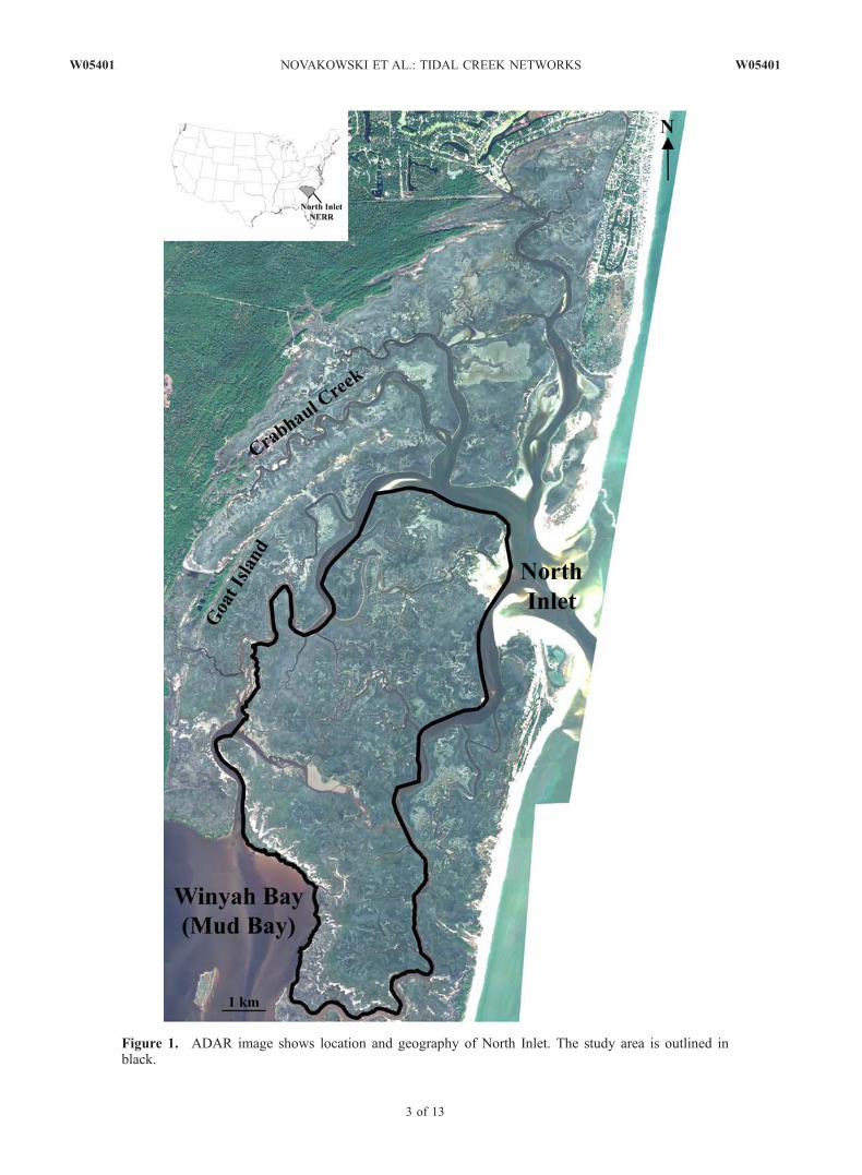
Figure 1. ADAR image shows location and geography of North Inlet. The study area is outlined inblack.

3 of 13

W05401 NOVAKOWSKI ET AL.: TIDAL CREEK NETWORKS W05401