Geometric modeling of subcellular structures, organelles and

multiprotein complexes

Xin Feng 1, Kelin Xia 2, Yiying Tong1∗, and Guo Wei Wei2,3†1Department of Computer Science and Engineering

Michigan State University, MI 48824, USA2Department of Mathematics

Michigan State University, MI 48824, USA3Department of Electrical and Computer Engineering

Michigan State University, MI 48824, USA

October 10, 2012

Abstract

Recently, the structure, function, stability and dynamics of subcellular structures, organelles andmultiprotein complexes have emerged as a leading interest in structural biology. Geometric model-ing not only provides visualizations of shapes for large biomolecular complexes, but also fills the gapbetween structural information and theoretical modeling, and enables the understanding of function,stability and dynamics. This paper introduces a suite of computational tools for volumetric dataprocessing, information extraction, surface mesh rendering, geometric measurement, and curvatureestimation of biomolecular complexes. Particular emphasis is given to the modeling of cryo-electronmicroscopy (cryo-EM) data. Lagrangian-triangle meshes are employed for the surface presentation.Based on this representation, algorithms are developed for surface area and volume calculation, andcurvature estimation. Methods for volumetric meshing have also been presented. Since the technolog-ical development in computer science and mathematics has led to multiple choices at each stage of thegeometric modeling, we discuss the rationales in the design and selection of various algorithms. Analyt-ical models are designed to test the computational accuracy and convergence of proposed algorithms.Finally, we select a set of six cryo-EM data representing typical subcellular complexes to demonstratethe efficacy of the proposed algorithms in handling biomolecular surfaces, and explore their capabilityof geometric characterization of binding targets. This paper offers a comprehensive protocol for thegeometric modeling of subcellular structures, organelles and multiprotein complexes.

Key words: Geometric modeling, Laplace-Beltrami operator, High order geometric PDEs, Surfacemeshing, Gaussian curvature, Mean curvature.

∗Corresponding author. E-mail:ytong@msu.edu†Corresponding author. E-mail:wei@math.msu.edu

1

Contents

1 Introduction 3

2 Methods 62.1 High order geometric flows . . . . . . . . . . . . . . . . . . . . . . . . . . . . . . . . . . . . . 62.2 Nonlinear PDE based high pass filters . . . . . . . . . . . . . . . . . . . . . . . . . . . . . . 72.3 Surface extraction and meshing . . . . . . . . . . . . . . . . . . . . . . . . . . . . . . . . . . 72.4 Surface areas and enclosed volumes . . . . . . . . . . . . . . . . . . . . . . . . . . . . . . . 82.5 Curvatures . . . . . . . . . . . . . . . . . . . . . . . . . . . . . . . . . . . . . . . . . . . . . 8

2.5.1 Brief introduction to the continuous theory . . . . . . . . . . . . . . . . . . . . . . . 82.5.2 Curvature estimates on triangle meshes . . . . . . . . . . . . . . . . . . . . . . . . . 10

2.6 Volumetric meshing . . . . . . . . . . . . . . . . . . . . . . . . . . . . . . . . . . . . . . . . 12

3 Results and discussion 133.1 Data denoising and Surface extraction . . . . . . . . . . . . . . . . . . . . . . . . . . . . . . 143.2 Surface mesh improvement . . . . . . . . . . . . . . . . . . . . . . . . . . . . . . . . . . . . 163.3 Areas, volumes and curvatures . . . . . . . . . . . . . . . . . . . . . . . . . . . . . . . . . . 17

3.3.1 Applications of curvature estimates to cryo-EM maps . . . . . . . . . . . . . . . . . 193.4 Volumetric meshing . . . . . . . . . . . . . . . . . . . . . . . . . . . . . . . . . . . . . . . . 20

4 Conclusion 22

2

1 Introduction

One of major features of biological sciences in the 21st century is their transition from an empirical,qualitative and phenomenological discipline to a comprehensive, quantitative and predictive one. Indeed,theoretical description, mathematical modeling and computer simulation of biological systems have madeenormous contribution to the present understanding of biological sciences. The material basis and funda-mental underpinning of modern biological sciences are biological macromolecules, especially proteins andnucleic acids, which coil into specific three-dimensional (3D) shapes and are able to carry out most of thefunctions of cells. The goal of theoretical description, mathematical modeling and computer simulation isto understand the structure, function, dynamics and transport of biological macromolecules. A prerequi-site to theoretical description, mathematical modeling and computer simulation of the structure, function,dynamics and transport of biological macromolecules is the geometric modeling based on their 3D shapes.In addition to straightforward geometric visualization, geometric modeling bridges the gap between imag-ing and mathematical modeling such that the structural information can be integrated into mathematicalmodels.

Macromolecular 3D shapes can be indirectly obtained from a number of experimental means, includingmacromolecular X-ray crystallography, nuclear magnetic resonance (NMR), electron paramagnetic res-onance (EPR), cryo-electron microscopy (cryo-EM), multiangle light scattering, confocal laser-scanningmicroscopy, small angle scattering, ultra fast laser spectroscopy, etc. The main workhorses for singlemacromolecules are crystallography and NMR. The advanced X-ray crystallography technology is able toprovide decisive structural information at Armstrong and sub-Armstrong resolutions, while NMR exper-iments often offer structural information under physiological conditions. Both X-ray crystallography andNMR are technologically relatively well developed, except for their applications in special tasks, such asthe crystallization of membrane proteins. However, these approaches are not suitable for proteasomes,subcellular structures, organelles, cells and tissues. Their study has become one of the major new trendsin structural biology. Currently, one of the most powerful tools for subcellular structures, organelles andlarge multiprotein complexes is cryo-EM.

Cryo-EM, or electron cryomicroscopy, is an increasingly popular transmission electron microscopy (EM)whose sample is bombarded by electron beams at cryogenic temperatures to improve the signal to noiseratio (SNR). Its working principle is based on the projection (thin film) specimen scans collected from manydifferent directions around one or two axes, and the creation of 3D images by using the Radon transform.Cryo-EM allows the imaging of specimens in their native environment and is capable of providing 3Dmapping of entire cellular proteomes together with their detailed interactions at a nanometer resolution[48, 54, 40, 69].

Since most biological specimens are extremely radiation sensitive, they can only sustain the illuminationof a limited electron dose. As a result, cryo-EM images are inevitably of low SNR and lead to limitedresolutions [73]. In practice, cryo-EM maps often do not contain enough information to offer unambiguousatomic-scale structural reconstruction of biological specimens. Additional information obtained from othertechniques, such as crystallography, NMR and computer simulation, is utilized to interpret the cryo-EM maps. However, the resolution of cryo-EM maps has been improved dramatically in the past fewyears, thanks to the technical advances in experimental hardware, noise reduction and image segmentationtechniques. By further taking the advantage of symmetric averaging, many cryo-EM based virus structureshave already achieved a resolution that can be interpreted in terms of an atomic model. Therefore, it is timeto utilize cryo-EM images for molecular and atomic scale mathematical modeling and computer simulationof subcellular structures, organelles and large multiprotein complexes.

Most 3D imaging data obtained from cryo-EM and many other tomographic modalities are currentlypresented in a digital format, as a volumetric density distribution, where each Cartesian grid point isassigned with a scalar value associated with the local electron scattering power. For the purpose of vi-sualization, one needs to convert them into images in the form of a series of 2D images, rendering of the3D shapes generated by isosurface extraction, or direct volumetric rendering. For the purpose of geomet-ric analysis, structural features in the complex settings of cellular landscapes are further characterized interms of surface areas, surface enclosed volumes, and Gaussian and mean curvatures. For the purpose

3

of mathematical modeling and computation, the resulting 3D geometric shape is to be further describedin either the Lagrangian representation or the Eulerian representation. The Lagrangian representation isa basis for the Lagrangian formulation of the biological evolution, in which surface elements are directlyevolved according to a governing equation or a set of rules [14, 91]. Similarly, the Eulerian representationfacilitates the Eulerian formulation of the biological dynamics, in which the biological shape is embeddedin a hypersurface function, or a level set function, and such a function is then evolved under prescribedphysical and/or biological principles [4, 13, 12]. Both Lagrangian and Eulerian approaches have their ownpros and cons, and are very useful in mathematical modeling and computation. In the present work, wefocus our studies on the Lagrangian representation of 3D imaging data.

Currently, the SNR of 3D imaging data for subcellular structures, organelles and large multiproteincomplexes is typically in the neighborhood of 0.01 [73]. To make the situation worse, the image contrast,which depends on the difference between electron scattering cross sections of cellular components, is alsovery low in most biological systems. Consequently, appropriate noise reduction is an indispensable processin the structure reconstruction from 3D imaging data. To improve the SNR and image contrast of cryo-EMdata, researchers have employed a wide variety of denoising schemes, including wavelet transform techniques[66], nonlinear anisotropic diffusions [26, 23] or Beltrami flow [22], bilateral filter [70, 33, 52], and iterativemedian filtering [72]. Despite much effort, noise-reduction of cryo-EM data remains a challenging task andis far from adequate, due to the extremely low SNR and other technical complications [73]. Innovativemathematical approaches are necessary to further tackle this problem.

Geometric flows, in which the flow motion is governed or influenced by geometric properties, such ascurvatures, have become an established approach to image analysis and surface generation in the past fewyears. Particularly, mean curvature flows have been a popular subject in applied mathematics for imageanalysis, material design [64, 49, 61] and surface processing [3, 93]. The first use of partial differentialequations (PDEs) for image analysis dates back to 1983 [86]. Witkin noticed that the evolution of animage under a diffusion operator is formally equivalent to the standard Gaussian low-pass filter for imagedenoising [86]. Perona and Malik introduced an anisotropic diffusion equation [53] to protect image edgesduring the diffusion process. The Perona-Malik equation stimulated much interest in applied mathematics[53, 65, 80, 11, 82]. Over the past two decades, many related mathematical techniques, such as the levelset formalism devised by Osher and Sethian [51, 61], Mumford-Shah variational functional [47], and thetotal variation (TV) minimization [55], have been widely used for image analysis [6, 9, 50, 57, 58].

To improve the efficiency of noise removing, Wei introduced the first family of arbitrarily high ordernonlinear PDEs for image denoising and restoration in 1999 [80]. Many fourth-order evolution equationswere introduced in the literature for image analysis [11, 88, 68, 43, 30]. These equations were proposedeither as a high-order generalization of the Perona-Malik equation [80, 2] or as an extension of the TVformulation [11, 88, 68, 43]. The essential assumption in these high order evolution equations is thathigh-order diffusion operators are able to remove high frequency components more efficiently. High ordergeometric PDEs have been widely applied to image and surface analysis [10, 80, 11, 88, 68, 30, 43, 31, 2].Due to the stiffness of high order nonlinear PDEs, computational techniques for solving higher ordergeometric PDEs are of great importantance. For instance, alternating direction implicit (ADI) schemesare developed in the literature for integrating high order nonlinear PDEs [85, 2].

delete some material hereImage processing PDEs of the Perona-Malik type and total variation type are mostly designed to

function as nonlinear low-pass filters. In 2002, Wei and Jia [82] introduced coupled nonlinear PDEs tobehave as high-pass filters. These coupled nonlinear PDEs are demonstrated for image edge detection.The essential idea behind these PDE based high-pass filters is that when two Perona-Malik type of PDEsevolve at dramatically different speeds, the difference of their solutions gives rise to image edges. Thisfollows from the fact that the difference between an all-pass filter (i.e., identity operator) and a low-passone is a high-pass filter [82]. The speeds of evolution in these equations are controlled by the appropriateselection of the diffusion coefficients. These PDE-based edge detectors have been shown to work extremelywell for images with a large amount of textures [67, 82]. Most recently, the PDE transform is introducedfor functional mode decomposition, [77, 76, 78] based on arbitrarily high order PDE high-pass filters. Such

4

an approach has significantly extended the utility of PDEs for image, surface and data analysis. Similar towavelet transform, the PDE transform has controllable time-frequency location and perfect reconstruction.The PDE transform has found its success in molecular surface generation of proteins [95].

The use of curvature controlled PDEs for biomolecular surface construction was initiated in 2005 [83].Atomic coordinate information of a protein is embedded in 3D Eulerian grids to undergo geometric flowevolution before the protein surface is extracted via the marching cubes method from a level-set type ofhypersurface function. This approach was combined with a variational procedure to generate the firstvariational biomolecular surface model, the minimal molecular surface, for proteins [3, 4]. Molecularinteractions were further incorporated in this approach to develop potential and curvature driven geometricflows for the construction of biomolecular surfaces [2]. Recently, many variational multiscale models havebeen introduced based on the geometric-flow separation of solvent and solute domains [81, 13, 12, 94].

After the surface construction, a further issue in geometric modeling is the surface and volumet-ric (i.e., boundary and interior) meshing [58, 19, 44]. There are a wide variety of methods that canbe used for this purpose. Numerous elegant methods such as, the probabilistic methods for CentroidalVoronoi Tessellations[20, 34], the Optimal Delaunay Triangulation and graph cut based variational surfacereconstruction[74], and other surface remeshing enhancement methods and technologies [59, 56, 58, 79, 27],have been developed for surface reconstruction or surface remeshing during the past two decades. In general,high quality triangle surface meshes must be low-noise, low memory cost, near 60◦ for majority of elementangles and aligned with the physical features. Yu et al. discussed the use of adaptive feature-preservingmethods for biomolecular surface meshing [91, 92]. They used the constrained Delaunay triangulationimplemented in TetGen [63] for volumetric meshing [91].

Curvature is a measure of how much a line deviates from being straight or flat in case of a surface[37]. Curvature has been used to analyze the stereospecificity of molecular surfaces [15]. The essentialidea is that geometries of binding partners are locally complementary to each other at the binding site(s).Curvatures are also used as a geometric descriptor to characterize the shape of known protein bindingsites so as to identify matching site(s) in other proteins and ligands. However, in real cases, the effectof stereospecificity may be offset by hydrogen bond, polarization, electrostatics, solvation and allostericmodulation.

The objective of the present work is to explore the efficient computational methods for the geometricmodeling of subcellular structures, organelles and large multiprotein complexes. Specifically, we study thereconstruction of biological structures from noisy 3D imaging data, examine the geometric representationof complex biological shapes, provide accurate calculation of surface areas and surface enclosed volumes,and investigate the computational algorithm and surface mapping of Gaussian and mean curvatures ofmacromolecules. Most geometric modeling is carried out in the Lagrangian representation with trianglemeshes on the surface.

The rest of this paper is organized as follows. Section 2 is devoted to computational methods andnumerical algorithms for geometric modeling. We give a brief description of high order geometric PDEsand nonlinear PDE based high-pass filters. Different surface extraction schemes are discussed. Numericalalgorithms for calculating surface areas and surface enclosed volumes are given in the Lagrangian repre-sentation. We introduce the state of the art techniques for volumetric meshing of subcellular structures,organelles and large multiprotein complexes. Efficient schemes for computing Gaussian and mean curva-tures are provided. In Section 3, we carry out extensive numerical experiments to validate the proposedmethods, algorithms, and schemes. We design analytical cases to test accuracy and convergent order ofthe proposed algorithms for area, volume and curvature calculations. Second order convergence is foundin these schemes. Finally, we apply the proposed methods to six biomolecular examples. Our resultsdemonstrate the usefulness, robustness and efficiency of the proposed approaches. This paper ends with aconclusion in Section 4.

5

2 Methods

This section provides a variety of mathematical and computational methods for geometric modeling. Thegoal here is to introduce a repertoire of appropriate computational tools for the applications involvingvolumetric data and the shapes defined in cryo-EM datasets.

2.1 High order geometric flows

Geometric flows, such as the Laplace-Beltrami flow, play a significant role in image analysis. An importantaspect in the geometric flow development is the use of high order geometric PDEs for image processingor surface analysis. Willmore flow, proposed in 1920s, is a fourth order geometric PDE which locallyminimizes the difference between two principal curvatures (see detailed description on principal curvaturesin Section 2.5.1). Therefore, the Willmore flow prefers spherical shapes, which may be undesirable ingeneral applications. Motivated by the hyperdiffusion in the pattern formation in alloys, glasses, polymer,combustion, and biological systems, one of the first family of arbitrarily high order geometric PDEs wasintroduced for edge-preserving image restoration in 1999, using Fick’s law [80]

∂u(r, t)

∂t= −

∑q

∇ · jq + e(u(r, t), |∇u(r, t)|, t), q = 0, 1, 2, · · · (1)

where the nonlinear hyperflux is given by

jq = −dq(u(r, t), |∇u(r, t)|, t)∇∇2qu(r, t), q = 0, 1, 2, · · · (2)

where r ∈ Rn, ∇ = ∂∂r , u(r, t) is the processed image function, dq(u(r, t), |∇u(r, t)|, t) are edge sensitive

diffusion coefficients and e(u(r, t), |∇u(r, t)|, t) is a nonlinear operator. Equation (1) is subject to theinitial image data u(r, 0) = X(r) and appropriate boundary conditions. The essential idea of Equation (1)is to accelerate the noise removal in the Perona-Malik equation [53] by higher order derivatives, which ismore efficient in noise dissipation. As a generalization of the Perona-Malik equation, the hyperdiffusioncoefficients dq(u, |∇u|, t) in Eq. (2) can also be chosen as the Gaussian form

dq(u(r, t), |∇u(r, t)|, t) = dq0 exp

[−|∇u|

2

2σ2q

], (3)

where the values of constant dq0 depend on the noise level, and σ0 and σ1 were chosen as the local statisticalvariance of u and ∇u

σ2q (r) = |∇qu−∇qu|2 (q = 0, 1). (4)

The notation Y (r) above denotes the local average of Y (r) centered at position r. The measure based onthe local statistical variance is important for discriminating image features from noise. As a result, onecan bypass the image preprocessing, i.e., the convolution of the noise image with a smooth mask in theapplication of the PDE operator to noisy images. High order geometric PDEs have found many practicalapplications [80, 43, 29, 28]. Arbitrarily high order geometric PDEs are modified for molecular surfaceformation and evolution [2]

∂S

∂t= (−1)q

√g(|∇∇2qS|)∇ ·

(∇(∇2qS)√g(|∇∇2qS|)

)+ P (S, |∇S|), (5)

where S is the hypersurface function, g(|∇∇2qS|) = 1+ |∇∇2qS|2 is the generalized Gram determinant andP is a generalized potential term, including microscopic interactions in biomolecular surface construction.When q = 0 and P = 0, Eq. (5) recovers the mean curvature flow used in our earlier construction ofminimal molecular surfaces [4]. It reproduces the surface diffusion flow [2] when q = 1 and P = 0. Ithas been shown that surface generated with the fourth order geometric PDE demonstrates a morphologydistinguished from that obtained with the mean curvature flow or the Laplace-Beltrami flow [2].

6

2.2 Nonlinear PDE based high pass filters

Unfortunately, the studies of geometric flows have been essentially limited to the construction of nonlinearPDE based low-pass filters. From the point of view of image and signal processing, low-pass filtering is justone specific type of operations and other filters, such as high-pass filters and band-pass filters are equallyimportant. An exception is the nonlinear PDE based high-pass filters introduced by Wei and Jia [82] forimage edge detection in 2002,

ut(r, t) = F1(u,∇u,∇2u, . . .) + εu(v − u) (6)

vt(r, t) = F2(v,∇v,∇2v, . . .) + εv(u− v) (7)

where u(r, t) and v(r, t) are scalar fields, εu and εv are coupling strengths. Here F1 and F2 are generalnonlinear diffusion operators, and can be chosen as the Perona-Malik operator F1 = ∇ · d1(|∇u|)∇ andF2 = ∇ · d2(|∇v|)∇. The initial values for both nonlinear evolution equations are chosen to be the sameimage, i.e., u(r, 0) = v(r, 0) = X(r). As a nonlinear dynamic system, the time evolution of Eqs. (6) and (7)will eventually lead to a synchronization in the solution for positive nonzero coupling coefficients. For thepurpose of image processing, Eqs. (6) and (7) are designed to evolve at dramatically different time scales,for example, the coefficients d1 and d2 are chosen as the Gaussian form in Eq. (3) with d20 >> d10 ≥ 0.After finite time evolution, the image edges are obtained as the difference [82]

w(r, t) = u(r, t)− v(r, t). (8)

It was shown that Eq. (8) behaves like a band-pass filter when d20 >> d10 ∼ 0. The essence of this approachis that when two coupled evolution PDEs are evolving at dramatically different speeds, the difference oftwo low-pass PDE operators gives rise to a band-pass or high-pass filter. The coupling terms play the roleof relative fidelity, and balance the disparity of two images. It has been shown that nonlinear PDE basedhigh-pass filters work extremely well for images with a large number of textures, and outperform classicalSobel, Prewitt, and Canny operators [67, 82].

2.3 Surface extraction and meshing

Both the 3D imaging data from cryo-EM and the result of the aforementioned Eulerian geometric flowsor PDE-based nonlinear filtering are given as functions sampled on Eulerian grids. For subsequent usein finite element methods (FEMs) or Lagrangian geometry processing, which is often much more efficientthan the Eulerian representation due to better adaptivity of the irregular sampling and the reduction from3D into curved 2D representation. In most geometry processing approaches, h-refinement (more segments)is preferred over p-refinement (degree of the polynomial in each segment), since the modern computerarchitectures can handle a large number of simple objects more efficiently than a small number of complexobjects representing the same surface [8]. In the following, we use the extremal C0 case, i.e., piece-wiseflat surface meshes, the de-facto standard data structure in current geometry processing.

The conversion from 3D image data to 2D triangle mesh is often implemented by using the widely usedmarching cubes algorithm [42]. Without loss of generality, we can assume the isosurface to be extractedis the 0 level-set. The vertices can be found on edges with opposite field values on both ends. The exactlocation of the intersection of the isosurface on the edge can be easily computed based on the trilinearinterpolation approximation of the continuous underlying field, which reduces to linear interpolation alongthe edge. The mesh connectivity is then established by examining each cell and constructing triangleswith vertices on the edges of that cell by checking in a predetermined lookup table, which contains theconnectivity information of the vertices within each cell for the 256 possible sign configurations of the 8grid points of the cell. The actual lookup table is reduced to 15 cases by using symmetry. For some cases,disambiguation based on actual field values is necessary [45].

We recommend the use of marching cubes for applications that do not require well-shaped elements, asthis approach is highly parallelizable. On the other hand, for FEM and other applications with stringentrequirement on the maximum and minimum angles of each triangle, we propose to use an alternative based

7

on restricted Delaunay triangulation [7]. A sample implementation is available from the ComputationalGeometry Algorithms Library (CGAL) [17]. It distributes sample points on the surface, and then extractsan interpolating triangle mesh through the 3D triangulation of the points. These points are added iter-atively following a Delaunay refinement-like step until the sizes and shapes of the mesh triangles meetspecified criteria. Other choices include dual contouring for adaptive octree data [35, 5], and the ExtendedMarching Cubes for models with sharp features [36], which might be rare for cryo-EM datasets though.

2.4 Surface areas and enclosed volumes

Surface area and enclosed volume are crucial components in the mathematical and thermodynamical mod-eling of biomolecular systems [81, 84, 13, 14]. Given a Lagrangian mesh with piecewise flat segments, it isstraightforward to compute the surface area and enclosed volume. For surface area, one simply sums upthe area of each surface triangle,

A(S) =

∫S

1 dA =∑tl∈T|tl| =

∑tl∈T

1

2|(vk − vi)× (vj − vi)|, (9)

where S is the surface of the biomolecule, A(S) is the total surface area, and T contains all the surfacetriangles in a tessellation of S. Here tl is a triangle mesh element, with vi, vj and vk as the coordinatesof its three vertices.

To calculate the volume on the mesh, one picks an arbitrary point inside or outside the mesh, forexample, the origin, and sums up all the signed volume of the tetrahedron formed by the point and eachtriangle,

V (S) =

∫S

x · n dA =∑tl∈T

1

6((vk − vi)× (vj − vi)) · vi, (10)

where V (S) is the total volume, n is the outward surface normal at a position x on the surface S. Here thevertices of each triangle are assumed to be listed in counterclockwise order when viewed from the outsideof the surface. Even when a volumetric mesh of the inside is available, summing up the volumes of thesethin tetrahedra formed by a fixed point and boundary faces is in general much more efficient than summingup the volumes all the tetrahedra of the volumetric mesh.

2.5 Curvatures

2.5.1 Brief introduction to the continuous theory

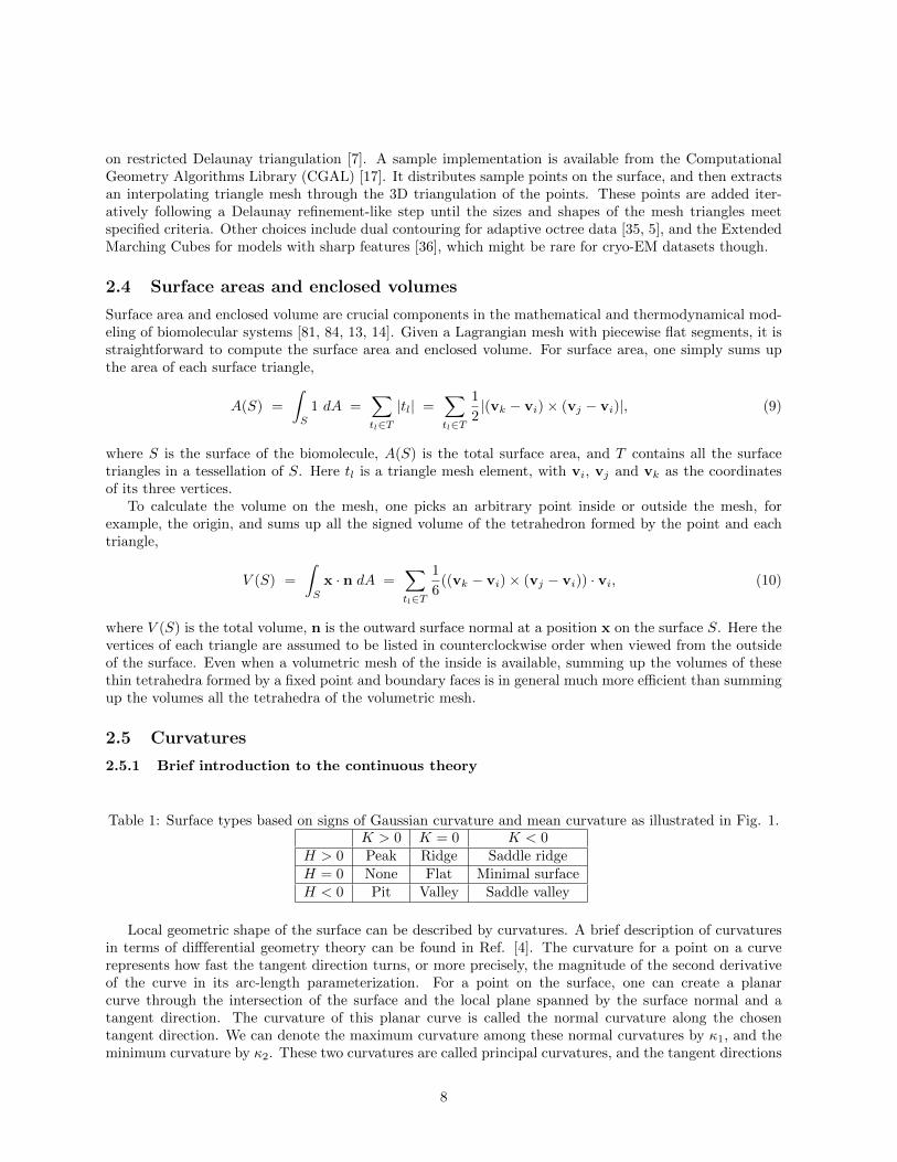
Table 1: Surface types based on signs of Gaussian curvature and mean curvature as illustrated in Fig. 1.K > 0 K = 0 K < 0

H > 0 Peak Ridge Saddle ridgeH = 0 None Flat Minimal surfaceH < 0 Pit Valley Saddle valley

Local geometric shape of the surface can be described by curvatures. A brief description of curvaturesin terms of diffferential geometry theory can be found in Ref. [4]. The curvature for a point on a curverepresents how fast the tangent direction turns, or more precisely, the magnitude of the second derivativeof the curve in its arc-length parameterization. For a point on the surface, one can create a planarcurve through the intersection of the surface and the local plane spanned by the surface normal and atangent direction. The curvature of this planar curve is called the normal curvature along the chosentangent direction. We can denote the maximum curvature among these normal curvatures by κ1, and theminimum curvature by κ2. These two curvatures are called principal curvatures, and the tangent directions

8

Figure 1: Representative image gallery of surface types based on signs of Gaussian curvature and meancurvature listed in Table 1.

associated with them are called principal directions. Note that these two directions are always orthogonalto each other. It can be further shown that the normal curvature κ along an arbitrary direction can bedetermined by κ1 and κ2 (the principal curvatures) and the angle θ that the chosen tangent direction makeswith the maximum curvature direction

κ = cos2(θ)κ1 + sin2(θ)κ2.

The second order approximation (quadric surface patch) around that point will be the same if twoprincipal curvatures are identical. To see this, we describe the neighborhood of a point on the surface bythe deviation of the surface from the tangent plane (a height function z = f(x, y) in a local coordinatesystem with the origin aligned to the point and the xy-plane aligned to the tangent plane). The secondorder approximation is

z =1

2

(x y

)Hess

(xy

)+ . . . ,

where Hess is the Hessian (the symmetric second derivative matrix) of f ,

Hess =

(∂2f∂x2

∂2f∂x∂y

∂2f∂x∂y

∂2f∂y2

).

The actual shape of the second order approximation depends only on the eigenvalues of Hess, becauseapplying a rotation in the tangent plane can diagonalize the Hessian. Thus we can align two local approxi-mation shapes through a rotation, as along as the diagonalized Hessians are the same. By the definition ofcurvature, one can immediately see that these eigenvalues are −κ1 and −κ2. Here, we follow the convention

9

Figure 2: Schematic illustration of curvature algorithms. Left: A typical “one-ring” neighborhood of avertex (v0); Middel: Flattening the one-ring by “cutting open” along the edge v0v1, we can measure the

angle deficit used in Gaussian curvature estimates, denoted here by 4θ = 2π −5∑i=1

θi. Right: Angles used

in the cotangent formula for the Laplace-Beltrami estimate of mean curvature.

in which bending towards the normal indicates a negative curvature, and bending away from the normalindicates a positive curvature. In this way, the curvatures for spheres will be positive. Note that someauthors use the opposite sign.

Alternatively, it is often advantageous to use the Gaussian curvature and the mean curvature definedby

K = κ1κ2, (11)

H =1

2(κ1 + κ2). (12)

where K is the Gaussian curvature, and H is the mean curvature. They correspond to, respectively, thedeterminant and half of the trace of the above Hessian matrix, which is another way of prescribing therotation invariants.

Based on the signs of the Gaussian curvature and the mean curvature, the neighborhood of a surfacepoint can be roughly classified as one of the eight different shapes, namely, pit, valley, saddle ridge, flat,minimal surface, saddle valley, ridge, and peak. In Table 1, we specify the type of shapes for each possiblecombination of signs. The actual shapes can be found in Fig. 1.

Considering the quadratic approximations they represent, we can see that local shapes with oppositesigns of mean curvatures and same signs of Gaussian curvatures may fit together.

To give intuitive descriptions of the shape, another pair of continuous variables, the shape index s andthe curvedness c can also be defined [37]

s = − 2

πarctan

(κ1 + κ2

κ1 − κ2

),

c =

√1

2(κ2

1 + κ22).

Here s describes the relation between the principal curvatures and c describes how non-flat the shape is.

2.5.2 Curvature estimates on triangle meshes

In this work, we employ triangle meshes for the geometric representation of macromolecules. Therefore,we discuss schemes for curvature calculation on the triangle meshes.

10

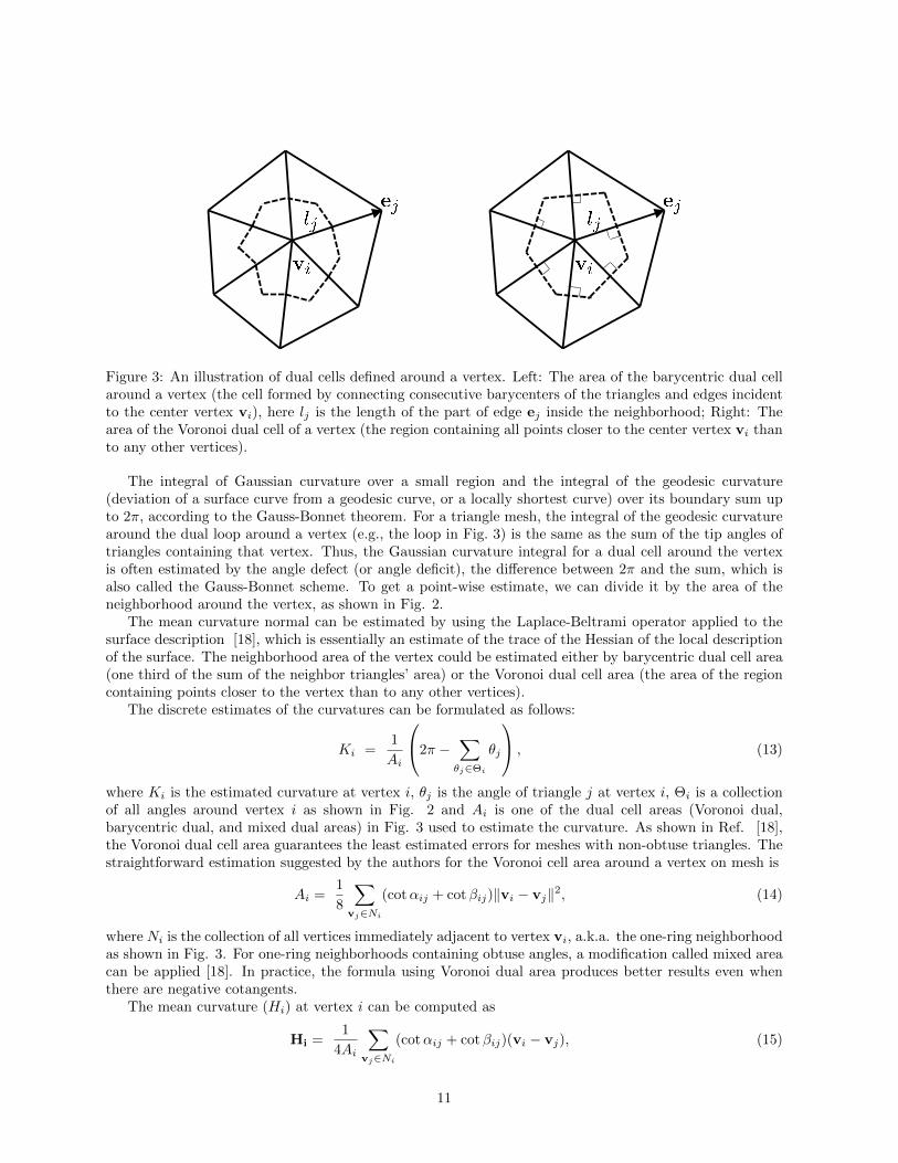
Figure 3: An illustration of dual cells defined around a vertex. Left: The area of the barycentric dual cellaround a vertex (the cell formed by connecting consecutive barycenters of the triangles and edges incidentto the center vertex vi), here lj is the length of the part of edge ej inside the neighborhood; Right: Thearea of the Voronoi dual cell of a vertex (the region containing all points closer to the center vertex vi thanto any other vertices).

The integral of Gaussian curvature over a small region and the integral of the geodesic curvature(deviation of a surface curve from a geodesic curve, or a locally shortest curve) over its boundary sum upto 2π, according to the Gauss-Bonnet theorem. For a triangle mesh, the integral of the geodesic curvaturearound the dual loop around a vertex (e.g., the loop in Fig. 3) is the same as the sum of the tip angles oftriangles containing that vertex. Thus, the Gaussian curvature integral for a dual cell around the vertexis often estimated by the angle defect (or angle deficit), the difference between 2π and the sum, which isalso called the Gauss-Bonnet scheme. To get a point-wise estimate, we can divide it by the area of theneighborhood around the vertex, as shown in Fig. 2.

The mean curvature normal can be estimated by using the Laplace-Beltrami operator applied to thesurface description [18], which is essentially an estimate of the trace of the Hessian of the local descriptionof the surface. The neighborhood area of the vertex could be estimated either by barycentric dual cell area(one third of the sum of the neighbor triangles’ area) or the Voronoi dual cell area (the area of the regioncontaining points closer to the vertex than to any other vertices).

The discrete estimates of the curvatures can be formulated as follows:

Ki =1

Ai

2π −∑θj∈Θi

θj

, (13)

where Ki is the estimated curvature at vertex i, θj is the angle of triangle j at vertex i, Θi is a collectionof all angles around vertex i as shown in Fig. 2 and Ai is one of the dual cell areas (Voronoi dual,barycentric dual, and mixed dual areas) in Fig. 3 used to estimate the curvature. As shown in Ref. [18],the Voronoi dual cell area guarantees the least estimated errors for meshes with non-obtuse triangles. Thestraightforward estimation suggested by the authors for the Voronoi cell area around a vertex on mesh is

Ai =1

8

∑vj∈Ni

(cotαij + cotβij)‖vi − vj‖2, (14)

where Ni is the collection of all vertices immediately adjacent to vertex vi, a.k.a. the one-ring neighborhoodas shown in Fig. 3. For one-ring neighborhoods containing obtuse angles, a modification called mixed areacan be applied [18]. In practice, the formula using Voronoi dual area produces better results even whenthere are negative cotangents.

The mean curvature (Hi) at vertex i can be computed as

Hi =1

4Ai

∑vj∈Ni

(cotαij + cotβij)(vi − vj), (15)

11

where Hi = Hini is the mean curvature normal, and ni is a unit vector representing an estimated surfacenormal at vertex i. The sign of Hi can be determined by the sign of Hi · n, where n is the normal of anyof the triangles incident to vertex i. Here vi and vj are the coordinates of vertex i and j, αij and βij arethe opposite angles of the same edge in two triangles incident to the edge (see, e.g., Fig. 2 Right).

If an estimated curvature tensor is required, a commonly used approach is to take the average of thecurvature tensor evaluated on the edges inside a certain neighborhood [16]

C(vi) =1

A′i

∑ej∈E(vi)

β(ej)lj ej eTj , (16)

where C(vi) is the estimated curvature tensor at vertex i expressed as a symmetric 3×3-matrix in the globalEuclidean coordinates, A′i is the area of a specific neighborhood (common choices include, for example, theintersection of a sphere with give radius around i, a geodesic disk on the surface around i, or the one-ringof vertex i). E(vi) is the set of all edges intersecting the neighborhood around vertex i, β(ej) is the signeddihedral angle between the normals of the faces sharing edge ej (negative when the faces bend towards thesurface normal and positive otherwise), ej the unit direction along ej (choosing either orientation of theedge will result in the same tensor), (·)T denotes the matrix transpose operation and lj is the length of thepart of edge ej inside the neighborhood. To find two principal curvatures and two principal directions, onemay perform an eigen-decomposition of C(vi). The eigenvalue with the smallest absolute value is alwaysnearly 0, and the associated eigenvector is an estimate of the local surface normal. Other two eigenvaluesare the principal curvatures, and their associated eigenvectors are two principal directions in the tangentplane. The larger the chose neighborhood is, the less accurate the result is. However, choosing an overlysmall neighborhood results in noisy estimates when the resolution of the mesh is low.

2.6 Volumetric meshing

Volumetric meshing refers to the interior meshing. It is possible to generate tetrahedron meshes directlyfrom 3D images with theoretical bounds on dihedral angles using algorithms such as isosurface stuffing[39]. Isosurface stuffing uses regular patterns to tetrahedralize grid cells completely inside the surface,followed by a marching-cubes-like boundary treatment, which shifts some of grid points near the boundaryfor attaining a better element shape. The algorithm is extremely fast, and the surface can approximatesmooth iso-surfaces well under reasonable assumptions, but the element shape is not optimal, and itsadaptivity is restricted to octree-like structures.

Other available popular algorithms include TetGen [63] and NetGen [60], both providing user controlon the size and shape of tetrahedra. The NetGen can take either a constructive solid geometry (shapes com-posed of primitive shapes combined through Boolean operations, i.e, union, intersection, and subtraction)or a boundary surface representation (BRep). However, NetGen can be less robust than other algorithms,such as TetGen [41]. TetGen produces tetrahedron meshes through constrained Delaunay tetrahedraliza-tion. If the tetrahedron mesh is required to conform to a boundary triangle mesh, the TetGen can bethe method of choice. However, restricting the boundary to the given mesh can make the quality of thevolumetric mesh dependent on the surface triangle mesh given by the user.

Another recent algorithm using interleaved Delaunay refinement and mesh optimization [71] can gen-erate quality meshes that satisfy a set of user-defined criteria, which can be useful, for example, whenimportance of the sampling density is determined by the local chemical structure. In the Delaunay re-finement step, sample points are inserted in order to satisfy the user-specified quality requirements. Inthe optimization step, a target function called the optimal Delaunay triangulation energy is used, whoseminimization leads to a high quality mesh. A final step perturbing the locations of vertices of slivers (flattetrahedra) further improves the mesh quality.

12

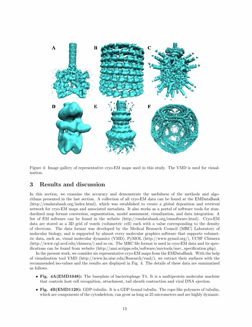
Figure 4: Image gallery of representative cryo-EM maps used in this study. The VMD is used for visual-ization.

3 Results and discussion

In this section, we examine the accuracy and demonstrate the usefulness of the methods and algo-rithms presented in the last section. A collection of all cryo-EM data can be found at the EMDataBank(http://emdatabank.org/index.html), which was established to create a global deposition and retrievalnetwork for cryo-EM maps and associated metadata. It also works as a portal of software tools for stan-dardized map format conversion, segmentation, model assessment, visualization, and data integration. Alist of EM software can be found in the website (http://emdatabank.org/emsoftware.html). Cryo-EMdata are stored as a 3D grid of voxels (volumetric cell) each with a value corresponding to the densityof electrons. The data format was developed by the Medical Research Council (MRC) Laboratory ofmolecular biology, and is supported by almost every molecular graphics software that supports volumet-ric data, such as, visual molecular dynamics (VMD), PyMOL (http://www.pymol.org/), UCSF Chimera(http://www.cgl.ucsf.edu/chimera/) and so on. The MRC file format is used in cryo-EM data and its spec-ifications can be found from website (http://ami.scripps.edu/software/mrctools/mrc−specification.php).

In the present work, we consider six representative cryo-EM maps from the EMDataBank. With the helpof visualization tool VMD (http://www.ks.uiuc.edu/Research/vmd/), we extract their surfaces with therecommended iso-values and the results are displayed in Fig. 4. The details of these data are summarizedas follows.

• Fig. 4A(EMD1048): The baseplate of bacteriophage T4. It is a multiprotein molecular machinethat controls host cell recognition, attachment, tail sheath contraction and viral DNA ejection.

• Fig. 4B(EMD1129): GDP-tubulin. It is a GDP-bound tubulin. The rope-like polymers of tubulin,which are components of the cytoskeleton, can grow as long as 25 micrometers and are highly dynamic.

13

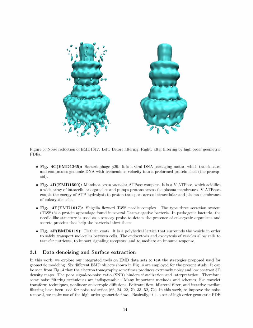
Figure 5: Noise reduction of EMD1617. Left: Before filtering; Right: after filtering by high order geometricPDEs.

• Fig. 4C(EMD1265): Bacteriophage φ29. It is a viral DNA-packaging motor, which translocatesand compresses genomic DNA with tremendous velocity into a preformed protein shell (the procap-sid).

• Fig. 4D(EMD1590): Manduca sexta vacuolar ATPase complex. It is a V-ATPase, which acidifiesa wide array of intracellular organelles and pumps protons across the plasma membranes. V-ATPasescouple the energy of ATP hydrolysis to proton transport across intracellular and plasma membranesof eukaryotic cells.

• Fig. 4E(EMD1617): Shigella flexneri T3SS needle complex. The type three secretion system(T3SS) is a protein appendage found in several Gram-negative bacteria. In pathogenic bacteria, theneedle-like structure is used as a sensory probe to detect the presence of eukaryotic organisms andsecrete proteins that help the bacteria infect them.

• Fig. 4F(EMD5119): Clathrin coats. It is a polyhedral lattice that surrounds the vesicle in orderto safely transport molecules between cells. The endocytosis and exocytosis of vesicles allow cells totransfer nutrients, to import signaling receptors, and to mediate an immune response.

3.1 Data denoising and Surface extraction

In this work, we explore our integrated tools on EMD data sets to test the strategies proposed used forgeometric modeling. Six different EMD objects shown in Fig. 4 are employed for the present study. It canbe seen from Fig. 4 that the electron tomography sometimes produces extremely noisy and low contrast 3Ddensity maps. The poor signal-to-noise ratio (SNR) hinders visualization and interpretation. Therefore,some noise filtering techniques are indispensable. Many important methods and schemes, like wavelettransform techniques, nonlinear anisotropic diffusions, Beltrami flow, bilateral filter, and iterative medianfiltering have been used for noise reduction [66, 24, 22, 70, 33, 52, 72]. In this work, to improve the noiseremoval, we make use of the high order geometric flows. Basically, it is a set of high order geometric PDE

14

Figure 6: Comparison of surface meshes. Top: Marching cubes result of EMD1590; Bottom: CGAL resultof EMD1590.

based low-pass filters for image processing or surface analysis. An example of noise removal of EMD1617is demonstrated in Fig. 5. The basic structure of the T3SS needle complex is preserved while the noiseamplitude is dramatically reduced. During the process of noise reduction, the surface of the protein issmoothed. The sharp edge and sharp tips are naturally removed. From the energy minimization pointof view, these features are not favorable in the protein surface formation [4]. Therefore, the loss of thesefeatures does not lead to degradation in accuracy when dealing with protein data.

Among those surface extraction methods we showed in Section 2.3, we compare the results of themarching cubes method and CGAL’s Delaunay-based method in Figure 6. The marching cubes methodis highly parallelizable because the lookup table used is precomputed and stored. For all the files thatwe tested, it costs less than five seconds to process a cryo-EM map with up to 200×200×200 Cartesiangrids. The direct result from marching cubes for EMD1590 shows that it may have a large number of skinnytriangles, and the overall shape may contain terracing artifacts for a large proportion of the triangles. Manytriangles have sharp angles less than 30◦. The lack of element quality control is the intrinsic weakness ofthe marching cubes methods. Thus, the result often needs post-processing to improve the mesh quality. Itmay also require a large number of triangles to store (14,170 vertices and 28,360 triangles in the exampleshown) at a given accuracy due to the lack of adaptivity.

On the other hand, CGAL’s running time and generated surface mesh quality depend heavily on thecriteria chosen for the Delaunay triangulation. The criteria are controlled by three parameters: angularbound for mesh triangles’ minimal angle, radius bound for the maximum surface Delaunay balls’ radius(a surface Delaunay ball circumscribes a mesh triangle and centered on surface), and distance bound forthe maximum distance between triangle’s circumcenter and surface Delaunay ball center. However, theseparameters can usually be easily tuned to achieve proper results with appropriate triangle shapes andsizes given some domain knowledge of the intended application. We use 30◦ as the angular bound, 0.8 asthe radius bound and 0.8 as the distance bound to directly extract the EMD1590 surface mesh from its

15

Figure 7: Comparison of surface mesh angle distributions. Left: Angle histogram of marching cubes resultof EMD1590; Right: Angle histogram of CGAL isosurface extraction result of EMD1590.

cryo-EM map file. It takes about four seconds to run the algorithm to get the extracted surface with 10,100vertices and 20,220 triangles. If we set smaller parameter values we will get more detailed models but maysuffer from longer running time and increased mesh size due to the smaller mesh triangles. Compared tothe marching cubes result for EMD1590, the CGAL result gives triangle angles always greater than 30degrees, triangles with almost the same size, and reduced mesh sizes without losing surface shape accuracy,as shown in Fig. 6.

The histograms of the triangle angle for both meshes are given in Fig. 7. From the figure one cansee that the angles in the marching cubes results have a large distribution in the low range, which mayresult in accuracy problems in mathematical modeling involving PDEs. In contrast, CGAL’s results areguaranteed to meet the angle requirements while reducing the mesh size significantly.

3.2 Surface mesh improvement

Figure 8: Mesh improvement with Delaunay remeshing. Left: marching cubes result of EMD1590; Right:remeshing result using the result to the left as the input.

The surface generated from the marching cubes method or its variants often does not fit the needof applications relying on finite element, finite difference, or finite volume methods, such as geometricreconstruction of the internal structure or numerical simulation of electrostatics [89, 90, 81, 13, 14]. Theprocess of creating a mesh that satisfies the new requirements while remaining close to the original mesh iscalled remeshing [1]. For instance, the mesh for EMD1590 produced by the marching cubes method can beremeshed into a mesh with rather uniform well-shaped triangles as shown in Fig. 8. Even for meshes withwell-shaped elements (for triangle meshes, this means nearly equilateral triangles, measured by the ratio of

16

the circumcircle radius to the length of the shortest edge [62]), it is still possible to perform remeshing toreduce vertex count while remaining faithful to the original underlying surface. In this case, the procedureis also called mesh simplification.

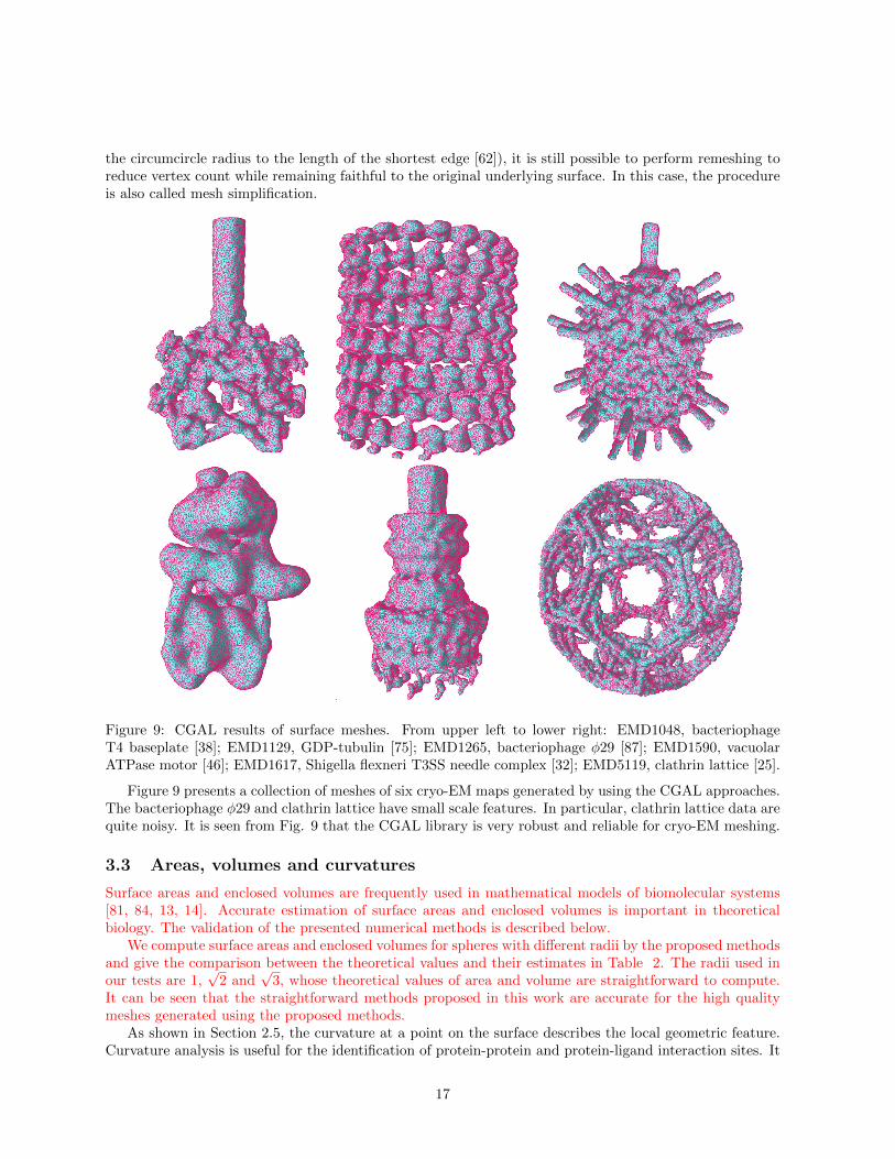
Figure 9: CGAL results of surface meshes. From upper left to lower right: EMD1048, bacteriophageT4 baseplate [38]; EMD1129, GDP-tubulin [75]; EMD1265, bacteriophage φ29 [87]; EMD1590, vacuolarATPase motor [46]; EMD1617, Shigella flexneri T3SS needle complex [32]; EMD5119, clathrin lattice [25].

Figure 9 presents a collection of meshes of six cryo-EM maps generated by using the CGAL approaches.The bacteriophage φ29 and clathrin lattice have small scale features. In particular, clathrin lattice data arequite noisy. It is seen from Fig. 9 that the CGAL library is very robust and reliable for cryo-EM meshing.

3.3 Areas, volumes and curvatures

Surface areas and enclosed volumes are frequently used in mathematical models of biomolecular systems[81, 84, 13, 14]. Accurate estimation of surface areas and enclosed volumes is important in theoreticalbiology. The validation of the presented numerical methods is described below.

We compute surface areas and enclosed volumes for spheres with different radii by the proposed methodsand give the comparison between the theoretical values and their estimates in Table 2. The radii used inour tests are 1,

√2 and

√3, whose theoretical values of area and volume are straightforward to compute.

It can be seen that the straightforward methods proposed in this work are accurate for the high qualitymeshes generated using the proposed methods.

As shown in Section 2.5, the curvature at a point on the surface describes the local geometric feature.Curvature analysis is useful for the identification of protein-protein and protein-ligand interaction sites. It

17

Table 2: Comparison of theoretical values and computer estimate of sphere’s areas and volumes.radius total area (est.) total area (theo.) total volume (est.) total volume (theo.)

1 12.53 12.57 4.16 4.19√2 25.09 25.13 11.81 11.85√3 37.66 37.70 21.72 21.77

Table 3: The curvatures estimated using barycentric dual cell area. Here µK (resp., µH) is the averageof Gaussian curvature K (mean curvature H), σ2

K (σ2H) is the standard deviation of K (H), and Ktheo

(Htheo) is the theoretical value of K (H).radius µK σ2

K Ktheo µH σ2H Htheo

1 1.003239 0.026352 1 1.000031 0.018632 1√2 0.500804 0.011344 0.5 0.707106 0.011323 0.707107√3 0.333685 0.009292 0.333333 0.577343 0.010881 0.577350

can also be used to help understand the protein-DNA binding specificity. In this work, we first validate theaccuracy and convergence order of the numerical methods proposed in Section 2.5. We then demonstratethe usefulness of these methods for cryo-EM data analysis.

Figure 10: The analytical geometry model: a patch of a sphere.

As discussed in Section 2.5, around each vertex, the one-ring area can be chosen in two differentways, the barycentric dual cell area and the Voronoi cell area. The accuracy of these approaches areexamined by spheres of radii (r) 1,

√2 and

√3. Their Gaussian and mean curvatures are given by 1/r2

and 1/r, respectively. These spheres are tessellated with triangles of similar sizes. The results of estimatedcurvatures obtained with the barycentric dual areas are shown in Table 3, together with theoretical values.Both our results for both Gaussian and mean curvatures are accurate in the tests. The resulting standarddeviations show that the difference between the computed value and the theoretical value is small relativeto the mesh size. For a comparison, we also listed our results obtained with the Voronoi dual areas inTable 4, under the same mesh. It is seen that the curvatures computed with the Voronoi dual areas areessentially the same as those with the barycentric dual areas. However, the Voronoi dual area approachoffers smaller standard deviations in Gaussian and mean curvature estimations than does the barycentricdual area approach. Therefore, the Voronoi dual area approach performs better and is utilized in the rest

18

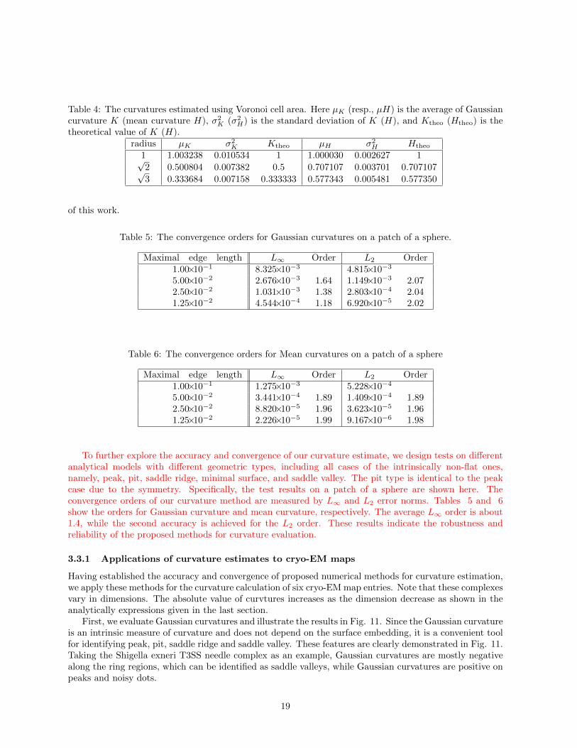
Table 4: The curvatures estimated using Voronoi cell area. Here µK (resp., µH) is the average of Gaussiancurvature K (mean curvature H), σ2

K (σ2H) is the standard deviation of K (H), and Ktheo (Htheo) is the

theoretical value of K (H).radius µK σ2

K Ktheo µH σ2H Htheo

1 1.003238 0.010534 1 1.000030 0.002627 1√2 0.500804 0.007382 0.5 0.707107 0.003701 0.707107√3 0.333684 0.007158 0.333333 0.577343 0.005481 0.577350

of this work.

Table 5: The convergence orders for Gaussian curvatures on a patch of a sphere.

Maximal edge length L∞ Order L2 Order1.00×10−1 8.325×10−3 4.815×10−3

5.00×10−2 2.676×10−3 1.64 1.149×10−3 2.072.50×10−2 1.031×10−3 1.38 2.803×10−4 2.041.25×10−2 4.544×10−4 1.18 6.920×10−5 2.02

Table 6: The convergence orders for Mean curvatures on a patch of a sphere

Maximal edge length L∞ Order L2 Order1.00×10−1 1.275×10−3 5.228×10−4

5.00×10−2 3.441×10−4 1.89 1.409×10−4 1.892.50×10−2 8.820×10−5 1.96 3.623×10−5 1.961.25×10−2 2.226×10−5 1.99 9.167×10−6 1.98

To further explore the accuracy and convergence of our curvature estimate, we design tests on differentanalytical models with different geometric types, including all cases of the intrinsically non-flat ones,namely, peak, pit, saddle ridge, minimal surface, and saddle valley. The pit type is identical to the peakcase due to the symmetry. Specifically, the test results on a patch of a sphere are shown here. Theconvergence orders of our curvature method are measured by L∞ and L2 error norms. Tables 5 and 6show the orders for Gaussian curvature and mean curvature, respectively. The average L∞ order is about1.4, while the second accuracy is achieved for the L2 order. These results indicate the robustness andreliability of the proposed methods for curvature evaluation.

3.3.1 Applications of curvature estimates to cryo-EM maps

Having established the accuracy and convergence of proposed numerical methods for curvature estimation,we apply these methods for the curvature calculation of six cryo-EM map entries. Note that these complexesvary in dimensions. The absolute value of curvtures increases as the dimension decrease as shown in theanalytically expressions given in the last section.

First, we evaluate Gaussian curvatures and illustrate the results in Fig. 11. Since the Gaussian curvatureis an intrinsic measure of curvature and does not depend on the surface embedding, it is a convenient toolfor identifying peak, pit, saddle ridge and saddle valley. These features are clearly demonstrated in Fig. 11.Taking the Shigella exneri T3SS needle complex as an example, Gaussian curvatures are mostly negativealong the ring regions, which can be identified as saddle valleys, while Gaussian curvatures are positive onpeaks and noisy dots.

19

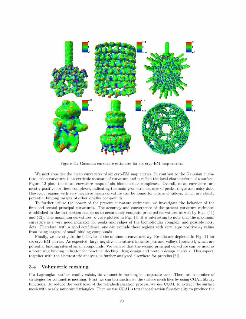
Figure 11: Gaussian curvature estimates for six cryo-EM map entries.

We next consider the mean curvatures of six cryo-EM map entries. In contrast to the Gaussian curva-ture, mean curvature is an extrinsic measure of curvature and it reflect the local characteristic of a surface.Figure 12 plots the mean curvature maps of six biomolecular complexes. Overall, mean curvatures aremostly positive for these complexes, indicating the main geometric features of peaks, ridges and noisy dots.However, regions with very negative mean curvature can be found for pits and valleys, which are clearlypotential binding targets of other smaller compounds.

To further utilize the power of the present curvature estimates, we investigate the behavior of thefirst and second principal curvatures. The accuracy and convergence of the present curvature estimatesestablished in the last section enable us to accuractely compute principal curvatures as well by Eqs. (11)and (12). The maximum curvatures, κ1, are plotted in Fig. 13. It is interesting to note that the maximumcurvature is a very good indicator for peaks and ridges of the biomolecular complex, and possible noisydots. Therefore, with a good confidence, one can exclude these regions with very large positive κ1 valuesfrom being targets of small binding compounds.

Finally, we investigate the behavior of the minimum curvature, κ2. Results are depicted in Fig. 14 forsix cryo-EM entries. As expected, large negative curvatures indicate pits and valleys (pockets), which arepotential binding sites of small compounds. We believe that the second principal curvature can be used asa promising binding indicator for practical docking, drug design and protein design analysis. This aspect,together with the electrostatic analysis, is further analyzed elsewhere for proteins [21].

3.4 Volumetric meshing

If a Lagrangian surface readily exists, its volumetric meshing is a separate task. There are a number ofstrategies for volumetric meshing. First, we can tetrahedralize the surface mesh files by using CGAL libraryfunctions. To reduce the work load of the tetrahedralization process, we use CGAL to extract the surfacemesh with nearly same sized triangles. Then we use CGAL’s tetrahedralization functionality to produce the

20

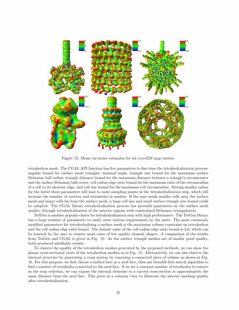
Figure 12: Mean curvature estimates for six cryo-EM map entries.

tetrahedron mesh. The CGAL API function has five parameters to fine-tune the tetrahedralization process:angular bound for surface mesh triangles’ minimal angle, triangle size bound for the maximum surfaceDelaunay ball radius, triangle distance bound for the maximum distance between a triangle’s circumcenterand the surface Delaunay ball center, cell radius edge ratio bound for the maximum ratio of the circumradiusof a cell to its shortest edge, and cell size bound for the maximum cell circumradius. Setting smaller valuesfor the latter three parameters will lead to more sampling points in the tetrahedralization step, which willincrease the number of vertices and tetrahedra in meshes. If the user needs smaller cells near the surfacemesh and larger cells far from the surface mesh, a large cell size and small surface triangle size bound couldbe adopted. The CGAL library tetrahedralization process has provable guarantees on the surface meshquality, through tetrahedralization of the interior regions with constrained Delaunay triangulation.

TetGen is another popular choice for tetrahedralization step with high performance. The TetGen libraryhas a large number of parameters to easily meet various requirements by the users. The most commonlymodified parameters for tetrahedralizing a surface mesh is the maximum volume constraint on tetrahedronand the cell radius edge ratio bound. The default value of the cell radius edge ratio bound is 2.0, which canbe lowered by the user to remove most cases of low quality element shapes. A comparison of the resultsfrom TetGen and CGAL is given in Fig. 15. As the surface triangle meshes are of similar good quality,both produced satisfiable results.

To observe the quality of the tetrahedron meshes generated by the proposed methods, we can show theplanar cross-sectional views of the tetrahedron meshes as in Fig. 15. Alternatively, we can also observe theinternal structure by generating a cross section by removing a connected piece of volume as shown in Fig.16. For this purpose, we first choose a surface face as a seed face, then use breadth-first search algorithm tofind a number of tetrahedra connected to the seed face. If we set a constant number of tetrahedra to removeas the stop criterion, we can expose the internal elements in a curved cross-section at approximately thesame distance from the seed face. This gives us a cutaway view to illustrate the interior meshing qualityafter tetrahedralization.

21

Figure 13: Maximum curvature (κ1) estimates for six cryo-EM map entries.

Both CGAL and TetGen share a parameter to tune the cell radius edge ratio bound of a generatedtetrahedron. This parameter is highly effective in controlling the quality of the tetrahedra. All well shapedtetrahedra have small values (less than 3) for the ratio, and most of the badly shaped tetrahedra havelarge values. This does not mean that the limit can be set arbitrarily small, because the value has a lowerbound of 0.612 (the value for an equilateral tetrahedron). The one case of a badly shaped tetrahedron withsmall (cell radius to shortest edge) ratio is called “sliver”, which has a flat and near-degenerate shape. Itscell radius edge ratio can go as low as 0.707. One effective way to prevent slivers from being created is toincorporate a minimum volume constraint, or to employ a procedure called sliver exudation as is done inCGAL.

4 Conclusion

One of the most important new trends in structural biology is the investigation of the structures, functionsand dynamics of subcellular structures, organelles and large multiprotein complexes. Currently, a mainworkhorse for this investigation is the cryo-electron microscopy (cryo-EM). However, cryo-EM maps arewell known for their low resolution and low reliability. Geometric modeling provides tools for improvingcryo-EM resolution, and bridges the gap between molecular structures and mathematical modeling, which isnecessary for the understanding of the function and dynamics of subcellular structures and complexes. Thiswork presents a comprehensive protocol for the geometric modeling of cryo-EM data and other volumetricdensity distributions used in macromolecules. We first introduce high order geometric partial differentialequations (PDEs) for noise removal of cryo-EM data and volumetric data. High order geometric PDEs aremore efficient for denoising because they have controllable time-frequency localization and can be tuned upfor specific noise distribution. Additionally, we discuss two surface extraction schemes, the regular marchingcubes and the Computational Geometry Algorithms Library (CGAL). Moreover, we explore efficient and

22

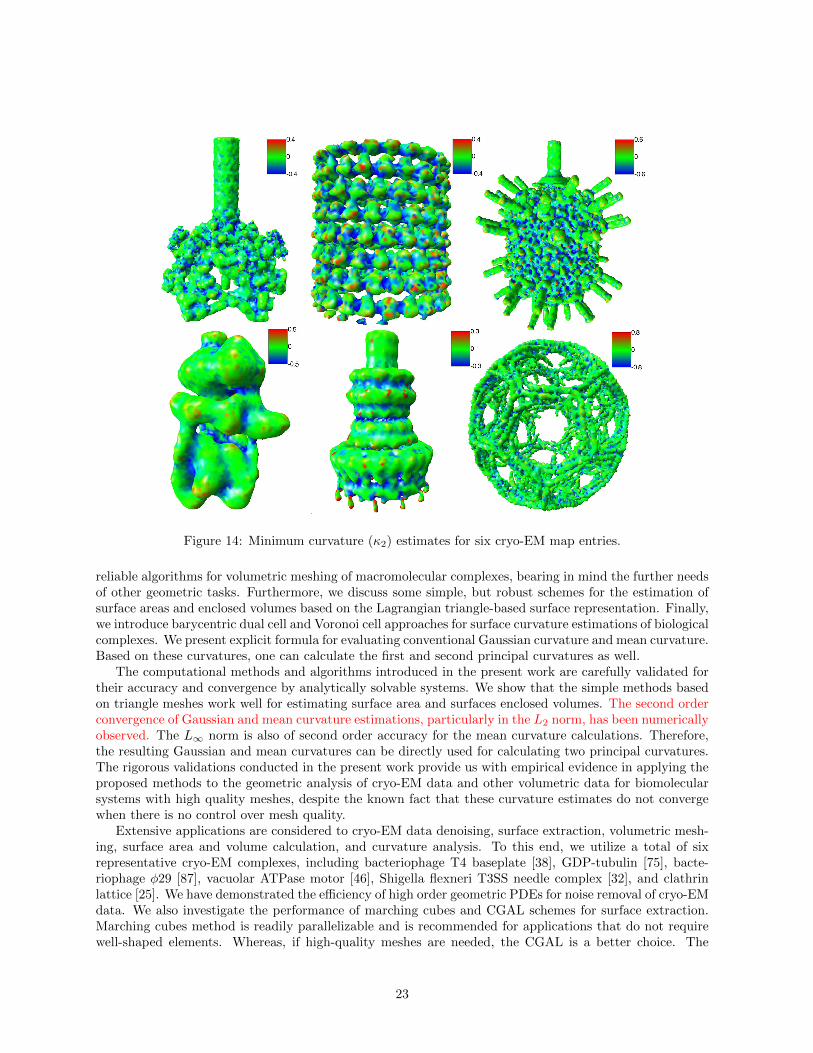
Figure 14: Minimum curvature (κ2) estimates for six cryo-EM map entries.

reliable algorithms for volumetric meshing of macromolecular complexes, bearing in mind the further needsof other geometric tasks. Furthermore, we discuss some simple, but robust schemes for the estimation ofsurface areas and enclosed volumes based on the Lagrangian triangle-based surface representation. Finally,we introduce barycentric dual cell and Voronoi cell approaches for surface curvature estimations of biologicalcomplexes. We present explicit formula for evaluating conventional Gaussian curvature and mean curvature.Based on these curvatures, one can calculate the first and second principal curvatures as well.

The computational methods and algorithms introduced in the present work are carefully validated fortheir accuracy and convergence by analytically solvable systems. We show that the simple methods basedon triangle meshes work well for estimating surface area and surfaces enclosed volumes. The second orderconvergence of Gaussian and mean curvature estimations, particularly in the L2 norm, has been numericallyobserved. The L∞ norm is also of second order accuracy for the mean curvature calculations. Therefore,the resulting Gaussian and mean curvatures can be directly used for calculating two principal curvatures.The rigorous validations conducted in the present work provide us with empirical evidence in applying theproposed methods to the geometric analysis of cryo-EM data and other volumetric data for biomolecularsystems with high quality meshes, despite the known fact that these curvature estimates do not convergewhen there is no control over mesh quality.

Extensive applications are considered to cryo-EM data denoising, surface extraction, volumetric mesh-ing, surface area and volume calculation, and curvature analysis. To this end, we utilize a total of sixrepresentative cryo-EM complexes, including bacteriophage T4 baseplate [38], GDP-tubulin [75], bacte-riophage φ29 [87], vacuolar ATPase motor [46], Shigella flexneri T3SS needle complex [32], and clathrinlattice [25]. We have demonstrated the efficiency of high order geometric PDEs for noise removal of cryo-EMdata. We also investigate the performance of marching cubes and CGAL schemes for surface extraction.Marching cubes method is readily parallelizable and is recommended for applications that do not requirewell-shaped elements. Whereas, if high-quality meshes are needed, the CGAL is a better choice. The

23

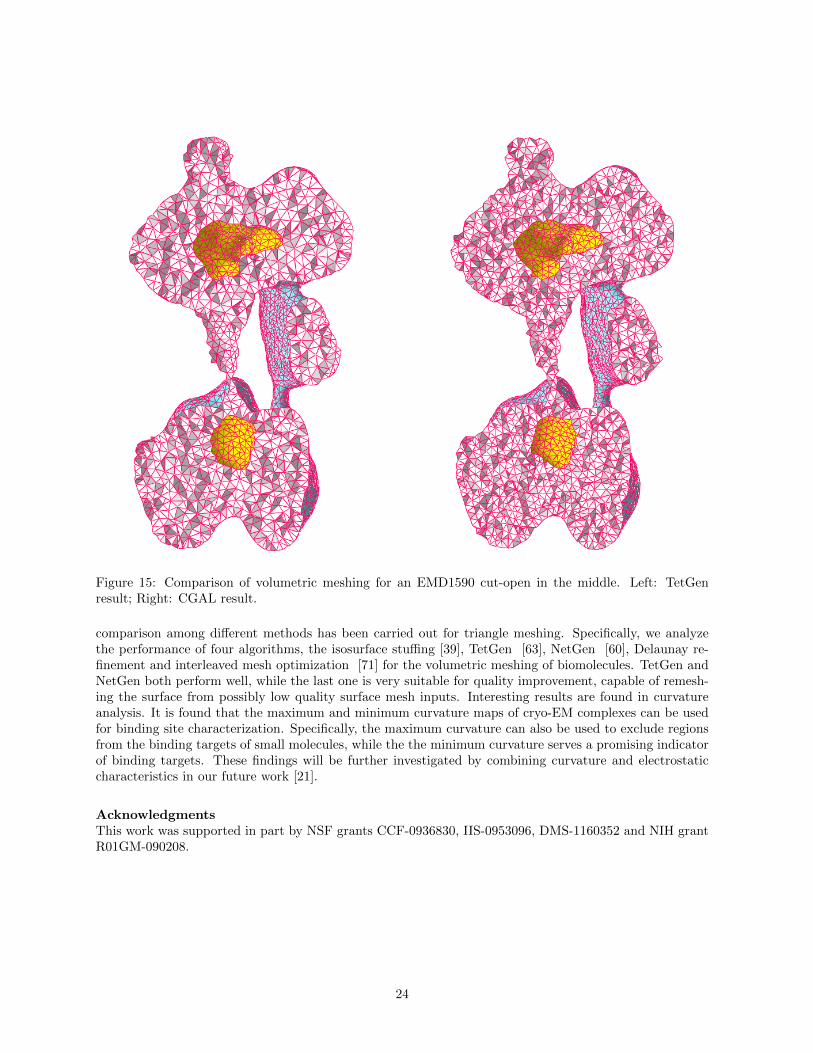
Figure 15: Comparison of volumetric meshing for an EMD1590 cut-open in the middle. Left: TetGenresult; Right: CGAL result.

comparison among different methods has been carried out for triangle meshing. Specifically, we analyzethe performance of four algorithms, the isosurface stuffing [39], TetGen [63], NetGen [60], Delaunay re-finement and interleaved mesh optimization [71] for the volumetric meshing of biomolecules. TetGen andNetGen both perform well, while the last one is very suitable for quality improvement, capable of remesh-ing the surface from possibly low quality surface mesh inputs. Interesting results are found in curvatureanalysis. It is found that the maximum and minimum curvature maps of cryo-EM complexes can be usedfor binding site characterization. Specifically, the maximum curvature can also be used to exclude regionsfrom the binding targets of small molecules, while the the minimum curvature serves a promising indicatorof binding targets. These findings will be further investigated by combining curvature and electrostaticcharacteristics in our future work [21].

AcknowledgmentsThis work was supported in part by NSF grants CCF-0936830, IIS-0953096, DMS-1160352 and NIH grantR01GM-090208.

24

Figure 16: Cross-section view of CGAL result of EMD1590.

References[1] P. Alliez, G. Ucelli, C. Gotsman, and M. Attene. Recent advances in remeshing of surfaces. In Leila de Floriani and

Michela Spagnuolo, editor, Shape Analysis and Structuring, pages 53–82. Springer-Verlag, 2007.

[2] P. W. Bates, Z. Chen, Y. H. Sun, G. W. Wei, and S. Zhao. Geometric and potential driving formation and evolution ofbiomolecular surfaces. J. Math. Biol., 59:193–231, 2009.

[3] P. W. Bates, G. W. Wei, and S. Zhao. The minimal molecular surface. arXiv:q-bio/0610038v1, [q-bio.BM], 2006.

[4] P. W. Bates, G. W. Wei, and S. Zhao. Minimal molecular surfaces and their applications. Journal of ComputationalChemistry, 29(3):380–91, 2008.

[5] S. Bischoff, D. Pavic, and L. Kobbelt. Automatic restoration of polygon models. ACM Trans. Graph., 24(4):1332–1352,Oct. 2005.

[6] P. Blomgren and T. Chan. Color TV: total variation methods for restoration of vector-valued images. Image Processing,IEEE Transactions on, 7(3):304–309, 1998.

[7] J.-D. Boissonnat and S. Oudot. Provably good sampling and meshing of surfaces. Graph. Models, 67(5):405–451, Sept.2005.

[8] M. Botsch, L. Kobbelt, M. Pauly, P. Alliez, and B. Levy. Polygon Mesh Processing. Ak Peters Series. A K Peters, 2010.

[9] V. Carstensen, R. Kimmel, and G. Sapiro. Geodesic active contours. International Journal of Computer Vision, 22:61–79,1997.

[10] A. Chambolle and P. L. Lions. Image recovery via total variation minimization and related problems. NumerischeMathematik, 76(2):167–188, 1997.

[11] T. Chan, A. Marquina, and P. Mulet. High-order total variation-based image restoration. SIAM Journal on ScientificComputing, 22(2):503–516, 2000.

[12] D. Chen, Z. Chen, and G. W. Wei. Quantum dynamics in continuum for proton transport II: Variational solvent-soluteinterface. International Journal for Numerical Methods in Biomedical Engineering, 28:25 – 51, 2012.

[13] Z. Chen, N. A. Baker, and G. W. Wei. Differential geometry based solvation models I: Eulerian formulation. J. Comput.Phys., 229:8231–8258, 2010.

[14] Z. Chen, N. A. Baker, and G. W. Wei. Differential geometry based solvation models II: Lagrangian formulation. J.Math. Biol., 63:1139– 1200, 2011.

[15] G. Cipriano, G. N. Phillips Jr., and M. Gleicher. Multi-scale surface descriptors. IEEE Transactions on Visualizationand Computer Graphics, 15:1201–1208, 2009.

[16] D. Cohen-Steiner and J.-M. Morvan. Second fundamental measure of geometric sets and local approximation of curvatures. J. Diff. Geom., 74(3):391–404, 2006.

[17] G. Damiand. Combinatorial maps. In CGAL User and Reference Manual. CGAL Editorial Board, 4.0 edition, 2012.www.cgal.org/Manual/4.0/doc html/cgal manual/packages.html#Pkg:CombinatorialMaps.

25

[18] M. Desbrun, M. Meyer, P. Schroder, and A. Barr. Implicit fairing of irregular meshes using diffusion and curvature flow.ACM SIGGRAPH, pages 317–324, 1999.

[19] V. d’Otreppe, R. Boman, and J.-P. Ponthot. Generating smooth surface meshes from multi-region medical images.International Journal for Numerical Methods in Biomedical Engineering, 28:642–660, 2012.

[20] Q. Du, V. Faber, and M. Gunzburger. Centroidal voronoi tessellations: Applications and algorithms. SIAM Review,41(4):637–676, 1999.

[21] X. Feng, K. Xia, Y. Tong, and G.-W. Wei. Geometric and topological modeling of macromolecules I: Surface generation,meshing and classification. Journal of Molecular Graphics and Modelling, submitted 2012.

[22] J. J. Fernandez. Tomobflow: feature-preserving noise filtering for electron tomography. BMC Bioinformatics, 178:1–10,2009.

[23] J. J. Fernandez and S. Li. An improved algorithm for anisotropic nonlinear diffusion for denoising cryo-tomograms. J.Struct. Biol., 144:152C161, 2003.

[24] J. J. Fernandez, S. Li, and V. Lucic. Three-dimensional anisotropic noise reduction with automated parameter tuning:Application to electron cryotomography. In Current Topics in Artificial Intelligence, volume 4788, pages 60–69, 2007.

[25] A. Fotin, Y. Cheng, P. Sliz, N. Grigorieff, and S. C. Harrison et al. Molecular model for a complete clathrin lattice fromelectron cryomicroscopy. Nature, 432(7017):573–9–, Dec. 2004.

[26] A. S. Frangakis and R. Hegerl. Noise reduction in electron tomographic reconstructions using nonlinear anisotropicdiffusion. J. Struct. Biol., 135:239C250, 2001.

[27] P. L. George, F. Hecht, and E. Saltel. Automatic mesh generator with specified boundary. Computer Methods in AppliedMechanics and Engineering, 92:269– 288, 1991.

[28] G. Gilboa, N. Sochen, and Y. Y. Zeevi. Forward-and-backward diffusion processes for adaptive image enhancement anddenoising. IEEE Transactions on Image Processing, 11(7):689–703, 2002.

[29] G. Gilboa, N. Sochen, and Y. Y. Zeevi. Image sharpening by flows based on triple well potentials. Journal of MathematicalImaging and Vision, 20(1-2):121–131, 2004.

[30] J. B. Greer and A. L. Bertozzi. H-1 solutions of a class of fourth order nonlinear equations for image processing. Discreteand Continuous Dynamical Systems, 10(1-2):349–366, 2004.

[31] J. B. Greer and A. L. Bertozzi. Traveling wave solutions of fourth order PDEs for image processing. SIAM Journal onMathematical Analysis, 36(1):38–68, 2004.

[32] J. L. Hodgkinson, A. Horsley, D. Stabat, M. Simon, and S. Johnson et al. Three-dimensional reconstruction of theshigella t3ss transmembrane regions reveals 12-fold symmetry and novel features throughout. Nat Struct Mol Biol,16(5):477–85–, May 2009.

[33] W. Jiang, M. L. Baker, Q. Wu, C. Bajaj, and W. Chiu. Applications of a bilateral denoising filter in biological electronmicroscopy. J. Struct. Biol., 144:114C122, 2003.

[34] L. L. Ju, Q. Du, and M. Gunzburger. Probabilistic methods for centroidal voronoi tessellations and their parallelimplementations. Parallel Computing, 28:1477C1500, 2002.

[35] T. Ju, F. Losasso, S. Schaefer, and J. Warren. Dual contouring of hermite data. ACM Trans. Graph. (SIGGRAPH),21(3):339–346, July 2002.

[36] L. P. Kobbelt, M. Botsch, U. Schwanecke, and H.-P. Seidel. Feature sensitive surface extraction from volume data. InProceedings of the 28th annual conference on Computer graphics and interactive techniques, SIGGRAPH ’01, pages57–66, New York, NY, USA, 2001. ACM.

[37] J. J. Koenderink and A. J. van Doorn. Surface shape and curvature scales. Image and Vision Computing, 10(8):557–564,Oct. 1992.

[38] V. A. Kostyuchenko, P. G. Leiman, P. R. Chipman, S. Kanamaru, and M. J. van Raaij et al. Three-dimensional structureof bacteriophage t4 baseplate. Nat Struct Biol, 10(9):688–93–, Sept. 2003.

[39] F. Labelle and J. R. Shewchuk. Isosurface stuffing: fast tetrahedral meshes with good dihedral angles. ACM Trans.Graph. (SIGGRAPH), 26(3), July 2007.

[40] A. Leis, B. Rockel, L. Andrees, and W. Baumeister. Visualizing cells at the nanoscale. Trends Biochem. Sci., 34:60C70,2009.

[41] M. Lizier, J. Shepherd, L. Nonato, J. Comba, and C. Silva. Comparing techniques for tetrahedral mesh generation. InInaugural International Conference of the Engineering Mechanics Institute, 2008.

[42] W. E. Lorensen and H. E. Cline. Marching cubes: a high resolution 3d surface reconstruction algorithm. ComputerGraphics, 21:163–169, 1987.

[43] M. Lysaker, A. Lundervold, and X. C. Tai. Noise removal using fourth-order partial differential equation with applicationto medical magnetic resonance images in space and time. IEEE Transactions on Image Processing, 12(12):1579–1590,2003.

26

[44] E. Marchandise, G. Compere, M. Willemet, G. Bricteux, C. Geuzaine, and J. F. Remacle. Quality meshing based onstl triangulations for biomedical simulations. International Journal for Numerical Methods in Biomedical Engineering,26:876–889, 2010.

[45] C. Montani, R. Scateni, and R. Scopigno. A modified look-up table for implicit disambiguation of Marching Cubes. TheVisual Computer, 10(6):353–355, June 1994.

[46] S. P. Muench, M. Huss, C. F. Song, C. Phillips, and H. Wieczorek et al. Cryo-electron microscopy of the vacuolar atpasemotor reveals its mechanical and regulatory complexity. J Mol Biol, 386(4):989–99–, Mar. 2009.

[47] D. Mumford and J. Shah. Optimal approximations by piecewise smooth functions and associated variational problems.Communications on Pure and Applied Mathematics, 42(5):577–685, 1989.

[48] S. Nickell, C. Kofler, A. P. Leis, and W. Baumeister. A visual approach to proteomics. Nat. Rev. Mol. Cell Biol.,7:225–230, 2006.

[49] S. Osher and R. P. Fedkiw. Level set methods: An overview and some recent results. J. Comput. Phys., 169(2):463–502,2001.

[50] S. Osher and L. I. Rudin. Feature-oriented image enhancement using shock filters. SIAM Journal on Numerical Analysis,27(4):919–940, 1990.

[51] S. Osher and J. Sethian. Fronts propagating with curvature-dependent speed: algorithms based on Hamilton-Jacobiformulations. Journal of computational physics, 79(1):12–49, 1988.

[52] R. S. Pantelic, C. Y. Rothnagel, R.and Huang, D. Muller, and D. Woolford et al. The discriminative bilateral filter: Anenhanced denoising filter for electron microscopy data. J. Struct. Biol., 155:395C408, 2006.

[53] P. Perona and J. Malik. Scale-space and edge-detection using anisotropic diffusion. IEEE Transactions on PatternAnalysis and Machine Intelligence, 12(7):629–639, 1990.

[54] C. V. Robinson, A. Sali, and W. Baumeister. The molecular sociology of the cell. Nature, 450:973C982, 2007.

[55] L. I. Rudin, S. Osher, and E. Fatemi. Nonlinear total variation based noise removal algorithms. In Proceedings ofthe eleventh annual international conference of the Center for Nonlinear Studies on Experimental mathematics : com-putational issues in nonlinear science, pages 259–268, Amsterdam, The Netherlands, The Netherlands, 1992. ElsevierNorth-Holland, Inc.

[56] P. H. Saksono, P. Nithiarasu, and I. Sazonov. Numerical prediction of heat transfer patterns in a subject-specific humanupper airway. Journal of Heat Transfer, 134(031022):1–9, 2012.

[57] G. Sapiro and D. L. Ringach. Anisotropic diffusion of multivalued images with applications to color filtering. ImageProcessing, IEEE Transactions on, 5(11):1582–1586, 1996.

[58] I. Sazonov and P. Nithiarasu. Semi-automatic surface and volume mesh generation for subject-specific biomedicalgeometries. International Journal for Numerical Methods in Biomedical Engineering, 28:133–157, 2012.

[59] I. Sazonov, S. Y. Yeo, L. T. Bevan, X. H. Xie, R. V. Loon, and P. Nithiarasu. Modelling pipeline for subject-specificarterial blood flowa review. International Journal for Numerical Methods in Biomedical Engineering, 27:1868–1910,2011.

[60] J. Schoberl. Netgen - an advancing front 2d/3d mesh generator based on abstract rules. Comput and Vis in Science,1(1):41–52, 1997.

[61] J. A. Sethian. Evolution, implementation, and application of level set and fast marching methods for advancing fronts.J. Comput. Phys., 169(2):503–555, 2001.

[62] J. R. Shewchuk. Delaunay Refinement Mesh Generation. PhD thesis, School of Computer Science, Carnegie MellonUniversity, Pittsburgh, Pennsylvania, May 1997. Available as Technical Report CMU-CS-97-137.

[63] H. Si. Constrained delaunay tetrahedral mesh generation and refinement. Finite Elem. Anal. Des., 46:33–46, January2010.

[64] N. Sochen, R. Kimmel, and R. Malladi. A general framework for low level vision. Image Processing, IEEE Transactionson, 7(3):310–318, 1998.

[65] H. Soltanianzadeh, J. P. Windham, and A. E. Yagle. A multidimensional nonlinear edge-preserving filter for magnetic-resonace image-restoration. IEEE Transactions on Image Processing, 4(2):147–161, 1995.

[66] A. Stoschek and R. Hegerl. Denoising of electron tomographic reconstructions using multiscale transformations. J.Struct. Biol., 120:257C265, 1997.

[67] Y. H. Sun, P. R. Wu, G. W. Wei, and G. Wang. Evolution-operator-based single-step method for image processing. Int.J. Biomed. Imaging, 83847:1–27, 2006.

[68] T. Tasdizen, R. Whitaker, P. Burchard, and S. Osher. Geometric surface processing via normal maps. Acm Transactionson Graphics, 22(4):1012–1033, 2003.

[69] E. I. Tocheva, Z. Li, and G. J. Jensen. Electron cryotomography. In Cold Spring Harb. Perspect. Biol., volume 2, pageA003442, 2010.

27

[70] C. Tomasi and R. Manduchi. Bilateral filtering for gray and color images. Proc. ICCV, 98:839C846, 1998.

[71] J. Tournois, C. Wormser, P. Alliez, and M. Desbrun. Interleaving delaunay refinement and optimization for practicalisotropic tetrahedron mesh generation. ACM Trans. Graph. (SIGGRAPH), 28(3):75:1–75:9, July 2009.

[72] P. van der Heide, X. P. Xu, B. J. Marsh, D. Hanein, and N. Volkmann. Efficient automatic noise reduction of electrontomographic reconstructions based on iterative median filtering. J. Struct. Biol., 158:196C204, 2007.

[73] N. Volkmann. Methods for segmentation and interpretation of electron tomographic reconstructions. In Methods Enzymol,volume 483, pages 31–46, 2010.

[74] M. Wan, Y. Wang, and D. S. Wang. Variational surface reconstruction based on delaunay triangulation and graph cut.Int. J. Numer. Meth. Engng, 85:206C229, 2011.

[75] H. Wang and E. Nogales. Nucleotide-dependent bending flexibility of tubulin regulates microtubule assembly. Nature,435(7044):911–5–, June 2005.

[76] Y. Wang, G. W. Wei, and S.-Y. Yang. Partial differential equation transform – Variational formulation and Fourieranalysis. International Journal for Numerical Methods in Biomedical Engineering, 27:1996–2020, 2011.

[77] Y. Wang, G. W. Wei, and S.-Y. Yang. Mode decomposition evolution equations. Journal of Scientific Computing,50:495–518, 2012.

[78] Y. Wang, G. W. Wei, and S.-Y. Yang. Selective extraction of entangled textures via adaptive pde transform. InternationalJournal in Biomedical Imaging, 2012:Article ID 958142, 2012.

[79] N. P. Weatherill and O. Hassan. Efficient three-dimensional delaunay triangulation with automatic point creation andimposed boundary constraints. Int. J. Numer. Meth. Engng, 37:2005–2039, 1994.

[80] G. W. Wei. Generalized Perona-Malik equation for image restoration. IEEE Signal Processing Letters, 6(7):165–167,1999.

[81] G. W. Wei. Differential geometry based multiscale models. Bulletin of Mathematical Biology, 72:1562 – 1622, 2010.

[82] G. W. Wei and Y. Q. Jia. Synchronization-based image edge detection. Europhysics Letters, 59(6):814–819, 2002.

[83] G. W. Wei, Y. H. Sun, Y. C. Zhou, and M. Feig. Molecular multiresolution surfaces. arXiv:math-ph/0511001v1, pages1 – 11, 2005.

[84] G.-W. Wei, Q. Zheng, Z. Chen, and K. Xia. Variational multiscale models for charge transport. SIAM Review, 54(4):56,2012.

[85] T. P. Witelski and M. Bowen. ADI schemes for higher-order nonlinear diffusion equations. Applied Numerical Mathe-matics, 45(2-3):331–351, 2003.

[86] A. Witkin. Scale-space filtering: A new approach to multi-scale description. Proceedings of IEEE International Confer-ence on Acoustic Speech Signal Processing, 9:150–153, 1984.

[87] Y. Xiang, M. Morais, A. Battisti, S. Grimes, P. Jardine, D. Anderson, and M. Rossmann. Structural changes ofbacteriophage phi29 upon dna packaging and release. EMBO J, 25(21):5229–39–, Nov. 2006.

[88] Y. You and M. Kaveh. Fourth-order partial differential equations for noise removal. IEEE Transactions on ImageProcessing, 9(10):1723–1730, 2002.

[89] S. N. Yu, W. H. Geng, and G. W. Wei. Treatment of geometric singularities in implicit solvent models. Journal ofChemical Physics, 126:244108, 2007.

[90] S. N. Yu and G. W. Wei. Three-dimensional matched interface and boundary (MIB) method for treating geometricsingularities. J. Comput. Phys., 227:602–632, 2007.

[91] Z. Yu, M. Holst, Y. Cheng, and J. A. McCammon. Feature-preserving adaptive mesh generation for molecular shapemodeling and simulation. Journal of Molecular Graphics and Modeling, 26:1370–1380, 2008.

[92] Z. Yu, M. Holst, T. Hayashi, C. L. Bajaj, and M. H. Ellisman et al. Three-dimensional geometric modeling of membrane-bound organelles in ventricular myocytes: Bridging the gap between microscopic imaging and mathematical simulation.Journal of Structural Biology, 164:304–313, 2008.

[93] Y. Zhang, C. Bajaj, and G. Xu. Surface smoothing and quality improvement of quadrilateral/hexahedral meshes withgeometric flow. Communications in Numerical Methods in Engineering, 25:1–18, 2009.

[94] S. Zhao. Pseudo-time-coupled nonlinear models for biomolecular surface representation and solvation analysis. Interna-tional Journal for Numerical Methods in Biomedical Engineering, 27:1964– 1981, 2012.

[95] Q. Zheng, S. Y. Yang, and G. W. Wei. Molecular surface generation using PDE transform. International Journal forNumerical Methods in Biomedical Engineering, 28:291–316, 2012.

28