mixed hodge structures associated to geometric variations donu
TRANSCRIPT

Cycles, Motives and Shimura VarietiesEditor: V. SrinivasCopyright c!2010 Tata Institute of Fundamental ResearchPublisher: Narosa Publishing House, New Delhi, India
Mixed Hodge Structures Associated to
Geometric Variations
Donu Arapura!
This is largely an exposition of Morihiko Saito’s theory of mixed Hodgemodules, which gives a very general framework in which to do Hodge theory.A mixed Hodge module over a point is the same thing as a mixed Hodgestructure, and in general the category of these objects possess operationswhich mirror the standard operations of sheaf theory. Saito’s theory hasbeen laid out in a pair of long and densely written papers [S1, S3], and itwould be fair to say that the details have not been very widely assimilated.The primary goal of this article is to make these ideas more accessible andexplicit.
A variation of Hodge structure gives a good notion of a regular family ofHodge structures. It is natural to extend this to families with singularities.Recall that the constituents of a variation of a Hodge structure are a localsystem and a compatible filtered vector bundle with connection. As a firststep toward the more general notion of a Hodge module, these are replacedby a perverse sheaf and a filtered D-module respectively. At this stage thechallenge for any good theory would be to find a subclass of these pairswhich is both robust and meaningful Hodge theoretically. Saito does thisby a rather delicate induction. He demands that the “restriction” of sucha pair to any subvariety, given by a vanishing cycle construction, shouldstay in the subclass; and that over a point it determines a Hodge structurein the usual sense. For mixed Hodge modules, Saito also imposes a weightfiltration with additional constraints.
The category of mixed Hodge modules possesses direct images. So inparticular the cohomology of these modules carry mixed Hodge structures.Therefore one gets a mixed Hodge structure on the cohomology of a varia-tion of Hodge structure. One of my goals here is to describe this as explicitlyas possible, and to compare it with the mixed Hodge structure constructedby the author in [A] in geometric examples. The description for the Hodgefiltration on it is fairly straightforward, but the weight filtration is some-what trickier. The key ingredient is a good local description for mixed
!Author partially supported by the NSF
1

2 Donu Arapura
Hodge modules in a neighbourhood of a divisor with normal crossings,which refines the combinatorial model for perverse sheaves on a polydisk[GGM]. With this local model in hand, the weight filtration can be thendescribed in reasonably explicit terms .
Here is a quick synopsis of the contents of the article. The first three sec-tions summarize background material on the Riemann-Hilbert correspon-dence, vanishing cycles, and standard Hodge theory. All of these ingredientsare needed for the theory of pure and mixed Hodge modules discussed in thefourth section. The explicit description of Saito’s mixed Hodge structure isgiven in §4.5. The final section contains the comparison theorem.
I would like to thank to V. Srinivas for arranging a visit to TIFR, andfor suggesting that I give talks on some of this material. My thanks also tothe referee for some useful suggestions. Finally, I would be remiss not tomention some other surveys of Hodge modules contained in [BZ, PS, Sb],which I have found very helpful.
1 D-modules and Perverse Sheaves
1.1 D-modules
References for this section are [Bo, HTT, K2]. Suppose that X is a smoothcomplex algebraic variety. Given an open set U " X, the set of algebraicdi!erential operators DX(U) on U consists of C-linear endomorphisms ofOX(U) defined inductively as follows. An operator of order 0 is just (mult-plication by) a function in OX(U). A di!erential operator P of order atmost k is an endomorphism such that [P, f ] is an operator of order less thank for any f # OX(U). This is a sort of higher Leibnitz rule. DX forms asheaf of noncommutative rings with an increasing filtration FkDX by oper-ators of order at most k. Every point x # X has a Zariski neighbourhoodU such that any element of DX(U) can expanded as a sum
!
fj1...jn!j11 . . . !jn
n
where !j = !!xj
with x1, . . . xn local coordinates, i.e. a minimal set of
generators for the maximal ideal at x. The order then has the usual meaningas the highest value of j1 + . . . + jn occurring with a nonzero coe"cient.When X = An, the ring of global sections of DX is the so called Weylalgebra, which is given by generators x1, . . . , xn, !1, . . . , !n and relations
[xi, xj ] = [!i, !j ] = 0
[!i, xj ] = "ij .

Mixed Hodge Structures Associated to Geometric Variations 3
A standard computation shows that the associated graded for the Weylalgebra
Gr(#(DAn)) ="
k
Fk/Fk!1
is just the polynomial ring in generators x1, . . . , xn, !1, . . . , !n. In gen-eral, Gr(DX) can be identified with the sheaf of regular functions on thecotangent bundle T "X pushed down to X.
Since DX is noncommutative, we have to take care to distinguish be-tween left and right modules over it. We usually mean left. We will pri-marily be interested in modules which are coherent, i.e. locally finitelypresented, over DX . A coherent DX -module need not be coherent as anOX -module. DX itself is such an example. Choosing a coordinate neigh-bourhood U as above, we can see that a left DX(U)-module is given by anOX(U)-module M on which !1, . . . , !n act as mutually commuting C-linearoperators satisfying the Leibnitz rule !j(fm) = !f
!xjm+f!j(m). When M is
locally free over OX , this additional structure is equivalent to an integrableconnection $ : M % M & $1
X given by $m =#
j !jm & dxj .A large class of examples can be given as follows. Let X = An with
coordinates x1 . . . xn, Y = An+1 with an additional coordinate xn+1 andsuppose i(x1, . . . , xn) = (x1, . . . , xn, 0). Given a DX -module M , set
i+M =#
"
j=0
!jn+1M
(using Borel’s notation [Bo]) where !jn+1 are treated as symbols. This
becomes a DY -module via
P!jn+1m '%
$
%
&
%
'
!jn+1Pm if P # {x1, . . . , xn, !1, . . . , !n}
0 if P = xn+1
!j+1n+1m if P = !n+1.
The direct image i+M of a D-module along a more general closed immersioncan be defined by a similar procedure.
We define a good filtration on a DX -module M to be a filtration FpMsuch that
1. The filtration FpM = 0 for p ( 0 and )FpM = M .
2. Each FpM is a coherent OX -submodule.
3. FpDX · FqM " Fp+qM .

4 Donu Arapura
Theorem 1.1 Let M be a nonzero coherent DX-module. Then
1. M possess a good filtration.
2. The support of Gr(M) in T "X, called the characteristic variety, de-pends only on M .
3. (Bernstein’s inequality) The dimension of the characteristic variety isgreater than or equal to dim X.
A module M is called holonomic if either it is zero or equality holds in(3), or equivalently if its characteristic variety has dimension less than orequal to dimX. The characteristic variety of an integrable connection isthe zero section of T "X, so it is holonomic. DX is not holonomic since itscharacteristic variety is all of T "X. If M is holonomic, then so is i+M forany inclusion. This is easy to see if i is the inclusion of a point p, since thecharacteristic variety of i+M is Tp. A submodule of a holonomic module isagain holonomic since its characteristic variety is contained in that of thelarger module. Likewise for quotients. More generally:
Theorem 1.2 The full subcategory of holonomic modules is closed undersubmodules, quotients and extensions. Therefore it is abelian. It is alsoartinian i.e. the descending chain condition holds.
Recall that an algebraic integrable connection $ on a variety X hasregular singularities if for a suitable compactification, the connection ma-trix has simple poles along the boundary divisor. One can show that asimple holonomic module always restricts to an integrable connection on anonempty open subset of its support. This can be used to extend the abovenotion to holonomic modules. Namely a holonomic module is regular if allof it simple subquotients restrict to connections with regular singularities.
Let $pXan denote the sheaf of holomorphic p-forms on the associated
complex manifold Xan. The sheaf of holomorphic di!erential operatorsDXan can be defined by the same procedure as for DX . We can modify thestandard de Rham complex to allow coe"cients in any DXan-module M :
DR(M)• = $•Xan &OXan M [dimX]
with di!erential given by
d(dxi1 * · · · * dxip& m) =
!
j
dxj * dxi1 * · · · * dxip& !jm.
The shift by dimX in DR is done for convenience, as it simplifies variousformulas. For example, we have
DR(M)• += RHom(OXan ,M)

Mixed Hodge Structures Associated to Geometric Variations 5
which gives an extension of DR to the derived category Db(DX). WhenM comes from an integrable connection $, DR(M) gives a resolution ofthe locally constant sheaf ker($) (up to shift). Conversely any locallyconstant sheaf arises from such a D-module. This is the classical versionof the Riemann-Hilbert correspondence. For a general M , DR(M) will nolonger be a locally constant sheaf in general, but rather a complex withconstructible cohomology. Recall that a CXan-module L is constructible ifthere exists an algebraic stratification of X such that the restrictions L tothe strata are locally constant with finite dimensional stalks.
Theorem 1.3 (Kashiwara, Mebkhout) The de Rham functor DR in-duces an equivalence of categories between the subcategory Db
rh(DX) ,Db(DX) of complexes with regular holonomic cohomology and the subcate-gory Db
constr(CXan) , Db(CXan) of complexes with constructible cohomol-ogy.
There is more to the story. Various standard sheaf theoretical opera-tions, such as inverse and direct images, correspond to natural operationsin the D-module world. We refer to [Bo, HTT, K2] for further details.
1.2 Perverse sheaves
References for this section are [BBD, Br, GoM, HTT]. The category ofof regular holonomic modules sits in the triangulated category Db
rh(DX)as an abelian subcategory. Its image under DR is the abelian category ofcomplex perverse sheaves Perv(CXan). In spite of the name, these objectsare neither perverse nor sheaves, but rather a class of well behaved elementsof Db
constr(CXan).
Exercise 1.4 DR(OX) = CX [dimX] is perverse. More generally L[dim X]is perverse for any local system.
Exercise 1.5 Suppose that X is complete (e.g. projective). Suppose thatV is a vector bundle with an integrable connection $ : V % $1
X(log D)&Vwith logarithmic singularities along a normal crossing divisor. Let U =X - D and j : U % X be the inclusion. Then we have
DR(j"j"V ) = Rj"(L)[dim X]
is perverse.
Exercise 1.6 We have the ith perverse cohomology functor
pHi : Dbconstr(X) % Perv(C)

6 Donu Arapura
which corresponds to the functor which assigns the ith cohomology to acomplex of regular holonomic D-modules.
Perverse sheaves can be characterized by purely sheaf theoretic methods:
Theorem 1.7 F # Dbconstr(CXan) is perverse if and only if
1. For all i, dim suppH!i(F ) . i.
2. These inequalities also hold for the Verdier dual
D(F ) = RHom(F, CXan [2 dim X]).
These conditions can be verified directly in example 1.5. The first con-dition follows from the fact that Rij"L is supported on the union of i-foldintersections of components of D. For the second, it is enough to observethat D(Rj"L[dimX]) = j!L$[dimX] satisfies (1). Note that the above con-ditions work perfectly well with other coe"cients, such as Q, to define fullsubcategories Perv(QXan) , Db
constr(QXan). Perverse sheaves have anothersource, independent of D-modules. In the 1970’s Goresky and Macphersonintroduced intersection homology by a geometric construction by placingrestrictions how chains met the singular set in terms of a function referredto as the perversity. Their motivation was to find a theory which behavedlike ordinary homology for nonsingular spaces in general; for example, bysatisfying Poincare duality. When their constructions were recast in sheaftheoretic language, they provided basic examples of perverse sheaves.
Exercise 1.8 Suppose that Z " X is a possible singular subvariety. Thenthe complex ICZ(Q) computing the rational intersection cohomology ofZ is (after a suitable shift and extension to X) a perverse sheaf on X.This is more generally true for the complex ICZ(L) computing intersectioncohomology of Z with coe"cients in a locally constant sheaf defined on aZariski open U " Z. In the notation of [BBD], this would be denoted byi"j!"L[dimZ], where j : U % Z and i : Z % X are the inclusions. Inthe simplest case, where U " Z = X is the complement of a finite set,ICX(Q) = #<dim XRj"Q[dimX], where # is the truncation operator.
The objects ICZ(L) have a central place in the theory, since all thesimple objects are known to be of this form. It follows that all perversesheaves can built up from such sheaves, since the category is artinian. Fur-ther details can be found in the references given at the beginning of thissection.
Mixed Hodge Structures Associated to Geometric Variations 7
2 Vanishing Cycles
2.1 Vanishing cycles
Vanishing cycle sheaves and their corresponding D-modules form the basisfor Saito’s constructions described later. We will start with the classicalpicture. Suppose that f : X % C is a morphism from a nonsingularvariety. The fiber X0 = f!1(0) may be singular, but the nearby fibers Xt,0 < |t| < $ ( 1 are not. The premiage of the $-disk f!1%" retracts onto X0,and f!1(%"-{0}) % %"-{0} is a fiber bundle. Thus we have a monodromyaction by the (counterclockwise) generator T # %1(C", t) on Hi(Xt). (Fromnow on, we will tend to treat algebraic varieties as an analytic spaces, andwill no longer be scrupulous about making a distinction.) The image of therestriction map
Hi(X0) = Hi(f!1%") % Hi(Xt),
lies in the kernel of T - 1. The restriction is dual to the map in homologywhich is induced by the (nonholomorphic) collapsing map of Xt onto X0;the cycles which die in the process are the vanishing cycles.
Let us reformulate things in a more abstract way following [SGA7]. Thenearby cycle functor applied to F # Db(X) is
R&F = i"Rp"p"F,
where C" is the universal cover of C" = C - {0}, and p : C" /C X % X,i : X0 = f!1(0) % X are the natural maps. The vanishing cycle functorR'F is the mapping cone of the adjunction morphism i"F % R&F , andhence it fits into a distinguished triangle
i"F % R&Fcan-% R'F % i"F [1].
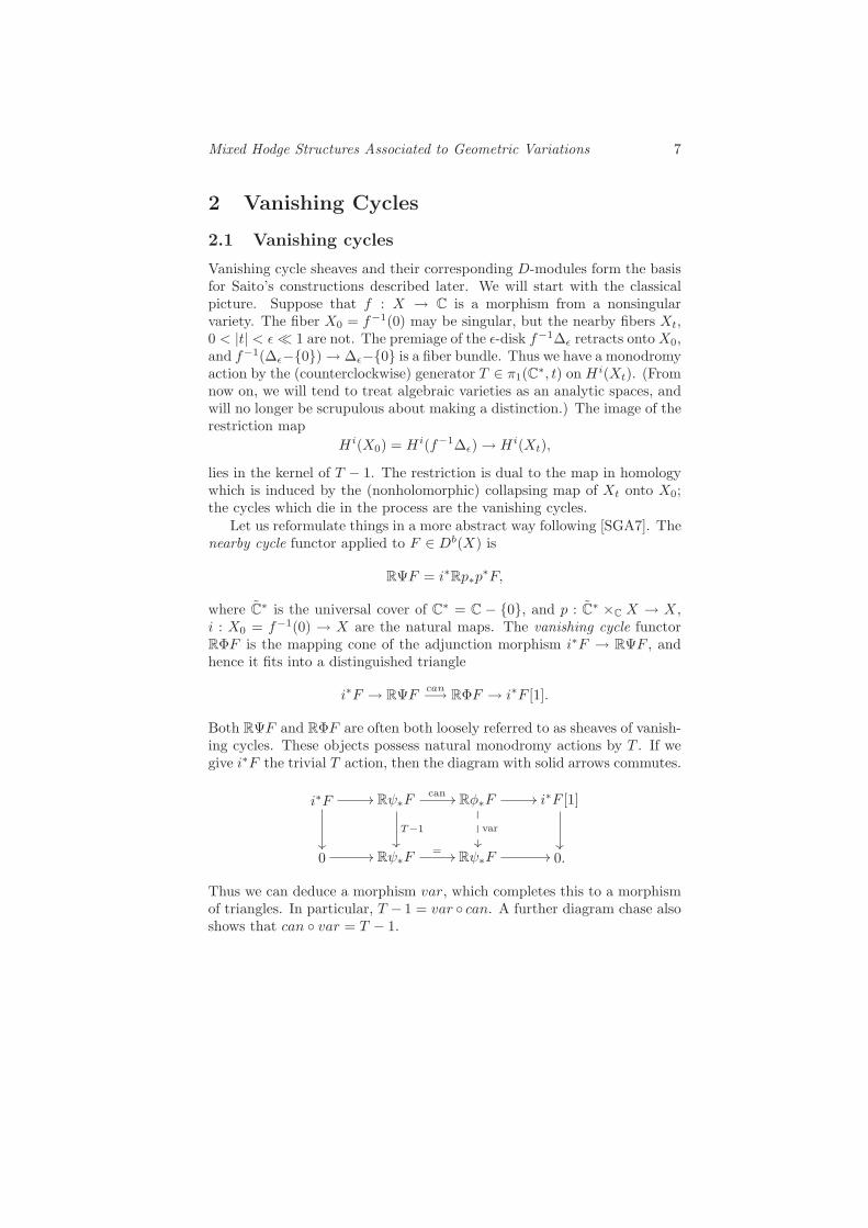
Both R&F and R'F are often both loosely referred to as sheaves of vanish-ing cycles. These objects possess natural monodromy actions by T . If wegive i"F the trivial T action, then the diagram with solid arrows commutes.
i"F !!
""
R&"Fcan
!!
T!1
""
R'"F !!
var
""!
!
!
i"F [1]
""
0 !! R&"F=
!! R&"F !! 0.
Thus we can deduce a morphism var, which completes this to a morphismof triangles. In particular, T - 1 = var 0 can. A further diagram chase alsoshows that can 0 var = T - 1.

8 Donu Arapura
Given p # X0, let B" be an $-ball in X centered at p. Then f!1(t)1B"
is the so called Milnor fiber. The stalks
Hi(R&Q)p = Hi(f!1(t) 1 B", Q)
Hi(R'Q)p = Hi(f!1(t) 1 B", Q)
give the (reduced) cohomology of the Milnor fiber. And
Hi(X0, R&Q) = Hi(f!1(t), Q)
is, as the terminology suggests, the cohomology of the nearby fiber. Wehave a long exact sequence
. . . Hi(X0, Q) % Hi(Xt, Q)can-% Hi(X0, R'Q) % . . . .
The following is a key ingredient in the whole story [BBD, Br]:
Theorem 2.1 (Gabber) If L is perverse, then so are R&L[-1] andR'L[-1].
We set p&fL = p&L = R&L[-1] and p'fL = p'L = R'L[-1].
2.2 Perverse Sheaves on a polydisk
Let % be a disk with the standard coordinate function t, and inclusionj : % - {0} = %" % %. Fix t0 # %". Consider a perverse sheaf F on %which is locally constant on %". Then we can form the diagram
p&tFcan
!! p'tFvar##
Note that the objects in the diagram are perverse sheaves on {0} i.e. vectorspaces. The space on the left is nothing but the stalk of F at t0. The spaceon the right can also be made concrete in various cases given below. Observethat since T = I + var 0 can is the monodromy of F |!! , it is invertible.This leads to the following elementary description of the category due toDeligne and Verdier (c.f. [V, §4]).
Proposition 2.2 The category of perverse sheaves on the disk % which arelocally constant on %" is equivalent to the category of quivers of the form
&c
!!
'v##
(i.e. finite dimensional vector spaces ',& with maps as indicated) such thatI + v 0 c is invertible.

Mixed Hodge Structures Associated to Geometric Variations 9
It is instructive to consider some basic examples. We see immediatelythat
0!!
V##
corresponds to the sky scraper sheaf V0. Now suppose that T is an auto-morphism of a vector space V . This determines a local system L on %".Then the perverse sheaf j"L[1] corresponds to
VT!I
!!
im(T - I)v##
where v is the inclusion. The perverse sheaf Rj"L[1] corresponds to
VT!I
!!
Vid
##
The above description can be extended to polydisks %n [GGM]. Forsimplicity, we spell this out only for n = 2. Let ti denote the coordi-nates. Then we can attach to any perverse sheaf F , four vector spacesV11 = p&t1
p&t2F , V12 = p't1p&t2F . . . along with maps induced by can and
var. The set of these maps have additional commutivity and invertibilityconstraints, such as cant1 0 cant2 = cant2 0 cant1 etcetera.
Theorem 2.3 The category of perverse sheaves on the polydisk %2 whichare constructible for the stratification %2 2 % / {0} ) {0} /% 2 {(0, 0)}is equivalent to the category of commutative quivers of the form
V11
c!!
c
""
V12v##
c
""
V21
v
$$
c!!
V22v##
v
$$
for which I + v 0 c is invertible.
It will be useful to characterize the subset of intersection cohomologycomplexes among all the perverse ones. On % these are either sky scrapersheaves V0 in which case ' = ker(v), or sheaves of the form j"L[1] for which' = im(c). On %2 (and more generally), we have:
Lemma 2.4 A quiver corresponds to a direct sum of intersection cohomol-ogy complexes if and only if
Vij = im(c) 3 ker(v)

10 Donu Arapura
holds for every subdiagram
Vi"j"
c!!
Vijv##
2.3 Kashiwara-Malgrange filtration
In this section, we give the D-module analogue of vanishing cycles (c.f. [PS,§14.2], [S1, §3]). But first we start with a motivating example.
Exercise 2.5 Let Y = C with coordinate t. Let M =(
m OnC[t!m] with
the standard basis ei. We make this into a DC-module by letting !t acton the left through the singular connection $ = d
dt + Adtt , where A is a
complex matrix with rational eigenvalues. There is no loss of generalityin assuming that A is in Jordan canonical form. For each ( # Q, defineV#M " M to be the C-span of {tmei | m # Z,m + aii 4 -(} where ei isthe standard basis of M . The following properties are easy to check:
1. The filtration is exhaustive and left continuous: )V#M = M andV#+"M = V#M for 0 < $ ( 1.
2. !tV#M " V#+1M , and tV#M " V#!1M .
3. The associated graded
GrV# M = V#M/V#!"M =
"
{i|#+aii%Z}
Ct!#!aiiei
is isomorphic to the -( generalized eigenspace of A. Moreover, theaction of t!t on this is space is identical to the action of A.
(3) implies that the set of indices where V#M jumps is discrete. (Such afiltration is called discrete.)
Let f : X % C be a holomorphic function, and let i : X % X / C = Ybe the inclusion of the graph. Let t be the coordinate on C, and let
V0DY = DX&{0}-module generated by {ti!jt | i 4 j}
This is the subring of di!erential operators preserving the ideal (t). LetM be a regular holonomic DX -module. It is called quasiunipotent alongX0 = f!1(0) if p&f (DR(M)) is quasiunipotent with respect to the actionof T # %1(C"). Set M = i+M .
Theorem 2.6 (Kashiwara, Malgrange) There exists at most one filtra-tion V•M on M indexed by Q, such that

Mixed Hodge Structures Associated to Geometric Variations 11
1. The filtration is exhaustive, discrete and left continuous.
2. Each V#M is a coherent V0DY -submodule.
3. !tV#M " V#+1M , and tV#M " V#!1M with equality for ( < 0.
4. GrV# M is a generalized eigenspace of t!t with eigenvalue -(.
If M is quasiunipotent along X0, then V•M exists.
The module M rather than M is used to avoid problems caused by thesingularities of f . When f is smooth, as in Example 2.5, we can and usuallywill construct the V -filtration directly on M .
Given a perverse sheaf L and ) # C, let p&f,$L and p'f,$L be thegeneralized )-eigensheaves of p&fL and p'fL under the T -action. The mapscan and var respect this decomposition into eigensheaves. It is technicallyconvenient at this point to define a modification V ar of var such thatcan0V ar and V ar0can equals N = 1
2%'!1
log Tu, where Tu is the unipotent
part of T in the multiplicative Jordan decomposition. After observing thaton each eigensheaf
log Tu =1
)N ( - 1
2(1
)N ()2 + · · ·
where N ( = T - ), a formula for V ar is easily found by setting
Var = a0var + a1var 0 N ( + a2var 0 (N ()2 + · · · ,
and solving for the coe"cients.
Exercise 2.7 Continuing with Example 2.5. Let L = DR(M). Thenp&tL = ker e"$, where t = e(#) = exp(2%
5-1#). A basis for this is
given by the columns of the fundamental solution of e"$ = 0 which is z =exp(-2%
5-1A#). This has monodromy given by T = exp(-2%
5-1A).
Then GrV# M is the -( generalized eigenspace of A, and this is isomorphic
to the ) generalized eigenspace of T where ) = e(().
Exercise 2.8 In the previous example, when n = 1, A = 0, the perversesheaf corresponding to M is L = Rj"CC! . We can see that GrV
1 M = Ct!1 +=p'tL. For the submodule OC , M , DR(O) = C and GrV
1 O = 0 += p'tC.
Theorem 2.9 (Kashiwara, Malgrange) Suppose that L = DR(M). Let( # Q and ) = e((). Then
DR(GrV# M) =
)
p&f,$L if ( # [0, 1)p'f,$L if ( # (0, 1]
The endomorphisms t!t + (, !t, t on the left corresponds to N, can, V arrespectively, on the right.

12 Donu Arapura
A proof is given in [S1, §3.4]. Note that some care is needed in comparingformulas here and in [loc. cit.]. There are shifts in indices according towhether one is working with left or right D-modules, and decreasing orincreasing V -filtrations.
3 Pre-Saito Hodge Theory
3.1 Hodge structures
A (rational) pure Hodge structure of weight m # Z consists of a finitedimensional vector space HQ with a bigrading
H = HQ & C ="
p+q=m
Hpq
satisfying Hpq = Hqp. Such structures arise naturally from the cohomologyof compact Kahler manifolds. For smooth projective varieties, we havefurther constraints namely the existence of a polarization on its cohomology.A polarization on a weight m Hodge structure H is quadratic form Q onHQ satisfying the Hodge-Riemann relations:
Q(u, v) = (-1)mQ(v, u) (3.1)
Q(Hpq,Hp"q"
) = 0, unless p = q(, q = p( (3.2)5-1
p!qQ(u, u) > 0, for u # Hpq, u 6= 0 (3.3)
Given a Hodge structure of weight m, its Hodge filtration is the decreas-ing filtration
F pH ="
p")p
Hp",m!p"
The decomposition can be recovered from the filtration by
Hpq = F p 1 F q
Deligne extended Hodge theory to singular varieties. The key defini-tion is that of a mixed Hodge structure. This consists of a bifiltered vec-tor space (H,F,W ), with (H,W ) defined over Q, such that F induces apure Hodge structure of weight k on GrW
k H. Note that by tradition F •
is a decreasing filtration denoted with superscripts, while W• is increasing.Whenever necessary, we can interchange increasing and decreasing filtra-tions by F• = F!•. A pure Hodge structure of weight k can be regarded asa mixed Hodge structure such that GrW
k H = H. A mixed Hodge structureis polarizable if each GrW
k H admits a polarization. Mixed Hodge structures

Mixed Hodge Structures Associated to Geometric Variations 13
form a category in the obvious way. Morphisms are rational linear mapspreserving filtrations.
Theorem 3.1 (Deligne [De3]) The category of mixed Hodge structuresis a Q-linear abelian category with tensor product. The functors GrW
k andGrp
F are exact.
The main examples are provided by:
Theorem 3.2 (Deligne [De3]) The singular rational cohomology of acomplex algebraic variety carries a canonical polarizable mixed Hodge struc-ture.
Finally, recall that there is a unique one dimensional pure Hodge struc-ture Q(j) of weight -2j up to isomorphism. By convention, the lattice istaken to be (2%
5-1)jQ. The jth Tate twist H(j) = H & Q(j).
3.2 Variations of Hodge structures
Gri"ths introduced the notion a variation of Hodge structure to describethe cohomology of family of varieties y '% Hm(Xy), where f : X % Y is asmooth projective map. A variation of Hodge structure of weight m on acomplex manifold Y consists of the following data [Sc]:
• A locally constant sheaf L of Q vector spaces with finite dimensionalstalks.
• A vector bundle with an integrable connection (E,$) plus an isomor-phism DR(E) += L & C[dim Y ].
• A filtration F • of E by subbundles satisfying Gri"ths’ transversality:$(F p) " F p!1.
• The data induces a pure Hodge structure of weight m on each of thestalks Ly.
A polarization on a variation of Hodge structure is a flat pairing Q : L/L %Q inducing polarizations on the stalks. The main example is:
Exercise 3.3 If f : X % Y is smooth and projective, L = Rmf"Qunderlies a polarizable variation of Hodge structure of weight m. E =Rmf"$•
X/Y+= OY &L is the associated vector bundle with its Gauss-Manin
connection and Hodge filtration F p = Rmf"$)pX/Y .
The next class of examples is of fundamental importance.

14 Donu Arapura
Exercise 3.4 An n dimensional nilpotent orbit of weight m consists of
• a filtered complex vector space (H,F ) where H carries a real struc-ture,
• a real form Q on H satisfying the first two Hodge-Riemman relations,
• n mutually commutating nilpotent infinitesimal isometries Ni of (H,Q)such that NiF p " F p!1,
• there exist c > 0 such that for Im(zi) > c, (H, exp(#
ziNi)F,Q) is apolarized Hodge structure of weight m
Then the filtered polarized bundle with fibre (H, exp(#
ziNi)F,Q) de-scends to a real holomorphic variation of Hodge structure on a puncturedpolydisk (% - {0})n. The monodromy around the ith axis is preciselyexp(Ni).
Schmid [Sc, §4] showed that any polarized variation of Hodge structureon a punctured polydisk can be very well approximated by a nilpotent orbitwith the same asymptotic behaviour. Thus the local study of a variationof Hodge structure can be reduced to nilpotent orbits. When the localmonodromies are unipotent (which can always be achieved by passing toa branched covering), an approximating nilpotent orbit (H,F,Ni) can beconstructed in canonical fashion: H is the fibre of the Deligne’s canonicalextension [De2] at 0. The Hodge bundles extend to subbundles of thecanonical extension and F is their fibre at 0. Ni are the logarithms of localmonodromy.
The key analytic fact which makes the rest of the story possible is thefollowing theorem (originally proved by Zucker [Z] for curves).
Theorem 3.5 [Cattani-Kaplan-Schmid [CKS], Kashiwara-Kawai[KK]] Let X be the complement of a divisor with normal crossings in acompact Kahler manifold. Then intersection cohomology with coe!cientsin a polarized variation of Hodge structure on X is isomorphic to L2 coho-mology for a suitable complete Kahler metric on the X.
It should be noted that in contrast to the compact case, L2 cohomologyof a noncompact manifold is highly sensitive to the choice the metric, andthat it could be infinite dimensional. Here the metric is chosen to be asymp-totic to a Poincare metric along transverse slices to the boundary divisor.From the theorem, it follows that L2 cohomology is finite dimensional inthis case. When combined with the Kahler identities, we get
Corollary 3.6 Intersection cohomology IHi(X,L) = Hi!n(X, j!"L[n])with coe!cients in a polarized variation of Hodge structure of weight kcarries a natural pure Hodge structure of weight i + k.

Mixed Hodge Structures Associated to Geometric Variations 15
3.3 Monodromy filtration
We start with a result in linear algebra which is crucial for later develop-ments.
Proposition 3.7 (Jacobson, Morosov) Fix an integer m. Let N be anilpotent endomorphism of a finite dimensional vector space E over a fieldof characteristic 0. Then the there is a unique filtration
0 " Mm!l , · · ·Mm " · · · " Mm+l = E
called the monodromy filtration on E centered at m (in symbols M =M(N)[m]), characterized by following properties:
1. N(Mk) " Mk!2
2. Nk induces an isomorphism GrMm+k(E) += GrM
m!k(E)
In applications N comes from monodromy, which explains the termi-nology. The attribution is a bit misleading since it is really a corollary ofthe Jacobson- Morosov theorem. However, it can be given an elementarylinear algebra proof (c.f. [Sc, 6.4]), which makes it clear that it appliesto any artinian Q or C-linear abelian category such as the categories ofperverse sheaves or regular holonomic modules. The last part of the propo-sition is reminiscent of the hard Lefschetz theorem. There is an analogousdecomposition into primitive parts:
Corollary 3.8
GrMk (E) =
"
i
N iPGrMk+2i(E)
where
PGrMm+k(E) = ker[Nk+1 : GrM
m+k(E) % GrMm!k!2(E)]
Returning to Hodge theory, M gives the weight filtration of Schmid’slimit mixed Hodge structure [Sc], which is a natural mixed Hodge structureon the space of nearby cycles. We combine this with the converse statementof Cattani and Kaplan [CK].
Theorem 3.9 (Schmid, Cattani-Kaplan) Suppose that (H,F,Ni, Q) isa collection satisfying all but the last condition of Example 3.4. Then thisis a nilpotent orbit of weight m if and only all of the following hold:
1. M = M(#
Ni)[m] = M(#
tiNi)[m] for any ti > 0.
2. (H,M) is a real mixed Hodge structure.

16 Donu Arapura
3. This structure is polarizable; more specifically, the form Q(·, Nk·)gives a polarization on the primitive Hodge structures PGrM
m+k(H).
Given a filtered vector space (V,W ) with nilpotent endomorphism Npreserving W , a relative monodromy filtration is a filtration M on V suchthat
• NMk " Mk!2
• M induces the monodromy filtration centered at k on GrWk V with
respect to N .
It is known that M is unique if it exists (c.f. [SZ]), although it need notexist in general. In geometric situations, the existence of relative weightfiltrations was first established by Deligne using *-adic methods.
3.4 Variations of mixed Hodge structures
A variation of mixed Hodge structure consists of:
• A locally constant sheaf L of Q vector spaces with finite dimensionalstalks.
• An ascending filtration W " L by locally constant subsheaves
• A vector bundle with an integrable connection (E,$) plus an isomor-phism DR(E) += L & C[dim Y ].
• A filtration F • of E by subbundles satisfying Gri"ths’ transversality:$(F p) " F p!1.
• (GrWm (L),OX & GrW
m (L), F •(OX & GrWm (L))) is a variation of pure
Hodge structure of weight m.
It follows that this data induces a mixed Hodge structure on each of thestalks Ly. Steenbrink and Zucker [SZ] showed that additional conditions arerequired to get a good theory. While these conditions are rather technical,they do hold in most natural examples.
A variation of mixed Hodge structure over a punctured disk %" is ad-missible if
• The pure variations GrWm (L) are polarizable.
• There exists a limit Hodge filtration limt*0 F pt compatible with the
one on GrWm (L) constructed by Schmid.
• There exist a relative monodromy filtration M on (E = Lt,W ) withrespect to the logarithm N of the unipotent part of monodromy.

Mixed Hodge Structures Associated to Geometric Variations 17
For a general base X the above conditions are required to hold for everyrestriction to a punctured disk [K1]. Note that pure polarizable variationsof Hodge structure are automatically admissible by [Sc]. A local modelfor admissible variations is provided by a mixed nilpotent orbit called aninfinitesimal mixed Hodge module in [K1]. This consists of:
• A bifiltered complex vector space (H,F,W ) with (H,W ) defined overR,
• commuting real nilpotent endomorphisms Ni satisfying NiF p " F p!1
and NiWk " Wk,
such that
• GrWk is a nilpotent orbit of weight k for some choice of form.
• The monodromy M filtration exists for any partial sum#
Nij, and
NijMk " Mk!2 holds for each ij .
With an obvious notion of morphism, mixed nilpotent orbits of a givendimension forms a category which turns out to be abelian [K1, 5.2.6].
4 Hodge Modules
4.1 Hodge modules on a curve
We are now ready to begin describing Saito’s category of Hodge modulesin a special case. We start with the category MFrh(DX , Q) whose objectsconsist of
• A perverse sheaf L over Q.
• A regular holonomic DX -module M with an isomorphism DR(M) +=L & C.
• A good filtration F on M .
Morphisms are compatible pairs of morphisms of (M,F ) and L. Varia-tions of Hodge structure give examples of such objects (note that Grif-fiths’ transversality !xi
Fp " Fp+1 is needed to verify (3)). The categoryMFrh(X, Q) is really too big to do Hodge theory, and Saito defines thesubcategory of (polarizable) Hodge modules which provides a good setting.The definition of this subcategory is extremely delicate, so as a warm upwe will give a direct description for Hodge modules on a smooth projectivecurve X (fixed for the remainder of this section).
Given an inclusion of a point i : {x} % X and a polarizable pure Hodgestructure (H,F,HQ) of weight k, the D-module pushforward i+H with the

18 Donu Arapura
filtration induced by F , together with the skyscraper sheaf HQ,x defines anobject of MFrh(X). Let us call these polarizable Hodge modules of type 0and weight k.
Given a polarizable variation of Hodge structure (E,F,L) of weight k-1over a Zariski open subset j : U % X, we define an object of MFrh(X) asfollows. The underlying perverse sheaf is j"L[1] which is the intersectioncohomology complex for L. Since (E,$) has regular singularities [Sc],we can extend it to a vector bundle with logarithmic connection on X –in many ways [De2]. The ambiguity depends on the eigenvalues of theresidues of the extension which are determined mod Z. For every half openinterval I of length 1, there is a unique extension EI with eigenvalues in I.Let M( =
(
I EI " j"E. This is a DX -module which corresponds to theperverse sheaf Rj"L[1]&C. Let M " M( be the sub DX -module generatedby E(!1,0]. This corresponds to what we want, namely j"L[1]. We filterthis by
FpE(!1,0] = j"FpE 1 E(!1,0]
FpM =!
i
FiDXFp!iE(!1,0].
Since the monodromy is quasi-unipotent [Sc, 4.5], the V -filtration exists forgeneral reasons. However, in this case we can realize this explicitly by
V#M = E[!#,!#+1).
This is essentially how we described it in Example 2.5. From this it followsthat
Fp 1 V#M = j"FpE 1 E[!#,!#+1)
for ( < 1. The collection (M, F•M, j"L[1]) defines an object of MFrh(X)that we call a polarizable Hodge module of type 1 of weight k. A polarizableHodge module of weight k is a finite direct sum of objects of these two types.Let MH(X, k)p denote the full subcategory of these.
Theorem 4.1 MH(X, k)p is abelian and semisimple.
In outline, the proof can be reduced to the following observations. Weclaim that there are no nonzero morphisms between objects of type 0 andtype 1. To see this, we can replace X by a disk and assume that x andU above correspond to 0 and %" respectively. Then by Lemma 2.2, theperverse sheaves of type 0 and 1 correspond to the quivers
0!!
'##
&onto
!!
'1!1
##

Mixed Hodge Structures Associated to Geometric Variations 19
and the claim follows. We are thus reduced to dealing with the typesseparately. For type 0 (respectively 1), we immediately reduce it the corre-sponding statements for the categories of polarizable Hodge structures (re-spectively variation of Hodge structures), where it is standard. In essencethe polarizations allow one to take orthogonal complements, and henceconclude semisimplicity.
Theorem 4.2 If M # MH(X, k)p, then its cohomology Hi(M) carries apure Hodge structure of weight k.
Proof Since MH(X, k)p is semisimple, we can assume that M is simple.Then either M is supported at point or it is of type 1. In the first case,H0(M) = M is already a Hodge structure of weight k by definition, and thehigher cohomologies vanish. In the second case, we appeal to Theorem 3.5or just the special case due to Zucker.
!
We end with a local analysis of Hodge modules. By a Hodge quiver wemean a diagram
&c
!!
'v##
where & and ' are mixed Hodge structures, c is morphism and v is amorphism ' % &(-1) to the Tate twist, and such that the compositionsc 0 v, v 0 c (both denoted by N) are nilpotent. Actually, we will need toadd a bit more structure, but we can hold o! on this for the moment. Wecan encode the local structure of a Hodge module by a Hodge quiver. Amodule of type 0 and weight k corresponds to the quiver
0!!
'##
where ' is pure of weight k.Next, consider the type 1 modules. We wish to associate a Hodge quiver
to a polarizable variation of Hodge structure (E,F,L) of weight k - 1 over%". First suppose that the monodromy is unipotent. Then let & = p&tL[1]with its limit mixed Hodge structure i.e. the mixed Hodge structure on
E(!1,0]0 with Hodge filtration given by F •E(!1,0]
0 and weight filtration W =M(N)[k - 1]. Set ' = im(N) = &/ker(N) with its induced mixed Hodgestructure. Then
&N
!!
'id
##
gives the corresponding Hodge quiver. The Hodge quivers arising from thisconstruction are quite special in that (&, F,N) and (', F,N) are nilpotentorbits of weight k - 1 and k respectively by [KK, 2.1.5].

20 Donu Arapura
In general, the monodromy is quasi-unipotent. Thus for some r, thepullback of L along % : t '% tr is unipotent. So we can repeat the previousconstruction. But now the Galois group Z/rZ will act on everything, and itwill be necessary to include this action as part of the structure of a Hodgequiver so as not to lose any information. This can be understood directlywithout doing a base change. The decomposition of & = p&tL[1] += p&t%"Linto a sum isotypic Z/rZ-modules can be identified with the decompostioninto generalized eigenspaces for the T -action. By Theorem 2.9, we canrealize this decomposition by
& ="
0+#<1
GrV# M.
For the Hodge filtration, we use the induced filtration
F •GrV M ="
#
F • 1 V#MF • 1 V#!"M
="
#
j"F • 1 E[!#,!#+1)
j"F • 1 E(!#,!#+1]
where M = D!E(!1,0] is defined as above. For N we take the logarithmof the unipotent part of T under the multiplicative Jordan decomposition.Then (&, F,N) is a nilpotent orbit of weight k - 1, which determines amixed Hodge structure. ' and the rest of the diagram is defined as before.In this case, we include the grading of &,' by eigenspaces as part of thestructure of a Hodge quiver. In this way, we can recover the full monodromyT rather than just N .
In summary, every polarizable Hodge module on the disk gives rise to aHodge quiver. This yields a functor which is necessarily faithful, since thequiver determines the underlying perverse sheaf. This can be made intoa full embedding by adding more structure to a Hodge quiver (namely, achoice of a variation of Hodge structure on %", . . .). However, this will notbe necessary for our purposes.
4.2 Hodge modules: overview
In the next section, we will define the full subcategories MH(X,n) "MFrh(X, Q) of Hodge modules of weight n # Z in general. Since this israther technical, we start by explaining the main results. Aside from Saito’soriginal papers [S1, S3], further explanations can be found in Brylinski-Zucker [BZ], Peters-Steenbrink [PS] and Sabbah [Sb]. The constructionand basic properties of the categories are contained in [S1, §5.1-5.2]:
Theorem 4.3 (Saito) MH(X,n) is abelian, and its objects possess strictsupport decompositions, i.e. that the maximal sub/quotient module with

Mixed Hodge Structures Associated to Geometric Variations 21
support in a given Z " X can be split o" as a direct summand. There is anabelian subcategory MH(X,n)p of polarizable objects which is semisimple.
We essentially checked these properties for polarizable Hodge moduleson curves in section 4.1. They have strict support decompositions by theway we defined them. Let MHZ(X,n) " MH(X,n) denote the subcate-gory of Hodge modules with strict support in Z, i.e. that all sub/quotientmodules have support exactly Z. The main examples are provided by thefollowing.
Theorem 4.4 (Saito) Any weight m polarizable variation of Hodge struc-ture (L, . . .) over an open subset of a closed subset
Uj% Z
i% X
can be extended to a polarizable Hodge module in MHZ(X,n)p"MH(X,n)p
with n = m + dimZ. The underlying perverse sheaf of the extension is theassociated intersection cohomology complex i"j!"L[dimU ]. All simple ob-jects of MH(X,n)p are of this form.
Proof This follows from theorem 3.21 of the second paper [S3] along withthe discussion leading up to it. A sketch can also be found in [S2].
!
Tate twists M '% M(j) can be defined in this setting and are functorsMH(X,n) % MH(X,n - 2j). Given a morphism f : X % Y and L #Perv(X), we can define perverse direct images by pRf i
"L = pHi(Rf"L).This operation extends to Hodge modules. If f is smooth and projectiveand (M,F,L) # MH(X), the direct image is pRf i
"L with the associatedfiltered D-module given by a Gauss-Manin construction:
(Rif"($•X/Y &OX
M), im[Rif"($•X/Y &OX
Fp+•M)])
When applied to (OX , QX [dimX]) with trivial filtration, we recover thevariation of Hodge structure of example 3.3 (after adjusting notation).
Theorem 4.5 (Saito [S1, 5.3.1]) Let f : X % Y be a projective mor-phism with a relatively ample line bundle *. If M = (M,F,L) # MH(X,n)is polarizable, then
pRif"M # MH(Y, n + i)
Moreover, a hard Lefschetz theorem holds:
*j) : pR!jf"M += pRjf"M(j)

22 Donu Arapura
Corollary 4.6 Given a polarizable variation of Hodge structure definedon an open subset of X, its intersection cohomology carries a pure Hodgestructure. This cohomology satisfies the Hard Lefschetz theorem.
The last statement was originally obtained in the geometric case in[BBD]. The above results yield a Hodge theoretic proof of the decomposi-tion theorem of [loc. cit.]
Corollary 4.7 With assumptions of the theorem Rf"Q decomposes into adirect sum of shifts of intersection cohomology complexes.
4.3 Hodge modules: conclusion
We now give the precise definition of Hodge modules. This is given byinduction on dimension of the support. This inductive process is handledvia vanishing cycles. We start by explaining how to extend the constructionto MFrh(X, Q). Given a morphism f : X % C, and a DX -module, M , weintroduced the Kashiwara-Malgrange filtration V on M in Section 2.3. Nowsuppose that we have a good filtration F on M . The pair (M,F ) is said tobe be quasi-unipotent and regular along f!1(0) if V exists and if
1. t(FpV#M) = FpV#!1M for ( < 1.
2. !t(FpGrV# M) = Fp+1GrV
#+1M for ( 4 0.
hold along with certain finiteness properties that we will not spell out.Saito [S1, 3.4.12] has shown Theorem 2.9 holds assuming only the existenceof such a filtration F . As for examples, note that a variation of Hodgestructure on a disk can be seen to satisfy these conditions using the formulasof Section 4.1 and [S1, 3.2.2]. Also any D-module which is quasi-unipotentand regular in the usual sense admits a filtration F as above.
We extend the functors ' and & to MFrh(X, Q) by
&f,e(#)(M,F,L) = (GrV# (M), F [1], p&f,e(#)L), 0 . ( < 1
'f,e(#)(M,F,L) = (GrV#+1(M), F, p'f,e(#)L), 0 . ( < 1
&f ="
&f,$, 'f ="
'f,$
Where F on the right denotes the induced filtration. Thanks to the shiftin F , !t and t induce morphisms
can : &f,e(#)(M,F,L) % 'f,e(#)(M,F,L)
var : 'f,e(#)(M,F,L) % &f,e(#)(M,F,L)
respectively.

Mixed Hodge Structures Associated to Geometric Variations 23
We are ready to give the inductive definition of MH(X,n). The ele-mentary definition for curves given earlier will turn out to be equivalent.Define X '% MH(X,n) to be the smallest collection of full subcategoriesof MFrh(X, Q) satisfying:
(MH1) If (M,F,L) # MFrh(X, Q) has zero dimensional support, then it liesin MH(X,n) i! its stalks are Hodge structures of weight n.
(MH2) If (M,F,L) # MHS(X,n) and f : U % C is a general morphismfrom a Zariski open U " X, then
(a) (M,F )|U is quasi-unipotent and regular with respect to f .
(b) (M,F,L)|U decomposes into a direct sum of a module supportedin f!1(0) and a module for which no sub or quotient module issupported in f!1(0).
(c) If W is the monodromy filtration of &f (M,F,L)|U (with re-spect to the log of the unipotent part of monodromy) centeredat n - 1, then GrW
i &f (M,F,L)|U # MH(U, i). Likewise forGrW
i 'f,1(M,F,L) with W centered at n.
This is a lot to absorb, so let us make few remarks about the definition.
• If f!1(0) is in general position with respect to suppM , the dimensionof the support drops after applying the functors ' and &. Thus thisis an inductive definition.
• The somewhat technical condition (b) ensures that Hodge modulesadmit strict support decompositions. The condition can be rephrasedas saying that (M,F,L) splits as a sum of the image of can and thekernel of var. A refinement of Lemma 2.4 shows that L will thendecompose into a direct sum of intersection cohomology complexes.This is ultimately needed to be able to invoke Theorem 3.5 when thetime comes to construct a Hodge structure on cohomology.
• Although MFrh(X, Q) is not an abelian category, the category ofcompatible pairs consisting of a D-module and perverse sheaf is. Thuswe do get a W filtration for &f (M,F,L)|U in (c) by Proposition 3.7by first suppressing F , and then using the induced filtration.
There is a notion of polarization in this setting. Given (M,F,L) #MHZ(X,n), a polarization is a pairing S : L & L % QX [2 dim X](-n)satisfying certain axioms. The key conditions are again inductive. WhenZ is a point, S should correspond to a polarization on the Hodge structureat the stalk in the usual sense. In general, given a (germ of a) functionf : Z % C which is not identically zero, S should induce a polarization on

24 Donu Arapura
the nearby cycles GrW• &fL (using the same recipe as in Theorem 3.9 (3)).
Once all the definitions are in place, the proofs of the theorems involve arather elaborate induction on dimension of supports.
In order to get a better sense of what Hodge modules look like, we extendthe local description given in §4.1 to the polydisk %2. We assume thatthe underlying perverse sheaves satisfying the assumptions of theorem 2.3.Then using a vanishing cycle construction refining the one used earlier, sucha polarizable Hodge module gives rise to a two dimensional Hodge quiver.This is a commutative diagram of Q2-graded mixed Hodge structures
H11
c!!
c
""
H12v##
c
""
H21
v
$$
c!!
H22v##
v
$$
such that the maps labeled c and v are required to satisfy the same condi-tions as in §4.1. In particular, compositions c0 v, v 0 v are nilpotent. Thesenilpotent transformations are denoted by N1 for horizontal arrows, and N2
for vertical.Given a Hodge module M of weight k, H11 = &t2&t2M # MFrh(pt, Q)
etcetera are filtered vector spaces with a Q2-grading by eigenspaces. Thesefiltrations are used as the Hodge filtrations. The weight filtration is givenby the shifted monodromy filtration with respect to N = N1 + N2, whereNi are the logarithms of the unipotent parts of monodromy around theaxes. The shifts are indicated in the diagram below
k - 2!!
""
k - 1##
""
k - 1
$$
!!
k##
$$(4.1)
These quivers are quite special. A Hodge quiver is pure of weight k if theconditions of Lemma 2.4 hold, and if each (Hij , F,W,N1, N2) arises froma pure nilpotent orbit of weight indicated indicated in (4.1). With thisdescription in hand, we can verify a local version of Theorem 4.4. Given apolarizable variation of Hodge structure L of weight k - 2 on (% - {0})2corresponding to a nilpotent orbit (H,F,N1, N2), we can construct theHodge quiver
HN1
!!
N2
""
N1Hid##
N2
""
N2H
id
$$
N1!!
N1N2Hid##
id
$$

Mixed Hodge Structures Associated to Geometric Variations 25
where H is equipped with the monodromy filtration W (N1 + N2) on theupper left. The remaining vertices are given the mixed Hodge structuresinduced on the images of this. The fact that these vertices correspondto nilpotent orbits of the correct weight follows from [CKS, 1.16] or [KK,2.1.5]. Note that j!"L[2] is the perverse sheaf corresponding to this diagram.The details can be found in [S3, §3].
4.4 Mixed Hodge modules
Saito has given an extension of the previous theory by defining the notionof mixed Hodge module. We will define a pre-mixed Hodge module on X toconsist of
• A perverse sheaf L defined over Q, together with a filtration W of Lby perverse subsheaves.
• A regular holonomic DX -module M with a filtration WM whichcorresponds to (L & C,W & C) under Riemann-Hilbert.
• A good filtration F on M.
These objects form a category, and Saito defines the subcategory ofmixed Hodge modules MHM(X) by a rather delicate induction. The keypoints are that for (M, F, L,W ) to be in MHM(X), he requires
• The associated graded objects GrWk (M, F, L) yield polarizable Hodge
modules of weight k.
• For any (germ of a) function f on X, the relative monodromy filtra-tion M (resp. M () for &f (M, F, L) (resp. 'f,1(M, F, L)) with respectto W exists.
• The pre-mixed Hodge modules
(&f (M, F, L),M) and ('f,1(M, F, L),M ()
are in fact mixed Hodge modules on f!1(0).
This is not a complete list of all the conditions. Saito also requires thatmixed Hodge modules should be extendible across divisors in a sense wewill not attempt to make precise. (To avoid confusion, we are using the def-inition of MHM given in section 4 of [S3], where polarizability is assumed.)The main properties are summarized below:

26 Donu Arapura
Theorem 4.8 (Saito)
1. MHM(X) is abelian, and it contains each MH(X,n)p as a fullabelian subcategory.
2. MHM(point) is the category of polarizable mixed Hodge structures.
3. If U " X is open, then any admissible variation of mixed Hodgestructure on U extends to an object in MHM(X).
Proof For the first statement see [S3, 4.2.3], and [S3, 3.9,3.27] for theremaining statements.
!
Finally, we have:
Theorem 4.9 (Saito [S3, thm 0.1]) There is a realization functor of tri-angulated categories
real : DbMHM(X) % Dbconstr(X, Q)
and functors
pHi : DbMHM(X) % MHM(X)
Rf" : DbMHM(X) % DbMHM(Y )
Lf" : DbMHM(Y ) % DbMHM(X)
for each morphism f : X % Y , such that
pHi 0 real = real 0 pHi
real(Rf"M) = Rf"real(M)
real(Lf"N ) = Lf"real(M)
Similar statements hold for various other standard operations such as tensorproducts and cohomology with proper support.
Putting these results together yields Saito’s mixed Hodge structure:
Theorem 4.10 The cohomology of a smooth variety U with coe!cientsin an admissible variation of mixed Hodge structure L carries a canonicalmixed Hodge structure.
When the base is a curve, this was first proved by Steenbrink and Zucker[SZ].

Mixed Hodge Structures Associated to Geometric Variations 27
Proof L gives an object of MHM(U). Thus Hi(Rp"L) carries a mixedHodge structure, where p : U % pt is the projection to a point.
!
We extend the local description of perverse sheaves and Hodge modulesto mixed Hodge modules. A one dimensional filtered Hodge quiver is adiagram
&c
!!
'v##
where & and ' are filtered Q-graded mixed Hodge structures, c and v : ' %&(-1) are morphisms and the compositions c0v, v 0 c (both denoted by N)are nilpotent. So each object &,' is equipped with 3 filtrations F,M,W ,where M denotes the weight filtration. For a filtered Hodge quiver to arisefrom a mixed Hodge module, we require that
• GrkW is pure of weight k.
• (&, F,W,N) and (', F,W,N) are mixed nilpotent orbits with M therelative monodromy filtration.
We call these admissibility conditions. This extends to polydisks in astraightforward manner.
4.5 Explicit construction
We will give a bit more detail on the construction of the mixed Hodgestructure in Theorem 4.10. For a di!erent perspective see [E]. Let U be asmooth n dimensional variety. We can choose a smooth compactificationj : U % X such that D = X - U is a divisor with normal crossings.Fix an admissible variation of mixed Hodge structure (L,W,E, F,$) on U .Extend (E,$) to a vector bundle EI with a logarithmic connection suchthat the eigenvalues of its residues lie in I as in Section 4.1 Let E = E(!1,0]
and M =(
I EI " j"E. Then M is a DX -module which corresponds tothe perverse sheaf Rj"L[n] & C. Filter this by
FpM =!
i
FiDXFp!iE
Then:
Theorem 4.11 There exists compatible filtrations W on Rj"L[n] and Mextending W over U such that (Rj"L[n], W ,M, F ) becomes a mixed Hodgemodule.
28 Donu Arapura
We describe W when n = dimX . 2. We start with the case of n =1, which is essentially due to Steenbrink and Zucker [SZ]. It su"ces toconstruct W locally near any point of p # D. Choose a coordinate disk %at p. The perverse sheaf Rj"L[1] corresponds to the quiver
&N
!!
&id
## (4.2)
where & = &tL and N is the logarithm of unipotent part of monodromy atp. We make this into an admissible filtered Hodge quiver by replacing & onthe left with the mixed nilpotent orbit (H,F •H,W•H,N), where we cantake H = E0 when the monodromy is unipotent, and H = 3GrV
# (D!E) ingeneral. On the right, we keep (H,F •H,N) but replace W with
(N"W )k!1 := NWk + Mk 1 Wk!1 (4.3)
where M is the relative monodromy filtration of (H,W ). This is a mixednilpotent orbit by [K1, 5.5.4]. Then define the filtration Wk of (4.2) by
Wk!1
N!!
(N"W )k!2id
##
The key point is that GrWk is pure of weight k, because it is a sum of
GrWk!1
N!!
NGrWk!1id
##
and
0!!
GrMk!2(Wk!2/NWk!2)(-1)##
both pure of weight k. A proof can be extracted from [SZ, pp 514-516] or[K1]. Since we have an equivalence of categories between perverse sheaveson % and quivers, W above determines a filtration of Rj"L[1] by perversesubsheaves.
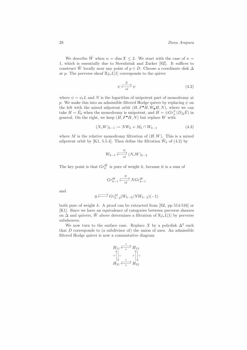
We now turn to the surface case. Replace X by a polydisk %2 suchthat D corresponds to (a subdivisor of) the union of axes. An admissiblefiltered Hodge quiver is now a commutative diagram
H11
c!!
c
""
H12v##
c
""
H21
v
$$
c!!
H22v##
v
$$
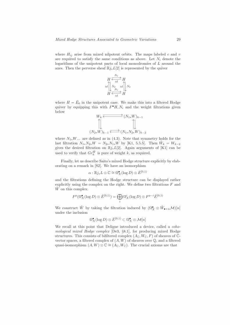
Mixed Hodge Structures Associated to Geometric Variations 29
where Hij arise from mixed nilpotent orbits. The maps labeled c and vare required to satisfy the same conditions as above. Let Ni denote thelogarithms of the unipotent parts of local monodromies of L around theaxes. Then the perverse sheaf Rj"L[2] is represented by the quiver
HN1
!!
N2
""
Hid
##
N2
""
H
id
$$
N1!!
Hid
##
id
$$
where H = E0 in the unipotent case. We make this into a filtered Hodgequiver by equipping this with F •H,Ni and the weight filtrations givenbelow
Wk!!
""
(N1"W )k!1##
""
(N2"W )k!1
$$
!!
(N1"N2"W )k!2##
$$
where N1"W ... are defined as in (4.3). Note that symmetry holds for thelast filtration N1"N2"W = N2"N1"W by [K1, 5.5.5]. Then Wk = Wk!2
gives the desired filtration on Rj"L[2]. Again arguments of [K1] can be
used to verify that GrWk is pure of weight k, as required.
Finally, let us describe Saito’s mixed Hodge structure explicitly by elab-orating on a remark in [S2]. We have an isomorphism
( : Rj"L & C += $•X(log D) & E[0,1)
and the filtrations defining the Hodge structure can be displayed ratherexplicitly using the complex on the right. We define two filtrations F andW on this complex.
F p($•X(log D) & E[0,1)) =
"
i
$iX(log D) & F p!iE[0,1)
We construct W by taking the filtration induced by ($•X & W•+nM)[n]
under the inclusion
$•X(log D) & E[0,1) , $•
X &M[n]
We recall at this point that Deligne introduced a device, called a coho-mological mixed Hodge complex [De3, §8.1], for producing mixed Hodgestructures. This consists of bifiltered complex (AC,WC, F ) of sheaves of C-vector spaces, a filtered complex of (A,W ) of sheaves over Q, and a filteredquasi-isomorphism (A,W ) & C += (AC,WC). The crucial axioms are that

30 Donu Arapura
• this datum should induce a pure weight i + k Hodge structure onHi(GrW
k A)
• the filtration induced by F on GrWk is strict, i.e. the map
Hi(F pGrWk A) % Hi(GrW
k A)
is injective.
Proposition 4.12 With these filtrations
(Rj"L, W ;$X(log D)• & E, W , F ;()
becomes a cohomological mixed Hodge complex.
To verify the above axioms, one observes that GrWk Rj"L decomposes
into a direct sum of intersection cohomology complexes associated to purevariations of Hodge structure of the correct weight. An appeal to Theo-rem 3.5 shows that Hi(GrW
k Rj"L) carries pure Hodge structures of weightk + i. Strictness follows from similar considerations.
From [De3, §8.1], we obtain
Corollary 4.13 The Hodge filtration is induced by F under the isomor-phism
Hi(U,L & C) += Hi($•X(log D) & E[0,1))
The weight filtration is given by
Wi+kHi(U,L & C) = Hi(X,Wk($•X(log D) & E[0,1))).
Finally, we remark that in the simplest case L = Q, W above coincideswith the filtration W defined by Deligne [De3, §3.1]; in particular, Saito’sHodge structure coincides with Deligne’s in this case.
5 Comparison
From now on let f : X % Y be a smooth projective morphism of smoothquasiprojective varieties. We recall two results
Theorem 5.1 (Deligne [De1]) The Leray spectral sequence
Epq2 = Hp(Y,Rqf"Q) 7 Hp+q(X,Q)
degenerates. In particular Epq2
+= GrpLHp+q(X) for the associated “Leray
filtration” L.

Mixed Hodge Structures Associated to Geometric Variations 31
Theorem 5.2 ([A]) There exists varieties Yp and morphisms Yp % Ysuch that
LpHi(X, Q) = ker[Hi(X, Q) % Hi(Xp, Q)]
where Xp = f!1Yp.
It follows that each Lp is a filtration by sub mixed Hodge structures.When combined with Theorem 5.1, we get a mixed Hodge structure onHp(Y,Rqf"Q) which we will call the naive mixed Hodge structure. Onthe other hand, Rqf"Q carries a pure hence admissible variation of Hodgestructure, so we can apply Saito’s Theorem 4.10.
Theorem 5.3 The naive mixed Hodge structure on Hp(Y,Rqf"Q) coin-cides with Saito’s.
Proof Note that Rif"Q are local systems and hence perverse sheaves upto shift. More specifically,
Rif"Q = real(pHi!dim X+dim Y Rf"Q[dimX])[-dim Y ]
Deligne [De1] actually proved a stronger version of the above theorem whichimplies that
Rf"Q +="
i
Rif"Q[-i] (5.1)
(non canonically) in Dbconstr(X). By Theorem 4.5 and [loc. cit.], we have
the corresponding decomposition
Rf"Q[dimX] ="
i
pHi(Rf"Q[dimX])[-i]
in DbMHM(Y ). Note that the Leray filtration is induced by the truncationfiltration
LpHi(X, Q) = image[Hi(Y, #+i!pRf"Q % Hi(Y, Rf"Q)]
Under (5.1),
#+pRf"Q +="
i+p
Rif"Q[-i]
Therefore we have an isomorphism of mixed Hodge structures
Hi(X, Q) +="
p+q=i
Hp(Y,Rpf"Q)

32 Donu Arapura
where the right side is equipped with Saito’s mixed Hodge structure. Underthis isomorphism, Lp maps to
Hi!p(Rpf"Q) 3 Hi!p+1(Rp!1f"Q) 3 · · ·
The theorem now follows.!
As pointed out by the referee the theorem was also proved in [PS, 14.1.3]using compatibility of the perverse Leray spectral sequence with MHM .It can also be deduced from the decomposition theorem. A somewhatstronger statement would also follow from the remark [S3, 4.6.2] that onecan build a t-structure on DbMHM(X) which agrees with the standard oneon Db
constr(X). However, we decided not to include this since a detailedjustification for the remark was not given.
References
[A] D. Arapura, The Leray spectral sequence is motivic, Invent. Math.160 (2005), no. 3, 567–589.
[BBD] J. Bernstein, A. Beilinson, P. Deligne, Faisceaux perverse, in Anal-ysis and topology on singular spaces, I (Luminy, 1981), 5–171,Asterisque 100, Soc. Math. France, Paris, 1982.
[Bo] A. Borel, P.-P. Grivel, B. Kaup, A. Haefliger, B. Malgrange, F.Ehlers, Algebraic D-modules, Perspectives in Mathematics, 2, Aca-dem ic Press, 1987.
[Br] J.-L. Brylinski, (Co)-homologie intersection et faisceaux pervers, inBourbaki Seminar, Vol. 1981/1982, pp. 129–157, Asterique 92–93,Soc. Math. France, Paris, 1982.
[BZ] J.-L. Brylinski and S. Zucker, An overview of recent advances inHodge theory, in Several complex variables, VI, 39–142, Encyclopae-dia Math. Sci., 69, Springer, 1990.
[CK] E. Cattani and A. Kaplan, Polarized mixed Hodge structures and thelocal monodromy of a variation of Hodge structure, Invent. Math. 67(1982), no. 1, 101–115.
[CKS] E. Cattani, A. Kaplan and W. Schmid, L2 and intersection co-homologies for a polarizable variation of Hodge st ructure, Invent.Math. 87 (1987), no. 2, 217–252.

Mixed Hodge Structures Associated to Geometric Variations 33
[De1] P. Deligne, Theoreme de Lefschetz et criteres de degenerescence desuites spectrales, Inst. Hautes Etudes Sci. Publ. Math. 35 (1968),259–278.
[De2] P. Deligne, Equation di"erentielles a points singuliers regulier, Lec-ture Notes in Mathematics 163, Springer-Verlag, 1970.
[De3] P. Deligne, Theorie de Hodge II, III, Inst. Hautes Etudes Sci. Publ.Math. 40, (1971), 5–57; 44 (1974), 5–77.
[SGA7] P. Deligne and N. Katz, SGA7 II, Springer-Verlag (197 3).
[E] F. El Zein, Deligne-Hodge-De Rham theory with coe!cie nts, ArXivpreprint math.AG/0702083.
[GGM] A. Galligo, M. Granger and Ph. Maisonobe, D-modules et faisceauxpervers dont le support singulier est un croisement normal, Ann.Inst. Fourier (Grenoble) 35 (1985), no. 1, 1–48.
[GoM] M. Goresky, R. Macpherson, Intersection homology II, Invent Math.(1983)
[HTT] R. Hotta, K. Takeuchi and T. Tanisaki, D-modules, Pervese sheaves,and representation theory, Birkauser, 2008.
[K1] M. Kashiwara, A study of a variation of mixed Hodge structure,Publ. Res. Inst. Math. Sci. 22 (1986), no. 5, 991–1024.
[K2] M. Kashiwara, D-modules and microlocal calculus, Translations ofMathematical Monographs, 217, Iwanami Series in Modern Mathe-matics. American Mathematical Society, 2003.
[KK] M. Kashiwara and T. Kawai, Poincare lemma for variations of po-larised Hodge structure, Publ. Res. Inst. Math. Sci. 23 (1987), no.2, 345–407.
[PS] C. Peters and J. Steenbrink, Mixed Hodge structures, Results inMathematics and Related Areas, 3rd Series, A Series of ModernSurveys in Mathematics 52, Springer-Verlag, 2008.
[Sb] C. Sabbah, Hodge theory, singularities and D-modules , Notes avail-able from http://www.math.polytechnique.fr/+sabbah.
[S1] M. Saito, Modules de Hodge polarizables, Publ. Res. Inst. Math. Sci.24 (1988), no. 6, 849–995.

34 Donu Arapura
[S2] M. Saito, Mixed Hodge modules and admissible variations, C.R.Acad. Sci. Ser. I Math. 309 (1989), no. 6, 351–356.
[S3] M. Saito, Mixed Hodge modules, Publ. Res. Inst. Math . Sci. 26(1990), no. 2, 221–333.
[Sc] W. Schmid, Variation of Hodge structure: singularities of the periodmapping, Invent. Math. 22 (1973), 211–319.
[SZ] J. Steenbrink and S. Zucker, Variations of mixed Hodge structure I,Invent. Math. 80 (1983), no. 3, 489–542.
[V] J-L. Verdier, Extension of a perverse sheaf over a clo sed subspace,Asterisque 130 (1985), 210–217.
[Z] S. Zucker, Hodge theory with degenerating coe!cients, Ann. of Math.(2) 109 (1979), no. 3, 415–476.
Donu Arapura, Department of Mathematics, Purdue Univer-sity, West Lafayette, IN 47907, U.S.A.
E-mail: [email protected]