geometric structures on manifolds william m. goldman july
TRANSCRIPT

Geometric structures on manifolds
William M. Goldman
July 9, 2021
Mathematics Department, University of Maryland, Col-lege Park, MD 20742 USA
Email address : [email protected]: http://www.math.umd.edu/~wmg

Key words and phrases. Euclidean geometry, affine geometry,projective geometry, manifold, coordinate atlas, convexity,
connection, parallel transport, homogeneous coordinates, Lie groups,homogeneous spaces, metric space, Riemannian metric, geodesic,completeness, developing map, holonomy homomorphism, proper
transformation group, Lie algebra, vector field
The author gratefully acknowledges research support from NSFGrants DMS1065965, DMS1406281, DMS1709791 as well as theResearch Network in the Mathematical Sciences DMS1107367
(GEAR)..
Abstract. The study of locally homogeneous geometric struc-tures on manifolds was initiated by Charles Ehresmann in 1936,who first proposed the classification of putting a “classical geom-etry” on a topological manifold. In the late 1970’s, locally ho-mogeneous Riemannian structures on 3-manifolds formed the con-text for Bill Thurston’s Geometrization Conjecture, later proved byPerelman. This book develops the theory of geometric structuresmodeled on a homogeneous space of a Lie group, which are notnecessarily Riemannian. Drawing on a diverse collection of tech-niques, we hope to invite researchers at all levels to this fascinatingand currently extremely active area of mathematics.

Contents
Introduction 1Organization of the text 3Part One: Affine and Projective Geometry 3Part Two: Geometric Manifolds 5Part Three: Affine and projective structures 8Acknowledgements 9Prerequisites 10Notation, terminology and general background 10Vectors and matrices 10Projective equivalence 12General Topology 12Fundamental group and covering spaces 13Smooth manifolds 14Vector fields 17
Part 1. Affine and projective geometry 19
Chapter 1. Affine geometry 211.1. Euclidean space 211.2. Affine space 221.2.1. The geometry of parallelism 231.2.2. Affine transformations 241.3. The connection on affine space 261.3.1. The tangent bundle of an affine space 261.3.2. Parallel transport 271.3.3. Acceleration and geodesics 281.4. Parallel structures 291.4.1. Parallel Riemannian structures 291.4.2. Parallel tensor fields 301.4.3. Complex affine geometry 301.5. Affine vector fields 311.5.1. Translations and parallel vector fields 311.5.2. Homotheties and radiant vector fields 311.5.3. Affineness criteria 32
iii

iv CONTENTS
1.6. Affine subspaces 341.7. Volume in affine geometry 341.7.1. Centers of gravity 351.7.2. Divergence 361.8. Linearizing affine geometry 36
Chapter 2. Projective geometry 392.1. Ideal points 392.2. Projective subspaces 412.2.1. Affine patches 422.3. Projective mappings 442.3.1. Embeddings and Collineations 442.3.2. Singular projective mappings 452.3.3. Locally projective maps 482.4. Affine patches 492.4.1. Projective vector fields 492.5. Classical projective geometry 502.5.1. One-dimensional reflections 502.5.2. Fundamental theorem of projective geometry 532.5.3. Distance via cross-ratios 562.5.4. Products of reflections 562.6. Asymptotics of projective transformations 572.6.1. Some examples 592.6.2. Higher dimensional projective maps 602.6.3. Limits of similarity transformations 612.6.4. Normality domains 62
Chapter 3. Duality and non-Euclidean geometry 633.1. Dual projective spaces 643.2. Correlations and polarities 653.2.1. Example: Elliptic geometry 653.2.2. Elliptic polarties and elliptic geometry 663.2.3. Polarities 673.2.4. Quadrics 683.2.5. Projective model of hyperbolic geometry 703.2.6. The hyperbolic plane 71
Chapter 4. Convexity 754.1. Convex domains and cones 754.2. The Hilbert metric 774.2.1. Definition and basic properties 774.2.2. The Hilbert metric on a triangle 784.3. Vey’s semisimplicity theorem 79

CONTENTS v
4.4. The Vinberg metric 844.4.1. The characteristic function 854.4.2. The covector field 874.4.3. The metric tensor 884.5. Benzecri’s Compactness Theorem 914.5.1. Convex bodies in projective space 934.5.2. How convex bodies can degenerate 95Corners 95Flats 95Osculating conics 954.5.3. Reduction to the affine case 974.6. Quasi-homogeneous and divisible domains 101
Part 2. Geometric manifolds 105
Chapter 5. Locally homogeneous geometric structures 1075.1. Geometric atlases 1085.1.1. The pseudogroup of local mappings 1095.1.2. (G,X)-automorphisms 1105.2. Development, holonomy 1115.2.1. Construction of the developing map 1125.2.2. Role of the holonomy group 1155.2.3. Extending geometries 1155.2.4. Simple applications of the developing map 1165.3. The graph of a geometric structure 1175.3.1. The tangent (G,X)-bundle 1175.3.2. Developing sections 1185.3.3. The associated principal bundle 1185.4. The classification of geometric 1-manifolds 1205.4.1. Compact Euclidean 1-manifolds and flat tori 1215.4.2. Compact affine 1-manifolds and Hopf circles 1225.4.2.1. Geodesics 1225.4.3. Classification of projective 1-manifolds 1235.4.4. Homogeneous affine structures 1255.4.5. Grafting 131
Chapter 6. Examples of Geometric Structures 1336.1. The hierarchy of geometries 1346.1.1. Enlarging and refining 1346.1.2. Cartesian products 1366.1.3. Fibrations 1366.1.4. Suspensions 1376.2. Parallel structures in affine geometry 138

vi CONTENTS
6.2.1. Flat tori and Euclidean structures 1386.2.2. Parallel suspensions 1386.2.3. Closed Euclidean manifolds 1396.2.3.1. A Euclidean Q-homology 3-sphere 1396.3. Homogeneous subdomains 1406.3.1. Projective structures from non-Euclidean geometry 1406.4. Hopf manifolds 1416.4.1. Geodesics on Hopf manifolds 1426.4.2. The sphere of directions 1436.4.3. Hopf tori 1436.5. Radiant manifolds 1466.5.1. Radiant vector fields 1466.5.2. Radiant supensions 1496.5.2.1. Radiant similarity manifolds 1506.5.2.2. Radiant affine surfaces 1506.5.2.3. Cross-sections to the radiant flow 152
Chapter 7. Classification 1557.1. Marking geometric structures 1557.1.1. Marked Riemann surfaces 1557.1.2. Moduli of flat tori 1567.1.3. Marked geometric manifolds 1567.1.4. The infinitesimal approach 1577.2. Deformation spaces of geometric structures 1577.2.1. Historical remarks 1597.3. Representation varieties 1597.4. Open manifolds 161
Chapter 8. Completeness 1638.1. Locally homogeneous Riemannian manifolds 1638.1.1. Complete locally homogeneous Riemannian manifolds 1648.1.2. Topological rigidity of complete structures 1658.1.3. Euclidean manifolds 1668.2. Affine structures and connections 1668.3. Completeness and convexity of affine connections 1678.3.1. Review of affine connections 1678.3.2. Geodesic completeness and the developing map 1708.4. Unipotent holonomy 1728.5. Complete affine structures on the 2-torus 1748.6. Complete affine manifolds 1788.6.1. The Bieberbach theorems 1788.6.2. Complete affine solvmanifolds 179

CONTENTS vii
Part 3. Affine and projective structures 183
Chapter 9. Affine structures on surfaces and the Eulercharacteristic 185
9.1. Benzecri’s theorem on affine 2-manifolds 1859.1.1. The surface as an identification space. 1859.1.2. The turning number 1889.1.3. The Milnor-Wood inequality 1929.2. Higher dimensions 1939.2.1. The Chern-Gauss-Bonnet Theorem 1939.2.2. Smillie’s examples of flat tangent bundles 1969.2.3. The Kostant-Sullivan Theorem 198
Chapter 10. Affine structures on Lie groups and algebras 20110.1. Etale representations and the developing map 20210.1.1. Reduction to simply-connected groups 20210.1.2. The translational part of the etale representation 20310.2. Two-dimensional commutative associative algebras 20410.3. Left-invariant connections and left-symmetric algebras 20610.3.1. Bi-invariance and associativity 20810.3.2. Completeness and right-nilpotence 21010.3.3. Radiant vector fields 21010.3.4. Volume forms and the characteristic polynomial 21110.4. Two-dimensional noncommutative associative algebras 21110.4.0.1. Haar measures and the characteristic polynomial 21510.4.1. The opposite structure 21510.4.2. A complete structure 21610.4.3. The first halfspace family 21710.4.3.1. Lorentzian structure 21910.4.4. Parabolic deformations 21910.4.4.1. Parabolic domains 22010.4.4.2. Simplicity 22110.4.4.3. Clans and homogeneous cones 22110.4.5. Deformations of the opposite structure 22210.4.5.1. Nonadiant deformation 22210.4.5.2. Radiant deformation 22310.4.5.3. Radiance and parallel volume 22410.4.5.4. Deforming to the complete structure 22410.5. Complete affine structures on closed 3-manifolds 22410.5.1. Central translations 22510.6. Fried’s counterexample to Auslander’s conjecture 22810.7. Solvable 3-dimensional algebras 231

viii CONTENTS
10.8. Incomplete affine 3-manifolds 23210.8.1. Parabolic cylinders 23210.8.2. Nonradiant deformations of radiant halfspace quotients233
Chapter 11. Parallel volume and completeness 23711.1. The volume obstruction 23711.2. Nilpotent holonomy 23811.3. Smillie’s nonexistence theorem 24011.4. Fried’s classification of closed similarity manifolds 24311.4.1. Completeness versus radiance 24411.4.2. Canonical metrics and incompleteness 24411.4.3. Incomplete geodesics recur 24711.4.4. Existence of halfspace neighborhood 25111.4.5. Visible points on the boundary of the halfspace 25211.4.6. The invisible set is affine and locally constant 252
Chapter 12. Hyperbolicity 25512.1. The Kobayashi metric 25612.2. Kobayashi hyperbolicity 25912.2.1. Complete hyperbolicity and convexity 26012.2.2. The infinitesimal form 26112.2.3. Completely incomplete manifolds 26612.3. Hessian manifolds 269
Chapter 13. Projective structures on surfaces 27313.1. Pathological developing maps 27513.2. Generalized Fenchel-Nielsen twist flows 27513.3. Bulging deformations 27513.4. Fock-Goncharov coordinates 27913.5. Affine spheres and Labourie-Loftin parametrization 28113.6. Choi’s convex decomposition theorem 281
Chapter 14. Complex-projective structures 28314.1. Schwarzian paametrization 28514.1.1. Affine structures and the complex exponential map 28514.1.2. Projective structures and quadratic differentials 28614.1.3. Solving the Schwarzian equation 28814.2. Fuchsian holonomy 28914.3. Thurston parametrization 29214.4. Higher dimensions: flat conformal and spherical
CR-structures 292
Chapter 15. Geometric structures on 3-manifolds 29515.1. Complete affine structures on 3-manifolds 295

CONTENTS ix
15.1.1. Complete affine 3-manifolds 29515.1.2. Complete affine structures on noncompact 3-manifolds 29615.2. Margulis spacetimes 29715.2.1. Affine boosts and crooked planes 29815.2.2. Marked length spectra 30015.2.3. Deformations of hyperbolic surfaces 30115.2.4. Classification 30215.3. Dupont’s classification of hyperbolic torus bundles 30415.3.1. Hyperbolic torus bundles 30415.4. Examples of projective three-manifolds 305
Appendix A. Transformation groups 307A.1. Group actions 307A.2. Proper and syndetic actions 308A.3. Topological transformation groupoids 309
Appendix B. Affine connections in local coordinates 311B.1. Affine connections in local coordinates 311B.2. The (pseudo-) Riemannian connection 313B.3. The Levi-Civita connection for the Poincare metric 314B.3.1. The usual coordinate system on H2 314B.3.2. Connection 1-form for orthonormal frame 316B.3.3. Geodesic curvature of a hypercycle 317
Appendix C. Facts about metric spaces 319C.1. Nonincreasing homeomorphisms are isometries 319C.2. Compactness of distance nonincreasing maps 320C.3. The Lebesgue number of an open covering 320
Appendix D. Semicontinuous functions 323D.1. Definitions and elementary properties 323D.2. Approximation by continuous functions 323
Bibliography 327
List of Figures 341
List of Tables 343
Index 345


INTRODUCTION 1
Introduction
Symmetry powerfully unifies the various notions of geometry. Basedon ideas of Sophus Lie, Felix Klein’s 1972 Erlanger program proposedthat geometry is the study of properties of a space X invariant undera group G of transformations of X. For example Euclidean geometryis the geometry of n-dimensional Euclidean space Rn invariant underits group of rigid motions. This is the group of transformations whichtransforms an object ξ into an object congruent to ξ. In Euclideangeometry one can speak of points, lines, parallelism of lines, anglesbetween lines, distance between points, area, volume, and many othergeometric concepts. All these concepts can be derived from the notionof distance, that is, from the metric structure of Euclidean geometry.Thus any distance-preserving transformation or isometry preserves allof these geometric entities.
Notions more primitive than that of distance are the length andspeed of a smooth curve. Namely, the distance between points a, b isthe infimum of the length of curves γ joining a and b. The lengthof γ is the integral of its speed ‖γ′(t)‖. Thus Euclidean geometryadmits an infinitesimal description in terms of the Riemannian metrictensor, which allows a measurement of the size of the velocity vectorγ′(t). In this way standard Riemannian geometry generalizes Euclideangeometry by imparting Euclidean geometry to each tangent space.
Other geometries “more general” than Euclidean geometry are ob-tained by removing the metric concepts, but retaining other geometricnotions. Similarity geometry is the geometry of Euclidean space wherethe equivalence relation of congruence is replaced by the broader equiv-alence relation of similarity. It is the geometry invariant under similar-ity transformations. In similarity geometry does not involve distance,but rather involves angles, lines and parallelism. Affine geometry ariseswhen one speaks only of points, lines and the relation of parallelism.And when one removes the notion of parallelism and only studies lines,points and the relation of incidence between them (for example, threepoints being collinear or three lines being concurrent) one arrives atprojective geometry. However in projective geometry, one must enlargethe space to projective space, which is the space upon whiich all theprojective transformations are defined.
Here is a basic example illustrating the differences among the var-ious geometries. Consider a particle moving along a smooth path; ithas a well-defined velocity vector field (this uses only the differentiablestructure of Rn). In Euclidean geometry, it makes sense to discuss its“speed,” so “motion at unit speed” (that is, “arc-length-parametrized

2 CONTENTS
geodesic”) is a meaningful concept there. But in affine geometry, theconcept of “speed” or “arc-length” must be abandoned: yet “motionat constant speed” remains meaningful since the property of moving atconstant speed can be characterized as parallelism of the velocity vectorfield (zero acceleration). In projective geometry this notion of “con-stant speed” (or “parallel velocity”) must be further weakened to theconcept of “projective parameter” introduced by J. H. C. Whitehead[227].
Synthetic projective geometry was developed by the architect De-sargues in 1636–1639 out of attempts to understand the geometry ofperspective. Two hundred years later non-Euclidean (hyperbolic) ge-ometry was developed independently and practically simultaneouslyby Bolyai in 1833 and Lobachevsky in 1826–1829. These geometrieswere unified in 1871 by Klein who noticed that Euclidean, affine, hy-perbolic and elliptic geometry were all “present” in projective geom-etry. Later in the nineteenth century, mathematical crystallographydeveloped, leading to the theory of Euclidean crystallographic groups.Answering Hilbert’s eighteenth problem on the finiteness of the num-ber of space groups in any given dimension n, Bieberbach developed astructure theory in 1918??. For torsionfree groups, the quotient spacesidentified with flat Riemannian manifolds of dimension n, that is, Rie-mannian n-manifolds having zero sectional curvature. Such Riemann-ian structures are locally isometric to Euclidean space En. In particular,every point has an open neighborhood isometric to an open subset ofEn. These local isometries define a local Euclidean geometry on theneighborhood. Furthermore on overlapping neighborfhoods, the localEuclidean geometries “agree,” that is, they are related by restrictionsof global isometries En → En. The neighborhoods form coordinatepatches, the local isometries from the patches to En are the coordinatecharts, and the restrictions of isometries of En are the correspondingcoordinate changes. In this way a flat Riemannian manifold is definedby a coordinate atlas for a Euclidean structure.
More generally, for any geometry one can define geometric struc-tures on a manifold M modeled on the homogeneous space (G,X). Ageometric atlas consists of an open covering of M by patches U →M , a
system of charts Uψ−−→ X such that the coordinate changes are locally
restrictions of transformations of X which lie in G.Th plethora of different geometries suggests that, at least at a su-
perficial level, no general inclusive theory of locally homogeneous geo-metric structures exists. Each geometry has its own features and id-iosyncrasies, and special techniques particular to each geometry are

AFFINE AND PROJECTIVE GEOMETRY 3
used in each case. For example, a surface modeled on CP1 has the un-derlying structure of a Riemann surface, and viewing a CP1-structureas a projective structure on a Riemann surface provides a satisfyingclassification of CP1-structures. Namely, as was presumably under-stood by Poincare, the deformation space of CP1-structures on a closedsurface Σ with χ(Σ) < 0 identifies with a holomorphic affine bundleover the Teichmuller space of Σ. When X is a complex manifold uponwhich G acts biholomorphically, holomorphic mappings provide a pow-erful tool in the study, a class of local mappings more flexible than“constant” maps (maps which are “locally in G”) but more rigid thangeneral smooth maps. Another example occurs when X admits a G-invariant connection (such as an invariant (pseudo-)Riemannian struc-ture). Then the geodesic flow provides a powerful tool for the study of(G,X)-manifolds.
We emphasize the interplay between different mathematical tech-niques as an attractive aspect of this general subject. See [100] for arecent historical account of this material.
Organization of the text
The book divides into three parts. Part One describes affine andprojective geometry and provides some of the main background onthese extensions of Euclidean geometry. As noted by Lie and Klein,most classical geometries can be modeled in projective geometry. Weintroduce projective geometry as an extension of affine geometry, so webegin with a detailed discussion of affine geometry as an extension ofEuclidean geometry and projective geometry as an extension of affinegeometry. Part Two describes how to put the geometry of a Kleingeometry (G,X) on a manifold M , and gives the basic examples andconstructions. One goal is to classify the (G,X)-structures on a fixedtopology in terms of a deformation space whose points correspond toequivalence classes of marked structures, whereby a marking is an extrapiece of information which fixes the topology as the geometry of Mvaries. Part Three describes recent developments in this general theoryof locally homogeneous geometric structures.
Part One: Affine and Projective Geometry
The first chapter introduces affine geometry as the geometry ofparallelism. Two objects are parallel if they are related by a translation.Translations form a vector space V, and act simply transitively on affinespace. That is, for two points p, q ∈ A there is a unique translationtaking p to q. In this way, points in A identify with the vector space V,

4 CONTENTS
but this identification depends on the (arbitrary) choice of a basepoint,or origin which identifies with the zero vector in V. One might say thatan affine space is a vector space, where the origin is forgotten. Moreaccurately, the special role of the zero vector is suppressed, so that allpoints are regarded equally.
The action by translations now allows the definition of accelerationof a smooth curve. A curve is a geodesic if its acceleration is zero,that is, if its velocity is parallel. In affine space itself, unparametrizedgeodesics are straight lines; a parametrized geodesic is a curve followinga straight line at “constant speed”. Of course, the “‘speed” itself isundefined, but the notion of “constant speed” just means that theacceleration is zero.
This notion of parallelism is a special case of the notion of an affineconnection, except the existence of globally defined translations effect-ing the notion of parallelism is a special feature to our setting — thesetting of flat connections. Just as Euclidean geometry is affine geom-etry with a parallel Riemannian metric, other linear-algebraic notionsenhance affine geometry with parallel tensor fields. The most notable(and best understood) are flat Lorentzian (and pseudo-Riemannian)structures.
Chapter Two develops the geometry of projective space, viewedas the compactification of affine space. Ideal points arise as “whereparallel lines meet.” A more formal definition of an ideal point is anequivalence class of lines, where the equivalence relation is parallelismof lines. Linear families (or pencils) of lines form planes, and indeed theset of ideal points in a projective space form a projective hyperplane,that is, a projective space of one lower dimension. Projective geometryappears when the ideal points lose their special significance, just asaffine geometry appears when the zero vector 0 in a vector space losesits special significance.
However, we prefer a more efficient (if less synthetic) approach toprojective geometry in terms of linear algebra. Namely, the projectivespace associated to a vector space V is the space P(V) of 1-dimensionallinear subspaces of V (that is, lines in V passing through 0). Homoge-neous coordinates are introduced on projective space as follows. Sincea 1-dimensional linear subspace is determined by any nonzero element,its coordinates determine a point in projective space. Furthermore thehomogeneous coordinates are uniquely defined up to projective equiv-alence, that is, the equivalence relation defined by multiplication bynonzero scalars. Projectivizing linear subspaces of V produces projec-tive subspaces of P(V), and projectivizing linear automorphisms of Vyield projective automorphisms, or collineations of P(V).

GEOMETRIC MANIFOLDS 5
The equivalence of the geometry of incidence in P(V) with the al-gebra of V is remarkable. Homogeneous coordinates provide the “dic-tionary” between projective geometry and and linear algebra. Thecollineation group is compactified as a projective space of “projectiveendomorphisms;” this will be useful for studying limits of sequencesof projective transformations. These “singular projective transforma-tions” are important in controlling developing maps of geometric struc-tures, as developed in the second part.
The third chapter discusses, first from the classical viewpoint ofpolarities, the Cayley-Beltrami-Klein model for hyperbolic geometry.Polarities are the geometric version of nondegenerate symmetric orskew-symmetric bilinear forms on vector spaces. They provide a nat-ural context for hyperbolic geometry, which is one of the principalexamples of geometry in this study.
The Hilbert metric on a properly convex domain in projective spaceis introduced and is shown to be equivalent to the categorically definedKobayashi metric [140, 142]. Later this notion is extended to mani-folds with projective structure.
The fourth chapter develops notions of convexity. The Cayley-Beltrami-Klein metric on hyperbolic space is a special case of theHilbert metric on properly convex domains. These define natural met-ric structures on certain well-studied projective structures. As an ap-plication of the Hilbert metric is Vey’s semisimplicity theorem, which islater used to characterize closed hyperbolic projective manifolds as quo-tients of sharp convex cones. Then another metric (due to Vinberg) isintroduced, and is used to give a new proof of Benzecri’s CompactnessTheorem that the collineation group acts properly and cocompactly onthe space of convex bodies in projective space — in particular the quo-tient is a compact (Hausdorff) manifold. This is used to characterizethe boundary of convex domains which cover convex projective mani-folds. Recently Benzecri’s theorem has been used by Cooper, Long andTillman [61] in their study of cusps of RPn-manifolds.
Part Two: Geometric Manifolds
The second part globalizes these geometric notions to manifolds,introducing locally homogeneous geometric structures in the sense ofWhitehead [226] and Ehresmann [73] in the fifth chapter. We as-sociate to every transformation group (G,X) a category of geometricstructures on manifolds locally modeled on the geometry of X invariantunder the group G. Because of the “rigidity” of the local coordinate

6 CONTENTS
changes of open sets in X which arise from transformations in G, thesestructures on M intimately relate to the fundamental group π1(M).
Chapter 5 discusses three viewpoints for these structures. Firstwe describe the coordinate atlases for the pseudogroup arising from(G,X). Using the aforementioned rigidity, these are globalized in termsof a developing map
Mdev−−−→ X,
defined on the universal covering space M of the geometric manifoldM . The developing map is equivariant with respect to the holonomyhomomorphism
π1(M)h−−→ G
which represents the group π1(M) of deck transformations of M →Min G. Each of these two viewpoints represent M as a quotient: in thecoordinate atlas description, M is the quotient of the disjoint union
U :=∐
α∈A
Uα
of the coordinate patches Uα; in the second description, M is repre-
sented as the quotient of M by the action of the group π1(M). While
a map defined on a connected space M may seem more tractable than
a map defined on the disjoint union U , the space M can still be quite
large. The third viewpoint replaces M with M and replaces the de-veloping map by a section of a bundle defined over M . The bundleis a flat bundle, (that is, has discrete structure group in the sense ofSteenrod). The corresponding developing section is characterized bytransversality with respect to the foliation arising from the flat struc-ture. This replaces the coordinate charts (respectively the developingmap) being local diffeomorphisms into X.
Chapter 6 discusses examples of geometric manifolds from thesethree points of view. Although the main interest in these notes arestructures modeled on affine and projective geometry, we describe otherinteresting structures.
All these structures are inter-related, because some geometries ”con-tain” or ”refine others.” For example, affine geometry contains Eu-clidean geometry, when the metric notions are abandoned, but notionsof parallelism are retained. This corresponds to the inclusion of theEuclidean isometry group as a subgroup of the affine automorphismgroup. Other examples include the projective and conformal modelsfor non-Euclidean geometry. In these examples, the model space of therefined geometry is an open subset of the larger model space, and the

GEOMETRIC MANIFOLDS 7
transformations in the refined geometry are restrictions of transforma-tions in the larger geometry.
This hierarchy of geometries plays a crucial role in the theory. Thisis simply the geometric interpretation of the inclusion relations be-tween closed subgroups of Lie groups. This algebraicization of classicalgeometries in the ninieteenth century by Lie and Klein organized theproliferation of classical geometries. We adopt that point of view here.Indeed, we use this as a cornerstone in the construction and classifica-tion of geometric structures. The classification of geometric manifoldsoften shows that a manifold modeled on one geometry may actuallyhave a stronger geometry. For example, Fried’s theorem (discussed in§11.4) shows that a closed manifold with a similarity structure is ei-ther a Euclidean manifold or a manifold on En\0 ∼= Sn−1 × R withits invariant (product) Riemannian metric.
Chapter 7 deals with the general clssification of (G,X)-structuresfrom the point of view of developing sections. The main result is an im-portant observation due to Thurston [211] that the deformation spaceof marked (G,X)-structures on a fixed topology Σ is itself “locallymodeled” on the quotient of the space Hom
(π1(Σ), G)
)by the group
Inn(G) of inner automorphisms of G. The description of RP1-manifoldsis described in this framework.
Chapter 8 deals with the important notion of completeness, for tam-ing the developing map. In general, the developing map may be quitepathological — even for closed (G,X)-manifolds — but under vari-ous hypotheses, can be proved to be a covering space onto its image.However, the main techniques borrow from Riemannian geometry, andinvolves geodesic completeness of the Levi-Civita connection (the Hopf-Rinow theorem). As an example, we classify complete affine structureson the 2-torus (due to Kuiper). The Hopf manifolds introduced in§6.4 are fundamental examples of incomplete structures. That affinestructures on compact manifolds are generally incomplete is one dra-matic difference between affine geometry and traditional Riemanniangeometry.
This requires, of course, relating geometric structures to connec-tions, since all of the locally homogeneous geometric structures dis-cussed in this book can be approached through this general concept.However, we do not discuss the general notion of Cartan connections,but rather refer to the excellent introduction to this subject by R.Sharpe [198].

8 CONTENTS
Part Three: Affine and projective structures
Chapter 9 begins the classification of affine structures on surfaces.We prove Benzecri’s theorem [29] that a closed surface Σ admits anaffine structure if and only if its Euler characteristic vanishes. Wediscuss the famous conjecture of Chern that the Euler characteristic ofa closed affine manifold vanishes. Following Kostant-Sullivan [145] weprove this in the complete case. Chern’s conjecture has recently beenproved in the volume-preserving case by Klingler [138].
Chapter 10 offers a detailed study of left-invariant affine structureson Lie groups. These provide many examples; in particular all thenon-radiant affine structures on T 2 are invariant affine structures onthe Lie group T 2. For these structures the holonomy homomorphismand the developing map blend together in an intriguing way, and thisperhaps this provides a conceptual basis for the unexpected relationbetween the one-dimensional property of geodesic completeness andthe top-dimensional property of volume-preserving holonomy. Covari-ant differentiation of left-invariant vector fields lead to well-studiednon-associative algebras algebres symetriques a gauche (left-symmetricalgebras , so defined as their associators are symmetric in the left twoarguments. Commutator defines the structure of an underlying Liealgebra. Associative algebras correspond to bi-invariant affine struc-tures, so the “group objects” in the category of affine manifolds cor-respond naturally to associative algebras. As these structures wereintroduced by Ernest Vinberg [223] in his study of homogeneous con-vex cones in affine space, and further developed by Jean-Louis Koszuland his school, we call these algebras Koszul-Vinberg algebras. Wetake a decidedly geometric approach to these ubiquitous mathematicalstructures.
Most closed affine surfaces are invariant affine structures on thetorus group.
Chapter 11 describes the question (apparently first raised by L.Markus [168]) of whether, for an closed orientable affine manifold,completeness is equivalent to parallel volume. The existence of a paral-lel volume form is equivalent to unimodularity of the linear holonomygroup, that is, whether the holonomy is volume-preserving. This tan-talizing question has led to much research, and subsumes various ques-tions which we discuss. Carriere’s proof that compact flat Lorentzianmanifolds are complete [46] is a special case of this conjecture. Inparticular we give the sharp classification of closed similarity mani-folds by D. Fried [81] (a much different proof is independently due toVaisman-Reischer [215]). The analog of this question for left-invariant

ACKNOWLEDGEMENTS 9
affine structures on Lie groups is the conceptual and suggestive resultthat completeness is equivalent to parallelism of right-invariant vectorfields, proved in §10.3.4.
Chapter 12 expounds the notions of “hyperbolicity” of Vey [220]and Kobayashi [142]. Hyperbolic affine manifolds are quotients of prop-erly convex cones. Compact such manifolds are radiant suspensions ofRPn-manifolds which are quotients of divisible domains. In particularwe describe how a completely incomplete closed affine manifold must beaffine hyperbolic in this sense. (That is, we tame the developing map ofan affine structure with no two-ended complete geodesics.) This strik-ing result is similar to the tameness where all geodesics are complete— complete manifolds are also quotients.
Chapter 13 summarizes some aspects of the now blossoming subjectof RP2-structures on surfaces, in terms of the explicit coordinates anddeformations which extend some of the classic geometric constructionson the deformation space of hyperbolic structures on closed surfaces.
Chapter 14 describes the classic subject of CP1-manifolds, whichtraditionally identify with projective structures on Riemann surfaces.Using the Schwarzian derivative, these structures are classified by thepoints of a holomorphic affine bundle over the Teichmuller space of Σ.This parametrization (presumably known to Poincare), is remarkablein that is completely formal, using standard facts from the theory ofRiemann surfaces. One knows precisely the deformation space with-out any knowledge of the developing map (besides it being a localbiholomorphism). This is notable because the developing maps can bepathological; indeed the first examples of pathological developing mapswere CP1-manifolds on hyperbolic surfaces. The theory of projectivestructures on Riemann surfaces is a paradigm for a successful classi-faction of highly nontrivial geometric structures, and is a suggestiveparadigm for the study of geometric structures in higher dimensions.
Chapter 15 surveys known results, and the many open questions,in dimension three. This complements Thurston’s book [212] and ex-pository articles of Scott [195] and Bonahon [37], which deal withgeometrization and the relations to 3-manifold topology. In particu-lar we describe the classification (due to Serge Dupont) of projectivestructures on hyperbolic torus bundles
Acknowledgements
This book grew out of lecture notes Projective Geometry on Mani-folds, from a course at the University of Maryland in 1988. Since thenI have given minicourses at international conferences, graduate courses

10 CONTENTS
at the University of Maryland and Brown University in Fall 2017, whichhave been extremely useful in developing the material here. ICTP, Lis-bon lectures in geometry, minicourse at Austin.
I am grateful for notes written by Son Lam Ho and Greg Laun inlater iterations of this course at Maryland.
I am extremely grateful to Ed Dunne, Ina Mettes, and Eriko Hi-ronaka for many informative suggestions and comments.
Prerequisites
This book is aimed roughly at first-year graduate students and ad-vanced undergraduate students, although some knowledge of advancedmaterial will be useful.
For general treatments of geometry, we refer to the two-volume textof Berger [34, 33] (see also Berry-Pansu-Berry-Saint Raymond [35])and Coxeter [63].
We also assume basic familiarity with elementary topology, smoothmanifolds, and the rudiments of Lie groups and Lie algebras. Muchof this can be found in Lee’s book “Introduction to Smooth Mani-folds” [161], including its appendices. For topology, we require basicfamiliarity with the notion of metric spaces, covering spaces and fun-damental groups.
Fiber bundes, as discussed in the still excellent treatise of Steen-rod [206], or the more modern treatment of principal bundles given inSontz [205], will be used.
Some familiarity with the properties of proper maps and propergroup actions will also be useful.
Some familiarity with the theory of connections in fiber bundlesand vector bundles is useful, for example, Kobayashi-Nomizu [144], orMilnor [175], do Carmo [67] Lee [160], O’Neill [182].
Notation, terminology and general background
In this section we collect various notational and terminological con-ventions, as well as some basic material which we use throughout.
Vectors and matrices. We work over a field k, usually the fieldR of real numbers, but sometimes the field C of complex numbers. Weshall denote vectors and matrices in bold font. Let V be a vector spaceover k of dimension n. A vector in V corresponds to a column vector:
v ←→
v1
...vn

NOTATION AND TERMINOLOGY 11
A covector is defined as a linear functional Vω−−→ k, corresponding to
a row vector:
ω ←→[ω1 . . . ωn
]
and the duality pairing between V and V∗ is:
V × V∗ −→ k
(v, ω) 7−→ viωi
(summation over paired indicees). A linear transformation km −→ kn
is defined by an m× n matrix
A =[Ai j]
mapping
kmA−−→ kn
v =
v1
...vm
7−→
A1
jvj
...Anjv
j
where j = 1, . . . ,m.Affine vector fields on A correspond to affine maps A→ A:
A := (Ai jxj + ai)∂i ←→ A :=
[A a
]
where
A =
A11 . . . A1
i . . . A1n
......
...Ai1 . . . Ai j . . . Ain
......
...An1 . . . Anj . . . Ann
is the linear part and and
a =
a1
...ai
...an
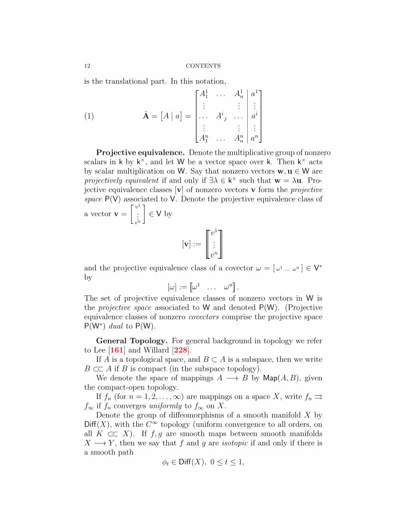
12 CONTENTS
is the translational part. In this notation,
(1) A =[A a
]=
A11 . . . A1
n a1
......
.... . . Ai j . . . ai
......
...An1 . . . Ann an
Projective equivalence. Denote the multiplicative group of nonzeroscalars in k by k×, and let W be a vector space over k. Then k× actsby scalar multiplication on W. Say that nonzero vectors w,u ∈ W areprojectively equivalent if and only if ∃λ ∈ k× such that w = λu. Pro-jective equivalence classes [v] of nonzero vectors v form the projectivespace P(V) associated to V. Denote the projective equivalence class of
a vector v =
[v1
...vn
]∈ V by
[v] :=
v1
...vn
and the projective equivalence class of a covector ω = [ ω1 ... ωn ] ∈ V∗
by[ω] :=
[[ω1 . . . ωn
]].
The set of projective equivalence classes of nonzero vectors in W isthe projective space associated to W and denoted P(W). (Projectiveequivalence classes of nonzero covectors comprise the projective spaceP(W∗) dual to P(W).
General Topology. For general background in topology we referto Lee [161] and Willard [228].
If A is a topological space, and B ⊂ A is a subspace, then we writeB ⊂⊂ A if B is compact (in the subspace topology).
We denote the space of mappings A −→ B by Map(A,B), giventhe compact-open topology.
If fn (for n = 1, 2, . . . ,∞) are mappings on a space X, write fn ⇒f∞ if fn converges uniformly to f∞ on X.
Denote the group of diffeomorphisms of a smooth manifold X byDiff(X), with the C∞ topology (uniform convergence to all orders, onall K ⊂⊂ X). If f, g are smooth maps between smooth manifoldsX −→ Y , then we say that f and g are isotopic if and only if there isa smooth path
φt ∈ Diff(X), 0 ≤ t ≤ 1,

NOTATION AND TERMINOLOGY 13
with φ0 = IX such that g = φ1 f . Denote this relation by f ' g.Suppose (X, d) is a metric space. If x ∈ X, r > 0, define the (open)
ball with center x and radius r as:
Br(x) :=y ∈ X | d(x, y) < r
.
The open balls in a metric space are partially ordered by inclusion.More generally, if A ⊂ X, define
Br(A) :=y ∈ X | ∃a ∈ A such that d(x, a) < r
.
If (X, d) is a metric space, and S, T ⊂⊂ X, then define their Hausdorffdistance
d(S, T ) := infr ∈ R | S ⊂ Br(T ) and T ⊂ Br(S)
.
If X is compact, then the set of closed subsets of X with Hausdorffdistance d is a metric space.
Denote group of isometries of a metric space (X, d) by Isom(X, d),or just Isom(X) if the context is clear.
Fundamental group and covering spaces. If [a, b]γ−−→ X is a
continuous path, write
γ(a)γ γ(b)
to indicate that γ runs between its two endpoints γ(a), γ(b). Fix an
arbitrary basepoint p0 ∈ X. A loop based at p0 is a path p0γ p0. Two
such based loops γ1, γ2 are relatively homotopic if they are homotopicby a homotopy which fixes p0. In that case we write γ1 ' γ2. Inthat The fundamental group π1(M ; p0) corresponding to p0 consists ofrelative homotopy classes [γ] of based loops γ.
The group operation is defined by concatenation of paths: If
[ai, bi]γi−−→ X, for i = 1, 2
are paths, with γ1(b1) = γ2(a2), write γ1 ? γ2 for the continuous path
γ1(a1) γ2(b2),
defined by:
[a1, b2]γ1?γ2−−−−→ X
t 7−→γ1(t) if a1 ≤ t ≤ b1
γ2(t) if a2 ≤ t ≤ b2
If γ1, γ2 are loops based at p0, so is γ1 ? γ2, and concatenation definesan binary operation on π1(X, p0).

14 CONTENTS
The constant path p0 defines an identity element on π1(X, p0) since
p0 ? γ ' γ ? p0 ' γ. Define the inverse of a path [a, b]γ−−→M
[a, b]γ−1
−−−→M
t 7−→ γ(a+ b− t).If γ is a loop based at p0, then
γ ? γ−1 ' γ−1 ? γ ' p0,
obtaining inversion in π1(M ; p0). If [a3, b3]γ3−−→ X with γ2(b2) =
γ3(a2), then
(γ1 ? γ2) ? γ3 ' γ1 ? (γ2 ? γ3),
implying associativity. Thus π1(X, p0) is indeed a group.Under rather general conditions on X (such as being a topological
manifold) defined the universal covering space (corresponding to p0)
X(p0) Π−−→ X
as the collection of relative homotopy classes of paths γ starting at p0,
with the other endpoint at Π(γ). Give X(p0) the coarsest topology suchthat Π is continuous. Then Π is a local homeomorphism, and indeed aGalois covering space with covering group π1(X, p0).
The (left) action on X(p0) by deck transformations from π1(X, p0)
is defined as follows. Choose a point p ∈ X, a path p0η p and a loop
γ based at p0. The action of [γ] on [η] is defined by:
[η][γ]7−−−→ [γ ? η].
The action is free and proper, preserves p = Π([η]). The quotient
map naturally identifies with Π and the quotient space X(p0)/π1(X, p0)naturally identifies with X.
Smooth manifolds. We shall work in the context of smooth man-ifolds, for which a good general reference is Lee [160]. This will enablethe use of differential calculus locally, and notions of smooth mappingsbetween manifolds. A smooth manifold is a Hausdorff space built fromopen subsets of Rn, which we call coordinate patches. The coordinatechanges are general smooth locally invertible maps. If M and N aregiven such structures, a continuous map M −→ N is smooth if in thelocal coordinate charts it is given by a smooth map.
This structure enables the tangent bundle TM , whose points are theinfinitesimal displacements of points in M . That is, to every smooth

NOTATION AND TERMINOLOGY 15
curve (a, b)γ−−→M , and parameter t with a ≤ t ≤ b, is a velocity vector
γ′(t) ∈ Tγ(t)M
representing the infinitesimal effect of displacing γ(t) along γ. Sincethe local coordinates change by general smooth locally invertible maps,there is no natural way of identifying these infinitesimal displacementsat different points. Therefore we attach to each point p ∈M , a “copy”TpM of the model space Rn, which represents the vector space of in-finitesimal displacements of p. It is important to note that althoughthe fibers TpM are disjoint, that the union
TM :=⋃
p∈M
TpM
is topologized as a smooth manifold (indeed, a smooth vector bundle),and not as the disjoint union.
The velocity vector of a smooth curve is a tangent vector at p, whichcan be defined in two equivalent ways:
• Equivalence classes of smooth curves γ(t) with γ(0) = p, wherecurves γ1 ∼ γ2 if and only if
d
dt
∣∣∣∣t=0
f γ1(t) =d
dt
∣∣∣∣t=0
f γ2(t)
for all smooth functions Uf−−→ R, where U ⊂ A is an open
neighborhood of p.
• Linear operators C∞(A)D−−→ R satisfying
(2) D(fg) = D(f)g(p) + f(p)D(g).
The tangent space TpM is a vector space linearizing the smooth man-ifold M at the point p ∈M .
The space of tangent vectors forms a smooth vector bundle TMΠ−−→
M , with fiber Π−1(p) := TpM . If U 3 p is a coordinate patch, thenΠ−1(U) identifies with U × Rn, and this defines a smooth coordinateatlas on TM .
Let M,N be smooth manifolds, and p ∈M . A mapping
Mf−−→ N
is differentiable at p if every infinitesimal displacement v ∈ TpM mapsto an infinitesimal displacement Dpf(v) ∈ TqN , where q = f(p). Thatis, if γ is a smooth curve with γ(0) = p and γ′(0) = v, then we require

16 CONTENTS
that f γ is a smooth curve through q at t = 0; then we call the newvelocity (f γ)′(0) ∈ TqN the value of the differential or derivative
TpM(Df)p−−−−→ TqN
v 7−→ (f γ)′(0)
If P is a third smoooth manifold, and Ng−−→ P is a smooth map, the
composition Mg f−−−−→ P is defined, and is a smooth map. The Chain
Rule expresses the derivative of the composition as the composition of
the derivatives of f and g: and Mf−−→ N
g−−→ P are smooth maps,then the differential of a composition
Mf//
g f
N g
// P
induces a commutative diagram
TxM(Df)x
//
(D(g f)
)x
**Tf(x)N
(Dg)f(x)
// T(gf)(x)P
that is, D(g, f)x = (Dg)f(x) (Df)x.If M,N are smooth manifolds, a diffeomorphism M −→ N is an
invertible smooth mapping whose inverse is also smooth. In particular
a diffeomorphism is a homeomorphism. If Mf−−→ N is a smooth map
and p ∈M such that the differential
TpM(Df)p−−−−→ Tf(p)N
is an isomorphism of vector spaces, the Inverse Function Theorem im-plies the existence of an open neighborhood U 3 p such that the re-striction f |U is a diffeomorphism U → f(U). In particular f(U) ⊂ Nis open and U can be chosen so that (Df)q is an isomorphism for everyq ∈ U . Such a map is called a local diffeomorphism (at p).
Under the C∞ topology, diffeomorphisms M →M form a topologi-cal group, denoted by Diff(M). Indeed Diff(M) has more structure as aFrechet Lie group. IfN is a smooth manifold, then a mapN → Diff(M)is smooth if the natural composition N×M →M is smooth. A smooth
homomorphism R Φ−−→ Diff(M) is called a smooth flow on M .

NOTATION AND TERMINOLOGY 17
Vector fields. A vector field on M is a section of the tangent
bundle TMΠ−−→M , that is a mapping M
ξ−→ TpM such that
Π ξ = IM ,
or equivalently, ξ(p) ∈ TpM . Denote the space of all vector fields onM by Vec(M). Just as individual tangent vectors at p ∈ M definederivations C∞(M) −→ R over the evaluation map
C∞(M) −→ Rf 7−→ f(p)
(as in (2)), vector fields in Vec(M) define derivations of the algebraC∞(M).
Let a < b ∈ R. A smooth curve (a, b)γ−−→ M is an integral curve
for ξ ∈ Vec(M) if and only if
γ′(t) = ξ(γ(t)
)∈ Tγ(t)M
for all a < t < b. If Φ is a smooth flow as above, then for each p ∈M ,
(a, b)Φp−−→M
t 7−→ Φ(t)(p)
is a smooth curve in M with velocity vector field (Φp)′(t) ∈ TΦp(t)M .
In particular
ξ(p) := (Φp)′(0) ∈ TpM (since Φp(0) = p)
defines a smooth vector field ξ ∈ Vec(M).The Fundamental Theorem on Flows is a statement in the converse
direction: every vector field ξ ∈ Vec(M) is tangent to a local flow.That is, through every point there exists a unique maximal integralcurve, defined for some open interval (a, b) containing 0. When M is aclosed manifold), then the integral curves are defined on all of R andcorresponds to a flow Φ on M . Such a vector field is called complete.More generally (Lee [161], Theorem 9.16), if ξ is compactly supported,it is complete.
See Lee [161], §9, for full details; a precise statement of the Funda-mental Theorem on Flows is given in Theorem 9.12. If f is a local dif-feomorphism, and ξ ∈ Vec(N), then define the pullback f ∗ξ ∈ Vec(M)by:
(3) (f ∗ξ)p :=((Df)p
)−1(ξf(p)).
In particular, in the terminology of Lee [161], the vector fields ξ andf ∗ξ are f -related.

18 CONTENTS
Suppose that Mf−−→ N is a smooth map and ξ ∈ V ect(M) and
η ∈ Vec(N) are f -related vector fields, that is,
(Df)p(ξ(p)
)= η(f(p)
), ∀p ∈M.
The Naturality of Flows (Lee [161], Theorem 9.13) implies that if Ψ(t)is the local flow defined by ξ ∈ Vec(M) and Ψ(t) the local flow on Ndefined by η ∈ Vec(N),nthen
f(Φt(p)
)= Ψt
(f(p)
)
whenever these objects are defined.The vector fields onM form a Lie algebra Vec(M) under Lie bracket.

Part 1
Affine and projective geometry


CHAPTER 1
Affine geometry
This section introduces the geometry of affine spaces. After a rig-orous definition of affine spaces and affine maps, we discuss how linearalgebraic constructions define geometric structures on affine spaces.Affine geometry is then transplanted to manifolds. The section con-cludes with a discussion of affine subspaces, vector fields, volume andthe notion of center of gravity.
1.1. Euclidean space
We begin with a short summary of Euclidean geometry in terms ofits underlying space and its group of isometries.
Euclidean geometry can be described in many different ways. Hereis one simple approach. Denote by En the set of points in the vectorspace Rn (that is, ordered n-tuples of real numbers) with the distancefunction
En × End−−→ R
(p, q) 7−→ ‖p− q‖.
Exercise 1.1.1. Let (En, d)g−−→ (En, d) be an isometry. Then
g(p) = Ap+ b
for an orthogonal matrix A ∈ O(n) and a vector b ∈ Rn.
That is, the isometry g of Euclidean n-space En is a composition of thelinear isometry defined by A and the translation
pτb7−−→ p+ b
by b.Two objects X, Y are parallel if they are related by the action of a
translation, in which case we write X ‖ Y .
Exercise 1.1.2. Show that translations form a normal subgroupTrans(En) isomorphic to Rn and
Isom(En) = Trans(En) o O(n).
Deduce that Isom(En) preserves the relation of parallelism.
21

22 1. AFFINE GEOMETRY
Another feature of Euclidean geometry is the notion of angle:
Exercise 1.1.3. Every isometry of En preserves angles. (Hint: usethe fact that angles can be defined in terms of inner products on Rn.)
That is, every isometry is angle-preserving, or conformal. The equiv-alence relation of similarity is generated by the group Sim(En) of con-formal transformations of En.
An element of Sim(En) which is not an isometry is the homothetygiven by scalar multiplication p 7−→ λp, where λ ∈ R and λ 6= ±1.(See §1.5.2 for the general definiton of homotheties.) Denote the groupof scalar multiplications by λ > 0 by R+.
Exercise 1.1.4. The group Sim(En) is generated by Isom(En) andR+. Indeed,
Sim(En) = Sim0(En) n Trans(En)
whereSim0(En) := R+ × O(n)
is the group of linear similarities of En. Explicitly a transformation gof En lies in Sim(En) if it has the form
p 7−→ λA(p) + b
where A ∈ O(n) and λ ∈ R+.
Yet another feature of Euclidean geometry is volume:
Exercise 1.1.5. Show that an orientation-preserving isometry ofEuclidean space is volume-preserving. Show that an orientation-preservingsimilarity transformation preserves volume if and only if it is an isom-etry.
Compare §1.4.2 for further discussion of volume in affine geometry.
1.2. Affine space
What geometric properties of En do not involve the metric notionsof distance, angle and volume? For example, the notion of straight lineis invariant under translations and more general linear maps which arenot Euclidean isometries. Although it admits a metric definition as“the shortest path joining two points,” it enjoys a more fundamentalcharacterization as a curve of zero acceleration, that is, a geodesic.However to define the acceleration of a smooth curve, one needs tocompare the velocity vectors at different points along the curve. Thisis achieved by the parallel transport of the velocity along the curve, andhence involves the notion of parallelism. (This is the notion of an affine

1.2. AFFINE SPACE 23
connection, which is way to “connect” the infinitesimal displacementsat different locations.)
Here is our first definition of an affine transformation:
Definition 1.2.1. An affine transformation of Rn is a mapping ofthe form
Rn g−−→ Rn
p 7−→ Ap+ b
where A ∈ GL(n,R) is an n × n invertible matrix and b ∈ Rn is avector. A is called the linear part of g, and denoted L(g) and b iscalled the translational part of g, and denoted u(g).
Thus an affine transformation g is:
• a translation if and only if L(g) = I;• a Euclidean isometry if and only if L(g) ∈ O(n);• a Euclidean similarity (conformal transformation) if and only
if L(g) ∈ Sim0(Rn) = R+ × O(n);• a volume-preserving affine transformation if and only if L(g) ∈
SL(n,R) .
1.2.1. The geometry of parallelism. Here is a more formal def-inition of an affine space. Although less intuitive, it embodies the ideathat affine geometry is the geometry of parallelism.
Recall that subsets X, Y ⊂ En are parallel (written X ‖ Y ) if andonly if τv(X) = Y for some vector v ∈ Rn. (Here τv ∈ Trans(En)denotes the translation p 7−→ p + v.) Affine geometry is the geom-etry arising from the simply transitive action of the vector space oftranslations (isomorphic to Rn).
Recall that an action of a group G on a space X is simply transi-tive if and only if if for some (and then necessarily every) x ∈ X, theevaluation map
G −→ X
g 7−→ g · xis bijective: that is, for all x, y ∈ X, a unique g ∈ G takes x to y.Equivalently, the action is both:
• Transitive: There is only one orbit, and• Free: No nontrivial element fixes a point.
For further general discussion about group actions, see §A.3.
Definition 1.2.2. Let G be a group. A G-torsor is a space X witha simply transitive G-action.

24 1. AFFINE GEOMETRY
Thus a G-torsor is like the group G, except that the special role ofits identity element is “forgotten.” Thus all the points are regardedas equivalent. What is remembered is the algebraic structure of thetransformations in G which transport uniquely between the points.
Now we give the formal definition of a an affine space:
Definition 1.2.3. An affine space is a V-torsor A, where V is avector space. We call V the vector space underlying A, and denote itby Trans(A), the elements of which are the translations of A.
This abstract approach provides the usual coordinates for an affinespace. Namely, choose a basepoint p0 ∈ A which will correspond tothe origin. That is, it will be labeled by the zero vector 0 ∈ V. Anyother point p ∈ A is related to p0 by a unique translation τ ∈ Trans(A)satisfying p = τ(p0). (This translation exists because the action istransitive, and is unique because the action is free.) Identifying thetransformations Trans(A) with vectors v ∈ V in the usual coordinates,the vector v corresponding to τ is just v = p−p0, and τ is the mapping
Aτ−−→ A
p 7−→ p+ v.
1.2.2. Affine transformations. Here is the second definition ofaffine transformations.
Affine maps are maps between affine spaces which are compatiblewith these simply transitive actions of vector spaces. Suppose A,A′ areaffine spaces with underlying vector spaces
V←→ Trans(A), V′ ←→ Trans(A′).
Then a map
Af−−→ A′
is affine if for each τ ∈ Trans(A), there exists a translation τ ′ ∈Trans(A′) such that the diagram
Af−−−→ A′
τ
yyτ ′
Af−−−→ A′
commutes. Necessarily τ ′ is unique and evidently the correspondence
τL(f)7−−−−→ τ ′
defines a homomorphism of groups V −→ V′, that is, a linear mapbetween vector spaces. This linear map is the linear part of f , denoted

1.2. AFFINE SPACE 25
L(f). Denoting the space of all affine maps A −→ A′ by aff(A,A′) andthe space of all linear maps V −→ V′ by Hom(V,V′), linear part definesa map
aff(A,A′)L−−→ Hom(V,V′)
The set of affine endomorphisms of an affine space A will be denotedby aff(A) and the group of affine automorphisms of A will be denotedAff(A).
The notion of translational part involves choosing basepoints p0 ∈ Aand p′0 ∈ A′, respectively. Then the translational part of f ∈ aff(A,A′)is simply
u(f) := f(p0)− p′0,that is, the vector in V′ corresponding to the translation τf ∈ Trans(A)taking p′0 ∈ A′ to f(p0) ∈ A′. Then (τf )
−1 f maps p0 to p′0 andcorresponds to the linear part L(f) as follows. Let p ∈ A be an arbitrarypoint which corresponds to the vector
x = p− p0 ∈ V,
that is, the translation τ ∈ Trans(A) corresponding to x maps p0 to p,as in §1.2. Then
((τf )
−1 f) τ(p0) = τ ′
((τf )
−1 f)p0 = τ ′(p′0) = p′0 + L(f)x
where τ ′ ∈ Trans(A′) corresponds to L(f)x. Thus f is the compositionof the translation τf ←→ u(f) with the linear part L(f).
The space aff(A,A′) has the natural structure of an affine space.Namely the vector space
Hom(V,V′)⊕ V′.
acts simply transitively on aff(A,A′). Furthermore the Cartesian prod-uct Aff(A) × Aff(A′) acts by composition on aff(A,A′), preserving theaffine structure. (Compare Vey [220] for a discussion of the affinestructure on the space of affine mappings.)
Aff(A) is a Lie group and its Lie algebra identifies with aff(A), whichwe later identify with affine vector fields on A. Furthermore Aff(A) isisomorphic to the semidirect product Aut(V)nV, where V is the normalsubgroup consisting of translations and
Aut(V) = GL(V)
is the group of linear automorphisms of the vector space V←→ Trans(A).Affine geometry is the study of affine spaces and affine maps be-
tween them. If U ⊂ A is an open subset, then a map Uf−−→ A′ is
locally affine if for each connected component Ui of U , there exists anaffine map fi ∈ aff(A,A′) such that the restrictions of f and fi to Ui

26 1. AFFINE GEOMETRY
are identical. Note that two affine maps which agree on a nonemptyopen set are identical.
1.3. The connection on affine space
Now we discuss the structure of an affine space A as a smoothmanifold. To analyze the differentiable structure on A, we considersmooth paths in A and their velociity vector fields, which live in thetangent bundle TA. From this we “connect” the tangent spaces todefine covariant differentiation enabling us to define acceleration asthe covariant derivative of the velocity. Geodesics are curves of zeroacceleration.
1.3.1. The tangent bundle of an affine space. Let γ(t) denotea smooth curve in A; that is, in coordinates
γ(t) =(x1(t), . . . , xn(t)
)
where xj(t) are smooth functions of the time parameter, which rangesin an interval [t0, t1] ⊂ R. The vector γ(t) − γ(t0) corresponds to theunique translation taking γ(t0) to γ(t0), and lies in the vector space Vunderlying A. It represents the displacement of the curve γ as it goesfrom t = t0 to t. Define its velocity vector γ′(t) ∈ V as the derivativeof this path in the vector space V of translations. It represents theinfinitesimal displacement of γ(t) as t varies.
The set of tangent vectors is a vector space, denoted TpM , andnaturally identifies with V as follows. If v ∈ V is a vector, then thepath γ(p,v)(t) defined by:
(4) t 7→ p+ tv = τtv(p)
is a smooth path with γ(0) = p and velocity vector γ′(0) = v. Con-versely, definition above of an infinitesimal displacement, shows thatevery smooth path through p = γ(0) with velocity γ′(0) = v is tangentto the curve (4) as above.
The tangent spaces TpM linearize M as follows. A mapping
Mf−−→M ′
is differentiable at p if every infinitesimal displacement v ∈ TpM mapsto an infinitesimal displacement Dpf(v) ∈ TqM
′, where q = f(p). Thatis, if γ is a smooth curve with γ(0) = q and γ′(0) = v, then we requirethat f γ is a smooth curve through q at t = 0; then we call the new

1.3. THE CONNECTION ON AFFINE SPACE 27
velocity (f γ)′(0) the value of the derivative
TpMDpf−−−→ TqM
′
v 7−→ (f γ)′(0)
1.3.2. Parallel transport. On an affine space A, all the tangentspaces identify with each other. Namely, if x, y ∈ A, let τ ∈ Trans(A)be the unique translation taking x to y. (τ corresponds to the vectory − x.) The differential (Dτ)x maps TxA isomorphically to TyA) andwe denote this by:
TxAPx,y−−−→ TyA
We call this map parallel transport from x to y.
Exercise 1.3.1. Another construction involves the linear structureof V ←→ Trans(A). Namely, the action of V by translations identifies
the vector space V with TxA. Denoting this isomorphism by Vαx−−→
TxA, show that Px,y = αy (αx)−1.
A vector field ξ ∈ Vec(A) is parallel if it is invariant under paralleltransport. That is, Px,y(ξx) = ξy for any x, y ∈ A. This just means
that ξ is a “constant vector field,” defined by a constant map Av−−→ V:
as a differential operator
C∞(A)ξ−→ R
f 7−→ vi(x)∂f
∂xi
where v(x) is constant. Thus V identifies with the space of parallelvector fields on A, and is based by the coordinate vector fields
∂
∂xi∈ Vec(A),
which we abbreviate simply by ∂i.
Exercise 1.3.2. Show that ξ ∈ Vec(A) is parallel if and only if itgenerates a one-parameter group of translations.
Similarly, the dual vector space V∗ identifies with parallel 1-forms asfollows. A 1-form (covector field) on A corresponds to a constant mapA −→ V∗. The basis of parallel covector fields dual to the coordinatebasis ∂1, . . . , ∂n of parallel vector fields is denoted dx1, . . . , dxn (asusual).
Exercise 1.3.3. Show that a parallel 1-form is exact, and henceclosed.

28 1. AFFINE GEOMETRY
1.3.3. Acceleration and geodesics. The velocity vector fieldγ′(t) of a smooth curve γ(t) is an example of a vector field along thecurve γ(t): For each t, the tangent vector γ′(t) ∈ Tγ(t)A. Differenti-ating the velocity vector field raises a significant difficulty: since thevalues of the vector field live in different vector spaces, we need a wayto compare, or to connect them. The natural way is use the simplytransitive action of the group V of translations of A. That is, supposethat γ(t) is a smooth path, and ξ(t) is a vector field along γ(t). Let τ tsdenote the translation taking γ(t+ s) to γ(t), that is, in coordinates:
Aτ ts−−→ A
p 7−→ p+(γ(t+ s)− γ(t)
)
Its differential
Tγ(t+s)ADτ ts−−−→ Tγ(t)A
then maps ξ(t+s) into Tγ(t)A and the covariant derivative Ddtξ(t) is the
derivative of this smooth path in the fixed vector space Tγ(t)A:
D
dtξ(t) :=
d
ds
∣∣∣∣s=0
(Dτ ts)(ξ(t+ s)
)
= lims→0
(Dτ ts)(ξ(t+ s)
)− ξ(t)
s
In this way, define the acceleration as the covariant derivative of thevelocity:
γ′′(t) :=D
dtγ′(t)
A curve with zero acceleration is called a geodesic.
Exercise 1.3.4. Given a point p and a tangent vector v ∈ TpA,show that the unique geodesic γ(t) with
(γ(0), γ′(0)
)= (p,v)
is given by (4).
In other words, geodesics in A are parametrized curves which are Eu-clidean straight lines traveling at constant speed. However, in affinegeometry the speed itself in not defined, but “motion along a straightline at constant speed” is affinely invariant (zero acceleration).
This leads to the following important definition:

1.4. PARALLEL STRUCTURES 29
Definition 1.3.5. Let p ∈ A and v ∈ Tp(A) ∼= V. Then theexponential mapping is defined by:
TpAExpp−−−−→ A
v 7−→ p+ v.
Thus the unique geodesic with initial position and velocity (p,v) equals
t 7−→ Expp(tv) = p+ tv.
1.4. Parallel structures
Many important refinements of affine geometry involve structureswhich are parallel. Parallelism generalizes the notion of “constant”when the targets vary from point to point.
For example, the most familiar geometry is Euclidean geometry,extremely rich with metric notions such as distance, angle, area andvolume. We have seen that affine geometry underlies it with the moreprimitive notion of parallelism. Euclidean geometry arises from affinegeometry by introducing a Riemannian structure on A, which is paral-lel.
Parallel vector fields and 1-forms were introduced back in §1.3.2,where parallel vector fields correspond to vectors in V and parallel 1-forms (parallel covector fields) correspond to covectors in V∗. Now weconsider parallel tensor fields of higher order.
1.4.1. Parallel Riemannian structures. Let B be an inner prod-uct on V and O(V; B) ⊂ GL(A) the corresponding orthogonal group.Then B defines a flat Riemannian metric on A and the inverse image
L−1(O(V; B)) ∼= O(V; B) · Trans(A)
is the full group of isometries, that is, the Euclidean group. If B is a non-degenerate indefinite form, then there is a corresponding flat pseudo-Riemannian metric on A and the inverse image L−1
(O(V; B)
)is the full
group of isometries of this pseudo-Riemannian metric.
Exercise 1.4.1. Show that an affine automorphism g of Euclideann-space Rn is conformal (that is, preserves angles) if and only if its lin-ear part is the composition of an orthogonal transformation and scalarmultiplication.
Such a transformation will be called a similarity transformationand the group of similarity transformations will be denoted Sim(En).The scalar multiple is called the scale factor λ(g) ∈ R+ and defines

30 1. AFFINE GEOMETRY
a homomorphism Sim(En)λ−−→ R+. In general, if g ∈ Sim(En, then
∃A ∈ O(n),b ∈ Rn such that
g(x) = λ(g)Ax+ b.
1.4.2. Parallel tensor fields. Namely, any tangent vector vp ∈TpA extends uniquely to a vector field on A invariant under the groupof translations. As we saw in §1.4.1, Euclidean structures are definedby extending an inner product from a single tangent space to all of E.
Dual to parallel vector fields are parallel 1-forms. Every tangentcovector ωp ∈ T∗pA extends uniquely to a translation-invariant 1-form.
Exercise 1.4.2. Prove that a parallel 1-form is closed. Express aparallel 1-form in local coordinates.
If n = dim(A), then an exterior n-form ω must be f(x) dx1∧· · ·∧dxnin local cooordinates, where f ∈ C∞(A) is a smooth function. Then ωis parallel if and only if f(x) is constant.
Exercise 1.4.3. Prove that an affine transformation g ∈ Aff(A)preserves a parallel volume form if and only if det L(g) = 1.
1.4.3. Complex affine geometry. We have been working en-tirely over R, but it is clear one may study affine geometry over anyfield. If k ⊃ R is a field extension, then every k-vector space is a vectorspace over R and thus every k-affine space is an R-affine space. In thisway we obtain more refined geometric structures on affine spaces byconsidering affine maps whose linear parts are linear over k.
Exercise 1.4.4. Show that 1-dimensional complex affine geometryis the same as (orientation-preserving) 2-dimensional similarity geom-etry.
This structure is another case of a parallel structure on an affinespace, as follows. Recall a complex vector space has an underlyingstructure as a real vector space V. The difference is a notion of scalarmultiplication by
√−1, which is given by a linear map
VJ−−→ V
such that J J = −I. Such an automorphism is called a complexstructure on V, and “turns V into” a complex vector space.
If M is a manifold, an endomorphism field (that is, a (1, 1)-tensorfield) J where, for each p ∈M , the value Jp is a complex structure onthe tangent space TpM is called an almost complex structure. Neces-sarily dim(M) is even.

1.5. AFFINE VECTOR FIELDS 31
Recall that a complex manifold is a manifold with an atlas of co-ordinate charts where coordinate changes are biholomorphic. (Such anatlas is called a holomorphic atlas. Every complex manifold admitsan almost complex structure, but not every almost complex structurearises from a holomorphic atlas, except in dimension two.
Exercise 1.4.5. Prove that a complex affine space is the same asa affine space with a parallel almost complex structure.
1.5. Affine vector fields
A vector field X on A is said to be affine if it generates a one-parameter group of affine transformations. Affine vector fields includeparallel vector fields and radiant vector fields. Parallel vector fields gen-erate one-parameter groups of translations, and radiant vector fieldsgenerate one-parameter groups of homotheties. Covariant differentia-tion provides general criteria characterizing affine vector fields.
1.5.1. Translations and parallel vector fields.
Exercise 1.5.1. A vector field X on A is parallel if, for everyp, q ∈ A, the values Xp ∈ TpA and Xq ∈ TqA are parallel.
Since translation τ by v = q − p is the unique translation taking pto q, this simply means that the differential Dτ maps Xp to Xq.
Exercise 1.5.2. Let X ∈ Vec(A) be a vector field on an affine spaceA. The following conditions are equivalent:
• X is parallel• The coefficients of X (in affine coordinates) are constant.• ∇YX = 0 for all Y ∈ Vec(A).• The covariant differential ∇X = 0.• The linear part L(X) = 0.
The vector space V identifies with the space of parallel vector fields onA. The parallel vector fields form an abelian Lie algebra of vector fieldson A.
1.5.2. Homotheties and radiant vector fields. Another im-portant class of affine vector fields are the radiant vector fields, orinfinitesimal homotheties:
Definition 1.5.3. An affine transformation φ ∈ Aff(A) is a homo-thety if it is conjugate by a translation to scalar mutiplication v 7−→λv, for some scalar λ ∈ R×. An affine vector field is radiant if itgenerates a one-parameter group of homotheties.

32 1. AFFINE GEOMETRY
Observe that a homothety fixes a unique point p ∈ A, which weoften take to be the origin. The only zero of the corresponding radiantvector field is p.
Radiant vector fields are also called Euler vector fields, due to theirrole in Euler’s theorem on homogeneous functions: Recall that a func-
tion Rn f−−→ R is homogeneous of degree m if and only if
f(λx) = λmf(x)
for all λ ∈ R+.
Theorem 1.5.4 (Euler). Suppose that R is the radiant vector fieldvanishing at the origin 0. Then f is homogeneous of degree m if andonly if the directional derivative Rf = mf .
Exercise 1.5.5. Prove Euler’s theorem above.
Radiant vector fields play an important role in our study. Many im-portant examples of affine manifolds admit radiant vector fields, andradiant vector fields provide a link between affine structures in dimen-sion n and projective structures in dimension n− 1.
Exercise 1.5.6. Let R ∈ Vec(A) be a vector field. Then the follow-ing conditions are equivalent:
• R is radiant;• ∇R = IA (where IA ∈ T 1(A; TA) is the identity map TA −→
TA, regarded as an endomorphism field on A);• there exists bi ∈ R for i = 1, . . . , n such that
R =n∑
i=1
(xi − bi) ∂
∂xi.
Note that b = (b1, . . . , bn) is the unique zero of R and that R generatesthe one-parameter group of homotheties fixing b. (Thus a radiant vec-tor field is a special kind of affine vector field.) Furthermore R generatesthe center of the isotropy group of Aff(A) at b, which is conjugate (bytranslation by b) to GL(A). Show that the radiant vector fields on Aform an affine space isomorphic to A.
1.5.3. Affineness criteria. Affine vector fields can be character-ized in terms of the covariant differential operation
T p(M ; TM)∇−−→ T p+1(M ; TM)
where T p(M ; TM) denotes the space of TM -valued covariant p-tensorfields on M , that is, the tensor fields of type (1, p). Thus T 0(M ; TM) =Vec(M), the space of vector fields on M . The space T 1(M ; TM) is

1.5. AFFINE VECTOR FIELDS 33
comprises T∗M -valued vector fields on M , which identify with TM -valued 1-forms, or equivalently endomorphism fields on M .
Exercise 1.5.7. X is affine if and only if it satisfies any of thefollowing equivalent conditions:
• For all Y, Z ∈ Vec(A),
∇Y∇ZX = ∇(∇Y Z)X.
• ∇∇X = 0.• The coefficients of X are affine functions, that is,
X =n∑
i,j=1
(ai jxj + bi)
∂
∂xi
for constants ai j, bi ∈ R.
Write
L(X) =n∑
i,j=1
ai jxj ∂
∂xi
for the linear part (which corresponds to the matrix (ai j) ∈ gl(Rn))and
X(0) =n∑
i=1
bi∂
∂xi
for the translational part (the translational part of an affine vector fieldis a parallel vector field).
Exercise 1.5.8. Under this correspondence, covariant derivativecorresponds to composition of affine maps (matrix multiplication):
∇BA ←→ AB
The Lie bracket of two affine vector fields is given by:
• L([X, Y ]) = [L(X), L(Y )] = L(X)L(Y )− L(X)L(Y )(matrix multiplication)
• [X, Y ](0) = L(X)Y (0)− L(Y )X(0).
In this way the space aff(A) = aff(A,A) of affine endomorphisms A is a Lie algebra.
Let M be an affine manifold. A vector field ξ ∈ Vec(M) is affineif in local coordinates ξ appears as a vector field in aff(A). We denotethe space of affine vector fields on an affine manifold M by aff(M).
Exercise 1.5.9. Let M be an affine manifold.
(1) Show that aff(M) is a subalgebra of the Lie algebra Vec(M).

34 1. AFFINE GEOMETRY
(2) Show that the identity component of the affine automorphismgroup Aut(M) has Lie algebra aff(M).
(3) If ∇ is the flat affine connection corresponding to the affinestructure on M , show that a vector field ξ ∈ Vec(M) is affineif and only if
∇ξυ = [ξ, υ]
∀υ ∈ Vec(M).
1.6. Affine subspaces
Suppose that A1ι→ A is an injective affine map; then we say that
ι(A1) (or with slight abuse, ι itself) is an affine subspace. If A1 isan affine subspace then for each x ∈ A1 there exists a linear subspaceV1 ⊂ Trans(A) such that A1 is the orbit of x under V1 (that is, “anaffine subspace in a vector space is just a coset (or translate) of alinear subspace A1 = x + V1.”) An affine subspace of dimension 0 isthus a point and an affine subspace of dimension 1 is a line.
Exercise 1.6.1. Show that if l, l′ are (affine) lines and
(x, y) ∈ l × l, x 6= y
(x′, y′) ∈ l′ × l′, x′ 6= y′
are pairs of distinct points. Then there is a unique affine map lf−−→ l′
such that
f(x) = x′,
f(y) = y′.
If x, y, z ∈ l (with x 6= y), then define [x, y, z] to be the image of z
under the unique affine map lf−−→ R with f(x) = 0 and f(y) = 1.
Show that if l = R, then [x, y, z] is given by the formula
[x, y, z] =z − xy − x.
This is called an affine parameter along the line.
1.7. Volume in affine geometry
Although an affine automorphism of an affine space A need notpreserve a natural measure on A, Euclidean volume nonetheless doesbehave rather well with respect to affine maps. The Euclidean volumeform ω can almost be characterized affinely by its parallelism: it isinvariant under all translations. Moreover two Trans(A)-invariant vol-ume forms differ by a scalar multiple but there is no natural way to

1.7. VOLUME IN AFFINE GEOMETRY 35
normalize. Such a volume form will be called a parallel volume form.If g ∈ Aff(A), then the distortion of volume is given by
g∗ω = det L(g) · ω.Thus although there is no canonically normalized volume or measurethere is a natural affinely invariant line of measures on an affine space.The subgroup SAff(A) of Aff(A) consisting of volume-preserving affinetransformations is the inverse image L−1(SL(V)), sometimes called thespecial affine group of A. Here SL(V) denotes, as usual, the speciallinear group
Ker(GL(V)
det−−−→ R×)
= g ∈ GL(V) | det(g) = 1.1.7.1. Centers of gravity. Given a finite subset F ⊂ A of an
affine space, its center of gravity or centroid F ∈ A is point associated
with F in an affinely invariant way: that is, given an affine map Aφ−→ A′
we haveφ(F ) = φ(F ).
This operation can be generalized as follows.
Theorem 1.7.1. Let µ be a probability measure on an affine spaceA. Then there exists a unique point x ∈ A (the centroid of µ) such that
for all affine maps Af−→ R,
(5) f(x) =
∫
A
f dµ
Proof. Let (x1, . . . , xn) be an affine coordinate system on A. Letx ∈ A be the points with coordinates (x1, . . . , xn) given by
xi =
∫
A
xi dµ.
This uniquely determines x ∈ A; we must show that (5) is satisfied for
all affine functions. Suppose Af−→ R is an affine function. Then there
exist a1, . . . , an, b such that
f = a1x1 + · · ·+ anx
n + b
and thus
f(x) = a1
∫
A
x1 dµ+ · · ·+ an
∫
A
xn dµ
+ b
∫
A
dµ =
∫
A
f dµ
as claimed.

36 1. AFFINE GEOMETRY
Now let C ⊂ A be a convex body, that is, a convex open subsethaving compact closure. Then C determines a probability measure µCon A by
µC(X) =
∫X∩C ω∫Cω
where ω is any parallel volume form on A.
Proposition 1.7.2. Let C ⊂ A be a convex body. Then the centroidC of C lies in C.
Proof. C is the intersection of halfspaces, that is, C consists ofall x ∈ A such that f(x) > 0 for all affine maps
Af−−→ R
such that f |C > 0. If f is such an affine map, then clearly f(C) > 0.Therefore C ∈ C.
1.7.2. Divergence. If ξ ∈ Vec(M), then the infinitesimal distor-tion of volume is the divergence of ξ, defined as the function div(ξ) suchthat
Lξ(ω) = div(ξ)ω
where ω is (any) parallel volume form and Lξ denotes Lie differentiationwith respect to ξ. If, in coordinates ξ = ξi∂i, then
div(ξ) = ∂iξi
(the usual formula).
Exercise 1.7.3. The Lie algebra of the special affine group SAff(A)consists of affine vector fields of divergence zero.
1.8. Linearizing affine geometry
Associated to every affine space A is an embedding A′ of A as anaffine hyperplane in a vector space W as follows.
Exercise 1.8.1. Let A be an affine space over a field k with un-
derlying vector space V := Trans(A). Let W := V ⊕ k and let Wψ−−→ k
denote linear projection onto the second summand.
• For each s ∈ k, the group V acts simply transitively on theaffine hyperplane ψ−1(s).
– A identifies with ψ−1(1).– V identifies with Ker(ψ) = ψ−1(0).

1.8. LINEARIZING AFFINE GEOMETRY 37
• Define a bijective correspondence betwen n-dimensional affinespaces A and pairs (W, ψ) where W is an n + 1-dimensionalvector space and ψ ∈ W∗ is a nonzero covector, where A cor-responds to ψ−1(1).• Identify the affine group Aff(A) with the subgroup of GL(W)
preserving this hyperplane, as well as the stabilizer of ψ.• If
[A a
]represents an affine transformation with linear part
A and translational part a, show that the corresponding lineartransformation of W is represented by the block matrix[
A a0 1
]
where 0 is the row vector representing the zero map V→ R.
In coordinates, A′(v) =
v1
...vn1
∈ W and ψ = [ 0 ... 0 1 ] ∈ W∗. The
affine transformation has linear part A =
[A1
1 ... A1n
......
An1 ... Ann
]∈ GL(V) and
translational part a =
[a1
...an
]∈ V:
v
[A a
]7−−−−−−→
A1
1 . . . A1n
... Ai j...
An1 . . . Ann
v1
...vj
...vn
+
a1
...ai
...an
=
A1jvi + a1
...Ai jv
j + ai
...Anjv
j + an
A′(v) 7−→
A11 . . . A1
n a1
......
An1 . . . Ann an
. . . . . . . . . . . . . . . . . .0 . . . 0 1
v1
...vn
. .1
=
A1ivi + a1
...Aniv
i + an
. . . . . . . . . .1


CHAPTER 2
Projective geometry
Projective geometry arose historically out of the efforts of Renais-sance artists to understand perspective. Imagine a painter looking at a2-dimensional canvas with one eye closed. His open eye plays the roleof the the origin in the 3-dimensional vector space W and the canvasplays the role of an affine hyperplane A ⊂ W as in §1.8. As the canvastilts, the geometry seen by the painter changes. Parallel lines no longerappear parallel (like the railroad tracks described above) and distanceand angle are distorted. But lines stay lines and the basic relations ofcollinearity and concurrence are unchanged. The change in perspectivegiven by “tilting” the canvas is determined by a linear transformationof W, since a point on A is determined completely by the 1-dimensionallinear subspace of V containing it. (One must solve systems of linearequations to write down the effect of such transformation.) Projec-tive geometry is the study of points, lines and the incidence relationsbetween them.
Projective space closes off affine space — that is, it compactifiesaffine space by adding ideal points at infinity. To develop an intu-itive feel for projective geometry, consider how points in An may go toinfinity:
The easiest way to go to infinity in An is by following geodesics, sincethey have zero acceleration. Furthermore two geodesics approach thesame ideal point if they are parallel. A good model are railroad tracksrunning parallel to each other — they meet ideally at the horizon. Wethus force parallel lines to intersect by attaching ideal points where theextended parallel lines are to intersect.
A good general reference for projective geometry (especially in di-mension two) is Coxeter [64]), as well as Berger [32, 33] and Cox-eter [63]. More classical treatments are Busemann-Kelly [44], Semple-Kneebone [197] and Veblen-Young [216, 217].
2.1. Ideal points
Parallelism of lines in A is an equivalence relation. Define an idealpoint of A as an equivalence class. The ideal set of an affine space A is
39

40 2. PROJECTIVE GEOMETRY
the space P∞(A) of ideal points, with the quotient topology. If l, l′ ⊂ Aare parallel lines, then the point in P∞ corresponding to their paral-lelism class is defined as their intersection. So two lines are parallel ifand only if they intersect at infinity.
Projective space is defined as the union P := A ∪ P∞(A), with asuitable topology. The natural structure on P is perhaps most easilyseen in terms of an alternate, maybe more familiar, description. EmbedA as an affine hyperplane in a vector space W ∼= V⊕k as in §1.8, whereV = Trans(A) is the vector space underlying A. For example, if
p =
p1
...pn
∈ An,
then its embedding in W = kn+1 is the nonzero vector
A′(p) =
p1
...pn
1
∈ W.
Furthermore the line kA′(p) it spans meets the afffine hyperplane A↔kn×1 in a single point. Think of A as the “canvas” or viewing hyper-plane, and the line kA′(p) as the line of sight as the point p is viewedfrom the origin 0 ∈ W (the eye of the painter). The nonzero elementsof this line k×A′(p) form the projective equivalence class [A′(p)].
Now suppose that p travels to infinity along an affine geodesic ` ⊂ A:
p(t) := p+ tv,
where t ∈ k and v ∈ V is a nonzero vector. Denote the correspondingpath of vectors in W by
w(t) := A′(p(t)
)∈ W.
Although limt→∞w(t) does not exist, the corresponding lines k ·w(t)converge to the line k · v corresponding to v ∈ W. This limiting linedefines the ideal point of the affine line `:
limt→∞
[w(t)] = [v]
This motivates the following fundamental definition:
Definition 2.1.1. Let W denote a vector space over k. The projec-tive space associated to W is the space P(W) of projective equivalenceclasses [w] of nonzero vectors w ∈ W, with the quotient topology.

2.2. PROJECTIVE SUBSPACES 41
Thus a point in P(W) (a “projective point”) corresponds to a line (that
is, a one-dimensional linear subspace) in W. If w =
[w1
...wn+1
]∈ W, the
correponding projective point is
p := [w] =
w1
...wn+1
∈ P(W)
and w1, . . . , wn+1 are the homogeneous coordinates of p.Since linear transformations of W preserve lines, GL(W) = Aut(W)
acts on P(W); the induced transformations are the projective transfor-mations or collineations of P(W).
Exercise 2.1.2. The action of GL(W) on P(W) is not effective.Its kernel consists of the group k× of nonzero scalings, which forms thecenter of GL(W). The projective group or collineation group is thequotient
PGL(W) := GL(W)/k×
which does act effectively.
2.2. Projective subspaces
Returning to the projective geometry of the line `, note that theaffine line w(t) in W lies in the linear 2-plane span(p,v) ⊂ W. Theone-dimensional linear subspaces contained in this linear 2-plane is aprojective line.
Definition 2.2.1. Let P = P(W) be a projective space, and let d bea nonnegative integer. A d-dimensional projective subspace S of P isthe collection of all projective equivalence classes [v] of nonzero vectorsv lying in a fixed d + 1-dimensional linear subspace S ⊂ W. We writeS = P(S) and call S the projectivization of S.
Thus a projective line is the projectivization of a linear 2-plane in Wand a projective hyperplane is the projectivization a linear hyperplaneein W.
A linear embedding S1 → S2 ⊂ W of linear subspaces induces anembedding of projective subspaces P(S1) → P(S2) and we say thatthe subspaces P(S1) and P(S2) are incident. Clearly projective trans-formations preserve the relation of incidence. The converse, that anincidence-preserving transformation of projective space, is a deep the-orem, sometimes called the fundaamental theorem of projective geome-try.

42 2. PROJECTIVE GEOMETRY
Exercise 2.2.2. Show that the set of ideal points is a projectivehyperplane.
Suppose that S1, S2 ⊂ P are disjoint projective subspaces. Then,writing Si = P(Si) for respective linear subspaces Si ⊂ W, the projec-tivization P(S1 + S2) is a projective subspace span(S1, S2) ⊂ P and
dim(span(S1, S2)
)= dim(S1) + dim(S2) + 1.
If S1 and S2 are points, then span(S1, S2) is a line, and we use the more
familiar notation←−→S1S2. If Si are projective subspaces and S1 ∩ S2 6= ∅,
then S1 ∩ S2 is a projective subspace and
dim(span(S1, S2)
)+ dim(S1 ∩ S2) = dim(S1) + dim(S2).
Evidently span(S1, S2))
is the smallest projective subspace containingS1 and S2.
2.2.1. Affine patches. Ideal points are only special when projec-tive space is the completion of affine space; by changing the viewinghyperplane, one gets different notions of “ideal.” Indeed, every projec-tive point has neighborhoods which are affine subspaces.
Let P be d-dimensional projective space and H ⊂ P be a projectivehyperplane Then the complement P \H is an affine patch and has thestructure as a d-dimensional affine space with underlying vector spaceV via an affine chart
VA−−→≈
P \H,
defined as follows. Write P = P(W). Choose a covector ψ ∈ W∗ suchthat H = P(V) where V :=
(Ker(ψ). Choose a vector w0 ∈ W with
ψ(w0) = 1 to define an origin in the affine patch. Then
VA(ψ,w0)
−−−−−→ P \Hv 7−→ [w0 + v]
defines an affine chart on P \H. Compare §1.8.Every projective point p ∈ P lies in an affine patch. Writing
p = [X] =
X1
...Xd+1
∈ Pd,
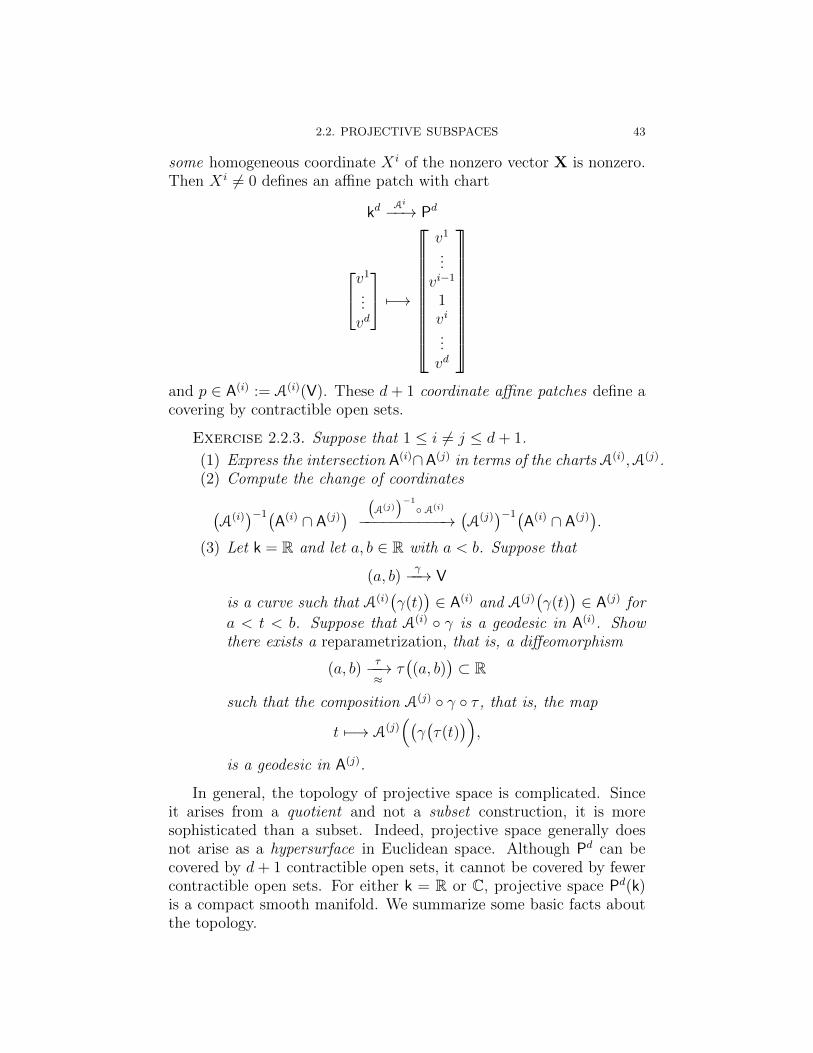
2.2. PROJECTIVE SUBSPACES 43
some homogeneous coordinate X i of the nonzero vector X is nonzero.Then X i 6= 0 defines an affine patch with chart
kdAi−−→ Pd
v1
...vd
7−→
v1
...vi−1
1vi
...vd
and p ∈ A(i) := A(i)(V). These d+ 1 coordinate affine patches define acovering by contractible open sets.
Exercise 2.2.3. Suppose that 1 ≤ i 6= j ≤ d+ 1.
(1) Express the intersection A(i)∩A(j) in terms of the charts A(i),A(j).(2) Compute the change of coordinates
(A(i)
)−1(A(i) ∩ A(j)
)(A(j))−1
A(i)
−−−−−−−−−−→(A(j)
)−1(A(i) ∩ A(j)
).
(3) Let k = R and let a, b ∈ R with a < b. Suppose that
(a, b)γ−−→ V
is a curve such that A(i)(γ(t)
)∈ A(i) and A(j)
(γ(t)
)∈ A(j) for
a < t < b. Suppose that A(i) γ is a geodesic in A(i). Showthere exists a reparametrization, that is, a diffeomorphism
(a, b)τ−−→≈
τ((a, b)
)⊂ R
such that the composition A(j) γ τ , that is, the map
t 7−→ A(j)((γ(τ(t)
)),
is a geodesic in A(j).
In general, the topology of projective space is complicated. Sinceit arises from a quotient and not a subset construction, it is moresophisticated than a subset. Indeed, projective space generally doesnot arise as a hypersurface in Euclidean space. Although Pd can becovered by d+ 1 contractible open sets, it cannot be covered by fewercontractible open sets. For either k = R or C, projective space Pd(k)is a compact smooth manifold. We summarize some basic facts aboutthe topology.

44 2. PROJECTIVE GEOMETRY
Exercise 2.2.4. Suppose k = R. Exhibit Pd(R) as a quotient of theunit sphere Sd ⊂ Rd+1 by the antipodal map. Show that P1(R) ≈ S1
and for d > 1 the fundamental group Pd(R) has order two. Show thatPd(R) is orientable if and only if d is odd.
Exercise 2.2.5. Suppose that k = C. Exhibit Pd(C) as a quotient ofthe unit sphere S2d−1 ⊂ Cd+1 by the group T of unit complex numbers.Show that P1(C) ≈ S2, and Pd(C) is simply connected and orientablefor all d ≥ 1.
Exercise 2.2.6. Find a natural S1-fibration P2d+1(R) −→ Pd(C).
2.3. Projective mappings
Linear mappings Vφ−−→ W between vector spaces define mappings
between the corresponding projective spaces. However, if φ is not in-jective, the corresponding projective map is not defined on all of P(V).We begin discussing with projective maps defined by injectivee linearmaps, particularly emphaszing automorphisms, classically known ascollineations. Collneations arise from liner autmorphisms of the vectorspace W.
2.3.1. Embeddings and Collineations. A projective subspaceS ⊂ P(W) determines a projective map, determined by the linear in-clusion S → W, where S is the linear subspace of W projectivizing toS.
Exercise 2.3.1. Show that an injective projective map P(S −→P(W) is determined by an injeective linear map S −→ W is determinedby an injeective linear map, unique up to composition with a homothetyof S on the left and a homothety of W on the right.
A linear automorphism of a vector spaces W induces an invertible
transformation P(W)φ−−→ P(W). We call such a transformatioon a
collineation or a homography. Evidently a collineation preserves pro-jective subspaces, and the relations between them. An involution is acollineation of order two, that is, φ = φ−1.
Exercise 2.3.2. Let RPn be a real projective space of dimension n,and let φ be an involution of RPn.
• Suppose n is even. Then Fix(φ) is the union of two disjointprojective subspaces of dimensions d1, d2 where d1 +d2 = n−1.• Suppose n = 2m+ 1 is odd. Then either:
– Fix(φ) 6= ∅ and equals the union of two disjoint projectivesubspaces of dimensions d1, d2 where d1 + d2 = n− 1, or

2.3. PROJECTIVE MAPPINGS 45
– Fix(φ) = ∅, and φ leaves invariant an S1-fibration
RPn −→ CPm.
For example, an involution φ of RP2 has an isolated fixed point pand a disjoint fixed line l. In an affine patch containing p, φ looks likea symmetry in p, preserving the local orientation. In contrast, φ lookslike a reflection in l in an affine patch containing l, reversing the localorientation. Since RP2 is nonorientable no global orientation exists toeither preserve or reverse.
Here is an explicit example. The involution defined in homogeneouscoordinates by:
RP2 ι−→ RP2
XYZ
7−→
−X−YZ
fixes the point
p =
001
and the projective line defined by Z = 0, that is, l =[[0 0 1
]]. In
the affine chart A3, the isolated fixed point has coordinates (0, 0) andι appears as the symmetry
[v1
v2
]7−→
[−v1
−v2
].
and in the affine chart A1, the fixed line has coordinates (∗, 0) and ιappears as the reflection
[v1
v2
]7−→
[−v1
v2
]
fixing the vertical axis. That a single reflection can appear simultane-ously as a symmetry in a point and reflection in a line indicates thetopological complexity of P2: A reflection in a line reverses a local ori-entation about a point on the line, and a symmetry in a point preservesa local orientation about the point.
2.3.2. Singular projective mappings. When the linear map φis not injective, then P
(Ker(φ)
)is a projective subspace, upon which
the projectivization [φ] of φ is not defined. For that reason, we call itthe undefined set of [φ], and denote it U([φ]).

46 2. PROJECTIVE GEOMETRY
Exercise 2.3.3. Show that the projective automorphisms of P forma group and that this group (which we denote Aut(P)) has the following
description. If Pf−−→ P is a projective automorphism, then there exists
a linear isomorphism Vf−−→ V inducing f . Indeed there is a short exact
sequence1 −→ R× −→ GL(V) −→ Aut(P) −→ 1
where R× −→ GL(V) is the inclusion of the group of multiplications bynonzero scalars. (Sometimes this quotient
GL(V)/R× ∼= Aut(Pn)
(the projective general linear group) is denoted by PGL(V) or PGL(n+1,R).) Show that if n is even, then
Aut(Pn) ∼= SL(n+ 1;R)
and if n is odd, then Aut(Pn) has two connected components, and itsidentity component is doubly covered by SL(n+ 1;R).
If V,V′ are vector spaces with associated projective spaces P,P′
then a linear map Vf−−→ V′ maps lines through 0 to lines through 0.
But f only induces a map Pf−−→ P′ if it is injective, since f(x) can
only be defined if f( x ) 6= 0 (where x is a point of Π−1(x) ⊂ V−0).Suppose that f is a (not necessarily injective) linear map and let
U(f) = Π(Ker(f)
).
The resulting projective endomorphism of P is defined on the comple-ment P − U(f). If U(f) 6= ∅, the corresponding projective endomor-phism is by definition a singular projective transformation of P. If f issingular, its image is a proper projective subspace, called the range off and denoted R(f).
A projective map P1ι−→ P corresponds to a linear map V1
ι−→V between the corresponding vector spaces (well-defined up to scalarmultiplication). Since ι is defined on all of P1, ι is an injective linearmap and hence corresponds to an embedding. Such an embedding (orits image) will be called a projective subspace. Projective subspaces ofdimension k correspond to linear subspaces of dimension k + 1. (Byconvention the empty set is a projective space of dimension -1.) Notethat the “bad set” U(f) of a singular projective transformation is aprojective subspace. Two projective subspaces of dimensions k, l wherek+l ≥ n intersect in a projective subspace of dimension at least k+l−n.The rank of a projective endomorphism is defined to be the dimensionof its image.

2.3. PROJECTIVE MAPPINGS 47
Exercise 2.3.4. Let P be a projective space of dimension n. Showthat the (possibly singular) projective transformations of P form them-selves a projective space of dimension (n + 1)2 − 1. We denote thisprojective space by End(P). Show that if f ∈ End(P), then
dimN(f) + rank(f) = n− 1.
Show that f ∈ End(P) is nonsingular (in other words, a collineation) ifand only if rank(f) = n, that is, U(f) = ∅. Equivalently, R(f) = P.
An important kind of projective endomorphism is a projection, alsocalled a perspectivity. Let Ak, Bl ⊂ Pn be disjoint projective subspaceswhose dimensions satisfy k+l = n−1. Define the projection Π = ΠAk,Bl
onto Ak from Bl
Pn −Bl Π−−→ Ak
as follows. For every x ∈ Pn − Ak the minimal projective subspace
←→xB := span(x ∪Bl)
containing x∪Bl is unique and has dimension l+ 1. It intersects Ak
transversely in a 0-dimensional projective subspace, that is, a uniquepoint ΠAk,Bl(x), that is:
ΠAk,Bl(x) =←→xB ∩ A.
Perspectivities are projective mappings obtained as restrictions ofprojections:
Exercise 2.3.5. Let A′ ⊂ P be a projective subspace of dimensionk disjoint from B.
• Restriction ΠA,B|A′ is a projective isomorphism A′ → A.• Express an arbitrary projective isomorphism between projective
subspaces as a composition of perspectivities.

48 2. PROJECTIVE GEOMETRY
Figure 2.1. A perspectivity between two lines l, l′ inthe plane. The undefined set of O of the projection isthe center of the perspetivity.
2.3.3. Locally projective maps. If P,P′ are projective spaces
and U ⊂ P is an open set then a map Uf−−→ P′ is locally projective if
for each component Ui ⊂ U there exists a linear map
V(P)fi−−→ V(P′)
such that the restrictions of f Π and Π fi to Π−1Ui agree. Locallyprojective maps (and hence also locally affine maps) satisfy the UniqueExtension Property: if U ⊂ U ′ ⊂ P are open subsets of a projectivespace with U nonempty and U ′ connected, then any two locally pro-jective maps f1, f2 : U ′ −→ P′ which agree on U must be identical.(Compare §5.1.1.)
The passage between the geometry of P and the algebra of V is a“dictionary” between linear algebra and projective geometry. Linearmaps and linear subspaces correspond geometrically to projective mapsand projective subspaces: inclusions, intersections and linear spans cor-respond to incidence relations in projective geometry. Thus projectivegeometry lets us visually understand linear algebra and linear algebraenables to prove theorems in geometry by calculation.
Exercise 2.3.6. Let U ⊂ P be a connected open subset of a pro-
jective space of dimension greater than 1. Let Uf−→ P be a local dif-
feomorphism. Then f is locally projective if and only if for each linel ⊂ P, the image f(l ∩ U) is a line.

2.4. AFFINE PATCHES 49
2.4. Affine patches
Let H ⊂ P be a projective hyperplane (projective subspace of codi-mension one). Then the complement P−H has a natural affine geom-etry, that is, is an affine space in a natural way. Indeed the group ofprojective automorphisms P→ P leaving fixed each x ∈ H and whosedifferential TxP→ TxP is a volume-preserving linear automorphism isa vector group acting simply transitively on A = P \H. Moreover thesubgroup of Aut(P) leaving H invariant is Aff(A). In this way affinegeometry embeds in projective geometry.
Here is how it looks in terms of matrices. Let A = Rn; then theaffine subspace of
V = Trans(A)⊕ R = Rn+1
corresponding to A is Rn × 1 ⊂ Rn+1, the point of A with affine orinhomogeneous coordinates (x1, . . . , xn) has homogeneous coordinates[x1, . . . , xn, 1]. Let f ∈ Aff(E) be the affine transformation with linearpart A ∈ GL(n;R) and translational part b ∈ Rn, that is, f(x) =Ax+ b, is then represented by the (n+ 1)-square matrix
[A b0 1
]
where b is a column vector and 0 denotes the 1× n zero row vector.
2.4.1. Projective vector fields. In the affine space An, let
B(An) −→ An
denote the bundle of bases, more commonly known as the affine framebundle over An: its fiber Bp over a point p ∈ An consists of the set ofbases for the tangent space TpA
n. Using the simply transitive action ofkn = Trans(An) on An, the total space B(An) is a torsor for the affineautomorphism group Aff(An): an affine automorphism is determineduniquely by its action on a basepoint p0 ∈ An and a basis β0 ∈ Bp0 ofTpA
n. and every (p, β) ∈ B is the image of (p0, β).Let g ∈ Aut(Pn be a projective automorphism. Fixing a basepoint
p0 and a basis β0 of Tp0An, let h ∈ Aff(An) be the unique affine auto-morphism taking (p0, β0) to (p, β). Then h−1 g is a projective auto-morphism fixing p0 and acts identically on Tp0Pn = Tp0An. In the affinechart An+1 where p0 is the origin, such a projective transformation is

50 2. PROJECTIVE GEOMETRY
defined in homogeneous coordinates by:
X1
...Xn
Xn+1
7−→
X1
...Xn
∑ni=1 ξiX
i +Xn+1
for a row vector ξ† for ξ ∈ kn, that is, by the block matrix[In 0ξ 1
].
In affine coordinates such a transformation is given by
(x1, . . . , xn)gξ7−−→
( x1
1 +∑n
i=1 ξixi, . . . ,
xn
1 +∑n
i=1 ξixi
).
Exercise 2.4.1. Show that this group is isomorphic to a n-dimensionalvector group, and gξ lies in the one-parameter group
t 7−→ gtξ.
The corresponding vector field equals the product
−n∑
i=1
ξixiR
where R is the radiant vector field defined in §1.5.2. Denote the Liealgebra of such vector fields by g1, the Lie algebra of parallel vectorfields on An by g−1, and the Lie algebra of linear vector fields on An
by g0, show that, for λ = 0,±1, the subalgebra gλ of the Lie algebra gof projective vector fields equals the λ-eigenspace of AdR. Furthermore[gλ, gµ] ⊂ gλ+µ where gν := 0 if ν 6= 0,±1. In particular as a vectorspace g decomposes as a direct sum
g = g−1 ⊕ g0 ⊕ g1∼= kn ⊕ gl(n)⊕ kn.
Describe the corresponding group-theoretic decomposition of the projec-tive automorphiism group
Aut(Pn) := PGL(n+ 1).
2.5. Classical projective geometry
2.5.1. One-dimensional reflections. Let l be a projective linex, z ∈ l be distinct points. Then there exists a unique reflection (aharmonic homology in classical terminology)
lρx,z−−−→ l

2.5. CLASSICAL PROJECTIVE GEOMETRY 51
a
Figure 2.2. The four points on the horizontal line forma harmonic quadruple. Such a quadruple is characterizedby having cross-ratio −1.
whose fixed-point set equals x, z. We say that a pair of points y, ware harmonic with respect to x, z if ρx,z interchanges them. In that caseone can show that x, z are harmonic with respect to y, w. Furthermorethis relation is equivalent to the existence of lines p, q through x andlines r, s through z such that
y =←−−−−−−−−−→(p ∩ r)(q ∩ s) ∩ l(6)
z =←−−−−−−−−−→(p ∩ s)(q ∩ r) ∩ l(7)
This leads to a projective-geometry construction of reflection, asfollows. Let x, y, z ∈ l be fixed; we seek the harmonic conjugate of ywith respect to x, z, that is, the image Rx,z(y). Erect arbitrary lines(in general position) p, q through x and a line r through z. Through ydraw the line
l′ :=←−−−−−−→y (r ∩ q)
through r ∩ q; join its intersection with p with z to form a line:
s =←−−−−−−→z (p ∩ l′) .
Then Rx,z(y) will be the intersection of s with l.

52 2. PROJECTIVE GEOMETRY
Figure 2.3. Non-Euclidean tesselations by equilateraltriangles

2.5. CLASSICAL PROJECTIVE GEOMETRY 53
Exercise 2.5.1. Consider the projective line P1 = R∪ ∞. Showthat for every rational number x ∈ Q there exists a sequence
x0, x1, x2, x3, . . . , xn ∈ P1
such that:
• x = limi→∞ xi;• x0, x1, x2 = 0, 1,∞;• For each i ≥ 3, there is a harmonic quadruple (xi, yi, zi, wi)
withyi, zi, wi ∈ x0, x1, . . . , xi−1.
If x is written in reduced form p/q then what is the smallest n for whichx can be reached in this way?
Exercise 2.5.2 (Synthetic arithmetic). Using the above syntheticgeometry construction of harmonic quadruples, show how to add, sub-tract, multiply, and divide real numbers by a straightedge-and-pencilconstruction. In other words, draw a line l on a piece of paper andchoose three points to have coordinates 0, 1,∞ on it. Choose arbitrarypoints corresponding to real numbers x, y. Using only a straightedge(not a ruler!) construct the points corresponding to
x+ y, x− y, xy, and x/y if y 6= 0.
2.5.2. Fundamental theorem of projective geometry. Oneversion of what is sometimes called the fundamental theorem of projec-tive geometry is that the projective transformations (defined by lineartransformations of the associated vector space) are precisely the trans-formations of projective space which preserve the ternary relation ofcollinearity (hence collineations). Collinearity is a special instance ofthe set of incidence relations between projective subspaces. For exam-ple, two distinct projective points p, q are incident to a unique projec-tive line←→p, q and (p, q, r) is a collinear triple if and only if r ∈ ←→p, q. We donot develop this theory in detail, but refer to the texts of Berger [34, 33]and Coxeter [63] for discussion, and in particular the relation with au-tomorphisms of the ground field k.
If l ⊂ P and l′ ⊂ P′ are projective lines, part of the FundamentalTheorem of Projective Geometry asserts that for given triples x, y, z ∈ land x′, y′, z′ ∈ l′ of distinct points there exists a unique projective map
lf−−→ l′
x 7−→ x′
y 7−→ y′
z 7−→ z′

54 2. PROJECTIVE GEOMETRY
If w ∈ l then the cross-ratio [w, x, y, z] is defined to be the image of w
under the unique collineation lf−−→ P1 with
xf7−−→ 1
yf7−−→ 0
zf7−−→ ∞
If l = P1, then this linear fractional transformation is: 1
f(w) :=w − yw − z
/x− yx− z
so
(8) [w, x, y, z] :=w − yw − z
/x− yx− z
Cross-ratio extends to quadruples of four points, of which at least threeare distinct.
Exercise 2.5.3. Let σ be a permutation on four symbols. Showthat there exists a linear fractional transformation Φσ such that
[xσ(1), xσ(2), xσ(3), xσ(4)] = Φσ([x1, x2, x3, x4].
In particular determine which permutations leave the cross-ratio invari-ant.
The cross-ratio is a function of 4 variables, and therefore transformsunder the action of the symmetric group S4 on 4 symbols. The groupS4 is a split extension
Z/2⊕ Z/2ES4 S3
where the normal subgroup Z/2⊕ Z/2 consists of products of disjointtranspositions and a section S3 → S4 corresponds to the inclusion2, 3, 4 → 1, 2, 3, 4.
Exercise 2.5.4. Show that the cross-ratio is invariant under thenormal subgroup Z/2 ⊕ Z/2, and transforms under S3 = Aut2, 3, 4
1The literature has several variations of the cross-ratio; the version here isused by Veblen-Young [216],Kneebone-Semple[197], Coxeter [65], Ahlfors [2].Other versions can be found in Goldman [96], Hubbard [121], Ovsienko-Tabachnikov [183]. and Kaufman [].

2.5. CLASSICAL PROJECTIVE GEOMETRY 55
by the rules, where z = [z1, z2, z3, z4]:
[z1, z2, z4, z3] = 1/z
[z1, z3, z2, z4] = 1− z[z1, z3, z4, z2] = 1− 1/z
[z1, z4, z2, z3] = 1/(1− z)
[z1, z4, z3, z2] = z/(z − 1)
This corresponds to an embedding S3 → GL(2,Z) taking
(34) 7−→[0 11 0
]
(23) 7−→[−1 10 1
]
(234) 7−→[1 −11 0
]
(243) 7−→[
0 1−1 1
]
(24) 7−→[−1 0−1 +1
]
which induces an isomorphism S3∼= GL(2,Z/2).
A pair w, x is harmonic with respect to the pair y, z (in whichcase we say that (x, y, w, z) is a harmonic quadruple) if and only if thecross-ratio [x, y, w, z] = −1.
Exercise 2.5.5. When z = ∞, the expression for the cross-ratiosimplifies:
[x, y, w,∞] :=x− wy − w
and defines a fundamental affine invariant.
• (x, y, z,∞) is a harmonic quadruple if and only if y is themidpoint of xz.• Suppose (x, y, w), (x′, y′, w′) are ordered triples of distinct points
of A1. Show that [x, y, w,∞] = [x′, y′, w′,∞] if and only if ∃g ∈Aff(A1) such that
x′ = g(x)
y′ = g(y)
w′ = g(w).

56 2. PROJECTIVE GEOMETRY
The process of extending a triple of points on P1 to a harmonicquadruple is equivalent to applying a projective reflection in one pairto the remaining element. This process is called harmonic subdivision.Iterated harmonic subdivisions produce a countable dense subsets ofP1 corrresponding to the rational numbers Q ⊂ R. Such a subset iscalled a harmonic net (Coxeter [64], §3.5) or a net of rationality inVeblen-Young [216],p.84). Compare also Busemann-Kelly [44], §I.6.These ideas provide an approach to the fundamental theorem:
Exercise 2.5.6. Let P1 f−→ P1 be a homeomorphism. Show that thefollowing conditions are equivalent:
• f is projective;• f preserves harmonic quadruples• f preserves cross-ratios, that is, for all quadruples (x, y, w, z),
the cross-ratios satisfy
[f(x), f(y), f(w), f(z)] = [x, y, w, z].
Determine the weakest hypothesis on f to obtain these conditions.
2.5.3. Distance via cross-ratios. For later use in §12.1, here aresome explicit formulas for cross-ratios on 1-dimensional spaces R+ andI. Their infinitesimal forms yield the Poincare metrics on R+ and I.
Exercise 2.5.7. (Parameters on the positive ray and unit intervals)
[0, ea, eb,∞] = [−1, tanh(a/2), tanh(b/2), 1] = eb−a
2.5.4. Products of reflections. If φ, ψ are collineations, each ofwhich fix a point O ∈ P, their composition φψ = φ ψ fixes O. Inparticular its derivative
D(φψ)O = (DφO) (DψO)
acts linearly on the tangent space TOP. We consider the case when φ, ψare reflections in P2. As in Exercise 2.3.2, a reflection φ is completelydetermined by its set Fix(φ) which consists of a point pφ and a line lφsuch that pφ /∈ lφ. Define
O := lφ ∩ lψand PO the projective line whose points are the lines incident to O.
Exercise 2.5.8. Let ρ denote the cross-ratio of the four lines
l,←→Op,
←→Op′, l′
as elements of PO.

2.6. ASYMPTOTICS 57
• The linear automorphism
TOPD(φψ)O−−−−−→ TOP
of the tangent space TOP leaves invariant a postive definiteinner product gO on TOP.• Furthermore D(φψ)O represents a rotation of angle θ in the
tangent space TO(P) with respect to gO if and only if
ρ =1
2(1 + cos θ)
for 0 < θ < π and is a rotation of angle π (that is, an involu-tion) if and only if p ∈ l′ and p′ ∈ l.
2.6. Asymptotics of projective transformations
We shall be interested in the singular projective transformationssince they occur as limits of nonsingular projective transformations.The collineation group Aut(P) of P = Pn is a large noncompact groupwhich is naturally embedded in the projective space End(P) as an opendense subset as in Exercise 2.3.4. Thus understanding precisely whatit means for a sequence of collineations to converge to a (possibly sin-gular) projective transformation is crucial.
A singular projective transformation of P is a projective map fdefined on the complement of a projective subspace U(f) ⊂ P, calledthe undefined subspace of f and taking values in a projective subspaceR(f) ⊂ P, called the range of f . Furthermore
dim P = dim U(f) + dim R(f) + 1.
Proposition 2.6.1. Let gm ∈ Aut(P) be a sequence of collineationsof P and let g∞ ∈ End(P). Then the sequence gm converges to g∞ inEnd(P) if and only if the restrictions gm|K converge uniformly to g∞|Kfor all compact sets K ⊂⊂ P− U(g∞).
Convergence in End(P) may be described as follows. Let P = P(V)where V ∼= Rn+1 is a vector space. Then End(P) is the projective spaceassociated to the vector space End(V) of (n + 1)-square matrices. Ifa = (aij) ∈ End(V) is such a matrix, let
‖a‖ =√
Tr(aa†) =
√√√√n+1∑
i,j=1
|aij|2
denote its Euclidean norm; projective endomorphisms then correspondto matrices a with ‖a‖ = 1, uniquely determined up to the antipodal

58 2. PROJECTIVE GEOMETRY
map a 7→ −a. The following lemma will be useful in the proof ofProposition 2.6.1.
Lemma 2.6.2. Let V,V′ be vector spaces and let Vfn−→ V′ be a se-
quence of linear maps converging to Vf∞−→ V′. Let K ⊂ V be a compact
subset of V − Ker(f∞). Define:
Vfi−−→ V′
x 7−→ fi(x)
‖fi(x)‖.
Then fn converges uniformly to f∞ on K as n −→∞.
Proof. Choose C > 0 such that C ≤ ‖f∞(x)‖ ≤ C−1 for x ∈ K.
For ε > 0, ∃N such that if n > N , then ∀x ∈ K,
‖f∞(x)− fn(x)‖ < Cε
2,
∣∣∣∣1−fn(x)
‖f∞(x)‖
∣∣∣∣ <ε
2.(9)
Let x ∈ K. Then∥∥∥∥fn(x)− f∞(x)
∥∥ =
∥∥∥∥fn(x)
‖fn(x)‖− f∞(x)
‖f∞(x)‖
∥∥∥∥
=1
‖f∞(x)‖
∥∥∥∥‖f∞(x)‖‖fn(x)‖
fn(x)− f∞(x)
∥∥∥∥
≤ 1
‖f∞(x)‖
( ∥∥∥∥‖f∞(x)‖‖fn(x)‖
fn(x)− fn(x)
∥∥∥∥
+ ‖fn(x)− f∞(x)‖)
=
∣∣∣∣1−‖fn(x)‖‖f∞(x)‖
∣∣∣∣ +1
‖f∞(x)‖‖fn(x)− f∞(x)‖
<ε
2+ C−1(
Cε
2) = ε
(by (9)
),
completing the proof of Lemma 2.6.2.
Proof of Proposition 2.6.1. Suppose gm is a sequence of lo-cally projective maps defined on a connected domain Ω ⊂ P converging

2.6. ASYMPTOTICS 59
uniformly on all compact subsets of Ω to a map
Ωg∞−−−→ P′.
Lift g∞ to a linear transformation g∞ of norm 1, and lift gm to lineartransformations gm, also linear transformations of norm 1, convergingto g∞. Then
gm −→ g∞in End(P). Conversely if gm −→ g∞ in End(P) and
K ⊂ P− U(g∞),
choose lifts as above and K ⊂⊂ V such that Π(K) = K. By Lemma 2.6.2,
gm/‖gm‖ ⇒ g∞/‖g∞‖on K. Hence gm|K ⇒ g∞|K , completing the proof of Proposition 2.6.1.
2.6.1. Some examples. Let us consider a few examples of thisconvergence. Consider the case first when n = 1. Let λm ∈ R be a se-quence converging to +∞ and consider the projective transformationsgiven by the diagonal matrices
gm =
[λm 00 (λm)−1
]
Then gm −→ g∞ where g∞ is the singular projective transformationcorresponding to the matrix
g∞ =
[1 00 0
]
— this singular projective transformation is undefined at U(g∞) =[0, 1]; every point other than [0, 1] is sent to [1, 0]. It is easy to seethat a singular projective transformation of P1 is determined by theordered pair of points
(U(f),R(f)
). Note that in the next example,
the two points U(φ∞),R(φ∞))
coincide.
Exercise 2.6.3. Consider the sequence of projective transforma-tions of P1
φn(x) :=x
1− nx, as n −→ +∞• Show that the pointwise limit equals the constant function 0:
limn→∞
φn(x) = 0, ∀x ∈ P1.
• Show that φn does not converge uniformly on any subset S ⊂P1 which contains an infinite subsequence sj > 0 with sj 0as j −→∞.

60 2. PROJECTIVE GEOMETRY
• Show that φn does converge to the singular projective trans-formation φ∞ defined on the complement of U(φ∞) = 0 andhas constant value 0.• Use this idea, together with the techniques involved in the proof
of Lemma 2.6.2, to prove a statement converse to Proposi-tion 2.6.1: If gn ∈ Aut(P) is a sequence of projective trans-formations converging to a singular projective transformationg∞ ∈ End(P), then, for any open subset S ⊂ P which meetsU(g∞), the restrictions gn|S do not converge uniformly.
Exercise 2.6.4. (1) The projective group PGL(2,R) = Aut(RP1)is an open dense subset of End(RP1) ≈ RP3. Its complementnaturally identifies with the Cartesian product RP1 ×RP1 un-der the correspondence
End(RP1) \ Aut(RP1)←→ RP1 × RP1
[f ]←→(U(f),R(f)
)
(2) Prove the analogous statements for PGL(2,C) and CP1, thatis, when R is replaced by C.
(3) Show that if Γ < PGL(2,C) is a discrete subgroup with limitset Λ ⊂ CP1, then Γ \ Γ identifies with Λ× Λ ⊂ CP1 × CP1.
2.6.2. Higher dimensional projective maps. More interestingphenomena arise when n = 2. Let gm ∈ Aut(P2) be a sequence ofdiagonal matrices
λm 0 00 µm 00 0 νm
where 0 < λm < µm < νm and λmµmνm = 1. Corresponding to thethree eigenvectors (the coordinate axes in R3) are three fixed points
p1 = [1, 0, 0], p2 = [0, 1, 0], p3 = [0, 0, 1].
They span three invariant lines
l1 =←−−→p2 p3 , l2 =←−−→p3 p1 , l3 =←−−→p3 p1 .
Since 0 < λm < µm < νm, the collineation has an repelling fixed pointat p1, a saddle point at p2 and an attracting fixed point at p3. Pointson l2 near p1 are repelled from p1 faster than points on l3 and pointson l2 near p3 are attracted to p3 more strongly than points on l1. Sup-pose that gm does not converge to a nonsingular matrix; it follows thatνm −→ +∞ and λm −→ 0 as m −→ ∞. Suppose that µm/νm −→ ρ;

2.6. ASYMPTOTICS 61
then gm converges to the singular projective transformation g∞ deter-mined by the matrix
0 0 00 ρ 00 0 1
which, if ρ > 0, has undefined set U(g∞) = p1 and range l1; otherwiseU(g∞) = l2 and Image(g∞) = p2.
2.6.3. Limits of similarity transformations. Convergence tosingular projective transformations is perhaps easiest for translationsof affine space, or, more generally, Euclidean isometries.
Exercise 2.6.5. Suppose gm ∈ Isom(En) be a divergent sequenceof Eucidean isometries. Show that ∃p ∈ Pn−1
∞ a subsequence gmk , thatgmk |K ⇒ p for every compact K ⊂⊂ En.
Indeed the boundary of the translation group V of An is the projectivespace Pn−1
∞ . More generally the boundary of Isom(En) identifies withPn−1∞ .
Exercise 2.6.6. Suppose gm ∈ Sim(En) be a divergent sequence ofsimilarities of Eucidean space. Then ∃ a subsequence gmk , and a point
p ∈ En∐
Pn−1∞
such that one of the three possibilities occur:
• p ∈ Pn−1∞ and gmk |K ⇒ p, ∀K ⊂⊂ En;
• p ∈ Pn−1∞ and ∃q ∈ En such that
gmk |K ⇒ p, ∀K ⊂⊂ En \ q;
• p ∈ En∞ and
gmk |K ⇒ p, ∀K ⊂⊂ En.
The scale factor homomorphism Sim(En)λ−−→ R+ defined in §1.4.1 of
Chapter 1 controls the asymptotics of linear similarities. The two lat-ter cases occur when limk→∞ λ(gmk) = ∞ and limk→∞ λ(gmk) = 0,respectively.
These results will be used in Fried’s classification of closed similaritymanifolds (§11.4 of Chapter 11).

62 2. PROJECTIVE GEOMETRY
2.6.4. Normality domains. Convergence to singular projectivetransformations closely relate to the notion of normality, due to Kulkarni-Pinkall [156]. Let G be a group acting on a space X strongly effectively.A point x ∈ X is a point of normality with respect to G if and only ifx admits an open neighborhood W such the the set of restrictions
G|W := g|W | g ∈ Gis a compact subset of Map(W,X) with respect to the compact-opentopology on Map(W,X). (This means that G|W is a normal familyin the sense of Montel.) Denote the set of points of normality byNor(G,X). Clearly Nor(G,X) is a G-invariant open subset of X, calledthe normality domain.
Proposition 2.6.7. Let Γ < Aut(P) be a discrete group of collineationsof a projective space P. Let Γ ⊂ End(P) denote its closure in theset of singular projective transformations. Then the normality domainNor(Γ, X) consists of the complement
UΓ := X \⋃
γ∈Γ
U(γ)
in P of the union⋃γ∈Γ U(γ).
Proof. Observe first that⋃γ∈Γ U(γ) ⊂⊂ X since each projective
subspace U(γ) ⊂⊂ X. Since the parameter space Γ is compact. Thusit’s closed, and its complement
UΓ := X \⋃
γ∈Γ
U(γ)
is open. We claim that UΓ = Nor(Γ, X).We first show any point x ∈ UΓ is a point of normality. To this end,
we show that. set of restrictions Γ|UΓis precompact in Map(UΓ, X).
This follows immediately from Proposition 2.6.1 as follows. Consideran infinite sequence γn ∈ Γ. Proposition 2.6.1 ensures a subsequenceγn and a singular projective transformation γ∞ ∈ End(P), such that
γn|K ⇒ γ∞|K , ∀K ⊂⊂ UΓ
as desired. (Since K ∩ U(γ∞) = ∅, the restriction γ∞|K is defined.)Conversely suppose that x ∈ U(γ) for some γ ∈ Γ. Choose a se-
quence gn ∈ Γ converging to γ, and a precompact open neighborhoodS 3 x. By Exercise 2.6.3, the restrictions gn|S do not converge uni-formly, and the restrictions to the closure S ⊂ X do not convergeuniformly. Thus x /∈ Nor(Γ, X) as claimed.

CHAPTER 3
Duality and non-Euclidean geometry
The axiomatic development of projective geometry enjoys a basicsymmetry: In P2, a pair of distinct points lie on a unique line and a pairof distinct lines meet in a unique point. Consequently any statementabout the geometry of P2 can be dualized by replacing “point” by“line,” “line”by “point,” “collinear” with “concurrent,” etc, as long asit is done in a completely consistent fashion.
One of the oldest nontrivial theorems of projective geometry is Pap-pus’ theorem (300 A.D.), asserting that if l, l′ ⊂ P2 are distinct linesand A,B,C ∈ l and A′, B′, C ′ ∈ l′ are triples of distinct points, thenthe three points
←→AB′ ∩
←→A′B,
←−→BC ′ ∩
←−→B′C,
←→CA′ ∩
←→C ′A
are collinear. Dual to Pappus’ theorem is the following: if p, p′ ∈ P2 aredistinct points and a, b, c are distinct lines all passing through p anda′, b′, c′ are distinct lines all passing through p′, then the three lines
←−−−−−−−−−−→(a ∩ b′) (a′ ∩ b),
←−−−−−−−−−−→(b ∩ c′) (b′ ∩ c),
←−−−−−−−−−−→(c ∩ a′) (c′ ∩ a)
are concurrent. (According to [63], Hilbert observed that Pappus’ the-orem is equivalent to the commutative law of multiplication.)
This chapter introduces the projective models for elliptic and hy-perbolic geometry through the classical notion of polarities. We beginby working over both R and C, but specialize to the case k = R whenwe discuss important cases of polarities:
• Elliptic polarities, corresponding to definite symmetric bilinearforms, and leading to elliptic (spherical) geometry;• Hyperbolic polarities, corresponding to Lorentzian bilinear
forms, and leading to hyperbolic geometry;• Null polarities, corresponding to nondegeneraate skew-symmetric
bilinear forms, and leading to contact projective geometry (inodd dimensions). (Compare Semple and Kneebone [197].)
See Ratcliffe [189] for a good elementary treatment of the Beltrami-Klein model for hyperbolic geometry, as well as Thurston [212], §2.3.
63

64 3. DUALITY AND NON-EUCLIDEAN GEOMETRY
The various derivations of hyperbolic geometry are aided by symme-try. The Beltrami-Klein metric generalizes to the Hilbert metric onconvex domains. For an extensive modern discussion of Hilbert geome-try, see Papadopoulos-Troyanov [185]. These, in turn, are special casesof intrinsic metrics, which we introduce here, and discuss later in thecontext of affine and projective structures on manifolds.
3.1. Dual projective spaces
In terms of our projective geometry/linear algebra dictionary, pro-jective duality translates into duality between vector spaces as follows.Let P = P(W) be a projective space associated to the vector space W.A nonzero linear functional
Wψ−−→ k
defines a projective hyperplane Hψ in P; two such functionals definethe same hyperplane if and only if they are projectively equivalent,that is, they differ by scalar multiplication by a nonzero scale factor.Equivalently, they determine the same line in the vector space W∗ dualto W.
The projective space P∗ dual to P consists of lines in the dual vectorspace W∗, which correspond to hyperplanes in P. The line joiningtwo points in P∗ corresponds to the intersection of the correspondinghyperplanes in P, and a hyperplane in P∗ corresponds to a point in P.
Exercise 3.1.1. Show that an n-dimensional projective space en-joys a natural correspondence
k − dimensional subspaces of P ←→l − dimensional subspaces of P∗
where k + l = n− 1.
Since vector spaces of the same dimension are isomorphic, a projec-tive space P is projectively isomorphic to the dual of P∗, but in manydifferent ways.
Let Pf−−→ P′ be a projective map. Then for each hyperplane H ′ ⊂
P′ the preimage f−1(H ′) is a hyperplane in P. This defines a projective
map (P′)∗f∗−−→ P∗.
Here is the detailed construction. Suppose that f is defined by a
linear mapping of vector spaces WF−−→ W′, where P,P′ projectivize
W,W′ respectively. Since f is defined on all of P, the linear map F

3.2. CORRELATIONS AND POLARITIES 65
is injective. The projective hyperplane H corresponds to the linearhyperplane
S := Ker(ψ) ⊂ W,
for some nonzero covector ψ ∈ W∗. Since F−1(S) = Ker(ψ F ), thepreimage f−1(H ′) is the projective hyperplane defined by the covectorψ F ∈ (W′)∗.
Exercise 3.1.2. If f is the projectivization of a linear map WF−−→
W′, show that f ∗ is the projectivization of the dual map (W′)∗F ∗−−−→
W∗ given by matrix transpose. That is, represent F by a matrix Mby choosing bases of W and W′ respectively. Show that the matrixrepresenting F ∗ in the respective dual bases of W∗ and (W′)∗ is thetranspose M † of the matrix M .
3.2. Correlations and polarities
Definition 3.2.1. Let P be a projective space. A correlation of Pis a projective map P −→ P∗.
That is, a correlation associates to every projective point p a projectivehyperplane C(p) in such a way to preserve incidences: if p, q, r ∈ Pare distinct projective points, then p, q, r are collinear if and only if theprojective subspace C(p)∩C(q)∩C(r) has codimension two (not three).
Exercise 3.2.2. Let W be a vector space such that P = P(W).Correlations of P identify with projective equivalence classes of nonde-generate bilinear forms
W ×W −→ k,
or, equivalently, linear isomorphisms W −→ W∗.
3.2.1. Example: Elliptic geometry. Here is an example of acorrelation, corresponding to the standard Euclidean inner product onW = R3. This correlation associates a point p = [v] ∈ RP2 the pro-jective line p∗ corresponding to the orthogonal complement v⊥. Thecorrresponding linear isomorphism W −→ W∗ is the usual transposeoperation, interchanging column vectors and row vectors.
Exercise 3.2.3. p and p∗ are never incident.
An important property of this correlation is that it is self-inversein the following sense:
Exercise 3.2.4. Let p 7−→ p∗ be the correlation defined as above.If l,m ∈ P∗ are distinct projective lines, with
l = p∗, m = q∗,

66 3. DUALITY AND NON-EUCLIDEAN GEOMETRY
for respective projective points p, q, then
(l ∩m)∗ = ←→pq .
Definition 3.2.5. A self-inverse correlation is called a polarity.
3.2.2. Elliptic polarties and elliptic geometry. Our interestin projective correlations stems from their use to define models of non-Euclidean geometry. The above correlation defines a distance d on RP2,making (RP2, d) into a metric space, called the elliptic plane. It is abasic example of non-Euclidean geometry.
For any two points p, q ∈ RP2, define the distance d(p, q) as follows.If p = q, define their distance to be zero. Otherwise, p, q span a uniqueprojective line l := ←→pq , and we extend (p, q) to a quadruple on l andcompute its cross-ratio. Since p and p∗ (respectively q and q∗) are notincident, p∗ ∩ l and q∗ ∩ l are points on l, denoted p′, q′ respectively.Define:
d(p, q) := tan−1√
[p, q, p′, q′].
Exercise 3.2.6. (RP2, d) is a metric space satisfying:
• SO(3) acts isometrically and transitively on this metric space.• (Busemann-Kelly [44], Exercise 38.1, p. 237) This metric
space arises from a Riemannian structure, defined in an affinepatch with coordinates (x, y) ∈ R2, by the metric tensor
dx2 + dy2 +(x dy − y dx
)2
x2 + y2 + 1
• Relate this metric space to the Euclidean unit sphere in R3.• The Gaussian curvature equals +1.• The geodesics are exactly the projective lines.
This construction extends to higher dimensions, and the metric geom-etry is Elliptic Geometry. The corresponding Riemannian metric iscalled the Fubini-Study metric. In 1866 Beltrami showed that the onlyRiemannian metrics on domains in Pn where the geodesics are straightline segments are (up to a collineation and change of scale factor) Eu-clidean metrics and these two metrics. Hilbert’s fourth problem was todetermine all metric space structures on domains in Pn whose geodesicsare straight line segments. There are many unusual such metrics, seeBusemann-Kelly [44], and Pogorelov [186]. For more general discus-sion compare Coxeter [65] and Goldman [96],§1.3.

3.2. CORRELATIONS AND POLARITIES 67
3.2.3. Polarities. The correlation defining elliptic geometry is anexample of a polarity, which is self-inverse in the sense of Exercise 3.2.4.Polarities give rise to more general and fascinating geometries, the mostimportant being hyperbolic non-Euclidean geometry.
We discuss polarites in general. For expository simplicity, we hence-forth restrict to the case k = R, although the complex case is quiteinteresting and basic.
Using the dictionary between projective geometry and linear alge-bra, one sees that if W is the vector space corresponding to P = P(W),then P∗ = P(W∗) and a correlation θ is realized as a linear isomorphism
Wθ−→ W∗, which is uniquely determined up to homotheties. Linear
maps Wθ−→ W∗, correspond to bilinear forms
W ×WBθ−−→ R
under the correspondence
θ(v)(w) = Bθ(v, w)
and θ is an isomorphism if and only if Bθ is nondegenerate. Thuscorrelations can be interpreted analytically as projective equivalenceclasses of nondegenerate bilinear forms.
Exercise 3.2.7. A correlation θ is a polarity (that is, θ is self-inverse) if and only if a corresponding bilinear form Bθ is either sym-metric or skew-symmetric.
Let θ be a polarity on P. A point p ∈ P is conjugate if it is incidentto its polar hyperplane, that is, if p ∈ θ(p). By our dictionary we seethat the conjugate points of a polarity correspond to null vectors of theassociated quadratic form, that is, to nonzero vectors v ∈ W such thatBθ(v, v) = 0. A polarity is said to be elliptic if it admits no conjugatepoints. which are definite. The polarity of § 3.2.1 which associatesto a point p = [v] ∈∈ P2 the line P(v⊥) ⊂ P2 is an elliptic polarity(compare Exercise 3.2.3).
At the other extreme, a polarity is null if and only if every point isconjugate.
Exercise 3.2.8. Null polarities of a projective space P correspondto nondegenerate skew-symmetric bilinear forms on the vector space W,where P = P(W). A projective space P admits a null polarity if andonly if dim P is odd.
Exercise 6.1.2 develops the theory of geometric structures (called con-tact projective structures) related to null polarities.

68 3. DUALITY AND NON-EUCLIDEAN GEOMETRY
3.2.4. Quadrics. As in §3.2.2 an elliptic polarity describes thestructure of elliptic geometry on RPn. In particular it induces a Rie-mannian structure on RPn, namely the Fubini-Study metric. This con-struction readily generalizes to polarities which are not null, and corre-spond to nodegenerate symmetric bilinear forms, which are indefinite.The isomorphism class of such a bilinear form is determined by its sig-nature (p, q) where p, q are positive integers with p + q = n + 1. Astandard example is the Bp,q defined by:
(x, y)Bp,q7−−−−→ x1y1 + · · ·+ xpyp − xp+1yp+1 − · · · − xn+1yn+1
corresponding to the quadratic form
x 7−→ (x1)2 + · · ·+ (xp)2 − (xp+1)2 − · · · − (xp+q)2.
Exercise 3.2.9. Let B = Bθ be a nondegenerate symmetric bilinearform on the vector space space W of signature (p, q) where p + q =n+ 1 = dim(W). Consider the quadric hypersurfaces:
Q− := w ∈ W | B(w,w) = −1Q0 := w ∈ W | B(w,w) = 0Q+ := w ∈ W | B(w,w) = 1.
Their respective projectivizations in P = P(W) decompose P as a dis-joint union:
P = P(Q−)q P
(Q0)q P
(Q+).
• If p = 0, then B is negative definite, and P(Q−)
= P(Q0)
= ∅and P
(Q+)
= P.
• If 0 < p, q < n+1, then B is indefinite and P(Q−),P(Q0),P(Q+)
are each connected and nonempty. Indeed,
P(Q0)≈ Sp−1 × Sq−1
if p, q > 1 and
P(Q0)≈ Sq−1
if p = 1.• If p = n + 1, then B is positive definite, P
(Q+)
= P(Q0)
= ∅and P
(Q−)
= P.
Proposition 3.2.10. P(Q+) (
respectively P(Q−))
admits a PO(p, q)-
invariant pseudo-Riemannian structure of signature (p−1, q)(respectively
(p, q + 1)).

3.2. CORRELATIONS AND POLARITIES 69
Proof. The symmetric bilinear form Q on W induces an invariantpseudo-Riemannian structure on Q+. Let v ∈ Q+. Then the tangentspace TvQ identifies with the orthogonal complement v⊥ ⊂ W. Therestriction of the pseudo-Riemannian structure to v⊥ has signature (p−1, q) and is evidently PO(p, q)-invariant. The case of Q− is completelyanalogous.
The set of conjugate points of a polarity θ is the quadric P(Q0θ
), com-
prising points [w] ∈ P with Bθ(w,w) = 0.The quadric Q determines the polarity θ as follows.For brevity we consider only the case q = 1, in which case the
complement P \Q has two components, a convex component
Ω = [x0 : x1 : · · · : xn] | (x0)2 − (x1)2 − · · · − (xn)2 < 0and a nonconvex component
Ω† = [x0 : x1 : · · · : xn] | (x0)2 − (x1)2 − · · · − (xn)2 > 0diffeomorphic to the total space of the tautological line bundle overPn−1 (for n = 2 this is a Mobius band). If x ∈ Q, let θ(x) denotethe hyperplane tangent to Q at x. If x ∈ Ω† the points of Q lying ontangent lines to Q containing x all lie on a hyperplane which is θ(x).If H ∈ P∗ is a hyperplane which intersects Q, then either H is tangentto Q (in which case θ(H) is the point of tangency) or there exists acone tangent to Q meeting Q in Q ∩H — the vertex of this cone willbe θ(H). If x ∈ Ω, then there will be no tangents to Q containing x,but by representing x as an intersection H1 ∩ · · · ∩Hn, we obtain θ(x)as the hyperplane containing θ(H1), . . . , θ(Hn).
Exercise 3.2.11. Show that Pθ−→ P∗ is projective.
Observe that a polarity on P of signature (p, q) determines, foreach non-conjugate point x ∈ P a unique reflection Rx which preservesthe polarity. The group of collineations preserving such a polarityis the projective orthogonal group PO(p, q), that is, the image of theorthogonal group O(p, q) ⊂ GL(n + 1,R) under the projectivizationhomomorphism
GL(n+ 1,R) −→ PGL(n+ 1,R)
having kernel the scalar matrices R× ⊂ GL(n+ 1,R). Let
Ω = Π(v) ∈ P | B(v, v) < 0;then by projection from the origin Ω can be identified with the hyper-quadric
v ∈ Rp,q | B(v, v) = −1

70 3. DUALITY AND NON-EUCLIDEAN GEOMETRY
whose induced pseudo-Riemannian metric has signature (q, p− 1) andconstant nonzero curvature. In particular if (p, q) = (1, n) then Ωis a model for hyperbolic n-space Hn in the sense that the group ofisometries of Hn are represented precisely as the group of collineationsof Pn preserving Ωn. In this model, geodesics are the intersections ofprojective lines in P with Ω; more generally intersections of projectivesubspaces with Ω define totally geodesic subspaces.
Consider the case that P = P2. Points “outside” Ω correspond togeodesics in H2. If p1, p2 ∈ Ω†, then
←−−→p1p2 ∩ Ω 6= ∅if and only if the geodesics θ(p1), θ(p2) are ultra-parallel in H2; in thiscase θ
(←−−→p1p2
)is the geodesic orthogonal to both θ(p1), θ(p2). (Geodesics
θ(p) and l are orthogonal if and only if p ∈ l.) Furthermore ←−−→p1p2 istangent to Q if and only if θ(p1) and θ(p2) are parallel. For more in-formation on this model for hyperbolic geometry, see [63]. or [211],§2. This model for non-Euclidean geometry seems to have first beendiscovered by Cayley in 1858.
3.2.5. Projective model of hyperbolic geometry. The casewhen q = 1 is fundamentally important. Then P
(Q−)
is equivalent tothe unit ball B ⊂ Rn defined by
‖x‖2 = x · x =n∑
i=1
(xi)2 < 1.
and the induced Riemannian metric
ds2B =
−4√1− ‖x‖2
d2√
1− ‖x‖2
=−4
1− ‖x‖2
(1− ‖x‖2
)dx · dx +
(x · dx
)2
=4
(1− ‖x‖2
)2
n∑
i=1
(xidxi
)2+(1− ‖x‖2
)2(dxi)2
(10)
defines a complete PO(n, 1)-invariant Riemannian structure of constantcurvature −1 on B. The resulting Riemannian manifold is (real) hy-perbolic space Hn.
In 1894 Hilbert discovered a beautiful general construction of thedistance function on the underlying metric space involving projectivegeometry. Suppose x, y ∈ B ⊂ P are distinct points. They span auniqute projective line ←→xy ⊂ P. Then ←→xy meets ∂B in two points

3.2. CORRELATIONS AND POLARITIES 71
x
y
x 0
y 0
Figure 3.1. The Klein-Beltrami projective model ofhyperbolic space. The Hilbert metric on the convex do-main bounded by a quadric in projective space is definedin terms of cross-ratio. This metric is a Riemannian met-ric of constant negative curvature.
x0, y0 as in Figure 3.1. Then the cross-ratio [x, y, x0, y0] is defined andthe Hilbert distance
d(x, y) := log[x, y, x0, y0]
makes (B, d) into a metric space.
Exercise 3.2.12. Show that this metric space underlies the Rie-mannian structure defined above. Show that its group of isometries isPO(n, 1) and acts transitively not just on Hn but on its unit tangentbundle.
This metric is analogous to the construction of the Fubini-Studymetric given in Exercise 3.2.6. Its generalizes to arbitrary properlyconvex domains, as will be discussed in the next chapter.
3.2.6. The hyperbolic plane. Due to its fundamental role, wediscuss the projective model of the hyperbolic plane H2 in detail:
Exercise 3.2.13. Let H2 denote th upper halfplane R×R+ with thePoincare metric
g = y−2(dx2 + dy2
).
Our model for the Lorentzian vector space R2,1 is the Lie algebra sl(2,R)of traceless 2× 2 real matrices with the quadratic form
1
2Tr
[a bc −a
]2
= a2 + bc = a2 +(b+ c
2
)2
−(b− c
2
)2
.

72 3. DUALITY AND NON-EUCLIDEAN GEOMETRY
The mapping
H2 I−→ sl(2,R) ∩ SL(2,R) ⊂ R2,1(11)
(x, y) 7−→ y−1
[x −(x2 + y2)1 −x
]
isometrically embeds H2 as the component of the hypersphere in R2,1
[a bc −a
] ∣∣∣∣ a2 + bc = −1, c > 0
.
Composition P I with projectivization isometrically embeds H2 in pro-jective space, as above. PI is equivariant, mapping the isometry groupPGL(2,R) of H2 isomorphically onto the projective automorphism groupPO(2, 1) ∼= SO(2, 1). For any point z ∈ H2, the matrix I(z) correspondsto the symmetry about z, that is, the orientation-preserving involutiveisometry of H2 fixing z.
Appendix B.3 derives the Levi-Civita connection of this metric.

3.2. CORRELATIONS AND POLARITIES 73
Figure 3.2. Projective model of a (3, 3, 4)-triangle tes-selation of H2
Figure 3.3. Projective deformation of hyperbolic(3, 3, 4)-triangle tesselation


CHAPTER 4
Convexity
The Klein-Beltrami projective model of hyperbolic geometry ex-tends to geometries defined on properly convex domains in RPn. Thischapter concerns this notion of convexity. After surveying some basicexamples, we describe the Hilbert metric, a projective-geometry con-struction which includes the Klein-Beltrami hyperbolic metric. Thismetric is only Riemannian only in this special case, and is generallyFinsler, that is, arises from a norm on the tangent spaces. From therewe describe another construction, due to Vinberg [223], which leads tonatural Riemannian structure. We use this structure to give new proofsof several results of Benzecri [30], on spaces of convex bodies in pro-jective space. These results lead to regularity properties for domainsarising from convex RPn-manifolds.
Later in §12.2 we revisit these ideas in the more general setting ofthe intrinsic metrics introduced by Caratheodory and Kobayashi, inthe analogous context of complex manifolds. Our treatment of the pro-jective theory closely follows Kobayashi [140, 141, 142] and Vey [220].
4.1. Convex domains and cones
Let W be a real vector space. Recall that a subset Ω ⊂ W is convexif, whenever x, y ∈ Ω, the line segment xy ⊂ Ω. Equivalently, W isclosed under convex combinations: if w1, . . . ,wm ∈ W and t1, . . . , tm ∈R satisfy ti ≥ 0 and
t1 + . . . tm = 1,
thent1w1 + · · ·+ tmwm ∈ Ω.
A domain Ω ⊂ W is a cone if and only if it is invariant underthe group R+ of positive homotheties, that is, scalar multiplicationby positive real numbers. A cone is sharp (in French, saillant) if itcontains no complete affine line.
Convexity is somewhat more subtle in projective space P. Firstobserve first that convexity is invarariant under translations, and thusinvariant under affine transformations. Say that a domain Ω ⊂ P isconvex if and only if Ω lies in some affine patch A ⊂ P, and is a convex
75

76 4. CONVEXITY
subset of A. The above remarks imply that this notion is independentof the choice of A. Equivalently, if P = P(W) and
W \ 0 Π−−→ P
denotes projectivization, then Ω is convex if Ω = Π(Ω′) for some convexcone Ω′ ⊂ W.
Since Ω′ ⊂ W \ 0 is convex, Ω must be disjoint from at least onehyperplane H in P. (In particular P is itself not convex.) EquivalentlyΩ ⊂ P is convex if a hyperplane H ⊂ P exists such that Ω is a convexset in the complementary affine space P \H.
A domain Ω ⊂ P is properly convex if and only if a sharp properlyconvex cone Ω′ ⊂ W exists such that Ω = Π(Ω′). Equivalently, Ω isproperly convex if and only if a hyperplane H ⊂ P exists such thatΩ is a convex subset of the affine space P \ H. If Ω ⊂ P is properlyconvex, then its intersection Ω∩P′ with any projective subspace P′ ⊂ Pis either empty or properly convex in P′. In particular every projectiveline intersecting Ω meets ∂Ω in exactly two points.
For example, W itself and the upper half-space
Rn × R+ = (x0, . . . , xn) ∈ W | x0 > 0are both convex cones but neither is sharp. The positive orthant
(R+)n+1 := (x0, . . . , xn) ∈ W | xi > 0 for i = 0, 1, . . . , nand the positive light-cone
Cn+1 = (x0, . . . , xn) ∈ W | x0 > 0 and − (x0)2 + (x1)2 + . . . (xn)2 < 0are both properly convex cones.
Exercise 4.1.1. Define the parabolic convex domain as
(12) P := (x, y) ∈ R2 | y > x2.• Show that P is is a properly convex affine domain but not
affinely equivalent to a cone.• Describe the group of affine automorphisms of P.• Describe the group of projective automorphisms of P.
Exercise 4.1.2. Show that the set Pn(R) of all positive definitesymmetric n × n real matrices is a properly convex cone in the n(n +1)/2-dimensional vector space W of n × n symmetric matrices. Arethere any affine transformations of W preserving Pn(R)? What is itsgroup of affine automorphisms?
Convex affine domains have the structure of principal R-bundlesover sharp convex cones:

4.2. THE HILBERT METRIC 77
Proposition 4.1.3. Let Ω ⊂ V be an open convex cone in a vectorspace. Then there exists a unique linear subspace W ⊂ V such that:
• Ω is invariant under translation by vectors in W (that is, Ω isW-invariant;)• There exists a properly convex cone Ω0 ⊂ V/W such that Ω =π−1
W (Ω0) where πW : V −→ V/W denotes linear projection withkernel W.
Proof. Let
W = w ∈ V | x+ tw ∈ Ω, ∀x ∈ Ω, t ∈ R.Then W is a linear subspace of V and Ω is W-invariant. Let
Ω0 = πW(Ω) ⊂ V/W;
then Ω = π−1W (Ω0). We must show that Ω0 is properly convex. To this
end we can immediately reduce to the case W = 0. Suppose that Ωcontains a complete affine line y+tw | t ∈ R where y ∈ Ω and w ∈ V.Then for each s, t ∈ R
xs,t =s
s+ 1x+
1
s+ 1
(y + stw
)∈ Ω
whencelims→∞
xs,t = x+ tw ∈ Ω.
Thus x+ tw ∈ Ω for all t ∈ R. Since x ∈ Ω and Ω is open and convex,x+ tw ∈ Ω for all t ∈ R and w ∈ W as claimed.
4.2. The Hilbert metric
In 1894 Hilbert introduced a projectively invariant metric d = dΩ
on any properly convex domain Ω ⊂ P as follows. This was introducedin §?? as an explcit form of the metric on Hn in the Klein-Beltramimodel. After reviewing its definition and basic properties, we discussthe other basic example of an open simplex, in which case the metricdoes not arise from a Riemannian structure. A simple example is Vey’ssemisimplicity theorem, which we prove in a special case (used laterin §to classify completely incomplete affine structures (Theorem ??following Kobayashi and Vey.
4.2.1. Definition and basic properties. Let x, y ∈ Ω be a pairof distinct points; then the line ←→xy meets ∂Ω in two points which we
denote by x∞, y∞ (the point closest to x will be x∞, etc). The Hilbertdistance
d = dHilbΩ

78 4. CONVEXITY
between x and y in Ω will be defined as the logarithm of the cross-ratioof this quadruple:
d(x, y) = log[x∞, x, y, y∞]
(where the cross-ratio is defined in (8)). Clearly d(x, y) ≥ 0, so thatd(x, y) = d(y, x). Since Ω contains no complete affine line, x∞ 6= y∞,and d(x, y) > 0 if x 6= y.
Similarly
Ω× Ωd−−→ R
is proper, or finitely compact: that is, for each x ∈ Ω and r > 0, theclosed “r-ball”
Br(x) = y ∈ Ω | d(x, y) ≤ ris compact. Once the triangle inequality is established, the complete-ness of the metric space (Ω, d) follows. The triangle inequality resultsfrom the convexity of Ω, although we deduce it by showing that theHilbert metric agrees with the general intrinsic metric introduced byKobayashi [142]. Thus we enforce the triangle inequality as part of theconstruction of the metric. In this metric the geodesics are representedby straight lines.
By Exercise 3.2.12, the Hilbert metric on a quadric domain agreeswith the Beltrami-Klein Riemannian structure. The other fundamentalexample is the open simplex, which is the projectivization of an orthantin Rn (for example the positive orthant (R+)n ⊂ Rn). When n = 3,the projective domain is just a triangle.
4.2.2. The Hilbert metric on a triangle. Let 4 ⊂ P2 denotea domain bounded by a triangle. Then the balls in the Hilbert metricare hexagonal regions. (In general if Ω is a convex k-gon in P2 thenthe unit balls in the Hilbert metric will be interiors of 2k-gons.)
Exercise 4.2.1. (Unit balls in the Hilbert metric)
• Prove that Aut(4) is conjugate to the group of diagonal ma-trices with positive eigenvalues.• Deduce that Aut(4) acts transitively on 4.• Conclude that all the unit balls are isometric.
Here is a construction which illustrates the Hilbert geometry of 4.(Compare Figure 2.3.) Start with a triangle4 and choose line segmentsl1, l2, l3 from an arbitrary point p1 ∈ 4 to the vertices v1, v2, v3 of 4.Choose another point p2 on l1, say, and form lines l4, l5 joining it to theremaining vertices. Let
ρ = log
∣∣∣∣[v1, p1, p2, l1 ∩←−−→v2 v3
]∣∣∣∣

4.3. VEY SEMISIMPLICITY 79
where [, ] denotes the cross-ratio of four points on l1. The lines l4, l5intersect l2, l3 in two new points which we call p3, p4. Join these twopoints to the vertices by new lines li which intersect the old li in newpoints pi. In this way one generates infinitely many lines and pointsinside 4, forming a configuration of smaller triangles Tj inside 4. Foreach pi, the union of the Tj with vertex pi is a convex hexagon whichis a Hilbert ball in 4 of radius ρ. Note that this configuration iscombinatorially equivalent to the tesselation of the plane by congru-ent equilateral triangles. Indeed, this tesselation of 4 arises from anaction of a (3,3,3)-triangle group by collineations and converges (in anappropriate sense) to the Euclidean equilateral-triangle tesselation asρ −→ 0.
Exercise 4.2.2. Let 4 := (x, y) ∈ R2 | x, y > 0 be the positivequadrant. Then the Hilbert distance is given by
d((x, y), (x′, y′)) = log max
x
x′,x′
x,y
y′,y′
y,xy′
x′y,x′y
xy′
.
• Show that the unit balls are hexagons.• For any two points p, p′ ∈ 4, show that there are infinitely
many geodesics joining p to p′.• Show that there are even non-smooth polygonal curves from p
to p′ having minimal length.
Daryl Cooper has called such a Finsler, where the unit balls are hexagons,a hex-metric.
4.3. Vey’s semisimplicity theorem
The following theorem is due to Vey [222, 221]. Recall that agroup Γ < Aut(Ω) divides a domain Ω if and only if Γ acts properly onΩ and the quotient Ω/Γ is compact. Say that Ω is divisible if and onlyif ∃Γ < Aut(Ω which divides Ω.
Theorem 4.3.1. Let V be a real vector space and Ω ⊂ V a divisiblesharp convex cone. Then the action of Aut(Ω) is semisimple, that is,any Aut(Ω)-invariant linear subspace W < V, there exists an Aut(Ω)-invariant complementary linear subspace. In particular a unique de-composition
V =r⊕
i=1
Vi

80 4. CONVEXITY
exists, with sharp convex cones Ωi ⊂ Vi such that
Ω =r∏
i=1
Ωi
and the action of Aut(Ωi) on Vi is irreducible.
Corollary 4.3.2. Suppose Ω ⊂ An is a properly convex divisibledomain. Then Ω is a sharp convex cone.
The parabolic region (x, y) ∈ A2 | y − x2 > 0 is an example of aproperly convex domain with a group Γ < Aut(Ω) such that Γ\Ω iscompact but not Hausdorff (that is, the transformation group (Γ,Ω) issyndetic). In particular Ω is not a cone.
We don’t prove all of Theorem 4.3.1 here, but just the special casewhen W is assumed to be a supporting hyperplane for Ω. This is allwhich is needed to deduce Corollary 4.3.2. Our treatment is is basedon Hoban [119].
Proof of Corollary 4.3.2. Suppose that Ω ⊂ A is a properlyconvex domain with Γ < Aut(Ω) dividing Ω. Embed A as an affinehyperplane in a vector space V. Let ψ ∈ V∗ be a linear functional suchthat A = ψ−1(1). Then
Ω′ :=ω ∈ V
∣∣ ψ(ω) 6= 0 and ψ(ω)−1ω ∈ Ω
is sharp convex cone to which the action Γ on A extends to a linearaction on V preserving Ω′. This linear action extends to Γ×R+, whereR+ acts by homotheties. The linear hyperplane
W := Ker(ψ) = ψ−1(0)
spports Ω′. Furthermore, taking λ > 1, the product Γ′ := Γ × 〈λ〉divides Ω′ and preserves W.
By the special case of Theorem 4.3.1 when W is a supporting hy-perplane, ∃L < V which is Γ-invariant and
V = W ⊕ L.Now L is a line which intersects the affine hyperplane A in a point p0,and p0 is fixed by Γ. Then Ω is a open convex cone with vertex p0.
Proof of special case of Theorem 4.3.1. The proof uses thefollowing general fact about metric spaces, whose proof is given in Ap-pendix C.
Lemma 4.3.3. Let X be any compact metric space. Then any dis-tance non-increasing homeomorphism of X is an isometry

4.3. VEY SEMISIMPLICITY 81
Let Ω∗ ⊂ V∗ be the cone dual to Ω, as in §4.4. If W is a linearhyperplane which supports Ω, then the annihilator Ann(W) < V∗ is aline lying in ∂Ω∗. It suffices to find a Γ-invariant complementary linearhyperplane H < V∗.
Let L be a line which is invariant under Γ and intersects nontriviallywith Ω.
We define a Γ-invariant map Ωs−→ ∂Ω as follows. For each x ∈ Ω,
let Ωx := Ω∩ (x+L). Since Ω is sharp, Ωx is a ray, with endpoint s(x)on the boundary of Ω.
Evidently s commutes with Γ.Then, for t ∈ R,
ct(x) := s(x) + et(x− s(x))
defines a one parameter group of homeomorphisms of Ω.
Lemma 3. Let be a sharp divisible convex cone, and G a subgroup dividing . Let
L be a 1 dimensional subspace of V which is G-stable and L \ 6= 0. Then there is
a hyperplane H supplementary to L which is also stable under G, so V = LH.
Proof of Lemma 3. Let L be a line which is invariant under G and intersects nontriv-
ially with . For each x 2 , let x = \ (x + L). Since is sharp, x is a ray,
with endpoint on the boundary of . Let s : ! @ take x to the endpoint of x.
Observe that s commutes with G: By definition x s(x) 2 L, and L is G-stable
so gx gs(x) 2 L. Of course g preserves the boundary of , so gs(x) 2 @, hence
gs(x) = s(gx).
For each t 2 R let
ct(x) = s(x) + et(x s(x))
Claim: This one parameter group of homeomorphisms of is distance non-
increasing with respect to the Hilbert metric, i.e. dH(ct(x), ct(y)) dH(x, y)
Figure 2: ct is a distance non-increasing homeomorphism
To see this, choose p, q 2 (See figure 2). Clearly ct(p) p and ct(q) q are
both in L. Let a and b denote the intersections of !pq with @, and c and d denote
the intersections of !ct(p) ct(q) with @. Now let a and b denote the intersections of
a + L and b + L respectively with !ct(p) ct(q). By convexity of , ab cd, hence
[c, ct(p), ct(q), d] [a, ct(p), ct(q), b] = [a, p, q, b]. The last equality is due to the in-
variance of the cross ratio under projective transformations (in particular this is a
perspectivity). Since the cross ratio is non-increasing, it follows that dH is non-
increasing as well.
4
Figure 4.1. Projection does not increase Hilbert distance
Lemma 4.3.4. ct does not increase Hilbert distance:
(13) dHilb(ct(x), ct(y)
)≤ dHilb(x, y)
Proof. To prove (13), choose p, q ∈ Ω as in Figure 4.1. Clearlyct(p)−p and ct(q)−q are both in L. Let a and b denote the intersectionsof ←→pq with ∂Ω. Let c and d denote the two points of the intersectionof ∂Ω with ←−−−−−−→
ct(p) ct(q) .
Now the intersections of a + L and b + L respectively with←−−−−−→ct(p) ct(q)
are two points, denoted a and b. Since Ω is convex,
ab ⊂ cd,

82 4. CONVEXITY
hence
[c, ct(p), ct(q), d] ≤ [a, ct(p), ct(q), b] = [a, p, q, b].
The last equality is due to the invariance of the cross ratio underprojective transformations (in particular this is a perspectivity). Sincecross ratio is non-increasing, dHilb is non-increasing as well, concludingthe proof of Lemma 4.3.4.
Since s commutes with G, we can pass the map ct down to a map Ct on the
quotient. Ct : G\! G\ given by Ct(Gx) = Gct(x), and this map is distance non-
increasing with respect to the induced metric on the quotient. Note that the quotient
is only a metric space because G divides . So Ct is a distance non-increasing
homeomorphism of G\. So Ct satisfies the hypotheses of Lemma 1 , hence Ct is an
isometry. This now implies that ct is a local isometry on .
Note: Figure 2 is a bit misleading here since the domain pictured is not a cone,
and ct is actually strictly decreasing for this domain. Figure 3 below, shows ct on a
cone, and in this picture we see that ct is actually an isometry.
Figure 3: ct is an isometry of the cone
We now claim that the set s() is convex: Suppose by way of contradiction that
there are x, y 2 such that the line segment s(x) s(y) is not contained in s() @.
Let p 2 s(x) s(y) be such that p /2 s(). Let N be a neighborhood of p on which ct
is an isometry, and choose q 2 (s(x) s(y)) \ N . Choose t < 0 such that both ct(p)
and ct(q) are contained in N . Let a, b be the intersections of !ct(p) ct(q) with @. Let
a = (a + L) \ !pq and b = (b + L) \ !pq . Clearly now a is in s(x) s(y), but not equal
to s(x): if it were equal to s(x) then a = s(x) and t = 0. Similarly b is on s(x) s(y)
and not equal to s(y). Now we have that a b ( s(x) s(y), hence [a, ct(p), ct(q), b] =
[a, p, q, b] < [s(x), p, q, s(y)] and dH(ct(p), ct(q)) < dH(p, q), contradicting that ct is an
isometry on N .
Now s() is a convex set contained in the boundary of , so it generates a hy-
perplane H. Now V = L + H and this sum is actually a direct sum: for any x 2 ,
x s(x) = l for some l 2 L, so x = l + s(x) and hence V = LH.
Since s commutes with G, H is G-stable which completes the proof.
Lemma 3 is actually a weaker version than what was proved by Vey in [6], but
5
Figure 4.2. ct is an isometry of the cone
Since s commutes with Γ, we can pass the map ct down to a map
MCt−−→M on the quotient M = Γ\Ω. Furthermore Ct is distance non-
increasing with respect to dHilbM . Note that M is a metric space because
Γ divides Ω. (In particular M is Hausdorff.) Thus Ct is a distancenon-increasing homeomorphism of M = Γ\Ω, and by Lemma 4.3.3, itis an isometry. Thus ct is a local isometry on Ω.
Note: Figure 4.1 is a bit misleading here since the domain picturedis not a cone, and ct is actually strictly decreasing for this domain.Figure 4.2 below, depicts how ct acts isometrically on the cone.
Lemma 4.3.5. s(Ω) is convex.
Proof. Suppose ∃x, y ∈ Ω such that the line segment
s(x) s(y) 6⊂ s(Ω) ⊂ ∂Ω.
Suppose
p ∈ s(x) s(y) \ s(Ω).
Let N be a neighborhood of p on which ct is an isometry, and choose
q ∈ (s(x) s(y)) ∩N.

4.3. VEY SEMISIMPLICITY 83
Choose t < 0 such that both ct(p) and ct(q) lie in N . Let a, b be the
intersections of←−−−−−→ct(p) ct(q) with ∂Ω. Write
a = (a+ L) ∩ ←−→p q , b = (b+ L) ∩ ←−→p q .
Clearly a ∈ s(x) s(y), but not equal to s(x): otherwise a = s(x) and
t = 0. Similarly b ∈ s(x) s(y), but not equal to s(y).
Thus a b 6⊂ s(x) s(y), whence [a, p, q, b] < [s(x), p, q, s(y)]. Further-
more, a perspectivity maps ([a, ct(p), ct(q), b) to ([a, p, q, b), so
[a, ct(p), ct(q), b] = [a, p, q, b] < [s(x), p, q, s(y)].
Therefore dHilb(ct(p), ct(q)) < dHilb(p, q), a contradiction since ct is anisometry.
Now s(Ω) is a convex set contained in the boundary of Ω, andgenerates a hyperplane H. Now V = L+H and this sum is actually adirect sum: x− s(x) ∈ L for any x ∈ V, so
x = (x− s(x) + s(x)
∈ L ⊕ H.
Hence V = L⊕H.Since s commutes with Γ, the hyperplane H is Γ-invariant. This
completes the proof of the special case of Theorem 4.3.1.
Figure 4: Proving s() is convex
it will be all that is necessary for the proof of theorem 1. In his paper, Vey actually
proved:
Theorem 2. Let be a sharp divisible convex cone, and G a subgroup dividing .
Then the action of G is semi-simple.
3 Proof of Vey’s Theorem
Theorem 1: Every properly convex divisible domain is a cone.
Proof. Let be a properly convex divisible domain in an n dimensional ane space.
Construct the cone over in Rn+1:
C() = (x, t) | x 2 Rn, t > 0 2 R, xt2 .
C() is now a sharp convex cone, and the plane L1 = (x, 1) 2 Rn+1 can be
identified with the original ane space E containing . Further, is identified
with 1 = (x, 1)|x 2 . The group G dividing can be identified with a group
of automorphisms preserving L1 \ 1, and we obtain a homomorphism : G !Aut(C()) given by
Ax + b!
0@ A b
0 1
1A
Let G be the subgroup of Aut(C()) generated by (G) and homotheties =
2k : k 2 Z, so G =< (G), >. Note that G preserves the supporting hyperplane
L0.
G now divides C(): Let K (= 1) be compact such that GK = 1. Let
K = K [1, 2]. Now GK = C(), so C() is quasi-homogeneous.
6
Figure 4.3. s(Ω) is convex.

84 4. CONVEXITY
4.4. The Vinberg metric
Suppose that Ω ⊂ V is a properly convex cone. Its dual cone isdefined to be the set
Ω∗ = ψ ∈ V∗ | ψ(x) > 0, ∀x ∈ Ωwhere V∗ is the vector space dual to V.
Lemma 4.4.1. Let Ω ⊂ V be a properly convex cone. Then its dualcone Ω∗ is a properly convex cone.
Proof. Clearly Ω∗ is a convex cone. We show that Ω∗ is properlyconvex and open. If Ω∗ contains a line, then ψ0, λ ∈ V∗ exist such thatλ 6= 0 and ψ0 + tλ ∈ Ω∗ for all t ∈ R, that is, ∀x ∈ Ω,
ψ0(x) + tλ(x) > 0
for each t ∈ R. Let x ∈ Ω; then necessarily λ(x) = 0. Otherwise, if ifλ(x) 6= 0, then t ∈ R exists with
ψ0(x) + tλ(x) ≤ 0,
a contradiction. Thus Ω∗ is properly convex. The openness of Ω∗
follows from the proper convexity of Ω. Since Ω is properly convex,its projectivization P(Ω) is a properly convex domain; in particular itsclosure lies in an open ball in an affine subspace A of P and thus the setof hyperplanes in P disjoint from P(Ω) is open. It follows that P(Ω∗),and hence Ω∗, is open.
Lemma 4.4.2. The canonical isomorphism V −→ V∗∗ maps Ω ontoΩ∗∗.
Proof. Identify V∗∗ with V. Clearly, Ω ⊂ Ω∗∗. Since both Ω andand Ω∗∗ are open convex cones, either Ω = Ω∗∗ or ∂Ω ∩ Ω∗∗ 6= ∅. Lety ∈ ∂Ω∩Ω∗∗. Let H ⊂ V be a supporting hyperplane for Ω at y. Thenthe covector ψ ∈ V∗ defining H vanishes at y and is positive on Ω.Thus ψ ∈ Ω∗. However, y ∈ Ω∗∗ implies ψ(y) > 0, a contradiction.
Theorem 4.4.3. Let Ω ⊂ V be a properly convex cone. Then thereexists a real analytic Aff(Ω)-invariant closed 1-form α on Ω such thatits covariant differential ∇α is an Aff(Ω)-invariant Riemannian metricon Ω. Furthermore
α(RV) = −n < 0
where RV is the radiant vector field on V.

4.4. THE VINBERG METRIC 85
4.4.1. The characteristic function. Let dψ denote a parallelvolume form on V∗. The characteristic function f : Ω −→ R of theproperly convex cone Ω is defined by the integral
(14) f(x) =
∫
Ω∗e−ψ(x)dψ
for x ∈ Ω. This function will define a canonical Riemannian geometryon Ω which is invariant under the automorphism group Aff(Ω) as wellas a canonical diffeomorphism Ω −→ Ω∗. (Note that replacing theparallel volume form dψ by another one c dψ replaces the characteristic
function f by its constant multiple c f . Thus Ωf−−→ R is well-defined
only up to scaling.) For example in the one-dimensional case, where
Ω = R+ ⊂ V = R
the dual cone equals Ω∗ = R+ and the characteristic function equals
f(x) =
∫ ∞
0
e−ψxdψ =1
x.
We begin by showing the integral (14) converges for x ∈ Ω. Forx ∈ V and t ∈ R consider the hyperplane cross-section
V∗x(t) = ψ ∈ V∗ | ψ(x) = t
and let
Ω∗x(t) = Ω∗ ∩ V∗x(t).
For each x ∈ Ω we obtain a decomposition
Ω∗ =⋃
t>0
Ω∗x(t)
and for each s > 0 there is a diffeomorphism
Ω∗x(t)hs−−→ Ω∗x(st)
ψ 7−→ sψ
and obviously hs ht = hst. We decompose the volume form dψ on Ω∗
as
dψ = dψt ∧ dt

86 4. CONVEXITY
where dψt is an (n− 1)-form on V∗x(t). Now the volume form (hs)∗dψst
on Ω∗x(t) is a parallel translate of tn−1dψt. Thus:
f(x) =
∫ ∞
0
(e−t∫
Ω∗x(t)
dψt
)dt
=
∫ ∞
0
e−ttn−1
(∫
Ω∗x(1)
dψ1
)dt
= (n− 1)! area(Ω∗x(1)) <∞(15)
since Ω∗x(1) is a bounded subset of V∗x(1). Since
area(Ω∗x(n)) = nn−1area(Ω∗x(1)),
the formula in (15) implies:
(16) f(x) =n!
nnarea(Ω∗x(n))
Let ΩC denote the tube domain Ω +√−1 V ⊂ V ⊗R C. Then the
integral defining f(x) converges absolutely for every x ∈ ΩC . Therefore
Ωf−−→ R extends to a holomorphic function ΩC −→ C, from which it
follows that f is real analytic on Ω.
Lemma 4.4.4. The function f(x) −→ +∞ as x −→ ∂Ω.
Proof. Consider a sequence xnn>0 in Ω converging to x∞ ∈ ∂Ω.Then the functions
Ω∗Fk−−→ R
ψ 7→ e−ψ(xk)
are nonnegative functions converging uniformly to F∞ on every com-pact subset of Ω∗ so that
lim inf f(xk) = lim inf
∫
Ω∗Fk(ψ)dψ ≥
∫
Ω∗F∞(ψ)dψ.
Suppose that ψ0 ∈ V∗ defines a supporting hyperplane to Ω at x∞;then ψ0(x∞) = 0. Let K ⊂ Ω∗ be a closed ball; then K + R+ψ0 is acylinder in Ω∗ with cross-section K1 = K ∩ ψ−1
0 (c) for some c > 0.∫
Ω∗F∞(ψ)dψ ≥
∫
K+R+ψ0
e−ψ(x∞)dψ
≥∫
K1
(∫ ∞
0
dt
)e−ψ(x∞) dψ1 =∞
where dψ1 is a volume form on K1.

4.4. THE VINBERG METRIC 87
Lemma 4.4.5. If γ ∈ Aff(Ω) ⊂ GL(V) is an automorphism of Ω,then
(17) f γ = det(γ)−1 · fIn other words, if dx is a parallel volume form on A, then f(x) dxdefines an Aff(Ω)-invariant volume form on Ω.
Proof.
f(γx) =
∫
Ω∗e−ψ(γx) dψ
=
∫
γ−1Ω∗e−ψ(x) γ∗dψ
=
∫
Ω∗e−ψ(x)(det γ)−1 dψ
= (det γ)−1f(x)
4.4.2. The covector field. Since det(γ) is a constant, it fol-lows from (17) that log f transforms under γ by the additive constantlog det(γ)−1 and thus
α = d log f = f−1df
is an Aff(Ω)-invariant closed 1-form on Ω. Furthermore, taking γ to bethe homothety
xhs7−→ sx,
implies:f hs = s−n · f,
which by differentiation with respect to s yields:
α(RV) = −n.Let X ∈ TxΩ ∼= V be a tangent vector; then df(x) ∈ T∗xΩ maps
X 7→ −∫
Ω∗ψ(X)e−ψ(x)dψ.
Using the identification T∗xΩ∼= V∗ we obtain a map
Φ : Ω −→ V∗
x 7→ −d log f(x).
As a linear functional, Φ(x) maps X ∈ V to∫
Ω∗ψ(X)e−ψ(x) dψ∫Ω∗e−ψ(x) dψ

88 4. CONVEXITY
so if X ∈ Ω, the numerator is positive and Φ(x) > 0 on Ω. ThusΦ : Ω −→ Ω∗. Furthermore by decomposing the volume form on Ω∗ weobtain
Φ(x) =
∫∞0e−ttn
(∫Ω∗x(1)
ψ1dψ1
)dt
∫∞0e−ttn−1
(∫Ω∗x(1)
dψ1
)dt
= n
∫Ω∗x(1)
ψ1dψ1dt∫Ω∗x(1)
dψ1dt
= n centroid(Ω∗x(1)).
Since
Φ(x) ∈ n · Ω∗x(1) = Ω∗x(n),
that is, Φ(x) : x 7→ n,
(18) Φ(x) = centroid(Ω∗x(n)).
4.4.3. The metric tensor. For any function Ωf−−→ R, the loga-
rithmic Hessian
d2 log f = ∇d log f = ∇αis an Aff(Ω)-invariant symmetric 2-form on Ω and equals:
d2(log f) = ∇(f−1df) = f−1d2f − (f−1df)2.
Furthermore the value of d2f(x) ∈ Sym2T∗xΩ on a pair
(X, Y ) ∈ TxΩ× TxΩ = V × V
equals ∫
Ω∗ψ(X)ψ(Y )e−ψ(x)dψ
Proposition 4.4.6. d2 log f is positive definite and defines an Aff(Ω)-invariant Riemannian metric on Ω.
Proof.
f(x)2(d2 log f(x)
)(X,X) =
∫
Ω∗e−ψ(x) dψ
∫
Ω∗ψ(X)2e−ψ(x) dψ
−(∫
Ω∗ψ(X)e−ψ(x) dψ
)2
= ‖e−ψ(x)/2‖22 ‖ψ(X)e−ψ(x)/2‖2
2
− 〈e−ψ(x)/2, ψ(X)e−ψ(x)/2〉22 > 0

4.4. THE VINBERG METRIC 89
by the Schwartz inequality, since the functions
ψ 7−→ e−ψ(x)/2,
ψ 7−→ ψ(X)e−ψ(x)/2
on Ω∗ are not proportional. (Here 〈, 〉2 and ‖ ‖2 respectively denotethe usual L2 inner product and norm on (Ω∗, dψ).) Thus d2 log f ispositive definite as claimed.
We characterize the linear functional Φ(x) ∈ Ω∗ quite simply asfollows. Since Φ(x) is parallel to df(x), each of its level hyperplanes is
parallel to the tangent plane of the level set Sx of Ωf−→ R containing
x. Note that Φ(x)(x) = n.
Proposition 4.4.7. The tangent space to the level set Sx of Ωf−−→
R at x equals Φ(x)−1(n).
This characterization yields the following result:
Theorem 4.4.8. ΩΦ−−→ Ω∗ is bijective.
Proof. Let ψ0 ∈ Ω∗ and let
Q0 := z ∈ V | ψ0(z) = n.Then the restriction of log f to the affine hyperplane Q0 is a convexfunction which approaches +∞ on ∂(Q0∩Ω). Therefore the restrictionf |Q0∩Ω has a unique critical point x0, which is necessarily a minimum.Then Tx0Sx0 = Q0 from which Proposition 4.4.7 implies that Φ(x0) =ψ0. Furthermore, if Φ(x) = ψ0, then f |Q0∩Ω has a critical point at x so
x = x0. Therefore ΩΦ−−→ Ω∗ is bijective as claimed.
If Ω ⊂ V is a properly convex cone and Ω∗ is its dual, then letΦΩ∗ : Ω∗ −→ Ω be the diffeomorphism Ω∗ −→ Ω∗∗ = Ω defined above.If x ∈ Ω, then ψ = (Φ∗)−1(x) is the unique ψ ∈ V∗ such that:
• ψ(x) = n;• The centroid of Ω ∩ ψ−1(n) equals x.
The duality isomorphism GL(V) −→ GL(V∗) (given by inverse trans-pose of matrices) defines an isomorphism Aff(Ω) −→ Aff(Ω∗). Let
ΩΦΩ−−−→ Ω∗,
Ω∗ΦΩ∗−−−→ Ω∗∗ = Ω
be the duality maps for Ω and Ω∗ respectively. Vinberg points outin [223] that, in general, the composition
ΩΦΩ∗ ΦΩ−−−−−−→ Ω

90 4. CONVEXITY
is not the identity. However, if Ω is homogeneous (that is, Aff(Ω) ⊂GL(V) acts transitively on Ω), then ΩΩ∗ ΦΩ = I:
Proposition 4.4.9 (Vinberg [223]). Let Ω ⊂ V be a homogeneousproperly convex cone. Then ΦΩ∗ and ΦΩ are inverse maps Ω∗ ←→ Ω.
Proof. Let x ∈ Ω and Y ∈ V ∼= TxΩ be a tangent vector. Denotethe value of the canonical Riemannian metric ∇α = d2 log f at x by:
TxΩ× TxΩgx−−→ R
Then the differential of ΩΦΩ−−−→ Ω∗ at x equals the composition
TxΩg−−→ T∗xΩ
∼= V∗ ∼= TΦ(x)Ω∗
where Ωgx−−→ T∗xΩ is the linear isomorphism corresponding to gx and
the isomorphisms
T∗xΩ∼= V∗ ∼= TΦ(x)Ω
∗
are induced by parallel translation. Taking the directional derivativeof the equation
αx(Rx) = −nwith respect to Y ∈ V ∼= TxΩ yields:
0 =(∇Y α)(R) + α(∇Y R)
= gx(Rx, Y ) + αx(Y )
= gx(x, Y )− Φ(x)(Y ).(19)
Let ΩfΩ−−→ R and Ω∗
fΩ∗−−−→ R be the characteristic functions forΩ and Ω∗ respectively. Then fΩ(x) dx is a volume form on Ω invariantunder Aff(Ω) and fΩ∗(ψ) dψ is a volume form on Ω∗ invariant under
the induced action of Aff(Ω) on Ω∗. Moreover ΩΦ−−→ Ω∗ is equivariant
with respect to the isomorphism Aff(Ω) −→ Aff(Ω∗). Therefore thetensor field on Ω defined by
fΩ(x) dx ⊗ (fΩ∗ Φ) (x) dψ
∈ ∧nTxΩω ⊗ ∧nTΦ(x)Ω∗
∼= ∧nV ⊗ ∧nV∗
is Aff(Ω)-invariant. Since the parallel tensor field dx⊗dψ ∈ ∧nV⊗∧nV∗
is invariant under all of Aff(V), the coefficient
(20) h(x) = fΩ(x) dx⊗ (fΩ∗ Φ(x) dψ)
is an Aff(Ω)-invariant function on Ω. Since Ω is homogeneous, h isconstant.

4.5. BENZECRI’S COMPACTNESS THEOREM 91
Differentiating log h using (20),
0 = d log h = d log fΩ(x) + d log(fΩ∗ Φ)(x).
Since d log fΩ∗(ψ) = ΦΩ∗(ψ),
0 = −Φ(x)(Y ) + ΦΩ∗(dΦ(Y ))
= −Φ(x)(Y ) + gx(Y,ΦΩ∗ ΦΩ(x))
Combining this equation with (19) yields:
ΦΩ∗ ΦΩ(x) = x
as desired.
Thus, if Ω is a homogeneous cone, then Φ(x) ∈ Ω∗ is the centroid ofthe cross-section Ω∗x(n) ⊂ Ω∗ in V∗.
4.5. Benzecri’s Compactness Theorem
Let P = P(V) and P∗ = P(V∗) be the associated projective spaces.Then the projectivization P(Ω) ⊂ P of Ω is by definition a properly
convex domain and its closure K = P(Ω) a convex body . Then thedual convex body K∗ equals the closure of the projectivization P(Ω∗)consisting of all hyperplanes H ⊂ P such that Ω ∩ H = ∅. A pointedconvex body consists of a pair (K, x) where K is a convex body andx ∈ int(K) is an interior point of K. Let H ⊂ P be a hyperplane andA = P \ H its complementary affine space. We say that the pointedconvex body (K, u) is centered relative to A (or H) if u is the centroidof K in the affine geometry of A.
Proposition 4.5.1. Let (K, u) be a pointed convex body in a pro-jective space P. Then there exists a hyperplane H ⊂ P disjoint from Ksuch that in the affine space A = P \H, the centroid of K ⊂ E equalsu.
Proof. Let V = V(P) be the vector space corresponding to theprojective space P and let Ω ⊂ V be a properly convex cone whoseprojectivization is the interior ofK. Let x ∈ Ω be a point correspondingto u ∈ int(K). Let
Ω∗ΦΩ∗−−−→ Ω
be the duality map for Ω∗ and let ψ = (ΦΩ∗)−1(y). Then the centroid
of the cross-section
Ωψ(n) = x ∈ Ω | ψ(x) = n

92 4. CONVEXITY
in the affine hyperplane ψ−1(n) ⊂ V equals y. Let H = P(Ker(ψ))
bethe projective hyperplane in P corresponding to ψ; then projectiviza-tion defines an affine isomorphism
ψ−1(n) −→ P \Hmapping Ωψ(n) −→ K. Since affine maps preserve centroids, it followsthat (K, u) is centered relative to H.
Thus every pointed convex body (K, u) is centered relative to a uniqueaffine space containing K. In dimension one, this means the following:let K ⊂ RP1 be a closed interval [a, b] ⊂ R and let a < x < b be aninterior point. Then x is the midpoint of [a, b] relative to the “hyper-plane” H obtained by projectively reflecting x with respect to the paira, b:
H = R[a,b](x) =(a+ b)x− 2ab
2x− (a+ b)
An equivalent version of Proposition 4.5.1 involves using collineationsto “move a pointed convex body” into affine space to center it:
Proposition 4.5.2. Let K ⊂ E be a convex body in an affine spaceand let x ∈ int(A) be an interior point. Let P ⊃ E be the projective
space containing A. Then there exists a collineation Pg−−→ P such that:
• g(K) ⊂ A;• (g(K), g(x)) is centered relative to A.
The one-dimensional version is really just the fundamental theorem ofprojective geometry: if [a, b] is a closed interval with interior point x,then the unique collineation mapping
a 7→ −1
x 7→ 0
b 7→ 1
centers [a, b] at x.
Proposition 4.5.3. Let Ki ⊂ A be convex bodies (i = 1, 2) in
an affine space A with centroids ui, and suppose that Pg−−→ P is a
collineation such that g(K1) = K2 and g(u1) = u2. Then g is an affineautomorphism of A, that is, g(A) = A.
Proof. Let V be a vector space containing A as an affine hyper-plane and let Ωi be the properly convex cones in V whose projective
images are Ki. By assumption there exists a linear map Vg−−→ V

4.5. BENZECRI’S COMPACTNESS THEOREM 93
and points xi ∈ Ωi mapping to ui ∈ Ki such that g(Ω1) = Ω2 andg(x1) = x2. Let Si ⊂ Ωi be the level set of the characteristic function
Ωifi−−→ R
containing xi. Since (Ki, ui) is centered relative to A, it follows thatthe tangent plane
TxiSi = E ⊂ V.
Since the construction of the characteristic function is linearly invari-ant, it follows that g(S1) = S2. Moreover
g(Tx1S1) = Tx2S2,
that is, g(A) = E and g ∈ Aff(A) as desired.
4.5.1. Convex bodies in projective space. Let C(P) denotethe set of all convex bodies in P, with the topology induced from theHausdorff metric on the set of all closed subsets of P (which is inducedfrom the Fubini-Study metric on P, see §Let
C∗(P) = (K, x) ∈ C(P)× P | x ∈ int(K)be the corresponding set of pointed convex bodies, with a topologyinduced from the product topology on C(P) × P. The collineationgroup G acts continuously on C(P) and on C∗(P).
Recall that an action of a group Γ on a space X is syndetic if∃K ⊂⊂ X such that ΓK = X. Furthermore the action is proper if thecorresponding map
Γ×X −→ X ×X(γ, x) 7−→ (γx, x)
is a proper map (inverse images of compact subsets are compact). See§A.2 for discussion of elementary properties of group actions.
Theorem 4.5.4 (Benzecri). The collineation group G acts properlyand syndetically on C∗(P). In particular the quotient C∗(P)/G is acompact Hausdorff space.

94 4. CONVEXITY
Figure 4.4. A sequence of projectively equivalent con-vex domains with a corner converging to a triangle withthe corner as a vertex.
Figure 4.5. A sequence of projectively equivalent con-vex domains with a flat part of the boundary convergingto a triangle having the flat part as a side.

4.5. BENZECRI’S COMPACTNESS THEOREM 95
4.5.2. How convex bodies can degenerate. While the quo-tient C∗(P)/G is Hausdorff, the space of equivalence classes of convexbodies C(P)/G is generally not Hausdorff. Here are three basic exam-ples.
Corners. Suppose that Ω is a properly convex domain whose bound-ary is not C1 at a point x1. Then ∂Ω has a “corner” at x1 and we maychoose homogeneous coordinates so that x1 = [1 : 0 : 0] and Ω lies inthe domain
4 = [x : y : z] ∈ RP2 | x, y, z > 0in such a way that ∂Ω is tangent to ∂4 at x1. Under the one-parametergroup of collineations defined by
gt =
e−t 0 00 1 00 0 et
as t −→ +∞, the domains gtΩ converge to 4. t(Compare Figure 4.4.)Then the G-orbit of Ω in C(P) is not closed. The corresponding equiv-alence class of Ω is not a closed point in C(P)/G unless Ω was alreadya triangle.
Flats. Similarly suppose that Ω is a properly convex domain whichis not strictly convex, that is, its boundary contains a nontrivial linesegment σ. (We suppose that σ is a maximal line segment contained in∂Ω.) As above, we may choose homogeneous coordinates so that Ω ⊂ 4and such that Ω ∩ 4 = σ and σ lies on the line [x : y : 0] | x, y ∈ R.As t −→ +∞ the image of Ω under the collineation
gt =
e−t 0 00 e−t 00 0 e2t
converges to a triangle region with vertices [0 : 0 : 1]∪∂σ. As above,the equivalence class of Ω in C(P)/G is not a closed point in C(P)/Gunless Ω is a triangle.
Osculating conics. As a final example, consider a properly convexdomain Ω with C1 boundary such that there exists a point u ∈ ∂Ω suchthat ∂Ω is C2 at u. In that case a conic C osculates ∂Ω at u. Choosehomogeneous coordinates such that u = [1 : 0 : 0] and
C = [x : y : z] | xy + z2 = 0.Then as t −→ +∞ the image of Ω under the collineation
gt =
e−t 0 00 et 00 0 1

96 4. CONVEXITY
converges to the convex region
[x : y : z] | xy + z2 < 0bounded by C. As above, the equivalence class of Ω in C(P)/G is nota closed point in C(P)/G unless ∂Ω is a conic.
In summary:
Proposition 4.5.5. Suppose Ω ⊂ RP2 is a convex body whoseequivalence class [Ω] is a closed point in C(P)/G. Suppose that ∂Ωis neither a triangle nor a conic. Then ∂Ω is a C1 strictly convexcurve which is nowhere C2.
The forgetful map C∗(P)P i−−→ C(P) which forgets the point of a
pointed convex body is induced from Cartesian projection C(P)×P −→C(P).
Theorem 4.5.6 (Benzecri). Let Ω ⊂ P is a properly convex domainsuch that there exists a subgroup Γ ⊂ Aut(Ω) which acts syndeticallyon Ω. Then the corresponding point [Ω] ∈ C(P)/G is closed.
In the following result, all but the continuous differentiability of theboundary in the following result was originally proved in Kuiper [155]using a somewhat different technique; the C1 statement is due toBenzecri [30] as well as the proof given here.
Corollary 4.5.7. Suppose that M = Ω/Γ is a convex RP2-manifoldsuch that χ(M) < 0. Then either the RP2-structure on M is a hyper-bolic structure or the boundary ∂Ω of its universal covering is a C1
strictly convex curve which is nowhere C2.
Proof. Apply Proposition 4.5.5 to Theorem 4.5.6.
Proof of Theorem 4.5.6 assuming Theorem 4.5.4. Let Ω bea properly convex domain with an automorphism group Γ ⊂ Aff(Ω)acting syndetically on Ω. It suffices to show that the G-orbit of Ω inC(P) is closed, which is equivalent to showing that the G-orbit of
Π−1(Ω) = Ω × Ω
in C∗(P) is closed. This is equivalent to showing that the image of
Ω × Ω ⊂ C∗(P)
under the quotient map C∗(P) −→ C∗(P)/G is closed. Let K ⊂ Ω be acompact subset such that ΓK = Ω; then Ω ×K and Ω × Ω havethe same image in C∗(P)/Γ and hence in C∗(P)/G. Hence it suffices

4.5. BENZECRI’S COMPACTNESS THEOREM 97
to show that the image of Ω ×K in C∗(P)/G is closed. Since K iscompact and the composition
K −→ Ω ×K → Ω × Ω ⊂ C∗(P) −→ C∗(P)/G
is continuous, it follows that the image of K in C∗(P)/G is compact.By Theorem 4.5.4 , C∗(P)/G is Hausdorff and hence the image of K inC∗(P)/G is closed, as desired. The proof of Theorem 4.5.6 (assumingTheorem 4.5.4) is now complete.
Now we prove Theorem 4.5.4. Choose a fixed hyperplane H∞ ⊂ Pand let A = P \H∞ be the corresponding affine patch and Aff(A) thegroup of affine automorphisms of A. Let C(A) ⊂ C(P) denote the setof convex bodies K ⊂ E, with the induced topology. (Note that theC(A) is a complete metric space with respect to the Hausdorff metricinduced from the Euclidean metric on E and we may use this metricto define the topology on C(A). The inclusion map C(A) → C(P) iscontinuous, although not uniformly continuous.) We define a map
C(A)ι−→ C∗(P)
as follows. Let K ∈ C(A) be a convex body in affine space A; let ι(K)to be the pointed convex body
ι(K) = (K, centroid(K)) ∈ C∗(P);
clearly ι is equivariant respecting the embedding Aff(A) → G.
4.5.3. Reduction to the affine case.
Theorem 4.5.8. Let A ⊂ P be an affine patch in projective space.Then the map
C(A)ι−→ C∗(P)
K 7−→(K, centroid(K)
)
is equivariant with respect to the inclusion Aff(A) −→ G and the cor-responding homomorphism of topological transformation groupoids
(C(A),Aff(A)
) ι−→ (C∗(P), G)
is an equivalence of groupoids.
Proof. The surjectivity of C(A)/Aff(A)ι∗−−→ C∗(P)/G follows im-
mediately from Proposition 4.4.9 and the bijectivity of
Hom(a, b)ι∗−−→ Hom(ι(a), ι(b))
follows immediately from Proposition 4.5.2.

98 4. CONVEXITY
Thus the proof of Proposition 4.5.3 reduces (via Lemma A.3.1 andTheorem 4.5.8) to the following:
Theorem 4.5.9. Aff(A) acts properly and syndetically on C(A).
Let E ⊂ C(A) denote the subspace of ellipsoids in A; the affinegroup Aff(A) acts transitively on E with isotropy group the orthogonalgroup — in particular this action is proper. If K ∈ C(A) is a convexbody, then there exists a unique ellipsoid ell(K) ∈ E (the ellipsoid ofinertia of K such that for each affine map ψ : A −→ R such thatψ(centroid(K)) = 0 the moments of inertia satisfy:
∫
K
ψ2dx =
∫
ell(K)
ψ2dx
Proposition 4.5.10. Taking the ellipsoid-of-inertia of a convexbody
C(A)ell−−→ E
defines an Aff(A)-invariant proper retraction of C(A) onto E.
Proof of Theorem 4.5.9 assuming Proposition 4.5.10.Since Aff(A) acts properly and syndetically on E and ell is a propermap, it follows that Aff(A) acts properly and syndetically on C(A).
Proof of Proposition 4.5.10. ell is clearly affinely invariant andcontinuous. Since Aff(A) acts transitively on E, it suffices to show thata single fiber ell−1(A) is compact for e ∈ E. We may assume that e isthe unit sphere in E centered at the origin 0. Since the collection ofcompact subsets of E which lie between two compact balls is compactsubset of C(A), Proposition 4.5.10 will follow from:
Proposition 4.5.11. For each n there exist constants 0 < r(n) <R(n) such that every convex body K ⊂ Rn whose centroid is the originand whose ellipsoid-of-inertia is the unit sphere satisfies
Br(n)(O) ⊂ K ⊂ BR(n)(O).
Cooper-Long-Tillmann [61] call such an affine chart a Benzecri chart.The proof of Proposition 4.5.11 is based on:
Lemma 4.5.12. Let K ⊂ A be a convex body with centroid O. Sup-pose that l is a line through O which intersects ∂K in the points X,X ′.Then
(21)1
n≤ OX
OX ′≤ n.

4.5. BENZECRI’S COMPACTNESS THEOREM 99
Proof. Let ψ ∈ A∗ be a linear functional such that ψ(X) = 0and ψ−1(1) is a supporting hyperplane for K at X ′; then necessarily0 ≤ ψ(x) ≤ 1 for all x ∈ K. We claim that
(22) ψ(O) ≤ n
n+ 1.
For t ∈ R let
Aht−−→ A
x 7−→ t(x−X) +X
be the homothety fixing X having strength t. We compare the linearfunctional ψ with the “polar coordinates” on K defined by the map
[0, 1]× ∂K F−−→ K
(t, s) 7→ hts
which is bijective on (0, 1]× ∂K and collapses 0× ∂K onto X. Thus
there is a well-defined function Kt−→ R such that for each x ∈ K,
there exists x′ ∈ ∂K such that x = F (t, x′). Since 0 ≤ ψ(F (t, s)) ≤ 1,it follows that for x ∈ K,
0 ≤ ψ(x) ≤ t(x)
Let µ = µK denote the probability measure supported on K definedby
µ(S) =
∫S∩K dx∫Kdx
.
There exists a measure ν on ∂K such that for each measurable functionf : A −→ R
∫f(x)dµ(x) =
∫ 1
t=0
∫
s∈∂Kf(ts)tn−1dν(s)dt,
that is, F ∗dµ = tn−1dν ∧ dt.The first moment of K
t−→ [0, 1] is:
t(K) =
∫
K
t dµ =
∫K
t dµ∫Kdµ
=
∫ 1
0tn∫∂Kdν dt
∫ 1
0tn−1
∫∂Kdν dt
=n
n+ 1
and since the value of the affine function ψ on the centroid equals thefirst moment of ψ on K, we have
0 < ψ(O) =
∫
K
ψ(x) dµ(x) <
∫
K
t(x) dµ =n
n+ 1.

100 4. CONVEXITY
Now the distance function on the line←−→XX ′ is affinely related to the
linear functional ψ, that is, there exists a constant c > 0 such that for
x ∈ ←−→XX ′ the distance Xx = c|ψ(x)|; since ψ(X ′) = 1 it follows that
ψ(x) =Xx
XX ′
and since OX +OX ′ = XX ′ it follows that
OX ′
OX=XX ′
OX− 1 ≥ n+ 1
n− 1 =
1
n.
This gives the second inequality of (21). The first inequality follows byreversing the roles of X,X ′.
Proof of Proposition 4.5.11. Let X ∈ ∂K be a point at min-imum distance from the centroid O; then there exists a supporting
hyperplane H at x which is orthogonal to←→OX and let A
ψ−−→ R be thecorresponding linear functional of unit length. Let a = ψ(X) > 0 andb = ψ(X ′) < 0; Proposition 4.5.10 implies −b < na.
We claim that 0 < |ψ(x)| < na for all x ∈ K. To this end letx ∈ K; we may assume that ψ(x) > 0 since −na < ψ(X ′) ≤ ψ(x).Furthermore we may assume that x ∈ ∂K. Let z ∈ ∂K be the other
point of intersection of←→Ox with ∂K; then ψ(z) < 0. Now
1
n≤ Oz
Ox≤ n
implies that1
n≤ |ψ(z)||ψ(x)| ≤ n
(since the linear functional ψ is affinely related to signed distance along←→Ox). Since 0 > ψ(z) ≥ −a, it follows that |ψ(x)| ≤ na as claimed.
Let wn denote the moment of inertia of ψ for the unit sphere; thenwe have
wn =
∫
K
ψ2dµ ≤∫
K
n2a2dµ = n2a2
whence a ≥ √wn/n. Taking r(n) =√wn/n we see that K contains
the r(n)-ball centered at O.To obtain the upper bound, observe that if C is a right circular cone
with vertex X, altitude h and base a sphere of radius ρ and Ct−→ [0, h]
is the altitudinal distance from the base, then the integral∫
C
t2dµ =2h3ρn−1vn−1
(n+ 2)(n+ 1)n

4.6. DIVISIBLE CONVEX DOMAINS 101
where vn−1 denotes the (n− 1)-dimensional volume of the unit (n− 1)-ball. Let X ∈ ∂K and C be a right circular cone with vertex X andbase an (n − 1)-dimensional ball of radius r(n). We have just seen
that K contains Br(n)(O); it follows that K ⊃ C. Let Kt−→ R be the
unit-length linear functional vanishing on the base of C; then
t(X) = h = OX.
Its second moment is
wn =
∫
K
t2dµ ≥∫
C
t2dµ =2h3r(n)n−1vn−1
(n+ 2)(n+ 1)n
and thus it follows that
OX = h ≤ R(n)
where
R(n) =
((n+ 2)(n+ 1)nwn
2r(n)n−1vn−1
) 13
as desired. The proof is now complete.
Exercise 4.5.13. The volume of the unit ball in Rn equals:
vn =
πn/2/(n/2)! for n even
2(n+1)/2π(n−1)/2/(1 · 3 · 5 · · ·n) for n odd
Its moments of inertia are:
wn =
vn/(n+ 2) for n even
2vn/(n+ 2) for n odd
Based on Cooper-Long-Tillmann [61], explicit formulas are given inCasella-Tate-Tillmann[48] for the size of a Benzecri chart.
4.6. Quasi-homogeneous and divisible domains
Corollary 4.5.7 of Benzecri’s Theorem ref provides sharp informa-tion on the geometry of a convex domain Ω on which Aut(Ω) actssyndetically. A convex domain Ω ⊂ P is said to be quasi-homogeneousif Aut(Ω acts syndetically, that is, the quotient Ω/Aut(Ω) is compact(although not necessarily Hausdorff). If the action is proper, (thatis, the quotient is Hausdorff), then the domain is said to be divisible.Although for simplicity we have only discussed the two-dimensionalsituation, much is known in this case, especially through a series ofpapers of Benoist, starting with his paper Automorphismes des conesconvexes [22], and continuing into his series of four Convex divisibles

102 4. CONVEXITY
papers [25, 24, 26, 27]. He discusses these results, background andfurther advances (at the time) in his excellent survey paper [28] (whichis written in English).
He begins by characterizing automorphisms of convex cones by thedynamical notion of proximality. A projective action of Γ on P isproximal if ∃γ ∈ Γ with a unique attracting fixed point. From this hefinds restrictions on which Zariski closures Γ can occur.
A crucial idea is that when Ω is strictly convex, the natural geo-desic flow defined by the Hilbert metric is an Anosov flow, that is, itpreserves a decomposition of the tangent bundle as a direct sum of (1)the line bundle generating the flow; (2) a subbundle of tangent vectorsexponential expanded by the flow (with respect to a fixed Riemannianstructure); (3) a subbundle of tangent bundle exponentially contractedby the flow. From this he deduces that Γ is a hyperbolic group in thesense of Gromov. Furthermore ∂Ω is C1+α for some α > 0.
When Ω is not strictly convex (such as the triangle) much of thisbreaks down. However, as Benzecri noted, Theorem ?? implies that ifΩ is not strictly convex, then Ω contains a properly embedded trian-gle. A simple example1 is a deformation of a Coxeter group Γ0 builton a regular ideal tetrahedron in H3 ⊂ RP3. Deformations Γt ex-ist of this (noncompact) convex RP3-orbifold where the cusps of Γt,where t > 0, are the regular (3, 3, 3)-triangle tesselations of a trian-gle discussed in §4.2.2 and depicted in Figure 2.3. In RP3, these cuspgroups preserve a projective hyperplane Ht ⊂ RP3 By adding reflec-tions R1(t), R2(t), R3(t), R4(t) in these hyperplanes one creates projec-tive Coxeter groups Γ∗t acting properly and syndetically on a properlyconvex domain Ω∗t which is not strictly convex. (This is analogousto deforming the cusps in Thurston’s hyperbolic Dehn surgery.) Thequotient of Ω∗t by a torsionfree finite-index subgroup of Γ∗t is a closed3-manifold with incompressible tori corresponding to the cusps of Γ0.
Benoist gives a comprehensive description of such divisble 3-domainsin [27], and relates the non-strict convexity of the boundary to in-compressible tori and the JSJ-decomposition of the quotient convexRP3-manifolds. See Choi-Hodgson-Lee [58] for further discussion ofdivisible convex domains arising from Coxeter groups in RP3.
In a series of papers [127, 126, 128, 129], Kyeonghee Jo investi-gates the differentiability of the boundary of a convex quasi-homogeneousdomain. She shows that under various assumptions on the differentia-bility of ∂Ω, such a domain must be homogeneous. For example, if Ω
1The author gave a lecture on this example at a regional meeting of the Amer-ican Mathematical Society on October 30, 1982.

4.6. DIVISIBLE CONVEX DOMAINS 103
is strictly convex quasi-homogeneous, then its boundary is at least C1,but if it is C2 except at a finite set of points, then it must be an ellipsoid.(Other characterizations of ellipsoids among quasi-homogeneous con-vex domains are due to Socie-Methou [204] and Colbois-Verovic [60].)


Part 2
Geometric manifolds


CHAPTER 5
Locally homogeneous geometric structures
Let M be a manifold and let X be a space with a transitive actionof a Lie group G. Then in the spirit of Klein’s Erlangen program [136],(G,X) defines a geometry: namely, the objects inX which are invariantunder G. (A recent discussion of the Erlangen program is [125].)
We want to impart this geometry to M by a system of coordinatecharts taking coordinate patches in M to open subsets of X, in sucha way that. the coordinate changes on overlapping patches are locallyrestrictions of transformations coming from G. Such a coordinate atlasdefines a (G,X)-structure on M , and we call M a (G,X)-manifold.
The general notion of defining a structure on a manifold by an atlasof local charts is that of a pseudogroup. These are defined by a collectionG of homeomorphisms between open subsets of a topological space Ssatisfying several natural conditions: G contains the identity IS andis closed under restrictions to open subsets, inversion and composition(where defined). Furthermore, if U =
⋃α Uα and gα, gβ ∈ G are defined
on Uα and Uβ respectively, such that the restrictions gα|Uα = gβ|Uβ ,then ∃g ∈ G defined on U restricting to gα on Uα. See Kobayashi-Nomizu [144], pp.1–2 for further discussion.
For example, if (G,X) is affine or projective geometry, the cor-responding global object is an affine structure or projective structureon M . (Such structures are also called “affinely flat structures,” “flataffine structures,” “flat projective structures,” etc. An affine structureon a manifold is the same thing as a flat torsion-free affine connection,and a projective structure is the same thing as a flat normal projectiveconnection (see Sharpe [198], Chern-Griffiths [50] Kobayashi [139] orHermann [115] for the theory of projective connections). We shall referto a projective structure modeled on RPn an RPn-structure; a manifoldwith an RPn-structure will be called an RPn-manifold.
In many cases of interest, there may be a readily identifiable geo-metric object on X whose stabilizer is G, and modeling a manifold on(G,X) may be equivalent to a geometric object locally equivalent tothe G-invariant geometric object on X. Perhaps the most importantsuch object is a locally homogeneous Riemannian metric. For example
107

108 5. LOCALLY HOMOGENEOUS GEOMETRIC STRUCTURES
if X is a simply-connected Riemannian manifold of constant curva-ture K and G is its group of isometries, then locally modeling M on(G,X) is equivalent to giving M a Riemannian metric of curvature K.(This idea can be vastly extended, for example to cover indefinite met-rics, locally homogeneous metrics whose curvature is not necessarilyconstant, etc.) In particular Riemannian metrics of constant curvatureare special cases of (G,X)-structures on manifolds.
Thurston [212] gives a detailed discussion of some of the pseu-dogroups defining structures on 3-manifolds.
5.1. Geometric atlases
Let G be a Lie group acting transitively on a manifold X. Let
U ⊂ X be an open set and let Uf−−→ X be a smooth map. We say
that f is locally-G if for each component Ui ⊂ U , there exists gi ∈ Gsuch that the restriction of gi to Ui ⊂ X equals the restriction of f toUi ⊂ U . (Of course f will have to be a local diffeomorphism.) Thecollection of open subsets of X, together with locaaly-G maps defines apseudogroup upon which can model structures on manifolds as follows.
A (G,X)-atlas on M is a pair (U ,Φ) where
U := Uα | α ∈ A,is an open covering of M and
Φ =Uα
φα−−→ XUα∈U
is a collection of coordinate charts such that for each pair
(Uα, Uβ) ∈ U × Uthe restriction of φα (φβ)−1 to φβ(Uα ∩ Uβ)) is locally-G. An (G,X)-structure on M is a maximal (G,X)-atlas and an (G,X)-manifold is amanifold together with an (G,X)-structure on it.
An (G,X)-manifold has an underlying real analytic structure, sincethe action of G on X is real analytic.
This notion of a map being locally-G has already been introducedfor locally affine and locally projective maps.
Suppose that M and N are two (G,X)-manifolds and Mf−−→ N is
a map. Then f is an (G,X)-map if for each pair of charts
Uαφα−−→ X, Vβ
ψβ−−→ X,
for M and N respectively, the restriction
ψβ f φ−1α
∣∣∣φα
(Uα∩f−1(Vβ)
)

5.1. GEOMETRIC ATLASES 109
is locally-G. In particular we only consider (G,X)-maps which are localdiffeomorphisms. Clearly the set of (G,X)-automorphisms M −→ Mforms a group, which we denote by Aut(G,X)(M) or just Aut(M) whenthe context is clear.
Exercise 5.1.1. Let N be an (G,X)-manifold and Mf−→ N a local
diffeomorphism.
• There is a unique (G,X)-structure on M for which f is an(G,X)-map.• Every covering space of an (G,X)-manifold has a canonical
(G,X)-structure.• Conversely suppose M is an (G,X)-manifold upon which a
discrete subgroup Γ ⊂ Aut(G,X)(M) acts properly and freely.Then M/Γ is an (G,X)-manifold and the quotient mapping
M −→M/Γ
is a (G,X)-covering space.
5.1.1. The pseudogroup of local mappings. The fundamentalexample of an (G,X)-manifold is X itself. Evidently any open subsetΩ ⊂ X has an (G,X)-structure (with only one chart—the inclusionΩ → X). Locally-G maps satisfy the following Unique Extension Prop-
erty: If U ⊂ X is a connected nonempty open subset, and Uf−−→ X is
locally-G, then there exists a unique element g ∈ G restricting to f .Here is another perspective on a (G,X)-atlas. First regard M as a
quotient space of the disjoint union
U =∐
α∈A
Uα
by the equivalence relation ∼ defined by intersection of patches. Apoint u ∈ Uα ∩ Uβ determines corresponding elements
uα ∈ Uα ⊂ U
uβ ∈ Uβ ⊂ U
and we define the equivalence relation on U by: uα ∼ uβ.Now the coordinate change
φβ(Uα ∩ Uβ)φα(φβ)−1
−−−−−−−→ φα(Uα ∩ Uβ)
is locally-G. By the unique extension property, it agrees with the actionof a unique element of G restricted to each connected component ofφβ(Uα ∩ Uβ). Thus it corresponds to a locally constant map:
(23) Uα ∩ Uβgαβ−−−→ G

110 5. LOCALLY HOMOGENEOUS GEOMETRIC STRUCTURES
We can alternatively define the (G,X)-manifold M as the quotient ofthe disjoint union
UΦ :=∐
α∈A
φα(Uα)
by the equivalence relation ∼Φ defined as:
φα(uα) ∼Φ gαβ(φβ(uβ)
)
for u ∈ Uα ∩ Uβ notated as above. That ∼Φ is an equivalence relationfollows from the cocycle identities
gαα(uα) = 1(24)
gαβ(uβ)gβα(uα) = 1
gαβ(uβ)gβγ(uγ)gγα(uα) = 1
whenever u ∈ Uα, u ∈ Uα ∩ Uβ, u ∈ Uα ∩ Uβ ∩ Uγ, respectively.This rigidity property is a distinguishing feature of the kind of
geometric structures considered here. However, many familiar pseu-dogroup structures lack this kind of rigidity:
Exercise 5.1.2. Show that the following pseudogroups do not sat-isfy the unique extension property:
• Cr local diffeomorphisms between open subsets of Rn, whenr = 0, 1, . . . ,∞, ω.• Local biholomorphisms between open subsets of Cn.• Smooth diffeomorphisms between open subsets of a domain
Ω ⊂ Rn preserving an exterior differential form on Ω.
5.1.2. (G,X)-automorphisms. Now we discuss the automorphismsof a structure locally modeled on (G,X).
If Ω ⊂ X is a domain, an (G,X)-automorphism Ωf−−→ Ω is the
restriction of a unique element g ∈ G preserving Ω, that is::
Aut(G,X)(Ω) ∼= StabG(Ω) = g ∈ G | g(Ω) = Ω
Now suppose that Mφ−−→ Ω is a local diffeomorphism onto a domain
Ω ⊂ X. There is a homomorphism
Aut(G,X)(M)φ ∗−−→ Aut(G,X)(Ω)
whose kernel consists of all maps Mf−−→M making the diagram
Mφ−−−→ Ω
f
y∥∥∥
M −−−→φ
Ω

5.2. DEVELOPMENT, HOLONOMY 111
commute.
Exercise 5.1.3. Find examples where:
• φ∗ is surjective but not injective;• φ∗ is injective but not surjective.
5.2. Development, holonomy
There is a useful globalization of the coordinate charts of a geomet-ric structure in terms of the universal covering space and the funda-mental group. The coordinate atlas Uαα∈A is replaced by a universal
covering space M −→ M with its group of deck transformations π.In the first approach, M is the quotient space of the disjoint union∐
α∈A Uα, and in the second it is the quotient space of M by the group
action π. The coodinate charts Uαψα−−→ X are replaced by a globally
defined map Mdev−−−→ X.
This process of development originated with Elie Cartan and gen-eralizes the notion of a developable surface in E3. If S → E3 is anembedded surface of zero Gaussian curvature, then for each p ∈ S, theexponential map at p defines an isometry of a neighborhood of 0 inthe tangent plane TpS, and corresponds to rolling the tangent planeAp(S) on S without slipping. In particular every curve in S starting atp lifts to a curve in TpS starting at 0 ∈ TpS. For a Euclidean manifold,
this globalizes to a local isometry of the universal covering S −→ E2,called by Elie Cartan the development of the surface (along the curve).The metric structure is actually subordinate to the affine connection,as this notion of development really only involves the construction ofparallel transport.
Later this was incorporated into the notion of a fiber space, asdiscussed in the 1950 conference [210]. The collection of coordinatechanges of a (G,X)-manifold M defines a fiber bundle EM −→M withfiber X and structure group G. The fiber over p ∈M of the associatedprincipal bundle
PM ΠP−−−→M
consists of all possible germs of (G,X)-coordinate charts at p. The fiberover p ∈ M of EM consists of all possible values of (G,X)-coordinate
charts at p. Assigning to the germ at p of a coordinate chart Uψ−−→ X
its valuex = ψ(p) ∈ X
defines a mapping(PM)p −→ (EM)p.

112 5. LOCALLY HOMOGENEOUS GEOMETRIC STRUCTURES
Working in a local chart, the fiber over a point in (EM)p correspondingto x ∈ X consists of all the different germs of coordinate charts ψ takingp ∈ M to x ∈ X. This mapping identifies with the quotient mappingof the natural action of the stabilizer Stab(G, x) ⊂ G of x ∈ X on theset of germs.
For Euclidean manifolds, (PM)p consists of all affine orthonormalframes, that is, pairs (x, F ) where x ∈ En is a point and F is anorthonormal basis of the tangent space TxEn ∼= Rn. For an affinemanifold, (PM)p consists of all affine frames: pairs (x, F ) where nowF is any basis of Rn.
5.2.1. Construction of the developing map. Let M be an(G,X)-manifold. Choose a universal covering space
MΠ−−→M
and let π = π1(M) be the corresponding fundamental group. Thecovering projection Π induces an (G,X)-structure on M upon whichπ acts by (G,X)-automorphisms. The Unique Extension Property hasthe following important consequence.
Proposition 5.2.1. Let M be a simply connected (G,X)-manifold.
Then there exists a (G,X)-map Mf−−→ X.
It follows that the (G,X)-map f completely determines the (G,X)-structure on M , that is, the geometric structure on a simply-connectedmanifold is “pulled back” from the model space X. The (G,X)-map fis called a developing map for M and enjoys the following uniqueness
property. If Mf ′−−→ X is another (G,X)-map, then there exists an

5.2. DEVELOPMENT, HOLONOMY 113
(G,X)-automorphism φ of M and an element g ∈ G such that
Mf ′−−−→ X
φ
yyg
M −−−→f
X
Proof of Proposition 5.2.1. Choose a basepoint x0 ∈ M anda coordinate patch U0 containing x0. For x ∈ M , we define f(x) asfollows. Choose a path xt0≤t≤1 in M from x0 to x = x1. Cover thepath by coordinate patches Ui (where i = 0, . . . , n) such that xt ∈ Uifor t ∈ (ai, bi) where
a0 < 0 <a1 < b0 < a2 < b1 < a3 < b2 <
· · · <an−1 < bn−2 < an < bn−1 < 1 < bn
Let Uiψi−−→ X be an (G,X)-chart and let gi ∈ G be the unique trans-
formation such that giψi and ψi−1 agree on the component of Ui∩Ui−1
containing the curve xtai<t<bi−1. Let
f(x) = g1g2 . . . gn−1gnψn(x);
we show that f is indeed well-defined. The map f does not change if thecover is refined. Suppose that a new coordinate patch U ′ is “insertedbetween” Ui−1 and Ui. Let xta′<t<b′ be the portion of the curve lyinginside U ′ so
ai−1 < a′ < ai < bi−1 < b′ < bi.
Let U ′ψ′−−→ X be the corresponding coordinate chart and let hi−1, hi ∈
G be the unique transformations such that ψi−1 agrees with hi−1ψ′ onthe component of U ′ ∩Ui−1 containing xta′<t<bi−1
and ψ′ agrees withhiψi on the component of U ′∩Ui containing xtai<t<b′ . By the uniqueextension property hi−1hi = gi and it follows that the correspondingdeveloping map
f(x) = g1g2 . . . gi−1hi−1higi+1 . . . gn−1gnψn(x)
= g1g2 . . . gi−1gigi+1 . . . gn−1gnψn(x)
is unchanged. Thus the developing map as so defined is independentof the coordinate covering, since any two coordinate coverings have acommon refinement.
Next we claim the developing map is independent of the choiceof path. Since M is simply connected, any two paths from x0 to xare homotopic. Every homotopy can be broken up into a succession

114 5. LOCALLY HOMOGENEOUS GEOMETRIC STRUCTURES
of “small” homotopies, that is, homotopies such that there exists apartition
0 = c0 < c1 < · · · < cm−1 < cm = 1
such that during the course of the homotopy the segment xtci<t<ci+1
lies in a coordinate patch. It follows that the expression defining f(x)is unchanged during each of the small homotopies, and hence duringthe entire homotopy. Thus f is independent of the choice of path.
Since f is a composition of a coordinate chart with a transformationX −→ X coming from G, it follows that f is an (G,X)-map. The proofof Proposition 5.2.1 is complete.
If M is an arbitrary (G,X)-manifold, then we may apply Propo-sition 5.2.1 to a universal covering space M . We obtain the followingbasic result:
Theorem 5.2.2 (Development Theorem). Let M be an (G,X)-
manifold with universal covering space MΠ−−→ M and group of deck
transformations
π = π1(M) ⊂ Aut(M
Π−−→M)
Then ∃ a pair (dev, h) consisting of an (G,X)-map Mdev−−−→ X and a
homomorphism πh−−→ G such that for each γ ∈ π,
Mdev−−−→ X
γ
yyh(γ)
M −−−→dev
X
commutes. Furthermore if (dev′, h′) is another such pair, then ∃g ∈ Gsuch that dev′ = g dev and h′(γ) = Inn(g) h(γ) for all γ ∈ π.That is, the diagram
Mdev−−−→ X
g−−−→ X
γ
yyhol(γ)
yhol′(γ)
M −−−→dev
X −−−→g
X
commutes.
We call such a pair (dev, h) a development pair, and the homomorphismh the holonomy representation. (It is the holonomy of a flat connectionon a principal G-bundle over M associated to the (G,X)-structure.)The developing map globalizes the coordinate charts of the manifold

5.2. DEVELOPMENT, HOLONOMY 115
and the holonomy representation globalizes the coordinate changes. Inthis generality the Development Theorem is due to C. Ehresmann [73]in 1936.
5.2.2. Role of the holonomy group. The image of the holo-nomy representation is the “smallest” subgroup Γ ⊂ G such that Madmits a (Γ, X)-structure:
Exercise 5.2.3. Let M be an (G,X)-manifold with developmentpair (dev, h).
• Find a (G,X)-atlas for M such that the coordinate changesgαβ lie in Γ.• Suppose that N −→ M is a covering space. Show that there
exists a (G,X)-map N −→ X if and only if the holonomyrepresentation restricted to π1(N) → π1(M) is trivial.
Thus the holonomy covering space M −→M — the covering space ofM corresponding to the kernel of h — is the “smallest” covering spaceof M for which a developing map is “defined.”
The holonomy group
hol(π) = Γ ⊂ G
is the “smallest” subgroup of G for which there is a compatible (G,X)-atlas, where the coordinate changes lie in Γ.
Exercise 5.2.4. Let M be an (G,X)-manifold. Find a (G,X)-atlassuch that all the coordinate changes are restrictions of transformationsin Γ.
Exercise 5.2.5. Suppose that (G,X) and (G′, X ′) represent a pairof geometries for which there exists a pair (Φ, φ) as in §5.2.3. Showthat if M is a (G,X)-manifold with development pair (dev, h), then
(Φ dev, φ h)
is a development pair for the induced (X ′, G′)-structure on M .
5.2.3. Extending geometries. A geometry may contain or re-fine another geometry. In this way one can pass from structures mod-eled on one geometry to structures modeled on a geometry containing
it. Let (X,G) and (X ′, G′) be homogeneous spaces and let XΦ−−→ X ′
be a local diffeomorphism which is equivariant with respect to a ho-momorphism φ : G → G′ in the following sense: for each g ∈ G the

116 5. LOCALLY HOMOGENEOUS GEOMETRIC STRUCTURES
diagram
XΦ−−−→ X ′
g
yyφ(g)
X −−−→Φ
X ′
commutes. Hence locally-G maps determine locally-(X ′, G′)-maps andan (G,X)-structure on M induces an (X ′, G′)-structure on M in the
following way. Let Uαψα−−→ X be an (G,X)-chart; the composition
UαΦ ψα−−−−−→ X ′
defines an (X ′, G′)-chart.
Exercise 5.2.6. Explain the extension of geometries in terms ofthe development pair.
5.2.4. Simple applications of the developing map.
Exercise 5.2.7. Suppose that M is a closed manifold with finitefundamental group.
• If X is noncompact then M admits no (G,X)-structure.• If X is compact and simply-connected show that every (G,X)-
manifold is (G,X)-isomorphic to a quotient of X by a finitesubgroup of G.
(Hint: if M and N are manifolds of the same dimension, Mf−−→ N is
a local diffeomorphism and M is closed, show that f must be a coveringspace.)
As a consequence a closed affine manifold must have infinite funda-mental group and every RPn-manifold with finite fundamental group isa quotient of Sn by a finite group (and hence a spherical space form).
Exercise 5.2.8. Suppose Ω ⊂ X is a Γ-invariant open subset.
• dev−1(Ω) is a a π-invariant open subset of M ;• Its image
MΩ := Π(dev−1(Ω)
)
is an open subset of M ;
• Each connected component of Π−1(MΩ) ⊂ M is a connectedcomponent of dev−1(Ω).• MΩ ⊂ M depends only on the pair (Γ,Ω) and is independent
of the choice of universal covering space M −→M and devel-
oping map Mdev−−−→ X.
This will be used later in §14.2.

5.3. THE GRAPH OF A GEOMETRIC STRUCTURE 117
5.3. The graph of a geometric structure
This can be put in an even “more global” context using the fiberbundle associated to a (G,X)-structure. This is a fiber bundle EM −→M with fiber X, structure group G in the sense of Steenrod[206]. Itplays a role analogous to the tangent bundle of a smooth manifold. Itadmits a flat structure, that is a foliation F transverse to the fibration,and a section DM which is transverse to F as well as the fibration. Thesection DM plays the role of the zero-section of the tangent bundle.Indeed, its normal bundle inside EM is isomorphic to the tangent bundleTM of M . It is obtained as the graph of the collection Φ of coordinatecharts. The flat bundle EM is the natural “home” in which DM lives.
5.3.1. The tangent (G,X)-bundle. The total space EM of thisbundle is obtained from the disjoint union
UX :=∐
α∈A
Uα ×X
of trivial X-bundles.Now suppose Uα, Uβ ∈ U are coordinate patches. Introduce an
equivalence relation ∼X on UX by:
(uα, x) ∼X(uβ, gαβ(uβ)x
)
where gαβ is the cocycle introduced in (23). The cocycle identities (24)imply that ∼X is an equivalence relation. The projections
Uα ×X −→ Uα
are trivial X-bundles and define a trivial X-bundle
UX −→ U
compatible with the equivalence relations ∼X ,∼. The correspondingmapping of quotient spaces
EM UX/ ∼XyΠ
M U/ ∼is a locally trivial X-bundle with structure group G.
Furthermore the structure group is really G with the discrete topol-ogy, since the transition functions
Uα ∩ Uβgαβ−−−→ G
are locally constant. This implies that the foliation of the total spaceEM with local leaves (sometimes called plaques) Uα×x piece together

118 5. LOCALLY HOMOGENEOUS GEOMETRIC STRUCTURES
to define the leaves of a foliation F of EM . (Compare Steenrod [206,§13.].)
Exercise 5.3.1.
• Show that for every leaf L ⊂ EM of F, the restriction Π|L is acovering space L −→M .• If M is simply connected, then (EM ,F) is trivial, that is, iso-
morphic to M × X with the trivial foliation, namely the onewith leaves M × x, where x ∈ X.
It follows that the flat (G,X)-bundle (EM ,F) arises from a representa-
tion π1(M)h−−→ G as follows. The group π1(M) admits a (left-)actionconsistent nota-
tion for points inM
on the trivial bundle M ×X by:
(p, x)γ7−−→(pγ−1, h(γ)x
)
where
M × π1(M) −→ M
(p, γ) 7−→ pγ
denotes the (right-) action of π1(M) by deck transformations. Then EMidentifies as the quotient (M ×X)/π1(M), that is as the fiber product
M ×h X. Furthermore h is unique up to the action of Inn(G) by left-composition. We call h ∈ Hom
(π1(M), G
)the holonomy representation
of the flat (G,X)-bundle (EM ,F).
5.3.2. Developing sections. Just as (EM ,F) globalizes the co-ordinate changes, its transverse section DM globalizes the coordinateatlas Φ.
When M is a single coordinate patch, then EM is just the productM ×X and EM −→M is just the Cartesian projection M ×X −→M .
A section of EM −→M is just the graph of a map Mf−−→ X:
Mgraph(f)−−−−−−→M ×X ∼= EM
p 7−→(p, f(p)
)
5.3.3. The associated principal bundle. The fiber over p ∈Mof the associated principal bundle
PM ΠP−−−→M
consists of all possible germs of (G,X)-coordinate charts at p. The fiberover p ∈ M of EM consists of all possible values of (G,X)-coordinate

5.3. THE GRAPH OF A GEOMETRIC STRUCTURE 119
p
π−1(p)
dev
F
N
N1
N2
F
charts at p. Assigning to the germ at p of a coordinate chart Uψ−−→ X
its value
x = ψ(p) ∈ Xdefines a mapping
(PM)p −→ (EM)p.

120 5. LOCALLY HOMOGENEOUS GEOMETRIC STRUCTURES
Working in a local chart, the fiber over a point in (EM)p correspondingto x ∈ X consists of all the different germs of coordinate charts ψ takingp ∈ M to x ∈ X. This mapping identifies with the quotient mappingof the natural action of the stabilizer Stab(G, x) ⊂ G of x ∈ X on theset of germs.
For Euclidean manifolds, (PM)p consists of all affine orthonormalframes, that is, pairs (x, F ) where x ∈ En is a point and F is anorthonormal basis of the tangent space TxEn ∼= Rn. For an affinemanifold, (PM)p consists of all affine frames: pairs (x, F ) where nowF is any basis of Rn.
The coordinate atlas/developing map defines a section of EM →Mwhich is transverse to the two complementary foliations of EM :
• As a section, it is necessarily transverse to the foliation of EMby fibers;• The nonsingularity of the coordinate charts/developing map
implies this section is transverse to the horizontal foliationFM of EM defining the flat structure.
This picture of an Ehresmann structure will be used in defining thedeformation space Def(G,X)(Σ) in Chapter 7, §7.2.
5.4. The classification of geometric 1-manifolds
The basic general question concerning geometric structures on man-ifolds is, given a topological manifold M and a geometry (G,X) ,whether an (G,X)-structure on M exists, and if so, to classify all(G,X)-structures on M . Ideally, one would like a deformation space,a topological space whose points correspond to isomorphism classes of(G,X)-manifolds.
As an exercise to illustrate these general ideas, we classify geometricmanifolds in dimension one. We consider the three geometries
E1 ∼=−−→ A1 → P1
in increasing order. Euclidean manifolds are affine manifolds, which inturn are projective manifolds. Thus we classify RP1-manifolds. (Com-pare Kuiper [153], Goldman [90], Baues [18].)
Let M be a connected 1-manifold. There are two cases:
• M is noncompact, in which case M is homeomorphic (diffeo-morphic) to a line (M ≈ R);• M is compact, in which case M homeomorphic (diffeomorphic)
to a circle (M ≈ S1).
In particular M is simply connected ⇐⇒ M is noncompact and other-wise π1(M) ∼= Z.

5.4. PROJECTIVE 1-MANIFOLDS 121
5.4.1. Compact Euclidean 1-manifolds and flat tori. Thecyclic group Z acts by translations on E1 ∼= R. The quotient
E1 := E1/Z ∼= R/Z
is a compact Euclidean 1-manifold. The Euclidean metric on R inducesa flat Riemannian structure on the quotient R/Z which has length 1.
More generally, choose ` > 0. Then the quotient
E` := E1/`Z ∼= R/`Z
is a compact Euclidean 1-manifold which has length `. Different choicesof ` determine different isometry classes of Euclidean 1-manifolds butE1 is affinely isomorphic to E` by the affine map x 7−→ `x. In otherwords, if ` 6= 1, then E1 and E` are inequivalent Euclidean manifoldsbut equivalent affine manifolds.
Exercise 5.4.1. Let M = E`. Show that the total space of EMidentifies with the quotient of R2 by the diagonally embedded Z actingby translations:
(x, y) 7−→ (x+ n, y + n`)
for n ∈ Z, the fibration is induced by the projection
(x, y) 7−→ x,
the foliation induced by horizontal lines R × y, and the developingsection by the diagonal
∆(x) := (x, x).
When these structures are regarded as RP1-manifolds, EM acquires anextra (horizontal) closed leaf. This section (corresponding to the idealpoint of RP1) is disjoint from the developing section ∆. do we want a pic-
ture here?These manifolds generalize to one of the most basic classes of closed
geometric manifolds, namely the flat tori. Let Λ ⊂ Rn be a lattice, thatis the additive subgroup of Rn generated by a basis. Then Λ acts bytranslations, so the quotient Rn/Λ is a compact Euclidean manifold.Bieberbach proved that every compact Euclidean manifold is finitelycovered by a flat torus.
Exercise 5.4.2. Since Λ is a normal subgroup of Rn, a flat torusis also an abelian Lie group. Show that this algebraic structure iscompatible with the geometric structure: the Euclidean structure onRn/Λ is invariant under multiplications. (Since Rn is commutative,left-multiplications and right-multiples coincide.)

122 5. LOCALLY HOMOGENEOUS GEOMETRIC STRUCTURES
5.4.2. Compact affine 1-manifolds and Hopf circles. A com-pact affine manifold is either a Euclidean manifold as above, or givenby the following construction. Let λ > 1 and consider the cyclic group〈λ〉 ∼= Z acting by homotheties on A1:
x 7−→ λnx
ThenAλ := R+/〈λ〉
is a compact affine 1-manifold.
Exercise 5.4.3. Show that different values of λ yield inequivalentaffine structures, and no Aλ is affinely equivalent to E`. However showthat, for λ, λ′ the developing maps for Aλ and A′λ are topologicallyconjugate by a homeomorphism A1 −→ A1 and the developing mapsfor Aλ and E` are topologically semi-conjugate by a homeomorphismR+ −→ R ∼= E1.
We call these latter affine 1-manifolds Hopf circles, since these arethe 1-dimensional cases of Hopf manifolds discussed in §6.4.
5.4.2.1. Geodesics. Hopf circles model incomplete closed geodesicson affine manifolds. The affine parameter on a Hopf circle is paradoxi-cal. A particle moving with zero acceleration seems to be acceleratingso rapidly that in finite time it “runs off the edge of the manifold.”Here is an explicit calculation:
The geodesic on A1 defined by
t 7−→ 1 + t(λ−1 − 1)
begins at 1 and in time
t∞ := 1 + λ−1 + λ−2 + · · · = (1− λ−1)−1 > 0
reaches 0. It defines a closed incomplete closed geodesic p(t) on Mstarting at p(0) = p0. The lift
(−∞, t∞)p−−→ M
satisfiesdev(p(t)
)= 1 + t(λ−1 − 1),
which uniquely specifies the geodesic p(t) on M . It is a geodesic sinceits velocity
p′(t) = (λ−1 − 1)∂x
is constant (parallel). However p(tn) = p0 for
tn :=1− λ−n1− λ−1
= 1 + λ−1 + · · ·+ λ1−n

5.4. PROJECTIVE 1-MANIFOLDS 123
and as viewed in M , seems to go “faster and faster” through eachcycle. By time t∞ = limn→∞ tn, it seems to “run off the manifold:” thegeodesic is only defined for t < t∞. The apparent paradox is that p(t)has zero acceleration: it would have “constant speed” if “speed” wereonly defined.
Exercise 5.4.4. Show that these affine structures are invariantaffine structures on the Lie group S1, namely, that the translationon the group S1 is affine. (Since S1 is abelian, both left- and right-translation agree.)
These are the only examples of compact affine 1-manifolds, althoughthere are projective manifolds which have the “same” holonomy homo-morphisms, defined by grafting ; see §5.4.5.
5.4.3. Classification of projective 1-manifolds. To simplify
matters, we pass to the universal covering X = RP1, which is home-
omorphic to R and the corresponding covering group G = ˜PGL(2,R)which acts on X. Suppose that M is a connected noncompact RP1-manifold (and thus diffeomorphic to an open interval). Then a devel-oping map
M ≈ R dev−−−→ R ≈ X
is necessarily an embedding of M onto an open interval in X. Giventwo such embeddings
Mf−−→ X, M
f ′−−→ X
whose images are equal, then f ′ = jf for a diffeomorphism Mf−−→M .
Thus two RP1-structures on M which have equal developing images areisomorphic. Thus the classification of RP1-structures on M is reducedto the classification of G-equivalence classes of intervals J ⊂ X. Choosea diffeomorphism
X ≈ R ≈ (−∞,∞);
an interval in X is determined by its pair of endpoints in [−∞,∞].Since G acts transitively on X, an interval J is either bounded in X orprojectively equivalent to X itself or one component of the complementof a point in X. Suppose that J is bounded. Then either the endpointsof J project to the same point in RP1 or to different points. In the firstcase, let N > 0 denote the degree of the map
J/∂J −→ RP1
induced by dev; in the latter case choose an interval J+ such that thethe restriction of the covering projection X −→ RP1 to J+ is injective

124 5. LOCALLY HOMOGENEOUS GEOMETRIC STRUCTURES
and the union J ∪ J+ is an interval in X whose endpoints project tothe same point in RP1. Let N > 0 denote the degree of the restrictionof the covering projection to J ∪ J+. Since G acts transitively on pairsof distinct points in RP1, it follows easily that bounded intervals in Xare determined up to equivalence by G by the two discrete invariants:whether the endpoints project to the same point in RP1 and the positiveinteger N . It follows that every (G,X)-structure on M is (G,X)-equivalent to one of the following types. We shall identify X with thereal line and group of deck transformations of X −→ RP1 with thegroup of integer translations.
• A complete (G,X)-manifold (that is, Mdev−−−→ X is a diffeo-
morphism);
• M dev−−−→ X is a diffeomorphism onto one of two componentsof the complement of a point in X, for example, R+ = (0,∞).• dev is a diffeomorphism onto an interval (0, N) where N > 0
is a positive integer;• dev is a diffeomorphism onto an interval (0, N + 1
2).
Next consider the case that M is a compact 1-manifold; choose abasepoint x0 ∈M . Let
π = π1(M,x0) ∼= Z
be the corresponding fundamental group of M and let γ ∈ π be agenerator. We claim that the conjugacy class of h(γ) ∈ G completely
determines the structure. Choose a lift J of M \ x0 to M to serve
as a fundamental domain for π. Then J is an open interval in M with
endpoints y0 and y1. After choosing a developing map Mdev−−−→ X, a
holonomy representation πh−−→ G,
dev(y1) = h(γ)dev(y0).
Now suppose that dev′ is a developing map for another structurewith the same holonomy. By applying an element of G we may assumethat dev(y0) = dev′(y0) and that dev(y1) = dev′(y1). Furthermore a
diffeomorphism Jφ−−→ J exists such that
dev′ = φ dev.
This diffeomorphism lifts to a diffeomorphism Mφ−−→ M taking dev
to dev′. Conversely suppose that η ∈ G is orientation-preserving (thismeans simply that η lies in the identity component of G) and is notthe identity. Then ∃x0 ∈ X which is not fixed by η; let x1 = ηx0.There exists a diffeomorphism J −→ X taking the endpoints yi of J

5.4. PROJECTIVE 1-MANIFOLDS 125
to xi for i = 0, 1. This diffeomorphism extends to a developing map
Mdev−−−→ X. In summary:
Theorem 5.4.5. A compact RP1-manifold is either projectively equiv-alent to:
• A Hopf circle R+/〈λ〉;• A Euclidean 1-manifold R/Z;• A quotient of the universal covering of RP1 by a cyclic group.
The first two cases are the affine 1-manifolds, and are homogeneous.The last case contains homogeneous structures if the holonomy is ellip-tic.
Exercise 5.4.6. Determine all automorphisms of each of the abovelist of RP1-manifolds.
Corollary 5.4.7. Let G0 denote the identity component of the uni-versal covering group G of PGL(2,R). Let M be a closed 1-manifold.Then the set of isomorphism classes of RP1-structures on M is in bi-jective correspondence with the set(
G0 \ 1)/Inn(G)
of G-conjugacy classes in the set G0 \ 1 of elements of G0 not equalto the identity.
Exercise 5.4.8. Show that the quotient topology on(G0\1
)/Inn(G)
is not Hausdorff.
5.4.4. Homogeneous affine structures. As observed in Exer-cise 5.4.4, a closed one-dimensional affine manifold M has the extrastructure as an affine Lie group: M is a Lie group isomorphic to thecircle R/Z and the operations of left-translation and right-translationare affine. (Since M is abelian, these two operations are identical.) In
particular the universal covering M inherits an affine Lie group struc-ture (isomorphic to R). By forming products one obtains affine Liegroup structures on the two-dimensional abelian Lie group R2.
Exercise 5.4.9. Affine Lie group structures on R2.
• Show that the products of affine Lie group structures on R givethree nonequivalent affine Lie group structures on G = R2. IfΛ < G is a lattice, then G/Λ is an affine Lie group isomor-phic to the 2-torus R2/Z2. Find such a structure which is notaffinely equivalent to a product of closed affine 1-manifolds.• Find two other affine Lie group structures on G.• Prove that these five structures are the only affine Lie group
structures on G.

126 5. LOCALLY HOMOGENEOUS GEOMETRIC STRUCTURES
In § 10.2, these structures will be identified with 2-dimensional com-mutative associative algebras over R and will be generalized to left-invariant affine structures on (possibly noncommutative) Lie groups.
Every homogeneous affine structure on T 2 is obtained by this con-struction. The other affine structures are obtained by the radiant sus-pension construction of Exercise 6.5.10; compare Baues [18] for moreinformation on the affine structures on T 2.

5.4. PROJECTIVE 1-MANIFOLDS 127
Figure 5.1. Some incomplete complex-affine structureson T 2

128 5. LOCALLY HOMOGENEOUS GEOMETRIC STRUCTURES
Figure 5.2. Some hyperbolic affine structures on T 2

5.4. PROJECTIVE 1-MANIFOLDS 129
Figure 5.3. Radiant affine structures on T 2 developingto a halfplane

130 5. LOCALLY HOMOGENEOUS GEOMETRIC STRUCTURES
Figure 5.4. Nonradiant affine structures on T 2 devel-oping to a halfplane
5.4. PROJECTIVE 1-MANIFOLDS 131
5.4.5. Grafting. Another approach to the classification is throughthe operation of grafting, developed in Goldman [93] in this general-ity. Let M1,M2 be two (G,X)-manifolds with two-sided hypersurfacesVi ⊂Mi respectively. Suppose that each Vi has a tubular neighborhood
Ui and with an (G,X)-isomorphism U1f−−→ U2. Then the complement
Mi \ Vi is the interior of a manifold-with-boundary Mi|Vi with twoboundary components V ′i , V
′′i and an indentification map Mi|Vi Mi
which identify V ′i ←→ V ′′i to Vi
Exercise 5.4.10. The restriction of the isomorphism f to Vi ⊂Mi
induces indentifications V ′1 ←→ V ′′2 and V ′2 ←→ V ′′1 which defines anequivalence relation ∼ on the disjoint union M1|V1 tM2|V2. Then thequotient space
M :=(M1|V1 tM2|V2
)/∼
inherits a unique (G,X)-structure such that the natural inclusions Mi\Vi →M are (G,X)-maps.
This construction applies in dimension one, to give all compadtRP1-manifolds.
Exercise 5.4.11. If M is a closed RP1-manifold with hyperbolic orparabolic holonomy, the following conditions are equivalent:
• dev is surjective;• M is not homogeneous;
• The developing image dev(M) contains at least one fixed pointof the holonomy;• M is obtained by grafting a homogeneous (affine) 1-manifold
with the model RP1-manifold M0 (given by an isomorphismM0∼= RP1).


CHAPTER 6
Examples of Geometric Structures
This section introduces examples of geometric manifolds in dimen-sions greater than one. The theory of Lie groups and their homoge-neous spaces organized the abundance of classical geometries, and thisalgebraicization of geometry clarifies the relationship between variousgeometric structures. We give several general constructions to passfrom one geometric structure to another. This provides a rich class ofgeometric structures on manifolds.
We begin with general remarks on these constructions, which in-clude the inclusion of homogeneous subdomains, Cartesian products,mapping tori and homogeneous fibrations. Then we study parallelstructures in affine geometry, generalizing the construction of Euclideangeometry as (flat) Riemannian geometry. From our viewpoint, a Eu-clidean structure is just a parallel Riemannian structure on an affinemanifold. This is the first example of extending a geometry, where themodel space X is fixed (in this case an affine space) but the automor-phism group G is reduced or enlarged. We digress to discuss Bieber-bach’s theorem structure of Euclidean manifolds, (see Charlap [49] orWolf [229]), and give some examples of closed Euclidean manifolds,some of which are mapping tori constructed as parallel suspensions.
We then discuss other important cases, arising when one modelspace X ′ embeds in the other model space as a subdomain:
• The inclusion of affine space in projective space; in this wayevery affine structure inherits a projective structure.• The (real-) projective models of hyperbolic geometry and el-
liptic geometry, whereby every elliptic or hyperbolic manifoldhas an RPn-structure.• The (complex-) projective models of hyperbolic geometry and
elliptic geometry; in real dimnsion 2, every elliptic or hyper-bolic surface has a natural CP1-structure.• The complement An\p of a point p in affine n-space naturally
identifies with the complement Rn \ 0 which has automor-phism group GL(n+ 1,R) and every
(GL(n+ 1,R),Rn \ 0
)-
manifold has a special type of affine structure (called radiant .
133

134 6. EXAMPLES OF GEOMETRIC STRUCTURES
Hopf manifolds — quotients of An \ p)
by cyclic groups arebasic examples of radiant affine manifolds, closely related toRPn−1-manifolds.
Properties of radiant affine manifolds are discussed, and we use theradiant supension construction to produce affine structures on productsΣ× S1, for any surface Σ.
6.1. The hierarchy of geometries
We begin by stating the general construction for enlarging one ge-ometry to another. Cartesian products are closely related and we de-scribe taking products of affine and projective structures. These arespecial cases of homogeneous fibrations. The general discussion endswith a brief review of the mapping torus construction, and how suspen-sions of affine and projective automorphisms lead to new structures.
6.1.1. Enlarging and refining. Here is the general construction.
Suppose that XΦ−−→ X ′ is a universal covering space and G is the group
of lifts of transformations X ′g′−−→ X ′ in G′ to X. Let G
φ−−→ G′ be thecorresponding homomorphism.
Exercise 6.1.1. Show that (Φ, φ) induces an isomorphism betweenthe categories of (G,X)-manifolds/maps and (X ′, G′)-manifolds/maps.
For this reason we may always assume (when convenient) that ourmodel space X is simply-connected.
In many cases, we wish to consider maps between different man-ifolds with geometric structures modeled on different geometries. Tothis end we consider the following general situation. Let (G,X) and(X ′, G′) be two homogeneous spaces representing different geometriesand consider a family M of maps X −→ X ′ such that if f ∈ M, g ∈G, g′ ∈ G′, then the composition
g′ f g ∈M.
If U ⊂ X is a domain, a map Uf−−→ X ′ is locally-M if for each
component Ui ⊂ U there exists fi ∈ M such that the restriction of fto Ui ⊂ U equals the restriction of fi to Ui ⊂ X. Let M be an (G,X)-manifold and N an (X ′, G′)-manifold. Suppose that f : M −→ N is asmooth map. We say that f is an M-map if for each pair of charts
Uαφα−−→ X( for M)
Vβψβ−−→ X( for N)

6.1. THE HIERARCHY OF GEOMETRIES 135
the restriction of the composition ψβ f φ−1α to φα(Uα ∩ f−1(Vβ)) is
locally-M.The basic examples are affine and projective maps between affine
and projective manifolds: For affine maps we take
(X,G) = (Rm,Aff(Rm)), (X ′, G′) = (Rn,Aff(Rn)),
M = aff(Rm,Rn).
For example if M,N are affine manifolds, and M × N is the productaffine manifold (see §4.17), then the projections M × N −→ M andM ×N −→ N are affine. Similarly if x ∈M and y ∈ N , the inclusions
x ×N →M ×N,M × y →M ×N
are each affine.For projective maps we take
(X,G) = (Pm,Proj(Pm)),
(X ′, G′) = (Pn,Proj(Pn)),
and M = Proj(Pm,Pn), the set of projective maps Pm −→ Pn (ormore generally the collection of locally projective maps defined on opensubsets of Pm).
Important examples of this correspondence abound, many of whichoccur when Φ is an embedding. For example when Φ is the identitymap and G ⊂ G′ is a subgroup, then every (G,X)-structure is a fortiorian (X ′, G′)-structure. Thus every Euclidean structure is a similaritystructure which in turn is an affine structure. Similarly every affinestructure determines a projective structure, using the embedding
(Rn,Aff(Rn)
)→(Pn,Proj(Pn)
)
of affine geometry in projective geometry.The polarities discussed in § 3.2.3 provide further examples. For ex-
ample, elliptic-geometry structures arise as projective structures whoseholonomy preserve an elliptic polarity — these identify with Riemann-ian structures of constant positive curvature. Hyperbolic structuresarise from projective structures whose holonomy preserves a hyperbolicpolarity of index 1. In each case these correspond to the respective sub-groups PO(n + 1) and PO(n, 1) of PGL(n + 1,R). Contact projectivestructures arise on manifolds M2m+1 when the holonomy preserves anull polarity, as in Exercise 3.2.8; these structure correspond to thesubgroup PSp(2d,R) < PGL(2d+ 1).

136 6. EXAMPLES OF GEOMETRIC STRUCTURES
Exercise 6.1.2. A null polarity θ on P defines a contact structureξ on P, namely the contact hyperplane ξp ⊂ TpP at p ∈ P is justthe tangent plane Tpθ(p). Conversely, the polar hyperplane θ(p) is theunique projective hyperplane in P whose tangent space at p equals ξp.
A manifold modeled on the projective space with a contact structurearising from a null polarity may be called a contact projective manifold.Gray’s stability theorem (see for example Eliashberg-Mishachev [75],§9.5.2, .95) asserts that contact structures fall into a discrete set ofisotopy classes. Perhaps a more appropriate classification problem in-volves fixing a closed contact manifold (N2d+1, ξ) and classifying themarked contact RP2d+1-structures compatible with ξ.
6.1.2. Cartesian products. The following is due to Benzecri [30].
Exercise 6.1.3 (Products of affine manifolds). Let Mm, Nn beaffine manifolds.
(1) Show that the Cartesian product Mm×Nn has a natural affinestructure.
(2) Show that M ×N is complete if and only if both M and N arecomplete.
(3) Show that M ×N is radiant if and only if both M and N areradiant.
For projective structures, the situation is somewhat different:
Exercise 6.1.4. On the other hand, find compact manifolds M,Neach of which has a projective structure but M × N does not admit aprojective structure.
(1) If M1, . . . ,Mr are manifolds with real projective structures,show that the Cartesian product M1× · · · ×Mr × T r−1 admitsa projective structure.
6.1.3. Fibrations. One can also pull back geometric structuresby fibrations of geometries as follows. Let (G,X) be a homogeneous
space and suppose that X ′Φ−−→ X is a fibration with fiber F and that
G′φ−−→ G is a homomorphism such that for each g′ ∈ G′ the diagram
X ′g′−−−→ X ′
Φ
yyΦ
X ′ −−−→φ(g′)
X ′
commutes.

6.1. THE HIERARCHY OF GEOMETRIES 137
Suppose that M is an (G,X)-manifold, with a universal covering
space MPi−→ M with group of deck transformations π and developing
pair (dev, h). Then the pullback dev∗Φ is an F -fibration M ′ over M
and the induced map M ′ dev′−−−→ X ′ is a local diffeomorphism and thus a
developing map for an (G′, X ′)-structure on M ′. We summarize thesemaps in the following commutative diagram:
M ′ dev′−−−→ X ′yyΦ
M −−−→dev
X
Suppose that the holonomy representation πh−−→ G lifts to π
h′−−→ G′.(In general the question of whether h lifts will be detected by certaininvariants in the cohomology of M .) Then h′ defines an extension of
the action of π on M to M ′ by (G′, X ′)-automorphisms. Since the
action of π on M ′ is proper and free, the quotient M ′ = M ′/π is an
(G′, X ′)-manifold. Moreover the fibration M ′ −→ M descends to anF -fibration M ′ −→M .
6.1.4. Suspensions. Before discussing Benzecri’s theorem and theclassification of 2-dimensional affine manifolds, we describe several con-structions for affine structures from affine structures and projectivestructures of lower dimension. Namely, let Σ be a smooth manifold
and Σf−→ Σ a diffeomorphism. The mapping torus of f is defined to be
the quotient M = Mf (Σ) of the product Σ×R by the Z-action definedby
(x, t)n7−−→ (f−nx, t+ n)
It follows that dt defines a nonsingular closed 1-form ω on M tangentto the fibration
Mt−→ S1 = R/Z.
Furthermore the vector field ∂∂t
on Σ × R defines a vector field Sf on
M , the suspension of the diffeomorphism Σf−→ Σ. The dynamics of f
is mirrored in the dynamics of Sf : there is a natural correspondencebetween the orbits of f and the trajectories of Sf . The embeddingΣ → Σ×t is transverse to the vector field Sf and each trajectory ofSf meets Σ. Such a hypersurface is called a cross-section to the vectorfield. Given a cross-section Σ to a flow ξtt∈R, then (after possiblyreparametrizing ξtt∈R), the flow can be recovered as a suspension.Namely, given x ∈ Σ, let f(x) equal ξt(x) for the smallest t > 0 such

138 6. EXAMPLES OF GEOMETRIC STRUCTURES
that ξt(x) ∈ Σ, that is, the first-return map or Poincare map for ξtt∈Ron Σ. For the theory of cross-sections to flows see Fried [82].
6.2. Parallel structures in affine geometry
Perhaps the simplest case occurs when the model spaces are equal:X = X ′ and G < G′. We saw this already in §1.4, for affine structures,where X ′ = An and G′′ = Aff(An). By imposing conditions on thelinear holonomy L(G) < GL(Rn), one obtains refinements of affine ge-ometry involving parallel structures. For example, when G = L−1O(n),one obtains Euclidean geometry as affine geometry with a parallel Rie-mannian metric. Replacing the Euclidean inner product on V = Rn
with other bilinear forms B and taking G = L−1(O(V; B)
)yields affine
structures with parallel tensor fields. Taking B to be a Lorentzian innerproduct, yields a category of Ehresmann structures which correspond toflat Lorentzian manifolds, where G = Isom(En−1,1) = L−1
(O(n− 1, 1)
).
If n = 2m, then G = L−1(GL(m,C)
)realizes complex affine geom-
etry as affine geometry with a parallel almost complex structure as in§1.4.3.
6.2.1. Flat tori and Euclidean structures. Recall that a flattorus is a Euclidean manifold of the form En/Γ, where Γ is a lattice oftranslations. We can regard flat tori as (G,X)-manifolds where both Xand G are the same vector space, and G is acting on X by translation.In fact, every closed (G,X)-manifold is a flat torus.
Bieberbach’s structure theorem is essentially a qualitative structuretheorem classifying closed Euclidean manifolds. It states that everyclosed Euclidean manifold is finitely covered by a flat torus. That is,given a closed Euclidean manifold M , there is a flat torus N and afinite subgroup F ⊂ Isom(N) such that F acts freely on N and M isisometric to the quotient manifold N/F . For an extensive discussionsee Charlap [49].
From the viewpoint of enlarging and refining geometric structures,this result may be stated as follows. Corresponding to F is a finitesubgroup Φ ⊂ O(n), the linear holonomy group of M . Let VΦ bethe subgroup of Isom(En) generated by the translation group V and Φ.Then Bieberbach’s structure theorem can be restated as follows:
Theorem 6.2.1. Every losed(Isom(En),En
)-manifold has a (VΦ,En)
structure for some finite subgroup Φ ⊂ O(n).
6.2.2. Parallel suspensions. Let Σ be an affine manifold andf ∈ Aff(Σ) an automorphism. We shall define an affine manifold Mwith a parallel vector field Sf and cross-section Σ →M such that the

6.2. PARALLEL STRUCTURES IN AFFINE GEOMETRY 139
corresponding Poincare map is f . (Compare §6.1.4.) We proceed asfollows. Let Σ × A1 be the Cartesian product with the product affine
structure and let Σ × A1 t−→ A1 be an affine coordinate on the secondfactor. Then the map
Σ× A1 f−→ Σ× A1
(x, t) 7−→ (f−1(x), t+ 1)
is affine and generates a free proper Z-action on Σ×A1, which t-coversthe action of Z on A1 ∼= R by translation. Let M be the correspondingquotient affine manifold. Then d/dt is a parallel vector field on Σ×A1
invariant under f and thus defines a parallel vector field Sf on M .Similarly the parallel 1-form dt on Σ × A1 defines a parallel 1-formωf on M for which ωf (Sf ) = 1. For each t ∈ A1/Z, the inclusionΣ×t →M defines a cross-section to Sf . We call (M,Sf ) the parallelsuspension or affine mapping torus of the affine automorphism (Σ, f).
Exercise 6.2.2. Suppose that N and Σ are affine manifolds andthat
π1(Σ)φ−−→ Aff(N)
is an action of π1(Σ) on N by affine automorphisms. The flat N-bundle over Σ with holonomy φ is defined as the quotient of Σ×N bythe diagonal action of π1(Σ) given by deck transformations on Σ andby φ on N . Show that the total space M is an affine manifold such thatthe fibration M −→ Σ is an affine map and the the flat structure (thefoliation of M induced by the foliation of Σ×N by leaves Σ×y, fory ∈ N) is an affine foliation.
6.2.3. Closed Euclidean manifolds. The first example of a closedEuclidean manifold which is not a flat torus is a Euclidean Klein bottle.One can easily construct it as the parallel suspension of a free isometricinvolution of the Euclidean circle E1/Z.
Exercise 6.2.3. Compute the affine holonomy group of this com-plete affine surface. Show that it has the same rational homology asS1.
6.2.3.1. A Euclidean Q-homology 3-sphere. Here is an interestingexample in dimension 3, which we denote by S3
Q.Here is the construction of S3
Q as a closed Euclidean 3-manifold.

140 6. EXAMPLES OF GEOMETRIC STRUCTURES
Consider the group Γ ⊂ Isom(E3) generated by the three isometries
A =
1 0 0 10 −1 0 00 0 −1 0
B =
−1 0 0 00 1 0 10 0 −1 0
C =
−1 0 0 00 −1 0 00 0 1 1
and Γ is a discrete group of Euclidean isometries which acts properlyand freely on R3 with quotient a compact 3-manifold M . Furthermorethere is a short exact sequence
Z3 ∼= 〈A2, B2, C2〉 → ΓL−−→ Z/2⊕ Z/2
We denote the quotient Γ\E3 by S3Q. It is a Euclidean manifold, which
has a regular Z/2 ⊕ Z/2-covering space by a torus, and hence admitsa complete affine structure.
Exercise 6.2.4. Let M3 = Γ\E3 as above.
• Show that M3 has the same rational homology as S3.• Prove that every closed Euclidean 3-manifold is either a paral-
lel suspension of an isometry of a closed Euclidean 2-manifoldor is isometric to M3.
Later we will see that every affine structure on S3Q must be complete,
and indeed a Euclidean structure as above.
6.3. Homogeneous subdomains
6.3.1. Projective structures from non-Euclidean geometry.Using the Klein model of hyperbolic geometry(
Hn,PO(n, 1))→(Pn,Proj(Pn)
)
every hyperbolic-geometry structure (that is, Riemannian metric ofconstant curvature -1) determines a projective structure. Using theinclusion of the projective orthogonal group PO(n+1) ⊂ PGL(n+1;R)one sees that every elliptic-geometry structure (that is, Riemannianmetric of constant curvature +1) determines a projective structure.Since every surface admits a metric of constant curvature, we obtainthe following:
Theorem 6.3.1. Every surface admits an RP2-structure.

6.4. HOPF MANIFOLDS 141
Similarly, the Poincare model of 2-dimensional hyperbolic geometry(H2,PGL(2,R)
)→(CP1,PGL(2,C)
)
embeds the hyperbolic plane in complex-projective 1-dimensional ge-ometry, and every hyperbolic structure on a surface determines a CP1-structure.
Theorem 6.3.2. Every surface admits a CP1-structure.
6.4. Hopf manifolds
The basic example of an incomplete affine structure on a closedmanifold is a Hopf manifold. (The one-dimensional cases were intro-duced in §5.4.2.) Consider the domain
Ω := Rn − 0.The group R+ of positive homotheties (that is, scalar multiplications)acts on Ω properly and freely. Indeed, there is an R+-equivariant home-omorphism
Ωh−−→ R× Sn−1
v 7−→(
log(‖v‖),v/‖v‖)
(25)
where R+ acts by translation on the first factor and identically on thesecond. Clearly the affine structure on Ω is incomplete. If λ ∈ Rand λ > 1, then the cyclic group 〈λ〉 is a discrete subgroup of R+
and the quotient Ω/〈λ〉 is a compact incomplete affine manifold M .We shall denote this manifold by Hopfnλ. (A geodesic whose tangentvector “points” at the origin will be incomplete; on the manifold Mthe affinely parametrized geodesic will circle around with shorter andshorter period until in a finite amount of time will “run off” the mani-fold.) If n = 1, then M consists of two disjoint copies of the Hopf circleR+/〈λ〉 — this manifold is an incomplete closed geodesic (and everyincomplete closed geodesic is isomorphic to a Hopf circle). For n > 1,then M is connected and is diffeomorphic to the product S1 × Sn−1.For n > 2 both the holonomy homomorphism and the developing mapare injective.
If n = 2, then M is a torus whose holonomy homomorphism maps
π1(M) ∼= Z ⊕ Z onto the cyclic group 〈λ〉. Note that Mdev−−−→ R2 is
neither injective nor surjective, although it is a covering map onto itsimage. For k ≥ 1 let π(k) ⊂ π be the unique subgroup of index k whichintersects Ker(h) ∼= Z in a subgroup of index k. Let M (k) denote thecorresponding covering space of M . Then M (k) is another closed affine

142 6. EXAMPLES OF GEOMETRIC STRUCTURES
manifold diffeomorphic to a torus whose holonomy homomorphism isa surjection of Z⊕ Z onto 〈λ〉.
Exercise 6.4.1. Show that for k 6= l, the two affine manifolds M (k)
and M (l) are not isomorphic. (Hint: consider the invariant defined asthe least number of breaks of a broken geodesic representing a sim-ple closed curve on M whose holonomy is trivial.) Thus two differentaffine structures on the same manifold can have the same holonomyhomomorphism.
Exercise 6.4.2. Suppose that λ < −1. Then M = (Rn − 0)/〈λ〉is an incomplete compact affine manifold doubly covered by Hopfnλ.What is M topologically?
Exercise 6.4.3. Let A ∈ GL(n,R) be a linear expansion, that is alinear map all of whose eigenvalues have modulus > 1. Suppose that Apreserves orientation, that is, det(A) > 0. Then for every λ > 1, finda homeomorphism
Rn φ−−→ Rn
such that φ(A(v)
)= λφ(v). Show that
(Rn \ 0
)/〈A〉 is a closed
incomplete affine manifold homeomorphic to Sn−1 × S1.What can you say if det(A) < 0?
Hopf manifolds play an important role in relating projective struc-tures and affine structures on closed manifolds.
6.4.1. Geodesics on Hopf manifolds. These geodesically in-complete structures model incomplete closed geodesics on affine mani-folds. Namely, the geodesic on A1 defined by
t 7−→ 1 + t(λ−1 − 1)
begins at 1 and in time
t∞ := 1 + λ−1 + λ−2 + · · · = (1− λ−1)−1 > 0
reaches 0. It defines a closed incomplete closed geodesic p(t) on Mstarting at p(0) = p0. The lift
(−∞, t∞)p−−→ M
satisfies
dev(p(t)
)= 1 + t(λ−1 − 1),
which uniquely specifies the geodesic p(t) on M . It is a geodesic sinceits velocity
p′(t) = (λ−1 − 1)∂x

6.4. HOPF MANIFOLDS 143
is constant (parallel). However p(tn) = p0 for
tn :=1− λ−n1− λ−1
= 1 + λ−1 + · · ·+ λ1−n
and as viewed in M , seems to go “faster and faster” through eachcycle. By time t∞ = limn→∞ tn, it seems to “run off the manifold:” thegeodesic is only defined for t < t∞. The apparent paradox is that p(t)has zero acceleration: it would have “constant speed” if “speed” wereonly defined.
6.4.2. The sphere of directions. An important example is thefollowing, which in many contexts is a more useful model space thanprojective space.
Definition 6.4.4. Let V be an R-vector space with origin 0. Definethe sphere of directions in V as the quotient space of V \ 0 by thegroup R+ of positive scalar multiplications, and denote it by:
S(V) := V \ 0/R+
If V = Rn+1, write Sn := S(V).
Exercise 6.4.5. Let V = Rn+1 and G = GL(n + 1;R) its group oflinear automoprhisms.
• Show that S(V) ≈ Sn by explicity constructing a section of theprincipal R+-bundle defined by the quotient V \ 0 −→ S(V).• Construct an explicit double covering S(V) −→ P(V), realiz-
ing the sphere of directions as the universal covering space ofprojective space.• Show that the action of the collineation group PGL(n + 1,R)
lifts to the linear action of GL(n+ 1,R) on Sn and compute itskernel of the action of GL(n+ 1,R) on Sn.
This construction relates to the Hopf manifolds Hopfnλ as follows.For each λ > 1, form the quotient by the cyclic subgroup 〈λ〉 < R+
rather than all of R+. The resulting quotient map is a principal R+/〈λ〉-fibration
Hopfn+1λ −→ Sn
which is GL(n+ 1,R)-equivariant.
6.4.3. Hopf tori. There is another point of view concerning Hopfmanifolds in dimension two. Let M be a two-torus; we may explicitlyrealize M as a quotient C/Λ where Λ ⊂ C is a lattice. The complex
exponential map C exp−−−→ C× is a universal covering space having theproperty that
exp τ(z) = ez · exp

144 6. EXAMPLES OF GEOMETRIC STRUCTURES
where τ(z) denotes translation by z ∈ C. For various choices of latticesΛ, the exponential map
M = C exp−−−→ C×
is a developing map for a (complex) affine structure on M with holo-nomy homomorphism
π ∼= Λexp−−−→ exp(Λ) → C× ⊂ Aff(C)
We denote this affine manifold by exp(C/Λ); it is an incomplete com-plex affine 1-manifold or equivalently an incomplete similarity 2-manifold.Every compact incomplete orientable similarity manifold is equivalentto an exp(C/Λ) for a unique lattice Λ ⊂ C. Taking Λ ⊂ C to bethe lattice generated by log λ and 2πi we obtain the Hopf manifoldHopf2
λ. More generally the lattice generated by log λ and 2kπi corre-sponds to the k-fold covering space of Hopf2
λ described above. Thereare “fractional” covering spaces of the Hopf manifold obtained fromthe lattice generated by log λ and 2π/n for n > 1; these manifolds ad-mit n-fold covering spaces by Hopf2
λ. The affine manifold M admits noclosed geodesics if and only if Λ ∩R = 0. Note that the exponentialmap defines an isomorphism C/Λ −→ M which is definitely not anisomorphism of affine manifolds.
Any λ > 1 generates a lattice inside the multiplicative group R+,which acts affinely on A1. The quotient R+/〈λ〉 also defines an affinestructure on M , which is not a Euclidean structure since dilation by λis not an isometry. Explcitly, take f to be a diffeomorphism onto the
interval [1, λ] ⊂ R ≈ A1, so that dev is a diffeomorphism of M onto(0,∞) = R+ ⊂ A1.
Like the preceding example, this affine structure is also bi-invariantwith respect to the natural Lie group structure on R+/〈λ〉.
Observe that, since the exponential map
R −→ R+
x 7−→ ex
converts addition (translation) to multiplication (dilation), it defines adiffeomorphism between two quotients
R/lZ −→ R+/〈λ〉where l := log(λ). This map also defines a (non-affine) analytic iso-morphism between the corresponding Lie groups.
The preceding construction then applies and we obtain a radiantaffine structure on the total space M ′ of a principal R+-bundle over Mwith holonomy representation h. The radiant vector field RM ′ generates

6.4. HOPF MANIFOLDS 145
the (fiberwise) action of R+; this action of R× on M ′ is affine, givenlocally in affine coordinates by homotheties. (This construction is dueto Benzecri [30] where the affine manifolds are called varietes coniquesaffines. He observes there that this construction defines an embed-ding of the category of RPn-manifolds into the category of (n + 1)-dimensional affine manifolds.)
Since R+ is contractible, every principal R+-bundle is trivial (al-though there is in general no preferred trivialization). Choose anyλ > 1; then the cyclic group 〈λ〉 ⊂ R+ acts properly and freely on M ′
by affine transformations. We denote the resulting affine manifold byM ′
λ and observe that it is homeomorphic to M×S1. (Alternatively, onemay work directly with the Hopf manifold Hopfn+1
λ and its R×-fibrationHopfn+1
λ −→ RPn.) We thus obtain:
Proposition 6.4.6 (Benzecri [30], §2.3.1). Suppose that M is anRPn-manifold. Let λ > 1. Then M × S1 admits a radiant affinestructure for which the trajectories of the radiant vector field are allclosed geodesics each affinely isomorphic to the Hopf circle R+/〈λ〉.
Since every (closed) surface admits an RP2-structure, we obtain:
Corollary 6.4.7 ( Benzecri [30]). Let Σ be a closed surface. ThenΣ× S1 admits an affine structure.
If Σ is a closed hyperbolic surface, the affine structure on M = Σ×S1 can be described as follows. A developing map maps the universalcovering of M onto the convex cone
Ω = (x, y, z) ∈ R3 | x2 + y2 − z2 < 0, z > 0which is invariant under the identity component G of SO(2, 1). Thegroup G×R+ acts transitively on Ω with isotropy group SO(2). Choos-ing a hyperbolic structure on Σ determines an isomorphism of π1(Σ)onto a discrete subgroup Γ of G; then for each λ > 1, the groupΓ×〈λ〉 acts properly and freely on Ω with quotient the compact affine3-manifold M .
Exercise 6.4.8. A CPn-structure is a geometric structure modeledon complex projective space CPn with coordinate changes locally fromthe projective group PGL(n+ 1;C)). Let M be a CPn-manifold.
• Show that there is a T 2-bundle over M which admits a complexaffine structure and an S1-bundle over M which admits anRP2n+1-structure.• Show that this is a contact RP2n+1-structure as defined in Ex-
ercise 6.1.2.

146 6. EXAMPLES OF GEOMETRIC STRUCTURES
Refer to 1stGuichard-Wienhard paper
Suppose that F is a foliation of a manifold M ; then F is locallydefined by an atlas of smooth submersions U −→ Rq for coordinatepatches U . An (G,X)-atlas transverse to F is defined to be a collectionof coordinate patches Uα and coordinate charts
Uαψα−→ X
such that for each pair (Uα, Uβ) and each component C ⊂ Uα∩Uβ thereexists an element gC ∈ G such that
gC ψα = ψβ
on C. An (G,X)-structure transverse to F is a maximal (G,X)-atlastransverse to F. Consider an (G,X)-structure transverse to F; then an
immersion Σf−→M which is transverse to F induces an (G,X)-structure
on Σ.A foliation F of an affine manifold is said to be affine if its leaves
are parallel affine subspaces (that is, totally geodesic subspaces). It iseasy to see that transverse to an affine foliation of an affine manifold isa natural affine structure. In particular if M is an affine manifold andζ is a parallel vector field on M , then ζ determines a one-dimensionalaffine foliation which thus has a transverse affine structure. Moreoverif Σ is a cross-section to ζ, then Σ has a natural affine structure forwhich the Poincare map Σ −→ Σ is affine.
Exercise 6.4.9. Show that the Hopf manifold Hopfnλ has an affinefoliation with one closed leaf if n > 1 (two if n = 1) and its complementconsists of two Reeb components.
6.5. Radiant manifolds
A Hopf manifold is the prototypical example of a radiant affinemanifold. Many properties of Hopf manifolds are shared by radiantstructures, and use the existence of a radiant vector field. For example,a closed radiant affine manifold M is always incomplete, and a radiantvector field is always nonsingular. Therefore χ(M) = 0.
In this section we discuss general properties of radiant affine struc-tures.
6.5.1. Radiant vector fields. Recall, from §1.5.2, that a vectorfield R on an affine manifold M is radiant if it is locally equivalent tothe Euler vector field,
R0 :=n∑
i=1
xi∂
∂xi

6.5. RADIANT MANIFOLDS 147
Exercise 1.5.6 gives alternate characterizations of radiance.
Proposition 6.5.1. Let M be an affine manifold with developmentpair (dev, h). The following conditions are equivalent:
• The affine holonomy group Γ = h(π) fixes a point in A (byconjugation we may assume this fixed point is the origin 0 ∈V);• M is isomorphic to a (V,GL(V))-manifold;• M possesses a radiant vector field RM .
If RM is a radiant vector field on M , we shall often refer to the pair(M,RM) as well as a radiant affine structure. Then a Γ-invariant radi-ant vector field RA on A exists, such that
Π∗RM = dev∗RA.
Theorem 6.5.2. The developing image dev(M) does not containany stationary points of the affine holonomy.
Corollary 6.5.3. Let (M,RM) be a closed radiant affine manifold.
• M is incomplete.• The radiant vector field RM is nonsingular.• The Euler characteristic χ(M) = 0.
Proof. Choosing affine coordinates (x1, . . . , xn) and a developingpair (dev, h), we may assume that 0 is fixed by the affine holonomyh(π1(M)
), so that
RA =n∑
i=1
xi∂
∂xi
with flow
xΨt−−→ etxk.
We prove that 0 /∈ dev(M).
We find a vector field R ∈ Vec(M) which is Π-related to RA. Since
dev is a local diffeomorphism, the pullback R := dev∗(RA) is defined
by (3). Let Φt be the corresponding local flow. By the Naturality ofFlows,
devΦt(x) = etdev(x).
M is radiant, so h preserves RA and therefore R is π1(M)-invariant.
It follows that ∃RM ∈ Vec(M) which is Π-related to R:
Π∗RM = R.

148 6. EXAMPLES OF GEOMETRIC STRUCTURES
Since M is closed, RM integrates to a global flow MΠt−−→,, defined
∀t ∈ R. Exercise 6.5.4 (below) implies that R is complete and integratesto a flow
MΦt−−→ M
such that
Π Φt = Φt
Let M0 := Π(dev−1(0)). Since Π and dev are local diffeomorphismsand 0 ∈ A is a h
(π1(M)
)-invariant discrete set, M0 ⊂ M is discrete.
set. Compactness of M implies that M0 is a finite set. We show thatM0 = ∅.
Since the only zero of RA is the origin 0, the vector field RM isnonsingular on the complement of M0 Choose a neighborhood U ofM0, each component of which develops to a small ball B about 0 in
A. Let K ⊂ M be a compact set such that the saturation Π(K) = M ;then ∃N 0 such that
e−t(dev(K)) ⊂ B
for t ≥ N . Thus Φt(K) ⊂ B for t ≤ −N . It follows that U isan attractor for the flow of −RM , that is, Φ−t(M) ⊂ U for t N .
Consequently MΦN−−→ U deformation retracts the closed manifold M
onto U . Since a closed manifold is not homotopy-equivalent to a finite
set, this contradiction implies M0 = ∅ and 0 /∈ dev(M) as desired.
Exercise 6.5.4. Let Mf−−→ N be a local diffeomorphism betweeen
smooth manifolds, and ξ ∈ Vec(M), η ∈ Vec(N) be f -related vectorfields. Suppose that f is a covering space. Then ξ is complete if andonly if η is complete.
Theorem 6.5.5. Let M be a compact radiant manifold.Then Mcannot have parallel volume. (In other words a compact manifold can-not support a
(Rn, SL(n;R)
)-structure.)
Proof. Let ωA = dx1 ∧ · · · ∧ dxn be a parallel volume form on Aand let ωM be the corresponding parallel volume form on M , that is,Π∗ωM = dev∗ωA. The interior product
ηM :=1
nιRMωM
is an (n− 1)-form on M . Since
dιRAωA = nωA,

6.5. RADIANT MANIFOLDS 149
dηM = ωM . However, ωM is a volume form on M and
0 < vol(M) =
∫
M
ωM =
∫
M
dηM = 0
a contradiction.
Intuitively, the main idea in the proof above is that the radiant flowon M expands the parallel volume uniformly. Thus by “conservationof volume”a compact manifold cannot support both a radiant vectorfield and a parallel volume form.
Exercise 6.5.6. The first Betti number of a closed radiant affinemanifold is always positive. (Hint: Compare Exercise 11.1.2.)
6.5.2. Radiant supensions. Let (M,RM) be a radiant affine man-ifold of dimension +1. Transverse to RM is an RPn-structure, as follows.In local affine coordinates the trajectories of RM are rays through theorigin in Rn+1 and projectivization maps coordinate patches submer-
sively into RPn. In particular, if Σ is an n-manifold and Σf−→ M is
transverse to RM , then f determines an RPn-structure on Σ.
Proposition 6.5.7. Let Σ be a compact RPn-manifold and f ∈Aut(Σ) a projective automorphism. Then there exists a radiant affine
manifold (M,RM) and a cross-section Σι→ M to RM such that the
Poincare map for ι equals ι−1 f ι. In other words, the mapping torusof a projective automorphism of an compact RPn-manifold admits aradiant affine structure.
Proof. Let Sn be the double covering of RPn (realized as thesphere of directions in Rn+1) and let
Rn+1 \ 0 Φ−−→ Sn
be the corresponding principal R+-fibration. Let N be the principalR+-bundle over M constructed in §6.4.2 and choose a section M
σ−→ N .
Let ξtt∈R be the radiant flow on N and denote by ξtt∈R the radiant
flow on N . Let (dev, h) be a development pair; then f lifts to an
affine automorphism f of M . Furthermore there exists a projectiveautomorphism g ∈ GL(n+ 1;R)/R+ of the sphere of directions Sn suchthat
Ndev′−−−→ Rn+1 \ 0
f
yyg
N −−−→dev′
Rn+1 \ 0

150 6. EXAMPLES OF GEOMETRIC STRUCTURES
commutes. Choose a compact set K ⊂ M such that
π1(M) ·K = M.
Let K ⊂ N be the image of K under a lift of σ to a section M −→ N .Then
K ∩ f ξt(K) = ∅whenever t > t0, for some t0. It follows that the affine automorphismξtf generates a free and proper affine Z-action on N for t > t0. Wedenote the quotient by M . In terms of the trivialization of N −→ Marising from σ, it is clear that the quotient of N by this Z-action isdiffeomorphic to the mapping torus of f . Furthermore the setion σdefines a cross-section Σ →M to RM whose Poincare map correspondsto f .
We call the radiant affine manifold (M,RM) the radiant suspension ofthe pair (Σ, f).
Exercise 6.5.8. Express the Hopf manifolds of Exercise 6.4.3 asradiant suspensions of the automorphism of Sn−1 given by the linearexpansion A of Rn.
6.5.2.1. Radiant similarity manifolds. Hopf manifolds provide an-other example of a refined geometric structure, which arise in the clas-sification of similarity structures on closed manifolds (§11.4).
Exercise 6.5.9. Let X = En\0 and G ⊂ Sim(En) the stabilizer of0. Let M be a compact (G,X)-manifold with holonomy group Γ ⊂ G.
• Prove that G ∼= R+ × O(n).• Find a G-invariant Riemannian metric g0 on X.• Suppose that n > 2. Prove that M ∼= Γ\X, and that M admits
a finite covering space isomorphic to a Hopf manifold.• Suppose n = 2. Find an example where M is not isomorphic
to Γ\X.
6.5.2.2. Radiant affine surfaces. A small modification of these con-structions lead to the classification of radiant affine structures on closed2-manifolds, and, with the classification of affine Lie group structureson the 2-torus, to the full list of closed affine 2-manifolds.
By Benzecri’s theorem 9.1.1, every closed affine 2-manifold is home-omorphic to a torus or a Klein bottle. By passing to a covering spacewe can reduce to affine structures on a 2-torus T 2.
These examples are obtained as follows. Begin with a linear expan-sion A of R2. The cyclic group 〈A〉 acts properly on Ω := Rn − 0)with quotient MA homeomorphic to a torus, as in Exercise 6.4.3.

6.5. RADIANT MANIFOLDS 151
Here is an explicit description of the development, which will benecessary to describe the modifications needed for all inhomogeneousaffine tori. Choose a circle C centered at 0 ∈ R2. Then C and its imageC ′ := A(C) cobound an annulus A ⊂ Ω, which is a fundamental domainfor the action of the holonomy group 〈A〉 on Ω.
Choose a point x0 ∈ C and an arc
x0a A(x0)
in A. Split A along a obtaining a quadrilateral with four sides:
S1: C split along x0;S2: The original arc a;S3: A(C) split along A(x0;S4: Another arc corresponding to a.
The annulus A is the quotient of by an identification b which iden-tifies sides S2 and S4. The torus MA is the quotient of A by A, whichinduces an identification of sides S1 and S3.
The image x0 of the vertex x0 of serves as a basepoint in MA,and the fundamental group π := π1(MA, x0) is free abelian. Relativehomotopy classes of the based loops corresponding to S1 and S2 defineelements a, b ∈ π, respectively, which form a basis of π
A model for the universal covering space MA of MA is then thequotient of × π by identifications described above. The mapping of into Ω extending the embedding on the interior of generates a de-
veloping map MA Ω. The corresponding holonomy homomorphismh maps a to A and b to the identity.
One can modify this construction in various ways. One modificationinvolves passing to an n-fold covering space with the “same holonomy.”
That is, one passes to the covering space M/〈a, bn〉 which unwinds inthe direction with trivial holonomy. These manifolds are all quotientsof the n-fold covering space Ω(n) of Ω.
All of these holonomy groups are cyclic, and the developing mapfactors through the covering space Ω(n) Ω.
However we can modify these structures so that the holonomy ofb is nontrivial, and find examples where the holonomy homomorphismis injective. Choose an affine transformation β which commutes withA; since 0 is the unique point fixed by A, the affine transformation βis necessarily linear. We can replace Ω by the quotient Ωβ of × πby identifications generated by taking S1 to S2 by β. Equivalently, Ωβ
is the quotient of the universal covering space Ω by the cyclic group
〈b β〉 where β is the mapping on Ω induced by β.

152 6. EXAMPLES OF GEOMETRIC STRUCTURES
Since A commutes with β, it defines an affine automorphism Aβ ofΩβ, and the quotient
MA,β := Ωβ/〈Aβ〉is a radiant affine torus with holonomy homomorphism
πh−−→ Aff(A2)
a 7−→ A
b 7−→ β
Exercise 6.5.10. Express these manifolds as radiant suspensionsof automorphisms of closed RP1-manifolds.
Compare Exercise 6.4.3.Every closed orientable affine 2-manifold which is not covered by
an affine Lie group is one of these manifolds.
Exercise 6.5.11. Find an example of an affine Lie group which isone of these manifolds.
These turn out to be the only affine structures that are not homo-geneous: indeed every other affine structure on a 2-torus is an affinecommutative Lie group.
6.5.2.3. Cross-sections to the radiant flow. A natural question iswhether every closed radiant affine manifold is a radiant suspension.A radiant affine manifold (M,R) is a radiant suspension if and only ifthe flow of R admits a cross-section. David Fried [80, 84] constructeda closed affine 6-manifold with diagonal holonomy whose radiant flowadmits no cross-section. Choi [55] (using work of Barbot [15]) provesthat every radiant affine 3-manifold is a radiant suspension, and there-fore is either a Seifert 3-manifold covered by a product F × S1, whereF is a closed surface, a nilmanifold or a hyperbolic torus bundle.
In dimensions 1 and 2 all closed radiant manifolds are radiant sus-pensions. When M is hyperbolic, that is, a quotient of a sharp convexcone (see Chapter 12), the existence of the Koszul 1-form implies thatM is a radiant suspension.
In general affine automorphisms of affine manifolds can displayquite complicated dynamics and thus the flows of parallel vector fieldsand radiant vector fields can be similarly complicated. For example,any element of GL(2;Z) acts affinely on the flat torus R2/Z2; the mostinteresting of these are the hyperbolic elements of GL(2;Z) which de-termine Anosov diffeomorphisms on the torus. Their suspensions thusdetermine Anosov flows on affine 3-manifolds which are generated byparallel or radiant vector fields. Indeed, it can be shown (Fried [83])

6.5. RADIANT MANIFOLDS 153
that every Anosov automorphism of a nilmanifold M can be madeaffine for some complete affine structure on M .
As a simple example of this we consider the linear diffeomorphismof the two-torus T 2 = R2/Z2 defined by a hyperbolic element A ∈GL(2;Z). The parallel suspension of A is the complete affine 3-manifoldR3/Γ where Γ ⊂ Aff(R3) is consists of the affine transformations
[An 0 p0 1 n
]
where n ∈ Z and p ∈ Z2. Since A is conjugate in SL(2;R) to a di-agonal matrix with reciprocal eigenvalues, Γ is conjugate to a discretecocompact subgroup of the subgroup of Aff(R3)
G =
eu 0 0 s0 e−u 0 t0 0 1 u
∣∣∣∣∣ s, t, u ∈ R
which acts simply transitively. Since there are infinitely many conju-gacy classes of hyperbolic elements in SL(2;Z) (for example the matri-ces [
n+ 1 n1 1
]
for n > 1, n ∈ Z are all non-conjugate), there are infinitely manyisomorphism classes of discrete groups Γ. Louis Auslander observedthat there are infinitely many homotopy classes of compact completeaffine 3-manifolds — in contrast to the theorem of Bieberbach thatin each dimension there are only finitely many homotopy classes ofcompact flat Riemannian manifolds. Notice that each of these affinemanifolds possesses a parallel Lorentz metric and hence is a flat Lorentzmanifold. (Auslander-Markus [7]).
Exercise 6.5.12. Express the complete affine structures on the 2-torus as mapping tori of affine automorphisms of the complete affinemanifold R/Z.


CHAPTER 7
Classification
Given a topology Σ and a geometry (G,X), how does one deter-mine the various ways of putting (G,X)-structures on Σ? This chapterdiscusses how to organize the geometric structures on a fixed topology.This is the general classification problem for (G,X)-structures.
7.1. Marking geometric structures
We begin with two more familiar and classical cases:
• The moduli space of flat tori;• The classification of marked Riemann surfaces by Teichmuller
space.
The latter is only analogous to our classification problem, but plays animportant role, both historically and technically, in the study of locallyhomogeneous structures.
7.1.1. Marked Riemann surfaces. The prototype of this clas-sification problem is the classification of Riemann surfaces of genus g.The Riemann moduli space is a space Mg whose points correspond tothe biholomorphism classes of genus g Riemann surfaces. It admits thestructure of a quasiprojective complex algebraic variety. In particularit is a Hausdorff space, with a singular differentiable structure.
In general the set of (G,X)-structures on Σ will not have such a nicestructure. The natural space will in general not be Hausdorff, so wemust expand our point of view. To this end, we introduce additionalstructures, called markings, such that the marked (G,X)-structuresadmit a more tractable classification. As before, the prototype for thisclassification is the Riemann moduli space Mg, which can be under-stood as the quotient of the Teichmuller space Tg (comprising equiva-lence classes of marked Riemann surfaces of genus g) by the mappingclass group Modg.
Here is the classical context for Tg and Modg = Tg/Modg: Thefixed topology is a closed orientable surface Σ of genus g. A markedRiemann surface of genus g is a pair (M, f) where M is a Riemann
surface and Σf−−→ M is a diffeomorphism. The Teichmuller space is
155

156 7. CLASSIFICATION
defined as the set of equivalence classes of marked Riemann surfacesof genus g, where two such marked Riemann surfaces (M, f), (M ′, f ′)
are equivalent if and only if there is a biholomorphism Mφ−−→M ′ such
that φ f is isotopic to φ′.
Exercise 7.1.1. Fix a Riemann surface M . The mapping classgroup
Modg := π0
(Diff(Σ)
)
acts simply transitively on the set of equivalence classes of marked Rie-mann surfaces (M, f). Thus the Riemann moduli space Modg is thequotient of the Teichmuller space Tg by the mapping class group Modg.
7.1.2. Moduli of flat tori. Another common classification prob-lem concerns flat tori. Recall (§5.4.1 a flat torus is a Euclidean manifoldof the form Mn := Rn/Λ, where Λ ⊂ Rn is a lattice. A marking of Mis just a basis of Λ. Clearly the set of marked flat n-tori is the set ofbases of Rn, which is a torsor for the group GL(n,R).
(The columns
(respectively rows) of invertible n × n matrices are precisely bases ofRn.)
Exercise 7.1.2. For M = Rn/Λ as above, compute the isometrygroup (respectively affine automorphism group) of M . Show that twoinvertible matrices A,A′ ∈ GL(n,R) define isometric marked flat toriif and only if A′A−1 ∈ O(n). Show that all flat n-tori are affinelyisomorphic.
The deformation space of marked flat tori identifies with the ho-mogeneous space GL(n,R)/O(n). The mapping class group Mod(T n
of the n-torus T n identifies with GL(n,Z), which acts properly on thedeformation space GL(n,R)/O(n). The moduli space of flat tori indimension n identifies with the biquotient GL(n,Z)\GL(n,R)/O(n).
7.1.3. Marked geometric manifolds. Now we define the anal-ogous construction for Ehresmann structures. As usual, we chooseto work in the smooth category since (G,X)-manifolds carry naturalsmooth (in fact real analytic) structures, and the tools of differentialtopology are convenient. However, in general, there are many options,it may be more natural to consider homeomorphisms, or even homotopyequivalences, depending on the context. Since our primary interest indimension two, where these notions yield equivalent theories, we do notdiscuss the alternative context.
Definition 7.1.3. Let Σ be a smooth manifold. A marking of an
(G,X)-manifold M (with respect to Σ) is a diffeomorphism Σf−−→M .

7.2. DEFORMATION SPACES OF GEOMETRIC STRUCTURES 157
A marked (G,X)-manifold is a pair (M, f) where f is a marking ofM . Two marked (G,X)-manifolds (f,M) and (f ′,M ′) are equivalent
:⇐⇒ ∃ an (G,X)-isomorphism Mφ−−→M ′ such that φ f ' φ′.
7.1.4. The infinitesimal approach. More useful for computa-tions is another approach, where geometric structures are defined in-finitesimally as structures on vector bundles assoicated to the tangentbundle. For example, a Euclidean manifold M can be alternativelydescribed as a Riemannian metric on M with vanishing curvature ten-sor. Another example is defining a Riemann surface as a 2-manifoldtogether with an almost complex structure, that is, a complex structureon its tangent bundle. A third example is defining an affine structureas a connection on the tangent bundle with vanishing curvature tensor.Projective structures and conformal structures can be defined in termsof projective connections and conformal connections, respectively.
In all of these cases, the underlying smooth structure is fixed, andthe geometric structure is replaced by an infinitesimal object as above.The diffeomorphism group acts on this space, and the quotient by thefull diffeomorphism group would serve as the moduli space. However,to avoid pathological quotient spaces, we prefer to quotient by theidentity component of Diff. Alternatively define the deformation spaceof marked structures as the quotient of the space of the infinitesimalobjects by the subgroup of Diff consisting of diffeomorphisms isotopicto the identity.
The “infinitesimal objects” above are Cartan connections, to whichwe refer to Sharpe [198].
7.2. Deformation spaces of geometric structures
Fundamental in the deformation theory of locally homogeneous (Ehres-mann) structures is the following principle, first observed in this gen-erality by Thurston [211]:
Theorem 7.2.1. Let X be a manifold upon which a Lie group Gacts transitively. Let M be a compact (G,X)-manifold with holonomy
representation π1(M)ρ−−→ G.
(1) Suppose that ρ′ is sufficiently near ρ in the representation va-riety Hom(π1(M), G). Then there exists a (nearby) (G,X)-structure on M with holonomy representation ρ′.
(2) If M ′ is a (G,X)-manifold near M having the same holonomyρ, then M ′ is isomorphic to M by an isomorphism isotopic tothe identity.

158 7. CLASSIFICATION
Here the topology on marked (G,X)-manifolds is defined in termsof the atlases of coordinate charts, or equivalently in terms of devel-oping maps, or developing sections. In particular one can define adeformation space Def(G,X)(Σ) whose points correspond to equivalenceclasses of marked (G,X)-structures on Σ. One might like to say theholonomy map
Def(G,X)(Σ)hol−−→ Hom
(π1(Σ), G
)/Inn(G)
is a local homeomorphism, with respect to the quotient topology onHom
(π1(Σ), G
)/Inn(G) induced from the classical topology on the R-
analytic set Hom(π1(Σ), G
). In many cases this is true (see below) but
misstated in [98]. However, Kapovich [132] and Baues [16] observedthat this is not quite true, because local isotropy groups acting onHom
(π1(Σ), G
)may not fix marked structures in the corresponding
fibers.In any case, these ideas have an important consequence:
Corollary 7.2.2. Let M be a closed manifold. The set of holo-nomy representations of (G,X)-structures on M is open in Hom(π1(M), G)(with respect to the classical topology).
One can define a space of flat (G,X)-bundles (defined by a fiberbundle EM having X as fiber and G as structure group) and the fo-liation F transverse to the fibration EM −→ M . The foliation F isequivalent to a reduction of the structure group of the bundle from Gwith the classical topology to G with the discrete topology. This set offlat (G,X)-bundles over Σ identifies with the quotient of the R-analyticset Hom(π1(Σ), G) by the action of the group Inn(G) of inner automor-phisms action by left-composition on homomorphisms π1(Σ)→ G.
Conversely, if two nearby structures on a compact manifold M havethe same holonomy, they are equivalent. The (G,X)-structures aretopologized as follows. Let Σ −→ M be a marked (G,X)-manifold,that is, a diffeomorphism from a fixed model manifold Σ to a (G,X)-
manifold M . Fix a universal covering Σ −→ Σ and let π = π1(Σ) beits group of deck transformations. Choose a holonomy homomorphism
πρ−−→ G and a developing map Σ
dev−−−→ X.In the nicest cases, this means that under the natural topology on
flat (G,X)-bundles (Xρ,Fρ) over M , the holonomy map hol is a localhomeomorphism. Indeed, for many important cases such as hyperbolicgeometry (or when the structures correspond to geodesically completeaffine connections), hol is actually an embedding.

7.3. REPRESENTATION VARIETIES 159
7.2.1. Historical remarks. Thurston’s holonomy principle has along and interesting history.
The first application is the theorem of Weil [225] that the set ofdiscrete embeddings of the fundamental group π = π1(Σ) of a closedsurface Σ in G = PSL(2,R) is open in the quotient space Hom(π,G)/G.Indeed, a discrete embedding π → G is exactly a holonomy represen-tation of a hyperbolic structure on Σ. The corresponding subset ofHom(π,G)/G is called the Fricke space F(Σ)(Σ) of Σ. Weil’s resultsare clearly and carefully expounded in Raghunathan [188], (see Theo-rem 6.19), and extended in Bergeron-Gelander [36].
In the context of CP1-structures, this is due to Hejhal [113, 112];see also Earle [72] and Hubbard [120]. This venerable subject origi-nated with conformal mapping and the work of Schwarz, and closelyrelates to the theory of second order (Schwarzian) differential equationson Riemann surfaces. In this case, where X = CP1 and G = PSL(2,C),we denote the deformation space Def(G,X)(Σ) simply by CP1(Σ). SeeDumas [69] and §14 below.
Thurston sketches the intuitive ideas for Theorem 7.2.1 in his un-published notes [211], which contains the first explicit statement of thisprinciple. The first detailed proofs of this fact are Lok [162], Canary-Epstein-Green [45], and Goldman [94] (the proof in [94] was workedout with M. Hirsch, and was independently found by A. Haefliger).The ideas in these proofs may be traced to Ehresmann [74], althoughhe didn’t express them in terms of moduli of structures. Corollary 7.2.2was noted by Koszul [148], Chapter IV, §3, Theorem 3; compare alsothe discussion in Kapovich [133], Theorem 7.2.
7.3. Representation varieties
As this theorem concerns the topology of the space of holonomyrepresentations, we first discuss the space Hom(π,G) and its quotientRep(π,G). Good general references for this theory are Kapovich [133],Lubotzky-Magid [164], Raghunathan [188] and Sikora [133].
We shall assume that G is a (real) Lie group and π is finitely gen-erated. Let γ1, . . . , γN be a set of generators.
Exercise 7.3.1. Consider the map
Hom(π,G) −→ GN
ρ 7−→(ρ(γ1), . . . , ρ(γN)
)
• This map is injective.• Its image is an analytic subset of GN defined by
Rα(g1, . . . , gN) = 1,

160 7. CLASSIFICATION
where the Rα are the relations among the generators γ1, . . . , γN
of π, regarded as an an analytic map GN Rα−−−→ G.• Furthermore the structure of this analytic variety is indepen-
dent of the choice of generating set.• The natural action of Aut(π)×Aut(G) on Hom(π,G) preserves
the analytic structure.
(Note that, by the Hilbert basis theorem, π need not be finitelypresentaable.)
In many cases, G be an algebraic group, that is a Zariski-closedsubgroup of some GL(m,R). In that case Hom(π,G) has the structureof a real algebraic subset of GL(m,R)N , and this algebraic structure ispreserved by the natural Aut(π)× Aut(G)-action.
Thus the map of Exercise 7.3.1 embeds Hom(π,G) an analytic oralgebraic set. Unless otherwise stated, we give this set the classicaltopology.
As the holonomy homomorphism π1(M)h−−→ G is only defined up
to conjugation, it is natural to form the quotient of Hom(π,G) by1× Inn(G) < Aut(π)×Aut(G) where Inn(G) < Aut(G) is the normalsubgroup consisting of inner automorphisms of G. With this quotienttopology inherited from the classical topology on Hom(π,G) as above,we denote this space by Hom(π,G)/G.
Unfortunately this space is generally not well-behaved, and Mur-phy’s law applies: Everything that could go wrong does go wrong. Inparticular:
• Although the action of G by conjugation is algebraic/analytic,it is generally neither proper nor free. Thus Hom(π,G)/G isgenerally not a Hausdorff space.• Furthemore the analytic set Hom(π,G) is generally not smooth,
and forming the quotient by G can only make matters worse.Sometimes this can be repaired by forming the algebraic-geometricquotient (in the sense of Geometric Invariant Theory, althoughthen points in the quotient will generally not correspond to G-orbits).
The infinitesimal theory, and its relation to cohomology, can be foundin Raghunathan [188]. Explicit formulas using the free differentialcalculus of Fox [79] are described in Goldman [101]. See Sikora [133]for a careful treatment of the infinitesimal theory as a scheme.

7.4. OPEN MANIFOLDS 161
Figure 7.1. Immersions of a one-holed torus into theplane and the sphere.
Figure 7.2. Development of one-holed torus with ho-lonomy generated by translation
7.4. Open manifolds
The classification of (G,X)-structures on open manifolds is quitedifferent than on closed manifolds. Indeed the classification is a rel-atively elementary special case of Gromov’s h-principle [108], whichextends the Smale-Hirsch theory of immersions. In particular the ex-istence reduces to homotopy theory, and the effective classificationuses a weaker equivalence relation. For a simple example, the (G,X)-structures on a disc Dn (for n > 1) correspond to immersions D2 # X,and the quotient by isotopy is still an infinite-dimensional space. Amore suggestive equivalence relation is modeled on regular homotopywhereby regular homotopy classes are classified by homotopy classesof sections of a natural fiber bundle. Without extra assumptions —
162 7. CLASSIFICATION
the most notable being completeness — the developing maps are in-tractable and can by highly pathological.
Constructing incomplete geometric structures on noncompact man-
ifolds M is easy. Take any immersion Mf−−→ X which is not bijective;
then f induces an (G,X)-structure on M . If M is parallelizable, thensuch an immersion always exists (Hirsch [116]).
More generally, let πh−−→ G be a representation. If the associated
flat (G,X)-bundle E −→ X possesses a section Ms−→ E whose normal
bundle is isomorphic to TM , then an (G,X)-structure exists havingholonomy h. This follows from the extremely general h-principle ofGromov [108] (see Haefliger [111] or Eliashberg-Mishachev [75], forexample).
Here is how it plays out in dimension two. First of all, every ori-entable noncompact surface admits an immersion into R2 and such animmersion determines an affine structure with trivial holonomy. Im-mersions can be classified up to crude relation of regular homotopy, al-though the isotopy classification of immersions of noncompact surfaces
seems forbiddingly complicated. Furthermore suppose πh−−→ Aff(E) is
a homomorphism such that the character
πdet L h−−−−−−→ Z/2
equals the first Stiefel-Whitney class. That is, suppose its kernel isthe subgroup of π corresponding to the orientable double covering ofM . Then M admits an affine structure with holonomy h. Classifyinggeneral geometric structures on noncompact manifolds without extrageometric hypotheses on noncompact manifolds seems hopeless underanything but the crudest equivalence relations.
Constructing incomplete geometric structures on compact mani-folds is much harder. Indeed for certain geometries (G,X), there existclosed manifolds for which every (G,X)-structure on M is complete.As a trivial example, if X is compact and M is a closed manifold withfinite fundamental group, then Theorem 5.2.2 implies every (G,X)-structure is complete. As a less trivial example, if M is a closed man-ifold whose fundamental group contains a nilpotent subgroup of finiteindex and whose first Betti number equals one, then every affine struc-ture on M is complete (see Fried-Goldman-Hirsch [86]). Compare thediscussion of Markus’s question about the relation of parallel volumeto completeness in §11.

CHAPTER 8
Completeness
In many important cases the developing map is a diffeomorphism
M −→ X, or at least a covering map onto its image. In particular ifπ1(X) = e, such structures are quotient structures:
M ∼= Γ\XWe also call such quotient structures tame. This chapter developscriteria for taming the developing map.
Many important geometric structures are modeled on homogeneousRiemannian manifolds. These structures determine Riemannian struc-tures, which are locally homogeneous metric spaces. For these struc-tures, completeness of the metric space will tame the developing map.
Although it is not completely necessary, this closely relates to geo-desic completeness of the associated Levi-Civita connection. The keytool is the Hopf-Rinow theorem: Geodesic completeness (of the Levi-Civita connection ) is equivalent to completeness of the associated met-ric space. In particular compact Riemannian manifolds are geodesicallycomplete. Many Ehresmann structures have natural Riemannian struc-tures whose completeness tames of the developing map. In particularsuch structures are quotient structures as above.
After giving some general remarks on the developing map, its re-lation to the exponential map (for affine connections), we describe allthe complete affine structures on T 2. The chapter ends with a discus-sion of incomplete affine structures on T 2, and a general discussion ofthe most important incomplete examples, Hopf manifolds, which wereintroduced in §6.4 of Chapter 6.
8.1. Locally homogeneous Riemannian manifolds
Suppose (G,X) is a Riemannian homogeneous space, that is, Xpossesses a G-invariant Riemannian metric gX . Equivalently, X =G/H where the isotropy group H is compact. Precisely, the image ofthe adjoint representation Ad(H) ⊂ GL(g) is compact.
Exercise 8.1.1. Prove that these two conditions on the homoge-neous space (G,X)are equivalent.
163

164 8. COMPLETENESS
If (G,X) is a Riemannian homogeneous space, then every (G,X)-manifold M inherits a Riemannian metric locally isometric to gX . Wesay that M is complete if such a metric is geodesically complete.
Exercise 8.1.2. Prove that this notion of completeness is indepen-dent of the G-invariant Riemannian structure gX on X.
8.1.1. Complete locally homogeneous Riemannian mani-folds. We use the following consequence of the Hopf-Rinow theoremfrom Riemannian geometry: Geodesic completeness of a Riemannianstructure (the complete extendability of geodesics) is equivalent to thecompleteness of the corresponding metric space (convergence of Cauchysequences). (Compare do Carmo [67], Kobayashi-Nomizu [144], Lee [160],Milnor [175], O’Neill [182], or Papadopoulos [184].) Our applicationto geometric structures is that a local isometry from a complete Rie-mannian manifold is a covering space.
Recall our standard notation from Chapter 5: M is a (G,X)-
manifold with universal covering space MPi−−→ M ; denote by π the
associated fundamental group, and (dev, hol) a development pair.
Proposition 8.1.3. Let (G,X) be a Riemannian homogeneous space.Suppose that X is simply connected. Let M be a complete (G,X)-manifold. Then:
• M dev−−−→ X is a diffeomorphism;
• π hol−−−→ G is an isomorphism of π onto a cocompact discretesubgroup Γ ⊂ G.
Corollary 8.1.4. Let (G,X)be a Riemannian homogeneous space,where X is simply connected, and let M be a compact (G,X)-manifold.Then the holonomy group Γ ⊂ G is a discrete subgroup which actsproperly and freely on X and M is isomorphic to the quotient X/Γ.
Proof of Corollary 8.1.4 assuming Proposition 8.1.3.Since (G,X)is a Riemannian homogeneous, M inherits a Riemannianstructure locally isometric to X. Since M is compact, this Riemannianstructure is complete. Now apply Proposition 8.1.3.
Proof of Proposition 8.1.3. The Riemannian metric
g = dev∗gX
on M is invariant under the group of deck transformations π1(M) of Mand hence there is a Riemannian metric gM on M such that Π∗gM = g.

8.1. RIEMANNIAN MANIFOLDS 165
By assumption the metric gM on M is complete and so is the metric g
on M . By construction,
(M, g)dev−−−→ (X, gX)
is a local isometry. A local isometry from a complete Riemannianmanifold into a Riemannian manifold is necessarily a covering map
(Kobayashi-Nomizu [144]) so dev is a covering map of M onto X.Since X is simply connected, it follows that dev is a diffeomorphism.Let Γ ⊂ G denote the image of h. Since dev is equivariant respectingh, the action of π on X given by h is equivalent to the action of π by
deck transformations on M . Thus h is faithful and its image Γ is adiscrete subgroup of G acting properly and freely on X. Furthermoredev defines a diffeomorphism
M = M/π −→ X/Γ.
When M is compact, more is true: X/Γ is compact (and Hausdorff).Since the fibration G −→ G/H = X is proper, the homogeneous spaceΓ\G is compact, that is, Γ is cocompact in G.
One may paraphrase the above observation abstractly as follows.Let (G,X) be a Riemannian homogeneous space. Then there is anequivalence of categories:
Compact (G,X)-manifolds/maps
⇐⇒
Discrete cocompact subgroups of G acting freely on X
where the morphisms in the latter category are inclusions of subgroupscomposed with inner automorphisms of G). (Equivalences of categoriesare discussed in §A.3.)
8.1.2. Topological rigidity of complete structures. We say
that a (G,X)-manifold M is complete if Mdev−−−→ X is a diffeomor-
phism. 1 A (G,X)-manifold M is complete if and only if its universal
covering M is (G,X)-isomorphic to X, that is, if M is isomorphic tothe quotient X/Γ (at least if X is simply connected). Note that if(G,X)is contained in (G′, X ′)in the sense of §5.2.3 and X 6= X ′, thena complete (G,X)-manifold is never complete as an (G′, X ′)-manifold.
Here is an interesting characterization of completeness using ele-mentary properties of developing maps.
1or a covering map if we don’t insist that X be simply connected

166 8. COMPLETENESS
Exercise 8.1.5. Let (G,X)be a (not necessarily Riemannian) ho-mogeneous space and X be simply connected. Let M be a closed (G,X)-manifold with developing pair (dev, hol). Show that M is complete if
and only if the holonomy representation πhol−−−→ G is an isomorphism
of π onto a discrete subgroup of G which acts properly and freely on X.Find a counterexample when M is not assumed to be closed.
8.1.3. Euclidean manifolds. Euclidean structures on closed man-ifolds provide an important example of this. Namely, En s a Riemann-ian homogeneous space whose isometry group Isom(En) acts properlywith isotropy group the orthogonal group O(n). As above, Euclideanstructures on closed manifolds identify with lattices Γ ⊂ Isom(En).This class of geometric structures forms the intersection of flat affinestructures and locally homogeneous Riemannian structures.
Exercise 8.1.6. Let E be a Euclidean space with underlying vectorspace V = Trans(E). Then every closed
(Trans(E),E
)-manifold M is a
quotient Λ\V, where Λ < V is a lattice, that is, M is a flat torus in thesense of §5.4.1.
Since Trans(E) < Isom(E), every such structure is a Euclidean struc-ture. Remarkably, every closed Euclidean manifold is finitely coveredby a flat torus:
Theorem 8.1.7 ((Bieberbach). Let Mn be a closed Euclidean man-ifold with affine holonomy group Γ < Isom(En). Then Mn ∼= Γ\En iscomplete. Furthermore the translation subgroup Γ ∩ Rn is a lattice inRn and the quotient projection Λ\En M is a finite covering space.
Euclidean structures identify with the more traditional notion offlat Riemannian structures.
8.2. Affine structures and connections
We have seen that a G-invariant metric on X is a powerful tool inclassifying (G,X)-structures. However, without this extra structure,many pathological developing maps may arise, even on closed mani-folds. In this section we discuss the notion of completeness for affinestructures, for which the lack of an invariant metric leads to fascinat-ing phenomena. The simplest example of a compact incomplete affinestructure is a Hopf manifold, for which the 1-dimensional case wasdiscussed in §5.4.2 and the general case in §6.4.
Just as Euclidean structures are flat Riemannian structures, generalEhresmann structures can be characterized in terms of more general

8.3. AFFINE CONNECTIONS 167
differential-geometric objects. Affine structures are then affine connec-tions ∇ which are locally equivalent to the affine connection ∇A on amodel affine space A. This is equivalent to the vanishing of both thecurvature tensor and the torsion tensor of ∇. Thus affine structures areflat torsionfree affine connections. Such a connection is the Levi-Civitaconnection for a Euclidean structure, and the Euclidean structure canbe recast as an affine structure with parallel Riemannian structure, asdescribed in §1.4.1.
8.3. Completeness and convexity of affine connections
A more traditional proof of Proposition 8.1.3 uses the theory ofgeodesics. Geodesics are curves with zero acceleration, where accelea-ration of a smooth curve is defined in terms of an affine connection,which is just a connection on the tangent bundle of a smooth manifold.Connections appear twice in our applications: first, as Levi-Civita con-nections for Riemannian homogeneous spaces, and second, for flat affinestructures. These contexts meet in the setting of Euclidean manifolds.
After we briefly review the standard theory of affine connectionsand the geodesic flow, we discuss the theorem of Auslander-Markuscharacterizing complete affine structures. Then we discuss the closelyrelated notion of geodesic convexity and prove Koszul’s theorem relat-ing convexity to the developing map.
8.3.1. Review of affine connections. Suppose thatM is a smoothmanifold with an affine connection ∇. Let p ∈ M be a point andv ∈ TpM a tangent vector. Then
∃a, b ∈ R ∪ ±∞such that
−∞ ≤ a < 0 < b ≤ ∞and a geodesic γ(t), defined for a < t < b, with γ(0) = p and γ′(0) = v.We call (p,v) the initial conditions. Furthermore γ is unique in thesense that two such γ agree on their common interval of intersection.We may choose the interval (a, b) to be maximal. When b = ∞ (re-spectively a = −∞), the geodesic is forwards complete (respectivelybackwards complete). A geodesic is complete if and only if it is bothforwards and backwards complete. In that case γ is defined on all ofR. We say (M,∇) is geodesically complete if and only if every geodesicextends to a complete geodesic.
If γ is a geodesic with initial condition (p,v) ∈ TM , then we write
γ(t) = Exp(tv)

168 8. COMPLETENESS
in light of the uniqueness remarks above. For further clarification, wemake the following definition:
Definition 8.3.1. The exponential domain E ⊂ TM is the largestopen subset of TM upon which Exp is defined. For p ∈ M , writeEp := E ∩ TpM and Expp := Exp|Ep.
• E contains the zero-section 0M of TM .• Ep is star-shaped about 0p, that is, if v ∈ Ep and 0 ≤ t < 1,
then tv ∈ Ep.• The set of all t ∈ R such that tv ∈ Ep is an open interval
(av, bv) ⊂ R⊔−∞,+∞
containing 0, and
(av, bv) −→M
t 7−→ Expp(tv)
is a maximal geodesic.• This maximal geodesic is complete if and only if (av, bv) =
(−∞,+∞).
(M,∇) is geodesically complete if and only if E = TM . Then
(p,v)Φt−−→
(Expp(tv),
d
dtExpp(tv)
)
defines a flow (that is, an additive R-action) on TM , called the geodesicflow of (M,∇). The velocity vector
d
dtExpp(tv)
is the image of v under parallel translation along the geodesic Expp|[0,t].
Exercise 8.3.2. Suppose that M is connected, and ∇ is an affineconnection on M . Let p ∈ M . Then (M,∇) is complete if and onlyif Ep = Tp(M).
Definition 8.3.3. Let (M,∇) be a manifold with an affine connec-tion, and let x, y ∈M . Then y is visible from x if and only if a geodesicjoins x to y. Equivalently, y lies in the image Expx(Ex). Evidently yis visible from x if and only if x is visible from y. We say that y isinvisible from x if and only if y is not visible from x.
The following idea will be used later in §11.4 and §12.2.

8.3. AFFINE CONNECTIONS 169
Exercise 8.3.4. Let M be an affine manifold and p ∈ M . Showthat the set M(p) of points in M visible from p is open in M . Moregenerally, let M be a projective manifold and p ∈ M . Show that theunion M(p) of geodesic segments beginning at p is open in M .
Exercise 8.3.5. Let M be a manifold with an affine connection.For each p ∈M , show that the function
Tp(M) −→ R+ ∪ ∞Xp 7−→ sup
t ∈ R
∣∣ tXp ∈ Ep
is lower semicontinuous.
(For a discussion of semicontinuous functions, see §D.)When the affine connection is flat, that is, arises from an affine
structure, the exponential map relates to the developing map as follows.
Proposition 8.3.6. Let M be an affine manifold with developing
map Mdev−−−→ A. Let p ∈M . Then the composition
EpExpp
//
dev Expp
M
dev// A
extends (uniquely) to an affine isomorphism TpMAp−−−→ A: that is, the
following diagram
(26) EpExpp
// TxM
Ap
Mdev
// A
commutes.
Exercise 8.3.7. Prove Proposition 8.3.6 .
Exercise 8.3.8. Relate the parallel transport along a path xγ y
to the composition
TxMA−1y Ax−−−−−−→ TyM.

170 8. COMPLETENESS
8.3.2. Geodesic completeness and the developing map. Re-call from Chapter 1 that geodesics —- curves in A with zero acceleration— are curves in Euclidean space travelling along straight lines at con-stant speed. Of course, in affine geometry, the speed doesn’t makesense, which is why we prefer to characterize geodesics by accelera-tion. A fundamental result of Auslander-Markus [6] is that geodesiccompleteness of affine manifolds is equivalent to the bijectivity of thedeveloping map.
Theorem 8.3.9 (Auslander-Markus [6]). Let M be an affine mani-
fold, with a developing map Mdev−−−→ A. Then dev is an isomorphism if
and only if M is geodesically complete. That is, the following two con-ditions are equivalent:
• M is a quotient of affine space by a discrete subgroup Γ ⊂Aff(A) acting properly on A;• A particle on M moving at constant speed in a straight line
will continue indefinitely.
Clearly if M is geodesically complete, so is its universal covering M .Hence we may assume M is simply connected. Let p ∈ M . If M iscomplete, then Expp is defined on all of TpM and
TpM(Ddev)p−−−−−→ Tdev(p)A
Exp
yyExp
M −−−→dev
A
commutes. Since the vertical arrows and the top horizontal arrows are
bijective, Mdev−−−→ A is bijective.
The other direction is a corollary of the following basic result (seealso Kobayashi [142], Proposition 4.9, Shima [199], Thorem 8.1):
Theorem 8.3.10 (Koszul [149]). Let M be an affine manifold andp ∈ M . Suppose that the domain Ep ⊂ TpM of the exponential map
Expp is convex. Then Mdev−−−→ A is a diffeomorphism of M onto the
open subset
Ωp := Expp(Ep) ⊂ A
Proof of Theorem 8.3.10. Clearly we may assume that M is
simply connected, so that Mdev−−−→ A is defined.
Lemma 8.3.11. The image Expp(Ep) = M .

8.3. AFFINE CONNECTIONS 171
Proof of Lemma 8.3.11. Ep ⊂ TpM is open and Expp is an openmap, so the image Expp(Ep) is open. Since M is assumed to be con-nected, we show that Expp(Ep) is closed.
Let q ∈ Expp(Ep) ⊂ M . Since M is simply connected, Expp maps
Ep bijectively onto Expp(Ep). Since q ∈ Expp(Ep), there exists v ∈ TpMsuch that
limt→1
Expp(tv) = q.
Since the star-shaped open subset Ep ⊂ TpM is convex, tv ∈ Ep for0 ≤ t < 1. We want to show that v ∈ Ep and Expp(v) = q.
Let Wv 3 v be a convex open neighborhood of v in TpM , such thatits parallel translate
W ′ := Pp,q(W ) ⊂ TqM
lies in Eq. Then Eq ∩W ′ is nonempty. Furthermore, ∃t1 > 0 so thatExpq(Eq ∩W ′) contains Expp(tv) for t1 ≤ t < 1. Let p1 := Expp(t1v)and v1 := Pp,p1(v). Then
Expp(tv) = Expp1
((t− t1)v1
)
for t1 ≤ t < 1 extends to t = 1, proving that v ∈ Ep and Expp(v) = qas desired.
Now we conclude the proof of Theorem 8.3.10: By the commutativityof (26),
TpM(Ddev)p
∼=// Tdev(p)A
EpExpp
?
OO
(Ddev)p
∼=// (Ddev)p(Ep)
?
OO
Ap
Mdev
// A
commutes, where the first vertical arrows are inclusions. By the pre-vious argument (now applied to the subset Ep ⊂ TpM) the developingmap dev is injective. However, Lemma 8.3.11 implies that Expp(Ep) =M and thus dev(M) = Ω.
Exercise 8.3.12. Find an example of a closed affine manifold Msuch that for every point x ∈ M , the restriction of dev to the closureExpx(Ex) is not injective.
More properties of the exponential map, including criteria for in-completenesss, are discussed in Chapter 12,§ 12.3. Also discussions
of similaritymanifolds andKobayashi hyper-bolicity
172 8. COMPLETENESS
8.4. Unipotent holonomy
Theorem 8.4.1 (Fried-Goldman-Hirsch [86], Theorem 8.4(a)). LetM be a closed affine manifold whose affine holonomy is unipotent. ThenM is complete.
Conversely, under the assumption that the affine holonomy group isa nilpotent group, completeness is equivalent to unipotent holonomy.See [86].
Proof. Choose a basepoint p0 ∈ M and let MΠ−−→ M be the
corresponding universal covering space; let p0 be a basepoint in M withΠ(p0 = p0. Choose an origin 0 to identify An with the vector space
Rn, and choose a developing map Mdev−−−→ Rn such that dev(p0) = 0.
Let h be the correspondng affine holonomy representation and let Γ :=h(π1(M)
)the affine holonomy group.maybe make an
appendix withrepresentationtheory of nilpo-tent/solvablegroups
Supppose the linear holonomy group L(Γ) < GL(n,R) is unipotent.Then L(Γ) is upper-triangular with respect to some basis of Rn. Thatis, L(Γ) preserves a complete linear flag
0 = F0 ⊂ F1 ⊂ · · · ⊂ Fn = Rn
where dim(Fk) = k. Furthermore the induced action on Fk/Fk−1 is triv-ial. Thus the restriction L(Γ)|Fk preserves a nonzero linear functional
Fklk−−→ R with kernel Fk−1. (See, for example, Humphreys [122].)
This invariant flag determines a family of parallel fields Fk ⊂ TM ofk-planes on M , for each 0 ≤ k ≤ n. Evidently each Fk is integrable, andthe leaves are totally geodesic affine submanifolds of M . Furthermorelk determines parallel 1-forms ωk on the leaves of Fk vanishing on Fk−1.A partition of unity on M enables the construction of vector fieldsφk ∈ Vec(M) such that:
• (φk)p ∈ Fk(p) for each p ∈M ,• ωk(φk) = 1 on each leaf of Fk.
Since M is closed, each φk integrates to a smooth flow on M . Since(φk)p ∈ Fk(p), the flow preserves each leaf of Fk.
Lift each vector field φk to a vector field φ ∈ Vec(M). Then for
each p ∈ M ,
(Ddev)p(φk(p)
)∈ Fk.

8.4. UNIPOTENT HOLONOMY 173
Since φk integrates to a smooth flow on M , its lift φ ∈ Vec(M) inte-
grates to a smooth flow Φk on M :
R× M −→ M
(t, p) 7−→ Φk(t)(p)
Furthermore, ∀t ∈ R, x ∈ M ,
lk(dev Φk(t)
)(x) = lk
(dev(x)
)+ t.
We first show that dev is onto; for any v ∈ Rn ←→ An, we find
pn ∈ M with dev(pn) = v. We proceed, inductively by finding asequence p0, . . . , pk (for k ≤ n), beginning at the basepoint p0, and byflowing pk along Φn−k for time tn−k+1 to pk+1, eventually ending at pn.
To begin the induction (at k = 0), define tn := ln(v). Then the
restriction Φn|[0,tn](p0) is a geodesic path
p0 p1 := Φn(tn)(p0)
in M . The vector dev(p1) ∈ Rn satisfies ln(dev(p1)
)= tn = ln(v), and
thus lies in v + Fn−1.Inductively suppose:
• pk ∈ M ;• The vector dev(pk) lies in v + Fn−k.
Join pk to pk+1 ∈ M with dev(pk+1) ∈ v + Fn−k. To this end, define
tn−k := ln−k(v − dev(pk)
).
Then the restriction Φn−k|[0,tn−k](pk) is a geodesic path
pk pk+1 := Φn−k(tn−k)(pk)
Since ln−k(dev(pk+1)− dev(pk)
)= tn−k,
dev(pk+1) ∈ v + Fn−k−1.
Continue this induction until k = n− 1, when
dev(pn) ∈ v + F0 = vso dev(pn) = v, as claimed.
Next we prove injectivity. Suppose [a, b]γ−−→ M is a path such that
dev(γ(a)
)= dev
(γ(b)
). We may assume that γ is a loop based at p0,
that is, γ(a) = p0, and we continue to assume dev(p0) = 0. We shallprove that γ(b) = p0 by induction on k = 0, . . . , n−1. We assume thatγk is a path
γk(a) = p0 γk(b) = γ(b)

174 8. COMPLETENESS
with velocity (γk)′(t) ∈ Fn−k.
Begin the induction (k = 0) with γ0 = γ. Suppose, inductively, for
k = 0, . . . , n − 1 that γk is a path as above. Applying the flow Φk(s)to the path γk(t),
lk dev(Φk(s)
(γk(t)
)= lk dev
(γk(t)
)+ s
implies
γk+1(t) := Φk
(σ(t)
)(γk(t)
),
where
σ(t) := −∫ t
0
lk((dev γk)′(s)
)ds,
is a path satisfying the desired properties. Thus γ is relatively homo-topic to γk for k = 1, . . . , n. At the final stage (k = n),
(γn)′(t) ∈ F0 = 0,
γn is constant, proving that γ(b) = p0 as desired. The proof of Theo-rem 8.4.1 is now complete.
Fried [83] proves the following generalization of Theorem 8.4.1:
Theorem 8.4.2. Suppose that M is a closed affine manifold whoselinear holonomy preserves a flag
0 = F0 ⊂ F1 ⊂ · · · ⊂ Fr = Rn
and acts orthogonally on each quotient Fs/Fs−1. Then M is complete.
Indeed, M is finitely covered by a complete affine nilmanifold. Thehypothesis is equivalent to the distality of the affine holonomy; see [83]for further details.
8.5. Complete affine structures on the 2-torus
The compact complete affine 1-manifold R/Z is unique up to affineisomorphism. Its Cartesian square R/Z×R/Z is a Euclidean structureon the two-torus, unique up to affine isomorphism. In this section weshall describe all other complete affine structures on the two-torus andshow that they are parametrized by the plane R2.
These structures were first discussed by Kuiper [154]; compare alsoBaues [18, 17] and Baues-Goldman [154].
Theorem 8.5.1 (Baues [17]). The deformation space of markedcomplete affine structures on T 2 is homeomorphic to R2.

8.5. STRUCTURES ON THE 2-TORUS 175
Indeed, changing the marking corresponds to the action of the map-ping class group of T 2, which is naturally isomorphic to GL(2,Z), onthe deformation space. This action identifies with the usual linear ac-tion of GL(2,Z) on the vector space R2. The dynamics of this actionis very complicated — it is ergodic with respect to Lebesgue measure(which is invariant but infinite) — but the union of its discrete or-bits is dense. Its quotient GL(2,Z)\R2 is an intractable non-Hausdorffspace. In contrast, GL(2,Z) acts properly on the deformation spaceof marked Euclidean structures on the torus, which identifies with thehomogeneous space GL(2,R)/O(2). (Compare §7.1.2.)
We begin by considering the one-parameter family of (quadratic)diffeomorphisms of the affine plane A2 defined by
φr(x, y) = (x+ ry2, y)
Since φr φs = φr+s, the maps φr and φ−r are mutually inverse. If
u = (s, t) ∈ R2 we denote translation by v as Aτv−−→ A. Conjugation
of the translation τu) by φr yields the affine transformation
αr(u) = φr τu φ−r =
[1 2rt s+ rt2
0 1 t
]
and
R2 αr−−→ Aff(A)
defines a simply transitive affine action. (Compare [85], §1.19].) IfΛ ⊂ R2 is a lattice, then A/αr(Λ) is a compact complete affine 2-manifold M = M(r; Λ) diffeomorphic to a 2-torus.
The parallel 1-form dy defines a parallel 1-form η on M and itscohomology class
[η] ∈ H1(M ;R)
is a well-defined invariant of the affine structure up to scalar multipli-cation. In general, M will have no closed geodesics. If γ ⊂ M is aclosed geodesic, then it must be a trajectory of the vector field on Marising from the parallel vector field ∂/∂x on A; then γ is closed if andonly if the intersection of the lattice Λ ⊂ R2 with the line R⊕0 ⊂ R2
is nonzero.To classify these manifolds, note that the normalizer of Gr = αr(R2)
equals [µ2 a0 µ
] ∣∣∣∣ µ ∈ R×, a ∈ R·Gr
which acts on Gr conjugating
αr(s, t) 7→ αr(µ2s+ at, µt)

176 8. COMPLETENESS
Let
N =
[µ2 a0 µ
] ∣∣∣∣µ ∈ R×, a ∈ R
;
then the space of affine isomorphism classes of these tori may be iden-tified with the homogeneous space GL(2,R)/N which is topologicallyR2−0. The groupsGr are all conjugate and as r −→ 0, each represen-tation αr|π converges to an embedding of π as a lattice of translationsR2 −→ R2. It follows that the deformation space of complete affinestructures on T 2 form a space which is the union of R2 \ 0 with apoint O (representing the Euclidean structure) which is in the closureof every other structure.
These structures generalize to left-invariant affine structures on Liegroups, which form a rich and interesting algebraic theory, which will bediscussed in §10. Many (but not all) closed affine 2-manifolds arise frominvariant affine structures on T 2 just as many (but not all) projective1-manifolds arise from invariant projective structures on T 1 (see §5.4).
We briefly summarize this more general point of view, referring to§10.2 for further details.
Exercise 8.5.2. Let a be a 2-dimensional commutative associativeR-algebra and let Λ < a be a lattice.
• Adjoin a (two-sided) identity element 1 to a to define a 3-dimensional commutative associative R-algebra with unit:
a′ := a⊕ R1
Let G be the (commutative) group of invertible elements in themultiplicatively closed affine plane A := a ⊕ 1. Then G actslocally simply transitively (or etale) on A, and G inherits aninvariant affine structure.• If a is nilpotent, then a3 = 0. Then every element of the affine
plane A is invertible and G = A.• Continue to assume that a is nilpotent. The quotient Lie groupM := Λ\G inherits a complete affine structure, and every ori-entable complete affine 2-manifold arises in this way.• There are two isomorphism classes of nilpotent algebras a, de-
pending on whether a2 = 0 or a2 6= 0.
We call complete affine 2-tori M arising from a pair (a,Λ) Euclideanif a2 = 0 (in which case M is a flat (Euclidean) torus; otherwise we callM non-Riemannian.

8.5. STRUCTURES ON THE 2-TORUS 177
Figure 8.1. Tilings corresponding to some completeaffine structures on the 2-torus. The second picturedepicts a complete non-Riemannian deformation wherethe affine holonomy contains no nontrivial horizontaltranslation. The corresponding torus contains no closedgeodesics.

178 8. COMPLETENESS
Exercise 8.5.3. Let S3Q be the rational homology 3-sphere con-
structed in Exercise 6.2.3.1. Prove that every affine structure on S3Q is
complete.
8.6. Complete affine manifolds
This section describes the general theory of complete affine struc-tures; compare §5.4.1 of Chapter 5 and § 8.5 of Chapter 8 for the spe-cific cases of the circle and the two-torus, respectively. The model forthe classification is Bieberbach’s theorem that every closed Euclideanmanifold M is finitely covered by a flat torus: that is, M is a quotientof An by a lattice of translations. (An excellent general reference forthis classification of Euclidean manifolds and the algebraic theory oftheir fundaamental groups is Charlap [49]. )
For complete affine structures on closed manifolds, the conjecturalpicture replaces the simply transitive group of translations by a moregeneral simply transitive group G of affine transformations, such as thegroup
G = αr(R2) ⊂ Aff(A2)
of § 8.5. This statement had been claimed by Auslander [8] but thehis proof was flawed. The ideas were clarified in Milnor’s wonderfulpaper [178] and Fried-Goldman [85], which classifies complete affinestructures on closed 3-manifolds. (Compare §15.1 of Chapter 15.) Mil-nor observed that Auslander’s claim was equivalent to the amenabilityof the fundamental group. He asked whether the fundamental group ofany complete manifold (possibly noncompact) must be amenable; thisis equivalent by Tits’s theorem [214] to whether a two-generator freegroup can act properly and affinely.
In the late 1970’s, Margulis proved that such group actions do exist;compare §15.2 of Chapter 15.
8.6.1. The Bieberbach theorems. In 1911-1912 Bieberbach founda general group-theoretic criterion for such groups in arbitrary dimen-sion. In modern parlance, Γ is a lattice in Isom(En), that is, a discretecocompact subgroup. Furthermore Isom(En) decomposes as a semidi-rect product RnnO(n) where Rn is the vector space of translations. Inparticular every isometry g is a composition of a translation x 7−→ x+bby a vector b ∈ Rn, with an orthogonal linear map A ∈ O(n):
(27) xg7−−→ Ax+ b
We call A the linear part of g and denote it L(g) and b the translationalpart of g, and denote it u(g). When A is only required to be linear,

8.6. COMPLETE AFFINE MANIFOLDS 179
then g is affine. An affine automorphism is a Euclidean isometry if andonly if its linear part lies in O(n).Bieberbach showed:
• Γ ∩ Rn is a lattice Λ ⊂ Rn;• The quotient Γ/Λ is a finite group, mapped isomorphically
into O(n).• Any isomorphism Γ1 −→ Γ2 between Euclidean crystallographic
groups Γ1,Γ2 ⊂ Isom(En) is induced by an affine automor-phism En −→ En.• There are only finitely many isomorphism classes of crystallo-
graphic subgroups of Isom(En).
A Euclidean manifold is a flat Riemannian manifold, that is, a Rie-mannian manifold of zero curvature. A Euclidean manifold is completeif the underlying metric space is complete, which by the Hopf-Rinowtheorem, is equivalent to the condition of geodesic completeness.
A torsionfree Euclidean crystallographic group Γ ⊂ Isom(En) actsfreely on En and the quotient En/Γ is a complete Euclidean manifold.Conversely every complete Euclidean manifold is a quotient of En bya crystallographic group. The geometric version of Bieberbach’s theo-rems is:
• Every compact complete Euclidean manifold is a quotient ofa flat torus En/Λ (where Λ ⊂ Rn is a lattice of translations bya finite group of isometries acting freely on En/Λ.• Any homotopy equivalence M1 −→ M2 of compact complete
Euclidean manifolds is homotopic to an affine diffeomorphism.• There are only finitely many affine isomorphism classes of com-
pact complete Euclidean manifolds in each dimension n.
8.6.2. Complete affine solvmanifolds. This gives a very satis-factory qualitative picture of compact Euclidean manifolds, or, (essen-tially) equivalently Euclidean crystallographic groups. Does a similarpicture hold for affine crystallographic groups, that is, for discrete sub-groups Γ ⊂ Aff(An) which act properly on An?
Auslander and Markus [7] constructed examples of flat Lorentziancrystallographic groups Γ in dimension 3, for which all three Bieberbachtheorems directly fail. In their examples, the quotient M3 = A3/Γ isa flat Lorentzian manifold. Topologically these are all 2-torus bundlesover S1; conversely every torus bundle over the circle admits such astructure.

180 8. COMPLETENESS
These examples arise from a more general construction: namely, Γembeds as a lattice in a closed Lie subgroup G ⊂ Aff(A) whose identitycomponent G0 acts simply transitively on A.
Furthermore Γ0 := Γ ∩G0 has finite index in Γ, so the flat Lorentzmanifold M3 is finitely covered by the homogeneous space G0/Γ0. Nec-essarily G0 is simply connected solvable. The group G0 plays the roleof the translation group Rn and G is called the crystallographic hull inFried-Goldman [85].
A weaker version of this construction is the syndetic hull, definedin [85], but known to H. Zassenhaus, H. C. Wang and L. Auslander.(A good general reference for this theory is Raghunathan [188]).
If Γ ⊂ GL(n) is a solvable group, then a syndetic hull for Γ is asubgroup G such that:
• Γ ⊂ G ⊂ A(Γ), where A(Γ) ⊂ GL(n) is the Zariski closure(algebraic hull) of Γ in GL(n);• G is a closed subgroup having finitely many connected com-
ponents;• G/Γ is compact (although not necessarily Hausdorff).
The last condition is somewhat called syndetic, since “cocompact”sometimes refers to a subgroup whose coset is space is compact andHausdorff. (This terminology is due to Gottschalk and Hedlund [106].)Equivalently, Γ ⊂ G is syndetic if and only if ∃K ⊂ G which is compactand meets every left coset gΓ, for g ∈ G. (Compare §A.2.)
Exercise 8.6.1. Find an example of an affine crystallographic groupwith infinitely many syndetic hulls.
If M = Γ\A is a complete affine manifold, then Γ ⊂ Aff(A) is adiscrete subgroup acting properly and freely on A. However, in theexample above, 〈A〉 is a discrete subgroup which doesn’t act prop-erly. A proper action of a discrete group is the usual notion of aproperly discontinuous action. If the action is also free (that is, nofixed points), then the quotient is a (Hausdorff) smooth manifold, andthe quotient map A −→ Γ\A is a covering space. A properly discon-tinuous action whose quotient is compact as well as Hausdorff is saidto be crystallographic, in analogy with the classical notion of a crys-tallographic group: A Euclidean crystallographic group is a discretecocompact group of Euclidean isometries. Its quotient space is a Eu-clidean orbifold. Since such groups act isometrically on metric spaces,discreteness here does imply properness; this dramatically fails for moregeneral discrete groups of affine transformations.
L. Auslander [8] claimed to prove that the Euler characteristic van-ishes for a compact complete affine manifold, but his proof was flawed.

8.6. COMPLETE AFFINE MANIFOLDS 181
It rested upon the following question, which in [85], was demoted to a“conjecture,” and is now known as the “Auslander Conjecture”:
Conjecture 8.6.2. Let M be a compact complete affine manifold.Then π1(M) is virtually polycyclic.
In that case the affine holonomy group Γ ∼= π1(M) embeds in a closedLie subgroup G ⊂ Aff(A) satisfying:
• G has finitely many connected components;• The identity component G0 acts simply transitively on A.
Then M = Γ\A admits a finite covering space M0 := Γ0\A where
Γ0 := Γ ∩G0.
The simply transitive action of G0 define a complete left-invariantaffine structure on G0 and the developing map is just the evalua-tion map of this action. Necessarily G0 is a 1-connected solvable Liegroup and M0 is affinely isomorphic to the complete affine solvmanifoldΓ0\G0. In particular χ(M0) = 0 and thus χ(M) = 0.
This theorem is the natural extension of Bieberbach’s theorems de-scribing the structure of flat Riemannian (or Euclidean) manifolds; seeMilnor [177] for an exposition of this theory and its historical impor-tance. Every flat Riemannian manifold is finitely covered by a flat maybe this be-
longs in introduc-tion
torus, the quotient of A by a lattice of translations. In the more gen-eral case, G0 plays the role of the group of translations of an affinespace and the solvmanifold M0 plays the role of the flat torus. Theimportance of Conjecture 8.6.2 is that it would provide a detailed andcomputable structure theory for compact complete affine manifolds.
Fried-Goldman [85] established Conjecture 8.6.2 in dimension 3.The proof involves classifying the possible Zariski closures A
(L(Γ)
)of
the linear holonomy group inside GL(A). Goldman-Kamishima proveConjecture 8.6.2 for flat Lorentz manifolds. Grunewald-Margulis Con-jecture 8.6.2 when the Levi component of L(Γ) lies in a real rank-onesubgroup of GL(A). See Tomanov Abels-Margulis-Soifer for furtherresults. The conjecture is now known in all dimensions ≤ 6 (Abels-Margulis-Soifer


Part 3
Affine and projective structures


CHAPTER 9
Affine structures on surfaces and the Eulercharacteristic
One of our first goals is to classify affine structures on closed 2-manifolds. As noted in §7.4, classification of structures on noncompactmanifolds is much different, and reduces to a homotopy-theoretic prob-lem since the equivalence relation is much bigger.
The classification of closed affine 2-manifolds splits into two steps:first is the basic result of Benzecri that a closed surface admits an affinestructure if and only if its Euler characteristic vanishes. From this itfollows that the affine holonomy group of a closed affine 2-manifold isabelian and the second step uses simple algebraic methods to classifyaffine structures. The first step, and its generalizations, is the subjectof this chapter.
9.1. Benzecri’s theorem on affine 2-manifolds
The following result was first proved in [29]. Shortly afterwards,Milnor [174] gave a more general proof, clarifying its homotopic-theoreticnature. For generalizations of Milnor’s result, see Benzecri [31], Gro-mov [107], Sullivan [208] and Smillie [200]. For an interpretation ofthis inequality in terms of hyperbolic geometry, see [90]. More recentdevelopments are surveyed in [99].
Theorem 9.1.1 (Benzecri 1955). Let M be a closed 2-dimensionalaffine manifold. Then χ(M) = 0.
Proof. Replace M by its orientable double covering to assumethat M is orientable. By the classification of surfaces, M is diffeomor-phic to a closed surface of genus g ≥ 0. Since a simply connected closedmanifold admits no affine structure, (§5.2.4), M cannot be a 2-sphereand hence g 6= 0. We assume that g > 1 and obtain a contradiction.
9.1.1. The surface as an identification space. Begin with thetopological model for M . There exists a decomposition of M along 2gsimple closed curves a1, b1, . . . , ag, bg which intersect in a single point
185

186 9. THE EULER CHARACTERISTIC
x0 ∈M . (Compare Fig. 9.1.) The complement
M \g⋃
i=1
(ai ∪ bi)
is the interior of a 4g-gon F with edges
a+1 , a
−1 , b
+1 , b
−1 , . . . , a
+g , a
−g , b
+g , b
−g .
(Compare Fig. 9.2.) There exist maps
A1, B1, . . . , Ag, Bg ∈ πdefining indentifications:
Ai(b+i ) = b−i ,
Bi(a+i ) = a−i
for a quotient map F −→M . A universal covering space is the quotientspace of the product π×F by identifications defined by the generatorsA1, B1, . . . , Ag, Bg.
Fix a development pair (dev, h).

9.1. BENZECRI’S THEOREM ON AFFINE 2-MANIFOLDS 187
a1b1
a2b2
Figure 9.1. Decomposing a genus g = 2 surface along2g curves into a 4g-gon. The single common intersectionof the curves is a single point which decomposes into the4g vertices of the polygon.
a1
b1
a2
b2
Figure 9.2. Identifying the edges of a 4g-gon into aclosed surface of genus g. The sides are paired into 2gcurves, which meet at the single vertex.

188 9. THE EULER CHARACTERISTIC
9.1.2. The turning number. Let [t0, t1] be a closed interval. If
[t0, t1]f−→ R2 is a smooth immersion, then its turning number τ(f) is
defined as the total angular displacement of its tangent vector (nor-malized by dividing by 2π). Explicitly, if f(t) = (x(t), y(t)), then
τ(f) =1
2π
∫ t2
t1
d tan−1(y′(t)/x′(t)) =1
2π
∫ t2
t1
x′(t)y′′(t)− x′′(t)y′(t)x′(t)2 + y′(t)2
dt.
Extend τ to piecewise smooth immersions as follows. Suppose that
[t0, tN ]f−→ R2 is an immersion which is smooth on subintervals [ai, ai+1]
where
t0 < t1 < · · · < tN−1 < tN .
Let f ′+(ti) = limt→ti+ f′(t) and f ′−(ti) = limt→ti− f
′(t) be the two tan-gent vectors to f at ti; define the total turning number of f by:
τ(f) := τ cont(f) + τ disc(f)
where the continuous contribution is:
τ cont(f) :=N−1∑
i=0
(τ(f |[ti,ti+1])
and the discrete contribution is:
τ disc(f) :=1
2π
N−1∑
i=0
∠(f ′−(ti+1), f ′+(ti+1))
where ∠(v1, v2) represents the positively measured angle between thevectors v1, v2.
Here are some other elementary properties of τ :
• Denote −f the immersion obtained by reversing the orienta-tion on t:
(−f)(t) := f(t0 + tN − t)Then τ(−f) = −τ(f).• If g ∈ Isom(E2) is an orientation-preserving Euclidean isome-
try, then τ(f) = τ(g f).• If f is an immersion of S1, then τ(f) ∈ Z.
• Furthermore, if an immersion ∂D2 f−→ E2 extends to an orientation-preserving immersion D2 −→ E2, then τ(f) = 1.
The Whitney-Graustein theorem asserts that immersions S1 fi−−→ R2
(i = 1, 2) are regularly homotopic if and only if τ(f1) = τ(f2), whichimplies the last remark.

9.1. BENZECRI’S THEOREM ON AFFINE 2-MANIFOLDS 189
Exercise 9.1.2. Suppose that S is a compact oriented surface with
boundary components ∂1S, . . . , ∂kS. Suppose that Sf−→ E2 is an orientation-
preserving immersion. Then
k∑
i=1
τ(f |∂iS) = χ(S).
An elementary property relating turning number to affine transfor-mations is the following:
Lemma 9.1.3. Suppose that [a, b]f−→ R2 is a smooth immersion and
φ ∈ Aff+(R2) is an orientation-preserving affine automorphism. Then
|τ(f)− τ(φ f)| < 1
2
Proof. If ψ is an orientation-preserving Euclidean isometry, thenτ(f) = τ(ψf); by composing φ with an isometry we may assume that
f(a) = (φ f)(a)
f ′(a) = λ(φ f)′(a)
for λ > 0 That is,
(28) L(φ)(f ′(a)) = λf ′(a).
Suppose that |τ(f) − τ(φ f)| ≥ 1/2. Since for a ≤ t ≤ b, thefunction
|τ(f |[a,t])− τ(φ f |[a,t])|is a continuous function of t and equals 0 for t = a and is ≥ 1/2for t = b. The intermediate value theorem implies that there exists0 < t0 ≤ b such that
|τ(f |[a,t0])− τ(φ f |[a,t0])| = 1/2.
Then the tangent vectors f ′(t0) and (φf)′(t0) have opposite direction,that is, there exists µ < 0 such that
(29) L(φ)(f ′(t0)) = (φ f)′(t0) = µf ′(t0).
Combining (28) with (29), the linear part L(φ) has eigenvalues λ, µwith λ > 0 > µ. However φ preserves orientation, contradictingDet(L(φ)
)= λµ < 0.
We apply these ideas to the restriction of the developing map devto ∂F . Since f := dev|∂F is the restriction of the immersion dev|F ofthe 2-disc,
1 = τ(f) = τ disc(f) + τ cont(f)

190 9. THE EULER CHARACTERISTIC
where
τ cont(f) = +
g∑
i=1
τ(dev|a+i
) + τ(dev|a−i ) + τ(dev|b+i ) + τ(dev|b−i )
=
g∑
i=1
τ(dev|a+i
)− τ(h(Bi) dev|a+i
)
+ τ(dev|b+i )− τ(h(Ai) dev|b+i )
since h(Bi) identifies deva+i
with −deva−i and h(Ai) identifies devb+i with
−devb−i . By Lemma 9.1.3, each
|τ(dev|a+i
)− τ(h(Bi) dev|a+i
)| < 1
2
|τ(dev|b+i )− τ(h(Ai) dev|b+i )| < 1
2and thus
(30) |τ cont(f)| <g∑
i=1
1
2+
1
2= g
Now we estimate the discrete contribution. The j-th vertex of ∂Fcontributes 1/2π of the angle
∠(f ′−(tj), f
′+(tj)
).
which is supplementary to the i-th interior angle αjof the polygon ∂F ,as measured in the Euclidean metric dev∗gE2 .
Let m0 ∈M be the point corresponding to the 4g vertices of F . Thetotal angle around m0 (as measured in the metric dev∗gE2 restricted tothe lift of a coordinate patch equals 2π and we would like to identifythis as the sum
∑4gj=1 αj = 2π. However, the interior angle of the side
of ∂F may not equal the corresponding angle in the tangent space ofm0, since they are related by an element of the holonomy group, whichis an affine transformation. Angles will generally not preserved byaffine transformations, unless they are multiples of a straight angles πradians. Thus, we assume that the edges emanating from each vertexmeet at an angle αj, which is a multiple of π. (Benzecri considers thecase when all of the angles are 0 except one, which equals 2π, as inFigure 9.4.)

9.1. BENZECRI’S THEOREM ON AFFINE 2-MANIFOLDS 191
Figure 9.3. Cell-division of torus where all but one an-gle at the vertex is 0.
Figure 9.4. Doubly periodic tiling of the Euclideanplane with all but one angle at vertex 0.
192 9. THE EULER CHARACTERISTIC
Then the total cone angle at m0 (as measured in this local Euclideanmetric) equals 2π, that is,
4g∑
j=1
αj = 2π
as desired, and
τ disc(f) =1
2π
4g∑
j=1
∠(f ′−(tj), f
′+(tj)
)
=1
2π
4g∑
j=1
(π − αj) = 2g − 1.
Nowτ cont(f) = τ(f)− τ disc = 1− (2g − 1) = 2− 2g
but (30) implies 2g − 2 < g, that is, g < 2 as desired.
Benzecri’s original proof uses a decomposition where all the sides of Fhave the same tangent direction at x0; thus all the αj equal 0 exceptfor one which equals 2π (as in Figure 9.4).
9.1.3. The Milnor-Wood inequality.Shortly after Benzecri proved the above theorem, Milnor observed thatthis result follows from a more general theorem on flat vector bundles.Let E be the 2-dimensional oriented vector bundle over M whose totalspace is the quotient of M × R2 by the diagonal action of π by deck
transformations on M and via Lh on R2, (that is, the flat vector bundleover M associated to the linear holonomy representation.) This bundlehas a natural flat structure, since the coordinate changes for this bundleare (locally) constant linear maps. Now an oriented R2-bundle ξ overa space M is classified by its Euler class
Euler(ξ) ∈ H2(M ;Z).
For M a closed oriented surface, the orientation defines an isomorphismH2(M ;Z) ∼= Z, and we henceforth identify these groups when thecontext is clear. If ξ is an oriented R2-bundle over M which admits aflat structure, Milnor [174] showed that
|Euler(ξ)| < g.
Furthermore every integer in this range is realized by a flat oriented2-plane bundle. If M is an affine manifold, then the bundle E is iso-morphic to the tangent bundle TM of M and hence has Euler number
Euler(TM) = 2− 2g.

9.2. HIGHER DIMENSIONS 193
Thus the only closed orientable surface whose tangent bundle has a flatstructure is a torus. Furthermore Milnor showed that any R2-bundlewhose Euler number satisfies the above inequality has a flat connection.
Extensions of the Milnor-Wood inequality to higher dimensionshave been proved by Benzecri [31], Smillie [200], Sullivan [208], Burger-Iozzi-Wienhard [43] and Bucher-Gelander [40].
9.2. Higher dimensions
The Euler Characteristic in higher dimensions In the early 1950’sChern suggested that in general the Euler characteristic of a compactaffine manifold must vanish. Based on the Chern-Weil theory of repre-senting characteristic classes by curvature, several special cases of thisconjecture can be solved: if M is a compact complex affine manifold,then the Euler characteristic is the top Chern number and hence canbe expressed in terms of curvature of the complex linear connection(which is zero). However, in general, for a real vector bundle, only thePontrjagin classes are polynomials in the curvature — indeed Milnor’sexamples show that the Euler class cannot be expressed as a polynomialin the curvature of a linear connection (although it can be expressedas a polynomial in the curvature of an orthogonal connection).
This has been an extremely important impetus for research in thissubject.
Deligne-Sullivan [66] proved a strong vanishing theorem for flatcomplex vector bundles. Namely, every flat complex vector bundle ξover a finite complex M is virtually trivial: that is, there exists a finite
covering space Mf−−→ M such that f ∗ξ is trivial. This immediately
implies that Euler(ξ) = 0. Hirsch and Thurston [117] gave a verygeneral criterion for vanishing of the Euler class of flat bundle withamenable holonomy; compare Goldman-Hirsch [102] for an elementaryproof in the case of flat vector bundles.
For an ingenious argument proving the vanishing of the Euler char-acteristic for integral holonomy, see Sullivan [207].
Recently the vanishing of the Euler characterisitc for closed affinemanifolds with parallel volume has been proved by Bruno Klingler [138].He uses the natural geometric structure on the total space of the tan-gent bundle TM of a compact affine manifold M which he calls a para-hypercomplex structure. Such a structure is an integrable reduction ofthe structure group to the split quaternions.
9.2.1. The Chern-Gauss-Bonnet Theorem. Most of the knownspecial cases of the Chern-Sullivan conjecture follow from the Chern’s

194 9. THE EULER CHARACTERISTIC
intrinsic generalization of the Gauss-Bonnet theorem [51] and the Chern-Weil theory of characteristic classes. This includes flat pseudo-Riemann-ian manifolds, flat complex manifolds, and complete affine manifolds(Kostant-Sullivan). Notable exceptions are Benzecri’s theorem for sur-faces and the Kobayashi-Vey theorem for hyperbolic affine structures.
Chern’s theorem concerns an oriented orthogonal rank n vectorbundle ξ −→ M over an oriented closed n-dimensional manifold M .That is, ξ is a smooth Rn-bundle over M with an orthogonal connection∇ and an orientation on the fibers. Let
Euler(ξ) ∈ Hn(M,Z)
denote the Euler class of the oriented Rn-bundle ξ. (Compare Milnor-Stasheff [179] and Steenrod [206].) The orthogonal connection ∇ de-termines an exterior n-form Euler(∇), the Euler form of ∇ on M , suchthat ∫
M
Euler(∇) = Euler(ξ) · [M ]
where [M ] ∈ Hn(M,Z) denotes the fundamental class of M arisingfrom the orientation. The Euler form is a polynomial expression in thecurvature of ∇ and vanishes if ∇ is flat. When ξ is the tangent bundleof M , then
Euler(ξ) · [M ] = χ(M),
the Euler characteristic of M .Milnor [174] showed that, over a closed oriented surface of genus
g > 1, every oriented R2-bundle E with |Euler(ξ)| < g admits a flatstructure. That is, ξ admits a flat linear connection ∇, but if Euler(ξ) 6=0, then ∇ cannot be orthogonal.
We summarize some of the ideas in Chern’s theorem, referring toPoor [187] (§3.56–3.73, pp. 138–49) for detailed proofs and discussion.According to Poor, this geometric approach is due to Gromoll.
A key point in this proof is the use of the associated principal SO(n)-bundle over M , which is the bundle of positively oriented orthonormalframes. When n = 2, this is the unit tangent bundle of M and isan S1-bundle over M . As discussed in Steenrod [206] and Milnor-Stasheff [179], the Euler class is really an invariant of the associatedoriented Sn−1-bundle. The quotient of the total space by the antipodalmap on the fiber is an RPn−1-bundle, which when n = 2, identifies witha sphere bundle itself. (Compare Exercise 9.2.1.)
Let ξ be a smooth oriented real vector bundle of even rank n = 2mover an oriented smooth n-manifold M with an orthogonal connection

9.2. HIGHER DIMENSIONS 195
∇. Let so(ξ) be the vector bundle to ξ associated to the adjoint repre-sentation
SO(2m) −→ Aut(so(2m)
).
The curvature tensor R(∇) is an so(ξ)-valued exterior 2-form on M .
The Pfaffian is an Ad-invariant polynomial mapping so(2m,R)Pfaff−−−−→
R such that
Det(A) = Pfaff(A)2
and Pfaff is a polynomial of degree m. For example, for m = 1, and
A =
[0 −aa 0
],
Det(A) = a2 and Pfaff(A) = a. Applying the Pfaffian to R(∇) yieldsan exterior 2m-form Pfaff
(R(∇)
)on M2m.
The Euler number of ξ (relative to the orientations of ξ and A canbe computed by the Poincare-Hopf theorem: Namely, let η be a sectionof ξ with isolated zeroes p1, . . . , pk. Find an open ball Bi containing piand a trivalization
EBi≈−−→ Bi × R2m.
With respect to this trivialization, the restriction of η to Bi is the graph
of a map Bifi−−→ R2m where fi(x) 6= 0 if x 6= pi. The degree of the
smooth map
S2m−1 ≈ ∂Bi −→ S2m−1
x 7−→ fi(x)
‖fi(x)‖is independent of the trivialization, and is called the Poincare-Hopfindex Ind(ξ, pi) of η at pi. The Euler number of E, defined as
Euler(ξ, η) :=k∑
i=1
Ind(η, pi) ∈ Z
is independent of ξ and the local trivializations of ξ. Compare Bott-Tu [38], Theorem 11.17, p.125.)
The intrinsic Gauss-Bonnet theorem, due to Chern [51], states thatthere is a constant cm ∈ R such that
Euler(ξ) = cm
∫
M
Pfaff(R(∇)
).
In particular if ξ = TM , and R(∇) = 0, then
χ(M) = Euler(TM) = 0.

196 9. THE EULER CHARACTERISTIC
Gromoll’s proof (Poor [187], §3.56–3.73, pp. 138–49) begins with asmooth vector field η on M which is nonzero in the complement of afinite subset Z ⊂M . From an orthogonal connection and η determinea 2m − 1-form whose exterior derivative equals Pfaff
(R(∇)
)on M2m.
Applying Stokes’s theorem on the complement of a small neighborhoodof Z ⊂M implies Chern’s theorem.
9.2.2. Smillie’s examples of flat tangent bundles. Two ori-ented 2-plane bundles over a space M are isomorphic if their Eulerclasses in H2(M ;Z) are equal. (Compare Milnor-Stasheff [179].) Mil-nor [174] showed that an oriented 2-plane bundle ξ over an orientedsurface of genus g ≥ 0 admits a flat structure if and only if
|Euler(ξ)| < g.
Suppose that ξ is such a bundle which is nontrivial, that is, Euler(ξ) 6=0. Then ξ admits a connection ∇ with curvature zero.
Exercise 9.2.1. Show that the complexification of such a bundle istrivial.
Exercise 9.2.2. Suppose that F −→ Σ is an oriented S1-bundlewhich admits a free proper action of the cyclic group Z/mZ on thefibers sos that F ′ := F/(Z/mZ) is an oriented S1-bundle over Σ. Showthat
m|Euler(F )
and
Euler(F ′) = Euler(F )/m.
Deduce that the Euler number of a flat R2-bundle over Σ is always even.
Exercise 9.2.3. Show that the 3-sphere S3 admits a flat affine con-nection (that is, a connection on its tangent bundle TM with vanishingcurvature), but no flat affine connection with vanishing torsion.
Thus, in general, a manifold can have a flat tangent bundle even ifit fails to have a flat affine structure. In this direction, Smillie [202]showed that Chern’s conjecture is false if one only requires that thecurvature vanishes. We outline his (elementary) argument below.
First, he considers the class of stably parallelizable manifolds mani-folds, that is, manifolds with stably trivial tangent bundles. Recall thata vector bundle E →M is stably trivial if the Whitney sum E⊕RM istrivial, where RM →M denotes the trivial line bundle over M . (Smillieuses the terminology “almost” instead of “stably” although we thinkthat “stable” is more standard.)

9.2. HIGHER DIMENSIONS 197
Exercise 9.2.4. If ξ → M is a stably trivial vector bundle, then
ξ = f ∗TSn, for some map Mf−−→ Sn. Furthermore two stably trivial
vector bundles ξ, ξ′ are isomorphic if and only if
Euler(ξ) = Euler(ξ′) ∈ Hn(M ;Z).
An oriented 2-plane bundle ξ over a closed oriented surface is stablytrivial if and only its Euler number Euler(ξ) is even (equivalently, if itssecond Stiefel-Whitney class w2(ξ) = 0).
Exercise 9.2.5. Let M be an orientable n-manifold. Show that thefollowing conditions are equivalent:
• M is stably parallelizable;• M immerses in Rn+1;• For any point, the complement M\x is parallelizable.
Deduce that the connected sum of two stably parallelizable manifolds isparallelizable.
Smillie constructs a 4-manifold N4 with χ(N) = 4, and a 6-manifoldQ6 with χ(Q) = 8 such that both TN and TQ have flat structures.He begins with a closed orientable surface Σ3 of genus 3 and the flatSL(2,R)-bundle ξ over Σ3 with Euler(ξ) = 2. (This bundle arises bylifting a Fuchsian representation
π1(Σ3) −→ PSL(2,R)
from PSL(2,R) to SL(2,R).) Then ξ is stably trivial and admits a flatstructure.
The product 4-plane bundle ξ× ξ over Σ3×Σ3 is also stably trivialand admits a flat structure. Furthermore its Euler number
Euler(ξ × ξ) = 2 + 2 = 4.
Let P 4 be a parallelizable 4-manifold and let N be the connected sumof six copies of P with Σ3 × Σ3.
Exercise 9.2.6. Prove that TN ∼= f ∗(ξ × ξ) for some degree onemap
Nf−−→ Σ3 × Σ3.
Deduce that TN admits a flat structure and that χ(N) = 4. Find asimilar construction for a 6-manifold Q6 with flat tangent bundle butχ(Q) = 8. Find, for any even n ≥ 8, an n-dimensional manifold withflat tangent bundle and positive Euler characteristic.

198 9. THE EULER CHARACTERISTIC
9.2.3. The Kostant-Sullivan Theorem. In 1960, L. Auslanderpublished a false proof that the Euler characteristic of a closed com-plete affine manifold is zero. Of course, the difficulty is that the Eulercharacteristic can only be computed as a curvature integral for an or-thogonal connection.
This difficulty was overcome by a clever trick by Kostant and Sulli-van [145] who showed that the Euler characteristic of a compact com-plete affine manifold vanishes.
Proposition 9.2.7 (Kostant-Sullivan [145]). Let M2n be a com-pact affine manifold whose affine holonomy group acts freely on A2n.Then χ(M) = 0.
Corollary 9.2.8 (Kostant-Sullivan [145]). The Euler character-istic of a compact complete affine manifold vanishes.
The main lemma is the following elementary fact, which the authorsattribute to Hirsch:
Lemma 9.2.9. Let Γ ⊂ Aff(A) be a group of affine transformationswhich acts freely on A. Let G denote the Zariski closure of the linearpart L(Γ) in GL(V). Then every element g ∈ G has 1 as an eigenvalue.
Proof. First we show that the linear part L(γ has 1 as an eigen-value for every γ ∈ Γ. This condition is equivalent to the non-invertibilityof L(γ)− I. Suppose otherwise; then L(γ)− I is invertible. Writing
xg7−−→ L(g)x+ u(g),
where the vector u(g) is the translational part (u(g) = g(0) of g. thepoint
p := −(L(g)− I
)−1u(g)
is fixed by γ, contradicting our hypothesis that g acts freely.Non-invertibility of L(γ)− I is equivalent to
Det(L(γ)− I
)= 0,
evidently a polynomial condition on γ. Thus L(g)− I is non-invertiblefor every g ∈ G, as desired.
Proof of Proposition 9.2.7. To show that χ(M) = 0, we findan orthogonal connection ∇ for which the Gauss-Bonnet integrandPfaff
(R(∇)
)= 0. To this end, observe first that the tangent bun-
dle TM is associated to the linear holonomy L(Γ). representation ofM , and hence its structure group reduces from Aff(A) to the algebraichull G of L(Γ). Since M is complete, its affine holonomy group Γ acts

9.2. HIGHER DIMENSIONS 199
freely and Lemma 9.2.9 implies that every element of G has 1 as aneigenvalue.
Let K ⊂ G be a maximal compact subgroup of G. (One can takeK to be the intersection of G with a suitable conjugate of the or-thogonal group O(2m) ⊂ GL(2m,R).) A section of the G/K-bundleassociated to the G-bundle corresponding to the tangent bundle alwaysexists (since G/K is contractible), and corresponds to a Riemannianmetric on M . Let ∇ be the corresponding Levi-Civita connection. Itscurvature R(∇) lies in the Lie algebra k ⊂ so(2m).
Since every element of G has 1 as an eigenvalue, every element ofK has 1 as an eigenvalue, and every element of k has 0 as eigenvalue.That is, Det(k) = 0 for every k ∈ k. Since
Pfaff(k)2 = Det(k) = 0,
the Gauss-Bonnet integrand Pfaff(R(∇)
)= 0. Applying Chern’s in-
trinsic Gauss-Bonnet theorem (§9.2.1), χ(M) = 0.


CHAPTER 10
Affine structures on Lie groups and algebras
Many geometric structures on closed manifolds arise from homoge-neous structures — structures invariant under a transitive Lie groupaction. In particular, left-invariant structures on Lie groups themselvesfurnish many examples, as we have already seen in dimensions 1 and 2.A large class of affine structures on the 2-torus T 2 arise from invariantaffine structures on the Lie group T 2 — see Baues’s survey [18] for anaccount of this. For example, the content of Auslander’s approach toclassifying affine crystallographic groups is that every compact com-plete affine manifold arises from a left-invariant complete affine struc-ture on a solvable Lie group G with finitely many connected compo-nents and a lattice Γ < G. Similarly, Dupont’s classification [71] ofaffine structures on 3-dimensional hyperbolic torus bundles reduces toleft-invariant affine structures on the solvable unimodular exponentialnon-nilpotent Lie group Isom0(E1,1).
We emphasize the interplay between the coordinates on a Lie groupand the affine coordinates. In particular we find many important ad-ditional geometric structures in these affine structures.
Left-invariant objects on a Lie group G of course reduce to algebraicconstructions on its Lie algebra g. Left-invariant affine structures onG correspond to left-invariant structures on g, where the bi-invariantstructures correspond to compatible associative structures on g. Specif-ically, covariant differentiation of vector fields preserves the Lie subal-gebra of left-invariant vector fields, leading to a bilinear operation
g× g −→ g
(X, Y ) 7−→ XY := ∇X(Y )(31)
Conversely, any bilinear mapping g × g −→ g defines a left-invariantconnection onG. The connection is flat and torsionfree if and only if thecorresponding algebra is left-symmetric (In this chapter an algebra is afinite-dimensional R-vector space a together with bilinear map a×a −→a.) Denote the commutator operation by:
(32) [x, y] := xy − yx201

202 10. LIE GROUPS AND ALGEBRAS
In general, however a left-invariant structure will not be right-invariant, but instead will satisfy the left-symmetry condition, thatthe associator operation
(33) [x, y, z] := (xy)z − x(yz)
is symmetric in its first two arguments:
(34) [x, y, z] = [y, x, z]
Such algebras arise in many mathematical contexts, and we call themleft-symmetric algebras. (Other names are pre-Lie algebras, Koszul al-gebras, Vinberg algebras, or Koszul-Vinberg algebras. Compare Rothaus [191]Dorfmeister [68] Vinberg [223], Koszul [146] and Matsushima [172].)
The literature on left-symmetric algebras (under various names)is vast. We particularly recommend Burde’s survey article [42], aswell as works by Vinberg [223], Helmstetter[114] and Vey [220], Med-ina [173], Segal [196], Kim [135]. and the references cited therein formore information.
We do not attempt to be comprehensive, but mainly give a glimpseinto this fascinating algebraic theory, which provides a rich class ofinteresting geometric examples.
10.1. Etale representations and the developing map
If G is a Lie group and a ∈ G, then define the left- and right-multiplication operations La,Ra, respectively:
La(b) := ab
Ra(b) := ba
Suppose that G is a Lie group with an affine structure. The affinestructure is left-invariant (respectively right-invariant) if and only if the
operations GRa−−−→ G (respectively G
La−−→ G) are affine. An affinestructure is bi-invariant if and only if it is both left-invariant and right-invariant. In this section we describe the relationship between left-invariant affine structures and etale (locally simply transitive) affinerepresentations.
10.1.1. Reduction to simply-connected groups. Suppose thatG is a Lie group with a left-invariant (respectively right-invariant, bi-
invariant) affine structure. Let G be its universal covering group and
π1(G) → G −→ G
the corresponding central extension. Then the induced affine structure
on G is also left-invariant (respectively right-invariant, bi-invariant).

10.1. ETALE REPRESENTATIONS 203
Conversely, since π1(G) is central in G, every left-invariant (respec-
tively right-invariant, bi-invariant) affine structure on G determinesa left-invariant (respectively right-invariant, bi-invariant) affine struc-ture on G. Thus there is a bijection between left-invariant (respectivelyright-invariant, bi-invariant) affine structures on a Lie group and left-invariant (respectively right-invariant, bi-invariant) affine structures onany covering group. For this reason we shall mainly only consider sim-ply connected Lie groups.
10.1.2. The translational part of the etale representation.Suppose that G is a simply connected Lie group with a left-invariant
affine structure. Let Gdev−−−→ A be a developing map. Corresponding to
the affine action of G on itself by left-multiplication is a homomorphismG
α−−→ Aff(A) such that the diagram
(35)
Gdev−−−→ A
Lg
yyα(g)
G −−−→dev
A
commutes for each g ∈ G. We may assume that dev maps the iden-tity element e ∈ G to an origin p0 ∈ A. Then (35) implies that thedeveloping map is the translational part of the affine representation:
dev(g) = (dev Lg)(e) =(α(g) dev
)(e) = α(g)(p0)
Furthermore since dev is open, it follows that the orbit α(G)(p0) equalsthe developing image and is open. Indeed the translational part, whichis the differential of the evaluation map
TeG = g −→ V = Tp0A
is a linear isomorphism. Such an action will be called locally simplytransitive or simply an etale representation.
Conversely suppose that Gα−−→ Aff(A) is an etale affine represen-
tation with an open orbit O ⊂ A. Then for any point x0 ∈ O, theevaluation map
g 7→ α(g)(x0)
defines a developing map for an affine structure on G. Since
dev(Lgh) = α(gh)(x0)
= α(g)α(h)(x0)
= α(g) dev(h)

204 10. LIE GROUPS AND ALGEBRAS
for g, h ∈ G, this affine structure is left-invariant. Thus a left-invariantaffine structure on a Lie group G corresponds to correspond preciselyto an etale affine representation G −→ Aff(A) and a choice of openorbit.
Pull back the connection on O ⊂ A by dev to obtain a flat torsion-free affine connection ∇ on G.
Since the affine representation Gα−−→ Aff(A) corresponds to left-
multiplication, the associated Lie algebra representation, also denotedg
α−−→ aff(A), maps g into affine vector fields which correspond to the in-finitesimal generators of left-multiplications, that is, to right-invariantvector fields.. Thus with respect to a left-invariant affine structure ona Lie group G, the right-invariant vector fields are affine.
10.2. Two-dimensional commutative associative algebras
Commutative associative algebras provide many examples of affinestructures on closed 2-manifolds as follows.
Let a be such an algebra and adjoin a two-sided identity element(denoted “1”) to form a new commutative associative algebra a ⊕ R1with identity. The invertible elements in a ⊕ R1 form an open subsetclosed under multiplication. The element e := 0⊕1 is two-sided identityelement. The universal covering group G of the group of invertibleelements of the form
a⊕ 1 ∈ a⊕ R1
acts locally simply transitively and affinely on the affine space
A = a⊕ 1.The Lie algebra of G naturally identifies with the algebra a and there
is an exponential map aexp−−−→ G defined by the usual power series (in
a). The corresponding evaluation map at e defines a developing mapfor an invariant affine structure on the vector group a
Now let Λ ⊂ a be a lattice. The quotient a/Λ is a torus with aninvariant affine structure. The complete structures were discussed in§8.5. Now we discuss all the structures on R2, in terms of commutativeassociative algebras. (Recall that for commutative algebras, associa-tivity and left-symmetry are equivalent, see §10.3.1.)
The classification of 2-dimensional commutative associative alge-bras is not difficult; here we summarize the classification, in terms of abasis X, Y ∈ a:
• a2 = 0 (all products are zero). The corresponding affine rep-resentation is the action of R2 on the plane by translation

10.2. TWO-DIMENSIONAL COMMUTATIVE ALGEBRAS 205
and the corresponding affine structures on the torus are theEuclidean structures.• dim(a2) = 1 and a is nilpotent. We may take X to be a genera-
tor of a2 and Y ∈ a to be an element with Y 2 = X. The corre-sponding affine representation is the simply transitive actiondiscussed in §8.5, which we call the non-Riemannian (com-plete) structures. These are the two isomorphism classes de-scribed in §8.5. The corresponding affine structures are com-plete but non-Riemannian. These structures deform to thefirst one, where a = R[x, y] where x2 = ky. These are allequivalent when k 6= 0, and deforms to the Euclidean struc-ture as k → 0.
• a is a direct sum of 1-dimensional algebras, one with zeromultiplication (corresponding to the complete structure), andone with nonzero multiplication (corresponding to the radiantstructure). We can choose X2 = X for the radiant summandand this is the only nonzero basic product.
For various choices of Λ one obtains parallel suspensions ofHopf circles. In these cases the developing image is a halfplane,and we call these structures nonradiant halfplane structures.• The next structure is a radiant suspension of the Euclidean 1-
dimensional strucutre. Take X to be the radiant vector field,so that it is an identity element in a. For various choices ofΛ one obtains radiant suspensions of the complete affine 1-manifold R/Z. The developing image is a halfplane.• a is a direct sum of nonzero 1-dimensional algebras. TakingX, Y to be the generators of these summands, we can assumethey are idempotent, that is, X2 = X, Y 2 = Y . This structureis radiant since X+Y is an identity element, that is, a radiantvector field. Products of Hopf circles, and, more generally,tadiant suspensions of Hopf circles are examples of these affinemanifolds.
The developing image is a quadrant in R2.• Finally a ∼= C is the field of complex structures, regarded as
an R-algebra. In this case we obtain the complex affine 1-manifolds, in particular the (usual) 2-dimensional Hopf man-ifolds are all obtained from this algebra. Clearly X ↔ 1 ∈ Cis the identity and these structures are all radiant. The devel-oping image is the complement of a point in the plane.
Baues [18], surveys the theory of affine structures on the 2-torus.In particular he describes how the homogeneous structures (which he

206 10. LIE GROUPS AND ALGEBRAS
calls “affine Lie groups”) deform one into another. Kuiper [154] clas-sified convex affine structures on T 2, including the complete case (seeChapter 8,§8.5). Nagano-Yagi [181] and Arrowsmith-Furness [4],[5]completed the classification. The complex-affine structures can be un-derstood easily in terms of nonzero abelian differentials on the under-lying elliptic curve (see, for example, Gunning [109, 110] and the dis-cussion in §14. Projective structures on T 2 were classified by Goldman[89] and in higher dimensions by Benoist [23].
Here are the multiplication tables for the 2-dimensional commuta-tive associative algebras:
X YX 0 0Y 0 0
X YX 0 0Y 0 X
Table 1. Multiplication tables for complete (Euclideanand non-Riemannian) structures
X YX X YY Y 0
X YX X 0Y 0 X
X YX X 0Y 0 Y
Table 2. Multiplication tables for incomplete (radianthalfplane, nonradiant halfplane and hyperbolic) struc-tures
10.3. Left-invariant connections and left-symmetric algebras
Let G be a Lie group with Lie algebra g, which we realize as left-invariant vector fields. Let ∇ be a left-invariant connection; that is,each Lg preserves ∇. If X, Y ∈ g are such left-invariant vector fields,then left-invariance of ∇ implies that the covariant derivative ∇XY isalso a left-invariant vector field. Thus the operation defined in (31)turns g into an finite-dimensional algebra over R.
The condition that the torsion Tor∇ of ∇ vanishes is precisely thecommutator property (32). Using (32), the condition that ∇ has zerocurvature is:
(XY − Y X)Z = [X, Y ]Z = X(Y Z)− Y (XZ).

10.3. LEFT-SYMMETRIC ALGEBRAS 207
This condition is equivalent to the left-symmetric property (34), that is,the associator defined in (33) is is symmetric in its first two arguments:
[X, Y, Z] = [Y,X,Z].
An algebra satisfying this condition will be called left-symmetric.Every left-symmetric algebra determines a Lie algebra. This gener-
alizes the well-known fact that underlying every associative algebra isa LIe algebra. We shall sometimes call a left-symmetric algebra withunderlying Lie algebra g an affine structure on the Lie algebra g.
Exercise 10.3.1. Let a be an algebra with commutator operation[X, Y ] := XY − Y X, and define a trilinear alternating map
a× a× aJacobi−−−−→ a.
(X, Y, Z) 7−→ [[X, Y ], Z] + [[Z,X], Y ] + [[Y, Z], X]
Show that
Jacobi(X, Y, Z) = [X, Y, Z] + [Y, Z,X] + [Z,X, Y ]
− [Z, Y,X]− [X,Z, Y ]− [Y,X,Z]
where [X, Y, Z] denotes the associator defined in (33). Deduce thatunderlying every left-symmetric algebra is a Lie algebra.
Exercise 10.3.2. Find an algebra a which is not left-symmetricbut its commutator nonetheless satisfies the Jacobi identity.
In terms of left-multiplication and the commutator operation de-fined in (32), a condition equivalent to (34) is:
(36) L([X, Y ]) = [L(X),L(Y )]
that is, that gL−−→ End(a) is a Lie algebra homomorphism. We denote
by aL the corresponding g-module. Furthermore the identity map gI−−→
aL defines a cocycle of the Lie algebra g with coefficients in the g-moduleaL:
(37) L(X)Y − L(Y )X = [X, Y ]
Let A denote an affine space with associated vector space a; then itfollows from (36) and (37) that the map g
α−−→ aff(A) defined by
(38) Yα(X)7−−−−→ L(X)Y +X
is a Lie algebra homomorphism.

208 10. LIE GROUPS AND ALGEBRAS
Theorem 10.3.3. There is an isomorphism of categories between left-symmetric algebras and simply connected Lie groups with left-invariantaffine structure. Under this isomorphism the associative algebras cor-respond to bi-invariant affine structures.
We have proved the first assertion, and now prove the second assertion.
10.3.1. Bi-invariance and associativity. Under the correspon-dence between left-invariant affine structures on G and left-symmetricalgebras a, bi-invariant affine structures corresponds to associative al-gebras a.
Proposition 10.3.4. Let a be the left-symmetric algebra corre-sponding to a left-invariant affine structure on G. Then a is asso-ciative if and only if the left-invariant affine structure is bi-invariant.
Do you know areference for thisfact? Vinberg?
Proof. Let ∇ be the affine connection corresponding to a left-invariant affine structure on G. Then ∇ is left-invariant and definesthe structure of a left-symmetric algebra a on the Lie algebra of left-invariant vector fields on G.
Suppose that the affine structure is bi-invariant; then ∇ is alsoright-invariant. Therefore right-multiplications on G are affine mapswith respect to the affine structure on G. It follows that the infinitesi-mal right-multiplications — the left-invariant vector fields — are affinevector fields. For a flat torsionfree affine connection a vector field Zis affine if and only if the second covariant differential ∇∇Z vanishes.Now ∇∇Z is the tensor field which associates to a pair of vector fieldsX, Y the vector field
∇∇Z(X, Y ) := ∇X
(∇Z(Y )
)−∇Z(∇XY )
= ∇X(∇YZ)−∇∇XY (Z).
If X, Y, Z are left-invariant vector fields, then
∇∇Z(X, Y ) = X(Y Z)− (XY )Z = [X, Y, Z]
in a, so a is an associative algebra, as desired.Conversely, suppose a is an associative algebra, We construct from
a a Lie group G = G(a) with a bi-invariant structure, such that thecorresponding left-symmetric algebra equals a.
Denote by R1 a 1-dimensional algebra (isomorphic to R generatedby a two-sided identity element 1. The direct sum a ⊕ R1 admits anassociative algebra structure where 1 is a two-sided identity element:
(a⊕ a01)(b⊕ b01) := (ab+ a0b+ ab0)⊕ a0b01,

10.3. LEFT-SYMMETRIC ALGEBRAS 209
that is, “adjoint to a a two-sided identity element.” The affine hyper-plane a⊕ 1 is multiplicatively closed, with the Jacobson product
(a⊕ 1)(b⊕ 1) = (a+ b+ ab)⊕ 1.
In particular left-multiplications and right-multiplications are affinemaps.
Let G = G(a) be the set of all a⊕1 which have left-inverses (neces-sarily also in a⊕1). Associativity implies a⊕1 is left-invertible if andonly if it is right-invertible as well. Evidently G is an open subset ofa⊕1 and forms a group. Furthermore, associativity property impliesboth the actions of G by left- and right- multiplication, respectively,on A are affine. obtaining a bi-invariant affine structure on G.
The proof concludes with the following exercise.
Exercise 10.3.5. Show that the corresponding left-symmetric alge-bra on the Lie algebra of G is a.
When G is commutative, left-invariance and right-invariance co-incide. Thus every left-invariant affine structure is bi-invariant. Itfollows that every commutative left-symmetric algebra is associative.This purely algebraic fact has a purely algebraic proof, using the fol-lowing relationship between commutators and associators.
Exercise 10.3.6. Suppose that a is an R-algebra. If X, Y, Z ∈ a,show that
[X, Y, Z]− [X,Z, Y ] + [Z,X, Y ] = [XY,Z] +X[Z, Y ] + [Z,X]Y
However, even in dimension two, commutativity alone does not im-ply associativity (or, equivalently, left-symmetry):
Exercise 10.3.7. Show that the following table describes a commu-tative algebra which is not associative:
X YX Y 0X 0 Y
Table 3. A commutative non-associative 2-dimensionalalgebra
The literature on left-symmetric algebras (under various names)is vast. We recommend Burde’s survey article [42], as well as worksby Vinberg [223], Helmstetter[114] and Vey [220], Medina [173], Se-gal [196], Kim [134], and the references cited therein for more infor-mation.

210 10. LIE GROUPS AND ALGEBRAS
10.3.2. Completeness and right-nilpotence. One can trans-late geometric properties of a left-invariant affine structure on a LiegroupG into algebraic properties of the corresponding left-symmetric al-gebra a. For example, the following theorem of Helmstetter [114] andSegal [196].indicates a kind of infinitesimal version of Markus’s con-jecture relating geodesic completeness to parallel volume. (See alsoGoldman-Hirsch [104].)
Theorem 10.3.8. Let G be a simply connected Lie group with left-invariant affine structure. Let G
α−−→ Aff(A) be the corresponding lo-cally simply transitive affine action and a the corresponding left-symmetric al-gebra. The following conditions are equivalent:
• G is a complete affine manifold;• α is simply transitive;• A volume form on G is parallel if and only if it is right-
invariant;• For each g ∈ G,
det L(α(g)
)= det Ad(g)−1,
that is, the distortion of parallel volume by α equals the mod-ular function of G;• a is right-nilpotent: The subalgebra of End(a) generated by
right-multiplications Ra : x 7→ xa is nilpotent.
The original equivalence of completeness and right-nilpotence isdue to Helmsteter [114] and was refined by Segal [196]. Goldman-Hirsch [104] explain the characterization of completeness by right-invariant parallel volume as an “infinitesimal version” of the Markusconjecture (using the radiance obstruction). However, left-nilpotenceof a left-symmetric algebra is a much more restrictive condition; indeedit implies right-nilpotence:
Theorem 10.3.9 (Kim [134]). The following conditions are equiv-alent:
• The left-multiplications xLa7−−−→ xa generate a nilpotent subal-
gebra of End(a);• G is nilpotent and the affine structure is complete;• g is a nilpotent Lie algebra and a is right-nilpotent.
10.3.3. Radiant vector fields. In a different direction, we maysay that a left-invariant affine structure is radiant if and only if theaffine representation corresponding to left-multiplication has a fixedpoint, that is, is conjugate to a representation G −→ GL(V). Equiv-alently, α(G) preserves a radiant vector field R on A. A left-invariant

10.4. TWO-DIMENSIONAL ALGEBRAS 211
affine structure on G is radiant if and only if the corresponding left-symmetric algebra has a right-identity, that is, an element e ∈ a satis-fying ae = a for all a ∈ a.
10.3.4. Volume forms and the characteristic polynomial.Let X1, . . . , Xn be a basis for the right-invariant vector fields; it followsthat the exterior product
α(X1) ∧ · · · ∧ α(Xn) = f(x) dx1 ∧ · · · ∧ dxn
for a polynomial f ∈ R[x1, . . . , xn], called the characteristic polynomialof the left-invariant affine structure. In terms of the algebra a, we have
f(X) = det(RX⊕1)
where RX⊕1 denotes right-multiplication by X ⊕ 1. By Helmstet-ter [114] and Goldman-Hirsch [104],the developing map is a coveringspace, mapping G onto a connected the component of complement off−1(0). In particular the nonvanishing of f is equivalent to complete-ness of the affine structure.
The following is due to Goldman-Hirsch [104]:
Exercise 10.3.10 (Infinitesimal Markus conjecture). A left-invariantaffine structure on a Lie group is complete if and only if right-invariantvolumes forms are parallel. (Hint: first reduce to working over C. Thenthe characteristic function f is a nonzero polynomial Cn → C. Unlessit is nonconstant, it vanishes somewhere, and the etale representationis not transitive.)
10.4. Two-dimensional noncommutative associative algebras
Two-dimensional Lie algebras g fall into two isomorphism types:
• g ∼= R2 (abelian);• g ∼= aff(1,R) the Lie algebra of affine vector fields on the affine
line A1.
As we have just treated the abelian case, we turn now to the non-abelian case. The classification of affine structures on aff(1,R) is dueto Burde [41], Proposition 4.1. Other people?
For example,Baues?
If g is nonabelian, the corresponding 1-connected Lie group is thegroup G0 = Aff+(1,R) of affine transformations of the line A1 withpositive linear part. Thus G0 is the open subset of A2 with coordinates(x, y) where x ∈ R is the translational part and y ∈ R+ is the linearpart. Under this identification G0 ↔ R × R+ ⊂ A2, both left- andright-multiplications extend to affine transformations of A2, and thusdefine a bi-invariant affine structure on G0.

212 10. LIE GROUPS AND ALGEBRAS
An element of Aff+(1,R) is the transformation
A1
[y x
]−−−−−→ A1
ξ 7−→ yξ + x.
which is the restriction of the usual linear representation[ξ1
]7−→
[y x0 1
] [ξ1
]
on R2 to the affine line A1 ↔ R⊕ 1 ⊂ R2.The identity element is
[1 0
], inversion is:
[y x
]7−→
[−y−1x y−1
],
and the group operation is:
(39)[y1 x1
] [y2 x2
]=[y1y2 x1 + y1x2
].
In particular left-multiplication by[η ξ
]extends from G0 to the affine
transformation
A2 −→ A2
[xy
]7−→
[ηx+ ξηy
]=
[η 0 ξ0 η 0
] [xy
]
(taking y1 = η, x1 = ξ, y2 = y, x2 = x in (39)
)
We will describe other left-invariant affine structures on G0 in termsof this one, using an etale representation corresponding to left-multiplication.Left-multiplication by one-parameter subgroups define flows whose in-finitesimal generators are right-invariant vector fields. By describingthe developing maps in terms of one-parameter subgroups, we find theleft-invariant vector fields and compute the left-symmetric algebra.
Here is the procedure applied to this first example.One-parameter groups of positive homotheties
[et 0
]and transla-
tions[1 s
]generate G0:
[et s
]=[1 s
] [et 0
]
and we use s, t ∈ R2 as coordinates on the group. Left multiplicationby[et s
]then corresponds to the affine representation
[et 0 s0 et 0
].
The developing map requires a choice of basepoint which lies in an openorbit of this affine representation of G0 on A2, so choose the basepoint

10.4. TWO-DIMENSIONAL ALGEBRAS 213
to be
(40) p0 :=
[01
]∈ A2.
Now the developing map is given by the orbit map
G0 dev−−−→ A2
[et s
]7−→
[et 0 s0 et 0
]p0 =
[set
]
and gives the affine coordinates on G0, which we relate to the groupcoordinates defined above. Writing
p =
[xy
]
we solve[et s
]p0 = p to express (s, t) ∈ R in terms of (x, y) ∈ R×R+:
s = x
et = y
Thus the left-multiplication which maps p0 to p is the affine transfor-mation [
et 0 s0 et et
]=
[y 0 x0 y y
]
The developing map takes the identity element e ∈ G0 to the base-point p0. Moreover dev maps G0 diffeomorphically onto the halfplaneR × R+ ⊂ A2. A left-invariant vector field on G0 is determined byits value on any point, for example e. Let g ∈ G0. For any tangentvector v ∈ Te(G
0), the value at g of the left-invariant vector field onG0 extending v equals the image (DLg)e(v) of v under the differentialof left-multiplication
G0 Lg−−→ G0
e 7−→ g
Since the differential of an affine transformation (in affine coordinates)is its linear part, the columns of the linear part form a basis for left-invariant vector fields. In this example, the first column and secondcolumn, respectively determine left-invariant vector fields which we de-note X, Y :
(41)
[y0
]↔ y∂x =: X,
[0y
]↔ y∂y =: Y

214 10. LIE GROUPS AND ALGEBRAS
(That these left-invariant vector fields are affine indicates that thisaffine structure is bi-invariant.) For future reference, the correspondingflows (right-multiplications by one-parameter subgroups) are:
exp(sX) =
[1 s0 1
]:
[xy
]7−→
[x+ syy
]
exp(tY ) =
[1 00 et
]:
[xy
]7−→
[xety
]
and
(42) exp(tY ) exp(sX) =
[1 00 et
] [1 s0 1
]=
[1 s0 et
]
We return to the algebra of left-invariant vector fields defined by co-variant differentiation. Computing covariant derivatives yields the mul-tiplication table for the corresponding left-symmetric structure, whichis evidently associative. In particular [Y,X] = X which defines theLie algebra g of G0 up to isomorphism, and we shall describe the left-symmetric structures on g in terms of this basis and the defining rela-tion [Y,X] = X for the Lie algebra.
X YX 0 0Y X Y
Table 4. Left-invariant vector fields on Aff+(1,R) forman associative algebra aL
Exercise 10.4.1. The rows of the matrix correspond to the dualbasis of left-invariant 1-forms:
y−1dx, y−1dy.
The sum of their squares is the left-invariant Poincare metric on G0,regarded as the upper half-plane:
y−2(dx2 + dy2
)
In terms of the framing (X, Y ) by left-invariant vector fields, the Levi-Civita connection is given by the multiplication table, which does notdefine a left-symmetric algebra:

10.4. TWO-DIMENSIONAL ALGEBRAS 215
X YX Y −XY 0 0
Table 5. Covariant derivatives of left-invariant vectorfields with respect to the Levi-Civita connection of thePoincare metric.
10.4.0.1. Haar measures and the characteristic polynomial. Recallthat a Lie group is unimodular if and only if its left and right Haar mea-sures agree. The group Aff+(1,R) is not not unimodular, and amongtwo-dimensional 1-connected Lie groups is characterized by this. Uni-modularity is obstructed by the modular character, the homomorphism
G∆−−→ R+
g 7−→ Det Ad(g)
which relate the left-invariant and right-invariant Haar measures:
µRight = ∆ · µLeft,
that is, if g ∈ G, then
(g∗ µRight) : S 7−→ µRight(g−1S) = ∆(g) · µRight(S)
For the structure aL above,
µRight = y |∂x ∧ ∂y|µLeft = y2 |∂x ∧ ∂y|∆( [x y
] )= y−1
The characteristic polynomial (defined in §10.3.4) is thus y.
10.4.1. The opposite structure. Since this affine structure isalso invariant under right-multiplications, the left-invariant vector fieldsgenerate flows of right-multiplication by one-parameter subgroups, asin (41).
Following (42), the corresponding etale affine representation is:
(43)
[1 s0 et
]
Taking the basepoint p0 as in (40), the developing map and etale rep-resentation are:
(44)
[1 s s0 et et
]=
[1 x x0 y y
]

216 10. LIE GROUPS AND ALGEBRAS
X ′ Y ′
X ′ 0 −X ′Y ′ 0 −Y ′
Table 6. Right-invariant vector fields on Aff+(1,R)form an associative algebra aR opposite to aL
The vector fields (where R denotes the radiant vector field)
(45) X ′ := ∂x, Y ′ = −R = −x∂x − y∂yform a basis of right-invariant vector fields satisfying the commutationrelation [Y ′, X ′] = X ′, with covariant derivatives tabulated in Table 6.(To preserve this commutation relation, we chose Y ′ = −R ratherthan Y ′ = R — which is actually the second column of the linear partabove.) We denote this algebra by aR.
Here is the multiplication table:
Exercise 10.4.2. Let a be an R-algebra.• Its opposite is the algebra with multiplication defined by
a× a −→ a
(A,B) 7−→ BA
Show that the opposite of an associative algebra is an associa-tive algebra.• Show aL and aR are opposite algebras but are not isomorphic
to each other.• Show that an associative algebra whose underlying Lie algebra
equals g = aff(1,R) is isomorphic to either aL or aR.
10.4.2. A complete structure. The affine representation
[et s
]7−→
[et 0 s0 1 t
]
defines a simply transitive affine of Aff+(1,R) on A2, and hence a left-invariant complete affine structure. The right-invariant vector fieldsare:
S := ∂x, T := x∂x + ∂y
and the left-invariant vector fields are:
X := ey∂x, Y = ∂y
with multiplication table:

10.4. TWO-DIMENSIONAL ALGEBRAS 217
X YX 0 0Y X 0
Table 7. Left-invariant vector fields for the completeleft-invariant structures on Aff+(1,R)
The left-invariant area form is e−ydx ∧ dy and a right-invariant areaform is the parallel form dx ∧ dy. Note that in the basis X, Y , right-multiplications are:
RX ↔[0 10 0
], RY ↔ 0
and generate an nilpotent algebra. However, left-multiplication
LY ↔[1 00 0
]
is not nilpotent.
10.4.3. The first halfspace family. We embed the algebra aL ina family aβL as follows, where β ∈ R is a real parameter. The developingimages of the corresponding affine structures are again halfplanes whenβ 6= 0, but for β = 0 the affine structure is complete.
To begin, assume that β 6= 0. The affine vector fields
∂x, x∂x + βy∂y
generate an affine action of G0 which agrees with the first action whenβ = 1. The corresponding one-parameter subgroups are:
[1 0 s0 1 0
] [et 0 00 eβt 0
]=
[et 0 s0 eβt 0
]
which map p0 to
[seβt
], where p0 is the basepoint defined in (40). Writ-
ing
p =
[xy
]=
[seβt
],
we see that the action is: [y1/β 0 x
0 y y
]
and the columns of the linear part give left-invariant vector fields
y1/β∂x, y∂y.

218 10. LIE GROUPS AND ALGEBRAS
Although the second vector field is affine, the first vector field is affine ifand only if β = 1, that is, for the bi-invariant structure.
Their covariant derivatives form the multiplication table:
y1/β∂x y ∂yy1/β ∂x 0 0
y∂y 1/β y1/β ∂x y ∂y
Table 8. Left-invariant vector fields of deformation ofbi-invariant structure
When β = 0, the original affine representation has no open orbits.However, a simple modification extends this structure to β = 0, byincluding a complete affine structure.
To this end, replace the second one-parameter subgroup by:[et 0 00 eβt fβ(t)
]= exp
[t 0 00 βt t
]
where fβ denotes the continuous function R→ R defined by:
fβ(t) :=
eβt−1β
if β 6= 0
t if β = 0
(Note that when β 6= 0, this new action is conjugate to the originalaction by the translation Trans(0,−1/β).) The affine action of G0 is givenby [
1 0 s0 1 0
] [et 0 00 eβt fβ(t)
]=
[et 0 s0 eβt fβ(t)
]
The orbit of p0 is the halfplane defined by y > −1/β if β 6= 0 and allof A2 if β = 0. Evaluating at p0 yields the affine representation (takingp0 to p) [
(1 + βy)1/β 0 x0 (1 + βy) y
]
and taking the columns of the linear part yields a basis of left-invariantvector fields:
X =
(1 + βy)1/β∂x if β 6= 0
ey∂x if β = 0
Y = (1 + βy)∂y
whose covariant derivatives are recorded in Table 9. Note that β =1 corresponds to the bi-invariant (associative) structure and β = 0corresponds to a complete structure discussed in §10.4.2:

10.4. TWO-DIMENSIONAL ALGEBRAS 219
X YX 0 0Y X βY
Table 9. Left-invariant vector fields on the halfspacefamily structures define an algebra aβL depending on aparameter β
10.4.3.1. Lorentzian structure. The case β = −1 is also interest-ing. Then the affine structure arises from an invariant flat Lorentzianstructure. Explicitly, if X, Y base the left-invariant vector fields:
X = y−1 ∂x, Y = y ∂y
and X∗, Y ∗ is the dual basis of left-invariant 1-forms:
X∗ = y dx, Y ∗ = y−1 dy,
then the symmetric product X∗Y ∗ = dxdy is a parallel Lorentzianstructure, defining a flat Lorentzian structure on G invariant underleft-multiplications.
Again the developing image of the corresponding flat structure is ahalfplane so this structure is an incomplete flat Lorentzian structure,which is homogeneous. This contrasts the theorem of Marsden [169]that a compact homogeneous pseudo-Riemannian manifold is geodesi-cally complete, indicating that the compactness hypothesis is necessary.
Conjecture 10.4.3. A compact locally homogeneous pseudo-Riemannianmanifold is geodesically complete.
This has been proved by Klingler [137] for constant curvature Lorentzianmanifolds.
10.4.4. Parabolic deformations. The case where β = 2 is alsointeresting, for several reasons. Here there exist nonradiant deforma-tions whose developing images are parabolic subdomains of A2, the com-ponents of the complements of a parabola in A2. (Recall that thecomplement of a parabola has two connected components, one whichis convex and the other concave.) To this end, consider a parameterα ∈ R; when α = 0, these examples are just the a2
L as before, but whenα 6= 0, these examples are all affinely conjugate, but the halfplanedeforms to a parabolic subdoman.
After describing this structure as a deformation, we mention itssurprising role as the first simple (in the sense of Burde [41]) left-symmetric algebra whose underlying Lie algebra is solvable. Then we

220 10. LIE GROUPS AND ALGEBRAS
describe it as a clan in the sense of Vinberg [223], and briefly describeVinberg’s theory of convex homogeneous domains, which was one ofthe historical orgins of the theory of left-symmetric algebras.
10.4.4.1. Parabolic domains. Let
(46) fα(x, y) := y − α
2x2;
the parabolic subdomain
Ωα := (x, y) ∈ A2 | fα(x, y) > 0is a halfplane if α = 0, convex if α ≥ 0, and concave if if α ≤ 0. Theone-parameter subgroups
exp
[0 0 sαs 0 0
]exp
[t 00 2t
]=
[1 0 sαs 1 α
2s2
] [et 00 e2t
]
=
[et 0 sαets e2t α
2s2
]
generate its affine automorphism group. The image of the the basepoint
p0 :=
[01
]
is
p :=
[xy
]=
[s
e2t + α2s2
]
so the group coordinates (s, t) relate to the affine coordinates (x, y) by
s = x
t =1
2log(y − α
2x2)
=1
2log fα(x, y)
where fα is defined in (46). The left-invariant vector fields are basedby the first two columns of the matrix[ (
y − α2x2)1/2
0 x
α(y − α
2x2)1/2
x(y − α
2x2)
y
]=
[fα(x, y)1/2 0 xαfα(x, y)1/2x fα(x, y) y
]
which are:
X :=√fα(x, y)
(∂x + αx ∂y
), Y := fα(x, y) ∂y
Table 10 describes the multiplication in the corresponding left-symmetricalgebra.

10.4. TWO-DIMENSIONAL ALGEBRAS 221
Exercise 10.4.4. Show that, as α varies, these structures are re-lated by the polynomial diffeomorphism:
A2 −→ A2
(x, y) 7−→(x, y − αx2/2
)=(x, fα(x, y)
)
10.4.4.2. Simplicity. The algebra a2L(α), where α 6= 0, also has spe-
cial algebraic significance. Define a left-symmetric algebra to be sim-ple if and only if it contains no nonzero proper two-sided ideals. Some-what surprisingly, the Lie algebra underlying a simple left-symmetric al-gebra can even be solvable. Indeed, Burde [41] proved that, overC, the complexification of the above example is the only simple left-symmetric algebra of dimension two. Over R, this example, and thefield C itself (regarded as an R-algebra), are the only simple 2-di-mensional left-symmetric algebras. The classification of simple left-symmetric algebras in general is a difficult unsolved algebraic problem;see [41, 42] for more details.
10.4.4.3. Clans and homogeneous cones. Vinberg [223] classifiesconvex homgeneous domains in terms of special left-symmetric alge-bras, which he calls clans. The example above is the first nontrivialexample of such a clan, and can be approached in several different ways.
Let Ω ⊂ Mat2(R) denote the convex cone comprising positive def-inite symmetric 2 × 2 real matrices. It is an open subset of the 3-dimensional linear subspace of Mat2(R) consisting of symmetric matri-ces. Thus Ω ⊂ W is an open convex cone.
Ω ⊂ W is homogeneous: Namely Aut(R2) = GL(2,R) acts on W bythe induced action on symmetric bilinear forms:
GL(2,R)×W −→ W.
(A,w) 7−→ A†wA
X YX α/2 Y 0Y X 2Y
Table 10. Left-invariant vector fields on the parabolicdeformation a2
L(α)

222 10. LIE GROUPS AND ALGEBRAS
where A† denotes the transpose of A. Under the linear correspondence
W −→ R3
[x yy z
]7−→
xyz
defines an action of GL(2,R) on R3 preserving the open subset Ω ⊂ Wdefined by the positivity of determinant of the matrix
∆(x, y, z) = xz − y2,
which appears as the characteristic polynomial of the correspondingleft-invariant structure (or left-symmetric algebra). Furthermore, bythe Gram-Schmidt orthonormalization process, GL(2,R) acts transi-tively on Ω.Maybe give this
example back inPart I.
10.4.5. Deformations of the opposite structure. The otherassociative structure aR has two kinds of deformations. The first one wedescribe uses the left-invariant parallel vector field on aR to constructa deformation, depending a real parameter η ∈ R as follows. It isnonradiant. The second one is radiant, and replaces the diagonal one-parameter sugroup with one eigenvalue 1 by one with two eigenvaluesof varying strength.
10.4.5.1. Nonadiant deformation. Consider the etale representation[1 s ηt0 et 0
]
which is a deformation of the representation (43). The action is:
p0 :=
[01
]7−→
[s+ ηtet
]=
[xy
]
so the group coordinates relate to the affine coordinates by:
s := x− η log(y)
t := log(y)
and the etale affine representation is:[1 x− η log(y) x0 y y
]
The columns of the linear part (adjusted) determine left-invariant vec-tor fields:
X ′ := ∂x, Y ′η =(η log(y)− x
)∂x − y∂y
which specialize to the left-invariant vector fields on aR as in (45) withmultiplication table:

10.4. TWO-DIMENSIONAL ALGEBRAS 223
X ′ Y ′ηX ′ 0 −X ′Y ′η 0 −ηX ′ − Y ′η
Table 11. Nonradiant deformation of aR depending ona parameter η ∈ R
10.4.5.2. Radiant deformation. Consider the etale affine represen-tation [
eµt eµts 00 et 0
]
which is a deformation of the representation (43) when µ 6= 0. (Whenµ = 0, the resulting group is abelian.) The developing map is:
p0 :=
[01
]7−→
[eµtset
]=
[xy
]
so the group coordinates relate to the affine coordinates by:
s := y−1/µx
t := log(y)
and the etale affine representation is:[yµ x x0 y y
]
The columns of the linear part (adjusted) determine left-invariant vec-tor fields:
X ′µ := yµ∂x, Y ′ = −x∂x − y∂ywhich specialize to the left-invariant vector fields on aR as in (45) withmultiplication table:
X ′µ Y ′
X ′µ 0 −X ′µY ′ µX ′µ −Y ′
Table 12. Radiant deformation of aR depending on aneigenvalue parameter µ ∈ R

224 10. LIE GROUPS AND ALGEBRAS
10.4.5.3. Radiance and parallel volume. When µ = −1, the struc-ture has parallel volume — that is, area forms are parallel if andonly if they are left-invariant. In that case the vector fields x∂x +y∂y, y
−1∂x base the space of left-invariant vector fields and the 1-formsy−1dy, y dx − x dy base the space of left-invariant 1-forms. In con-trast to affine structures on closed manifolds, this left-invariant afffinestructure is both radiant and has parallel volume.
10.4.5.4. Deforming to the complete structure. As above, we canreparametrize this family to include the complete structure when µ = 0.Namely, choose a new real parameter δ
(which will be 1/(µ− 1)
).
For each δ ∈ R, the vector fields
(1 + δy)∂x, (1 + δ)x∂x + (1 + δy)∂y
generate etale affine representations (and thus left-invariant affine struc-tures) on Aff+(1,R) such that the vector fields
X ←→ XδR :=
(1 + δy
) 1δ
+1∂x
Y ←→ Y δR := δx ∂x + (1 + δy) ∂y
base the left-invariant vector fields, and [Y,X] = X The multiplicationCheck this!table is:
X YX 0 δXY (δ + 1)X δY
Table 13. Deformations of aR depending on an eigen-value parameter δ ∈ R containing the complete structureat δ = 0
10.5. Complete affine structures on closed 3-manifolds
The closed complete affine 3-manifolds were classified in Fried-Goldman [85], based on the resolution of Auslander’s question in di-mension 3. There are two isomorphism types of nilpotent 3-dimensionalLie groups, namely R3 and the 3-dimensional Heisenberg group. In gen-eral one must consider semidirect products of R2 by a one-parametergroup, but for the purpose of structures on closed 3-manifolds, onlyone new isomorphism type is needed, that is, when the action of R onR2 is:
(x, y)t7−−→ (etx, e−ty)
In that case the group is realized as Isom0(E1,1).

10.5. COMPLETE 3-MANIFOLDS 225
The classification in the nilpotent case involves computing the sub-group of translations in the center. The solvable case reduces to thenilpotent case by the useful fact that the unipotent radical of the Zariskiclosure of a simply transitive subgroup itself acts simply transitively.Thus, underlying every simply transitive affine action is a unipotentsimply transitive affine action. Every solvable group with completeleft-invariant affine structure has an underlying structure as a nilpo-tent Lie group with complete left-invariant affine structure.
In the nilpotent case, simple transitivity is equivalent to unipotenceof the linear part:
Proposition 10.5.1 (Scheuneman [194]). Let G be a nilpotent
group with with left-invariant affine structure. Let Gρ−−→ Aff(A) be
the etale representation corresponding to left-multiplication. Then theaffine structure is complete (that is, ρ is simply transitive) if and onlyif L ρ is unipotent.
Proof. Suppose first that that L h is unipotent. Let O be anopen orbit corresponding to the developing image. By Rosenlicht [190](and independently, Kostant (unpublished)), every orbit of a connectedunipotent group is Zariski-closed. Thus O is both open and closed (inthe classical topology). Since A is connected, O = A, that is, G actstransitively. Since dim(A) = dim(G), every isotropy group is discrete.Since G is unipotent, every isotropy group is torsionfree and Zariskiclosed, which implies thatG acts freely. ThusG acts simply transitivelyas desired.
Conversely, suppose that G acts simply transitively. By the struc-ture theorem for representations of nilpotent groups, there exists a max-imal invariant affine subspace A0 (the Fitting subspace) upon which ρacts unipotently. Since G acts transitively, A0 = A and thus ρ is unipo-tent.
This includes a sort of an infinitesimal converse to Theorem 8.4.1,that a closed affine manifold with unipotent holonomy is geodesicallycomplete.
10.5.1. Central translations. The key step of the classificationin dimension 3 is the existence of central translations in a simplytransitive group of unipotent affine transformations. This was conjec-tured by Auslander [9] and erroneously claimed by Scheuneman [194].Fried [83] produced a 4-dimensional counterexample; see Kim [134]and Dekimpe [] for further developments in this basic question.
In terms of left-symmetric algebras, translations correspond to right-invariant parallel vector fields. A translation is central if and only

226 10. LIE GROUPS AND ALGEBRAS
if the corresponding parallel vector field is also also left-invariant. Left-invariant parallel vector fields correspond to elements P ∈ a of theleft-symmetric algebra a such that a · P = 0; being central means that[a, P ] = 0. Thus the central translations correspond to elements P ∈ asuch that Pa = aP = 0. Such elements P clearly form a two-sidedideal Z = Z(a) and the quotient a/Z is a left-symmetric algebra.
Exercise 10.5.2. If a corresponds to a complete affine structure,then a/Z corresponds to a complete affine structure.
Now we discuss the 3-dimensional nilpotent left-symmetric alge-bras, or equivalently unipotent simply transitive affine actions on A3,which are in turn or equivalently, complete left-invariant affine struc-tures on nilpotent Lie groups. If 1-connected 3-dimensional Lie group isnot abelian (in which case it’s isomorphic to R3), then it is isomorphicto the Heisenberg group, consisting of 3× 3 upper-triangular unipotentmatrices:
1 a b0 1 c0 0 1
, a, b, c ∈ R
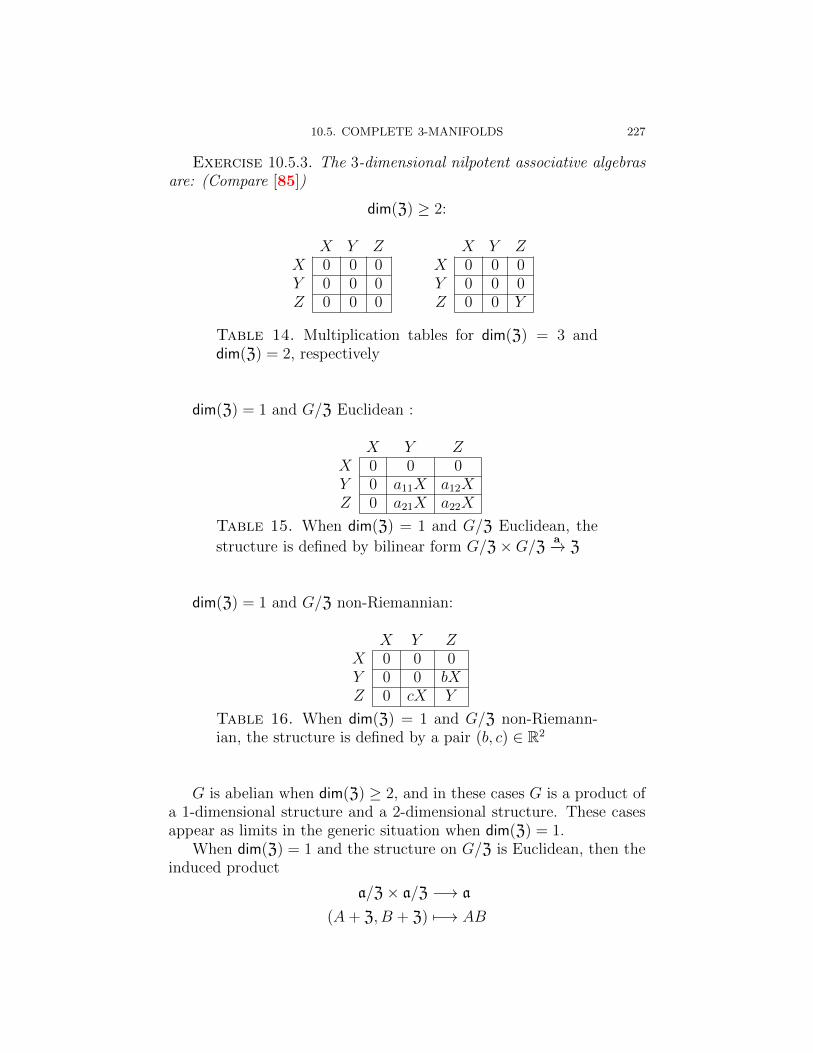
10.5. COMPLETE 3-MANIFOLDS 227
Exercise 10.5.3. The 3-dimensional nilpotent associative algebrasare: (Compare [85])
dim(Z) ≥ 2:
X Y ZX 0 0 0Y 0 0 0Z 0 0 0
X Y ZX 0 0 0Y 0 0 0Z 0 0 Y
Table 14. Multiplication tables for dim(Z) = 3 anddim(Z) = 2, respectively
dim(Z) = 1 and G/Z Euclidean :
X Y ZX 0 0 0Y 0 a11X a12XZ 0 a21X a22X
Table 15. When dim(Z) = 1 and G/Z Euclidean, the
structure is defined by bilinear form G/Z×G/Z a−→ Z
dim(Z) = 1 and G/Z non-Riemannian:
X Y ZX 0 0 0Y 0 0 bXZ 0 cX Y
Table 16. When dim(Z) = 1 and G/Z non-Riemann-ian, the structure is defined by a pair (b, c) ∈ R2
G is abelian when dim(Z) ≥ 2, and in these cases G is a product ofa 1-dimensional structure and a 2-dimensional structure. These casesappear as limits in the generic situation when dim(Z) = 1.
When dim(Z) = 1 and the structure on G/Z is Euclidean, then theinduced product
a/Z× a/Z −→ a
(A+ Z, B + Z) 7−→ AB

228 10. LIE GROUPS AND ALGEBRAS
defines a bilinear form R2 × R2 a−−→ Z ∼= R. Table 15 arises by takingX to be a generator of Z. The structure is abelian if and only if ais symmetric. In this case a is Euclidean if a = 0 and a product(dim(Z) = 2) when a is nonzero and degenerate.
When dim(Z) = 1 and the structure on G/Z is non-Riemannian, letX be generate Z, and extend to a basis X, Y, Z so that
(Z + Z)2 = Y
in the non-Riemannian quotient. The results are tabulated in Table 16.The structure is abelian if and only if b = c, and corresponds to theproduct structure (dim(Z) = 2) if and only if b = c = 0.
10.6. Fried’s counterexample to Auslander’s conjecture
Auslander’s conjecture [9] that a nilpotent simply transitive affinegroup contains central translations was disproved by Fried [83] by thefollowing 4-dimensional example.
A nilpotent Lie algebra is said to be filiform if it is “maximally non-abelian,” in the sense that its degree of nilpotence is one less than itsdimension. That is, a k-step nilpotent Lie algebra is filform if its dimes-nion equals k + 1. Fried’s example lives on the unique 4-dimensionalfiliform Lie algebra. (Curiously, Benoist’s example of an 11-dimensionalnilpotent Lie algebra admitting no faithful 12-dimensional linear rep-resentation — and hence no simply transitive affine actions — is afiliform Lie algebra.)
Let t, u, v, w ∈ R be real parameters. We parametrize the 4-dimensional filiform algebra as a semidirect sum
g := V0 oJ3 RT,
where V0 is a 3-dimensional abelian ideal with coordinates u, v, w andT acts by the 3-dimensional Jordan block
J3 :=
0 1 00 0 10 0 0.
That is, g admits a basis U, V,W, T subject to nonzero commutationrelations
[T, U ] = V, [T, V ] = W
and all other brackets between basic elements are zero.

10.6. CENTRAL TRANSLATIONS 229
We start with a simply transitive affine action, where U, V,W actby translations. The Lie algebra representation is:
A0(t, u, v, w) :=
0 0 0 0 t0 t 0 u
0 t v0 w
,
the group representation is:
A0(t, u, v, w) := expA0(t, u, v, w) :=
1 0 0 0 t1 t t2/2 u+ tv/2 + t2w/6
1 t v + tw/21 w
and a basis of left-invariant vector fields is:
X0 := ∂x, Y0 := ∂y, Z0 := ∂z + x∂y, W0 := ∂w + x∂z +x2
2∂y
with multiplication table:
X0 Y0 Z0 W0
X0 0 0 Y0 Z0
Y0 0 0 0 0Z0 0 0 0 0W0 0 0 0 0
Table 17. Complete affine structure on 4-dimensionalfiliform algebra
Then X0, Y0 are parallel vector fields and Z(g) is one-dimensional,spanned by Y0.
Now we deform using a parameter λ ∈ R, in the direction of theparallel vector field X0 = ∂x. Consider the affine representation A =Aλ,
A(t, u, v) = Aλ :=
0 −λw λ v −λu t0 t 0 u
0 t v0 w
Since

230 10. LIE GROUPS AND ALGEBRAS
a2 :=
0 −λ tw λ tv λ(−2uw + v2)0 t2 tv
0 tw0
,
a3 :=
0 −λ t2w 00 t2w
0
, A4 :=
0 −λt2w2
0
,
the general group element is:
exp(Aλ) :=
1 −λw λ v λ(− u+ tv/2− t2w/6
)t+ λ
(− uw + v2/2− t2w2/24
)
1 t t2/2 u+ tv/2 + t2w/61 t v + tw/2
1 w
.
The last column of this matrix is the developing map, and we can relatethe group coordinates to the affine coordinates, by:
x = t+ λ(− uw + v2/2− t2w2/24
)
y = u+ tv/2 + t2w/6
z = v + tw/2
w = w
A basis for right-invariant vector fields is:
T := ∂x+z∂y+w∂z, U := ∂y−λw∂x, , V := ∂z+λz∂x, W := ∂w−λy∂xwith U central.
I think the multiplication table for Fried’s example is:
X Y Z WX 0 0 Y ZY 0 0 0 λXZ 0 0 λX 0W 0 λX 0 0
Table 18. Fried’s counterexample to Auslander’s con-jecture on central translations

10.7. SOLVABLE 3-DIMENSIONAL ALGEBRAS 231
10.7. Solvable 3-dimensional algebras
If M3 is a closed manifold with complete affine structure, then Mis affinely isomorphic to a finite quotient of a complete affine solv-manifold, that is, a homogeneous space Γ\G, where G is a Lie groupwith a complete affine structure and Γ < G is a lattice. Equiva-lently, G admits a simply transitive affine action (corresponding toleft-multiplication). Necessarily G is solvable and we may assume thatG is simply-connected. Since G admits a lattice, it is unimodular. Reference for
solvability?We have already discussed the cases when G is nilpotent. Thereare two isomorphism classes of simply connected solvable unimodularnon-nilpotent Lie groups:
• The universal covering ˜Isom0(E2) of orientation-preserving isome-tries of of the group Isom0(E2) of orientation-preserving isome-tries of the Euclidean plane E2;• The identity component of the group Isom0(E1,1) of orientation-
preserving isometries of 2-dimensional Minkowski space.
Exercise 10.7.1. Prove that every lattice Γ < ˜Isom0(E2) containsa free abelian subgroup of finite index. In particular, Γ is a finite ex-tension of Z3 and is a 3-dimensional Bieberbach group.
Thus the only interesting remaining case for classifying completeaffine 3-manifolds occurs for the group Isom0(E1,1).
There are two isomorphism classes of complete left-invariant affinestructures on this group. One, which probably goes back to Auslander-Markus [7] is a group of isometries of a parallel Lorentzian metric; theother is due to Auslander [9] and corresponds to the simply transitiveaction, where λ ∈ R is a parameter (compare Fried-Goldman [85],Theorem 4.1):
(s, t, u)ρλ7−−−→
1 λesu λe−st s+ λtu0 es 0 t0 0 e−s u
When λ 6= 0, these actions are all affinely conjugate. The case λ = 0is the original flat Lorentzian structure.
Auslander notes that when λ 6= 0, the simply transitive actioncontains no translations.

232 10. LIE GROUPS AND ALGEBRAS
The corresponding left-invariant vector fields are:
X := ∂x
Y := ex−λyz(λz ∂x + ∂y
)
Z := e−x+λyz(λy ∂x + ∂z
)
with multiplication table:
X Y ZX 0 Y −ZY 0 0 λXZ 0 λX 0
10.8. Incomplete affine 3-manifolds
10.8.1. Parabolic cylinders. We can extend this structure tostructures on a 3-dimensional solvable Lie group G, which admits com-pact quotients. These provide examples of compact convex incom-plete affine 3-manifolds which are not properly convex, and nonradiant.Therefore Vey’s result that compact hyperbolic affine manifolds areradiant is sharp.
Further examples from the same group action give concave affinestructures on these same 3-manifolds.
The function:
A3 f−−→ R(x, y, z) 7−→ x− y2/2
is invariant under the affine R2-action defined by:
R2 U−−→ Aff(A3)
(t, u) 7−→ exp
0 t 0 00 0 0 t0 0 0 u
=
1 t 0 t2/20 1 0 t0 0 1 u
Under the 1-parameter group of dilations
R δ−→ Aff(A3)
s 7−→ exp
2s 0 00 s 00 0 −s
=
e2s 0 00 es 00 0 e−s

10.8. INCOMPLETE AFFINE 3-MANIFOLDS 233
the function f scales as:
f δ(s) = e2sf.
The group G ⊂ Aff(A3) generated by U(t, u)δ(s) (for s, t, u ∈ R) actssimply transitively on the open convex parabolic cylinder defined byf(x, y, z) > 0 as well as on the open concave parabolic cylinder definedby f(x, y, z) < 0. The corresponding left-invariant affine structure onthe Lie group G has a basis of left-invariant vector fields
X := f(x, y, z)∂x
Y := f(x, y, z)1/2(y∂x + ∂y
)
Z := f(x, y, z)−1/2∂z
with multiplication recorded in Table 19. The dual basis of left-invariant1-forms is:
X∗ := f(x, y, z)−1(dx− ydy) = −d log(f)
Y ∗ = f(x, y, z)−1/2dy
Z∗ = f(x, y, z)1/2dz
with bi-invariant volume form
X∗ ∧ Y ∗ ∧ Z∗ = f(x, y, z)−1dx ∧ dy ∧ dz.
This example is due to Goldman [91] providing examples of non-conicalconvex domains covering compact affine manifolds.
X Y ZX X Y/2 −Z/2Y 0 X 0Z 0 0 0
Table 19. Algebra corresponding to parabolic 3-dimensional halfspaces
10.8.2. Nonradiant deformations of radiant halfspace quo-tients. Another example arises from radiant suspensions. Namely,

234 10. LIE GROUPS AND ALGEBRAS
consider the radiant affine representation
Rn R2 ρα−−→ Aff(A3)
(s; t, u) 7−→ eαs exp
s 0 t0 −s u0 0 0
=
e(α+1)s 0 eαst
0 e(α−1)s eαsu0 0 eαs
depending on a parameter α ∈ R. When α 6= 0, the action is locallysimply transitive; the open orbits are the two halfspaces defined byz > 0 and z < 0 respectively. The vector fields
X := z(α+1)/α∂x
Y := z(α−1)/α∂y
Z := R = x∂x + y∂y + z∂z
correspond to a basis of left-invariant vector fields, with multiplicationrecorded in Table 20.
X Y ZX 0 0 XY 0 0 YZ
((α + 1)/α
)X
((α− 1)/α
)Y Z
Table 20. A radiant suspension
When α = ±1, then this action admits nonradiant deformations.Namely let β ∈ R be another parameter, and consider the case whenα = 1. The affine representation
Rn R2 ρβ−−→ Aff(A3)
(s; t, u) 7−→ exp
2s 0 0 00 0 0 βs0 0 s 0
· exp
0 0 t0 0 u0 0 0
=
e2s 0 e2st 00 1 u βs0 0 es 0

10.8. INCOMPLETE AFFINE 3-MANIFOLDS 235
maps
001
ρβ7−−−→
e2stu+ βses
=
xyz
so the group element with coordinates (s, t, u) corresponds to the pointwith coordinates
x = e2st
y = u+ βs
z = es
with inverse transformation:
s = log(z)
t = z−2x
u = y − β log(z)
Then the linear part Lρβ(s, t, u) corresponds to the matrixz2 0 x0 1 y − β log(z)0 0 z
whose columns base the left-invariant vector fields:
X := z2∂x
Y := ∂y
Z := x∂x +(y − β log(z)
)∂y + z∂z
Table 21 records their covariant derivatives.
X Y ZX 0 0 XY 0 0 YZ 2X 0 Z − βY
Table 21. Nonradiant Deformation

CHAPTER 11
Parallel volume and completeness
A particularly tantalizing open problem about closed affine man-ifolds is whether geodesic completeness (a geometric one-dimensionalproperty) is equivalent to parallel volume (an algebraic n-dimensionalproperty). This question was raised in 1963 by L. Markus [168] as a“Research Problem” in unpublished mimeographed lecture notes fromthe University of Minnesota (Problem 8, §6, p.58):
Question. Let M be a closed affine manifold. Then M is geodesi-cally complete if and only if M has parallel volume.
An affine manifold M has parallel volume if and only if it satisfiesany of the following equivalent conditions:
• The orientable double-covering of M admits a parallel volumeform (in the sense of §1.4.2 of Chapter 1);• M admits a coordinate atlas where the coordinate changes are
volume-preserving;• M admits a refined (SAff(A),A)-structure, where SAff(A) de-
notes the subgroup L−1(SL±(Rn)
)of volume-preserving linear
transformations;• For each φ ∈ π1(M), the linear holonomy L h(φ) has deter-
minant ±1.
11.1. The volume obstruction
Exercise 11.1.1. Prove the equivalence of the conditions stated inthe introduction to Chapter 11.
The last condition suggests a topological interpretation. The com-position of the linear holonomy representation L h with the logarithof the absolute value of the determinant
π1(M)Lh−−−→ GL(E)
|det |−−−−→ R+ log−−−→ Rdefines an additive homomorphsm νM ∈ Hom
(π1(M),R) ∼= H1(M ;R)
which we call the volume obstruction. M has parallel volume if andonly if νM = 0.
237

238 11. PARALLEL VOLUME AND COMPLETENESS
Exercise 11.1.2. Suppose that M is a manifold with zero first Bettinumber. Then every affine structure on M must have has parallel vol-ume.
One amusing corollary of this is that the only projective structureson the Q-homology 3-sphere S3
Q defined in §6.2.3.1 are complete affinestructures. Since S3
Q is covered by a 3-torus, the Markus conjecture forabelian holonomy (Smillie [201], Fried-Goldman-Hirsch [86]) impliesthat S3
Q must be complete, and must be covered by a complete affinenilmanifold (compare §11.2).
Exercise 11.1.3. Classify all the projective structures on S3Q.
Helmstetter’s theorem [114] that a left-invariant affine structure ona Lie group is complete ⇐⇒ right-invariant volume forms are parallelis an “infinitesimal version” of Markus’s conjecture. (Compare alsoGoldman-Hirsch [103].)
The plausibility of Markus’s question seems to be one of the mainbarriers in constructing examples of affine manifolds. A purely topolog-ical consequence of this conjecture is that a compact affine manifold Mwith zero first Betti number β1(M) is covered by Euclidean space: inparticular all of its higher homotopy groups vanish. Thus, if β1(M) = 0there should be no such structure on a nontrivial connected sum in di-mensions greater than two. (In fact no affine structure — or projectivestructure — is presently known on a nontrivial connected sum.) Joand Kim [130] resolve this question for convex affine manifolds.
11.2. Nilpotent holonomy
One of the first results on Markus’s question is its resolution in thecase the affine holomomy group is nilpotent.
The structure theory of affine structures on closed manifolds withnilpotent holonomy is relatively well understood, due to the work ofSmillie [201], Fried-Goldman-Hirsch [86] and Benoist [20, 23]. Smil-lie’s thesis develops the basic theory for affine structures with abelianholonomy, which Fried-Goldman-Hirsch extended to nilpotent holo-nomy, and Benoist extended to projective structures with nilpotenthonomy. The transition from nilpotent to solvable is much larger thanthe transition from abelian to nilpotent, and the next section discussesthe few results in the solvable non-nilpotent case, due to Serge Dupont.Compare also Fried’s classification of closed similarity manifolds in §.
The key technique in the discussion of nilpotent holonomy is thestructure theory of linear representations of nilpotent groups. The

11.2. NILPOTENT HOLONOMY 239
guiding principle is that nilpotence ensures a nontrivial center, pro-ducing lots of commuting transformations. Specifically, elements ofa nilpotent linear group have strongly compatible Jordan decomposi-tions, which leads to invariant geometric geometric structures for geo-metric manifolds with nilpotent holonomy. In another context whiswas used by Goldman [92] to give the first examples of 3-manifoldswithout flat conformal structures — for a geometric approach to thesealgebraic facts, see Thurston [212] and Ratcliffe [189].
The key to understanding nilpotent holonomy is the following alge-braic fact:
Theorem 11.2.1. Let V be a vector space over C and Γ < GL(V)a nilpotent group. Then ∃k ∈ N and Γ-invariant subspaces Vi < V fori = 1, . . . k such that
V =k⊕
i=1
Vi
and homomorphisms Γλi−−→ C∗ such that for each γ ∈ Γ and i =
1, . . . , k, the restriction γ − λiI to Vi is nilpotent. Furthermore thereexists a basis of Vi such that each restriction g|Vi is upper-triangularwith diagonal entry λi(g).
Corollary 11.2.2. Let A be an affine space over C and Γ <Aff(A). Then there exists a unique maximal Γ-invariant affine sub-space A1 < A such that the restriction of Γ to A1 is unipotent.
A1 is called the Fitting subspace in [86].Since Γ preserves the affine subspace A1, it induces an affine action
on the quotient space A/A1. Denote by V the vector space underlyingA. Since the affine action on A/A1 is radiant (it preserves the cosetA1 < A), we may describe A as an affine direct sum:
A = A1 ⊕ V1
where V1 ⊂ V is an L(Γ)-invariant linear subspace.
Theorem 11.2.3 (Smillie [201], Fried-Goldman-Hirsch [86]). LetM be a closed manifold with an affine structure whose affine holonomygroup Γ is nilpotent. Let A1 be its Fitting subspace and V1 its linearcomplement as above. Then ∃γ ∈ Γ such that the restriction γ|V1 is alinear expansion.
As in [201, 86], the Markus conjecture for nilpotent holnomy follows:
Corollary 11.2.4. Let M be a closed affine manifold whose affineholonomy group is nilpotent. Then M is complete if and only if it hasparallel volume.

240 11. PARALLEL VOLUME AND COMPLETENESS
Proof. Suppose M has parallel volume. Theorem 11.2.3 guaran-tees an element γ ∈ Γ whose linear part L(γ) is an expansion on V1.Thus V1 = 0, and A = A1, that is, Γ is unipotent. Apply Theorem 8.4.1to deduce that M is complete.
Conversely suppose M is complete, that is, the developing map
Mdev−−−→ A is a diffeomorphism. Then
M1 :=(dev−1(A1)
)/Γ ⊂ A/Γ ∼= M
is a closed affine submanifold and M1 →M is a homotopy-equivalence.Since both M1 and M are aspherical,
dim(A1) = dim(M1) = cd(Γ) = dim(M) = dim(A),
A1 = A and L(Γ) is unipotent, and hence volume-preserving. Thus Mhas parallel volume.
The geometric consequence of Theorem 11.2.3 is that the Γ-invariantdecomposition
A1 → A V1
defines two transverse affine foliations of M . The affine subspaces par-allel to A1 define the leaves of a foliation Fu of M . The leaves of Fu
are affine submanifolds of M with unipotent holonomy. The affine sub-spaces parallel to V1 define the leaves of a foliation FR of M . The leavesof FR are affine submanifolds of M with radiant affine structure.
Exercise 11.2.5. Suppose that M is closed. Show that each leaf ofFu is complete.
11.3. Smillie’s nonexistence theorem
Theorem 11.3.1 (Smillie [203]). Let M be a closed affine manifoldwith parallel volume. Then the affine holonomy homomorphism cannotfactor through a free group.
This theorem can be generalized much further — see Smillie [203] andGoldman-Hirsch [103].
Corollary 11.3.2 (Smillie [203]). Let M be a closed manifoldwhose fundamental group is a free product of finite groups (for example,a connected sum of manifolds with finite fundamental group). Then Madmits no affine structure.
Proof of Corollary 11.3.2 assuming Theorem 11.3.1.Suppose M has an affine structure. Since π1(M) is a free product offinite groups, the first Betti number of M is zero. Thus M has parallelvolume. Furthermore if π1(M) is a free product of finite groups, there

11.3. SMILLIE’S NONEXISTENCE THEOREM 241
exists a free subgroup Γ ⊂ π1(M) of finite index. Let M be the covering
space with π1(M) = Γ. Then the induced affine structure on M alsohas parallel volume contradicting Theorem.
Proof of Theorem 11.3.1. Let M be a closed affine manifoldmodeled on an affine space E, M
Π−→M a universal covering, and(M
dev−−→ E, πhol−→ Aff(E)
)
a development pair. Suppose thatM has parallel volume and that thereis a free group Π through which the affine holonomy homomorphism hfactors:
πφ−→ Π
h−−→ Aff(E)
Choose a graph G with fundamental group Π; then there exists a mapf : M −→ G inducing the homomorphism
π = π1(M)φ−→ π1(G) = Π.
By general position, there exist points s1, . . . sk ∈ G such that f istransverse to si and the complement G−s1, . . . , sk is connected andsimply connected. Let Hi denote the inverse image f−1(si) and letH = ∪iHi denote their disjoint union. Then H is an oriented closedsmooth hypersurface such that the complement M −H ⊂M has triv-ial holonomy. Let M |H denote the manifold with boundary obtainedby splitting M along H; that is, M |H has two boundary components
H+i , H
−i for each Hi and there exist diffeomorphisms H+
i
gi−→ H−i (gen-erating Π) such that M is the quotient of M |H by the identificationsgi. There is a canonical diffeomorphism of M −H with the interior ofM |H.
Let ωE be a parallel volume form on E; then there exists a parallelvolume form ωM on M such that
Π∗ωM = dev∗ωE.
SinceHn(E) = 0, there exists an (n−1)-form η on E such that dη = ωE.
For any immersion Sf−→ E of an oriented closed (n − 1)-manifold S,
the integral ∫
S
f ∗η
is independent of the choice of η satisfying dη = ωE. Since Hn−1(E),any other η′ must satisfy η′ = η + dθ and
∫
S
f ∗η′ −∫
S
f ∗η =
∫
S
d(f ∗θ) = 0.

242 11. PARALLEL VOLUME AND COMPLETENESS
Since M −H has trivial holonomy there is a developing map
M −H dev−−→ E
and its restriction to M −H extends to a developing map M |H dev−−→ Esuch that
dev|H+i
= h(gi) dev|H−iand the normal orientations ofH+
i , H−i induced fromM |H are opposite.
Since h(gi) preserves the volume form ωE,
d(h(gi)∗η) = d(η) = ω
and ∫
H+i
dev∗η =
∫
H+i
dev∗h(gi)∗η = −
∫
H−i
dev∗η
since the normal orientations of H±i are opposite. We now computethe ωM -volume of M :
vol(M) =
∫
M
ωM =
∫
M |Hdev∗ωE
=
∫
∂(M |H)
η =k∑
i=1
(∫
H+i
η +
∫
H−i
η
)= 0,
a contradiction.
One basic method of finding a primitive η for ωE involves a radiantvector field ρ. Since ρ expands volume, specifically,
dιρωE = nωE,
and
η =1
nιρωE
is a primitive for ωE. An affine manifold is radiant if and only if itpossesses a radiant vector field if and only if the affine structure comesfrom an (E,GL(E))-structure if and only if its affine holonomy has afixed point in E. The following result generalizes the above theorem:
Theorem 11.3.3 (Smillie). Let M be a closed affine manifold witha parallel exterior differential k-form which has nontrivial de Rhamcohomology class. Suppose U is an open covering of M such that foreach U ∈ U , the affine structure induced on U is radiant. Then dimU ≥k; that is, there exist k + 1 distinct open sets
U1, . . . , Uk+1 ∈ U

11.4. SIMILARITY MANIFOLDS 243
such that the intersection
U1 ∩ · · · ∩ Uk+1 6= ∅.(Equivalently the nerve of U has dimension at least k.)
A published proof of this theorem can be found in Goldman-Hirsch [103].Using these ideas, Carriere, dAl’bo and Meignez [47] have proved
that a nontrivial Seifert 3-manifold with hyperbolic base cannot havean affine structure with parallel volume. This implies that the 3-dimensional Brieskorn manifolds M(p, q, r) with
p−1 + q−1 + r−1 < 1
admit no affine structure whatsoever. (Compare Milnor [176].)There is a large class of discrete groups Γ for which every affine
representation Γ −→ Aff(E) is conjugate to a representation factoringthrough SL(E), that is,
Γ −→ SL(E) ⊂ Aff(E).
For example finite groups have this property, and the above theoremgives an alternate proof that the holonomy of a compact affine manifoldmust be infinite. Another class of groups having this property are theMargulis-superrigid groups, that is, irreducible lattices Γ in semisimpleLie groups G of R-rank greater than one (for example, SL(n,Z) forn > 2). Margulis proved [166] that every unbounded finite-dimensionallinear representation of Γ extends to a representation of G. It thenfollows that the affine holonomy of a compact affine manifold cannotfactor through a Margulis-superrigid group. However, since SL(n;R)
does admit a left-invariant RPn2−1-structure, it follows that if Γ ⊂
SL(n;R) is a torsion-free cocompact lattice, then there exists a compactaffine manifold with holonomy group Γ×Z although Γ itself is not theholonomy group of an affine structure.
11.4. Fried’s classification of closed similarity manifolds
Fried [81] gives a sharp classification of closed similarity manifolds;this was announced earlier by Kuiper [151], although the proof con-tains a gap. Later Reischer and Vaisman [215] proved this, using acompletely different set of ideas. Miner [180] extended Fried’s theoremto manifolds modeled on the Heisenberg group and its group of similar-ity transformations. Recently this has been exteneded to the boundarygeometry of any rank one symmetric space by Raphael Alexandre [3].Later, in §14.3, the ideas in Fried’s proof are related to Thurston’sparametrization of CP1-structures and the Kulkarni-Pinkall theory offlat conformal structures [156, 157].

244 11. PARALLEL VOLUME AND COMPLETENESS
11.4.1. Completeness versus radiance. Fried’s theorem is aprototype of a theorem about geometric structures on closed manifolds.Here X = En and G = Sim(En). Namely, Fried shows that a (G,X)-structure on a closed manifold M must reduce to one of two specialtypes, corresponding to subgeometries (G′, X ′) (G,X). Specifically,a closed similarity manifold must be one of the following two types:
• A Euclidean manifold where X ′ = X = En and
G′ = Isom(En) → Sim(En).
This is precisely the case when the underlying affine structureon M is complete;• A finite quotient of a Hopf manifold where X ′ = En\0 andG′ = Sim0(En) → Sim(En), the group of linear similarity (orconformal) transformations of En. The is precisely the casewhen the underlying affine structures is incomplete.
The complete case is easy to handle, since in that case Γ acts freely,and any similarity transformation which is not isometric must fix apoint. When M is incomplete, very little can be said in general, andthe compactness hypothesis must be crucially used.
Exercise 11.4.1. Prove that a complete similarity manifold is aEuclidean manifold, and diffeomorphic to a finite quotient of a productTr × En−r.
The other extreme — radiant similarity manifolds — were discussedin §6.5.2.1 of Chapter 6.
The recurrence of an incomplete geodesic on a compact manifoldguarantees a divergent sequence in the affine holonomy group Γ. Thisholonomy sequence converges to a singular projective transformationφ as in §2.6. The condition that Γ ⊂ Sim(En) strongly restricts φ; inparticular it has rank one or its limits are proximal, in that most pointsapproach a single point, which Fried shows must lie in En. From this hededuces radiance, and finds that the structure is modeled on En\0.We closely follow Fried’s proof (which we highly recommend reading),but insert more details and coordinate the notation with the rest ofthis document.
11.4.2. Canonical metrics and incompleteness. Choose a Eu-clidean metric gE on En; the pullback dev∗gE is a Euclidean metric on
M . UnlessM is a Euclidean manifold, this metric is not invariant under
π. rather it transforms by the scale factor homomorphism: πλh−−−→ R+:
(47) γ∗(dev∗gE
)= λ h(γ) dev∗gE.

11.4. SIMILARITY MANIFOLDS 245
defined in §1.4.1.
Exercise 11.4.2. Relate the scale factor λ h to the volume ob-struction νM .
Unless M is Euclidean, then dev∗gE is incomplete. Thus we assume
that (M, dev∗gE) is an incomplete Euclidean manifold with distance
function M × M dE−−→ R, non-bijective developing map Mdev−−−→ E and
nontrivial scale factor homomorphism π1(M)λ h−−−→ R+.
We begin with some general facts about an incomplete Euclideanmanifold N with trivial holonomy. We apply these facts to the case
when N is the universal covering M of a compact incomplete similaritymanifold M .
Exercise 11.4.3. Let N be a Euclidean manifold with trivial holo-
nomy. Choose a developing map Ndev−−−→ E. Let B ⊂ N be an open
subset. The following conditions are equivalent:
• B is an open ball in N , that is, ∃c ∈ N, r > 0 such thatB = Br(c).• B develops to an open ball in E, that is, ∃c ∈ E, r > 0 such that
the restriction dev|B is a diffeomorphism B −→ Br(c) ⊂ E;• B is the exponential image of a metric ball in the tangent space
TcN , that is, ∃c ∈ N, r > 0 such that the restriction Exp|Br(0c)is a diffeomorphism Br(0c) −→ B.
Under these conditions, the maps
Br(0c)Expc−−−−→ B
dev−−−→ Br
(dev(c)
)
are isometries with respect to the restrictions of the Euclidean metricson TcN , N and E, respectively.
Definition 11.4.4. A maximal ball in N is an open ball which ismaximal among open balls with respect to inclusion.
Exercise 11.4.5. A Euclidean manifold with trivial holonomy iscomplete (that is, is isomorphic to Euclidean space) if and only if noball is maximal.
Exercise 11.4.6. Suppose N is an incomplete Euclidean manifoldwith trivial holonomy.
• Let B ⊂ N be a maximal ball and let c be its center. Then Bis maximal among open balls centered at c.• Every open ball lies in a maximal ball.• Every x ∈ N is the center of a unique maximal ball B(x).

246 11. PARALLEL VOLUME AND COMPLETENESS
• For each x, not every point on ∂B(x) is visible from x.
Definition 11.4.7. Let N be an incomplete Euclidean manifoldwith trivial holonomy. For each x ∈ N , let R(x) <∞ be the radius ofthe maximal ball B(x) ⊂ N centered at x.
Exercise 11.4.8. The maximal ball B(x) = BR(x)(x). MoreoverR(x) is the supremum of r such that Br(0x) ⊂ Ex, where Ex ⊂ TxNdenotes the domain of Expx defined in §8.3 of Chapter 8.
Lemma 11.4.9. The function R is Lipschitz:
(48) |R(x)−R(y)| ≤ d(x, y)
if x, y ∈ N are sufficiently close. In particular R is continuous.
Proof. Suppose that x ∈ N and ε such that
ε < sup(R(x), R(y)
).
Choose r < R(x) so that Br(0x) ⊂ Ex. First we show that if d(x, y) < ε,then
(49) r < d(x, y) +R(y)
Choose u ∈ B(x) such that d(x, u) = r. Suppose that d(x, y) < ε.
Then closed ball Br(x) lies in the convex set B(x) which also containsy. Thus u ∈ ∂Br(x) is visible from y, whence
d(y, u) < R(y).
Thusr = d(x, u) ≤ d(x, y) + d(y, u) < d(x, y) +R(y),
proving (49). Taking the supremum over r yields:
R(x) < d(x, y) +R(y),
so R(x)−R(y) < d(x, y) if d(x, y) < ε. Similarly, symmetry of d implies
that R(x)−R(y) < d(x, y) if d(x, y) < ε which implies (48).
We return to the case that M is a compact incomplete similarity
manifold. Choose a universal covering NΠ−−→ M , a developing map
Ndev−−−→ E, and a holonomy representation π1(M)
h−−→ Sim(En). If
φ ∈ π1(M) is a deck transformation (also denoted Nφ−−→ N), then
φ(BR(p)
)is a maximal ball at φ(p), so:
(50) R(φp) = λ h(φ)R(p)
This leads to a natural conformal Riemannian structure on N whichdescends to a conformal Riemannian structure on M .

11.4. SIMILARITY MANIFOLDS 247
This will be the canonical Riemannian structure on a radiant sim-ilarity manifold. If M is closed and incomplete, then M is finitelycovered by a Hopf manifold M ′ homeomorphic to Sn−1 × S1. Theinduced Riemannian structure on M ′ is the Cartesian product of aspherical metric on Sn−1 with a Euclidean metric on S1. By (50), the
Riemannian metric g on M defined by:
(51) g(p) := R(p)−1dev∗gE
is π1(M)-invariant. Therefore g passes down to a Riemannian metricgM on M , that is, Π∗gM = g.
The Riemannian structure gM has the property that its unit ball ismaximal inside the domain E of the exponential map Exp. When M isclosed, even more is true:
Proposition 11.4.10. Let M be a compact incomplete similarity
manifold with universal covering NΠ−−→M . Then ∃ξ ∈ Vec(M) which
is Π-related to a vector field ξ ∈ Vec(N) such that:
• ‖ξ‖gM = ‖ξ‖g = 1;• The halfspace
Hx := v ∈ TxN | g(v, ξ) < 1lies in Ex for all x ∈ N .
In particularHx := Expx(Hx) ⊂ N
is a natural halfspace neighborhood of x.
By analyzing Hx, we shall prove that ξ is a radiant vector field andM is (covered by) a Hopf manifold. A key ingredient is a holonomysequence h(φij) ∈ Sim(En), where φij ∈ π1(M), which contracts to 0as j ∞ (Proposition 11.4.13). The proof of Proposition 11.4.10 willbe given in §11.4.4, following several preliminary lemmas needed in theproof.
11.4.3. Incomplete geodesics recur. Fried makes a detailed
analysis of an incomplete geodesic [0, 1)γ−−→ M . That is, γ(t) =
Exp(tv), where v ∈ TxM but tv ∈ Ex ⇐⇒ t < 1.Since M is compact (and [0, 1) isn’t compact), the path γ(t), ac-
cumulates. That is, for some sequence tn 1 a sequence γ(tn) ∈ Mconverges in M as n +∞. Denote
(52) p := limn→+∞
γ(tn)
Next, we use the recurrence of γ(t) to obtain a holonomy sequenceconverging to a singular projective transformation as in §2.6. To that

248 11. PARALLEL VOLUME AND COMPLETENESS
end, we pass to a specific universal covering space and a developingmap. Employ p ∈ M as a basepoint to define a universal covering
space MΠ−−→ M . The total space M comprises relative homotopy
classes of paths [0, T ]γ−−→M with γ(0) = p and the projection is:
MΠ−−→M
[γ] −→ γ(T )
The constant path defines a basepoint p ∈ M with Π(p) = p. The groupof deck transformations is π1(M, p) consisting of relative homotopyclasses of loops in M based at p.
Lift the incomplete geodesic [0, 1)γ−−→M to an incomplete geodesic
[0, 1)γ−−→ N so that
limn→+∞
γ(tn) = p
and let x := γ(0) be the initial endpoint of γ and v := γ′(0) ∈ TxNthe initial velocity.
Choose a developing map Mdev−−−→ En. A Euclidean metric tensor
gE on E induces a Euclidean metric tensor dev∗g on N . By rescaling, wemay assume that dev∗g(v, v) = 1. Denote the corresponding distance
function by N ×N d−−→ R. Choose a coordinate patch U 3 p such that
the restriction dev|U is injective, where U ⊂ M is the component ofΠ−1(U) containing p. Choose ε > 0 such that:
• Bε := Bε(0p) ⊂ Ep;• The ball B := Expp(Bε) lies in U ;
• ε < 12.
In particular, the restriction dev|B is injective.
Lemma 11.4.11. Let NR−−→ R+ be the radius function (defined in
11.4.7). Then
R(γ(t)
)= 1− t.
Exercise 11.4.12. Prove Lemma 11.4.11.
After possibly passing to a subsequence, (52) implies that γ(ti) ∈ B.Let
si := d(γ(ti), p
)
and [0, si]ηi−−→ M the unit-speed geodesic in B with ηi(0) = p and
ηi(si) = γ(ti). Lift ηi to
[0, si]ηi−−→ M
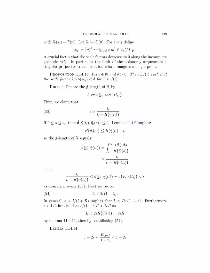
11.4. SIMILARITY MANIFOLDS 249
with ηi(si) = γ(ti). Let pi := ηi(0). For i < j define
φij :=[η−1j ? γ|[ti,tj ] ? ηi
]∈ π1(M, p).
A crucial fact is that the scale factors decrease to 0 along the incompletegeodesic γ(t). In particular the limit of the holonomy sequence is asingular projective transformation whose image is a single point.
Proposition 11.4.13. Fix i ∈ N and δ > 0. Then ∃J(i) such thatthe scale factor λ h(φij) < δ for j ≥ J(i).
Proof. Denote the g-length of ηi by
li := d(pi, dev γ(ti)
).
First, we claim that:
(53) ε >li
li +R(γ(ti)
) .
If 0 ≤ s ≤ si, then d(γ(ti), ηi(s)
)≤ li. Lemma 11.4.9 implies:
R(ηi(s)
)≤ R
(γ(ti) + li
so the g-length of ηi equals:
d(pi, γ(ti)
)=
∫ si
0
(ηi)∗ds
R(ηi(s)
)
≥ li
li +R(γ(ti)
)
Thusli
li +R(γ(ti)
) ≤ d(pi, γ(ti)
)= d(x, γi(ti)
)< ε
as desired, proving (53). Next we prove:
(54) li < 2ε(1− ti).In general, ε > l/(l + R) implies that l < Rε/(1 − ε). Furthermoreε < 1/2 implies that ε/(1− ε)R < 2εR so
li < 2εR(γ(ti)
)= 2εR
by Lemma 11.4.11, thereby establishing (54).
Lemma 11.4.14.
1− 2ε <R(pi)
1− ti< 1 + 2ε

250 11. PARALLEL VOLUME AND COMPLETENESS
Proof. Lemma 11.4.9 implies
|R(pi)−R(γ(ti)
)| ≤ d
(dev(pi), dev
(γ(ti)
)= li.
Lemma 11.4.11 and (54) together imply
|R(pi)− (1− ti)| < 2ε(1− ti).Now divide by 1− ti.
Lemma 11.4.15. For i < j,
R(xj)
R(pi)<
1 + 2ε
1− 2ε
1− tj1− ti
Proof. Apply Lemma 11.4.14 to obtain:
(55) R(xj) < (1 + 2ε)(1− tj)and
(1− 2ε)(1− ti) < R(pi)
that is,
(56)1
R(pi)<
1
(1− 2ε)(1− ti).
Multiplying (55) and (56) implies Lemma 11.4.15.
Since tj 1, for any fixed i, there exists J(i) such that j > J(i) implies
1 + 2ε
1− 2ε
1− tj1− ti
< δ.
Since xj = φij pi, (50) and (47) imply:
R(xj)
R(pi)= λ h(φij).
Now apply Lemma 11.4.15 to complete the proof of Proposition 11.4.13.
Recall from Exercise 2.6.6 of Chapter 2, that a sequence of similaritytransformations accumulates to either:
• The zero affine transformation (undefined at the ideal hyper-plane, otherwise constant;• A singular projective transformation of rank one, taking values
at an ideal point.
The contraction of scale factors (Proposition 11.4.13) implies that thesecond case cannot occur.

11.4. SIMILARITY MANIFOLDS 251
11.4.4. Existence of halfspace neighborhood. The contrac-tion of scale factors (Proposition 11.4.13) easily implies the existenceof halfspace neighborhoods (Proposition 11.4.10).
The proof uses the following elementary fact in Euclidean geometry:
Exercise 11.4.16. Let y ∈ En be a point and v ∈ TyEn ←→ Rn be atangent vector. Choosing coordinates, we may assume that Expy(v) = 0is the origin. Let St be a one-parameter family of homotheties approach-ing zero:
EnSt−−→ En
p 7−→ e−tp
Let B be the ball centered at y of radius R = ‖v‖:B := x ∈ En | d(y, x) < R
If tn ∞, then the union of Stn(B) is the halfspace H containing y
and orthogonal to the line segment←→y0:
H(y,0) := y + w | w · v < R.Let Ap denote the extension of dev Expp to TpN −→ A described
in Proposition 8.3.6.
Conclusion of proof of Proposition 11.4.10. Let x ∈ Mand lift to x ∈ N . Since M is incomplete, a maximal ball B(x) ⊂ Exexists, and denote its radius by R := R(x). Furthermore ∂B(x) con-tains a vector v of length R such that v /∈ Ex but tv ∈ Ex for |t| < 1.(Soon we shall see that v is unique, and will be the value ξ(x).)
Apply this construction to go from the incomplete geodesic
γ(t) := Expx(tv), (0 ≤ t < R),
inM to a holonomy sequence γij ∈ π1(M, p) satisfying Proposition 11.4.13.Define the halfspace
Hx := Y ∈ TxN | dev∗gE(v, Y ) < R= Y ∈ TxN | gN(v, Y ) < 1.
We show Hx ⊂ Ex. Suppose that Y is a tangent vector at x such that
dev∗gE(v, Y ) < R.
By Proposition 11.4.13, for j 1 and fixed i < j, the holonomy h(γij)is a very sharp contraction with rotational component close to theidentity — that is, it’s very close to a strong homothety about 0. ByExercise 11.4.16 above, (Dγij)x maps Y to a vector in Bγij(x) ⊂ Eγij(x)

252 11. PARALLEL VOLUME AND COMPLETENESS
for j i. Thus (Dγij)x(Y ) Is visible from γij(x) so Y is visible fromx, as claimed.
In particular every point in ∂B(x)\X lies in H(x), and thereforex uniquely determines X, so we write X =: ξ(x).
11.4.5. Visible points on the boundary of the halfspace.Bounding the halfspace Hx is the affine hyperplane
∂Hx := Y ∈ Tx | gN(v, Y ) < 1,which decomposes as the disjoint union of two subsets:
• The visible set ∂Hx ∩ Ex;• The invisible set ∂Hx \ Ex.
The invisible set is nonempty, since it contains ξ(x).
Lemma 11.4.17. The visible set ∂Hx ∩ Ex is nonempty.
Proof. Suppose every point of ∂Hx is invisible. Then Hx is aclosed subset of Ex. By construction, Hx is open and connected, soHx = Ex.
Thus the corresponding subset Hx = Exp(Htx) of N equals all ofN , so M is a quotient of a halfspace. The contradiction now followsfrom the following exercise.
Exercise 11.4.18. Let H ⊂ En be an open halfspace, and let Γ <Sim(En) be a discrete subgroup stablizing H and acting properly on H.Then the quotient Γ\H is not compact.
11.4.6. The invisible set is affine and locally constant. Thisuses the variation of Hx as x varies. The key is Lemma 1 of Fried [81],which says that if y = Expx(Y ), where Y ∈ ∂Hx∩Ex is a visible vector,then ξ(x) “is also invisible” from y. That is, the vector in TyN whoseparallel transport Py,x to x equals X ∈ Tx(N) is invisible from y.
Now apply the strong contraction γij to show that the halfplaneH(y) is moved closer and closer to 0. If it contains 0, then X = ξ(x)
is visible, a contradiction. If 0 /∈ H(y), then for j i, the maxi-mal ball B(y) is contained in a visible halfspace from x, contradictingmaximality. Thus ξ(x) is also invisible from y.
This shows that x uniquely determines the vector X, and the mapx 7−→ X is locally constant.
Exercise 11.4.19. Prove this map is affine and deduce that theinvisible subspace ∂Hx \ Ex is an affine subspace.

11.4. SIMILARITY MANIFOLDS 253
Now we return to the case that M is a closed affine manifold withholonomy covering space N .
Fried concludes th proof by observing now that the vector field cor-responds to an affine projection from the ambient affine space to theinvisible subspace ∂Hx \ Ex. Since it is invariant under deck transfor-mations it descends to a vector field on the compact quotient M .
Recall the divergence of a vector field (see §1.7.2) which measuresthe infinitesimal distortion of volume:
Exercise 11.4.20. The divergence of the vector field X equals dim∂Hx\Ex. Since M is closed, the vector field has divergence zero.
Thus ∂Hx ∩ Ex is a single point, and M is radiant, as desired.


CHAPTER 12
Hyperbolicity
The opposite of geodesic completeness is hyperbolicity in the senseof Vey [220, 219] and Kobayashi [142, 140], which is equivalent tothe following notion: An affine manifold M is completely incomplete ifand only if every affine map R −→M is constant, that is, M admits nocomplete geodesic. As noted by the author (see Kobayashi [142]), thecombined results of Kobayashi [142], Wu [230], and Vey [222, 221]imply:
Theorem. Let M be a closed affine manifold. Suppose that M iscompletely incomplete. Then M is a quotient of a properly convex cone.
I find it very striking that the two extreme cases for closed affine man-ifolds, the developing map is an embedding. That is, the developingmap for a complete affine manifold is a diffeomorphism, whereas thedevelping map for a completely incomplete affine manifold embeds theuniversal covering as a sharp convex cone.
In particular a completely incomplete affine manifold M is radiant.Furthermore it fibers over S1 as a radiant suspension of an automor-phism of a projective manifold of codimension one. Topological conse-quences are that the Euler characteristic χ(M) = 0 and the first Bettinumber b1(M) > 0.
Along the way we will also show that complete incompleteness isequivalent to the nonexistence of nonconstant projective maps R −→M .
This striking result uses intrinsic metrics for affine and projectivemanifolds, developed by Vey [220, 222, 219, 221] and Kobayashi [142,140]. Their constructions were in turn inspired by the intrinsic met-rics of Caratheodory and Kobayashi for holomorphic mappings betweencomplex manifolds.
We begin by discussing Kobayashi’s pseudometric for domains inprojective space, and then extend this construction to projective man-ifolds.
255

256 12. HYPERBOLICITY
12.1. The Kobayashi metric
To motivate Kobayashi’s construction, consider the basic case ofintervals in P1. (Compare the discussion in Exercise 2.5.7 on the cross-ratio.)
There are several natural choices to take, for example, the interval ofpositive real numbers R+ = (0,∞) or the open unit interval I = (−1, 1).
They relate via the projective transformation Iτ−−→ R+
x = τ(u) =1 + u
1− umapping −1 < u < 1 to 0 < x <∞ with τ(0) = 1. The correspondingHilbert metrics are given by
dR+(x1, x2) = log
∣∣∣∣x1
x2
∣∣∣∣(57)
dI(u1, u2) = 2
∣∣∣∣ tanh−1(u1)− tanh−1(u2)
∣∣∣∣.(58)
This follows from the fact that τ pulls back the parametrization corre-sponding to Haar measure on R+:
|dx|x
= |d log x|
to the Poincare metric on I:
dsI =2 |du|1− u2
= 2 |d tanh−1 u|.
A slight generalization of this will be useful in §12.2 in the proof ofthe projective Brody Lemma 12.2.18:
Exercise 12.1.1. Let r > 0 and denote by I(r) the open interval(−r, r) ⊂ R. Show that the diffeomorphism
I −→ I(r)
u 7−→ v = ru
maps 0 7→ 0, takes(ddu
)0
to r(ddv
)0, and, dually,
r dsI =2 r |du|1− u2
←−p 2r2 |dv|r2 − v2
.
Show that the infinitesimal form of the Hilbert metric on I(r) is:
dsI(r) =2 r |dv|r2 − v2
= 2 d tanh−1(v/r)
for v ∈ I(r) and v = r tanh(s/2).

12.1. THE KOBAYASHI METRIC 257
Exercise 12.1.2. Let x−, x+ ∈ R \ 0 be distinct. Show that theprojective map mapping
−1 7−→ x−
0 7−→ 0
1 7−→ x+
is given by:
t 7−→ 2(x−x+) t
(t+ 1)x− + (t− 1)x+
,
and a projective automorphism of I by
t 7−→ cosh(s)t+ sinh(s)
sinh(s)t+ cosh(s)=
t+ tanh(s)
1 + tanh(s)t
for s ∈ R.
In terms of the Poincare metric on I the Hilbert distance d(x, y) canbe characterized as an infimum over all projective maps I −→ Ω:
d(x, y) = inf
dI(a, b)
∣∣∣∣ f ∈ Proj(I,Ω), a, b ∈ I, f(a) = x, f(b) = y
We now define the Kobayashi pseudometric for any domain Ω and,more generally, any manifold with a projective structure (§12.2). Thisproceeds by a general universal construction forcing two properties:
• The triangle inequality : d(a, c) ≤ d(a, b) + d(b, c);• The projective Schwarz lemma: Projective maps do not in-
crease distance.
However, the resulting pseudometric may not be positive; indeed formany domains it is identically zero.
Let Ω ⊂ P be a domain and x, y ∈ Ω. A (projective) chain fromx to y is a sequence C of projective maps f1, . . . , fm ∈ Proj(I,Ω) andpairs ai, bi ∈ I, for i = 1, . . . ,m such that:
f1(a1) = x, f1(b1) = f2(a2), . . . ,
fm−1(bm−1) = fm(am), fm(bm) = y.
Denote the set of all projective chains from x to y by Chain(x y).Define length of a projective chain by:
`(C) =m∑
i=1
dI(ai, bi).
and the Kobayashi pseudodistance dKob(x, y):
dKob(x, y) = inf
`(C)
∣∣∣∣ C ∈ Chain(x y)
.

258 12. HYPERBOLICITY
The resulting function enjoys the following obvious properties:
• dKob(x, y) ≥ 0;• dKob(x, x) = 0;• dKob(x, y) = dKob(y, x);• (Triangle inequality) dKob(x, y) ≤ dKob(y, z) + dKob(z, x).• (Projective Schwarz lemma) If Ω,Ω′ are two domains in pro-
jective spaces with Kobayashi pseudometrics d, d′ respectivelyand
Ωf−−→ Ω′
is a projective map, then
d′(f(x), f(y)) ≤ d(x, y).
• The Kobayashi pseudometric on the interval I equals the Hilbertmetric on I.• dKob is invariant under the group Aut(Ω) consisting of all collineations
of P preserving Ω.
Proposition 12.1.3 (Kobayashi [142]). Let Ω ⊂ P be properlyconvex. If x, y ∈ Ω, then
dHilb(x, y) = dKob(x, y)
Corollary 12.1.4. The function dHilb : Ω×Ω −→ R is a completemetric on Ω.
Proof of Proposition 12.1.3. Let x, y ∈ Ω be distinct pointsand let l =←→xy be the line incident to them. Now
dHilbΩ (x, y) = dHilb
l∩Ω(x, y) = dKobl∩Ω(x, y) ≤ dKob
Ω (x, y)
by the Schwarz lemma applied to the projective map l ∩Ω → Ω. Forthe opposite inequality, let S be the intersection of a supporting hyper-plane to Ω at x∞ and a supporting hyperplane to Ω at y∞. Projectionfrom S to l defines a projective map
ΠS,lΩ −→ l ∩ Ω
which retracts Ω onto l ∩ Ω. Thus
dKobΩ (x, y) ≤ dKob
l∩Ω(x, y) = dHilbΩ (x, y)
(again using the Schwarz lemma) as desired.
Corollary 12.1.5. Line segments in Ω are geodesics. If Ω ⊂P is properly convex, x, y ∈ Ω, then the chain consisting of a singleprojective isomorphism
I −→←→xy ∩ Ω
minimizes the length among all chains in Chain(x y).

12.2. KOBAYASHI HYPERBOLICITY 259
Exercise 12.1.6. Prove that the geodesics in Ω with respect to thismetric are straight lines.
An affine (respectively projective) manifold is hyperbolic if the Kobayashipseudometric dKob is a metric, that is, if dKob(x, y) > 0 for x 6= y. Acompact affine manifold M is hyperbolic if and only if if it is a quo-tient of a properly convex cone; a compact projective manifold is hy-perbolic if and only if it is a quotient of a properly convex domainin projective space. The tameness of developing maps of hyperbolicaffine and projective structures suggests, when the pseudometric dKob
fails to be a metric, that dKob may provide a useful tool to understandpathological developing maps.
12.2. Kobayashi hyperbolicity
Now we discuss intrinsic metrics on affine and projective manifolds.The case of domains was discussed in §??.
Recall from §12.1 the open unit interval I = (−1, 1) with Poincaremetric
gI :=4 du2
(1− u2)2=(dsI
)2
,
where
dsI =√
gI :=2 du
1− u2= d
(2 tanh−1(u)
)
defines the associated norm on the tangent spaces. As in §12.1, the nat-ural parameter s for arc length on I relates to the Euclidean coordinateu on I ⊂ R by:
u = tanh(s/2).
For projective manifolds M , one defines a “universal” pseudometric
M ×M dKobM−−−→ R
such that affine (respectively projective) maps I→M are distance non-increasing with respect to dsI. This generalizes the Kobayashi metricfor projective domains discussed in §12.1.
The definition of dKobM for an arbitary RPn-manifold M enforces
the triangle inequality and Schwarz lemma by taking the infimum ofgI-distances over chains in M , as in §12.1. Recall that if x, y ∈ M ,a (projective) chain from x to y is a sequence of projective mapsf1, . . . , fm ∈ Proj(I,M) and pairs ai, bi ∈ I, for i = 1, . . . ,m suchthat:
f1(a1) = x, f1(b1) = f2(a2), . . . ,
fm−1(bm−1) = fm(am), fm(bm) = y.

260 12. HYPERBOLICITY
Denote the set of all chains from x to y by Chain(x y) and definelength:
Chain(x y)`−−−→ R≥0
(((a1, b1), f1
), . . . ,
((am, bm), fm
))7−→
m∑
i=1
dI(ai, bi),
where dI is the distance function on the Riemannian 1-manifold (I, gI).Now define the Kobayashi pseudodistance dKob(x, y) as:
M ×M dKob
−−−→ R≥0
(x, y) 7−→ inf
`(C)
∣∣∣∣C ∈ Chain(x y)
.
just as in as in §12.1. Just as in the case of domains, dKob satisfies thetriangle inequality and the Projective Schwarz lemma:
Lemma 12.2.1 (Projective Schwarz Lemma). Projective maps donot increase pseudodistances: If x, y ∈ N , and f ∈ Proj(N,M), then
dKobM
(f(x), f(y)
)≤ dKob
N
(x, y).
Definition 12.2.2. Let M be an RPn-manifold. Then M is (pro-jectively) hyperbolic if and only if dKob
M > 0, that is, if(M, dKob
M
)is a
metric space. Say that M is complete hyperbolic if if the metric space(M, dKob
M
)is complete.
.
12.2.1. Complete hyperbolicity and convexity. The follow-ing convexity theorem is due, independently, to Vey [219, 220], andKobayashi [142], from somewhat different viewpoints. We closely fol-low Kobayashi [142]; see also [140, 141].
Proposition 12.2.3. Let M be a complete hyperbolic projectivemanifold. Then M is properly convex, that is, M is isomorphic to aquotient of a properly convex domain by a discrete group of collineations.
The proof will be based on the following fundamental compact-ness property of projective maps (compare Vey [220], Proposition IV,Chapitre II):
Lemma 12.2.4. Suppose that M,N are projective manifolds, whereM is complete hyperbolic. Let p ∈ N and K ⊂⊂M . Then
Projp,K(N,M) :=f ∈ Proj(N,M)
∣∣ f(p) ∈ K
is compact.Do we need Ncompact?

12.2. KOBAYASHI HYPERBOLICITY 261
Proof. Apply the Projective Schwarz Lemma 12.2.1 to Lemma C.2.1(Theorem 3.1 of Chapter V of Kobayashi [143]), discussed in Appen-dix C.
Proof of Proposition 12.2.3. We show that M is geodesicallyconvex, that is, if ∀p, q ∈M , every path p q is relatively homotopicto a geodesic path from p to q. We may assume that M is simplyconnected.
For p ∈ M , let M(p) ⊂ M be the union of geodesic segments inM beginning at p. Exercise 8.3.4 implies M(p) is open. Since M isconnected, it suffices to show M(p) is closed.
Suppose that qn ∈ M(p) for n = 1, 2, . . . be a convergent sequencein M with q = limn→∞ qn. We show that q ∈M(p).
Let 0 < a < 1 and fn ∈ Proj(I,M) with fn(0) = p and fn(a) = qn.Lemma 12.2.4 guarantees a subsequence of fn converging to a projectivemap f ∈ Proj(I,M) with f(0) = p. Then
q = limn→∞
qn = limn→∞
fn(a) = f(a) ∈M(p)
and M(p) is closed, as desired.
12.2.2. The infinitesimal form. Kobayashi’s pseudometric dKob
has an infinitesimal form ΦKob defined by a function TMΦKob
−−−→ R.That is, dKob(p, q) is the infimum of the pseudolengths
`(γ) :=
∫
γ
ΦKob(γ′)
over piecewise C1 paths pγ q. For x ∈M and ξ ∈ TxM , define:
ΦKob(ξ) :=(59)
inf
|dsI(v)|
∣∣∣∣ f ∈ Proj(I,M), f(u) = x, (Df)u(v) = ξ
where u ∈ I and dsI(v) denotes the norm of v ∈ TuI with respect tothe Poincare metric (dsI)
2 on I.
Exercise 12.2.5. For affine manifolds, completeness is equivalentto ΦKob ≡ 0. For a Hopf manifold, dKob ≡ 0 but ΦKob 6= 0. IndeedΦKob(R) = 1 where R is the radiant vector field.
Exercise 12.2.6. Show that ΦKob is homogeneous of degree one,that is,
ΦKob(rξ) = rΦKob(ξ)
for r ≥ 0. Deduce that `(γ) is independent of the parametrization of γ.

262 12. HYPERBOLICITY
Proposition 12.2.7. ΦKob is upper semicontinuous.
Recall that a function Xf−−→ R is upper semicontinuous at x ∈ X if
and only if ∀ε > 0,
f(y) < f(x) + ε
for y in an open neighborhood of x. That is, the values of f cannot“jump down” in limits.
limn→∞
f(ξn) ≤ f(
limn→∞
ξn)
for convergent sequences ξn. Equivalently, f is a continuous mappingfrom X to R, where R is given the topology whose open sets are in-tervals (−∞, a) where a ∈ R. The indicator function of a closed set isupper semicontinuous. Semicontinuous functions are further discussedin Appendix D.
Proof of Proposition 12.2.7. Let x ∈ M and ξ ∈ TxM andwrite
ΦKob(ξ) = k.
Let ε > 0. Then ∃f ∈ Proj(I,M) with f(u) = x, and v ∈ TuI with(Df)u(v) = ξ and
‖v‖ < k + ε/2.
Lift f to f ∈ Proj(I, M) and extend f to F ∈ Proj(B, M). Let ‖‖Bthe corresponding norm for the intrinsic metric on B defined in §3.2.5.We may assume that ‖ξ‖B = ‖ξ‖. Then an open neighborhood N of
ξ ∈ TM exists so that if ξ′ ∈ N , then:
• ξ′ ∈ Tx′M where x′ lies in the image F (B) ⊂ M ;
• ‖(DF )−1(ξ′)‖B < k + ε.
Since projective maps do not increase distance, ‖ξ′‖M < k + ε, asdesired.
Corollary 12.2.8 (Proposition 5.16 of Kobayashi [142]). If M is
a complete hyperbolic projective manifold, then TMΦKob
−−−−→ R is con-tinuous.
The proof uses the following lemma (Lemma 5.17 of Kobayashi [142]),stating that the infimum in the definition of ΦKob is actually achieved.
Lemma 12.2.9. Suppose M is complete hyperbolic and ξ ∈ TpM .Then ∃f ∈ Proj(I,M) and v ∈ T0I with f(0) = p and (Df)0(v) = ξsuch that ΦKob(ξ) = ‖v‖.

12.2. KOBAYASHI HYPERBOLICITY 263
Proof. Lemma 12.2.4 implies that the subset of Proj(I,M) com-
prising projective maps If−−→ M with f(0) = p is compact. Thus the
set of ‖(Df)−1(ξ)‖ is a compact subset of R+, so its infimum ΦKob(ξ)is positive.
Proof of Corollary 12.2.8. Suppose, for k = 1, 2, . . . , thatξk ∈ TpkM , defines a sequence converging to ξ∞ ∈ Tp∞M . We showthat limk→∞ΦKob(ξk) = ΦKob(ξ∞).
Proposition 12.2.7 (semicontinuity of ΦKob) implies that
(60) ΦKob(ξ∞) ≥ limk→∞
ΦKob(ξk),
so it suffices to show that ΦKob(ξ∞) ≤ limk→∞ΦKob(ξk).The above lemma guarantees fk ∈ Proj(I,M) with fk(0) = pk and
vk := (Dfk)−1(ξk) ∈ T0I
such that ΦKob(ξk) = ‖vk‖. By (60), vk contains a convergent subse-quence, and let v∞ := limk→∞ vk. Lemma 12.2.4 guarantees that bypassing to a further subsequence, we may assume that fk convergesto f∞ ∈ Proj(I,M) with f∞(0) = p∞ and Df∞(v∞) = ξ∞. By thedefinition of ΦKob,
ΦKob(ξ∞) ≤ ‖v∞‖ = limk→∞‖vk‖ = lim
k→∞ΦKob(ξk)
as desired.
Exercise 12.2.10. Find an example of a projectively hyperbolic do-main for which ΦKob is not continuous.
Exercise 12.2.11. Find an example of a domain Ω for which:
• ΦKob(ξ) <∞ for all nonzero ξ ∈ TΩ;• Ω contains no complete geodesic rays.
Theorem 12.2.12. ΦKob is the infinitesimal form of the Kobayashipseudometric dKob
M , that is,
dKobM (x, y) = inf
∫ b
a
ΦKob(γ′(t)
)dt
∣∣∣∣ γ ∈ Path(x y)
where Path(x y) denotes the set of piecewise C1 paths [a, b]γ−−→ M
with γ(a) = x, γ(b) = y.
Since semicontinuous functions are bounded on compact sets (Ex-ercise D.2.3) and measurable (Exercise D.1.2), the above integral iswell-defined.

264 12. HYPERBOLICITY
Proof of Theorem 12.2.12. Define
δKob(p, q) := inf
∫ b
a
ΦKob(γ′(t)
)dt
∣∣∣∣ γ ∈ Path(p q)
We must prove that δKob = dKob.To prove δKob ≤ dKob, note that every chain C ∈ Chain(x y)
determine a piecewise C1 path γC ∈ Path(p q). Since gI is theinfinitesimal form of dI, the path γC has shorter length than the chainC, that is, their lengths satisfy `(γC) ≤ `(C). Taking infima impliesδKob ≤ dKob as desired.
We prove δKob ≥ dKob. Suppose that γ ∈ Path(p q) as above.Suppose ε > 0. We seek a chain C ∈ Chain(p q) such that
(61) `(C) ≤ `(γ) + ε.
Proposition 12.2.7 implies that the function
[a, b]φ−−→ R
u 7−→ ΦKob(γ′(t)
)
is upper semicontinuous. Exercise D.2.3 implies φ is bounded fromabove. Apply Proposition D.2.4 to conclude that φ is the limit ofa monotonically decreasing sequence of nonnegative continuous func-tions.
Apply Lebesgue’s monotone convergence theorem (Rudin [193],1.26)
to find a continuous function [a, b]h−−→ R such that:
φ(t) < h(t) for a ≤ t ≤ b(62) ∫
[a,b]
h < `(γ) + ε.(63)
for a ≤ t ≤ b.We claim that for each s ∈ [a, b],
(64)
∫ t
s
φ(u) du ≤ (1 + ε)h(s) |s− t|
for t in an interval Is centered at s.To this end, first assume that γ is C1; We choose the open neigh-
borhood Is of s in three steps:First, choose a convex ball Ws containing γ(s), so that γ(t) ∈ Ws
for t ∈ Is. Let ft ∈ Proj(I,M) extend the geodesic in Ws joining γ(s)to γ(t). Then (62) implies that ‖(Dft)
−1(γ′(s)
)‖ < h. Since γ is C1,
(65) ‖(Dft)−1(γ′(t)
)‖ < h
for t sufficiently near s.

12.2. KOBAYASHI HYPERBOLICITY 265
Next, choose Is so that (65) holds for t ∈ Is. This implies that
(66)
∫ t
s
h(u)du ≤ (1 + ε)h(s) |s− t|
for t sufficiently near s.Finally, choose Is so that (66) holds for t ∈ Is.Combining (66) with (62) implies
∫ t
s
φ(u)du <
∫ t
s
h(u)du ≤ (1 + ε)h(s) |s− t|,
establishing the claim when γ is C1. Extending (66) to the case thatγ is only piecewise C1 is a routine exercise.
Continuing to follow Wu [230]), we pick up the argument of Roy-den [192]. Let η > 0 be a Lebesgue number for the open coverIs | s ∈ I of I, that is, every closed interval of length < η lies insome Is. (For the reader’s convenience, a proof of the existence of theLebesgue number is given in Appendix C.3.) Thus there exists a sub-division a = t0 < t1 < · · · < tk = b exists with ti − ti−1 < η; let si besuch that [ti−1, ti] ⊂ Isi . Continuity of h and (63) imply
(67)k∑
i=1
h(si)(ti − ti−1) <
∫ b
a
h(u) < `(γ) + ε.
By (64),
dKob(γ(si), γ(si−1)
)≤ dKob
(γ(si), γ(s−1)
)+ dKob
(γ(si), γ(s−1)
)
≤ (1 + ε)(h(si)(si − ti) + h(si−1)(ti − si−1)
)
Apply (66) and (67), obtaining:
dKob(p, q) ≤k∑
i=1
dKob(γ(si), γ(si−1))
≤k∑
i=1
h(si)(ti − ti−1)
< `(γ) + ε.
Now the chain C ∈ Chain(p q) defined by:
C :=((
(s1, s2, f1
), . . . , (sk−1, sk), fk
))
has length
`(C) =k−1∑
i=1
dKob(γ(si, si+1)
)

266 12. HYPERBOLICITY
and (61) follows. Since ε > 0 is arbitrary, dKob(p, q) ≤ `(γ) ≤ δ asdesired.
Wu [230]) actually proves a much stronger statement, valid foraffine connections which are not necessarily flat. His proof is based onthe analog for the Kobayashi pseudometric for complex manifolds, dueto Royden [192].
Closely related is the universal property of ΦKob among infinitesimalpseudometrics for which projective maps are infiniteimally nonincreas-ing (Kobayashi [142], Proposition 5.5):
Exercise 12.2.13. Let M be an RPn-manifold and MΦ−−→ R≥0 a
function such that ∀f ∈ Proj(I,M)
Φ((Df)a(ξ)
)≤ ‖ξ‖a,
where −1 < a < 1 and ξ ∈ TaI. Then Φ ≤ ΦKob.
12.2.3. Completely incomplete manifolds.
Exercise 12.2.14. Let M be a affine manifold. Suppose that everygeodesic ray is incomplete. Then M is noncompact.
Theorem 12.2.15. Suppose that M is an RPn-manifold. ThendKobM > 0 if and only if every projective map R −→M is constant.
More specifically, we prove (following Kobayashi [142]):
Proposition 12.2.16. Let M be a projective manifold, p ∈M andξ ∈ TpM . Suppose ΦKob(ξ) = 0. Then ∃f ∈ Proj(R,M) with f(0) = pand f ′(0) = ξ.
Since ΦKob(p, ξ) = 0, there is a sequence jm ∈ Proj(I,M) withjm(0) = p and a sequence am > 0 with am decreasing, am 0 suchthat the differential (Djm)0 of jm at 0 ∈ I maps:
T0I(Djm)0−−−−−→ TpM
am
(d
du
)
0
7−→ ξ.
Let rm = 1/am so that
(68)
(d
du
)
0
(Djm)07−−−−−→ rmξ
with rm +∞ monotonically.As in Exercise 12.1.1, let I(r) denotes the open interval (−r, r) ⊂ R.
ThenI(r1) ⊂ I(r2) ⊂ · · · ⊂ I(rm) ⊂ · · · ⊂ R

12.2. KOBAYASHI HYPERBOLICITY 267
and⋃∞m=1 I(rm) = R.
The strategy of the proof is to reparametrize the maps jm to obtaina subsequence of projective maps
hm ∈ Proj(I(rm),M
),
such that the restriction of hm to hl equals hl for l ≤ m.First renormalize jm to a projective map fm ∈ Proj(I(rm),M):
I(rm)fm−−−→M
u 7−→ jm(u/rm)
Lemma 12.2.17. The differential (Dfm)0 of fm at 0 maps the tan-gent vector
(ddu
)0∈ T0
(I(rm)
)to ξ.
Proof. fm equals the composition of If−−→ M with the contreac-
tion
I(rm) −→ I
u 7−→ u/rm
0 7−→ 0
whose differential at 0 is multiplication by (rm)−1. Now apply the chainrule and (68).
Next reparametrize the maps fm using the following analog of Brody’sreparametrization lemma for holomorphic mappings (Brody [39]), whoseproof is given later.
As in Exercise 12.1.1, the infinitesimal norm for I(r) equals:
dsI(r) =2r|du|r2 − u2
,
a function on TI(r). As in Kobayashi [142] 1 choose a Riemannianmetric g on M such that g(ξ) = 1. The corresponding norm on TMis√
g and pulls back to a norm f ∗√
g on TuI(r). Then there is acontinuous function
I(r)Wf−−−→ R+
such that
(69) f ∗√
g(u) = Wf (u) dsI(r)(u).
Lemma 12.2.18 (Reparametrization Lemma). Let M be an pro-jective manifold, p ∈ M and ξ ∈ TpM nonzero. Suppose that f ∈Proj(I(r),M) with f(0) = p and f ′(0) = ξ. Choose c such that Wf (0) >
1Remark 5.27 after Theorem 5.22, pp.145–146

268 12. HYPERBOLICITY
c > 0. Then ∃a, b with 0 < a < 1 and b ∈ Aut(I(r)
)such that
h ∈ Proj(Ir,M) defined by:
h(u) := f(ab(u)
)
satisfies
• Wh(u) ≤ c;• Wh(0) = c,
where Wh is defined in (69)
Conclusion of proof of Proposition 12.2.16 assuming Lemma 12.2.18.Applying Lemma 12.2.18 to fm, ∃hm ∈ Proj(I(rm),M) and cm > 0 suchthat
(70) Whm(u) ≤ cm and Whm(0) = c
and the image of fm contains the image of hm.Denote the restriction of hm to Irl by hl,m. Equation (70) implies
that, for each l ∈ N, the family
Fl := hl,m | m ≥ lis equicontinuous.
We construct the projective map h ∈ Proj(R,M) by consecutiveextensions hl ∈ Proj(Irl ,M) to Irl ⊃ Irl−1
as follows.Begining with l = 1, the Arzela-Ascoli theorem guarantees a con-
vergent subsequence h1,m in Proj(Ir1 ,M). Write
h1 = limm→∞
h1,m ∈ Proj(Ir1 ,M).
Suppose inductively that hl ∈ Proj(Irl ,M) has been defined such thathl extends hk for all k ≤ l. Since Fl is equicontinuous, the Arzela-Ascolitheorem guarantees a convergent subsequence of hl,m. Define
hl := limm→∞
hl,m.
The value of h∗m√
g at u = 0 equals 2c du 6= 0. Since this is thevalue of h∗
√g = h∗l
√g at u = 0, the map h is nonconstant. This
concludes the proof of Proposition 12.2.16 assuming Lemma 12.2.18.
Proof of Lemma 12.2.18. For 0 ≤ t ≤ 1, consider the projec-tive map
I(r)ft−−→M
u 7−→ f(tu).

12.3. HESSIAN MANIFOLDS 269
Then the corresponding function Wt := Wft
(defined as in (69)
)
I(r)Wt−−−→ R+
satisfies the following elementary properties, whose proofs are left asexercises:
(71) Wt(u) = Wf (tu)t(r2 − u2)
r2 − t2u2
(72) Wt(u) ≥ 0 and Wt(u) = 0⇐⇒ t = 0.
(73) limu→±r
Wt(u) = 0.
The functionA(t) := sup
u∈I(r)
Wt(u)
of t ∈ [0, 1] satisfies the following elementary properties, whose proofsare also left as exercises:
• A(t) ≤ ∞• [0, 1]
A−−→ R+ is continuous.• A is monotone-increasing.
Furthermore A(0) = 0 and A(1) = c, so the Intermediate Value Theo-rem guarantees ∃a ∈ [0, 1] such that A(a) = c. Thus
c = supu∈I(r)
Wa(u).
By (73), Wa assumes its maximum on u0 ∈ I(r); let b ∈ Aut(I(r)
)take
0 to u0. The proof of Lemma 12.2.18 is complete.
12.3. Hessian manifolds
When M is affine, then Corollary 4.3.2 implies that M is a quotientof a properly convex cone Ω by a discrete group of collineations actingproperly on Ω. In addition to the Hilbert metric, Ω enjoys the naturalRiemannian metric introduced by Vinberg [223], Koszul [147, 146,150, 149] and Vesentini [218]. (Compare §??.) In particular Koszuland Vinberg observe that this Riemannian structure is the covariantdifferential ∇ω of a closed 1-form ω. In particular ω is everywherenonzero, so by Tischler [213], M fibers over S1.
This implies Koszul’s beautiful theorem [150] that the holonomymapping hol (described in Chapter 7,§7.2) embeds the space of con-vex structures onto an open subset of the representation variety. This

270 12. HYPERBOLICITY
has recently been extended to noncompact manifolds by Cooper-Long-Tillmann [62].
Hyperbolic affine manifolds closely relate to Hessian manifolds. Ifω is a closed 1-form, then its covariant differential ∇ω is a symmetric2-form. Since closed forms are locally exact, ω = df for some function;in that case ∇ω equals the Hessian d2f . Koszul [150] showed thathyperbolicity is equivalent to the existence of a closed 1-form ω whosecovariant differential ∇ω is positive definite, that is, a Riemannianmetric. More generally, Shima [199] considered Riemannian metrics onan affine manifold which are locally Hessians of functions, and provedthat such a closed Hessian manifold is a quotient of a convex domain,thus generalizing Koszul’s result.
We briefly sketch some of the ideas in Koszul’s paper. We rec-ommend Shima’s book [199] for a very accessible and comprehensiveexposition of these and related ideas.
Let (M,∇) be an affine manifold with connection ∇. Let x ∈ Mand Ex ∈ TxM denote the domain of exponential map as in §8.3.1. Forξ ∈ TxM , let
λ(ξ) := supt ∈ R | tξ ∈ Ex ∈ (0,∞],
so that the intersection of the line Rξ with Ex equals(−λ(−ξ), λ(ξ)
)ξ.
Suppose that ω is a closed 1-form as above, such that the covariantdifferential ∇ω > 0. Koszul’s theory is based on the two lemmas below.For notational simplicity, write
(− λ(−ξ), λ(ξ)
) γ−−→M
t 7−→ Expx(tξ)
for the maximal geodesic with velocity ξ = γ′(0) at time t = 0. Observethat for any −λ(−ξ) < t < λ(ξ), the velocity vector at time t is
γ′(t) = Pγt(ξ)
where xγt γ(t) is the restriction of γ and
TxMPγt−−−→ Tγ(t)M
denotes parallel transport along γt. The two basic lemmas are:
Lemma 12.3.1. If ω(ξ) > 0, then λ(ξ) <∞.Lemma 12.3.2. If λ(ξ) <∞, then
∫ λ(ξ)
0
ω(γ′(t)
)dt = +∞.

12.3. HESSIAN MANIFOLDS 271
The role of positivity is apparent from the simple 1-dimensionalexample when M = R+ ⊂ R. To develop intuition for these conditions,we work out these lemmas in the basic example when M = R+ ⊂ R.
First we show (Lemma 12.3.1) that that ω(ξ) > 0 implies the thegeodesic ray γ is incomplete. The cone Ω∗ dual to M consists of allψ > 0 and the characteristic function is
Mf−−→ R
x 7−→∫
Ω∗e−ψxdψ =
∫ ∞
0
e−ψxdψ =1
x
and the logarithmic differential equals
ω = d log f = −dxx.
If ξ = y0∂x ∈ Tx0M and ξ 6= 0, then γ(t) = x0 + ty0 and
λ(ξ) =
−x0/y0 if y0 < 0
∞ if y0 > 0
Similarly
ω(γ′(t)
)=(− dx/(x0 + ty0)
)(y0∂x
∣∣x=x0+ty0
)= −y0/(x0 + ty0)
so if ω(γ′(t)
)> 0, then y0 < 0 and λ(ξ) <∞ as desired.
Now we verify (Lemma 12.3.2) that along an incomplete geodesicray, the integral of ω
(γ′(t)
)diverges. Suppose λ(ξ) <∞. Then y0 < 0
and ∫ λ(ξ)
0
ω(γ′(t)
)dt = log
x0
x0 + ty0
∣∣∣∣−x0/y0
t=0
=∞
as desired.


CHAPTER 13
Projective structures on surfaces
RP2-manifolds are relatively well understood, due to intense activ-ity in recent years. Aside from the two structures with finite fun-damental group (RP2 itself, and its double cover S2), this class ofgeometric structures includes affine structures on surfaces, some newRP2-structures on tori (first analyzed by Sullivan-Thurston [209], Smil-lie [201] and the author [89] in 1976–1977), as well as convex structures(which are hyperbolic in the sense of Kobayashi and Vey) as in the lastchapter. The deformation space of convex structures was calculated bythe author [95] in 1985:
Theorem. Let Σ be a connected closed orientable surface of genusg > 1. Then the deformation space of marked convex RP2-structureson Σ is homeomorphic to R16g−16.
The proof in [95] involves a more general statement, valid when∂Σ 6= ∅ but with some boundary conditions. Choi [52] found more gen-eral boundary conditions and extensions to nonorientable surfaces [53].Choi/Goldman [57] extends the calculation to 2-dimensional orbifolds.
Suhyoung Choi [52] (see also [52, 54, 54], classified all structureswith Euler characteristic χ < 0 in terms of a grafting construction;compare Choi-Goldman [56] for a summary. This gives a completeclassification of RP2-structures. Somewhat curiously, the diversity ofaffine structures on the torus gives a much less clean classification forχ = 0 than the geometrically and analytically more interesting casewher χ < 0.
A new feature for these structures is pathological developing maps,even on T 2. That is, even for closed RP2-manifolds, the developingmap may fail to be a covering space onto its image. For closed surfacesof genus > 1, a typical developing map will be a surjection onto all ofRP2. Their radiant suspensions are affine 3-manifolds whose developingmaps surject to R3 \ 0, but are not covering spaces (indeed the 3-manifolds are mapping tori of periodic autormorphisms of surfaces withχ < 0, and are thus aspherical).
273

274 13. PROJECTIVE STRUCTURES ON SURFACES
Figure 13.1. Pathological development for RP2-torus

13.3. BULGING DEFORMATIONS 275
13.1. Pathological developing maps
13.2. Generalized Fenchel-Nielsen twist flows
13.3. Bulging deformations
A convex RP2-manifold is a representation of a surface S as a quo-tient Ω/Γ, where Ω ⊂ RP2 is a convex domain and Γ ⊂ SL(3,R) is adiscrete group of collineations acting properly on Ω. We shall describea construction of deformations of such structures based on Thurston’searthquake deformations for hyperbolic surfaces and quakebend defor-mations for CP1-manifolds.
In general if Ω/Γ is a convex RP2-manifold which is a closed sur-face S with χ(S) < 0, then either ∂Ω is a conic, or ∂Ω is a C1 convexcurve (Benzecri [29] which is not C2 (Kuiper [155]). In fact its de-rivative is Holder continuous with Holder exponent strictly between 1and 2. Figure 13.2 depicts such a domain tiled by the (3, 3, 4)-triangletesselation.
Figure 13.2. A convex domain tiled by triangles
This drawing actually arises from Lie algebras (see Kac-Vinberg [224]).Namely the Cartan matrix
C =
2 −1 −1−2 2 −1−1 −1 2
determines a group of reflections as follows. For i = 1, 2, 3 let Eiidenote the elementary matrix having entry 1 in the i-th diagonal slot.Then, for i = 1, 2, 3, the reflections
ρi = I − EiiCgenerate a discrete subgroup of SL(3,Z) which acts properly on theconvex domain depicted in (and appears on the cover of the November

276 13. PROJECTIVE STRUCTURES ON SURFACES
2002 Notices of the American Mathematical Society). This group isthe Weyl group of a hyperbolic Kac-Moody Lie algebra.
Compare also Long-Reid-Thistlethwaite [163], where this exampleis embedded in a one-parameter family of subgroups of SL(3,Z).
We describe here a general construction of such convex domains aslimits of piecewise conic curves.
If Ω/Γ is a convex RP2-manifold homeomorphic to a closed esurfaceS with χ(S) < 0, then every element γ ∈ Γ is positive hyperbolic, thatis, conjugate in SL(3,R) to a diagonal matrix of the form
δ =
es 0 00 et 00 0 e−s−t
.
where s > t > −s − t. Its centralizer is the maximal R-split torusA consisting of all diagonal matrices in SL(3,R). It is isomorphic toa Cartesian product R× × R× and has four connected components.Its identity component A+ consists of diagonal matrices with positiveentries.
The roots are linear functionals on its Lie algebra a, the Cartansubalgebra. Namely, a consists of diagonal matrices
(74) a =
a1 0 00 a2 00 0 a3
.
where a1 + a2 + a3 = 0. The roots are the six linear functionals on adefined by
aαij7−→ ai − aj
where 1 ≤ i 6= j ≤ 3. Evidently αji = −αij.Writing a(s, t) for the diagonal matrix (74) with
a1 = s, a1 = 2, a3 = −s− t,the roots are the linear functionals defined by
a(s, t)α127−−−−−→ s− t
a(s, t)α217−−−−−→ t− s
a(s, t)α237−−−−−→ t− (−s− t) = s+ 2t
a(s, t)α327−−−−−→ (−s− t)− t = −s− 2t
a(s, t)α317−−−−−→ (−s− t)− s = −2s− t
a(s, t)α137−−−−−→ s− (−s− t) = 2s+ t

13.3. BULGING DEFORMATIONS 277
which we write as
α12 =[1 −1
]
α21 =[−1 1
]
α23 =[1 2
]
α32 =[−1 −2
]
α31 =[−2 −1
]
α13 =[2 1
]
The Weyl group is generated by reflections in the roots and in thiscase is just the symmetric group, consisting of permutations of thethree variables a1, a2, a3 in a (as in (74)). A fundamental domain isthe Weyl chamber consisting of all a satisfying α12 > 0 and α23 > 0.This corresponds to the ordering of the roots where α12 > α23 are thepositive simple roots. In other words, the roots are totally ordered bythe rule:
α13 > α12 > α23 > 0 > α32 > α21 > α21 > α31.
In terms of the parametrization of a by a(s, t), the Weyl chamber equals
a(s, t) | s ≥ t ≥ −s/2.The trace form on the Lie algebra sl(3,R) defines the inner product
〈, 〉 with associated quadratic form
Tr(a(s, t)2
)= 2(s2 + st+ t2) = 2|s+ ωt|2
where
ω =1
2+
√−3
2= eπi/3
is the primitive sixth root of 1.The elements of sl(3,R) which dual to the roots (via the inner
product 〈, 〉) are the root vectors:
h12 = a(1,−1),
h21 = a(−1, 1),
h23 = a(0, 1),
h32 = a(0,−1),
h31 = a(−1, 0),
h13 = a(1, 0)

278 13. PROJECTIVE STRUCTURES ON SURFACES
The Weyl chamber consists of all
a(s, λs) =
s 0 00 λs 00 0 −(1 + λ)s
where 1 ≥ λ ≥ −12. Its boundary consists of the rays generated by the
singular elements
a(1, 1) = h13 + h23 = h12 + 2h23
and
a(2,−1) = h12 + h13 = 2h12 + h23.
The sum of the simple positive roots is the element
a(1, 0) = h13 = h12 + h23
which generates the one-parameter subgroup
Ht := exp(a(t, 0)
)=
et 0 00 1 00 0 e−t
.
The orbits of A+ on RP2 are the four open 2-simplices defined by thehomogeneous coordinates, their (six) edges and their (three) vertices.The orbits of Ht are arcs of conics depicted in Figure 13.3.
Figure 13.3. Conics tangent to a triangle
Associated to any measured geodesic lamination λ on a hyperbolicsurface S is bulging deformation as an RP2-surface. Namely, one appliesa one-parameter group of collineations
1 0 00 et 00 0 1

13.4. FOCK-GONCHAROV COORDINATES 279
to the coordinates on either side of a leaf. This extends Thurston’searthquake deformations (the analog of Fenchel-Nielsen twist deforma-tions along possibly infinite geodesic laminations), and the bendingdeformations in PSL(2,C).
In general, if S is a convex RP2-manifold, then deformations aredetermined by a geodesic lamination with a transverse measure takingvalues in the Weyl chamber of sl(3,R). When S is itself a hyperbolicsurface, all the deformations in the singular directions become earth-quakes and deform ∂S trivially (just as in PSL(2,C).
Figure 13.4. Deforming a conic
Figure 13.5. A piecewise conic
13.4. Fock-Goncharov coordinates
In their paper [77], Fock and Goncharov develop an ambitious pro-gram for studying surface group representations into split R-forms,

280 13. PROJECTIVE STRUCTURES ON SURFACES
Figure 13.6. Bulging data
Figure 13.7. The deformed conic
Figure 13.8. The conic with its deformation
and develop natural coordinates on certain components discovered byHitchin [118]. and studied by Labourie [159].

13.6. CHOI’S CONVEX DECOMPOSITION THEOREM 281
A version when G = SL(3,R) is developed in Fock-Goncharov [78],giving coordinates on the defomration space of convex RP2-structures.Compare also Ovsienko-Tabachnikov [183].
13.5. Affine spheres and Labourie-Loftin parametrization
13.6. Choi’s convex decomposition theorem

CHAPTER 14
Complex-projective structures
From the general viewpoint of locally homogeneous geometric struc-tures, CP1-manifolds occupy a central role. Historically these objectsarose from the applying the theory of second-order holomorphic lineardifferential equations to conformal mapping of plane domains. Theo-retically these objects seem to be fundamental in so many homogeneousspaces extend the geometry of CP1. Furthermore CP1-manifolds play afundamental role in the theory of hyperbolic 3-manifolds and classicalKleinian groups.
A CP1-manifold has the underlying structure as a Riemann sur-face. Starting from a Riemann surface M , a compatible CP1-structureis a (holomorphic) projective structure on the Riemann surface M . Re-markably, projective structures on a Riemann surface M admit an ex-traordinarily clean classification: the deformation space of projectivestructures on a fixed Riemann surface M is a complex affine spacewhose underlying vector space is the space H0(M ;κ2) of holomorphicquadratic differentials on M . We describe this parametrization, follow-ing Gunning [109, 110].
However, the geometry of the developing map can become extremelycomplicated, despite this clean determination of the deformation space.
An alternate synthetic-geometry parametrization of CP1(Σ) is dueto Thurston, involves locally convex developments into hyperbolic 3-manifolds. In this case CP1(Σ) identifies with the product of the spaceF(Σ) of marked hyperbolic structures on Σ and the Thurston coneML(Σ) of measured geodesic laminations on Σ. Although Thurston’sparametrization and Poincare’s parametization have the same crudetopological consequence:
CP1(Σ) ≈ R12g−12,
they are extremely different, both in content and context. For an expo-sition of Thurston’s parametrization, see Kamishima-Tan [131]. Thisgeneralizes more directly to higher dimensions, and more closely relatesto topological constructions with the developing map, such as grafting.
283

284 14. COMPLEX-PROJECTIVE STRUCTURES
The grafting construction was first developed by Hejhal [113] andMaskit [170] (Theorem 5) and Sullivan-Thurston [209]. As for RP2-surfaces studied in the previous chapter, this construction yields patho-logical developing maps, typically local homeomorphisms from the uni-versal covering space onto all of CP1. Grafting is also responsible forthe non-injectivity of the holonomy mapping
CP1(Σ)hol−−→ Hom
(π1(Σ),PSL(2,C)
)/PSL(2,C),
that is, when the holonomy representation does not determine thestructure. This consequence of grafting was already noted in §5.4.5 forclosd RP1-manifolds. (Compare also Goldman [93], Gallo-Kapovich-Marden [87] and Baba [13, 12, 11, 10]) and Baba-Gupta [14].
We will only touch on the subject, which has a vast and ever-expanding literature. We refer to the excellent survey article of Du-mas [69] for more details. See also Kapovich [133], §7, Hubbard [121],§6.3 and Marden [165], §6-8 for other perspectives on the subject.
These structures extend, in higher dimensions, to flat conformalstructures, upon which we only discuss briefly. We refer to the excellentsurvey article of Matsumoto [171] for more details.
Figure 14.1. Octagonal fundamental domain for aCP1-surface of genus two

14.1. SCHWARZIAN PAAMETRIZATION 285
14.1. Schwarzian paametrization
For the remainder of this chapter, we denote by X the Riemannsurface underlying a CP1-manifold. Denote by P1 the complex pro-jective line, with automorphism group PGL(2,C). Sincee P1 is theRiemann sphere C∪∞), holomorphic mappings X → P1 are simplymeromorphic functions on X. Indeed, we choose a marked Riemannsurface
Σ≈−−→ X
representing a point T(Σ) (which we absuively call X) and considerthe subset P(X) of CP1(Σ) with underlying marked Riemann surfaceX. This is the fiber of the forgetful map CP1(Σ) −→ T(Σ) over X.
We show that P(X) is a (complex) affine space whose underlyingvector space identifies with the vector space H0(X, κ2) comprising holo-morphic quadratic differentials on X. The key to this construction isthe Schwarzian differential S which assigns a holomorphic mapping fdefined on a subset Ω ⊂ P1 a quadratic differential Φ ∈ H0(Ω, κ2). Interms of a local coordinate z, the quadratic differential is
Φ = φ(z)dz2
where Ωφ−−→ C is holomorphic. We apply S to the developing map
to obtain the Schwarzian parameter Φ. This operator is PSL(2,C)-invariant and satisfies a transformation law making it a cocycle fromthe pseudogroup of local biholomoprhisms f defined on Ω, taking valuesin the presheaf H0(Ω, κ2) of holomorphic quadratic differentials:
(75) S(f g) = g∗S(f) + S(f)
It defines the projective sub-pseudogroup in the sense that S(f) = 0 ifand only if f is locally projective.
14.1.1. Affine structures and the complex exponential map.We begin with the easier case of the differential operator, the pre-Schwarzian A, defining the afine sub-pseudogroup. Namely, let Ω ⊂ P1
and Ωf−−→ P1 a holomorphic mapping which is a local biholomorphism
at every z ∈ Ω, that is,
f ′(z) 6= 0,
for all z ∈ Ω. The differential operator A associates to f the Abeliandifferential, that is, the holomorphic 1-form
(76) A(f) := d log f ′ =f ′′(z)
f ′(z)dz
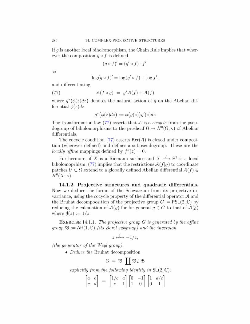
286 14. COMPLEX-PROJECTIVE STRUCTURES
If g is another local biholomorphism, the Chain Rule implies that wher-ever the composition g f is defined,
(g f)′ = (g′ f) · f ′,so
log(g f)′ = log(g′ f) + log f ′,
and differentiating
(77) A(f g) = g∗A(f) + A(f)
where g∗(φ(z)dz
)denotes the natural action of g on the Abelian dif-
ferential φ(z)dz:
g∗(φ(z)dz
):= φ
(g(z)
)g′(z)dz
The transformation law (77) asserts that A is a cocycle from the pseu-dogroup of biholomorphisms to the presheaf Ω 7→ H0(Ω, κ) of Abeliandifferentials.
The cocycle condition (77) asserts Ker(A) is closed under composi-tion (wherever defined) and defines a subpseudogroup. These are thelocally affine mappings defined by f ′′(z) = 0.
Furthermore, if X is a Riemann surface and Xf−−→ P1 is a local
biholomoprhism, (77) implies that the restrictions A(f |U) to coordinatepatches U ⊂ Ω extend to a globally defined Abelian differential A(f) ∈H0(X;κ).
14.1.2. Projective structures and quadratic differentials.Now we deduce the formn of the Schwarzian from its projective in-varriance, using the cocycle property of the differential operator A andthe Bruhat decompoosition of the projective group G := PSL(2,C) byreducing the calculation of A(g) for for general g ∈ G to that of A(J)where J(z) := 1/z
Exercise 14.1.1. The projective group G is generated by the affinegroup B := Aff(1,C) (its Borel subgroup) and the inversion
zJ7−−→ −1/z,
(the generator of the Weyl group).
• Deduce the Bruhat decomposition
G = B∐
B JB
explicitly from the following identity in SL(2,C):[a bc d
]=
[1/c ac 1
] [0 −11 0
] [1 d/c0 1
]

14.1. SCHWARZIAN PAAMETRIZATION 287
when c 6= 0 and ad− bc = 1.• Show that
A(J) =−2
zdz
• Suppose
g(z) =az + b
cz + d.
Then
A(g) =−2
z + d/cdz
• Define a differential operator:
H0(Ω, κ)D−−→ H0(Ω, κ2)
φ(z)dz 7−→ φ′(z)dz2
Show that
(78) DA(g)− 1
2A(g)2 = 0
The formula (78) is reminiscent of the expression of the curvature of aconnection in terms of a connection 1-form and the Fundamental Theo-rem of Calculus for Lie group-valued differential forms (Sharpe [198]).
Now define the Schwarzian differential
Bihol(Ω,P1)S−−→ H0(Ω, κ2)
g 7−→ DA(g)− 1
2A(g)2 =
(g′′g′
)′− 1
2
(g′′g′
)2dz2
where Bihol(Ω,P1) denotes the space of holomorphic maps Ω −→ P1
which are local biholomorphisms, that is meromorphic functions g on Ωfor which g′(z) 6= 0 everywhere on Ω. (The usual Schwarzian derivative,denoted classically by g, z, is the coefficient
(g′′g′
)′− 1
2
(g′′g′
)2
=(g′′′g′
)′− 3
2
(g′′g′
)2
of the Schwarzian derivative S(g).)
Exercise 14.1.2. Prove the cocycle proprty (75).
Although (75) follows from a slightly messy but straihgtforward calcu-lation (see Gunning [109] for example), a more conceptual treatmentis discussed in Hubbard [121]. If g ∈ Bihol(Ω,P1) is a local biholo-morphism, and z0 ∈ Ω, denote the element of G which agrees withg ∈ G to second order at z0 by O(g)z0 ∈ G, the osculating Mobiustransformation for g at z0.

288 14. COMPLEX-PROJECTIVE STRUCTURES
Explicitly, write
g(z) = a0 + a1(z − z0) +a2
2(z − z0)2 +
a3
6(z − z0)3
+ · · ·+ ann!
(z − z0)n + . . .
with a0 = g(z0), a1 = g′(z0) 6= 0, a2 = g′′(z0) and a3 = g′′′(z0). TheMobius transformation
zO(g)z07−−−−−→ a1z
1 + (a2/a1)z
osculates g at z0 and
f(z) = O(g)z0(z) +
(a3
6− a2
2
4a1
)z3 + . . .
The leading term equals 1/a1 times the coefficient of S(g) at z0, that is,the Schwarzian derivative of g at z0. From this conceptual descriptionof S(g) follows the cocycle property (75).
14.1.3. Solving the Schwarzian equation. To show that P(X)is an H0(X, κ2)-torsor, one must show that for any holomorphic qua-dratic differntial Φ = φ(z)dz2, a meromorphic function f ∈ Bihol(X,P1)exists with S(f) = Φ. Furthermore f is unique up to a Mobius trans-formation. That is, given φ, find f solving the nonlinear third orderdifferential equation
(79)
(f ′′
f ′
)′− 1
2
(f ′′
f ′
)2
= φ.
The solution involves relating this nonlinear equation to the secondorder linear differential equation
(80) u′′(z) +1
2φ(z)u(z) = 0
often called Hill’s equation or a Sturm-Liouville equation.
Exercise 14.1.3. Define the projective solution Xf−−→ P1 of (80)
as follows. Every x ∈ X has a neighborhood Ω such that the solutionsof the linear equation (80) on Ω is a a 2-dimensional (complex) vectorspace. Choose a basis u1(z), u2(z) of this vector space and define
Ωf−−→ P1
z 7−→ u1(z)/u2(z)

14.2. FUCHSIAN HOLONOMY 289
• Define the monodromy representation
π1(X) −→ GL(2,C)
of (80) by analytically continuing the local solutions u1, u2 overloops in X.• f is well-defined up to composition with a projective automoor-
phism P1 → P1.• The derivative f ′(z) 6= 0 for all z ∈ Ω.• S(f) = φ(z)dz2.• The projective solution f on Ω analytically continues to a local
biholomorphism
Xf−−→ P1
equivariant with respect to the projectivization π1(X) −→ PGL(2,C)of the monodromy representation of (80).
14.2. Fuchsian holonomy
A related idea is the classification of projective structures withFuchsian holonomy [93]. This is the converse to the grafting con-struction, whereby grafting is the only construction yielding geometricstructures with the same holonomy. Recall that a Fuchsian representa-tion of a surface group π is an embedding of π as a discrete subgroup ofthe group PGL(2,R) ∼= Isom(H2). Equvalently, ρ is the holonomy rep-resentation of a hyperbolic structure on a surface Σ with π1(Σ) ∼= π.The main result is:
Theorem 14.2.1 (Grafting Theorem). Let M be a closed CP1-
manifold whose holonomy representation π1(M)ρ−−→ PSL(2,C) is a
composition
π1(M)ρ0−−→ PGL(2,R) → PSL(2,C)
where ρ0 is Fuchsian representation. Let M0 be a hyperbolic structurewith holonomy representation ρ0, regarded as a CP1-manifold. Thenthere is a unique multicurve S ⊂M0 such that M is obtained from M0
by grafting along S.
However the proof contained a gap, which I first learned from M.Kapovich, who pointed me to the paper of Kuiper [152]. (The same gapcan be found in papers of Goldman-Kamishima [88] and Faltings [76].)This gap was later filled by Choi-Lee [59]. Here we give a correct proof,based on Kulkarni-Pinkall [156] (Theorem 4.2), communicated to meby Daniele Alessandrini. See also Dupont [70].
The grafting theorem uses the setup of Exercise 5.2.8, which webriefly recall. Let M be a connected smooth manifold with a universal

290 14. COMPLEX-PROJECTIVE STRUCTURES
covering space MΠ−−→ M with covering group π = π1(M). Give M a
(G,X)-structure and let (dev, ρ) be a developing pair:
• M dev−−−→ X denotes the developing map;
• π ρ−−− Γ < G denotes the holonomy representation.
Suppose that Ω ⊂ X is a Γ-invariant open subset and
MΩ := Π(dev−1Ω) ⊂M
the subdomain of M corresponding to Ω as in Exercise 5.2.8.The author is grateful to Daniele Alessandrini for patiently explain-
ing the details of the following basic result. Recall from §2.6.4 that thenormality domain Nor(Γ, X) consists of points having open neighbor-hoods U such that
Γ|U := γ|U | g ∈ Γ ⊂⊂ Map(U,X).
Theorem 14.2.2 (Kulkarni-Pinkall [156], Theorem 4.2). Let Mbe a closed (G,X)-manifold with holonomy group Γ < G. Let Ω ⊂Nor(Γ, X) be a Γ-invariant subset of the normality domain, and MΩ ⊂M the corresponding region of M . Then for each component W ⊂MΩ,
and each component W of Π−1(W ), the restriction
Wdev|
W−−−−→ Ω
is a covering space. In particular dev|W is onto.
The proof of Theorem 14.2.2 breaks into a sequence of lemmas. Weshow that dev|W satisfies the path-lifting criterion for covering spaces:
every path in Ω lifts to a path in W . Specifically, let
[0, 1]γ−−→ Ω
be a path in Ω and consider a point
w0 ∈ Π−1(γ(0)
)∩ W
We seek a path
[0, 1]c−→ W
satisfying:
• c(0) = w0;• dev c = γ.
Since dev is a local homeomorphism, the set T of t ∈ [0, 1] such that
[0, t]γ|[0,t]−−−−→ Ω lifts to
[0, t]c|[0,t]−−−−→ W

14.2. FUCHSIAN HOLONOMY 291
is open. Since dev is a local homeomorphism, any extension c|[0,t] ofthe lift to [0, t] is necessarily unique. Thus T is a connected openneighborhood of 0 in [0, 1]. By reparametrizing c, we may assume thatc is defined on [0, 1). It suffices to show that c lifts to [0, 1].
Let c = Π c be the curve in M . Since M is compact and
[0, 1)c−→ Π(W ) ⊂M,
the curve c accumulates in M . That is, a sequence tn ∈ [0, 1) withtn 1 and z ∈M exists, such that
limn→∞
c(tn) = z.
Employ z as the basepoint in M . Fix the corresponding universal
covering space MΠ−−→ M , where M comprises relative homotopy of
paths γ in M starting at z. Recall that the deck transformation of Mcorresponding to the relative homotopy class [β] ∈ π1(M, z) of a loopβ based at z is:
[γ] 7−→ [γ ? β].
Choose a developing map Mdev−−−→ X. Relate to 11.4.
Let U 3 z be an evenly covered coordinate patch in M such thatthe restriction of dev to some (and hence every) component of Π−1(U)is a homeomorphism. Passing to a subsequence if necessary, we mayassume that c(tn) ∈ U for all n. Choose paths z
αn c(tn) in U . Thenthe concatenation
α1 ? c|[t1,tn] ? α−1n
is a based loop βn in M having relative homotopy class [βn] ∈ π1(M, z).
Let U be the component of Π−1(U) containing c(t1), and z the unique
element of U ∩Π−1(z). To simplify notation, denote the deck transfor-mation [βn] by βn.
Lemma 14.2.3.
limn−→∞
ρ(βn)−1γ(tn) = dev(z).
Proof. For n 1, each c(tn) ∈ U . The definition of the deck
transformation βn implies that c(tn) ∈ βnU . Hence
β−1n c(tn) ∈ U .

292 14. COMPLEX-PROJECTIVE STRUCTURES
Since c(tn) −→ z and Π|U is bijective, limn→∞ β−1n c(tn) = z. Continuity
of dev implies:
limn→∞
ρ(β−1n )γ(tn) = lim
n→∞ρ(β−1
n )dev(c(tn)) = limn→∞
dev(β−1n c(tn)
)
= dev(
limn→∞
β−1n c(tn)
)= dev(z),
as claimed.
Conclusion of the proof of Theorem 14.2.2. Apply the con-dition of normality to the images
ρ(βn)−1 γof the curve [0, 1]
γ−−→ Ω. By the definition of Ω, each γ(s) has an openneighborhood Us for which the set of restrictions ρ(βn)|Us is precompactin Map(Us, X). Compactness of [0, 1] guarantees finitely many si existso that the Usi cover [0, 1]. It follows that the images ρ(βn)−1γ form aprecompact sequence in Map
([0, 1], X
). After passing to a subsequence,
we may assume that ρ(βn)−1 γ converges uniformly to a continuous
map [0, 1]δ−→ X.
Now apply Lemma 14.2.3, using the uniform convergence
ρ(βn)−1 γ ⇒ δ,
obtaining
limt→1
dev(c(t))
= δ(1) ∈ dev(U).
Since dev|U is injective, defining
c(1) :=(dev|βN U
)−1(δ(1)
)
is the desired continuous extension of c. The proof of Theorem 14.2.2is complete.
14.3. Thurston parametrization
We briefly summarize some of the unpublished work of Thurston(but see Kamishima-Tan [131] andd Dumas [69]). Then we discuss itsextension by Kulkarni and Pinkall [156, 157]; see also Matsumoto [171].)
14.4. Higher dimensions: flat conformal and sphericalCR-structures
These structures generalize to (G,X)-structures whereG is a semisim-ple Lie group and X = G/P , where P ⊂ G is a parabolic subgroup.The simplest generalization occurs when G = SO(n+1, 1) and X = Sn.The conformal automorphisms of Sn are just Mobius transformations.

14.4. HIGHER DIMENSIONS 293
In this case X is the model space for conformal (Euclidean) geometryand a (G,X)-structure is a flat conformal structure, that is, a conformalequivalence class of conformally flat Riemannian metrics.
A key point in this identification is the famous result of Liouville,that, in dimensions > 2, a conformal map from a nonempty connecteddomain in Sn is the restriction of a unique Mobius transformation ofSn.
Furthermore this is the boundary structure for hyperbolic struc-tures in dimension n+1, since Sn = ∂Hn+1
R and the group of isometriesof Hn+1 restricts to the group of conformal automorphisms of Sn.
The boundary structure for complex hyperbolic geometry is a spher-ical CR-structure, where G = PU(n, 1) and X = ∂Hn
C ≈ S2n−1.For more information on this very active field of research see the
papers of Parker, Falbel, Schwartz, Gusevskii, Deraux, Paupert, Will. Complete!


CHAPTER 15
Geometric structures on 3-manifolds
In this final chapter we collect a few results on Ehresmann struc-tures on closed 3-manifolds. Of course, the relationship with Thurstongeometrization is crucial, since the Thurston geometric structures pro-vide a convenient starting point for understanding the more exoticEhresmann structures. However, the theory is very much in its in-fancy and certain innocent-sounding questions seem (at least now) tobe inaccessible.
The exception is the theory of complete affine structures on 3-manifolds. The classification of such structures on closed 3-manifoldshas been understood since the early 1980’s, see Fried-Goldman [94, 85].The considerably more interesting case of noncompact complete 3-manifolds has only been understood recently. The big breakthroughcame in the early 1980’s with Margulis’s resolution [167] of Milnor’squestion [178]; see Abels [1] and Goldman [98, 99] for expositions.
For possibly incomplete structures, much less is known. We thendescribe a few cases where one has definitive information, includingthe case of closed affine 3-manifolds with nilpotent holonomy and thebeautiful classification of Serge Dupont [71] of affine structures on hy-perbolic torus bundles.
Finally we discuss a few results concerning geometric structures onclosed 3-manifolds, in particular RP3-structures, flat conformal struc-tures, and spherical CR-structures.
15.1. Complete affine structures on 3-manifolds
Complete affine structures on 3-manifolds were classified by Fried-Goldman [85]. They are finitely covered by complete affine solvman-ifolds (see §8.6.2 of Chapter 8) and thus relate to left-invariant affinestructures on 3-dimensional Lie groups (see Chapter 10).
15.1.1. Complete affine 3-manifolds. The first step in the clas-sification is the Milnor-Auslander question: Namely, if M3 = A3/Γ,show that Γ is solvable. Let A(Γ) denote the Zariski closure of Γ inAff(A3; clearly it suffices to show that A(Γ) is solvable. This is equiva-lent to showing that the Zariski closure A(L(Γ)) in GL(R3) of the linear
295

296 15. GEOMETRIC STRUCTURES ON 3-MANIFOLDS
holonomy group L(Γ) ⊂ GL(R3) is solvable. The proof is a case-by-caseanalysis of the possible Levi factors of A(L(Γ)).
The structures on Euclidean 3-manifolds are classified using 3-dimensionalcommutative associative algebras; see Chapter 10, Exercise 10.5.3.
15.1.2. Complete affine structures on noncompact 3-manifolds.In his 1977 paper [178], Milnor set the record straight caused by theconfusion surrounding Auslander’s flawed proof of Conjecture 8.6.2.Influenced by Tits’s work and amenability, Milnor observed, that foran affine space A of given dimension, the following conditions are allequivalent:
• Every discrete subgroup of Aff(A) which acts properly on A isamenable.• Every discrete subgroup of Aff(A) which acts properly on A is
virtually solvable.• Every discrete subgroup of Aff(A) which acts properly on A is
virtually polycyclic.• A nonabelian free subgroup of Aff(A) cannot act properly on
A.• The Euler characteristic χ(Γ\A) (when defined) of a complete
affine manifold Γ\A must vanish (unless Γ = 1 of course).• A complete affine manifold Γ\A has finitely generated funda-
mental group Γ.
(If these conditions were met, one would have a satisfying structuretheory, similar to, but somewhat more involved, than the Bieberbachstructure theory for flat Riemannian manifolds.)
In for this “conjecture”. For example, the infinitesimal version:Namely, let G ⊂ Aff(A) be a connected Lie group which acts prop-erly on A. Then G must be an amenable Lie group, which simplymeans that it is a compact extension of a solvable Lie group. (Equiv-alently, its Levi subgroup is compact.) Furthermore, he provides aconverse: Milnor shows that every virtually polycyclic group admits aproper affine action. (However, Milnor’s actions do not have compactquotient. Benoist [19, 21] found finitely generated nilpotent groupswhich admit no affine crystallographic action. Benoist’s examples are11-dimensional.)
However convincing as his “evidence” is, Milnor still proposes apossible way of constructing counterexamples:
“Start with a free discrete subgroup of O(2, 1) andadd translation components to obtain a group of affinetransformations which acts freely. However it seems

15.2. MARGULIS SPACETIMES 297
difficult to decide whether the resulting group actionis properly discontinuous.”
This is clearly a geometric problem: As Schottky showed in 1907, freegroups act properly by isometries on hyperbolic 3-space, and hence bydiffeomorphisms of A3. These actions are not affine.
One might try to construct a proper affine action of a free group bya construction like Schottky’s. Recall that a Schottky group of rank gis defined by a system of g open half-spaces H1, . . . , Hg and isometriesA1, . . . , Ag such that the 2g half-spaces
H1, . . . , Hg, A1(Hc1), . . . Ag(H
cg)
are all disjoint (where Hc denotes the complement of the closure H ofH). The slab
Slabi := Hci ∩ Ai(Hi)
is a fundamental domain for the action of the cyclic group 〈Ai〉. Theping-pong lemma then asserts that the intersection of all the slabs
∆ := Slab1 ∩ · · · ∩ Slabg
is a fundamental domain for the group Γ := 〈A1, . . . , Ag〉. FurthermoreΓ is freely generated by A1, . . . , Ag. The basic idea is the following. LetB+i := Ai(H
ci ) (respectively B−i := Hi) denote the attracting basin for
Ai (respectively A−1i ). That is, Ai maps all of Hc
i to B+i and A−1
i mapsall of Ai(Hi) to B−i . Let w(a1, . . . , ag) be a reduced word in abstractgenerators a1, . . . , ag, with initial letter a±i . Then
w(A1, . . . , Ag)(∆) ⊂ B±i .
Since all the basins B±i are disjoint, w(A1, . . . , Ag) maps ∆ off itself.Therefore w(A1, . . . , Ag) 6= 1.
Freely acting discrete cyclic groups of affine transformations havefundamental domains which are parallel slabs, that is, regions boundedby two parallel affine hyperplanes. One might try to combine suchslabs to form “affine Schottky groups”, but immediately one sees thisidea is doomed, if one uses parallel slabs for Schottky’s construction:parallel slabs have disjoint complements only if they are parallel toeach other, in which case the group is necessarily cyclic anyway. Fromthis viewpoint, a discrete group of affine transformations seems veryunlikely to act properly.
15.2. Margulis spacetimes
In the early 1980’s Margulis, while trying to prove that a nonabelianfree group can’t act properly by affine transformations, discovered thatdiscrete free groups of affine transformations can indeed act properly!

298 15. GEOMETRIC STRUCTURES ON 3-MANIFOLDS
Around the same time, David Fried and I were also working on thesequestions, and reduced Milnor’s question in dimension three to whatseemed at the time to be one annoying case which we could not handle.Namely, we showed the following: Let A be a three-dimensional affinespace and Γ ⊂ Aff(A). Suppose that Γ acts properly on A. Then eitherΓ is polycyclic or the restriction of the linear holonomy homomorphism
ΓL−→ GL(A)
discretely embeds Γ onto a subgroup of GL(A) conjugate to the orthog-onal group O(2, 1).
In particular the complete affine manifold M3 = Γ\A is a completeflat Lorentz 3-manifold after one passes to a finite-index torsion-freesubgroup of Γ to ensure that Γ acts freely. In particular the restrictionL|Γ defines a free properly discrete isometric action of Γ on the hyper-bolic plane H2 and the quotient Σ2 := H2/L(Γ) is a complete hyperbolicsurface with a homotopy equivalence
M3 := Γ\A ' H2/L(Γ) =: Σ2.
Already this excludes the case when M3 is compact, since Γ is thefundamental group of a closed aspherical 3-manifold (and has cohomo-logical dimension 3) and the fundamental group of a hyperbolic surface(and has cohomological dimension ≤ 2). This is a crucial step in theproof of Conjecture 8.6.2 in dimension 3.
That the hyperbolic surface Σ2 is noncompact is a much deeperresult due to Geoffrey Mess Later proofs and a generalization have beenfound by Goldman-Margulis (Compare the discussion in §15.2.3.) Sincethe fundamental group of a noncompact surface is free, Γ is a free group.Furthermore L|Γ embeds Γ as a free discrete group of isometries ofhyperbolic space. Thus Milnor’s suggestion is the only way to constructnonsolvable examples in dimension three.
15.2.1. Affine boosts and crooked planes. Since L embeds Γ0
as the fundamental group of a hyperbolic surface, L(γ) is elliptic onlyif γ = 1. Thus, if γ 6= 1, then L(γ) is either hyperbolic or parabolic.Furthermore L(γ) is hyperbolic for most γ ∈ Γ0.
When L(γ) is hyperbolic, γ is an affine boost, that is, it has theform
(81) γ =
e`(γ) 0 0
0 1 00 0 e−`(γ)
0α(γ)
0
in a suitable coordinate system. (Here the 3× 3 matrix represents thelinear part, and the column 3-vector represents the translational part.)

15.2. MARGULIS SPACETIMES 299
γ leaves invariant a unique (spacelike) line Cγ (the second coordinateline in (81). Its image in E2,1/Γ is a closed geodesic Cγ/〈γ〉. Just asfor hyperbolic surfaces, most loops in M3 are freely homotopic to suchclosed geodesics. (For a more direct relationship between the dynamicsof the geodesic flows on Σ2 and M3, compare Goldman-Labourie
Margulis observed that Cγ inherits a natural orientation and metric,arising from an orientation on A, as follows. Choose repelling andattracting eigenvectors L(γ)± for L(γ) respectively; choose them so theylie in the same component of the nullcone. Then the orientation andmetric on Cγ is determined by a choice of nonzero vector L(γ)0 spanningFix(L(γ)
). this vector is uniquely specified by requiring that:
• L(γ)0 · L(γ)0 = 1;•(L(γ)0, L(γ)−, L(γ)+
)is a positively oriented basis.
The restriction of γ to Cγ is a translation by displacement α(γ) withrespect to this natural orientation and metric.
Compare this to the more familiar geodesic length function `(γ)associated to a class γ of closed curves on the hyperbolic surface Σ.The linear part L(γ) acts by transvection along a geodesic cL(γ) ⊂ H2.The quantity `(γ) > 0 measures how far L(γ) moves points of cL(γ).
This pair of quantities(`(γ), α(γ)
)∈ R+ × R
is a complete invariant of the isometry type of the flat Lorentz cylinderA/〈γ〉. The absolute value |α(γ)| is the length of the unique primitiveclosed geodesic in A/〈γ〉.
A fundamental domain is the parallel slab
(ΠCγ )−1(p0 + [0, α(γ)] γ0
)
where
AΠCγ−−→ Cγ
denotes orthogonal projection onto
Cγ = p0 + Rγ0.
As noted above, however, parallel slabs can’t be combined to formfundamental domains for Schottky groups, since their complementaryhalf-spaces are rarely disjoint.
In retrospect this is believable, since these fundamental domainsare fashioned from the dynamics of the translational part (using theprojection ΠCγ ). While the effect of the translational part is properness,the dynamical behavior affecting most points is influenced by the linearpart: While points on Cγ are displaced by γ at a polynomial rate, allother points move at an exponential rate.

300 15. GEOMETRIC STRUCTURES ON 3-MANIFOLDS
Furthermore, parallel slabs are less robust than slabs in H2: whilesmall perturbations of one boundary component extend to fundamentaldomains, this is no longer true for parallel slabs. Thus one mightlook for other types of fundamental domains better adapted to theexponential growth dynamics given by the linear holonomy L(γ).
Todd Drumm, in his 1990 Maryland thesis defined more flexiblepolyhedral surfaces, which can be combined to form fundamental do-mains for Schottky groups of 3-dimensional affine transformations. Acrooked plane is a PL surface in A, separating A into two crooked half-spaces. The complement of two disjoint crooked halfspace is a crookedslab, which forms a fundamental domain for a cyclic group generatedby an affine boost. Drumm proved the remarkable theorem that ifS1, . . . , Sg are crooked slabs whose complements have disjoint interiors,then given any collection of affine boosts γi with Si as fundamental do-main, then the intersection S1 ∩ · · · ∩ Sg is a fundamental domain for〈γ1, . . . , γg〉 acting on all of A.
Modeling a crooked fundamental domain for Γ acting on A on afundamental polygon for Γ0 acting on H2, Drumm proved the followingsharp result:
Theorem (Drumm ). Every noncocompact torsion-free Fuchsiangroup Γ0 admits a proper affine deformation Γ whose quotient is a solidhandlebody.
15.2.2. Marked length spectra. We now combine the geodesiclength function `(γ) describing the geometry of the hyperbolic surfaceΣ with the Margulis invariant α(γ) describing the Lorentzian geometryof the flat affine 3-manifold M .
As noted by Margulis, α(γ) = α(γ−1), and more generally
α(γn) = |n|α(γ).
The invariant ` satisfies the same homogeneity condition, and therefore
α(γn)
`(γn)=
α(γ)
`(γ)
is constant along hyperbolic cyclic subgroups. Hyperbolic cyclic sub-groups correspond to periodic orbits of the geodesic flow φ on the unittangent bundle UΣ. Periodic orbits, in turn, define φ-invariant prob-ability measures on UΣ. Goldman-Labourie-Margulis prove that, forany affine deformation, this function extends to a continuous functionΥΓ on the space C(Σ) of φ-invariant probability measures on UΣ. Fur-thermore when Γ0 is convex cocompact (that is, contains no parabolicelements), then the affine deformation Γ acts properly if and only if ΥΓ

15.2. MARGULIS SPACETIMES 301
never vanishes. Since C(Σ) is connected, nonvanishing implies eitherall ΥΓ(µ) > 0 or all ΥΓ(µ) < 0. From this follows Margulis’s OppositeSign Lemma, first proved in to groups with parabolics by Charette andDrumm
Theorem (Margulis). If Γ acts properly, then all of the numbersα(γ) have the same sign.
For an excellent treatment of the original proof of this fact, see thesurvey article of Abels
15.2.3. Deformations of hyperbolic surfaces. The Margulisinvariant may be interpreted in terms of deformations of hyperbolicstructures as follows
Suppose Γ0 is a Fuchsian group with quotient hyperbolic surfaceΣ0 = Γ0\H2. Let gAd be the Γ0-module defined by the adjoint rep-resentation applied to the embedding Γ0 → O(2, 1). The coefficientmodule gAd corresponds to the Lie algebra of right-invariant vectorfields on O(2, 1) with the action of O(2, 1) by left-multiplication. Geo-metrically these vector fields correspond to the infinitesimal isometriesof H2.
A family of hyperbolic surfaces Σt smoothly varying with respectto a parameter t determines an infinitesimal deformation, which is acohomology class [u] ∈ H1(Γ0, gAd), The cohomology group H1(Γ0, gAd)corresponds to infinitesimal deformations of the hyperbolic surface Σ0.In particular the tangent vector to the path Σt of marked hyperbolicstructures smoothly varying with respect to a parameter t defines acohomology class
[u] ∈ H1(Γ0, gAd).
The same cohomology group parametrizes affine deformations. Thetranslational part u of a linear representations of Γ0 is a cocycle of thegroup Γ0 taking values in the corresponding Γ0-module V. Moreovertwo cocycles define affine deformations which are conjugate by a trans-lation if and only if their translational parts are cohomologous cocycles.Therefore translational conjugacy classes of affine deformations formthe cohomology group H1(Γ0,V). Inside H1(Γ0,V) is the subset Propercorresponding to proper affine deformations.
The adjoint representation Ad of O(2, 1) identifies with the orthog-onal representation of O(2, 1) on V. Therefore the cohomology groupH1(Γ0,V) consisting of translational conjugacy classes of affine defor-mations of Γ0 can be identified with the cohomology group H1(Γ0, gAd)corresponding to infinitesimal deformations of Σ0.

302 15. GEOMETRIC STRUCTURES ON 3-MANIFOLDS
Theorem. Suppose u ∈ Z1(Γ0, gAd) defines an infinitesimal defor-mation tangent to a smooth deformation Σt of Σ.
• The marked length spectrum `t of Σt varies smoothly with t.• Margulis’s invariant αu(γ) represents the derivative
d
dt
∣∣∣∣t=0
`t(γ)
• (Opposite Sign Lemma) If [u] ∈ Proper, then all closed geodesicslengthen (or shorten) under the deformation Σt.
Since closed hyperbolic surfaces do not support deformations in whichevery closed geodesic shortens, such deformations only exist when Σ0
is noncompact. This leads to a new proof [105] of Mess’s theoremthat Σ0 is not compact. (For another, somewhat similar proof, whichgeneralizes to higher dimensions, see Labourie [158].)
The tangent bundle TG of any Lie group G has a natural structure
as a Lie group, where the fibration TGΠ−→ G is a homomorphism of Lie
groups, and the tangent spaces
TxG = Π−1(x) ⊂ TG
are vector groups. The deformations of a representation Γ0ρ0−→ G
correspond to representations Γ0ρ−→ TG such that Π ρ = ρ0. In our
case, affine deformations of Γ0 → O(2, 1) correspond to representationsin the tangent bundle TO(2, 1). When G is the group G(R) of R-pointsof an algebraic group G defined over R, then
TG ∼= G(R[ε])
where ε is an indeterminate with ε2 = 0. (Compare [97].) This isreminiscent of the classical theory of quasi-Fuchsian deformations ofFuchsian groups, where one deforms a Fuchsian subgroup of SL(2,R)in
SL(2,C) = SL(2,R[i])
where i2 = −1.
15.2.4. Classification. In light of Drumm’s theorem, classifyingMargulis spacetimes M3 begins with the classification of hyperbolicstructures Σ2. Thus the deformation space of Margulis spacetimesmaps to the Fricke space F(Σ) of marked hyperbolic structures on theunderlying topology of Σ.
The main result of is that the positivity (or negativity) of ΥΓ on onC(Σ) is necessary and sufficient for properness of Γ. (For simplicity werestrict ourselves to the case when L(Γ) contains no parabolics — thatis, when Γ0 is convex cocompact.) Thus the proper affine deformation

15.2. MARGULIS SPACETIMES 303
space Proper identifies with the open convex cone in H1(Γ0,V) definedby the linear functionals Υµ, for µ in the compact space C(Σ). Thesegive uncountably many linear conditions on H1(Γ0,V), one for each µ ∈C(Σ). Since the invariant probability measures arising from periodicorbits are dense in C(Σ), the cone Proper is the interior of half-spacesdefined by the countable set of functional Υγ, where γ ∈ Γ0.
The zero level sets Υ−1γ (0) correspond to affine deformations where
γ does not act freely. Therefore Proper defines a component of thesubset of H1(Γ0,V) corresponding to affine deformations which are freeactions.
Actually, one may go further. An argument inspired by Thurston thosemeasures arising from multicurves, that is, unions of disjoint simpleclosed curves. These measures (after scaling) are dense in the Thurstoncone ML(Σ) of measured geodesic laminations on Σ. One sees the com-binatorial structure of the Thurston cone replicated on the boundaryof Proper ⊂ H1(Γ0,V).
Two particular cases are notable. When Σ is a 3-holed sphere ora 2-holed cross-surface (real projective plane), then the Thurston conedegenerates to a finite-sided polyhedral cone. In particular propernessis characterized by 3 Margulis functionals for the 3-holed sphere, and 4for the 2-holed cross-surface. Thus the deformation space of equivalenceclasses of proper affine deformations is either a cone on a triangle or aconvex quadrilateral, respectively.
When Σ is a 3-holed sphere, these functionals correspond to thethree components of ∂Σ. The halfspaces defined by the correpondingthree Margulis functionals cut off the deformation space (which is apolyhedral cone with 3 faces). The Margulis functionals for the othercurves define halfspaces which strictly contain this cone.
When Σ is a 2-holed cross-surface these functionals correspond tothe two components of ∂Σ and the two orientation-reversing simpleclosed curves in the interior of Σ. The four Margulis functionals de-scribe a polyhedral cone with 4 faces. All other closed curves on Σdefine halfspace strictly containing this cone.
In both cases, an ideal triangulation for Σ models a crooked funda-mental domain for M , and Γ is an affine Schottky group, and M is anopen solid handlebody of genus 2 (Charette-Drumm-Goldman depictsthese finite-sided deformation spaces.
For the other surfaces where π1(Σ) is free of rank two (equivalentlyχ(Σ) = −1), infinitely many functionals Υµ are needed to define thedeformation space, which necessarily has infinitely many sides. In thesecases M3 admits crooked fundamental domains corresponding to idealtriangulations of Σ, although unlike the preceding cases there is no

304 15. GEOMETRIC STRUCTURES ON 3-MANIFOLDS
single ideal triangulation which works for all proper affine deformations.Once again M3 is a genus two handlebody.
15.3. Dupont’s classification of hyperbolic torus bundles
This builds on Dupont’s classification of affine actions of the two-dimensional group Aff(R) on A3, see Dupont [70].
15.3.1. Hyperbolic torus bundles. Although the class of affinestructures on closed 3-manifolds with nilpotent holonomy are under-stood, the general case of solvable holonomy remains mysterious. How-ever, Serge Dupont [71] completely classifies affine structures on 3-manifolds with solvable fundamental group. (Compare also Dupont [70],in the volume [123].) In terms of the Thurston geometrization, theseare the geometric 3-manifolds modeled on Sol, that is, 3-manifoldsfinitely covered by hyperbolic torus bundles: mapping tori (suspen-sions) of hyperbolic elements of GL(2,Z). Dupont shows that all suchstructures arise from left-invariant affine structures on the correspond-ing Lie group G, which is the semidirect product of R2 by R, where Racts on R2 as a unimodular hyperbolic one-parameter subgroup (explic-itly, G is isomorphic to the identity component in the group of Lorentzisometries of the Minkowski plane).
Two structures are particularly interesting for the behavior of geo-desics in light of the results of Vey [222]. A properly convex domainΩ ∈ An is said to be divisible if Ω admits a discrete group Γ of pro-jective automorphisms acting properly on Ω such that Ω/Γ is com-pact. (Equivalently, the quotient space Ω/Γ by a discrete subgroupΓ ⊂ Aut(Ω) is compact and Hausdorff.) Vey proved that a divisibledomain is a cone. However, dropping the properness of the action of Γon Ω allows counterexamples: the parabolic cylinder
Ω := (x, y) ∈ A2 | y > x2is a properly convex domain which is not a cone, but admits a groupΓ of automorphisms such that Ω/Γ is compact but not Hausdorff.This group needs
a succinct name. Now take the product Ω×R ⊂ A3. Let G < Aff(A3) be the subgroupacting simply transitively (isomorphic to the 3-dimensional unimodularexponential non-nilpotent solvable Lie group) discussed in §10.8.1), andlet Γ < G be a lattice. Then Γ acts properly on Ω× R and:
• The quotient M = (Ω × R)/Γ is a hyperbolic torus bundle(and in particular compact and Hausdorff);• Ω× R is not a cone.
Clearly Ω×R is not properly convex, showing that Vey’s result is sharp.(Compare Goldman [91].)

15.4. EXAMPLES OF PROJECTIVE THREE-MANIFOLDS 305
The Kobayashi pseudometric degenerates along a 1-dimensional fo-liation of M , and defines the hyperbolic structure transverse to thisfoliation discussed by Thurston [211], Chapter 4.
15.4. Examples of projective three-manifolds


APPENDIX A
Transformation groups
A.1. Group actions
We shall consider left-actions of a group on a set, unless otherwisenoted. Suppose that G is a group acting on a set X, with the (left-)action denoted by:
G×X α−−→ X
(g, x) 7−→ g · xWe refer to X as a (left-) G-set.
The kernel of the action α consists of all g such that α(g, ·) = I,that is, g · x = x,∀x ∈ X. Equivalently, this is the kernel of thehomomorphism of G into the group of automorphisms of the set X.The action is effective (or faithful) if its kernel is trivial.
If x ∈ X, its stabiliizer: is the subgroup:
Stab(x) := g ∈ G | g · x = x.If g ∈ G, then its fixed-point set (or stationary set is the subset:
Fix(g) := x ∈ X | g · x = x.The action is free if and only if Stab(x) = 1,∀x ∈ X, or equivalentlyFix(g) = ∅,∀g ∈ G, g 6= 1.
The orbit of a point x is the image
G · x := α(G× x) = g · x | g ∈ G.The orbits partition X, so that the group action defines an equiva-
lence relation on X. The action is transitive if some (and hence every)orbit equals X.
The action is simply transitive if it is transitive and free. In termsof the orbit map (or evaluation map)
Gαx−−→ X
g 7−→ α(g, x) = g · x,• α is free x ⇐⇒ αx is injective ∀x ∈ X;• α is transitive ⇐⇒ αx is injective (for any x);• α is simply transitive ⇐⇒ αx is bijective.
307

308 A. TRANSFORMATION GROUPS
A simply transitive action α makes X into a G-torsor.
Exercise A.1.1. Let X be a left G-set and x ∈ X. Let H =Stab(x).
• The orbit map αx defines a G-equivariant isomorphism G/H −→G · x. where G acts by left-multiplicataion on the set G/H ofleft cosets gH for g ∈ G.• Suppose that N < H is a nontrivial normal subgroup of G.
Then G does not act effectively on G/H.
A.2. Proper and syndetic actions
A convenient context in which to work is that of locally compactHausdorff topologyical spaces and topoological groups. Recall that a
continuous mapXf−−→ Y is proper if ∀K ⊂⊂ Y , the preimage f−1(K) ⊂⊂
X. Recall the following facts from general topology:
• A closed subset of a compact space is compact.• The continuous image of a compact space is compact.• Compact subsets of a Hausdorff space are closed,
It follows that a proper map is closed.
Exercise A.2.1. Suppose that X, Y are manifolds and f is a smoothmap. Furthermore suppose that f is a local homeomoprhism. Then fis a covering space.
Let G be a locally compact Hausdorff topological group and
G×X α−−→ X
(g, x) 7−→ g · xis a (left) action. We say that the group action α is proper if and onlyif the continuous map
G×X fα−−→ X ×X(g, x) 7−→ (g · x, x)
is a proper map.
Exercise A.2.2. Show that properness is equivalent to the eitherof the two following conditions: (for the last condition assume that Gis second countable)
• ∀K1, K2 ⊂⊂ X, the set
G(K1, K2) := g ∈ G | gK1 ∩K2 6= ∅ ⊂⊂ G.
• ∀K ⊂⊂ X, G(K,K) ⊂⊂ G.

A.3. TRANSFORMATION GROUPOIDS 309
• For all sequences gn ∈ G, xn ∈ X, such that gnxn converges,the sequence gn has a convergent subsequence.
For the last condition, we can say that if xn stays bounded, but gn →∞,then gnxn →∞.
Exercise A.2.3. Suppose that α is a proper action of a locally com-pact group on a locally compact Hausdorff space X. Then the quotientspace G\X is Hausdorff. Is the converse true?
Exercise A.2.4. Suppose that Γ is a discrete group and G×X α−−→X is a proper free action. Then the quotient map X −→ G\X is acovering space.
A group action α is syndetic if the quotient G\X is compact.
A.3. Topological transformation groupoids
We must relate the actions of Aff(A) on C(A) and G on C(P). Recallthat a topological transformation groupoid consists of a small categoryG whose objects form a topological space X upon which a topologicalgroup G acts such that the morphisms a→ b consist of all g ∈ G suchthat g(a) = b. We write G = (G,X). A homomorphism of topologicaltransformation groupoids is a functor
(X,G)(f,F )−−−−→ (X ′, G′)
arising from a continuous map Xf−−→ X ′ which is equivariant with
respect to a contin uous homomorphism GF−−→ G′.
The space of isomorphism classes of objects in a category G will bedenoted Iso(G). We shall say that G is proper (respectively syndetic)if the corresponding action of G on X is proper (respectively synde-
tic). If G and G′ are topological categories, a functor GF−−→ G′ is an
equivalence of topological categories if the induced map
Iso(G)Iso(F )−−−−→ Iso(G′)
is a homeomorphism and F is fully faithful, that is, for each pair ofobjects a, b of G, the induced map
Hom(a, b)F∗−−→ Hom(F (a), F (b))
is a homeomorphism. If F is fully faithful it is enough to prove thatIso(F ) is surjective. (Compare Jacobson [124].) We have the followinggeneral proposition:

310 A. TRANSFORMATION GROUPS
Lemma A.3.1. Suppose that
(X,G)(f,F )−−−−→ (X ′, G′)
is a homomorphism of topological transformation groupoids which is anequivalence of groupoids and such that f is an open map.
• If (X,G) is proper, so is (X ′, G′).• If (X,G) is syndetic, so is (X ′, G′).
Proof. An equivalence of topological groupoids induces a homeo-morphism of quotient spaces
X/G −→ X ′/G′
so if X ′/G′ is compact (respectively Hausdorff) so is X/G. Since (X,G)is syndetic if and only if X/G is compact, this proves the assertionabout syndeticity. By Koszul [148], p.3, Remark 2, (X,G) is proper ifand only if X/G is Hausdorff and the action (X,G) is wandering (orlocally proper): each point x ∈ X has a neighborhood U such that
G(U,U) = g ∈ G | g(U) ∩ U 6= ∅is precompact. Since (f, F ) is fully faithful, F maps G(U,U) isomor-phically onto G′(f(U), f(U)). Suppose that (X,G) is proper. ThenX/G is Hausdorff and so is X ′/G′. We claim that G′ acts locallyproperly on X ′. Let x′ ∈ X ′. Then there exists g′ ∈ G′ and x ∈ Xsuch that g′f(x) = x′. Since G acts locally properly on X, there ex-ists a neighborhood U of x ∈ X such that G(U,U) is precompact.It follows that U ′ = g′f(U) is a neighborhood of x′ ∈ X ′ such thatG′(U ′, U ′) ∼= G(U,U) is precompact, as claimed. Thus G′ acts prop-erly on X ′.

APPENDIX B
Affine connections in local coordinates
We summarize some ot the basic facts about (not necessarily flat)affine connections on a smooth manifold M . After discussing the ex-pression of general affine connections in local coordinates is a reviewof the Levi-Civita (or Riemannian) connection. As this general the-ory only uses the nondegeneracy of the metric connection, it appliesequally to pseudo-Riemannian, structures defined by a (possibly indef-inite) metric tensor. Due to its fundamental importance, this appendixends with a detailed discussion of the Riemannian connection for thehyperbolic plane H2.
B.1. Affine connections in local coordinates
Recall that an affine connection on M is a (linear connection) onthe tangent bundle TM , which can be defined in several different ways.One of the most familiar ways is that of a Koszul connection, that is, acovariant differentiation operation on a vector bundle V over M , whichhappens to be isomorphic to the tangent bundle TM . Explicitly weconsider an isomorphism of vector bundles over M :
TMS−−→ V
together with a covariant differentiation operation
TpM × Γ(V) −→ Vp
(Xp, v) 7−→ ∇Xp(v)
which satisfies tensorial conditions
∇fXp(v) = f(p)∇Xp(v), ∇Xp(fv) = Xp(f)v + f(p)∇Xpv
for f ∈ C∞(M).In local coordinates (x1, . . . , xn), the connection is defined by Christof-
fel symbols∇∂i(∂j) := Γkij(x)∂k.
whereby the general covariant derivative of vector fields is:
∇ai∂ibj∂j = ai∂bj∂xi
Γkij(x)∂k.
311

312 B. AFFINE CONNECTIONS
From an affine connection, define the torsion and curvature tensorsas follows.
Exercise B.1.1. Show that the operations on vector fields X, Y ∈Vec(M)
Tor∇(X, Y ) := ∇XY −∇YX
Riem∇(X, Y ) := ∇X∇Y −∇Y∇X −∇[X,Y ]
are tensorial (that is, multilinear over C∞(M)), and define smoothsections of the vector bundles Λ2(TM)⊗TM and Λ2(TM)⊗End(TM),respectively.
In local coordinates on TM , where (x1, . . . , xn) are local coordi-nates on M and (v1, . . . vn) are local coordinates on TpM , the geodesicequations are:
d
dtxk(t) = vk(t)
d
dtvi(t) = −Γkij(x)vi(t)vj(t)
(for k = 1, . . . , n) and Γkij(x) are the Christoffel symbols defined by:
∇∂i(∂j) = Γkij(x)∂k.
In particular the geodesic flow corresponds to the vector field (calledthe geodesic spray):
φΓ := vk∂
∂xk− Γkij(x)vivj
∂
∂vk
on TM . See Kobayashi-Nomizu [144], do Carmo [67] or O’Neill [182]for further details.
That φΓ is vertically homogeneous of degree one: That is, it trans-forms under the one-parameter group of homotheties
(p,v)ht7−−→ (p, esv)
by
(82) (ht)∗(φΓ) = etφΓ
Furthermore its trajectories are the velocity vector fields of the geodesicson M . Namely, let p = (x1, . . . , xn) ∈ M and v = (v1, . . . vn) ∈ TpMbe an initial condition. Let γp,v(t) ∈ TM denote the trajectory of φM ,defined for t in an open interval containing 0 ∈ R, defined by:
∂
∂t
∣∣∣t=0γp,v(t) = v, γp,v(0) = (p,v)

B.2. THE (PSEUDO-) RIEMANNIAN CONNECTION 313
Then the local flow Φt of φΓ on TM satisfies
Φt(p,v) =(γp,v(t), γ′p,v(t)
),
where
γp,v(t) := (Π Φt)(p,v)
and TMΠ−−→ M denoting the bundle projection. The homogeneity
condition (82) implies that
γp,sv(t) = γp,v(st).
We write:
(83) Expp(tv) := γp,v(t)
for t ∈ R sufficiently near 0. Then, whenever s, t are sufficiently near0,
Expp((s+ t)v
)= Expγ(t)
(sP(tv)
)
where, for clarity, we denote γ(t) := Expp(tv) and parallel transport
Πγ(t)p by:
TpMΠ−−→ Tγ(t).
Observe that Π(v) = γ′(t).Compare §8.3 and standard references.
B.2. The (pseudo-) Riemannian connection
The fundamental theorem of Riemannian geometry asserts a pseudo-Riemannian manifold (M, g) admits a unique affine connection ∇ withnatural properties:
• (Orthogonality) ∇g = 0;• (Symmetry) Tor(∇) = 0.
Orthogonality is equivalent to the condition that the parallel transportoperator
TxMPγ−−→ TyM
along a path xγy maps (Tx, gx) isometrically to (Ty, gy). When com-
puted with respect to an orthonormal frame, this implies that theChristoffel symbols satisfy:
Γkij = −Γjik,
that is, the n× n-matrix of 1-forms[Γkijdx
1]
is skew-symmetric.

314 B. AFFINE CONNECTIONS
Exercise B.2.1. The Koszul formula is an remarkable explicit for-mula for the Levi-Civita connection in terms of the metric tensor g andthe Lie bracket on Vec(M). Namely, if X, Y, Z ∈ Vec(M), then
2g(∇XY, Z) = Xg(Y, Z) + Y g(Z,X)− Zg(X, Y )
− g(X, [Y, Z]) + g(Y, [Z,X]) + g(Z, [X, Y ])
defines the unique affine ∇-ortogonal symmetric connection. In localcoordinates (x1, . . . , xn),
Γkij =1
2gkm(∂gjm∂xi
+∂gim∂xj
− ∂gij∂xm
)
B.3. The Levi-Civita connection for the Poincare metric
We denote complex numbers z = x+ yi ∈ C where x, y ∈ R.Let H2 denote the upper half-plane
x+ iy|x, y ∈ R, y > 0
with the Poincare metric:
g =|dz|2y2
We compute the Levi-Civita connection ∇ with respect to several dif-ferent frames.
B.3.1. The usual coordinate system on H2. Let ∂x, ∂y be thecoordinate vector fields, so that:
g(∂x, ∂x) = g(∂y, ∂y) = y−2(84)
g(∂x, ∂y) = g(∂y, ∂x) = 0.(85)
The vector fields
ξ := y∂x
η := y∂y
define an orthonormal frame field. Therefore, for any vector field φ,
φ = g(φ, ξ)ξ + g(φ, η)η
= y2(
g(φ, ∂x)∂x + g(φ, ∂y)∂y
)(86)

B.3. POINCARE METRIC 315
Theorem. In terms of the coordinate frame, the Levi-Civita con-nection is given by:
∇x∂x = y−1∂y(87)
∇x∂y = −y−1∂x(88)
∇y∂x = −y−1∂x(89)
∇y∂y = −y−1∂y(90)
In terms of the orthonormal frame, the Levi-Civita connection is givenby:
∇ξξ = η
∇ξη = −ξ∇ηξ = 0
∇ηη = 0
Proof. Symmetry of ∇ and [∂x, ∂y] = 0 implies:
(91) ∇x∂y = ∇y∂x
which implies the equivalence (88) ⇐⇒ (89).Differentiate (84) with respect to ∂x:
g(∇x∂x, ∂x) = 0(92)
g(∇x∂y, ∂y) = 0.(93)
Combine (93) with (91):
(94) g(∇y∂x, ∂y) = 0
Differentiate (84) with respect to ∂y:
2g(∇y∂x, ∂x
)= 2g
(∇y∂y, ∂y
)= −2y−3,
whence
(95) g(∇y∂x, ∂x
)= −y−3
and
(96) g(∇y∂y, ∂y
)= −y−3..
Now:
g(∇x∂x, ∂y
)= ∂xg(∂x, ∂y)︸ ︷︷ ︸
0 by (85)
−g(∂x,∇x∂y)(97)
= −g(∂x,∇y∂x) by (91)
= −g(∇y∂x, ∂x) = y−3 by (94),
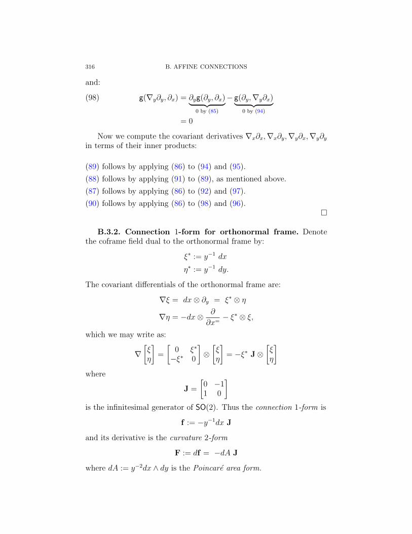
316 B. AFFINE CONNECTIONS
and:
g(∇y∂y, ∂x) = ∂yg(∂y, ∂x)︸ ︷︷ ︸0 by (85)
− g(∂y,∇y∂x)︸ ︷︷ ︸0 by (94)
(98)
= 0
Now we compute the covariant derivatives ∇x∂x,∇x∂y,∇y∂x,∇y∂yin terms of their inner products:
(89) follows by applying (86) to (94) and (95).
(88) follows by applying (91) to (89), as mentioned above.
(87) follows by applying (86) to (92) and (97).
(90) follows by applying (86) to (98) and (96).
B.3.2. Connection 1-form for orthonormal frame. Denotethe coframe field dual to the orthonormal frame by:
ξ∗ := y−1 dx
η∗ := y−1 dy.
The covariant differentials of the orthonormal frame are:
∇ξ = dx⊗ ∂y = ξ∗ ⊗ η
∇η = −dx⊗ ∂
∂x=− ξ∗ ⊗ ξ,
which we may write as:
∇[ξη
]=
[0 ξ∗
−ξ∗ 0
]⊗[ξη
]= −ξ∗ J⊗
[ξη
]
where
J =
[0 −11 0
]
is the infinitesimal generator of SO(2). Thus the connection 1-form is
f := −y−1dx J
and its derivative is the curvature 2-form
F := df = −dA J
where dA := y−2dx ∧ dy is the Poincare area form.

B.3. POINCARE METRIC 317
B.3.3. Geodesic curvature of a hypercycle. We use these tocalculate the geodesic curvature of a hypercycle. The positive imagi-nary axis iR+ is a geodesic with endpoints 0,∞. Let −π/2 < θ < π/2.The ray eiθR+ is a hypercycle hρ at distance ρ ∈ R from the geodesiciR+, where
eiθ = cos(θ) + i sin(θ) = tanh(ρ) + i sech(ρ)
parametrizes the geodesic perpendicular to iR+ through i with unitspeed.
γ(s) := es(
tanh(ρ) + i sech(ρ))
parametrizes hρ with unit speed. Its velocity equals
γ′(s) = es(
tanh(ρ)∂x + sech(ρ)∂y).
Since ‖γ′(s)‖ = 1 the acceleration of γ(the vector D
dsγ′(s)
)is orthogo-
nal to γ and the geodesic curvature of γ equals:
kg =∥∥∥Ddsγ(s)
∥∥∥ = tanh(ρ)
Similarly the geodesic curvature of a metric circle of radius ρ equalscoth(ρ). To see this, use the Poincare unit disc model: for |z| < 1, themetric tensor is:
g :=4|dz|2
(1− |z|2)2
and writing (hyperbolic polar coordinates)
z = eiθ tanh(ρ/2)
the metric tensor is g = dρ2 + sinh2(ρ)dθ2, with area form dA =sinh2(ρ)dρ ∧ dθ. Consider a disc Dρ with (hyperbolic) radius ρ. Thenits circumference equals 2π sinh(ρ) and its area 2π
(cosh(ρ) − 1
). Let
kg be the geodesic curvature of the metric circle ∂Dρ. Applying theGauss-Bonnet theorem
2πχ(Σ) =
∫
Σ
KdA+
∮
∂Σ
kgds
to σ = Dρ obtaining:
2π = −2π(
cosh(ρ)− 1) + kg
(2π sinh(ρ)
),
that is,kg = coth(ρ)
as desired.


APPENDIX C
Facts about metric spaces
This appendix discusses several well-known general facts about met-ric spaces and pseudometric spaces, which are used in §12 and else-where.
C.1. Nonincreasing homeomorphisms are isometries
Here we give the proof of Lemma 4.3.3, which states that a distancenon-increasing homeomorphism of a compact metric space (X, d) isan isometry. This fact is used in the proof of Vey’s Semisimplicity(Theorem 4.3.1.
The proof given here was found on Stack Exchange, submitted byDap on 1 March 2018.
Lemma C.1.1. Suppose (X, d) is a compact metric space and let
Xf−− X be a surjective continuous map such that d
(f(x), f(y)) ≤
d(x, y) for all x, y ∈ X. Then f is an isometry.
Proof. Let ε > 0. Since X is compact, it admits an ε/4-cover,that is, a set S := s1, . . . , sm ⊂ X such that ∀x ∈ X, ∃sj ∈ S withd(sj, x) < ε/4. We may assume that S minimizes the number N(S) ofpairs (si, sj) ∈ S × S with
d(s1, s2) ≥ D := d(x, y)− ε/2.Since f is surjective and distance non-increasing, f(S) is also an ε/4-cover, and d(s1, s2) < D implies d
(f(s1), f(s2)
)< D. Thus
d(f(s1), f(s2)
)≥ D
whenever d(s1, s2) ≥ D and s1, s2 ∈ S.Picking s1, s2 ∈ S with d(s1, x), d(s2, y) ≤ ε/4 gives d(s1, s2) ≥
d(x, y)− ε/2. As above, d(f(s1), f(s2)
)≥ d(x, y)− ε/2, whence
d(f(x), f(y)
)≥ d(x, y)− ε.
319

320 C. METRIC SPACES
C.2. Compactness of distance nonincreasing maps
Recall that a topological space is separable if it has a countabledense subset.
Lemma C.2.1 (Kobayashi [143], Chapter V, Theorem 3.1). Let(N, dN) and (M, dM) be connected locally compact pseudometric spaces.Suppose that (N, dN) is separable and (M, dM) is a complete metricspace. Then the subset of Map(N,M) comprising distance-nonincreasingmaps
Nf−−→M
is locally compact. In particular, if p ∈ N and K ⊂⊂M , the subset ofall such maps with f(p) ∈ K is compact.
We briefly sketch the proof; see Kobayashi [143]for further details.Let fn be a sequence of distance-nonincreasing projective maps tak-
ing p ∈ N to K ⊂⊂ M . Choose a countable dense subset p1, . . . ⊂N ; then
Ki := BdM (K,pi)(K) ⊂⊂M.
Since the fn are distance-nonincreasing,
fn(pi) ∈ Ki.
Passing to a subsequence, assume thatt the sequence fn(pi) converges,for each i. Then for each q ∈ N , the sequence fn(q) is Cauchy. SinceN is complete, fn(q) converges. Finally, this convergence is uniform oncompact subsets of N .
C.3. The Lebesgue number of an open covering
Lemma C.3.1. Let (X, d) be a compact metric space and U an opencovering of X. Then ∃δ > 0 such that every subset Y ⊂ X withdiam(Y ) < δ lies in some U ∈ U .
Proof. Because X is compact, U contains a finite subcoveringU1, . . . , Un. If some Ui = X, then any δ > 0 suffices. Therefore weassume that U = U1, . . . , Un and every Ui ⊂
6=X.
Since each X \ Ui is closed and nonempty, the map
Xdi−−→ R
x 7−→ d(x,X \ Ui)

C.3. THE LEBESGUE NUMBER OF AN OPEN COVERING 321
continuous and positive. If x ∈ Ui and j 6= i, then di(x) > 0 anddj(x) ≥ 0, so
X −→ R
x 7−→ 1
n
n∑
i=1
di
is continuous and positive, and has a positive lower bound δ.Suppose diam(Y ) < δ. The ∃x0 ∈ X (for example, take any x0 ∈ Y )
so that Y ⊂ Bδ(x0). Then
δ >1
n
n∑
i=1
di(x0)
so ∃i such that d(x0, X \Ui) = di(x0) > δ. Thus Bδ(x0) is disjoint fromX \ Ui and
Y ⊂ Bδ(x0) ⊂ Uias desired.


APPENDIX D
Semicontinuous functions
D.1. Definitions and elementary properties
Let X be a topological space and Xf−−→ R a function. Then f
is upper semicontinuous if it satisfies any of the following equivalentconditions:
• For each x ∈ X, f is upper semicontinuous at x, that is, ∀ε >0,
f(y) < f(x) + ε
for y in some neighborhood of x.• f is a continuous mapping from X to R, where R is given
the topology whose nonempty open sets are intervals (−∞, a)where a ∈ R.
Examples of upper semicontinuous functions include the indicatorfunction of a closed set, or the greatest integer (or floor) function. Afunction f is lower semicontinuous if and only if −f is upper semincon-tinuous.
Exercise D.1.1. Show that the following conditions are equivalent:
• f is lower semicontinuous.• ∀x ∈ X and ε > 0,
f(y) > f(x)− ε
for y in an open neighborhood of x.
• X f−−→ R is continuous where R is given the topology generatedby infinite open intervals (a,∞), for a ∈ R.
Exercise D.1.2. A semicontinuous function on a smooth manifoldis Borel.
(Hint: see Rudin [193], Theorem 1.12(c)
)
D.2. Approximation by continuous functions
Let (X, d) be a metric space, n > 0 and Xf−−→ R any function.
323

324 D. SEMICONTINUOUS FUNCTIONS
Proposition D.2.1. Let n ≥ 0. The function
Xhn−−→ R
x 7−→ supf(p)− n d(p, x) | p ∈ X
is n-Lipschitz.
Proof. For any p, y ∈ X,
f(p)− n d(p, y) ≤ supf(q)− n d(q, y) | q ∈ X
= hn(y)
so
f(p) ≤ hn(y) + n d(p, y) ≤ hn(y) + n(d(p, x) + d(x, y)
)
whence
f(p)− n d(p, x) ≤ hn(y) + n d(x, y).
Taking the supremum over p,
hn(x) ≤ hn(y) + n d(x, y)
and
hn(x)− hn(y) ≤ n d(x, y).
Symmetrizing, the result follows.
Lemma D.2.2. If m < n, then hm(x) ≥ hn(x).
Proof. Taking the supremum over p of
f(p) − m d(p, x) ≤ f(p) − n d(p, x),
the result follows.
Taking p = x in the definition of hn yields hn(x) ≥ f(x). We nowprove that a bounded upper semicontinuous function is the pointwiselimit of a monotonically nonincreasing sequence of continuous (in factLipschitz) functions:
hn(x) f(x).
Exercise D.2.3. Let f be an upper semicontinuous function on acompact space X. Then f is bounded above, that is, ∃M < ∞ suchthat f(x) ≤M for all x ∈ X.
Proposition D.2.4. Suppose that f is an upper semicontinuousfunction which is bounded above. Let x ∈ X. Then
limn→∞
hn(x) = f(x).

D.2. CONTINUOUS FUNCTIONS 325
Proof. Suppose that M < ∞ and f(y) < M for all y ∈ X. Letε > 0. Then it suffices to prove:
(99) hn(x) ≤ f(x) + ε
for sufficiently large n (depending on x, ε and M).Since f is upper semicontinuous, ∃δ > 0 such that
(100) f(y) < f(x) + ε
whenever d(x, y) < δ. We claim:
(101) f(y)− n d(y, x) < f(x) + ε
whenever
(102) n >M − f(x)
δ.
If d(x, y) < δ, then (100) implies:
f(y)− n d(y, x) < f(y) < f(x) + ε.
Otherwise d(x, y) ≥ δ and (102) implies:
f(y)− n d(y, x) < M − nδ ≤ f(x) < f(x) + ε,
as claimed, proving (101). Taking supremum yields (99), completingthe proof of Proposition D.2.4.
Exercise D.2.5. Let X = R and f be the indicator function at0 ∈ R, that is,
f(x) :=
1 if x = 0
0 if x 6= 0
Thenhn(x) = max(1− nx, 0)
which is supported on the interval [−1/n, 1/n].

326 D. SEMICONTINUOUS FUNCTIONS
-1.0 -0.5 0.5 1.0
0.2
0.4
0.6
0.8
1.0
Figure D.1. Continuous approximation of indicator function

Bibliography
1. Herbert Abels, Properly discontinuous groups of affine transformations: asurvey, Geom. Dedicata 87 (2001), no. 1-3, 309–333. MR 1866854 15
2. Lars V. Ahlfors, Complex analysis, third ed., McGraw-Hill Book Co., NewYork, 1978, An introduction to the theory of analytic functions of one complexvariable, International Series in Pure and Applied Mathematics. MR 5101971
3. Raphael Alexandre, Fried’s theorem for boundary geometries of rank one sym-metric symmetric spaces, Preprint, hal-02293855. 11.4
4. D. K. Arrowsmith and P. M. D. Furness, Locally symmetric spaces, J. LondonMath. Soc. (2) 10 (1975), no. 4, 487–499. MR 0467598 (57 #7454) 10.2
5. , Flat affine Klein bottles, Geometriae Dedicata 5 (1976), no. 1, 109–115. MR 0433358 (55 #6334) 10.2
6. L. Auslander and L. Markus, Holonomy of flat affinely connected manifolds,Ann. of Math. (2) 62 (1955), 139–151. MR 0072518 (17,298b) 8.3.2, 8.3.9
7. , Flat Lorentz 3-manifolds, Mem. Amer. Math. Soc. No. 30 (1959), 60.MR 0131842 (24 #A1689) 6.5.2.3, 8.6.2, 10.7
8. Louis Auslander, The structure of complete locally affine manifolds, Topology3 (1964), no. suppl. 1, 131–139. MR 0161255 8.6, 8.6.2
9. , Simply transitive groups of affine motions, Amer. J. Math. 99 (1977),no. 4, 809–826. MR 447470 10.5.1, 10.6, 10.7
10. Shinpei Baba, A Schottky decomposition theorem for complex projective struc-tures, Geom. Topol. 14 (2010), no. 1, 117–151. MR 2578302 14
11. , Complex projective structures with Schottky holonomy, Geom. Funct.Anal. 22 (2012), no. 2, 267–310. MR 2929066 14
12. , 2π-grafting and complex projective structures, I, Geom. Topol. 19(2015), no. 6, 3233–3287. MR 3447103 14
13. , 2π-grafting and complex projective structures with generic holonomy,Geom. Funct. Anal. 27 (2017), no. 5, 1017–1069. MR 3714716 14
14. Shinpei Baba and Subhojoy Gupta, Holonomy map fibers of CP 1-structuresin moduli space, J. Topol. 8 (2015), no. 3, 691–710. MR 3394314 14
15. Thierry Barbot, Varietes affines radiales de dimension 3, Bull. Soc. Math.France 128 (2000), no. 3, 347–389. MR 1792474 6.5.2.3
16. Oliver Baues, Varieties of discontinuous groups, in Igodt et al. [123], pp. 147–158. MR 1796130 (2001i:58013) 7.2
17. , Deformation spaces for affine crystallographic groups, Cohomology ofgroups and algebraic K-theory, Adv. Lect. Math. (ALM), vol. 12, Int. Press,Somerville, MA, 2010, pp. 55–129. MR 2655175 (2011f:57066) 8.5, 8.5.1
327

328 BIBLIOGRAPHY
18. , The deformations of flat affine structures on the two-torus, Handbookof Teichmuller theory Vol. IV, European Mathematical Society, 2014, pp. 461–537. 5.4, 5.4.4, 8.5, 10, 10.2
19. Yves Benoist, Une nilvariete non affine, C. R. Acad. Sci. Paris Ser. I Math.315 (1992), no. 9, 983–986. MR 1186933 15.1.2
20. , Nilvarietes projectives, Comment. Math. Helv. 69 (1994), no. 3, 447–473. MR 1289337 11.2
21. , Une nilvariete non affine, J. Differential Geom. 41 (1995), no. 1,21–52. MR 1316552 15.1.2
22. , Automorphismes des cones convexes, Invent. Math. 141 (2000), no. 1,149–193. MR 1767272 (2001f:22034) 4.6
23. , Tores affines, Crystallographic groups and their generalizations (Ko-rtrijk, 1999), Contemp. Math., vol. 262, Amer. Math. Soc., Providence, RI,2000, pp. 1–37. MR 1796124 (2001k:57025) 10.2, 11.2
24. , Convexes divisibles. II, Duke Math. J. 120 (2003), no. 1, 97–120.MR 2010735 (2004m:22018) 4.6
25. , Convexes divisibles. I, Algebraic groups and arithmetic, Tata Inst.Fund. Res., Mumbai, 2004, pp. 339–374. MR 2094116 (2005h:37073) 4.6
26. , Convexes divisibles. III, Ann. Sci. Ecole Norm. Sup. (4) 38 (2005),no. 5, 793–832. MR 2195260 (2007b:22011) 4.6
27. , Convexes divisibles. IV. Structure du bord en dimension 3, Invent.Math. 164 (2006), no. 2, 249–278. MR 2218481 (2007g:22007) 4.6
28. , A survey on divisible convex sets, Geometry, analysis and topology ofdiscrete groups, Adv. Lect. Math. (ALM), vol. 6, Int. Press, Somerville, MA,2008, pp. 1–18. MR 2464391 (2010h:52013) 4.6
29. Jean-Paul Benzecri, Varietes localement affines, Seminaire de Topologie etGeom. Diff., Ch. Ehresmann (1958–60) (1959), no. 7, 1–34. (document), 9.1,13.3
30. , Sur les varietes localement affines et localement projectives, Bulletinde la Societe Mathematique de France 88 (1960), 229–332. 4, 4.5.2, 6.1.2,6.4.3, 6.4.6, 6.4.7
31. , Sur la classe d’Euler (ou Stiefel-Whitney) de fibres affins plats, C. R.Acad. Sci. Paris 260 (1965), 5442–5444. MR 0178477 (31 #2734) 9.1, 9.1.3
32. Marcel Berger, Geometry. I, Universitext, Springer-Verlag, Berlin, 1987,Translated from the French by M. Cole and S. Levy. MR 882541 (88a:51001a)2
33. , Geometry. II, Universitext, Springer-Verlag, Berlin, 1987, Translatedfrom the French by M. Cole and S. Levy. MR 882916 (document), 2, 2.5.2
34. , Geometry I, Universitext, Springer-Verlag, Berlin, 2009, Translatedfrom the 1977 French original by M. Cole and S. Levy, Fourth printing of the1987 English translation [MR0882541]. MR 2724360 (document), 2.5.2
35. Marcel Berger, Pierre Pansu, Jean-Pic Berry, and Xavier Saint Raymond,Problems in geometry, Problem Books in Mathematics, Springer-Verlag, NewYork, 1984, Translated from the French by Silvio Levy. MR 772926 (docu-ment)
36. N. Bergeron and T. Gelander, A note on local rigidity, Geom. Dedicata 107(2004), 111–131. MR 2110758 (2005k:22015) 7.2.1

BIBLIOGRAPHY 329
37. Francis Bonahon, Geometric structures on 3-manifolds, Handbook of geomet-ric topology, North-Holland, Amsterdam, 2002, pp. 93–164. MR 590044 (doc-ument)
38. Raoul Bott and Loring W. Tu, Differential forms in algebraic topology, Grad-uate Texts in Mathematics, vol. 82, Springer-Verlag, New York-Berlin, 1982.MR 658304 9.2.1
39. Robert Brody, Compact manifolds and hyperbolicity, Trans. Amer. Math. Soc.235 (1978), 213–219. MR 470252 12.2.3
40. Michelle Bucher and Tsachik Gelander, The generalized Chern conjecture formanifolds that are locally a product of surfaces, Advances in Math. 228 (2011),1503–1542. 9.1.3
41. Dietrich Burde, Simple left-symmetric algebras with solvable Lie algebra,Manuscripta Math. 95 (1998), no. 3, 397–411. MR 1612015 10.4, 10.4.4,10.4.4.2
42. , Left-symmetric algebras, or pre-Lie algebras in geometry and physics,Cent. Eur. J. Math. 4 (2006), no. 3, 323–357 (electronic). MR 2233854(2007c:17001) 10, 10.3.1, 10.4.4.2
43. Marc Burger, Alessandra Iozzi, and Anna Wienhard, Higher Teichmullerspaces: from SL(2,R) to other Lie groups, Handbook of Teichmuller theory.Vol. IV, IRMA Lect. Math. Theor. Phys., vol. 19, Eur. Math. Soc., Zurich,2014, pp. 539–618. MR 3289711 9.1.3
44. Herbert Busemann and Paul J. Kelly, Projective geometry and projective met-rics, Academic Press Inc., New York, N. Y., 1953. MR 0054980 (14,1008e) 2,2.5.2, 3.2.6, 3.2.2
45. R. D. Canary, D. B. A. Epstein, and P. Green, Notes on notes of Thurston, An-alytical and geometric aspects of hyperbolic space (Coventry/Durham, 1984),London Math. Soc. Lecture Note Ser., vol. 111, Cambridge Univ. Press, Cam-bridge, 1987, pp. 3–92. MR 903850 7.2.1
46. Yves Carriere, Autour de la conjecture de L. Markus sur les varietes affines,Invent. Math. 95 (1989), no. 3, 615–628. MR 979369 (document)
47. Yves Carriere, Francoise Dal’bo, and Gael Meigniez, Inexistence de struc-tures affines sur les fibres de Seifert, Math. Ann. 296 (1993), no. 4, 743–753.MR 1233496 (94h:57031) 11.3
48. Alex Casella, Dominic Tate, and Stephan Tillmann, Moduli spaces of realprojective structures on surfaces, MSJ Memoirs, vol. 38, Mathematical Societyof Japan, Tokyo, [2020] c©2020. MR 4242841 4.5.3
49. Leonard S. Charlap, Bieberbach groups and flat manifolds, Universitext,Springer-Verlag, New York, 1986. MR 862114 6, 6.2.1, 8.6
50. S. S. Chern and Phillip Griffiths, Abel’s theorem and webs, Jahresber. Deutsch.Math.-Verein. 80 (1978), no. 1-2, 13–110. MR 494957 (80b:53008) 5
51. Shiing-shen Chern, A simple intrinsic proof of the Gauss-Bonnet formulafor closed Riemannian manifolds, Ann. of Math. (2) 45 (1944), 747–752.MR 0011027 (6,106a) 9.2.1
52. Suhyoung Choi, Convex decompositions of real projective surfaces. I. π-annuliand convexity, J. Differential Geom. 40 (1994), no. 1, 165–208. MR 1285533(95i:57015) 13

330 BIBLIOGRAPHY
53. , Convex decompositions of real projective surfaces. III. For closed ornonorientable surfaces, J. Korean Math. Soc. 33 (1996), no. 4, 1139–1171.MR 1424213 13
54. , The convex and concave decomposition of manifolds with real pro-jective structures, Mem. Soc. Math. Fr. (N.S.) (1999), no. 78, vi+102.MR 1779499 (2001j:57030) 13
55. , The decomposition and classification of radiant affine 3-manifolds,Mem. Amer. Math. Soc. 154 (2001), no. 730, viii+122. MR 1848866(2002f:57049) 6.5.2.3
56. Suhyoung Choi and William M. Goldman, The classification of real projectivestructures on compact surfaces, Bull. Amer. Math. Soc. (N.S.) 34 (1997), no. 2,161–171. MR 1414974 (97m:57020) 13
57. , The deformation spaces of convex RP2-structures on 2-orbifolds,Amer. J. Math. 127 (2005), no. 5, 1019–1102. MR 2170138 (2007k:57031)13
58. Suhyoung Choi, Craig D. Hodgson, and Gye-Seon Lee, Projective deforma-tions of hyperbolic Coxeter 3-orbifolds, Geom. Dedicata 159 (2012), 125–167.MR 2944525 4.6
59. Suhyoung Choi and Hyunkoo Lee, Geometric structures on manifoldsand holonomy-invariant metrics, Forum Math. 9 (1997), no. 2, 247–256.MR 1431123 (98a:53052) 14.2
60. Bruno Colbois and Patrick Verovic, Rigidity of Hilbert metrics, Bull. Austral.Math. Soc. 65 (2002), no. 1, 23–34. MR 1889375 4.6
61. Daryl Cooper, Darren Long, and Stephan Tillmann, On convex projectivemanifolds and cusps, Adv. Math. 277 (2015), 181–251. MR 3336086 (docu-ment), 4.5.3, 4.5.3
62. , Deforming convex projective manifolds, Geom. Topol. 22 (2018),no. 3, 1349–1404. MR 3780436 12.3
63. H. S. M. Coxeter, Introduction to geometry, second ed., John Wiley & SonsInc., New York, 1969. MR 0346644 (49 #11369) (document), 2, 2.5.2, 3, 3.2.4
64. , Projective geometry, second ed., University of Toronto Press, Toronto,Ont., 1974. MR 0346652 (49 #11377) 2, 2.5.2
65. , Non-Euclidean geometry, sixth ed., MAA Spectrum, MathematicalAssociation of America, Washington, DC, 1998. MR 1628013 1, 3.2.2
66. Pierre Deligne and Dennis Sullivan, Fibres vectoriels complexes a groupe struc-tural discret, C. R. Acad. Sci. Paris Ser. A-B 281 (1975), no. 24, Ai, A1081–A1083. MR 0397729 (53 #1587) 9.2
67. Manfredo Perdigao do Carmo, Riemannian geometry, Mathematics: Theory& Applications, Birkhauser Boston, Inc., Boston, MA, 1992, Translated fromthe second Portuguese edition by Francis Flaherty. MR 1138207 (document),8.1.1, B.1
68. J. Dorfmeister, Quasiclans, Abh. Math. Sem. Univ. Hamburg 50 (1980), 178–187. MR 593749 10
69. David Dumas, Complex projective structures, Handbook of Teichmuller the-ory. Vol. II, IRMA Lect. Math. Theor. Phys., vol. 13, Eur. Math. Soc., Zurich,2009, pp. 455–508. MR 2497780 7.2.1, 14, 14.3
70. Serge Dupont, Varietes projectives a holonomie dans le groupe Aff+(R), inIgodt et al. [123], pp. 177–193. MR 1796133 14.2, 15.3, 15.3.1
BIBLIOGRAPHY 331
71. , Solvarietes projectives de dimension trois, Geom. Dedicata 96 (2003),55–89. MR 1956834 10, 15, 15.3.1
72. Clifford J. Earle, On variation of projective structures, Riemann surfaces andrelated topics: Proceedings of the 1978 Stony Brook Conference (State Univ.New York, Stony Brook, N.Y., 1978), Ann. of Math. Stud., vol. 97, PrincetonUniv. Press, Princeton, N.J., 1981, pp. 87–99. MR 624807 7.2.1
73. Charles Ehresmann, Sur les espaces localement homogenes, L’Ens. Math 35(1936), 317–333. (document), 5.2.1
74. , Les connexions infinitesimales dans un espace fibre differentiable, inThone [210], pp. 29–55. MR 0042768 7.2.1
75. Y. Eliashberg and N. Mishachev, Introduction to the h-principle, GraduateStudies in Mathematics, vol. 48, American Mathematical Society, Providence,RI, 2002. MR 1909245 6.1.1, 7.4
76. Gerd Faltings, Real projective structures on Riemann surfaces, CompositioMath. 48 (1983), no. 2, 223–269. MR 700005 14.2
77. Vladimir Fock and Alexander Goncharov, Moduli spaces of local systemsand higher Teichmuller theory, Publ. Math. Inst. Hautes Etudes Sci. (2006),no. 103, 1–211. MR 2233852 13.4
78. , Moduli spaces of convex projective structures on surfaces, Adv. Math.208 (2007), no. 1, 249–273. MR 2304317 13.4
79. Ralph H. Fox, Free differential calculus. I. Derivation in the free group ring,Ann. of Math. (2) 57 (1953), 547–560. MR 0053938 7.3
80. David Fried, Radiant flows without cross-sections, Preprint. 6.5.2.381. , Closed similarity manifolds, Comment. Math. Helv. 55 (1980), no. 4,
576–582. MR 604714 (83e:53049) (document), 11.4, 11.4.682. , The geometry of cross sections to flows, Topology 21 (1982), no. 4,
353–371. MR 670741 (84d:58068) 6.1.483. , Distality, completeness, and affine structures, J. Differential Geom.
24 (1986), no. 3, 265–273. MR 868973 (88i:53060) 6.5.2.3, 8.4, 8.4, 10.5.1,10.6
84. , Affine manifolds that fiber by circles, IHES Preprint IHES/M/92/56,(1992). 6.5.2.3
85. David Fried and William M. Goldman, Three-dimensional affine crystallo-graphic groups, Adv. in Math. 47 (1983), no. 1, 1–49. MR 689763 8.5, 8.6,8.6.2, 8.6.2, 8.6.2, 10.5, 10.5.3, 10.7, 15, 15.1
86. David Fried, William M. Goldman, and Morris W. Hirsch, Affine manifoldswith nilpotent holonomy, Comment. Math. Helv. 56 (1981), no. 4, 487–523.MR 656210 (83h:53062) 7.4, 8.4.1, 8.4, 11.1, 11.2, 11.2, 11.2.3, 11.2
87. Daniel Gallo, Michael Kapovich, and Albert Marden, The monodromy groupsof Schwarzian equations on closed Riemann surfaces, Ann. of Math. (2) 151(2000), no. 2, 625–704. MR 1765706 14
88. W Goldman and Yoshinobu Kamishima, Topological rigidity of developingmaps with applications to conformally flat structures, Contemp. Math 74(1988), 199–203. 14.2
89. William M. Goldman, Affine manifolds and projective geometry on surfaces,senior thesis, Princeton University, 1977. 10.2, 13
90. , Discontinuous groups and the Euler class, Ph.D. thesis, University ofCalifornia, Berkeley, 1980. 5.4, 9.1

332 BIBLIOGRAPHY
91. , Two examples of affine manifolds, Pacific J. Math. 94 (1981), no. 2,327–330. MR 628585 (83a:57028) 10.8.1, 15.3.1
92. , Conformally flat manifolds with nilpotent holonomy and the uni-formization problem for 3-manifolds, Trans. Amer. Math. Soc. 278 (1983),no. 2, 573–583. MR 701512 11.2
93. , Projective structures with Fuchsian holonomy, J. Differential Geom.25 (1987), no. 3, 297–326. MR 882826 5.4.5, 14, 14.2
94. , Geometric structures on manifolds and varieties of representations,Geometry of group representations (Boulder, CO, 1987), Contemp. Math.,vol. 74, Amer. Math. Soc., Providence, RI, 1988, pp. 169–198. MR 9575187.2.1, 15
95. , Convex real projective structures on compact surfaces, J. DifferentialGeom 31 (1990), no. 3, 791–845. 13
96. , Complex hyperbolic geometry, Oxford Mathematical Monographs,The Clarendon Press, Oxford University Press, New York, 1999, Oxford Sci-ence Publications. MR 1695450 1, 3.2.2
97. , The Margulis invariant of isometric actions on Minkowski (2 + 1)-space, Rigidity in dynamics and geometry (Cambridge, 2000), Springer, Berlin,2002, pp. 187–201. MR 1919401 15.2.3
98. , Locally homogeneous geometric manifolds, Proceedings of the Inter-national Congress of Mathematicians. Volume II, Hindustan Book Agency,New Delhi, 2010, pp. 717–744. MR 2827816 7.2, 15
99. , Two papers which changed my life: Milnor’s seminal work on flatmanifolds and bundles, Frontiers in complex dynamics: In celebration of JohnMilnor’s 80th birthday, Princeton Math. Ser., vol. 51, Princeton Univ. Press,Princeton, NJ, 2014, pp. 679–703. MR 3289925 9.1, 15
100. , Flat affine, projective and conformal structures on manifolds: a his-torical perspective, Geometry in history, Springer, Cham, 2019, pp. 515–552.MR 3965773 (document)
101. , Parallelism on Lie groups and Fox’s free differential calculus, Char-acters in low-dimensional topology, Contemp. Math., vol. 760, Amer. Math.Soc., Providence, RI, 2020, pp. 157–166. MR 4193925 7.3
102. William M. Goldman and Morris W. Hirsch, Flat bundles with solvable ho-lonomy, Proc. Amer. Math. Soc. 82 (1981), no. 3, 491–494. MR 612747(82e:57010) 9.2
103. , The radiance obstruction and parallel forms on affine manifolds,Trans. Amer. Math. Soc. 286 (1984), no. 2, 629–649. MR 760977 (86f:57032)11.1, 11.3, 11.3
104. , Affine manifolds and orbits of algebraic groups, Trans. Amer. Math.Soc. 295 (1986), no. 1, 175–198. MR 831195 (88c:57025) 10.3.2, 10.3.2, 10.3.4
105. William M. Goldman and Gregory A. Margulis, Flat Lorentz 3-manifolds andcocompact Fuchsian groups, Crystallographic groups and their generalizations(Kortrijk, 1999), Contemp. Math., vol. 262, Amer. Math. Soc., Providence,RI, 2000, pp. 135–145. MR 1796129 15.2.3
106. Walter Helbig Gottschalk and Gustav Arnold Hedlund, Topological dynamics,American Mathematical Society Colloquium Publications, Vol. 36, AmericanMathematical Society, Providence, R. I., 1955. MR 0074810 8.6.2

BIBLIOGRAPHY 333
107. Michael Gromov, Volume and bounded cohomology, Inst. Hautes Etudes Sci.Publ. Math. (1982), no. 56, 5–99 (1983). MR 686042 (84h:53053) 9.1
108. Mikhael Gromov, Partial differential relations, Ergebnisse der Mathematikund ihrer Grenzgebiete (3) [Results in Mathematics and Related Areas (3)],vol. 9, Springer-Verlag, Berlin, 1986. MR 864505 7.4
109. R. C. Gunning, Lectures on Riemann surfaces, Princeton Mathematical Notes,Princeton University Press, Princeton, N.J., 1966. MR 0207977 10.2, 14,14.1.2
110. , Special coordinate coverings of Riemann surfaces, Math. Ann. 170(1967), 67–86. MR 0207978 10.2, 14
111. Andre Haefliger, Lectures on the theorem of Gromov, Proceedings of LiverpoolSingularities Symposium II, Springer, 1971, pp. 128–141. 7.4
112. Dennis A. Hejhal, Monodromy groups and linearly polymorphic functions, Dis-continuous groups and Riemann surfaces (Proc. Conf., Univ. Maryland, Col-lege Park, Md., 1973), Princeton Univ. Press, Princeton, N.J., 1974, pp. 247–261. Ann. of Math. Studies, No. 79. MR 0355035 7.2.1
113. , Monodromy groups and linearly polymorphic functions, Acta Math.135 (1975), no. 1, 1–55. MR 0463429 7.2.1, 14
114. Jacques Helmstetter, Radical d’une algebre symetrique a gauche, Annales del’institut Fourier 29 (1979), no. 4, 17–35. 10, 10.3.1, 10.3.2, 10.3.2, 10.3.4, 11.1
115. Robert Hermann, Gauge fields and cartan-ehresmann connections, part a,vol. 10, Math Science Press, 1975. 5
116. Morris W Hirsch, Immersions of manifolds, Trans. Amer. Math. Soc 93(1959), no. 2, 242–276. 7.4
117. Morris W. Hirsch and William P. Thurston, Foliated bundles, invariant mea-sures and flat manifolds, Ann. Math. (2) 101 (1975), 369–390. MR 0370615(51 #6842) 9.2
118. N. J. Hitchin, Lie groups and Teichmuller space, Topology 31 (1992), no. 3,449–473. MR 1174252 13.4
119. Ryan Hoban, Affine automorphisms of properly convex domains, Mastersscholarly paper, University of Maryland 2006. 4.3
120. John H. Hubbard, The monodromy of projective structures, Riemann surfacesand related topics: Proceedings of the 1978 Stony Brook Conference (StateUniv. New York, Stony Brook, N.Y., 1978), Ann. of Math. Stud., vol. 97,Princeton Univ. Press, Princeton, N.J., 1981, pp. 257–275. MR 624819 7.2.1
121. John Hamal Hubbard, Teichmuller theory and applications to geometry,topology, and dynamics. Vol. 1, Matrix Editions, Ithaca, NY, 2006, Te-ichmuller theory, With contributions by Adrien Douady, William Dunbar,Roland Roeder, Sylvain Bonnot, David Brown, Allen Hatcher, Chris Hruskaand Sudeb Mitra, With forewords by William Thurston and Clifford Earle.MR 2245223 1, 14, 14.1.2
122. James E. Humphreys, Linear algebraic groups, Springer-Verlag, New York-Heidelberg, 1975, Graduate Texts in Mathematics, No. 21. MR 0396773 8.4
123. Paul Igodt, Herbert Abels, Yves Felix, and Fritz Grunewald (eds.), Crystal-lographic groups and their generalizations, Contemporary Mathematics, vol.262, American Mathematical Society, Providence, RI, 2000. MR 179612315.3.1, 16, 70

334 BIBLIOGRAPHY
124. Nathan Jacobson, Basic algebra. I, second ed., W. H. Freeman and Company,New York, 1985. MR 780184 (86d:00001) A.3
125. Lizhen Ji and Athanase Papadopoulos (eds.), Sophus Lie and Felix Klein: theErlangen program and its impact in mathematics and physics, IRMA Lecturesin Mathematics and Theoretical Physics, vol. 23, European Mathematical So-ciety (EMS), Zurich, 2015. MR 3379703 5
126. Kyeonghee Jo, Homogeneity, quasi-homogeneity and differentiability of do-mains, Proc. Japan Acad. Ser. A Math. Sci. 79 (2003), no. 9, 150–153.MR 2022059 4.6
127. , Quasi-homogeneous domains and convex affine manifolds, TopologyAppl. 134 (2003), no. 2, 123–146. MR 2009094 4.6
128. , A rigidity result for domains with a locally strictly convex point, Adv.Geom. 8 (2008), no. 3, 315–328. MR 2427461 4.6
129. , Domains with flat boundary pieces, Bull. Korean Math. Soc. 53(2016), no. 6, 1879–1886. MR 3582484 4.6
130. Kyeonghee Jo and Inkang Kim, Convex affine domains and Markus conjecture,Math. Z. 248 (2004), no. 1, 173–182. MR 2092727 11.1
131. Yoshinobu Kamishima and Ser P. Tan, Deformation spaces on geometric struc-tures, Aspects of low-dimensional manifolds, Adv. Stud. Pure Math., vol. 20,Kinokuniya, Tokyo, 1992, pp. 263–299. MR 1208313 14, 14.3
132. Michael Kapovich, Deformation spaces of flat conformal structures, Questionsand Answers in General Topology Special Issue 8 (1990), 253–264. 7.2
133. , Hyperbolic manifolds and discrete groups, Progress in Mathematics,vol. 183, Birkhauser Boston, Inc., Boston, MA, 2001. MR 1792613 7.2.1, 7.3,7.3, 14
134. Hyuk Kim, Complete left-invariant affine structures on nilpotent Lie groups,J. Differential Geom. 24 (1986), no. 3, 373–394. MR 868976 10.3.1, 10.3.9,10.5.1
135. , The geometry of left-symmetric algebra, J. Korean Math. Soc. 33(1996), no. 4, 1047–1067. MR 1424207 10
136. Felix Klein, Le programme d’Erlangen, Collection “Discours de la Methode”,Gauthier-Villars Editeur, Paris-Brussels-Montreal, Que., 1974, Considerationscomparatives sur les recherches geometriques modernes, Traduit de l’allemandpar H. Pade, Preface de J. Dieudonne, Postface de Franccois Russo.MR 0354290 5
137. Bruno Klingler, Completude des varietes lorentziennes a courbure constante,Math. Ann. 306 (1996), no. 2, 353–370. MR 1411352 10.4.3.1
138. , Chern’s conjecture for special affine manifolds, Ann. of Math. (2) 186(2017), no. 1, 69–95. MR 3665000 (document), 9.2
139. Shoshichi Kobayashi, Transformation groups in differential geometry,Springer-Verlag, New York, 1972, Ergebnisse der Mathematik und ihrer Gren-zgebiete, Band 70. MR 0355886 (50 #8360) 5
140. , Intrinsic distances associated with flat affine and projective structures,J. Fac. Sci. Univ. Tokyo 24 (1977), 129–135. (document), 4, 12, 12.2.1
141. , Invariant distances for projective structures, Symposia Mathemat-ica, Vol. XXVI (Rome, 1980), Academic Press, London, 1982, pp. 153–161.MR 663030 (83i:53037) 4, 12.2.1

BIBLIOGRAPHY 335
142. , Projectively invariant distances for affine and projective structures,Banach Center Publ., vol. 12, PWN, Warsaw, 1984. MR 961077 (89k:53043(document), 4, 4.2.1, 8.3.2, 12, 12.1.3, 12.2.1, 12.2.8, 12.2.2, 12.2.2, 12.2.3,12.2.3
143. , Hyperbolic manifolds and holomorphic mappings, second ed., WorldScientific Publishing Co. Pte. Ltd., Hackensack, NJ, 2005, An introduction.MR 2194466 12.2.1, C.2.1, C.2
144. Shoshichi Kobayashi and Katsumi Nomizu, Foundations of differential geome-try. Vol. I, Wiley Classics Library, John Wiley & Sons, Inc., New York, 1996,Reprint of the 1963 original, A Wiley-Interscience Publication. MR 1393940(97c:53001a) (document), 5, 8.1.1, 8.1.1, B.1
145. B. Kostant and D. Sullivan, The Euler characteristic of an affine space formis zero, Bull. Amer. Math. Soc. 81 (1975), no. 5, 937–938. MR 0375341 (51#11536) (document), 9.2.3, 9.2.7, 9.2.8
146. Jean-Louis Koszul, Domaines bornes homogenes et orbites de groupes de trans-formations affines, Bull. Soc. Math. France 89 (1961), 515–533. MR 0145559(26 #3090) 10, 12.3
147. , Ouverts convexes homogenes des espaces affines, MathematischeZeitschrift 79 (1962), no. 1, 254–259. 12.3
148. , Lectures on groups of transformations, Notes by R. R. Simha and R.Sridharan. Tata Institute of Fundamental Research Lectures on Mathematics,No. 32, Tata Institute of Fundamental Research, Bombay, 1965. MR 0218485(36 #1571) 7.2.1, A.3
149. , Varietes localement plates et convexite, Osaka J. Math. 2 (1965),285–290. MR 0196662 (33 #4849) 8.3.10, 12.3
150. , Deformations de connexions localement plates, Ann. Inst. Fourier(Grenoble) 18 (1968), no. fasc. 1, 103–114. MR 0239529 (39 #886) 12.3
151. Nicolaas H. Kuiper, Compact spaces with a local structure determined by thegroup of similarity transformations in En, Nederl. Akad. Wetensch., Proc. 53(1950), 1178–1185 = Indagationes Math. 12, 411–418 (1950). MR 003924811.4
152. , On compact conformally Euclidean spaces of dimension > 2, Ann. ofMath. (2) 52 (1950), 478–490. MR 0037575 14.2
153. , Locally projective spaces of dimension one., The Michigan Mathemat-ical Journal 2 (1953), no. 2, 95–97. 5.4
154. , Sur les surfaces localement affines, Geometrie differentielle. ColloquesInternationaux du Centre National de la Recherche Scientifique, Strasbourg,1953, 1953, pp. 79–87. 8.5, 10.2
155. , On convex locally projective spaces, Convegno Internazionale di Ge-ometria Differenziale (Italie, 1953) (1954), 200–213. 4.5.2, 13.3
156. Ravi S. Kulkarni and Ulrich Pinkall, Uniformization of geometric structureswith applications to conformal geometry, Differential geometry, Penıscola 1985,Lecture Notes in Math., vol. 1209, Springer, Berlin, 1986, pp. 190–209.MR 863757 (88b:53036) 2.6.4, 11.4, 14.2, 14.2.2, 14.3
157. , A canonical metric for Mobius structures and its applications, Math.Z. 216 (1994), no. 1, 89–129. MR 1273468 11.4, 14.3
158. Francois Labourie, Fuchsian affine actions of surface groups, J. DifferentialGeom. 59 (2001), no. 1, 15–31. MR 1909247 15.2.3

336 BIBLIOGRAPHY
159. Francois Labourie, Anosov flows, surface groups and curves in projective space,Invent. Math. 165 (2006), no. 1, 51–114. MR 2221137 13.4
160. John M. Lee, Riemannian manifolds, Graduate Texts in Mathematics,vol. 176, Springer-Verlag, New York, 1997, An introduction to curvature.MR 1468735 (document), 8.1.1
161. , Introduction to smooth manifolds, second ed., Graduate Texts inMathematics, vol. 218, Springer, New York, 2013. MR 2954043 (document)
162. Walter L. Lok, Deformations of locally homogeneous spaces and kleiniangroups, Ph.D. thesis, Columbia University, 1984. 7.2.1
163. Darren Long, Alan W. Reid, and Morwen Thistlethwaite, Zariski dense surfacesubgroups in SL(3,Z), Geom. Topol. 15 (2011), no. 1, 1–9. MR 2764111 13.3
164. Alexander Lubotzky and Andy R. Magid, Varieties of representations offinitely generated groups, Mem. Amer. Math. Soc. 58 (1985), no. 336, xi+117.MR 818915 7.3
165. A. Marden, Outer circles, Cambridge University Press, Cambridge, 2007, Anintroduction to hyperbolic 3-manifolds. MR 2355387 14
166. G. A. Margulis, Discrete groups of motions of manifolds of nonpositive cur-vature, Proceedings of the International Congress of Mathematicians (Van-couver, B.C., 1974), Vol. 2, Canad. Math. Congress, Montreal, Que., 1975,pp. 21–34. MR 0492072 11.3
167. , Complete affine locally flat manifolds with a free fundamental group,Zap. Nauchn. Sem. Leningrad. Otdel. Mat. Inst. Steklov. (LOMI) 134 (1984),190–205, Automorphic functions and number theory, II. MR 741860 15
168. Lawrence Markus, Cosmological models in differential geometry,mimeographed book, Institute of Technology, Department of Mathematics,University of Minnesota, Minneapolis, Minnesota, (1963). (document), 11
169. Jerrold Marsden, On completeness of homogeneous pseudo-riemannian mani-folds, Indiana Univ. Math. J. 22 (1972/73), 1065–1066. MR 319128 10.4.3.1
170. Bernard Maskit, On a class of Kleinian groups, Ann. Acad. Sci. Fenn. Ser. AI No. 442 (1969), 8. MR 0252638 14
171. Shigenori Matsumoto, Foundations of flat conformal structure, Aspects of low-dimensional manifolds, Adv. Stud. Pure Math., vol. 20, Kinokuniya, Tokyo,1992, pp. 167–261. MR 1208312 14, 14.3
172. Yozo Matsushima, Affine structures on complex manifolds, Osaka Math. J. 5(1968), 215–222. MR 240741 10
173. Alberto Medina Perea, Flat left-invariant connections adapted to the automor-phism structure of a Lie group, J. Differential Geom. 16 (1981), no. 3, 445–474(1982). MR 654637 10, 10.3.1
174. John W. Milnor, On the existence of a connection with curvature zero, Com-mentarii Mathematici Helvetici 32 (1958), no. 1, 215–223. 9.1, 9.1.3, 9.2.1,9.2.2
175. , Morse theory, Based on lecture notes by M. Spivak and R. Wells.Annals of Mathematics Studies, No. 51, Princeton University Press, Princeton,N.J., 1963. MR 0163331 (document), 8.1.1
176. , On the 3-dimensional Brieskorn manifolds M(p, q, r), Knots, groups,and 3-manifolds (Papers dedicated to the memory of R. H. Fox), PrincetonUniv. Press, Princeton, N. J., 1975, pp. 175–225. Ann. of Math. Studies, No.84. MR 0418127 (54 #6169) 11.3

BIBLIOGRAPHY 337
177. , Hilbert’s problem 18: on crystallographic groups, fundamental do-mains, and on sphere packing, Mathematical developments arising fromHilbert problems (Proc. Sympos. Pure Math., Northern Illinois Univ., DeKalb, Ill., 1974), Amer. Math. Soc., Providence, R. I., 1976, pp. 491–506.Proc. Sympos. Pure Math., Vol. XXVIII. MR 0430101 8.6.2
178. , On fundamental groups of complete affinely flat manifolds, Advancesin Mathematics 25 (1977), no. 2, 178–187. 8.6, 15, 15.1.2
179. John W. Milnor and James D. Stasheff, Characteristic classes, Princeton Uni-versity Press, Princeton, N. J.; University of Tokyo Press, Tokyo, 1974, Annalsof Mathematics Studies, No. 76. MR 0440554 (55 #13428) 9.2.1, 9.2.2
180. Robert R. Miner, Spherical CR manifolds with amenable holonomy, Internat.J. Math. 1 (1990), no. 4, 479–501. MR 1080108 11.4
181. Tadashi Nagano and Katsumi Yagi, The affine structures on the real two-torus.I, Osaka Journal of Mathematics 11 (1974), no. 1, 181–210. 10.2
182. Barrett O’Neill, Semi-Riemannian geometry, Pure and Applied Mathematics,vol. 103, Academic Press, Inc. [Harcourt Brace Jovanovich, Publishers], NewYork, 1983, With applications to relativity. MR 719023 (document), 8.1.1,B.1
183. V. Ovsienko and S. Tabachnikov, Projective differential geometry old andnew, Cambridge Tracts in Mathematics, vol. 165, Cambridge University Press,Cambridge, 2005, From the Schwarzian derivative to the cohomology of dif-feomorphism groups. MR 2177471 1, 13.4
184. Athanase Papadopoulos, Metric spaces, convexity and non-positive curvature,second ed., IRMA Lectures in Mathematics and Theoretical Physics, vol. 6,European Mathematical Society (EMS), Zurich, 2014. MR 3156529 8.1.1
185. Athanase Papadopoulos and Marc Troyanov (eds.), Handbook of Hilbert ge-ometry, IRMA Lectures in Mathematics and Theoretical Physics, vol. 22,European Mathematical Society (EMS), Zurich, 2014. MR 3309067 3
186. Alekseı Vasilevich Pogorelov, Hilbert’s fourth problem, Halsted Press, 1979.3.2.2
187. Walter A. Poor, Differential geometric structures, McGraw-Hill Book Co.,New York, 1981. MR 647949 9.2.1
188. M. S. Raghunathan, Discrete subgroups of Lie groups, Springer-Verlag, NewYork-Heidelberg, 1972, Ergebnisse der Mathematik und ihrer Grenzgebiete,Band 68. MR 0507234 7.2.1, 7.3, 7.3, 8.6.2
189. John G. Ratcliffe, Foundations of hyperbolic manifolds, second ed., GraduateTexts in Mathematics, vol. 149, Springer, New York, 2006. MR 2249478 3,11.2
190. Maxwell Rosenlicht, On quotient varieties and the affine embedding of cer-tain homogeneous spaces, Trans. Amer. Math. Soc. 101 (1961), 211–223.MR 130878 10.5
191. O. S. Rothaus, The construction of homogeneous convex cones, Ann. of Math.(2) 83 (1966), 358–376. MR 202156 10
192. H. L. Royden, Remarks on the Kobayashi metric, Several complex variables,II (Proc. Internat. Conf., Univ. Maryland, College Park, Md., 1970) (JohnHorvath, ed.), 1971, pp. 125–137. Lecture Notes in Math., Vol. 185, Springer–Verlag. MR 0304694 12.2.2, 12.2.2

338 BIBLIOGRAPHY
193. Walter Rudin, Real and complex analysis, third ed., McGraw-Hill Book Co.,New York, 1987. MR 924157 12.2.2, D.1.2
194. John Scheuneman, Translations in certain groups of affine motions, Proc.Amer. Math. Soc. 47 (1975), 223–228. MR 372120 10.5.1, 10.5.1
195. Peter Scott, The geometries of 3-manifolds, Bulletin of the London Mathe-matical Society 15 (1983), no. 5, 401–487. (document)
196. Dan Segal, The structure of complete left-symmetric algebras, Math. Ann. 293(1992), no. 3, 569–578. MR 1170527 10, 10.3.1, 10.3.2, 10.3.2
197. J. G. Semple and G. T. Kneebone, Algebraic projective geometry, Oxford, atthe Clarendon Press, 1952. MR 0049579 2, 1, 3
198. Richard W Sharpe, Differential geometry: Cartan’s generalization of klein’serlangen program, vol. 166, Springer, 1997. (document), 5, 7.1.4, 14.1.2
199. Hirohiko Shima, The geometry of Hessian structures, World Scientific Pub-lishing Co. Pte. Ltd., Hackensack, NJ, 2007. MR 2293045 (2008f:53011) 8.3.2,12.3
200. John Smillie, The Euler characteristic of flat bundles, Preprint. 9.1, 9.1.3201. , Affinely flat manifolds, Ph.D. thesis, University of Chicago, 1977.
11.1, 11.2, 11.2.3, 11.2, 13202. , Flat manifolds with non-zero Euler characteristics, Commentarii
Mathematici Helvetici 52 (1977), no. 1, 453–455. 9.2.2203. , An obstruction to the existence of affine structures, Inventiones math-
ematicae 64 (1981), no. 3, 411–415. 11.3.1, 11.3, 11.3.2204. Edith Socie-Methou, Caracterisation des ellipsoıdes par leurs groupes
d’automorphismes, Ann. Sci. Ecole Norm. Sup. (4) 35 (2002), no. 4, 537–548.MR 1981171 4.6
205. Stephen Bruce Sontz, Principal bundles, Universitext, Springer, Cham, 2015,The classical case. MR 3309256 (document)
206. Norman Earl Steenrod, The topology of fibre bundles, vol. 14, Princeton Uni-versity Press, 1951. (document), 5.3, 5.3.1, 9.2.1
207. Dennis Sullivan, La classe d’Euler reelle d’un fibre vectoriel a groupe structuralSLn(Z) est nulle, C. R. Acad. Sci. Paris Ser. A-B 281 (1975), no. 1, Aii, A17–A18. MR 0372873 (51 #9077) 9.2
208. , A generalization of Milnor’s inequality concerning affine foliationsand affine manifolds, Commentarii Mathematici Helvetici 51 (1976), no. 1,183–189. 9.1, 9.1.3
209. Dennis Sullivan and William Thurston, Manifolds with canonical coordinatecharts: some examples, Enseign. Math 29 (1983), 15–25. 13, 14
210. Georges Thone (ed.), Colloque de topologie (espaces fibres), Bruxelles, 1950,Masson et Cie., Paris, 1951. MR 0042768 5.2, 74
211. William P. Thurston, The geometry and topology of three-manifolds, unpub-lished notes, Princeton University Mathematics Department, 1979. (docu-ment), 3.2.4, 7.2, 7.2.1, 15.3.1
212. , Three-dimensional geometry and topology. Vol. 1, Princeton Mathe-matical Series, vol. 35, Princeton University Press, Princeton, NJ, 1997, Editedby Silvio Levy. MR 1435975 (document), 3, 5, 11.2
213. D. Tischler, On fibering certain foliated manifolds over S1, Topology 9 (1970),153–154. MR 256413 12.3

BIBLIOGRAPHY 339
214. J. Tits, Free subgroups in linear groups, J. Algebra 20 (1972), 250–270.MR 286898 8.6
215. Izu Vaisman and Corina Reischer, Local similarity manifolds, Ann. Mat. PuraAppl. (4) 135 (1983), 279–291 (1984). MR 750537 (document), 11.4
216. Oswald Veblen and John Wesley Young, Projective geometry. Vol. 1, BlaisdellPublishing Co. Ginn and Co. New York-Toronto-London, 1965. MR 01796662, 1, 2.5.2
217. , Projective geometry. Vol. 2 (by Oswald Veblen), Blaisdell PublishingCo. Ginn and Co. New York-Toronto-London, 1965. MR 0179667 2
218. Edoardo Vesentini, Invariant metrics on convex cones, Ann. Scuola Norm.Sup. Pisa Cl. Sci. (4) 3 (1976), no. 4, 671–696. MR 0433228 12.3
219. Jacques Vey, Une notion d’hyperbolicite sur les varietes localement plates, C.R. Acad. Sci. Paris Ser. A-B 266 (1968), A622–A624. MR 236837 12, 12.2.1
220. , Sur une notion d’hyperbolicite des varietes localement plates, Ph.D.thesis, Universite Joseph-Fourier-Grenoble I, 1969. (document), 1.2.2, 4, 10,10.3.1, 12, 12.2.1, 12.2.1
221. , Sur les automorphismes affines des ouverts convexes dans les es-paces numeriques, C. R. Acad. Sci. Paris Ser. A-B 270 (1970), A249–A251.MR 271839 4.3, 12
222. , Sur les automorphismes affines des ouverts convexes saillants, Ann.Scuola Norm. Sup. Pisa Cl. Sci. (3) 24 (1970), 641–665. MR 283720 4.3, 12,15.3.1
223. E. B. Vinberg, The theory of homogeneous convex cones, Trudy Moskov. Mat.Obsc. 12 (1963), 303–358. MR 0158414 (document), 4, 4.4.3, 4.4.9, 10, 10.3.1,10.4.4, 10.4.4.3, 12.3
224. E.B. Vinberg and V.G. Kats, Quasi-homogeneous cones, Mathematical Notes1 (1967), no. 3, 231–235. 13.3
225. Andre Weil, On discrete subgroups of Lie groups, Ann. of Math. (2) 72 (1960),369–384. MR 0137792 (25 #1241) 7.2.1
226. J. H. C. Whitehead, Locally homogeneous spaces in differential geometry, Ann.of Math. (2) 33 (1932), no. 4, 681–687. MR 1503084 (document)
227. John Henry Constantine Whitehead, The representation of projective spaces,Annals of Mathematics (1931), 327–360. (document)
228. Stephen Willard, General topology, Addison-Wesley Publishing Co., Reading,Mass.-London-Don Mills, Ont., 1970. MR 0264581 (document)
229. Joseph A. Wolf, Spaces of constant curvature, third ed., Publish or Perish,Inc., Boston, Mass., 1974. MR 0343214 6
230. H. Wu, Some theorems on projective hyperbolicity, J. Math. Soc. Japan 33(1981), no. 1, 79–104. MR 597482 (82j:53061) 12, 12.2.2, 12.2.2


List of Figures
2.1 A perspectivity between two lines l, l′ in the plane. Theundefined set of O of the projection is the center of theperspetivity. 48
2.2 The four points on the horizontal line form a harmonicquadruple. Such a quadruple is characterized by havingcross-ratio −1. 51
2.3 Non-Euclidean tesselations by equilateral triangles 52
3.1 The Klein-Beltrami projective model of hyperbolic space. TheHilbert metric on the convex domain bounded by a quadric inprojective space is defined in terms of cross-ratio. This metricis a Riemannian metric of constant negative curvature. 71
3.2 Projective model of a (3, 3, 4)-triangle tesselation of H2 73
3.3 Projective deformation of hyperbolic (3, 3, 4)-triangletesselation 73
4.1 Projection does not increase Hilbert distance 81
4.2 ct is an isometry of the cone 82
4.3 s(Ω) is convex. 83
4.4 A sequence of projectively equivalent convex domains with acorner converging to a triangle with the corner as a vertex. 94
4.5 A sequence of projectively equivalent convex domains with aflat part of the boundary converging to a triangle having theflat part as a side. 94
5.1 Some incomplete complex-affine structures on T 2 127
5.2 Some hyperbolic affine structures on T 2 128
5.3 Radiant affine structures on T 2 developing to a halfplane 129
5.4 Nonradiant affine structures on T 2 developing to a halfplane 130
7.1 Immersions of a one-holed torus into the plane and the sphere.161
341

342 LIST OF FIGURES
7.2 Development of one-holed torus with holonomy generated bytranslation 161
8.1 Tilings corresponding to some complete affine structures onthe 2-torus. The second picture depicts a complete non-Riemannian deformation where the affine holonomy containsno nontrivial horizontal translation. The corresponding toruscontains no closed geodesics. 177
9.1 Decomposing a genus g = 2 surface along 2g curves into a4g-gon. The single common intersection of the curves is a singlepoint which decomposes into the 4g vertices of the polygon. 187
9.2 Identifying the edges of a 4g-gon into a closed surface of genusg. The sides are paired into 2g curves, which meet at the singlevertex. 187
9.3 Cell-division of torus where all but one angle at the vertex is 0.191
9.4 Doubly periodic tiling of the Euclidean plane with all but oneangle at vertex 0. 191
13.1Pathological development for RP2-torus 274
13.2A convex domain tiled by triangles 275
13.3Conics tangent to a triangle 278
13.4Deforming a conic 279
13.5A piecewise conic 279
13.6Bulging data 280
13.7The deformed conic 280
13.8The conic with its deformation 280
14.1Octagonal fundamental domain for a CP1-surface of genus two 284
D.1Continuous approximation of indicator function 326

List of Tables
1 Multiplication tables for complete (Euclidean and non-Riemannian) structures 206
2 Multiplication tables for incomplete (radiant halfplane,nonradiant halfplane and hyperbolic) structures 206
3 A commutative non-associative 2-dimensional algebra 209
4 Left-invariant vector fields on Aff+(1,R) form an associativealgebra aL 214
5 Covariant derivatives of left-invariant vector fields with respectto the Levi-Civita connection of the Poincare metric. 215
6 Right-invariant vector fields on Aff+(1,R) form an associativealgebra aR opposite to aL 216
7 Left-invariant vector fields for the complete left-invariantstructures on Aff+(1,R) 217
8 Left-invariant vector fields of deformation of bi-invariantstructure 218
9 Left-invariant vector fields on the halfspace family structuresdefine an algebra aβL depending on a parameter β 219
10 Left-invariant vector fields on the parabolic deformation a2L(α) 221
11 Nonradiant deformation of aR depending on a parameter η ∈ R223
12 Radiant deformation of aR depending on an eigenvalueparameter µ ∈ R 223
13 Deformations of aR depending on an eigenvalue parameterδ ∈ R containing the complete structure at δ = 0 224
14 Multiplication tables for dim(Z) = 3 and dim(Z) = 2,respectively 227
15 When dim(Z) = 1 and G/Z Euclidean, the structure is defined
by bilinear form G/Z×G/Z a−→ Z 227
16 When dim(Z) = 1 and G/Z non-Riemannian, the structure isdefined by a pair (b, c) ∈ R2 227
17 Complete affine structure on 4-dimensional filiform algebra 229
343

344 LIST OF TABLES
18 Fried’s counterexample to Auslander’s conjecture on centraltranslations 230
19 Algebra corresponding to parabolic 3-dimensional halfspaces 233
20 A radiant suspension 234
21 Nonradiant Deformation 235

Index
1-manifoldsaffine, 121Euclidean, 120projective, 120, 123
h-principle, 161, 162
actionproper, 309simply transitive
locally, 203syndetic, 309wandering, 310
affine, 21connection, 166geometry, 25map, 24patch, 49structure
incomplete, 161left-invariant, 201
subspace, 34vector field, 31
affine parameter, 34Affine Schwarzian, 286algebra
commutative associative2-dimensional, 204
left-symmetric, 207nilpotent associative
3-dimensional, 228algebraicization
of classical geometries, 7of geometric structures, 133
Auslander-Milnor question, 178in dimension 3, 295
Benzecri’s theorem
compactness, 93on surfaces, 185
Bieberbach theorems, 178boosts
affine, 298Bruhat decomposition, 286
Cartesian product, 136centroid, 35, 36Chain rule, 16characteristic function
of left-symmetric algebra, 215of convex cone, 84
Chern-Weil theory, 193Clans, 220collineation, 44complete affine structures, 178
on solvmanifolds, 179on the two-torus, 174
completenessgeodesic, 169
complex affine structure, 144cone
dual, 84connections
affine, 167geodesically complete, 168
contact projective structure, 67, 135,146
convex, 76convex body, 36convex domain
divisible, 101quasi-homogeneous, 101
corners, 95correlation, 65
345

346 INDEX
covariant differentiation and matrixmulitiplication, 33
crooked planes, 298cross-ratio, 54cross-section to flow, 137curvature tensor, 311
developing map, 111tameness of, 163
dual projective space, 12
ellipsoid, 98of inertia, 98
Elliptic geometry, 66elliptic polarity, 67elliptic space
projective model of, 66embedding of geometries, 135equivalence of categories, 309Erlanger Program, 1, 107Euclidean rational homology
3-sphere, 139, 238Euler class, 194
fibration of geometries, 136Fitting subspace, 225flat tori, 121
moduli of, 156flats in the boundary, 95Fubini-Study metric, 66functor
fully faithful, 309fundamental group, 14Fundamental Theorem on Flows, 17
geodesic completeness, 162geodesic spray, 312geometric atlas, 108geometric structure transverse to
foliation, 146geometry
affine, 1, 25Euclidean, 1extending, 116non-Euclidean, 2projective, 1similarity, 1
grafting, 284in dimension one, 131
harmonichomology, 50set, 50
harmonic net, 56harmonic subdivision, 56Hessian metrics, 270hex-metric, 79Hilbert distance, 71Hilbert metric, 77Hill’s equation, 288holonomy representation, 111holonomy sequence, 244, 248Holonomy-invariant subdomains, 116homogeneous coordinates, 41homography, 44homothety, 32Hopf
circle, 122manifold, 122
Hopf manifolds, 141geodesics on, 142in dimension one, 122
Hopf-Rinow theorem, 164hyperbolic geometry
projective model of, 70hyperbolic polarity, 68
incidence, 41invisible, 168involutions, 44
Jacobson product, 209
Klein-Beltrami model of hyperbolicgeometry, 71
Kobayashi metric, 255infinitesimal, 261
Kostant-Sullivan theorem, 198Koszul formula, 313
Lebesgue number, 320left-symmetric algebras
central translations, 226simple, 221
Levi-Civita connection, 214, 313Locally homogeneous Riemannian
manifolds, 163
Margulis spacetime, 295Margulis superrigidity, 243

INDEX 347
marked geometric structure, 155marking, 155Markus conjecture, 237
infinitesimal, 210maximal ball, 246Milnor-Wood inequality, 192moment of inertia, 98Murphy’s Law, 160
Naturality of Flows, 18net of rationality, 56non-Riemannian affine torus, 176nonradiant deformation, 233normal family, 62normality domain, 62null polarity, 67
open manifolds, 161osculating conic, 95osculating Mobius transforrmation,
288
Pappus’s Theorem, 63parabolic convex region, 76parabolic cylinders, 232parallel
Riemannian structure, 167parallel structures, 29parallel transport, 27parallel vector field, 27parameter
affine, 34perspectivity, 47Poincare metric, 214point of normality, 62polarity, 65
conjugate points of, 67null, 63
pre-Schwarzian, 285projection, 47projective chain
in a domain, 257in a projective manifold, 260
projective equivalence, 12projective reflection, 45projective vector fields, 50pullback
of a vector field, 17
quadric, 68
quotient stucture, 163
representationetale , 203
Riemann moduli space, 155Riemannian structures
parallel, 29
scale factor homomorphism, 30, 245Schwarzian differential, 285Seifert 3-manifold, 243semicontinuous function, 169, 262,
323similarity manifolds, 243
complete, 244radiant, 150
similarity transformations, 30simple left-symmetric algebra, 221singular projective transformation,
57range, 57undefined set, 57
Smale-Hirsch immersion theorem,162
stably parallelizable manifolds, 196stably trivial vector bundle, 196Sturm-Liouville equation, 288suspension
parallel, 137radiant, 150
symmetry about about a point, 72syndetic, 93
Teichmuller space, 155topological transformation
groupoids, 309tori
flat, 121torsion tensor, 311torsor, 24transpose, 65tube domain, 86turning number, 188
unipotent holonomy, 172Unique Extension Property, 48, 109unit ball
Euclidean, 70in Hilbert metric, 78
universal covering space, 14

348 INDEX
vector fieldaffine, 31Euler, 32parallel, 31pullback of, 17radiant, 32
Vey semisimplicity theorem, 80visible, 168volume obstruction, 237
Whitney-Graustein theorem, 188