GENETIC ALGORITHMS

FOR OPTIMIZATION Programs for MATLAB ®

Version 1.0

User Manual

Andrey Popov Hamburg

2005

ii

Genetic Algorithms for Optimization User Manual

Developed as part of Thesis work:

“Genetic Algorithms for Optimization – Application in Controller Design Problems” Andrey Popov

TU-Sofia 2003

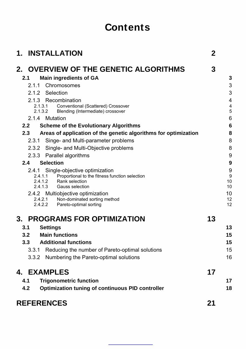
Contents

1. INSTALLATION 2

2. OVERVIEW OF THE GENETIC ALGORITHMS 3 2.1 Main ingredients of GA 3

2.1.1 Chromosomes 3 2.1.2 Selection 3 2.1.3 Recombination 4

2.1.3.1 Conventional (Scattered) Crossover 4 2.1.3.2 Blending (Intermediate) crossover 5

2.1.4 Mutation 6 2.2 Scheme of the Evolutionary Algorithms 6 2.3 Areas of application of the genetic algorithms for optimization 8

2.3.1 Singe- and Multi-parameter problems 8 2.3.2 Single- and Multi-Objective problems 8 2.3.3 Parallel algorithms 9

2.4 Selection 9 2.4.1 Single-objective optimization 9

2.4.1.1 Proportional to the fitness function selection 9 2.4.1.2 Rank selection 10 2.4.1.3 Gauss selection 10

2.4.2 Multiobjective optimization 10 2.4.2.1 Non-dominated sorting method 12 2.4.2.2 Pareto-optimal sorting 12

3. PROGRAMS FOR OPTIMIZATION 13 3.1 Settings 13 3.2 Main functions 15 3.3 Additional functions 15

3.3.1 Reducing the number of Pareto-optimal solutions 15 3.3.2 Numbering the Pareto-optimal solutions 16

4. EXAMPLES 17 4.1 Trigonometric function 17 4.2 Optimization tuning of continuous PID controller 18

REFERENCES 21

2

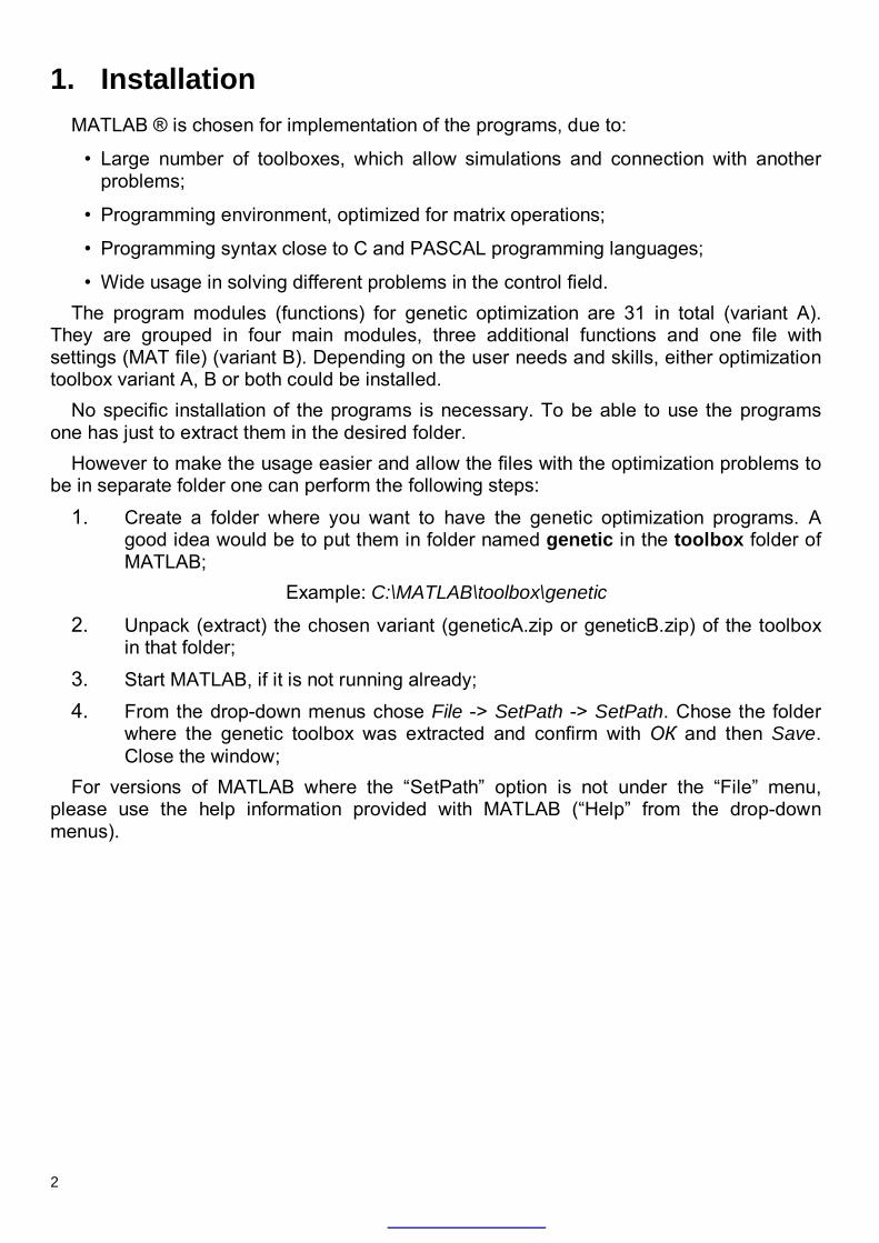
1. Installation MAТLAB ® is chosen for implementation of the programs, due to:

• Large number of toolboxes, which allow simulations and connection with another problems;

• Programming environment, optimized for matrix operations;

• Programming syntax close to C and PASCAL programming languages;

• Wide usage in solving different problems in the control field. The program modules (functions) for genetic optimization are 31 in total (variant A).

They are grouped in four main modules, three additional functions and one file with settings (MAT file) (variant B). Depending on the user needs and skills, either optimization toolbox variant A, В or both could be installed.

No specific installation of the programs is necessary. To be able to use the programs one has just to extract them in the desired folder.

However to make the usage easier and allow the files with the optimization problems to be in separate folder one can perform the following steps:

1. Create a folder where you want to have the genetic optimization programs. A good idea would be to put them in folder named genetic in the toolbox folder of MATLAB;

Example: C:\MATLAB\toolbox\genetic

2. Unpack (extract) the chosen variant (geneticA.zip or geneticB.zip) of the toolbox in that folder;

3. Start MATLAB, if it is not running already;

4. From the drop-down menus chose File -> SetPath -> SetPath. Chose the folder where the genetic toolbox was extracted and confirm with ОК and then Save. Close the window;

For versions of MATLAB where the “SetPath” option is not under the “File” menu, please use the help information provided with MATLAB (“Help” from the drop-down menus).

3

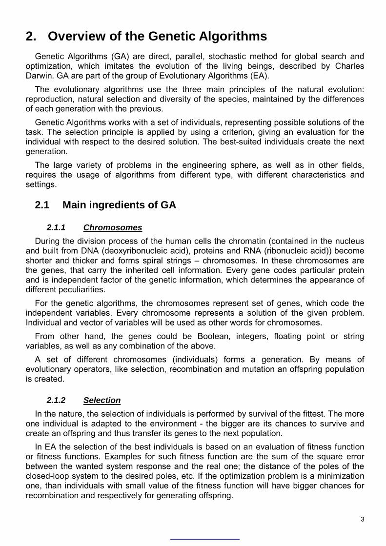
2. Overview of the Genetic Algorithms Genetic Algorithms (GA) are direct, parallel, stochastic method for global search and

optimization, which imitates the evolution of the living beings, described by Charles Darwin. GA are part of the group of Evolutionary Algorithms (EA).

The evolutionary algorithms use the three main principles of the natural evolution: reproduction, natural selection and diversity of the species, maintained by the differences of each generation with the previous.

Genetic Algorithms works with a set of individuals, representing possible solutions of the task. The selection principle is applied by using a criterion, giving an evaluation for the individual with respect to the desired solution. The best-suited individuals create the next generation.

The large variety of problems in the engineering sphere, as well as in other fields, requires the usage of algorithms from different type, with different characteristics and settings.

2.1 Main ingredients of GA

2.1.1 Chromosomes During the division process of the human cells the chromatin (contained in the nucleus

and built from DNA (deoxyribonucleic acid), proteins and RNA (ribonucleic acid)) become shorter and thicker and forms spiral strings – chromosomes. In these chromosomes are the genes, that carry the inherited cell information. Every gene codes particular protein and is independent factor of the genetic information, which determines the appearance of different peculiarities.

For the genetic algorithms, the chromosomes represent set of genes, which code the independent variables. Every chromosome represents a solution of the given problem. Individual and vector of variables will be used as other words for chromosomes.

From other hand, the genes could be Boolean, integers, floating point or string variables, as well as any combination of the above.

A set of different chromosomes (individuals) forms a generation. By means of evolutionary operators, like selection, recombination and mutation an offspring population is created.

2.1.2 Selection In the nature, the selection of individuals is performed by survival of the fittest. The more

one individual is adapted to the environment - the bigger are its chances to survive and create an offspring and thus transfer its genes to the next population.

In EA the selection of the best individuals is based on an evaluation of fitness function or fitness functions. Examples for such fitness function are the sum of the square error between the wanted system response and the real one; the distance of the poles of the closed-loop system to the desired poles, etc. If the optimization problem is a minimization one, than individuals with small value of the fitness function will have bigger chances for recombination and respectively for generating offspring.

4

Methods for single objective and multi-objective optimization are described in sections 2.4.1 and 2.4.2.

2.1.3 Recombination The first step in the reproduction process is the recombination (crossover). In it the

genes of the parents are used to form an entirely new chromosome. The typical recombination for the GA is an operation requiring two parents, but schemes

with more parents area also possible. Two of the most widely used algorithms are Conventional (Scattered) Crossover and Blending (Intermediate) Crossover [ 8 ].

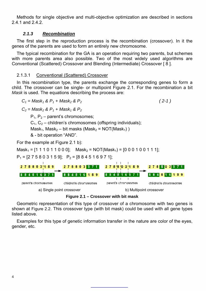
2.1.3.1 Conventional (Scattered) Crossover In this recombination type, the parents exchange the corresponding genes to form a

child. The crossover can be single- or multipoint Figure 2.1. For the recombination a bit Mask is used. The equations describing the process are:

C1 = Mask1 & P1 + Mask2 & P2 ( 2-1 )

C2 = Mask2 & P1 + Mask1 & P2 P1, P2 – parent’s chromosomes; C1, C2 – children’s chromosomes (offspring individuals); Mask1, Mask2 – bit masks (Mask2 = NOT(Mask1) ) & - bit operation “AND”.

For the example at Figure 2.1 b): Mask1 = [1 1 1 0 1 1 0 0 0]; Mask2 = NOT(Mask1) = [0 0 0 1 0 0 1 1 1]; P1 = [2 7 5 8 0 3 1 5 9]; P2 = [8 8 4 5 1 6 9 7 1];

a) Single point crossover b) Multipoint crossover

Figure 2.1 – Crossover with bit mask

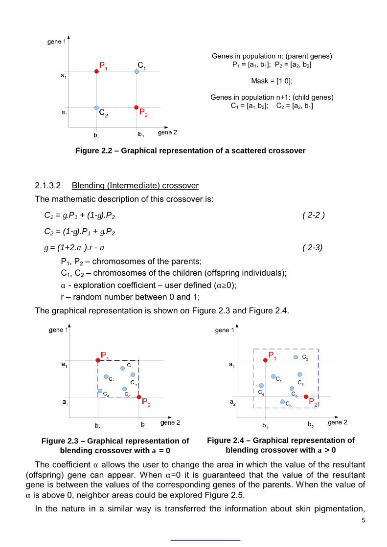
Geometric representation of this type of crossover of a chromosome with two genes is shown at Figure 2.2. This crossover type (with bit mask) could be used with all gene types listed above.

Examples for this type of genetic information transfer in the nature are color of the eyes, gender, etc.

5

2.1.3.2 Blending (Intermediate) crossover The mathematic description of this crossover is:

C1 = γ.P1 + (1-γ).P2 ( 2-2 )

C2 = (1-γ).P1 + γ.P2

γ = (1+2.α ).r - α ( 2-3) P1, P2 – chromosomes of the parents; C1, C2 – chromosomes of the children (offspring individuals); α - exploration coefficient – user defined (α≥0); r – random number between 0 and 1;

The graphical representation is shown on Figure 2.3 and Figure 2.4.

Figure 2.3 – Graphical representation of

blending crossover with α = 0

gene 1

gene 2

P1

P2

a1

a2

b1b2

C1

C2

C3

C5C4

C6

Figure 2.4 – Graphical representation of

blending crossover with α > 0

The coefficient α allows the user to change the area in which the value of the resultant (offspring) gene can appear. When α=0 it is guaranteed that the value of the resultant gene is between the values of the corresponding genes of the parents. When the value of α is above 0, neighbor areas could be explored Figure 2.5.

In the nature in a similar way is transferred the information about skin pigmentation,

Genes in population n: (parent genes) P1 = [a1, b1]; P2 = [a2, b2]

Mask = [1 0];

Genes in population n+1: (child genes)

C1 = [a1, b2]; C2 = [a2, b1]

Figure 2.2 – Graphical representation of a scattered crossover

6

body structure, etc.

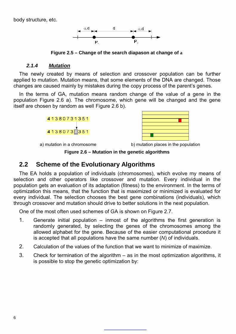
Figure 2.5 – Change of the search diapason at change of α

2.1.4 Mutation The newly created by means of selection and crossover population can be further

applied to mutation. Mutation means, that some elements of the DNA are changed. Those changes are caused mainly by mistakes during the copy process of the parent’s genes.

In the terms of GA, mutation means random change of the value of a gene in the population Figure 2.6 a). The chromosome, which gene will be changed and the gene itself are chosen by random as well Figure 2.6 b).

a) mutation in a chromosome b) mutation places in the population

Figure 2.6 – Mutation in the genetic algorithms

2.2 Scheme of the Evolutionary Algorithms The EA holds a population of individuals (chromosomes), which evolve my means of

selection and other operators like crossover and mutation. Every individual in the population gets an evaluation of its adaptation (fitness) to the environment. In the terms of optimization this means, that the function that is maximized or minimized is evaluated for every individual. The selection chooses the best gene combinations (individuals), which through crossover and mutation should drive to better solutions in the next population.

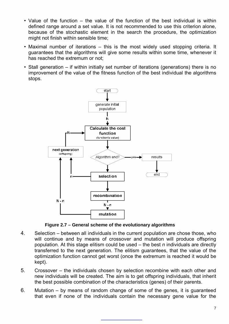
One of the most often used schemes of GA is shown on Figure 2.7.

1. Generate initial population – inmost of the algorithms the first generation is randomly generated, by selecting the genes of the chromosomes among the allowed alphabet for the gene. Because of the easier computational procedure it is accepted that all populations have the same number (N) of individuals.

2. Calculation of the values of the function that we want to minimize of maximize.

3. Check for termination of the algorithm – as in the most optimization algorithms, it is possible to stop the genetic optimization by:

7

• Value of the function – the value of the function of the best individual is within defined range around a set value. It is not recommended to use this criterion alone, because of the stochastic element in the search the procedure, the optimization might not finish within sensible time;

• Maximal number of iterations – this is the most widely used stopping criteria. It guarantees that the algorithms will give some results within some time, whenever it has reached the extremum or not;

• Stall generation – if within initially set number of iterations (generations) there is no improvement of the value of the fitness function of the best individual the algorithms stops.

4. Selection – between all individuals in the current population are chose those, who will continue and by means of crossover and mutation will produce offspring population. At this stage elitism could be used – the best n individuals are directly transferred to the next generation. The elitism guarantees, that the value of the optimization function cannot get worst (once the extremum is reached it would be kept).

5. Crossover – the individuals chosen by selection recombine with each other and new individuals will be created. The aim is to get offspring individuals, that inherit the best possible combination of the characteristics (genes) of their parents.

6. Mutation – by means of random change of some of the genes, it is guaranteed that even if none of the individuals contain the necessary gene value for the

Figure 2.7 – General scheme of the evolutionary algorithms

8

extremum, it is still possible to reach the extremum.

7. New generation – the elite individuals chosen from the selection are combined with those who passed the crossover and mutation, and form the next generation.

2.3 Areas of application of the genetic algorithms for optimization

The Genetic Algorithms are direct, stochastic method for optimization. Since they use populations with allowed solutions (individuals), they count in the group of parallel algorithms. Due to the stochastic was of searching, in most cases, it is necessary to set limits at least for the values of the optimized parameters.

2.3.1 Singe- and Multi-parameter problems Depending on the number of optimized parameters, the problems are divided into:

• Single parameter problem ( )

1minx

f x∈ℜ ( 2-4 )

• Multi-parameter problem ( )min

nxF x

∈ℜ ( 2-5 ) Although that the standard algorithms for genetic optimization are designed for multi-

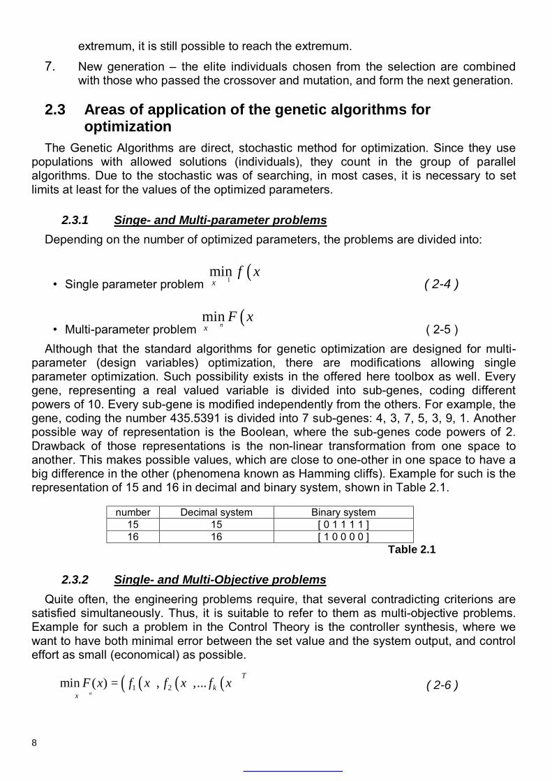
parameter (design variables) optimization, there are modifications allowing single parameter optimization. Such possibility exists in the offered here toolbox as well. Every gene, representing a real valued variable is divided into sub-genes, coding different powers of 10. Every sub-gene is modified independently from the others. For example, the gene, coding the number 435.5391 is divided into 7 sub-genes: 4, 3, 7, 5, 3, 9, 1. Another possible way of representation is the Boolean, where the sub-genes code powers of 2. Drawback of those representations is the non-linear transformation from one space to another. This makes possible values, which are close to one-other in one space to have a big difference in the other (phenomena known as Hamming cliffs). Example for such is the representation of 15 and 16 in decimal and binary system, shown in Table 2.1.

number Decimal system Binary system

15 15 [ 0 1 1 1 1 ] 16 16 [ 1 0 0 0 0 ]

Table 2.1

2.3.2 Single- and Multi-Objective problems Quite often, the engineering problems require, that several contradicting criterions are

satisfied simultaneously. Thus, it is suitable to refer to them as multi-objective problems. Example for such a problem in the Control Theory is the controller synthesis, where we want to have both minimal error between the set value and the system output, and control effort as small (economical) as possible.

( ) ( ) ( )( )1 2min ( ) , ,...н

Tk

xF x f x f x f x

∈ℜ= ( 2-6 )

9

2.3.3 Parallel algorithms Since GA mimic the evolution in the nature, where the search of solution is a parallel

process, GA could by applied, comparatively easy, on parallel computers. There are 3 main ways of doing that:

• Common population, but parallel evaluation of the fitness function – the fitness function of each individual is evaluated on separate (in the best case) processor (slave), where as the genetic operators are applied on another processor (master);

• Division to subpopulations – the whole population is divided into sub-populations, which are assigned to separate processors;

• Spreading of the genetic operations (modification of “division to subpopulations”) – the genetic operators are applied between “neighbor” populations. This allows keeping the diversity of the species.

2.4 Selection As it was explained above, the selection is a process, in which the individuals which will

be applied to the genetic operations and which will create the offspring population are chosen. The selection has two main purposes:

1. To chose the most perspective individuals, which will take part in the generation of next population or will be directly copied (elitism);

2. To give an opportunity to an individuals with comparatively bad value of the fitness function/functions to take part in the creation process of the next generation. This allows us to preserve the global character of the search process and not allow a single individual to dominate the population and thus bring it to local extremum.

2.4.1 Single-objective optimization In this case, we have only one function, which we want to optimize. For each individual

in the generation the fitness value is evaluated and later used to choose those individuals, which will create the next generation.

In the offered toolbox, there are three methods of selection:

2.4.1.1 Proportional to the fitness function selection The probability (P) of each individual to be selected is calculated as the proportion of its

fitness function to the sum of the fitness functions of all individuals in the current generation. It should be noted, that this type of selection is for maximization problems, whereas the toolbox searches always for the minimum. This is done by recalculating the fitness values in such a way, that the best individuals (minimal function value) receive the maximal fitness and vice versa.

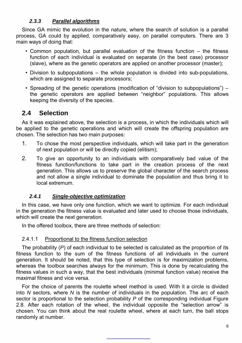
For the choice of parents the roulette wheel method is used. With it a circle is divided into N sectors, where N is the number of individuals in the population. The arc of each sector is proportional to the selection probability P of the corresponding individual Figure 2.8. After each rotation of the wheel, the individual opposite the “selection arrow” is chosen. You can think about the real roulette wheel, where at each turn, the ball stops randomly at number.

10

In the programs, a linear representation of the roulette wheel Figure 2.9 and a random number generator within [0,1) are used. This random number is multiplied by the sum of the fitness functions for the generation and bottom-up addition is started (I-1, I-2, I-3, …), until the sum of the numbers exceed the random number. The index of the last added fitness function is taken and added to the parents set for the next gene.

This selection method however has a disadvantage in case that one of several individuals has fitness function, which is in magnitudes better than the others. In that case, those individual/individuals will dominate the generation and will cause convergence to a point, which could be far from the optimum. The next two methods try to solve this problem.

2.4.1.2 Rank selection The individuals are sorted according to the value of their fitness function and than they

are assigned a rank. The rank of the best individual is 1, of the second best 2 and so on. The selection probability for each individual is calculated according the following non-linear function:

P = β.(1– β)(rank – 1) ( 2-7 )

Where β is a user defined coefficient. For the selection is used the method of the roulette wheel.

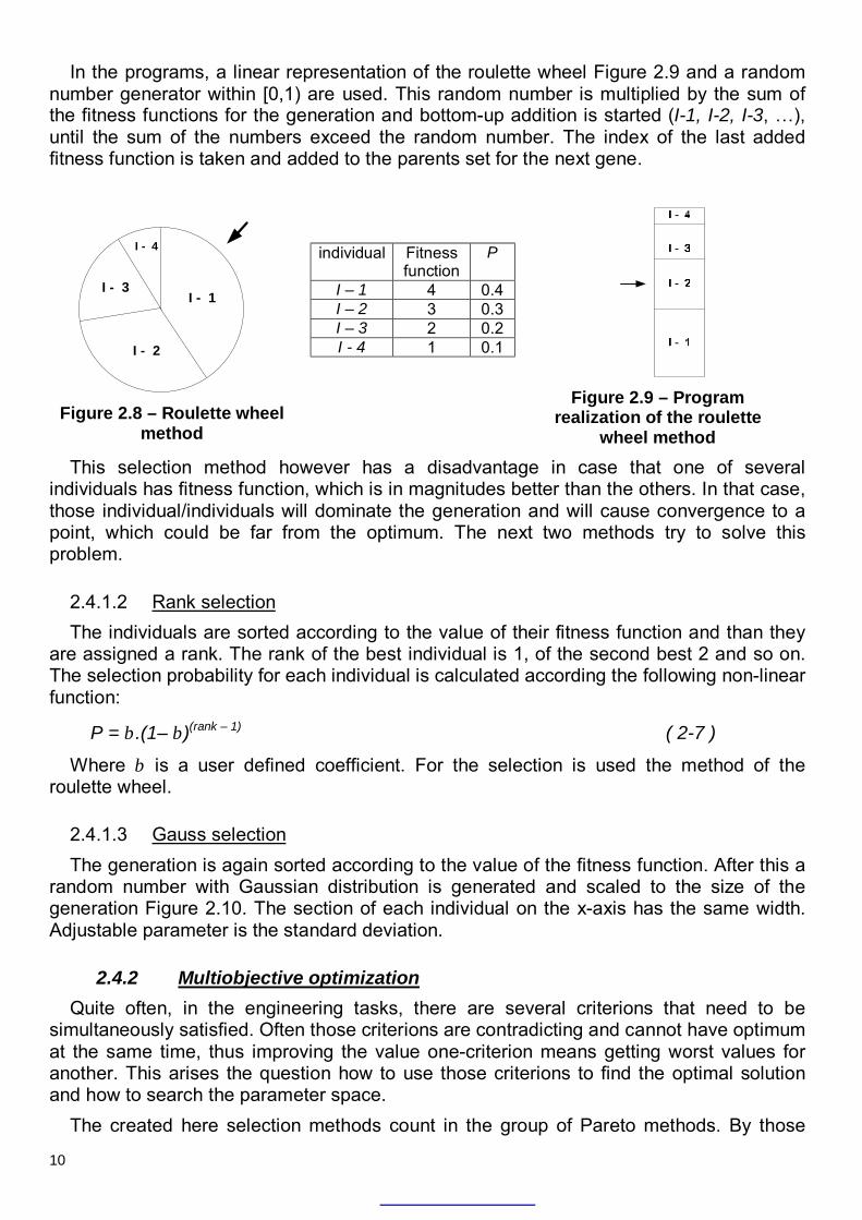
2.4.1.3 Gauss selection The generation is again sorted according to the value of the fitness function. After this a

random number with Gaussian distribution is generated and scaled to the size of the generation Figure 2.10. The section of each individual on the x-axis has the same width. Adjustable parameter is the standard deviation.

2.4.2 Multiobjective optimization Quite often, in the engineering tasks, there are several criterions that need to be

simultaneously satisfied. Often those criterions are contradicting and cannot have optimum at the same time, thus improving the value one-criterion means getting worst values for another. This arises the question how to use those criterions to find the optimal solution and how to search the parameter space.

The created here selection methods count in the group of Pareto methods. By those

I - 1

I - 2

I - 3

I - 4

Figure 2.8 – Roulette wheel

method

individual Fitness function

P

I – 1 4 0.4 I – 2 3 0.3 I – 3 2 0.2 I - 4 1 0.1

Figure 2.9 – Program

realization of the roulette wheel method

11

types of methods a set of non-dominated solutions is obtained, from which the user could chose the one that best suits the requirements and needs.

Let is assume we have k objective functions we want to minimize:

( ) ( ) ( )( )1 2min ( ) , ,...н

Tk

xF x f x f x f x

∈ℜ=

( 2-8 )

Definition 1: Dominating: Vector v is said to dominate vector u, if:

{ } ( ) ( )1, 2... : i ii k f v f u∀ ∈ ≤ and { } ( ) ( )1, 2... : j jj k f v f u∃ ∈ < ( 2-9 ),

thus for at least one fitness function v is giving smaller value than u.

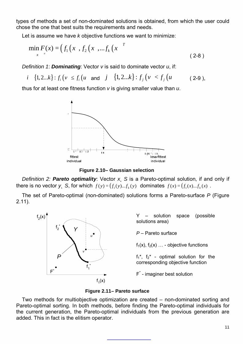
Definition 2: Pareto optimality: Vector x∈S is a Pareto-optimal solution, if and only if there is no vector y∈S, for which ( ))()...()( 1 yfyfyf k= dominates ( ))()...()( 1 xfxfxf k= .

The set of Pareto-optimal (non-dominated) solutions forms a Pareto-surface P (Figure 2.11).

Two methods for multiobjective optimization are created – non-dominated sorting and Pareto-optimal sorting. In both methods, before finding the Pareto-optimal individuals for the current generation, the Pareto-optimal individuals from the previous generation are added. This in fact is the elitism operator.

Figure 2.10– Gaussian selection

f2(x)

f1(x)

P

Yf2*

f1*

F*

v

u

Y – solution space (possible solutions area)

P – Pareto surface

f1(x), f2(x) … - objective functions

f1*, f2* - optimal solution for the corresponding objective function

F* - imaginer best solution

Figure 2.11– Pareto surface

12

2.4.2.1 Non-dominated sorting method The individuals in the population are sorted and the Pareto-surface is found. All non-

dominated individuals in the population receive the same rank (1). Then they are taken out and the rest of the population is sorted again. Again, a Pareto-surface is found and the individuals forming it receive rank 2. The process is repeated until all individuals receive rank - Figure 2.12. Than the ranks are recalculated, so the rank of the individuals on the first Pareto-surface gets maximal. The roulette wheel method is used.

2.4.2.2 Pareto-optimal sorting From all individuals in the current generation only the Pareto-optimal are taken. At

Figure 2.13 those are A, B and C. The recombine with each other and generate the next generation. When there is only one individual that dominates the whole generation, than also the second Pareto-surface is found and used for the recombination. Drawback of this method is that several individuals “steer” the search and the algorithm can stuck in local minima. Advantages toward the non-dominated sorting are the fastest selection and convergence.

In both methods the number of Pareto-optimal (for the generation) individuals is limited, when it exceeds the defined number. This is done by calculating a function of closeness between the individuals:

min min( )

2i kx x x x

D x− + −

= ( 2-10 )

where x≠xi≠xk≠x are individuals on the Pareto-surface. The individual with smaller value of D (distance to the other points) is removed. This

process continues until the desired number of points is achieved. Beside limiting the number of points this helps to keep the diversity of the Pareto-set and obtain better spread surface.

Figure 2.12 – Non-dominated sorting

method

Figure 2.13 – Pareto-optimal sorting

method

13

3. Programs for optimization Totally four optimization algorithms are developed (Table 3.1). The algorithms are

modules based, which eases adding and exchanging genetic operators, visualization modules, etc. The Blend Crossover (BC) have the possibility for extended representation of the genes.

Single objective Multiobjective

Standard (scattered) crossover

GAminSC GAМОminSC

Blending (intermediate)

crossover GAminBC GAМОminBC

Table 3.1

3.1 Settings All algorithms use the same structure of definition of the parameters. This is realized by

GAopt program, which allows loading, changing and saving of the user settings. The possible settings are:

name type description

MaxIter integer Number of generations (iterations) of the optimization. This is

the only stopping criterion.

PopulSize integer Population size – number of individuals (chromosomes) in the

population.

MutatRate

real ≥ 0 Percentage of the individuals, which will mutate (rounded to an integer number). When extended gene representation (see Section ???) is used, the coefficientк is scaled by the percentage of gene enlargement.

BestRate

real ∈[0,1] For single-objective optimization this is percentage from the population, which is copied to the next generation without changes (elite coefficient). For multiobjective optimization this defines the maximal number of Pareto-surface individuals as: Pareto_individuals = max(3, round(PopulSize.BestRate)) Thus the minimal number of individuals is 3.

NewRate Real ∈(0,1) Percentage from the generation, which is filled with newly created individuals.

TolX

real > 0;

0

-1

When TolX > 0, it defines the precision for the variables (Example: TolX = 1e-4 means that the variables are evaluated with precision up to 0,0001). When TolX = 0, floating point variable representation is used. Tox = -1 mean that the variables can take only integer values.

pSelect real Selection parameter – depends on the used selection type.

14

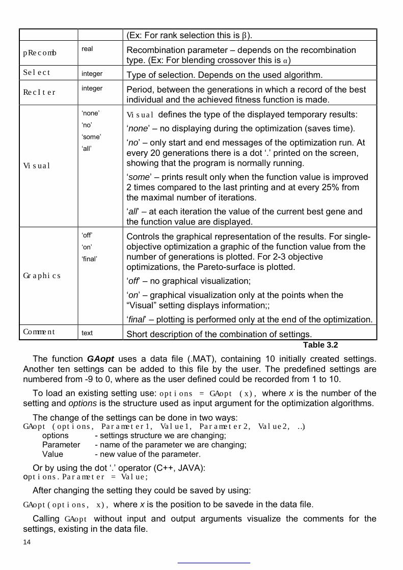
(Ex: For rank selection this is β).

pRecomb real Recombination parameter – depends on the recombination

type. (Ex: For blending crossover this is α) Select integer Type of selection. Depends on the used algorithm.

RecIter integer Period, between the generations in which a record of the best

individual and the achieved fitness function is made.

Visual

‘none’

‘no’

‘some’

‘all’

Visual defines the type of the displayed temporary results: ‘none’ – no displaying during the optimization (saves time). ‘no’ – only start and end messages of the optimization run. At every 20 generations there is a dot ‘.’ printed on the screen, showing that the program is normally running. ‘some’ – prints result only when the function value is improved 2 times compared to the last printing and at every 25% from the maximal number of iterations. ‘all’ – at each iteration the value of the current best gene and the function value are displayed.

Graphics

‘off’

‘on’

‘final’

Controls the graphical representation of the results. For single-objective optimization a graphic of the function value from the number of generations is plotted. For 2-3 objective optimizations, the Pareto-surface is plotted. ‘off’ – no graphical visualization; ‘on’ – graphical visualization only at the points when the “Visual” setting displays information;; ‘final’ – plotting is performed only at the end of the optimization.

Comment text Short description of the combination of settings. Table 3.2

The function GAopt uses a data file (.MAT), containing 10 initially created settings. Another ten settings can be added to this file by the user. The predefined settings are numbered from -9 to 0, where as the user defined could be recorded from 1 to 10.

To load an existing setting use: options = GAopt (x), where x is the number of the setting and options is the structure used as input argument for the optimization algorithms.

The change of the settings can be done in two ways: GAopt (options, Parameter1, Value1, Parameter2, Value2, …)

options - settings structure we are changing; Parameter - name of the parameter we are changing; Value - new value of the parameter.

Or by using the dot ‘.’ operator (C++, JAVA): оptions.Parameter = Value;

After changing the setting they could be saved by using: GAopt(options, x), where x is the position to be savedе in the data file.

Calling GAopt without input and output arguments visualize the comments for the settings, existing in the data file.

15

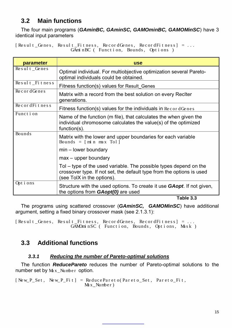
3.2 Main functions The four main programs (GAminBC, GAminSC, GAMOminBC, GAMOMinSC) have 3

identical input parameters [Result_Genes, Result_Fitness, RecordGenes, RecordFitness] = ...

GAminBC ( Function, Bounds, Options )

parameter use Result_Genes

Optimal individual. For multiobjective optimization several Pareto-optimal individuals could be obtained.

Result_Fitness Fitness function(s) values for Result_Genes

RecordGenes Matrix with a record from the best solution on every RecIter generations.

RecordFitness Fitness function(s) values for the individuals in RecordGenes

Function Name of the function (m file), that calculates the when given the individual chromosome calculates the value(s) of the optimized function(s).

Bounds Matrix with the lower and upper boundaries for each variable Bounds = [min max Tol]

min – lower boundary max – upper boundary Tol – type of the used variable. The possible types depend on the crossover type. If not set, the default type from the options is used (see TolX in the options).

Options Structure with the used options. To create it use GAopt. If not given, the options from GAopt(0) are used

Table 3.3

The programs using scattered crossover (GAminSC, GAMOMinSC) have additional argument, setting a fixed binary crossover mask (see 2.1.3.1): [Result_Genes, Result_Fitness, RecordGenes, RecordFitness] = ...

GAMOminSC ( Function, Bounds, Options, Mask )

3.3 Additional functions

3.3.1 Reducing the number of Pareto-optimal solutions The function ReducePareto reduces the number of Pareto-optimal solutions to the

number set by Max_Number option. [New_P_Set, New_P_Fit] = ReducePareto(Pareto_Set, Pareto_Fit,

Max_Number)

16

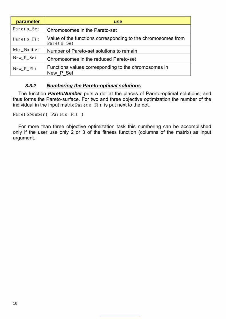
parameter use Pareto_Set Chromosomes in the Pareto-set

Pareto_Fit Value of the functions corresponding to the chromosomes from Pareto_Set

Max_Number Number of Pareto-set solutions to remain New_P_Set Chromosomes in the reduced Pareto-set

New_P_Fit Functions values corresponding to the chromosomes in New_P_Set

3.3.2 Numbering the Pareto-optimal solutions The function ParetoNumber puts a dot at the places of Pareto-optimal solutions, and

thus forms the Pareto-surface. For two and three objective optimization the number of the individual in the input matrix Pareto_Fit is put next to the dot. ParetoNumber( Pareto_Fit )

For more than three objective optimization task this numbering can be accomplished only if the user use only 2 or 3 of the fitness function (columns of the matrix) as input argument.

17

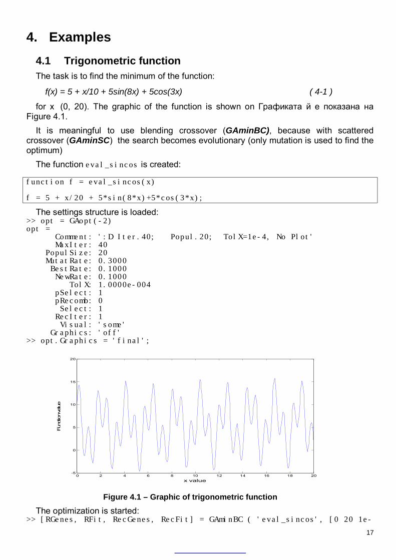
4. Examples 4.1 Trigonometric function The task is to find the minimum of the function:

f(x) = 5 + x/10 + 5sin(8x) + 5cos(3x) ( 4-1 )

for x∈(0, 20). The graphic of the function is shown on Графиката й е показана на Figure 4.1.

It is meaningful to use blending crossover (GAminBC), because with scattered crossover (GAminSC) the search becomes evolutionary (only mutation is used to find the optimum)

The function eval_sincos is created: function f = eval_sincos(x) f = 5 + x/20 + 5*sin(8*x)+5*cos(3*x);

The settings structure is loaded: >> opt = GAopt(-2) opt = Comment: ':D Iter.40; Popul.20; TolX=1e-4, No Plot' MaxIter: 40 PopulSize: 20 MutatRate: 0.3000 BestRate: 0.1000 NewRate: 0.1000 TolX: 1.0000e-004 pSelect: 1 pRecomb: 0 Select: 1 RecIter: 1 Visual: 'some' Graphics: 'off' >> opt.Graphics = 'final';

0 2 4 6 8 10 12 14 16 18 20-5

0

5

10

15

20

x value

Func

tion va

lue

Figure 4.1 – Graphic of trigonometric function

The optimization is started: >> [RGenes, RFit, RecGenes, RecFit] = GAminBC ( 'eval_sincos', [0 20 1e-

18

4], opt); GENETIC ALGORITHM for MATLAB, ver 1.0 Minimization of function "eval_sincos" ->Iter:40 Popul:20<- Started at 14:42:32 29.6.2003 Iter: Fit: Gen: 1 -4.33242 11.5715 10 -4.33964 5.3347 20 -4.56185 5.3154 30 -4.56185 5.3154 40 -4.65082 5.2943 Fitness Value: -4.650824 Result Genes: 5.2943

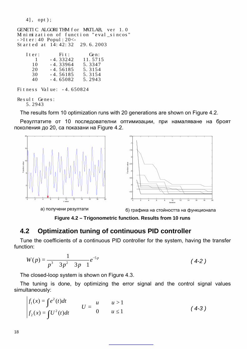
The results form 10 optimization runs with 20 generations are shown on Figure 4.2. Резултатите от 10 последователни оптимизации, при намаляване на броят

поколения до 20, са показани на Figure 4.2.

0 2 4 6 8 10 12 14 16 18 20-5

0

5

10

15

20

x value

Func

tion

valu

e

а) получени резултати

0 2 4 6 8 10 12 14 16 18 20-5

-4.5

-4

-3.5

-3

-2.5

-2

-1.5

-1

-0.5

iteration

Func

tion

valu

e

б) графика на стойността на функционала

Figure 4.2 – Trigonometric function. Results from 10 runs

4.2 Optimization tuning of continuous PID controller Tune the coefficients of a continuous PID controller for the system, having the transfer

function:

53 2

1( )3 3 1

pW p ep p p

−=+ + + ( 4-2 )

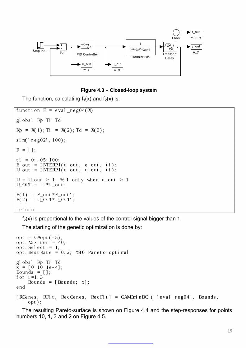
The closed-loop system is shown on Figure 4.3. The tuning is done, by optimizing the error signal and the control signal values

simultaneously: 2

1

22

( ) ( ) 10 1( ) ( )

f x e t dt u uU

uf x U t dt

= >= ≤=

∫∫

( 4-3 )

19

The function, calculating f1(x) and f2(x) is:

function F = eval_reg04(X) global Kp Ti Td Kp = X(1);Ti = X(2);Td = X(3); sim('reg02',100); F = []; ti = 0:.05:100; E_out = INTERP1(t_out, e_out, ti); U_out = INTERP1(t_out, u_out, ti); U = U_out > 1; % 1 only when u_out > 1 U_OUT = U.*U_out; F(1) = E_out*E_out'; F(2) = U_OUT*U_OUT'; return

f2(x) is proportional to the values of the control signal bigger than 1. The starting of the genetic optimization is done by:

opt = GAopt(-5); opt.MaxIter = 40; opt.Select = 1; opt.BestRate = 0.2; %10 Pareto optimal global Kp Ti Td x = [0 10 1e-4]; Bounds = []; for i=1:3 Bounds = [Bounds; x]; end [RGenes, RFit, RecGenes, RecFit] = GAMOminBC ( 'eval_reg04', Bounds,

opt);

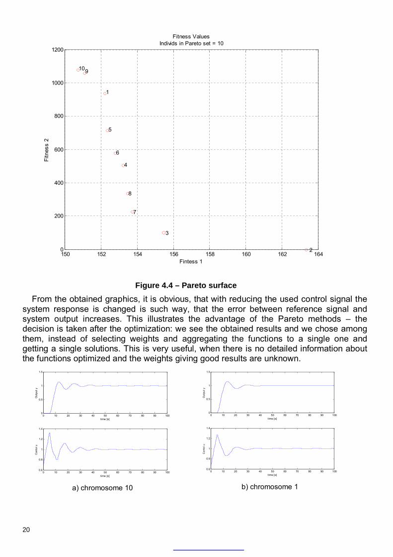
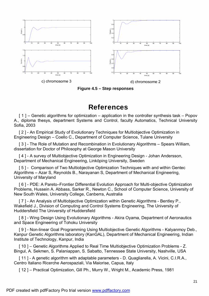
The resulting Pareto-surface is shown on Figure 4.4 and the step-responses for points numbers 10, 1, 3 and 2 on Figure 4.5.

y_out

w_y

u_out

w_u

t_out

w_time

e_out

w_e

TransportDelay

1

s +3s +3s+13 2

Transfer FcnSumStep Input

PID Control ler

Clock

Figure 4.3 – Closed-loop system

20

150 152 154 156 158 160 162 1640

200

400

600

800

1000

1200

Fitness ValuesIndivids in Pareto set = 10

Fintess 1

Fitn

ess

2

1

2

3

4

5

6

7

8

910

Figure 4.4 – Pareto surface

From the obtained graphics, it is obvious, that with reducing the used control signal the system response is changed is such way, that the error between reference signal and system output increases. This illustrates the advantage of the Pareto methods – the decision is taken after the optimization: we see the obtained results and we chose among them, instead of selecting weights and aggregating the functions to a single one and getting a single solutions. This is very useful, when there is no detailed information about the functions optimized and the weights giving good results are unknown.

0 10 20 30 40 50 60 70 80 90 1000

0.5

1

1.5

time [s]

Out

put y

0 10 20 30 40 50 60 70 80 90 1000.6

0.8

1

1.2

1.4

time [s]

Con

tol u

a) chromosome 10

0 10 20 30 40 50 60 70 80 90 1000

0.5

1

1.5

time [s]

Out

put y

0 10 20 30 40 50 60 70 80 90 1000.6

0.8

1

1.2

1.4

time [s]

Con

tol u

b) chromosome 1

21

0 10 20 30 40 50 60 70 80 90 1000

0.5

1

1.5

time [s]

Out

put y

0 10 20 30 40 50 60 70 80 90 1000.6

0.8

1

1.2

1.4

time [s]

Cont

ol u

c) chromosome 3

0 10 20 30 40 50 60 70 80 90 1000

0.2

0.4

0.6

0.8

1

time [s]

Out

put y

0 10 20 30 40 50 60 70 80 90 1000.5

0.6

0.7

0.8

0.9

1

time [s]

Con

tol u

d) chromosome 2

Figure 4.5 – Step responses

References [ 1 ] – Genetic algorithms for optimization – application in the controller synthesis task – Popov

A., diploma thesys, department Systems and Control, faculty Automatics, Technical University Sofia, 2003

[ 2 ] - An Empirical Study of Evolutionary Techniques for Multiobjective Optimization in Engineering Design – Coello C., Department of Computer Science, Tulane University

[ 3 ] - The Role of Mutation and Recombination in Evolutionary Algorithms – Spears William, dissertation for Doctor of Philosophy at George Mason University

[ 4 ] - A survey of Multiobjective Optimization in Engineering Design - Johan Andersson, Department of Mechanical Engineering, Linköping University, Sweden

[ 5 ] - Comparison of Two Multiobjective Optimization Techniques with and within Gentec Algorithms – Azar S, Reynolds B., Narayanan S, Department of Mechanical Engineering, University of Maryland

[ 6 ] - PDE: A Pareto–Frontier Differential Evolution Approach for Multi-objective Optimization Problems, Hussein A. Abbass, Sarker R., Newton C., School of Computer Science, University of New South Wales, University College, Canberra, Australia

[ 7 ] - An Analysis of Multiobjective Optimization within Genetic Algorithms - Bentley P., Wakefield J., Division of Computing and Control Systems Engineering, The University of Huddersfield The University of Huddersfield

[ 8 ] - Wing Design Using Evolutionary Algorithms - Akira Oyama, Department of Aeronautics and Space Engineering of Tohoku University

[ 9 ] - Non-linear Goal Programming Using Multiobjective Genetic Algorithms - Kalyanmoy Deb., Kanpur Genetic Algorithms laboratory (KanGAL), Department of Mechanical Engineering, Indian Institute of Technology, Kanpur, India

[ 10 ] – Genetic Algorithms Applied to Real Time Multiobjective Optimization Problems - Z. Bingul, A. Sekmen, S. Palaniappan, S. Sabatto, Tennessee State University, Nashville, USA

[ 11 ] - A genetic algorithm with adaptable parameters - D. Quagliarella, A. Vicini, C.I.R.A., Centro Italiano Ricerche Aerospaziali, Via Maiorise, Capua, Italy

[ 12 ] – Practical Optimization, Gill Ph., Murry W., Wright M., Academic Press, 1981

PDF created with pdfFactory Pro trial version www.pdffactory.com

Genetic Algorithms for Optimization Programs for MATLAB

Andrey Popov andrey.popov@gmx.net www.automatics.hit.bg

TU – Sofia

2003