genetic algorithms -...
TRANSCRIPT
Genetic Algorithms
John BurkardtDepartment of Scientific Computing
Florida State University..........
Mathematics Department Undergraduate SeminarTrinity University
http://people.sc.fsu.edu/∼jburkardt/presentations/...genetic 2013 trinity.pdf
21 February 2013
1 / 50
Reference
Zbigniew Michalewicz,Genetic Algorithms + Data Structures = Evolution Programs,Third Edition,Springer, 1996,ISBN: 3-540-60676-9,LC: QA76.618.M53.
Nick Berry,A “Practical” Use for Genetic Programming,http://www.datagenetics.com/blog.html
John Burkardt,Approximate an Image Using a Genetic Algorithm,http://people.sc.fsu.edu/∼/jburkardt/m src/image match genetic/image match genetic.html
John Burkardt,A Simple Genetic Algorithm,http://people.sc.fsu.edu/∼/jburkardt/cpp src/simple ga/simple ga.html
Christopher Houck, Jeffery Joines, Michael Kay,A Genetic Algorithm for Function Optimization: A Matlab Implementation,NCSU-IE Technical Report 95-09, 1996.
The Mathworks,Global Optimization Toolbox,http://www.mathworks.com/products/global-optimization/index.html
2 / 50
Genetic Algorithms
Introduction
Genetic Algorithms
A Simple Optimization
The Patchwork Picture
Conclusion
3 / 50
Introduction - Computers Implement “Recipes”
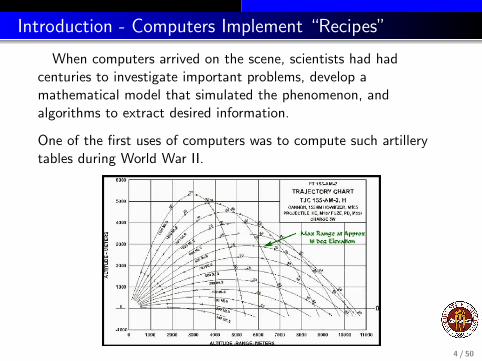
When computers arrived on the scene, scientists had hadcenturies to investigate important problems, develop amathematical model that simulated the phenomenon, andalgorithms to extract desired information.
One of the first uses of computers was to compute such artillerytables during World War II.
4 / 50

Introduction - Knock Down the Steeple
The flight of a cannon ball can be modeled as a mathematicalparabola, with three degrees of freedom. The location and angle ofthe cannon determine two degrees and the amount of gun powderthe third. By experiment, we can create tables that tell us whetherwe can hit the steeple, and if so, the minimum amount ofgunpowder to use, and how to aim the cannon.
5 / 50
Introduction - Harder Problems
Thus, people tried to solve problems by understanding the modelwell enough to be able to see how a solution could be produced,and then implementing that procedure as an algorithm.
* Fourier developed a model of signals as sums of sines and cosines,and now we can solve heat conduction problems, and electricalengineers create electronic circuits with any desired property.
* Linear programming was able to solve many scheduling problemsfor airlines and allocation problems for factories.
But what happens when we find a problem that needs to besolved, but for which we simply cannot see an efficient way todetermine a solution?
There are lots of problems like that!
6 / 50
Introduction - The Traveler
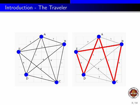
One simple problem involves a traveler who must visit plan around trip that visits each city on a list once. The traveler is freeto choose the order in which the cities are visited and wishes tofind the route that minimizes the total mileage.
This problem is easy to state and understand, versions of it comeup all the time in many situations, and yet there isno efficient algorithm for solving it!
The only sure way to find the best route is to check every possiblelist. For n cities, that means n! possible itineraries.
On the other hand, given two itineraries, it is certainly easy tocheck which one is better - just compare the mileages.
7 / 50
Introduction - The Traveler
8 / 50
Introduction - The Patchwork Picture
Here’s another simple problem: suppose you want to make acopy of a famous photograph or painting, but you are only able touse colored rectangles. You have rectangles in every size and color.The rectangles are transparent, and if two overlap, the overlappingregion will have the average of the two colors.
If that was the whole problem, we’d be done, because we makepixellated versions of images all the time.
But for this problem, we are only allowed to use 32 rectangles!
Suddenly, your mind goes blank. There’s no obvious solution.
But given any two attempts to copy the picture, we can alwaysdetermine which one is better, essentially by measuring thedifference between the original and the copies.
9 / 50
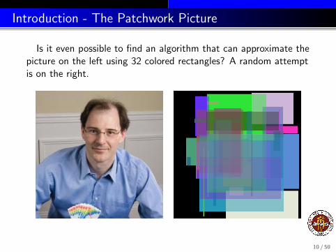
Introduction - The Patchwork Picture
Is it even possible to find an algorithm that can approximate thepicture on the left using 32 colored rectangles? A random attemptis on the right.
10 / 50
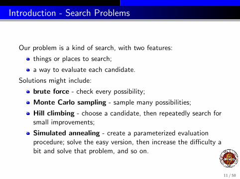
Introduction - Search Problems
Our problem is a kind of search, with two features:
things or places to search;
a way to evaluate each candidate.
Solutions might include:
brute force - check every possibility;
Monte Carlo sampling - sample many possibilities;
Hill climbing - choose a candidate, then repeatedly search forsmall improvements;
Simulated annealing - create a parameterized evaluationprocedure; solve the easy version, then increase the difficulty abit and solve that problem, and so on.
11 / 50
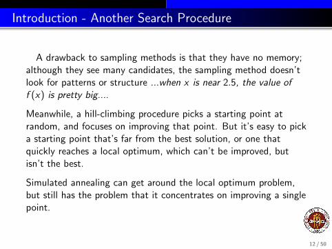
Introduction - Another Search Procedure
A drawback to sampling methods is that they have no memory;although they see many candidates, the sampling method doesn’tlook for patterns or structure ...when x is near 2.5, the value off (x) is pretty big....
Meanwhile, a hill-climbing procedure picks a starting point atrandom, and focuses on improving that point. But it’s easy to picka starting point that’s far from the best solution, or one thatquickly reaches a local optimum, which can’t be improved, butisn’t the best.
Simulated annealing can get around the local optimum problem,but still has the problem that it concentrates on improving a singlepoint.
12 / 50

Genetic Algorithms
Introduction
Genetic Algorithms
A Simple Optimization
The Patchwork Picture
Conclusion
13 / 50
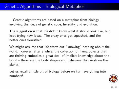
Genetic Algorithms - Biological Metaphor
Genetic algorithms are based on a metaphor from biology,involving the ideas of genetic code, heredity, and evolution.
The suggestion is that life didn’t know what it should look like, butkept trying new ideas. The crazy ones got squashed, and thebetter ones flourished.
We might assume that life starts out “knowing” nothing about theworld; however, after a while, the collection of living objects thatare thriving embodies a great deal of implicit knowledge about theworld - these are the body shapes and behaviors that work on thisplanet.
Let us recall a little bit of biology before we turn everything intonumbers!
14 / 50
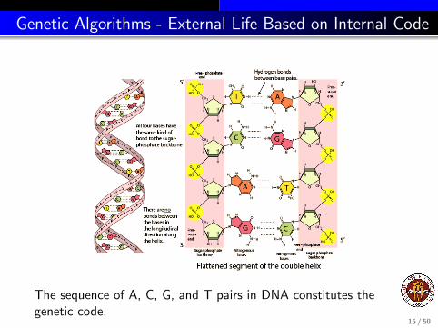
Genetic Algorithms - External Life Based on Internal Code
The sequence of A, C, G, and T pairs in DNA constitutes thegenetic code.
15 / 50
Genetic Algorithms: Fitness, Survival, Modification
In our idealized model of biology, we notice that within aspecies, individuals exhibit a variety of traits.
We can explain these differences by looking at the geneticinformation carried by each individual. For a given species, we canthink of the genetic information as being a list, of a fixed length,containing certain allowed “digits”, perhaps A, C, G, T.
Two individuals of the same species, with different geneticinformation, will have different properties and abilities, and thesedifferences will influence their relative fitness to survive.
Individuals that are more fit are more likely to survive and to breed.
Breeding requires two individuals, and involves the somewhatrandom selection of genetic information from each.
Changes in genetic information can also occur because ofspontaneous mutation.
16 / 50
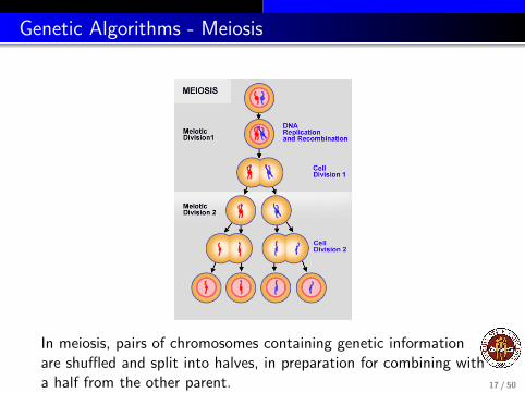
Genetic Algorithms - Meiosis
In meiosis, pairs of chromosomes containing genetic informationare shuffled and split into halves, in preparation for combining witha half from the other parent. 17 / 50
Genetic Algorithms - Meiosis
Suppose we could measure the fitness of an individual named xfor the given environment, producing a rating f (x) which is higherfor fitter individuals.
Then we could regard a population of individuals as an initiallyrandom sample of x values. In a “struggle” to eat, hold territory,and mate, the weaker individuals would be likely to die, theirgenetic information discarded.
Those individuals with the highest f (x) values are preferentiallyallowed to reproduce - but reproduction involves shuffling thegenetic information of two fit individuals to produce a new anddifferent individual.
Over time, one might hope that the population of x values wouldevolve so that the values of f (x) would increase, perhaps up tosome limiting value.
18 / 50
Genetic Algorithms: The Genetic Algorithm Idea
A genetic algorithm is a kind of optimization procedure. From agiven population X , it seeks the item x ∈ X which has the greatest“fitness”, that is, the maximum value of f (x).
A genetic algorithm searches for the best value by creating a smallpool of random candidates, selecting the best candidates, andallowing them to “breed”, with minor variations, repeating thisprocess over many generations.
These ideas are all inspired by the analogy with the evolution ofliving organisms.
19 / 50
Genetic Algorithms: Algorithmic Structure
A genetic algorithm typically includes:
1 a genetic representation of candidates;
2 a way to create an initial population of candidates;
3 a function measuring the “fitness” of each candidate;
4 a generation step, in which some candidates “die”, somesurvive, others reproduce by breeding;
5 a mechanism that recombines genes from breeding pairs, andmutates others.
20 / 50
Genetic Algorithms: Choosing a Representation
The part of the genetic algorithm that varies the most fromproblem to problem will be the representation of the candidates.
Even for the traveling salesman problem, it’s not too hard to seehow to make this representation numeric - we can number thecities and then an itinerary simply lists those numbers in aparticular order.
However, in order to make the breeding and mutation work, we willneed to be able to convert the representation, whatever it is, backand forth to a binary representation, that is, a sequence of 0’s and1’s.
This has to be done in such a way that if we change one bit of thebinary information, we are still describing a candidate.
21 / 50
Genetic Algorithms
Introduction
Genetic Algorithms
A Simple Optimization
The Patchwork Picture
Conclusion
22 / 50
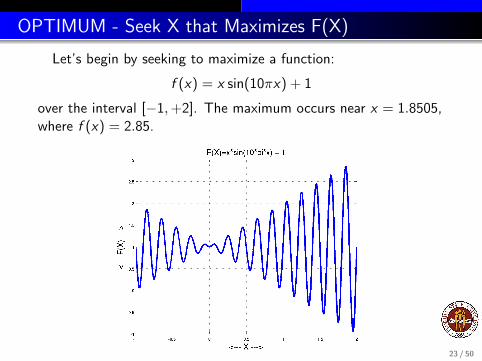
OPTIMUM - Seek X that Maximizes F(X)
Let’s begin by seeking to maximize a function:
f (x) = x sin(10πx) + 1
over the interval [−1,+2]. The maximum occurs near x = 1.8505,where f (x) = 2.85.
23 / 50
OPTIMUM - Using Other Algorithms
To get six decimal places of accuracy, there are 3, 000, 000distinct values in [−1,+2] we must consider.
A Monte Carlo scheme would have to sample perhaps 100,000values before having a chance to find the right value.
A hill climbing scheme would have to start near the solution, or itwill climb up one of the lesser mountains.
Our genetic algorithm will assume the solution can be coded usingbinary data, and will try to find that code using “evolution”.
24 / 50
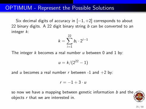
OPTIMUM - Represent the Possible Solutions
Six decimal digits of accuracy in [−1,+2] corresponds to about22 binary digits. A 22 digit binary string b can be converted to aninteger k :
k =22∑i=1
bi · 2i−1
The integer k becomes a real number u between 0 and 1 by:
u = k/(222 − 1)
and u becomes a real number r between -1 and +2 by:
r = −1 + 3 · u
so now we have a mapping between genetic information b and theobjects r that we are interested in.
25 / 50
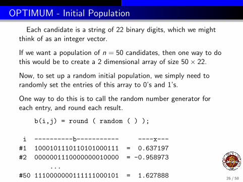
OPTIMUM - Initial Population
Each candidate is a string of 22 binary digits, which we mightthink of as an integer vector.
If we want a population of n = 50 candidates, then one way to dothis would be to create a 2 dimensional array of size 50× 22.
Now, to set up a random initial population, we simply need torandomly set the entries of this array to 0’s and 1’s.
One way to do this is to call the random number generator foreach entry, and round each result.
b(i,j) = round ( random ( ) );
i ----------b----------- ----x---#1 1000101110110101000111 = 0.637197#2 0000001110000000010000 = -0.958973
...#50 1110000000111111000101 = 1.627888 26 / 50
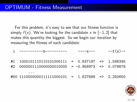
OPTIMUM - Fitness Measurement
For this problem, it’s easy to see that our fitness function issimply f (x). We’re looking for the candidate x in [−1, 2] thatmakes this quantity the biggest. So we begin our iteration bymeasuring the fitness of each candidate:
i -----------b---------- ----x--- --f(x)--
#1 1000101110110101000111 = 0.637197 => 1.586345#2 0000001110000000010000 = -0.958973 => 0.078878
...#50 1110000000111111000101 = 1.627888 => 2.250650
27 / 50
OPTIMUM - Death, Breeding, and Mutation
Based on our fitness results, we make the following decisions forthe next generation:
Out of our 50 candidates, let the 10 with lowest fitness “die”;
Let the 10 candidates with the highest fitness breed in pairs,creating 10 new candidates;
Randomly select 2 of the nonbreeding, nondying candidatesfor mutation;
Our new population is the same size. It still contains the bestcandidates from the previous population, since it includes the 10best, unchanged. The ten worst disappeared, replaced by offspringof the 10 best. For the intermediate 30, we kept 28 unchanged,and modified two by mutation.
Thus, the best fitness value in our population will never go down.Our goal, of course, is to make it go up, and quickly.
28 / 50
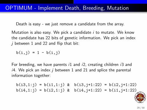
OPTIMUM - Implement Death, Breeding, Mutation
Death is easy - we just remove a candidate from the array.
Mutation is also easy. We pick a candidate i to mutate. We knowthe candidate has 22 bits of genetic information. We pick an indexj between 1 and 22 and flip that bit:
b(i,j) = 1 - b(i,j)
For breeding, we have parents i1 and i2, creating children i3 andi4. We pick an index j between 1 and 21 and splice the parentalinformation together:
b(i3,1:j) = b(i1,1:j) & b(i3,j+1:22) = b(i2,j+1:22)b(i4,1:j) = b(i2,1:j) & b(i4,j+1:22) = b(i1,j+1:22)
29 / 50
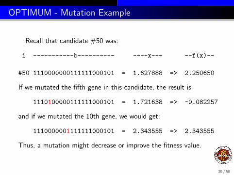
OPTIMUM - Mutation Example
Recall that candidate #50 was:
i -----------b---------- ----x--- --f(x)--
#50 1110000000111111000101 = 1.627888 => 2.250650
If we mutated the fifth gene in this candidate, the result is
1110100000111111000101 = 1.721638 => -0.082257
and if we mutated the 10th gene, we would get:
1110000001111111000101 = 2.343555 => 2.343555
Thus, a mutation might decrease or improve the fitness value.
30 / 50
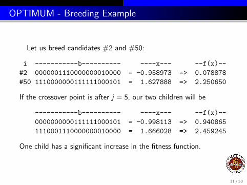
OPTIMUM - Breeding Example
Let us breed candidates #2 and #50:
i -----------b---------- ----x--- --f(x)--#2 0000001110000000010000 = -0.958973 => 0.078878#50 1110000000111111000101 = 1.627888 => 2.250650
If the crossover point is after j = 5, our two children will be
-----------b---------- ----x--- --f(x)--0000000000111111000101 = -0.998113 => 0.9408651110001110000000010000 = 1.666028 => 2.459245
One child has a significant increase in the fitness function.
31 / 50
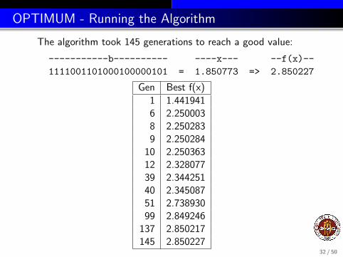
OPTIMUM - Running the Algorithm
The algorithm took 145 generations to reach a good value:
-----------b---------- ----x--- --f(x)--1111001101000100000101 = 1.850773 => 2.850227
Gen Best f(x)
1 1.4419416 2.2500038 2.2502839 2.250284
10 2.25036312 2.32807739 2.34425140 2.34508751 2.73893099 2.849246
137 2.850217145 2.850227
32 / 50
Genetic Algorithms
Introduction
Genetic Algorithms
A Simple Optimization
The Patchwork Picture
Conclusion
33 / 50
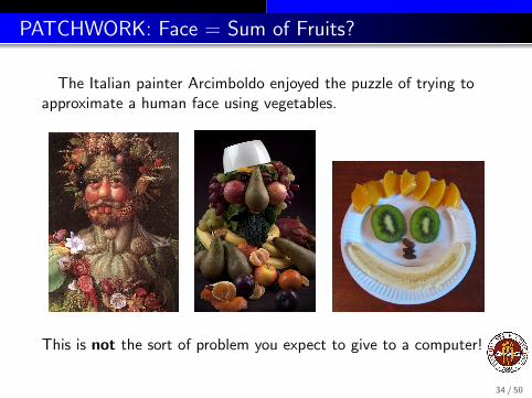
PATCHWORK: Face = Sum of Fruits?
The Italian painter Arcimboldo enjoyed the puzzle of trying toapproximate a human face using vegetables.
This is not the sort of problem you expect to give to a computer!
34 / 50
PATCHWORK: Face = Sum of Rectangles?
Nick Berry works for DataGenetics, and in his spare time, postsmany short, interesting articles about computing.
He read an article about genetic programming, but didn’t find thenumerical example very interesting; after thinking for a while, hecame up with a challenge that he wasn’t sure genetic programmingcould handle, and so he put some time into the investigation.
Could he teach his computer how to paint a picture of him?Instead of using fruit, he would add together 32 rectangles of color.
This problem is much more realistic and useful than trying tooptimize a function f (x). We’ll have to think about how to makeit fit into the genetic algorithm framework, and we already knowthat there’s no way that we can get a solution which is a perfectmatch for the original picture.
35 / 50
PATCHWORK - The Genetic Information
To make a genetic algorithm for this problem, we want to startby setting up the genetic information.
We assume the image is a jpg file containing 256× 256 pixels. Acandidate solution would be 32 colored rectangles. Each rectanglehas a position and a color. Using the jpg format, the lower leftcorner is a pair (xl , yl) between 0 and 255, and (xr , yr) is similar.The color of the rectangle is defined by three integers, r , g , and b,also between 0 and 255. Thus, our numeric representation of acandidate solution is 32 sets of (xl , yl , xr , yr , r , g , b), for a total of224 integers.
A number between 0 and 255 requires 8 bits to specify, so ourgenetic information describing one candidate would require224 ∗ 8 = 1792 bits.
36 / 50

PATCHWORK: One ”Gene”
We have 10 candidates or “chromosomes”. Each chromosomedescribes the color and position of 32 rectangles. The descriptionof a single rectangle is termed a “gene”.
37 / 50
PATCHWORK - The Fitness Function
Supposing we have specified a candidate solution x ; then wemust be prepared to evaluate its fitness f (x).
To evaluate our candidate, we can simply create a 256× 256 jpgfile from the rectangles, and sum the (r , g , b) color differencespixel by pixel:
f (x) =255∑i=0
255∑j=0
|r1(i , j)−r2(i , j)|+|g1(i , j)−g2(i , j)|+|b1(i , j)−b2(i , j)|
where r1 and r2 are the reds for original and candidate, and so on.
Note that a perfect solution would have f (x) = 0, and that lowvalues of f (x) are better than high ones. We remember that forthis problem, we are minimizing f (x) instead of maximizing.
38 / 50
PATCHWORK - The Fitness Function
The rest of the procedure is pretty straightforward. We have togenerate an initial random population of candidates, say 10 ofthem.
Our generation step will kill the 2 worst candidates, and replacethem by the two children produced by breeding the two bestcandidates. Then we will also pick one candidate at random andhit it with a random mutation.
A typical run of the program might involve thousands or hundredsof thousands of generations. To monitor the progress of theprogram, we can look at how the fitness function evaluations arechanging, or we can examine successive approximations to ourpicture.
39 / 50
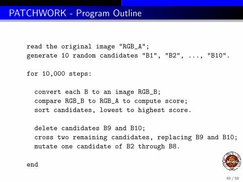
PATCHWORK - Program Outline
read the original image "RGB_A";generate 10 random candidates "B1", "B2", ..., "B10".
for 10,000 steps:
convert each B to an image RGB_B;compare RGB_B to RGB_A to compute score;sort candidates, lowest to highest score.
delete candidates B9 and B10;cross two remaining candidates, replacing B9 and B10;mutate one candidate of B2 through B8.
end
40 / 50
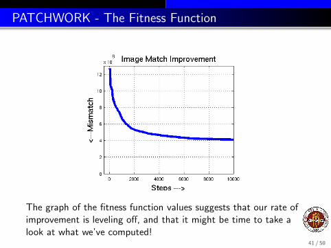
PATCHWORK - The Fitness Function
The graph of the fitness function values suggests that our rate ofimprovement is leveling off, and that it might be time to take alook at what we’ve computed!
41 / 50
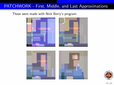
PATCHWORK - First, Middle, and Last Approximations
These were made with Nick Berry’s program.
42 / 50
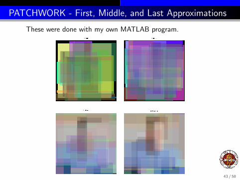
PATCHWORK - First, Middle, and Last Approximations
These were done with my own MATLAB program.
43 / 50
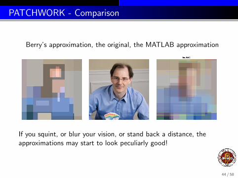
PATCHWORK - Comparison
Berry’s approximation, the original, the MATLAB approximation
If you squint, or blur your vision, or stand back a distance, theapproximations may start to look peculiarly good!
44 / 50
PATCHWORK - Color Combination
If you compare Nick Berry’s results to mine, they seem to be bydifferent “artists”. In particular, it’s easier to see the rectangleborders in Berry’s pictures.
This is because, I believe, Berry and I differ in how we combinedthe colors when two (or more) rectangles overlapped. He takes themaximum, and I take the average. Thus, rectangles with RGBcolors (50,100,150) and (250, 0, 100 ) would combine to
(250, 100, 150) in Berry’s method;
(150, 50, 125) in my method.
so Berry’s pictures are brighter and the boundaries betweenrectangles are sharper.
45 / 50
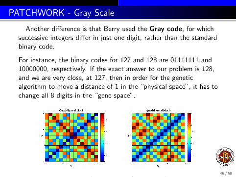
PATCHWORK - Gray Scale
Another difference is that Berry used the Gray code, for whichsuccessive integers differ in just one digit, rather than the standardbinary code.
For instance, the binary codes for 127 and 128 are 01111111 and10000000, respectively. If the exact answer to our problem is 128,and we are very close, at 127, then in order for the geneticalgorithm to move a distance of 1 in the “physical space”, it has tochange all 8 digits in the “gene space”.
Figure: Distance maps for binary and Gray codes, for 0 through 15.46 / 50

Genetic Algorithms
Introduction
Genetic Algorithms
A Simple Optimization
The Patchwork Picture
Conclusion
47 / 50
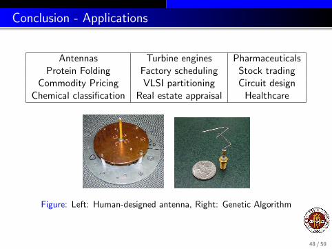
Conclusion - Applications
Antennas Turbine engines PharmaceuticalsProtein Folding Factory scheduling Stock trading
Commodity Pricing VLSI partitioning Circuit designChemical classification Real estate appraisal Healthcare
Figure: Left: Human-designed antenna, Right: Genetic Algorithm
48 / 50
Conclusion - Machine Learning
Genetic algorithms are an example of an exploding field incomputational science, known as machine learning.
Instead of trying to come up with instructions for solving aproblem, we can tell a computer what a solution looks like, let itlook at lots of examples, and come up with its own solutionmethods. (This is how spam filters work these days.)
We used to think that if you can’t understand how to solve aproblem, then you can’t solve the problem - but with geneticalgorithms, we can see that’s not always true.
One of the hardest problems we can imagine is how a life form cansurvive, outlive its rivals, and reproduce . . . and yet life has beenstumbling on better and better solutions for a billion years.
49 / 50
Conclusion - THANKS
I thank Professor Hoa Nguyen for the invitation to speak here!
50 / 50