GENDER BIAS IN SEX RATIO AT BIRTH: THE CASE OF INDIA

Rebeca A. Echávarri

D.T.2006/05

Gender Bias in Sex Ratio at Birth:

The Case of India∗.

Rebeca A. Echavarri†

Public University of Navarre and CSC (Cambridge University)

Keywords: Female Disadvantage, Autonomy to Act, Autonomy to Pre-fer, Capabilities, Asia, India.

JEL classification: J1, O53

Abstract

A deeply-rooted preference for sons may decrease the relativenumber of female births. Though there are variables that mayhelp to erode the couple’s preference for sons, these same vari-ables may also increase the availability of means to ensure malebirths. This is the case of educational achievements. It is notdifficult to assume, for example, that a higher level of educa-tion helps to erode the couple’s preference for sons. However,the effect of an increase in education on female disadvantage atbirth is not so straightforward. More education may increase thecouple’s awareness of the possibility of using prenatal sex detec-tion. We discuss the issue throughout the paper by developingan empirical framework for the case of India.

∗I am grateful to Jean Dreze for his encouragement in this research project. I also wishto thank Jorge Alcalde-Unzu, Miguel Angel Ballester, Roberto Ezcurra, Henrike Galarza,Reetika Khera and Jorge Nieto for reading an earlier draft of this paper, the Departmentof Geography of Delhi School of Economics, Delhi University, for their help in mappingsome of the results. I also wish to thank participants at the international conferences heldat CSC (Cambridge) and at Osaka University (Osaka). The project is supported by theSpanish Government (CICYT: SEC 2003-08105) and was developed during my stay at theCentre for Development Economics at the Delhi School of Economics, Delhi University(India).

†Public University of Navarra (Department of Economics), Campus de Arrosadia,31006, Pamplona (Spain). E-mail: rebeca.echavarri@unavarra.es; Phone: +34 948166021;Fax: +34 948169721.

1

1 Introduction.

A growing body of literature brings to light the issue of gender bias inmortality. By estimating the additional number of females of all ages thatwould be alive in the absence of gender inequality - and naming them the‘missing women’ - Amartya Sen (1990) calculates the cumulative impactof gender bias in mortality. In this way he shows how an alarmingly highnumber of women are missing as a consequence of gender inequality. As anexample, the missing women number over 100 million in South Asia, WestAsia, and North Africa (see Coale, 1991; Klasen and Wink, 2003, for somerefinements in these calculations).

Moreover, in a large part of the world, the number of missing women isincreasing dramatically. This situation is clearly illustrated by the downwardtrend in their sex ratio - the number of females divided by the number ofmales -. Studies of this downward trend have been carried out for severaldifferent countries, such as India (see Bhat, 2002a, 2002b; Dyson and Moore,1983; Mukerjee, 1976), China (see Junhong, 2001), Korea (see Kim, 2005),Bangladesh (see D’Sourza and Chen, 1980).

This paper is focuses on the case of India, and on the ‘sex ratio at birth(SRB)’. In India, the sex ratio of the total population has been steadilydecreasing since the last century, as reported in the appendix (figure 1).This is also the case of the sex ratio of the child population. We refer toMukherjee (1976) for an analysis of the downward trend of the first partof the century. The trend from 1961 to 2001 is displayed in the appendix(figure 2). All the results shown in the appendix are calculated from theprovisional 2001 census of India (Government of India, 2001).

A deep-rooted preference for males is thought to be the main reasonfor gender bias in the sex ratio, and the sex ratio at birth in particular(see Ben-Porath and Welch, 1976; Kim, 2005). Hence, the paper begins bypresenting, in section 2, the issue of the process by which parents developtheir preferences with respect to the sex of their unborn children. Theassumptions of the preference formation process are tested in section threeusing data from the 1991 Census of India at district level (Government ofIndia, 1991, 1997, 1998, 2003). The last section presents the conclusions.

2 Preferences and autonomy.

Before exploring the effects of preference for sons, we consider the notionof ‘autonomy to prefer’. This is seen as a person’s ability to develop thesame values that she would develop in a context where freedoms are fullyguaranteed. A couple may develop a preference for sons due to a historic

2

background of female disadvantage. These people are hardly able to attachthe same value to every human life, as would be the case in an alternativecontext of equality. People unconsciously suppress certain potential values.

The notion of autonomy to prefer - although connected - differs from thatof ‘autonomy to act’. Autonomy to act is related to a person’s fulfilment ofher preferences. This notion is very close to the general notion of ‘freedom ofchoice’ (see Pattanaik and Xu, 1990, and literature following their seminalwork). People’s achievements do not fully match their preferences whenthey lack the instruments that would enable them to act in accordance. Acouple with a preference for sons may not satisfy this preference (may havea daughter) if the technology that would enable them to ensure the sex oftheir future child is unavailable. Given an expansion of their freedom ofchoice, the couple would ensure the sex of their child. In other words, thecouple may gain in their autonomy to act without experiencing any variationin their autonomy to prefer.

In a context of substantial gender differences in the autonomy to act,virtually everybody is restricted in their autonomy to prefer. A growingbody of literature supports that autonomy to prefer is restricted to those whosuffer disadvantage. In order to avoid suffering from the inability to fulfil adesire, people may unintentionally suppress it. Elster (1982) uses Aesop’swell-known fable to illustrate the mental adaptation of humans (the processknown as ‘adaptive preference formation’). That is, when the fox realisesit is unable to reach the bunch of ripe grapes; it tells itself that they aresour. Nussbaum (2000) illustrates the case of women’s mental adaptation incontexts of gender inequality. In her words, a woman suffering disadvantagemay lose “the concept of herself as a person with rights”(Nussbaum 2000:113).

At the same time, the context of extreme gender inequality (of action)may also constrain autonomy to prefer for those who take advantage ofinequality. People are more likely to develop a preference for sons in this kindof context that in contexts where freedoms are fully guaranteed. Koopmans(1964) and Kreps (1979) put forward the idea of preference for flexibility.That is, when people’s present choices affect their future options, they preferwhatever current options will extend the set of future options. A child’s sexplays a significant role in defining the family’s future options in a context ofinequality (see Dyson and Moore, 1983; Srinivasan, 2005).

There are kinship structures (dowry system, women moving away fromtheir parents’ home at marriage) in which the daughters of the family entaila higher future cost than sons do. The dowry system, for example, consists

3

of the payment of revenue by families in order to have their daughters (nottheir sons) married. If they have to pay a dowry, an already poor family maybe pushed into dire poverty. Although this kinship structure is now illegalin India, dowry practices continue to survive. In a recent study of India,Srinivasan (2005) highlights the importance of dowry practices in definingthe family’s future options. Hence, the presence of a very deeply rootedpreference for males is a plausible assumption in our case study.

2.1 Effects of preference for sons.

A deeply rooted preference for males is thought as one of the main reasonsfor gender bias in mortality. Certainly, it is difficult to accept that parentsdeliberately act against their daughters. This perspective is maintained bythe Government of India (1981), among other authors. They insist on therebeing “little evidence to support the view that there is a deliberate neglectof female babies despite the fact that there may be a preference for malechildren”.

On the other hand, there exists evidence to show that sons are betterprovided for in the distribution of scarce resources than daughters are, atleast in dire living conditions (see Murthi, Guio and Dreze, 1995; Rosenzweigand Schultz, 1982; Sen and Sengupta, 1983). Sen and Sengupta (1983), forexample, find that the enhancement of general living conditions barely en-larges the capabilities of girls in times of disaster. They set their frameworkin two villages in West Bengal. These villages were selected because one ofthem had undergone land reform, while the other had not. Land propertytends to be decentralised after reform, which leads to the enhancement ofaverage family living conditions. After conducting a nutritional survey onchildren up to five, they conclude the following: while malnutrition is highin both villages, it is in fact higher in the one that has not undergone landreform. Moreover, it is also the case that improvements in child nutritionpatterns are associated with higher gender inequality. While general im-provements enhance nutrition patterns in boys, they hardly do so at all inthe case of girls.

Another context in which to examine the (possible) satisfaction of thepreference for sons is at birth. In societies in which sex selection is notpractised, the distribution of SRB is relatively constant for the country asa whole. This was the assumption reached in some general studies on de-mographic outcomes, such as Becker (1960) and Trivers and Willard (1973).Later on, advances in prenatal sex determination transformed the scenario.The expansion of prenatal sex determination now enables families to choosethe sex of their new child by practising abortion when the foetus is not of thedesired sex. When sex preferences matter, some biases arise in the reportedSRB, as in the case of India.

4

Instead of a relatively constant overall distribution of SRB, certain pat-terns emerge. The estimated SRB in areas of north-west India is lower thanin the rest of India, as illustrated by the maps that appear in the appendix(figures 3 and 4). Maps in figures 3 and 4 correspond to urban and ruralareas, respectively. Data from the 1991 Census of India are used in theestimates.

Although the 1991 Census of India does not provide SRB data at districtlevel, it is possible to calculate it from the data actually released. The Gov-ernment of India (1991), in the Primary Census Abstract (PCA) for 1991,supplies the available data for the population aged 0-6 by gender. Further-more, the Government of India (1997) uses data from the 1991 census toestimate child mortality by gender at different ages. Estimates are based onthe South Asian model life and modified via the Brass procedure. Partiallyguided by that report, we estimate SRB using a reverse survival technique.Similar estimates of sex ratio at birth are provided in Bhat (2002b) andSudha and Irudaya Rajan (1998). Our calculations are displayed in theappendix (Calculations 1).

All in all, comparing figures 3 and 4, the basic patterns are largelysimilar. They portray higher female disadvantage for districts in North-west India, which is consistent with earlier studies. For example, Dysonand Moore (1983) identifies northern and western districts (in Gujarat, Hy-machal Pradesh, Rajasthan, Uttar Pradesh, Madhya Pradesh, Punjab andHaryana) as registering high gender bias in mortality.

At the same time, we notice that fewer women are born in urban areasthan in rural ones. Certainly, urban areas currently have better access tomodern medical techniques. Since Sudha and Rajan (1998) documented anexpansion in the availability and use of prenatal sex determination and abor-tion technology in rural areas, the patterns in rural areas may be strength-ened. This would occur under continuing extreme gender inequality, andhence, persistent preference for sons. In any case, the existence of patternsshowing bias in mortality at birth makes us aware that son preference existsand put into practice.

In the next section we develop an empirical framework where we test therelationship between gender differences in terms of autonomy to act and biasin SRB. As discussed, it is expected that preference for sons is very deeplyrooted in those districts where gender differences in autonomy to act aregreater. Hence, we will hardly be surprised to find a negative relationshipbetween the degree of inequality (in terms of autonomy to act) and thenumber of female births (conditional to the number of male births).

At the same time, we test to see how enlarging autonomy to act affectsbias in SRB. In this case, the increment in autonomy to act is expected to

5

decrease SRB in those districts where there is a very deeply rooted prefer-ence for sons. However, we expect the opposite effect from an incrementin autonomy to prefer. An increment in autonomy to prefer is expected toerode preference for sons and then increase SRB.

3 An empirical framework.

Proceeding with this research, we now test the relationship between inequal-ity in terms of autonomy to act and gender bias in mortality. At the riskof oversimplifying the issue, and for identification purposes, we assume thisrelationship to be linear. For modelling purposes, first consider the followingnotation,

i the district,

SRBi the number of female births divided by the number of malebirths in i,

Xi the vector of variables describing gender differences in auton-omy to act in i,

Yi the vector of variables capturing the degree in autonomy toact in i.

Then, we specify the relationships among variables by using a linearregression model as follows,

SRBi = β0 + Xiβ1 + Yiβ2 + εi (1)

where εi is the random disturbance.

Throughout the section we estimate the coefficients of the regression.Moreover, we regress two versions of the econometric model displayed inequation 1, one a reduced model, the other an extended model. In the re-duced form, a measure of gender differences in access to ‘independent incomeopportunities (IIOD)’ is used as proxy for gender differences in autonomy toact. In this model, an ‘index of the wealth of the region (W)’ is also addedas proxy for district-varying explanatory features capturing autonomy toact. Indeed, wealth helps individuals to match desires and achievements.Formally, the reduced model is written as:

SRBi = β′

0 + β′

1IIODi + β′

2Wi + ε′

i (2)

The extended model also accounts for the effect of ‘educational achieve-ments (E)’ in the district, for the effect of variables referred to the ‘presence

6

of scheduled castes (SC)’, and for the effect of access to ‘medical services(MS)’. Formally,

The extended model is written as:

SRBi = β′′

0 + β′′

1 IIODi + β′′

2 Wi + β′′

3 Ei + β′′

4 SCi + β′′

5 MSi + ε′′

i (3)

Medical services are used as proxy for services that could enable people touse sex-selective abortion technology, while the presence of scheduled castesindicates the proportion of people with higher access to such facilities. Morecomments are required for the role of education on explaining bias in SRB.The role of education in explaining bias in SRB requires further comment,because education captures not only a person’s degree of autonomy to prefer,but also her autonomy to act.

On the one hand, education increases a person’s autonomy to act. ThePlanning Commission for India (in the introduction of the 10th Five-YearPlan 2002-2007) highlights the importance of education to raise awarenessof opportunities. It is recognised that the lack of education among poorpeople constitutes one of the main obstacles to their making use of incomegrowth, for example. In the same way, lack of education may be a majorimpediment preventing individuals from making use of, say, sex-selectiveabortion technology.

On the other hand, education increases a person’s degree of autonomyto prefer. Education provides individuals with human skills needed for in-dependence of mind, such as reasoning and judging. It is worth noting thata large body of literature provides evidence to support the fact that incre-ments in education erode preference for males. To give an example, Bhatand Zavier (2003) infer that education reduces son preference after estimat-ing a multivariate regression model based on data from the Indian NationalFamily Health Survey. The theory that daughters receive a greater shareof household resources when women’s opportunities are greater also findssupport in the empirical results of Murthi et al. (1995).

Hence, the effect captured by parameter β′′

3 accounts for the effect ofeducation on autonomy to act - and autonomy to act on SRB - and forthe effect of education on autonomy to prefer - and autonomy to prefer onSRB. Once again, there are powerful reasons to believe that these two effectswork in opposite directions. While an increment in autonomy to prefer isexpected to erode preference for sons and then increase SRB, an incrementof autonomy to act is expected to decrease SRB in the presence of preferencefor sons.

7

All in all, as noted earlier, the key issue of identification concerns therelationship between gender differences in terms of autonomy to act andgender bias in SRB. The relationship is captured by parameter β1 in equation1. This is done by parameters β

′

1 and β′′

1 in equations 2 and 3, respectively.The positive sign of the parameter identifies a negative relationship betweenthe degree of gender differences in autonomy to act and the number of femalebirths (conditional to the number of male births).

3.1 Data set and sample

The data set at district level is compiled from reports based on Indian Cen-suses, and referred to year 1991 (Government of India 1991, 1998, 2003).This releases information of educational achievements, labour opportuni-ties, and other specific information about availability of resources in thedistricts (such as access to medical services) or other demographic features(such as the distribution of social groups).

At the same time, we focus on a sample of 333 districts for which therequired information is available. Some features of the sample are listed inwhat follows. According to demographic studies, the expected SRB is about950 female births per 1.000 male births (see Johansson and Nygren, 1991;Visaria 1971, among others). In 173 out of the 333 districts in the sample,the SRB takes values below .950. Furthermore, one hundred districts takevalues below .935. That is, a large number of the districts in the sampledisplay gender bias in their reported SRB.

As far as the features of the population in the sample are concerned, 28percent of the whole population are reported as having independent incomeopportunities, 89 percent of them are males. Regarding the educationalachievements, education is extended to sixty percent of the population.Males account for sixty percent of educated people. Furthermore, in allof the districts, both the number of educated males to the total of malepopulation and the number of males having independent income opportuni-ties to the total of male population surpass the corresponding numbers forfemales.

3.2 Definition of the variables

As already noted, our dependent variable - the SRB - is estimated using areverse survival technique based on the South Asian model life and mod-ified via the Brass procedure. Calculations are made from the 1991 data(Government of India 1991, 1997). Our calculations are displayed in theappendix (Calculations 1).

The index for gender differences in access to independent income oppor-tunities is defined by the difference between the ratio of female main workers

8

to the total female population minus the same ratio for males. The calcula-tions are based on data from Government of India (1991). Main workers aredefined in the census as those engaged in paid employment for a minimumof 183 days a year. Unpaid employment, such as slavery, is not consideredto be main work. Hence, the main worker variable can be considered anadequate approximation of independent income opportunities.

In order to capture district wealth, we use the wealth index, definedon the interval [0,1], and drawn from Government of India (2003). Theircalculations are based on the data from the 50th round of National SampleSurvey Organisation’s survey on household expenditure and income. Ourmain reason for using this wealth index is that, as far as we are aware, for1991 at least, the Government of India has released no standard index data,such as GDP, at the district level.

As far as educational achievements are concerned, we focus on literacystandards. For societies with universal literacy, education is better repre-sented by an elaborated educational index, such as the measure of progresstoward universal primary education. As noted earlier, however, this is thecase of our sample. Therefore, the literacy rate is an adequate proxy foreducational achievements in our case study. Furthermore, literacy rates arecalculated as the ratio of literate population to the total population. Thecalculations are based on data from Government of India (1991), where aperson is assumed to be literate if she is aged seven years or more and canboth read and write with understanding in any language.

In the case of other districts level data, it is worth noting the following.The ratio of the scheduled castes to the total population is compiled fromGovernment of India (1991), where no-one professing a religion other thanHinduism, Sikhism or Buddhism is deemed to belong to scheduled castes.Regarding access to medical services, data on the proportion of villages withsome form of medical facility is compiled from Government of India (1998).Basic statistics of these variables are displayed in the appendix (table 1).

3.3 Econometric methodology

The estimation of the parameters in the reduced and extended models (equa-tion 2 and equation 3) raises some econometric issues. The Ordinary LeastSquares (OLS) method provides efficient estimates of parameters when dis-turbances are normally distributed. The normality assumption is violated,however, because no relationship among variables is captured in the courseof the regression. In our study case, there are reasons to suspect that gen-der bias in mortality is strongly associated with geographical location. Onearlier maps, geographically adjacent values tend to be similar.

9

There are several different procedures to cope with spatial correlationbias. One of them consists in introducing dummy variables for each State.Such a model is estimated by the OLS method. When the model includesa large dummy variable set, an alternative method is to define a categoricalvariable and estimate the model by a fixed-effects method. We estimate thereduced and extended models using State as the categorical method. TheOLS and fixed-effects estimates are displayed in the appendix (table 2).

At the same time, spatial dependence can also be captured by including avariable created by combining the SRB vector and a geographic connectivitymatrix. Elements of the matrix capture spatial dependence among districts.The variable is named ‘spatially lagged SRB (SLSRB)’ throughout the pa-per because its corresponding parameter in the ordinary regression capturesspatially-lagged SRB (see Berik and Bilginsoy, 2005). Following this proce-dure, the OLS estimates of the reduced and extended models are displayedin the appendix (table 2, columns 3 and 6).

Violation of the normality assumption may also be due to heteroskedas-ticity. Disturbances are heteroskedastic when they have different variances.To check disturbances for heteroskedasticity, we apply White’s general test,the results of which are shown in the appendix (table 2). The hypothesis ofhomoskedasticity cannot be rejected on the basis of these results.

Before estimating the parameters of the regression model, the sampleis checked for outliers by applying Hadi’s method to measure the distancefrom each observation to a cluster of points. This identifies Nellore, oneof the districts in Andhara Pradesh, as the only outlier. Removal of thisdistrict from our sample does not alter the parameter values, though theirsignificance is strengthened. At the same time, for a more complete test ofrobustness, we compare the coefficients of the reduced and extended models.This comparison yields no variation in the sign and significance of the keyparameters. Furthermore, there is no statistical variation in the dimensionof the parameters. Hence, our results can be considered robust.

3.4 Main econometric results.

As formerly noted, we are interested in estimating the sign of the relationshipbetween autonomy to act and gender bias in SRB, identified by parameterβ1. We refer comments to parameter β1, rather than to parameters β

′

1

and β′′

1 separately, because there are no statistical differences between theirestimates. Furthermore, there are no statistical differences in sign, size andsignificance between OLS estimates and fixed-effect estimates.

All the estimates of parameter parameter β1 are significantly differentfrom zero, taking values that are above zero. The result shows a negative

10

relationship between gender inequality (in terms of autonomy to act) andthe number of female births (conditional to the number of male births).In particular, preference for sons appears to be strengthened by gender in-equality in autonomy to act. Fewer female births occur in areas with scarcerindependent income opportunities for females. Our result is consistent withstudies on the relationship between females’ labour opportunities and childsurvival bias (see Berik and Bilginsoy, 2005; Rosenzweig and Schultz, 1982,among others).

At the same time, we examine the effect of the degree of autonomy toact in an attempt to explain bias in the SRB. Inter district variations inautonomy to act across districts are captured in the model by variables suchas district wealth. The negative value of estimates capturing the effect ofwealth in explaining bias in SRB reveals a negative relationship betweenwealth and the number of female births. The result is corroborated in theextended model.

As far as education concerns, it is worth noting the following. Theestimates shows a negative relationship between educational achievementsand SRB. The result evidences that the decline in female births due toawareness of new technology is greater than the increment in female birthscaused by a weakening of son preference. This strengthens our belief ofthere being a very deep-rooted preference for sons, which counteracts the(possible) positive effect of education on female survival.

An additional point of interest is the study of the effect of the enhance-ment of mothers’ living conditions, especially as far as maternal health isconcerned. Improvements in maternal health not only reduce maternalmortality, but also reduce the probability of an additional child dying atbirth. Human Geography generally assumes that the probability of death atbirth is higher in males than in females, therefore improvements in maternalhealth may raise the proportion of male births (see Bhat, 2002b; Trivers andWillard, 1973, among others). This may be used to justify the reductionin the SRB. However, it is hardly possible that (in the absence of genderbias at birth) increased maternal health brings SRB below 950 female births(per 1,000 male births). This is in fact the commonly accepted ratio in theabsence of female disadvantage (see Visaria, 1971).

Finally, geography is fundamental as evidenced by the statistical signifi-cance of the parameters associated with the regional dummy variables. Theclose relationship among districts within the same State may conceivablybe due to cultural features and factors relating to the expansion of rights(see Dyson and Moore, 1983). However, data to capture these features atdistrict level are not available at present.

11

4 A remark.

Throughout the paper, we examine the effect of preference for sons on the re-lation of female births to male births. We prove that increasing women’s op-portunities (conditional to men’s opportunities) increases the relative num-ber of female births. Furthermore, we guess that female disadvantage willdecrease as people gain more autonomy to prefer. Analysis of the centralissue of autonomy to prefer will be facilitated by the availability of gender-desegregated data on the guarantee of entitlement over resources and rights,for instance. At present, we can only test our hypothesis against the expe-rience of those regions of the world where raising a son or a daughter makeslittle difference to the family’s future options. It is quite interesting to notethat, currently, more girls (per 1.000 boys) are born in those regions of theworld where a child’s sex is not a strong determinant of the family’s futureoptions than in those societies where it has a determining effect.

References

[1] Becker, Gary S. 1960. An Economic Analysis of Fertility. Reprinted in TheEconomic Approach to Human Behavior, Gary S. Becker. 1976. Chicago: TheUniversity of Chicago Press.

[2] Berik, Gunseli, and Cihan Bilginsoy. 2000. ‘Type of Work Matters: Women’sLabor Force Participation and the Child Sex Ratio in Turkey.’ World Devel-opment 28(5): 861-78.

[3] Bhat, Mari P.N. 2002a. ‘On the Trail of Missing Indian Females. I: Search forClues.’ Economic and Political Weekly 21: 5105-18.

[4] Bhat, Mari P.N. 2002b. ‘On the Trail of Missing Indian Females. II: Illusionand Reality.’ Economic and Political Weekly 21: 5244-63.

[5] Bhat, Mari P.N., and Francis AJ Zavier. 2003. ‘Fertility Decline and GenderBias in Northern India.’ Demography. 40(4): 637-57.

[6] Ben-Porath, Yoram, and Finis Welch. 1976. ‘Do Sex Preferences Really Mat-ter?’ Quarterly Journal of Economics 90(May): 285-321.

[7] Coale, Ansley J. 1991. ‘Excess Female Mortality and the Balance of the Sexes inthe Population: an Estimate of the Number of ‘Missing Females’.’ Populationand Development Review 17: 517-23.

[8] D’Sourza, Stan, and Lincoln C. Chen. 1980. ‘Sex Differences in Mortality inRural Bangladesh.’ Population and Development Review 6: 257-20.

[9] Dyson, Tim, and Mick Moore. 1983. ‘On Kinship Structure, Female Autonomy,and Demographic Behavior in India.’ Population and Development Review 9:35-60.

[10] Elster, John. 1982. ‘Sour Grapes-Utilitarianism and the Genesis of Wants.In Utilitarianism and beyond, eds. Amartya K. Sen, and Bernard Williams.London: Cambridge University Press.

12

[11] Government of India. 1981. ‘Provisional Population Totals of 1981.’ 1981 IndiaCensus (Series 1, India, Paper N. 1). New Delhi: Office of the Registrar Generalof India.

[12] Government of India. 1991. ‘Primary Census Abstract (PCA) of 1991.’ 1991India Census (District Level). New Delhi: Office of the Registrar General.

[13] Government of India. 1997. ‘District Level Estimates of Fertility and ChildMortality for 1991 and their Interrelations with Other Variables.’ 1991 IndiaCensus (Occasional Paper N. 1 of 1997). New Delhi: Office of the RegistrarGeneral.

[14] Government of India. 1998. ‘Availability of Infrastructural Facilities in RuralAreas of India: An Analysis of Village Directory Data.’ 1991 India Census.New Delhi: Office of the Registrar General.

[15] Government of India. 2001. ‘Provisional Population Totals.’ 2001 India Cen-sus (Series 1, India, Paper N. 1 of 2001). New Delhi: Office of the RegistrarGeneral.

[16] Government of India. 2003. ‘Report of the Task Force: Identification of Dis-tricts for Wage and Self Employment Programmes.’ New Delhi: Planning Com-mission of India.

[17] Johansson, Sten, and Ola Nygren. 1991. ‘The Missing Girls of China - A NewDemographic Account.’ Population and Development Review 17: 35-51.

[18] Junhong, Chu. 2001. ‘Prenatal Sex Determination and Sex-Selective Abortionin Rural Central China Population and Development Review 27: 259-81.

[19] Kim, Jinyoung. 2005. ‘Sex Selection and Fertility in a Dynamic Model of Con-ception and Abortion.’ Journal of Population Economics 18: 41-67.

[20] Klasen, Stephan, and Claudia Wink. 2003. ‘Missing Women: Revisiting theDebate.’ Feminist Economics 9: 263-99.

[21] Koopmans, Tjalling C. 1964. ‘On Flexibility of Future Preference.’ In HumanJudgments and Optimality, eds., Maynard W. Shelley, and Glenn L. Bryans.New York John Wiley and Sons Inc.

[22] Kreps, David M. 1979. ‘A Representation Theorem for ‘Preference for Flexi-bility’.’ Econometrica 47: 565-78.

[23] Mukherjee, Sudhansu B. 1976. ‘The Age Distribution of the Indian Population.A Reconstruction for the States and Territories, 1881-1961.’ Honolulu: East-West Population Institute.

[24] Murthi, Murthi, Anne C. Guio, and Jean Dreze. 1995. ‘Mortality, Fertility andGender Bias in India: A District-Level Analysis.’ Population and DevelopmentReview 21.

[25] Nussbaum, Martha C. 2000. Women and Human Development: the Capabili-ties Approach. Cambridge: Cambridge University Press.

[26] Pattanaik, Prasantta K, and Yongsheng Xu. 1990. ‘On Ranking OpportunitySets in Terms of Freedom of Choice.’ Recherches Economiques de Louvain 56:383-90.

13

[27] Rosenzweig, Mark, and Paul T. Schultz. 1982. ‘Market Opportunities GeneticEndowments and Intrafamily Resource Distribution: Child Survival in RuralIndia.’ American Economic Review 72(4):803-15.

[28] Sen, Amartya K. 1990. ‘More than 100 Million Women are Missing.’ The NewYork Review of Books 20 (December).

[29] Sen, Amartya K., Sunil Sengupta. 1983. ‘Malnutrition of Rural Children andthe Sex Bias.’ Economic and Political Weekly 19 (annual number).

[30] Srinivasan, Sharada. 2004. ‘Daughters or Dowries? The Changing Nature ofDowry Practices in South India.’ World Development 33(4):593-615.

[31] Sudha, Shreeniwas, and S Irudaya Rajan. 1998. ‘Intensifying Masculinity ofSex Ratios in India: New Evidence 1981-1991.’ Thiruvananthapuram: Centrefor Development Studies.

[32] Trivers, Robert L., and Dan E. Willard. 1973. ‘Natural Selection of ParentalAbility to Vary the Sex Ratio of Offspring.’ Science 179(4068): 90-92.

[33] Visaria, Pravin. 1971. ‘The Sex Ratio of the Population of India.’ 1971 IndiaCensus (Paper N. 10). Delhi: Manager of Publications.

14

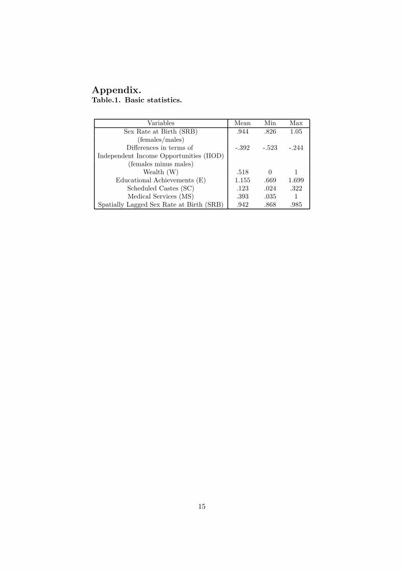
Appendix.Table.1. Basic statistics.

Variables Mean Min Max

Sex Rate at Birth (SRB) .944 .826 1.05(females/males)

Differences in terms of -.392 -.523 -.244Independent Income Opportunities (IIOD)

(females minus males)Wealth (W) .518 0 1

Educational Achievements (E) 1.155 .669 1.699Scheduled Castes (SC) .123 .024 .322Medical Services (MS) .393 .035 1

Spatially Lagged Sex Rate at Birth (SRB) .942 .868 .985

15

Table.2. Basic Results of a Cross-section Analysis of the De-terminants of Sex Rate at Birth (SRB) in Urban Indian Districts(1991).

IndependentVariables

1 2 3 4 5 6

————– ————– ————– ————– ————– ————–IIPD .079 .079 .051 .085 .085 .058

(.029)** (.029)** (.021)* (.030)** (.030)** (.021)**W -.019 -.019 -.012 -.020 -.020 -.012

(.007)** (.007)** (.005)* (.007)** (.007)** (.005)*E -.018 -.018 -.009

(.009)* (.009)* (.005)SC -.059 -.059 -.056

(.027)* (.027)* (.023)*MS -.013 -.013 -.003

(.006)* (.006)* (.003)constant .921 .985 1.000 .964 .997 .173

(.013)** (.011)** (.059) (.022)** (.015)** (.066)**

SLSRB .923 .868(.058)** (.064)**

F-test(P-value) .0000 .0008 .0000 .0000 .0003 .0000White(P-value) .915 .49 .996 .98

R sq .57 .57 .56 .59 .59 .58Sample size 333 333 333 333 333 333

Notes:1: SRB reduced model estimated by OLS method.2: SRB reduced model estimated by fix effect method.3: SRB reduced model estimated by OLS method.4: SRB extended model estimated by OLS method.5: SRB extended model estimated by fix effect method.6: SRB extended model estimated by OLS method.1 and 4: Includes country dummies, but not reported. Almost all of them are statis-

tically significant at .01 level.

Robust standard errors in brackets.**Significant at .01 percent level. * Significant at .05 percent level.

16

Figure Legends

Figure 1.: Sex Ratio of total population is calculated as the ratio of femalepopulation to male population.

Figure 2.: Sex Ratio of total population is calculated as the ratio of femalepopulation to male population. Sex Ratio of child population is calculatedas the ratio of female population in age group 0-6 to male population in agegroup 0-6.

Figure 3.: Values are labeled as follows: Female Advantage if values ofestimated SRB are higher than 950 female born per 1,000 male born; andFemale Disadvantage if values are lower than this. Beyond this, we considerFemale Advantage to be high if this figure is above 970 and Female Disad-vantage to be high if the figure is below 935. Values for the divisions comefrom Visaria (1971)’s study of the common values assumed in demographicstudies.

Figure 4.: Values are labelled as follows: Female Advantage if values ofestimated SRB are higher than 950 female born per 1,000 male born; andFemale Disadvantage if values are lower than this. Beyond this, we considerFemale Advantage to be high if this figure is above 970 and Female Disad-vantage to be high if the figure is below 935. Values for the divisions comefrom Visaria (1971)’s study of the common values assumed in demographicstudies.

17

Figure 1.:

Source: Government of India (2001).

18

Figure 2.:

Source: Government of India (2001).

19

Figure 3.: Estimated Female Disadvantage at Birth, (Urban),1991 1

��������� � � ��� ������� �

�������� ���� �� ��������� � ����� �!��" �$# ��%$ # � &('�������� ���� �� ��������� � ����)!*+ �&�������� ���� �� ��������� � ����)�,���-�������� ������������� ������)�,���-�������� ������������� ������)!*+ �&

Source: Own elaboration from the data given in the PCA of 1991 Census of India.

1Values are labelled as follows: Female Advantage if values of estimated SRB are higherthan 950 female born per 1,000 male born; and Female Disadvantage if values are lowerthan this. Beyond this, we consider Female Advantage to be high if this figure is above970 and Female Disadvantage to be high if the figure is below 935. Values for the divisionscome from Visaria (1971)’s study of the common values assumed in demographic studies.

20

Figure 4.: Estimated Female Disadvantage at Birth, (Rural),19912

���������� ���� ������ �

�� ����� ��� ������������� ���� ����� � �"! $#" ! � %�&�' ����� ��� ������������� ���� �(�)� ��%�' ����� ��� ������������� ���� �(�*'��+�' ����� ,����������� ���� '(�*'��+�' ����� ,����������� ���� '(�)� ��%

Source: Own elaboration from the data given in the PCA of 1991 Census of India.

2See figure 2 for an explanation of the value labels.

21

Calculations 1

First, consider the next notation and definitions,

Fi the total of female survivors to recorded female births i yearsago,

Mi denotes total male survivors to recorded male births i yearsago,

qfk the probability of dying from birth to the age k for females

and, hence, qfk+1

is the probability of dying from birth to the endof the considered period,

qmk this probability for males,

Bf the annual average of female births,

Bm the same average for males,

Definition 1:The SR of child population in the age group (0-6), denoted SR(0-6), is

given by,

SR(0 − 6) =F0 + F1 + F2 + F3 + F4 + F5 + F6

M0 + M1 + M2 + M3 + M4 + M5 + M6

(4)

The ratio is based on the fact that population in the 0-6 age-group are thesurvivors from the births recorded during the current and the last six years.

Definition 2:The SR at birth, denoted SRB, is given by,

SRB =Bf

Bm(5)

This is the number of recorded female births divided by the number ofrecorded male births.

Our calculations to estimate the SRB from data released by Governmentof India (1991) are derived as follows. The survivors of female births recordedi years ago are expressed as,

Fi = Bf− Bfq

fi+1

= Bf (1 − qfi+1

) (6)

In the same way, the survivors of male births recorded i years ago aregiven by,

Mi = Bm− Bmqm

i+1 = Bm(1 − qmi+1) (7)

22

Then, the sex ratio of equation 1 can be expressed as a sum of thesurvivors of the births recorded during the current and the last six years.Formally,

SR(0 − 6) =Bf [(7 −

∑i=6

i=0qfi+1

)]

Bm[(7 −

∑i=6

i=0qmi+1

)](8)

From equations (2) and (5), we obtain the estimator of SRB as,

SRB = SR(0 − 6)7 −

∑i=6

i=0qmi+1

7 −

∑i=6

i=0qfi+1

(9)

For the calculations it is worth noting the next. The Government ofIndia (1997) only releases q1, q2, q3, q5, separately for females and males.For simplicity, we assume that mortality ratios are the same at ages threeand four and at ages five, six and seven. However, alternative interpolationsoffer similar results.

23