gaseous pollutant monitoring standard operating procedure ... · gaseous pollutant monitoring...

Gaseous Pollutant Monitoring Standard Operating Procedure (SO2, NOx, NOy, CO)

August 2017 Publication no. 17-02-009

Publication and Contact Information This report is available on the Department of Ecology’s website at https://fortress.wa.gov/ecy/publications/SummaryPages/1702009.html For more information, contact:

Jill Schulte | Anna Tai | Scott Dubble Air Quality Program P.O. Box 47600 Olympia, WA 98504-7600 (360) 407-6800

Washington State Department of Ecology - www.ecology.wa.gov

o Headquarters, Olympia 360-407-6000

o Northwest Regional Office, Bellevue 425-649-7000

o Southwest Regional Office, Olympia 360-407-6300

o Central Regional Office, Yakima 509-575-2490

o Eastern Regional Office, Spokane 509-329-3400

To request ADA accommodation, call Ecology at (360) 407-6800, 711 (relay service), or 877-833-6341 (TTY).

http://www.ecologyy.wa.gov/

Gaseous Pollutant (Sulfur Dioxide, Nitrogen Oxides, and Carbon Monoxide)

Monitoring Standard Operating Procedure

August 2017

Approved by: Signature: Date: Kathy Taylor, Deputy Air Quality Program Manager Signature:

Date:

Cullen Stephenson, Technical Services Section Manager Signature:

Date:

Mike Ragan, Air Monitoring Coordinator Signature:

Date:

Sean Lundblad, Quality Assurance Coordinator Signatures are not available on the internet version.

This page is purposely left blank

i

Table of Contents Index of Tables ............................................................................................................ ii Index of Figures........................................................................................................... ii Definitions and Acronyms.......................................................................................... iv

Chapter 1. Overview .........................................................................................................1

1.1. Purpose and Scope......................................................................................1 1.2. Data Quality Objectives .............................................................................2 1.3. Health and Safety .......................................................................................2

Chapter 2. Dilution Calibrator...........................................................................................4

2.1. Introduction ................................................................................................4 2.2. Principles of Operation...............................................................................4 2.3. Equipment and Supplies .............................................................................5 2.4. Installation Procedure .................................................................................6 2.5. Quality Control and Maintenance Procedure ...........................................10 2.6. Data Collection and Storage .....................................................................18 2.7. Data Validation and Quality Assurance ...................................................21

Chapter 3. Sulfur Dioxide (SO2) Monitoring ..................................................................22

3.1. Introduction ..............................................................................................22 3.2. Principles of Operation.............................................................................22 3.3. Equipment and Supplies ...........................................................................22 3.4. Installation ................................................................................................22 3.5. Quality Control and Maintenance ............................................................23 3.6. Data Collection and Storage .....................................................................29

Chapter 4. Nitrogen Oxides (NOx) and Reactive Nitrogen (NOy) Monitoring ..........36


Chapter 5. Carbon Monoxide (CO) Monitoring ...........................................................69


References ..........................................................................................................................83

ii

Table 1-1. Supported analyzers and required calibration equipment.............................................. 1 Table 2-1. Summary of gaseous pollutant standard hardware, tools, routine parts and supplies. .. 5 Table 2-2. Ecology and EPA quality control check terms ............................................................ 10 Table 2-3. Minimum required and recommended quality control check frequencies. ................. 10 Table 2-4. QC check acceptance criteria ...................................................................................... 13 Table 2-5. Summary of required dynamic dilution calibrator maintenance ................................. 16 Table 2-6. Summary of dilution calibrator diagnostic data .......................................................... 16 Table 3-1. Summary of required SO2 analyzer maintenance ........................................................ 24 Table 3-2. Teledyne API T100 and T100U diagnostic data (Teledyne API 2016) ...................... 27 Table 4-1. Summary of NO/NO2/NOx/NOy siting criteria............................................................ 37 Table 4-2. Summary of required NOx/NOy analyzer maintenance ............................................... 39 Table 4-3. Teledyne API M200EU diagnostic data (Teledyne API 2010) ................................... 43 Table 5-1. Summary of CO siting criteria..................................................................................... 70 Table 5-2. Summary of required CO analyzer maintenance......................................................... 71 Table 5-3. Teledyne API T300 and T300U diagnostic data (Teledyne API 2012) ...................... 74

Figure 2-1. Configuration of station probes and instruments (photos from Teledyne API). .......... 8 Figure 2-2. Example solenoid array for multiple gas analyzers (photo by Odelle Hadley) ........... 9 Figure 2-3. Selection of QC concentration points......................................................................... 12 Figure 2-4. Example of triggering QC check manually from Envidas Ultimate .......................... 14 Figure 2-5. Example ACTCONC channel configuration.............................................................. 19 Figure 2-6. Configuration of dilution calibrator diagnostic parameter collection. ....................... 20 Figure 3-1. SO2 action levels for recalibration ............................................................................. 23 Figure 3-2. Particulate filter assembly (Teledyne API 2016). ...................................................... 25 Figure 3-3. Timebase setting for collecting 5-minute average SO2 concentrations...................... 29 Figure 3-4. SO2 channel configuration ......................................................................................... 30 Figure 3-5. SO2 primary QC sequence properties......................................................................... 31 Figure 3-6. SO2 primary QC sequence configuration ................................................................... 32 Figure 3-7. SO2 primary QC configuration of validation limits ................................................... 33 Figure 3-8. SO2 primary QC configuration of phases and reference values ................................. 34 Figure 3-9. Configuration of SO2 analyzer diagnostic parameter collection ................................ 35 Figure 4-1. NO/NO2/NOx/NOy action levels for recalibration ..................................................... 38 Figure 4-2. Particulate filter assembly (Teledyne API 2016). ...................................................... 41 Figure 4-3. NO channel configuration. ......................................................................................... 46 Figure 4-4. NO2 channel configuration. ........................................................................................ 47 Figure 4-5. NOx channel configuration. ........................................................................................ 48

iii

Figure 4-6. NO/NO2/NOx primary QC sequence properties configuration. ................................. 50 Figure 4-7. NO/NO2/NOx primary QC sequence part 1................................................................ 51 Figure 4-8. NO/NO2/NOx primary QC sequence configuration part 2. ........................................ 52 Figure 4-9. NO/NO2/NOx primary QC validation limits configuration. ....................................... 53 Figure 4-10. NO primary QC configuration of phases and reference values. .............................. 54 Figure 4-11. NO2 primary QC configuration of phases and reference values. ............................. 55 Figure 4-12. NOx primary QC configuration of phases and reference values. ............................. 56 Figure 4-13. NO/NO2/NOx secondary QC sequence properties configuration............................. 58 Figure 4-14. NO/NO2/NOx secondary QC sequence part 2. ......................................................... 59 Figure 4-15. NO/NO2/NOx secondary QC sequence part 2. ......................................................... 60 Figure 4-16. NO/NO2/NOx secondary QC sequence part 3. ......................................................... 61 Figure 4-17. NO secondary QC configuration of phases and reference values part 1.................. 62 Figure 4-18. NO secondary QC configuration of phases and reference values part 2.................. 63 Figure 4-19. NO2 secondary QC configuration of phases and reference values part 1. ............... 64 Figure 4-20. NO2 secondary QC configuration of phases and reference values part 2. ............... 65 Figure 4-21. NOx secondary QC configuration of phases and reference values part 1. ............... 66 Figure 4-22. NOx secondary QC configuration of phases and reference values part 2. ............... 67 Figure 4-23. Configuration of NO/NO2/NOx analyzer diagnostic parameter collection. ............. 68 Figure 5-1. CO action levels for recalibration .............................................................................. 71 Figure 5-2. Particulate filter assembly (Teledyne API 2016). ...................................................... 73 Figure 5-3. CO channel configuration for NAAQS compliance. ................................................. 76 Figure 5-4. CO channel configuration for WAQA display........................................................... 77 Figure 5-5. CO primary QC sequence properties. ........................................................................ 78 Figure 5-6. CO primary QC sequence configuration. ................................................................... 79 Figure 5-7. CO primary QC configuration of validation limits. ................................................... 80 Figure 5-8. CO primary QC configuration of phases and reference values.................................. 81 Figure 5-9. Configuration of CO analyzer diagnostic parameter collection. ................................ 82

iv

AQS Air Quality System CFR Code of Federal Regulations CO Carbon monoxide Ecology Washington State Department of Ecology EPA United States Environmental Protection Agency FEM Federal Equivalent Method FRM Federal Reference Method In-Hg Inches of mercury lpm Liters per minute MDL Method detection limit MFC Mass flow controller NAAQS National Ambient Air Quality Standards NCore National Core Monitoring Network NIST National Institute of Standards and Testing NO Nitric oxide

NO2 Nitrogen dioxide NOx Nitrogen oxides NOy Reactive nitrogen PMT Photo multiplier tube ppb Parts per billion ppm Parts per million psig Pounds per square inch, gauge QA Quality assurance QAP Quality Assurance Plan QC Quality control sccm Standard cubic centimeters per minute SLAMS State and Local Air Monitoring Stations slpm Standard liters per minute SO2 Sulfur dioxide SOP Standard Operating Procedure SPMS Special Purpose Monitoring Stations STP Standard Temperature and Pressure (25°C and 760 mmHg) Washington Network Washington State Ambient Air Monitoring Network

1

Overview

This document describes Ecology’s procedures for monitoring the gaseous pollutants sulfur dioxide (SO2), nitrogen oxides (NOx and NOy), and carbon monoxide (CO). Monitoring of these pollutants within the Washington State Ambient Air Monitoring Network (Washington Network) must be conducted in accordance with the procedures described herein. These procedures are intended to be used with the model-specific information and instructions provided by the equipment manufacturer as well as with Ecology’s Quality Assurance Plan (QAP). This SOP covers the installation, operation, quality control, maintenance and data acquisition for both trace- and ambient- (non-trace)-level gaseous analyzers. Where procedures differ between trace- and ambient-level instruments, these differences are noted in the text. This SOP is applicable to the analyzers manufactured by Teledyne Advanced Pollution Instrumentation (Teledyne API) listed in Table 1-1. All are designated either Federal Reference Method (FRM) or Federal Equivalent Method (FEM) monitors. Monitoring sites are required to be equipped with the appropriate calibration equipment for trace- or ambient-level monitoring as listed in Table 1-1: Table 1-1. Supported analyzers and required calibration equipment

Equipment Type Pollutant Trace-Level Equipment Ambient-Level

Equipment Designation

Analyzer

SO2 100EU, T100U 100E, T100 FEM NOx 200EU, T200U 200E, T200 FRM NOy T200U-NOy -- FRM CO 300EU, T300U 300E, T300 FRM

Calibrator All* 700EU, T700U** 700E, T700 -- Zero Air Supply All 701H 701 --

*Calibrators used for NOx and NOy monitoring must be equipped with an ozone generator module. See Chapter 4 for additional information on calibration requirements. ** Trace-level CO and SO2 monitors can be calibrated with standard 700E or T700 calibrators as long as they are equipped with a low-flow (0-10 sccm) mass flow controller (MFC). Trace-level calibrators are only required for trace-level NOx and NOy monitoring. All monitoring sites must also be equipped with cylinders of compressed EPA Protocol gas traceable to either a National Institute of Standards and Technology (NIST) Traceable Reference Material or NIST-certified Gas Manufacturer’s Internal Standard. Certification must be up to date.

2

Chapter 2 describes the general guidelines for installing of gaseous pollutant monitoring sites and calibrating with dynamic dilution calibration systems. Guidelines for maintenance and operation of analyzers specific to each gas species are covered in Chapters 3–5.

Ecology and its partners collect gaseous pollutant data at a variety of sites, including State and Local Monitoring Stations (SLAMS), urban and rural National Core (NCore) stations, near-road monitoring sites, and Special Purpose Monitoring Stations (SPMS). The data quality objectives (DQOs) for gaseous pollutant monitoring in the Washington Network are to collect valid, complete data that can be used to determine:

• attainment with primary and secondary NAAQS for SO2, NO2, and CO; • representative levels of gaseous pollutant concentrations in populated areas; • background concentrations of gaseous pollutants in rural areas; • maximum concentrations of NOx and CO in the urban near-road environment; and • peak SO2 concentrations near emissions sources.

Working with compressed gases presents a number of potential health and safety hazards to monitoring personnel. Compressed gases are stored at high pressures typically up to 2000 psi. A cylinder’s valve can readily snap off when impacted, rendering the cylinder a powerful projectile with enough force to damage buildings, walls and workers. When the pressure inside a cylinder is released in a confined space, it will displace the available oxygen and create a suffocation hazard. Staff must be thoroughly trained in transporting and handling compressed gas cylinders and working with two-stage regulators before being entrusted to use a compressed gas calibration system. In addition to the general risks of pressurized cylinders, each gas species carries specific exposure risks:

• SO2 is a colorless, corrosive, nonflammable gas with a strong odor. Inhalation exposure can cause respiratory irritation, asthma and pulmonary edema at high concentrations.

• NO is a colorless gas with a sweet odor. It readily converts to NO2 in air. Exposure to oxides of nitrogen can cause respiratory irritation, damage to the pulmonary system and cardiovascular stress.

• CO is a colorless, odorless, tasteless gas that displaces oxygen in blood when inhaled. Exposure to high concentrations deprives vital organs of oxygen and can cause chest pain or tightness, headache, fatigue, dizziness, and suffocation.

3

The following basic precautions should be taken while working in an environment with compressed gases:

• Cylinders must always be secured in transport and transported with safety caps installed. • When not in use, cylinders must be stored and secured in an upright position. • Cylinders with regulators attached must be secured to walls or tables in an upright

position using chains, straps, clamps or other appropriate devices. • When installing regulators, all threaded connection points should be checked with a

liquid leak detector (such as Snoop®). • Monitoring stations and/or staff should be equipped with detectors for the gas species

present in cylinders to alert personnel to gas leaks. • Analyzers and calibrators must always be vented and exhausted outside the monitoring

station. • Instruments should be disconnected from all power sources prior to maintenance. • Workers should wear an anti-static wrist strap if working near electrical circuit boards.

Static discharge from the body can damage circuits even if not working directly on electrical components.

If monitoring staff working with compressed gases experience any symptoms of harmful inhalation exposure, such as shortness of breath, light-headedness, headaches, dizziness, or respiratory irritation, they should leave the room immediately.

4

Dilution Calibrator

All gaseous pollutant monitoring sites in the Washington Network are equipped with a Teledyne API dynamic dilution calibrator with external zero air generator and compressed source of EPA Protocol Gas (SO2, NO, CO). This chapter covers the general guidelines for installing of gaseous pollutant monitoring sites, calibration with dynamic dilution calibration systems, and brief guidelines for Quality Assurance. This chapter applies to all gaseous pollutant monitoring sites and should be referenced in conjunction with Chapters 3–5.

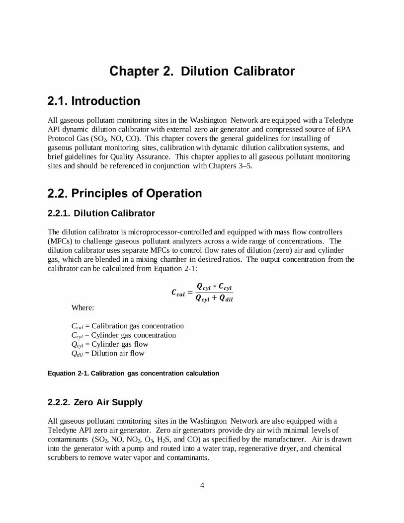
2.2.1. Dilution Calibrator The dilution calibrator is microprocessor-controlled and equipped with mass flow controllers (MFCs) to challenge gaseous pollutant analyzers across a wide range of concentrations. The dilution calibrator uses separate MFCs to control flow rates of dilution (zero) air and cylinder gas, which are blended in a mixing chamber in desired ratios. The output concentration from the calibrator can be calculated from Equation 2-1:

𝑪𝑪𝒄𝒄𝒄𝒄𝒄𝒄 =𝑸𝑸𝒄𝒄𝒄𝒄𝒄𝒄 ∗ 𝑪𝑪𝒄𝒄𝒄𝒄𝒄𝒄𝑸𝑸𝒄𝒄𝒄𝒄𝒄𝒄 + 𝑸𝑸𝒅𝒅𝒊𝒊𝒄𝒄

Where: Ccal = Calibration gas concentration Ccyl = Cylinder gas concentration Qcyl = Cylinder gas flow Qdil = Dilution air flow

Equation 2-1. Calibration gas concentration calculation

2.2.2. Zero Air Supply All gaseous pollutant monitoring sites in the Washington Network are also equipped with a Teledyne API zero air generator. Zero air generators provide dry air with minimal levels of contaminants (SO2, NO, NO2, O3, H2S, and CO) as specified by the manufacturer. Air is drawn into the generator with a pump and routed into a water trap, regenerative dryer, and chemical scrubbers to remove water vapor and contaminants.

5

For specific principles of operation for gaseous analyzers, see Chapters 3–5.

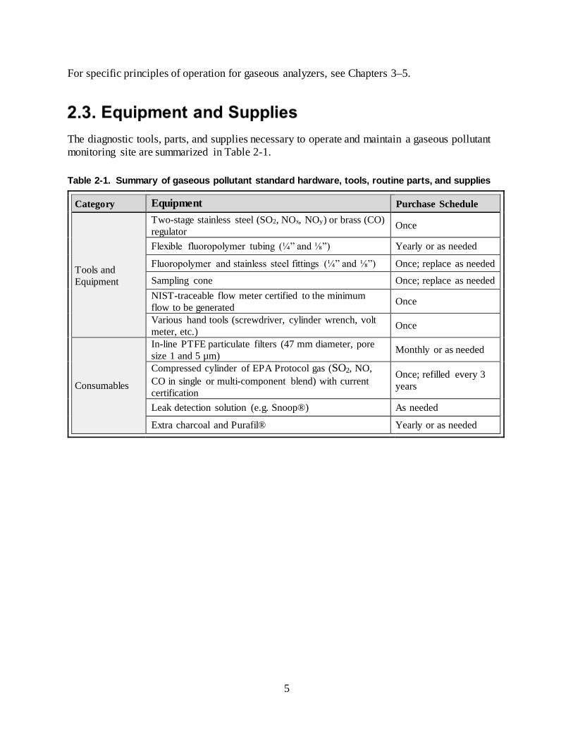
The diagnostic tools, parts, and supplies necessary to operate and maintain a gaseous pollutant monitoring site are summarized in Table 2-1. Table 2-1. Summary of gaseous pollutant standard hardware, tools, routine parts, and supplies

Category Equipment Purchase Schedule

Tools and Equipment

Two-stage stainless steel (SO2, NOx, NOy) or brass (CO) regulator Once

Flexible fluoropolymer tubing (¼” and ⅛”) Yearly or as needed

Fluoropolymer and stainless steel fittings (¼” and ⅛”) Once; replace as needed

Sampling cone Once; replace as needed NIST-traceable flow meter certified to the minimum flow to be generated Once

Various hand tools (screwdriver, cylinder wrench, volt meter, etc.) Once

Consumables

In-line PTFE particulate filters (47 mm diameter, pore size 1 and 5 µm) Monthly or as needed

Compressed cylinder of EPA Protocol gas (SO2, NO, CO in single or multi-component blend) with current certification

Once; refilled every 3 years

Leak detection solution (e.g. Snoop®) As needed

Extra charcoal and Purafil® Yearly or as needed

6

2.4.1. Siting 2.4.1.1. Siting criteria Siting requirements for gaseous pollutant analyzers vary by gas species and monitoring objective. Operators should refer to Chapters 3–5 and 40 CFR Part 58 Appendix E for requirements specific to the monitoring objective, including horizontal and vertical placement and spacing from minor sources, obstructions, trees and roadways. In general, probes must be located at least 1 horizontal and 1 vertical meter away from any supporting structure such as a wall. If a probe is located near a building or wall, it must have unrestricted airflow in a 180° arc facing upwind in the dominant wind direction during the season of highest expected concentrations. If there are any obstructions nearby, the distance between the obstruction and the probe must be at least twice the height of the obstruction minus the height of the probe. Probes should be located at least 10 meters outside the drip line of trees. 2.4.1.2. Shelter conditions Gaseous pollutant analyzers must be installed in clean, dry, temperature-controlled shelters with ample and reliable 110-120 VAC power. Shelters must be installed in a secure location safely accessible by monitoring staff. Shelters must be equipped with adequate HVAC systems to maintain room temperatures between 20 and 30° C year-round. Shelter temperature should not vary by more than ± 2°C per hour. Analyzers must not be positioned directly under the output vent of the air conditioner.

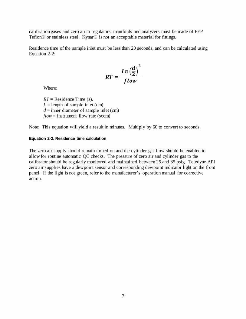
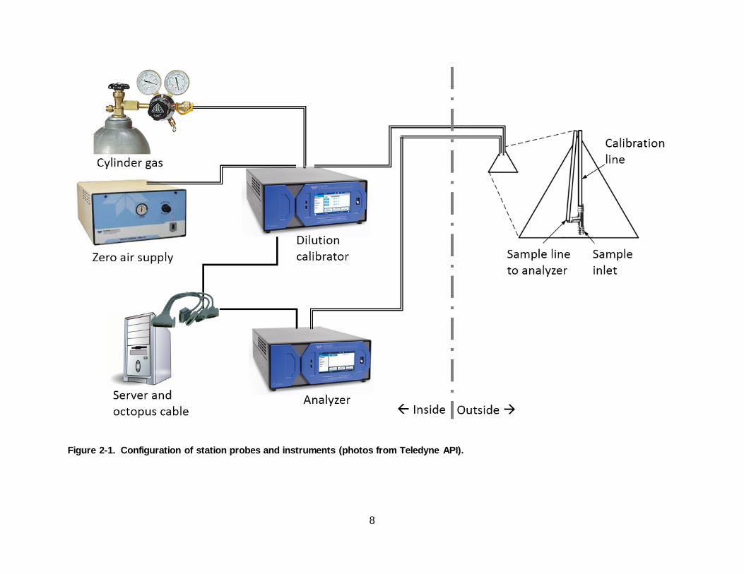
2.4.2. Installation 2.4.2.1. Probe configuration Gaseous pollutant monitoring sites contain a system of linked equipment to collect, analyze, calibrate, record and store ambient pollutant and calibration concentration data. To the extent possible, this system must be configured as shown in Figure 2-1. Both the analyzer and calibrator are connected to the server serially with a 9-pin cable. Cylinder gas and zero air are fed into the calibrator, which outputs calibration gas to a tee fitting at the probe tip outside the station. One end of the tee is open to ambient air and the other is attached to the analyzer inlet. This dual-probe configuration allows the calibration gas to be fed through the full sample path at near-ambient conditions in order to assess the complete sampling train, which is known as “through the probe” verification. The tee is sheltered under a funnel to protect the probe from precipitation. All Washington Network monitoring sites must use fluoropolymer tubing throughout the sampling train and calibration system. Recommended probe material is ¼” inch outer diameter PFA. Gas cylinder-to-calibrator lines are typically ⅛” outer diameter. All fittings that connect

7

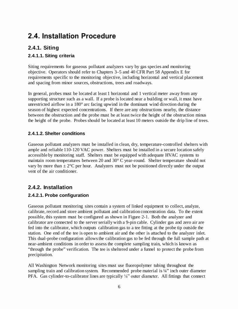
calibration gases and zero air to regulators, manifolds and analyzers must be made of FEP Teflon® or stainless steel. Kynar® is not an acceptable material for fittings. Residence time of the sample inlet must be less than 20 seconds, and can be calculated using Equation 2-2:

𝑹𝑹𝑹𝑹 = 𝑳𝑳𝛑𝛑 �𝒅𝒅𝟐𝟐�

𝟐𝟐

𝒇𝒇𝒄𝒄𝒇𝒇𝒇𝒇

Where: RT = Residence Time (s). L = length of sample inlet (cm) d = inner diameter of sample inlet (cm) flow = instrument flow rate (sccm)

Note: This equation will yield a result in minutes. Multiply by 60 to convert to seconds. Equation 2-2. Residence time calculation The zero air supply should remain turned on and the cylinder gas flow should be enabled to allow for routine automatic QC checks. The pressure of zero air and cylinder gas to the calibrator should be regularly monitored and maintained between 25 and 35 psig. Teledyne API zero air supplies have a dewpoint sensor and corresponding dewpoint indicator light on the front panel. If the light is not green, refer to the manufacturer’s operation manual for corrective action.

8

Figure 2-1. Configuration of station probes and instruments (photos from Teledyne API).

9

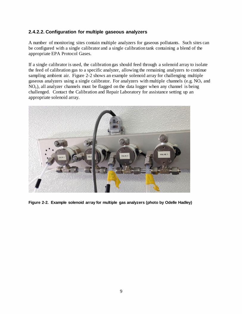
2.4.2.2. Configuration for multiple gaseous analyzers A number of monitoring sites contain multiple analyzers for gaseous pollutants. Such sites can be configured with a single calibrator and a single calibration tank containing a blend of the appropriate EPA Protocol Gases. If a single calibrator is used, the calibration gas should feed through a solenoid array to isolate the feed of calibration gas to a specific analyzer, allowing the remaining analyzers to continue sampling ambient air. Figure 2-2 shows an example solenoid array for challenging multiple gaseous analyzers using a single calibrator. For analyzers with multiple channels (e.g. NOx and NOy), all analyzer channels must be flagged on the data logger when any channel is being challenged. Contact the Calibration and Repair Laboratory for assistance setting up an appropriate solenoid array.

Figure 2-2. Example solenoid array for multiple gas analyzers (photo by Odelle Hadley)

10

The quality control (QC) procedure consists of both automatic quality control checks and site visits at routine intervals. All QC checks must be triggered through Envidas Ultimate in order to ensure consistency in quality control check procedures throughout the Washington Network and to ensure that the results are captured by the data acquisition system. Note: A number of terms for various quality control checks and challenge points exist throughout EPA literature, existing SOPs, the Envidas Ultimate framework, etc. This SOP adopts the uniform terminology of “Primary QC Check” and “Secondary QC Check” in place of these terms. These terms are paired with their corresponding EPA terms in Table 2-2 below. Table 2-2. Ecology and EPA quality control check terms

Ecology Term EPA Term Number of

Target Points Ecology Target Point

Term EPA Target Point Term

Primary QC Check

One-Point QC Check

2-3 including zero

Primary QC Point 1; (optional) Primary QC Point 2

QC Check Concentration; Precision Point

Secondary QC Check

Zero/Span Check; Multi-Point Verification

3-4 including zero

Secondary QC Point 1; (optional) Secondary QC Point 2

Span Check Value

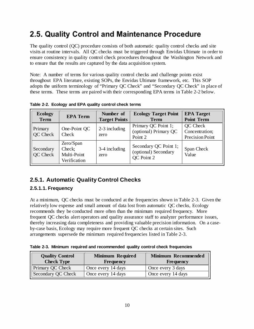
2.5.1. Automatic Quality Control Checks 2.5.1.1. Frequency At a minimum, QC checks must be conducted at the frequencies shown in Table 2-3. Given the relatively low expense and small amount of data lost from automatic QC checks, Ecology recommends they be conducted more often than the minimum required frequency. More frequent QC checks alert operators and quality assurance staff to analyzer performance issues, thereby increasing data completeness and providing valuable precision information. On a case-by-case basis, Ecology may require more frequent QC checks at certain sites. Such arrangements supersede the minimum required frequencies listed in Table 2-3. Table 2-3. Minimum required and recommended quality control check frequencies

Quality Control Check Type

Minimum Required Frequency

Minimum Recommended Frequency

Primary QC Check Once every 14 days Once every 3 days Secondary QC Check Once every 14 days Once every 14 days

11

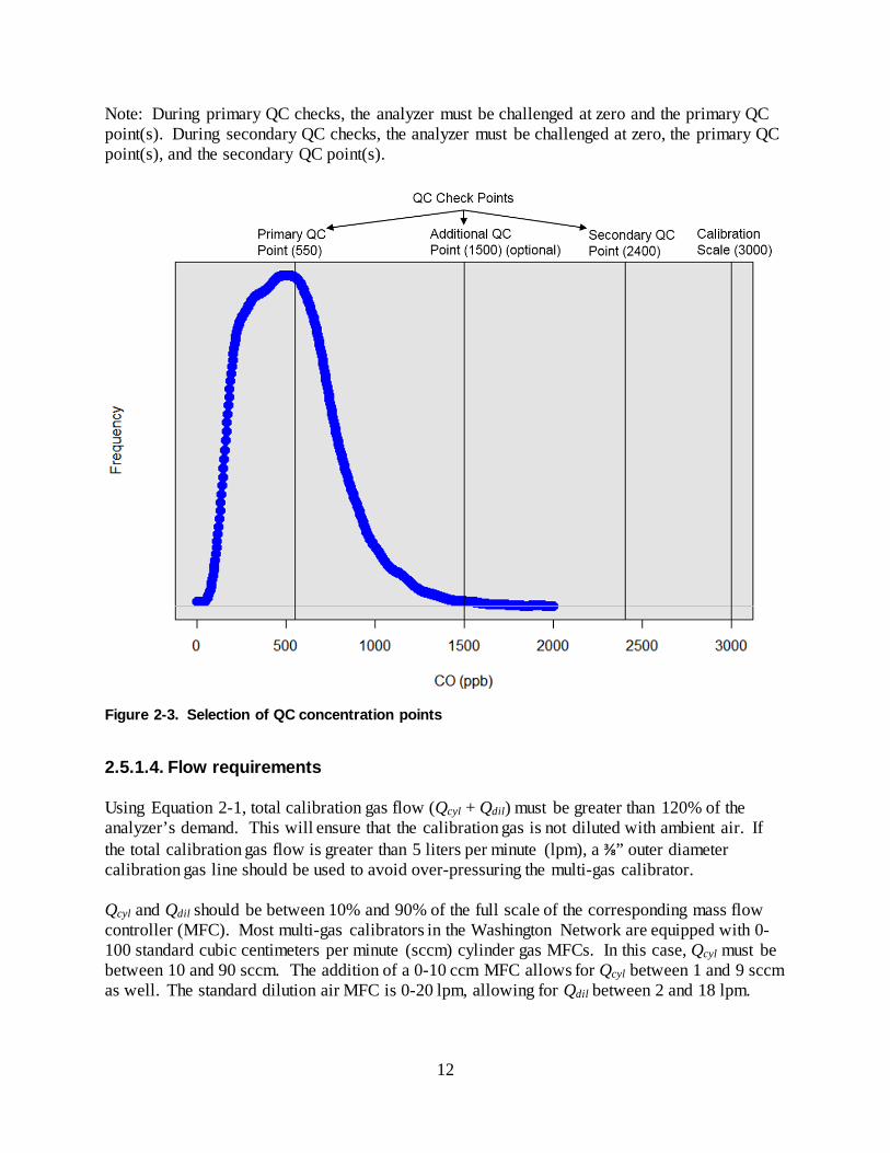
2.5.1.2. Timing Automatic QC checks should be timed during the hours of lowest expected concentrations, which are typically between 12 a.m. and 4 a.m. Start times should be selected to minimize the number of data hours lost, given that hours with more than 15 minutes of data missing are not valid. QC checks lasting up to 88 minutes should be timed to start at 0:46 after the hour so that only the middle hour is lost. For example, if a QC check starts at 1:46 and lasts until 3:14, only the 2:00 hour will be lost. Both the 1:00 and 3:00 hours have enough 1-minute sample data to be considered valid. It is recommended that secondary QC checks be scheduled for every other Monday morning so that operators are able to promptly respond to issues raised by the QC check early in the work week. 2.5.1.3. QC check concentrations QC check concentrations should be chosen based on the monitoring objectives and the concentrations routinely measured at the monitoring site. The recommended approach is described below and illustrated in Figure 2-3.

1. Plot the most recent 3 years of 1-hour concentration data, excluding any obvious outliers. Figure 2-3 shows an example of CO data from a near-road monitoring site.

2. Select a concentration at or near the maximum. This value is 2000 ppb in the example shown in Figure 2-3.

3. Multiply the maximum concentration by 1.5 to establish the calibration scale (3000 ppb in this example). The instrument should be calibrated to this concentration (see Section 2.5.3.)

4. Multiply the calibration scale by 0.8 to find the secondary QC point, which is measured during a secondary QC check (2400 ppb in this example).

5. Select a point at or near the peak of the data distribution for the primary QC point (550 ppb in this example). If this point is below the MDL of the instrument or the capabilities of the calibration system, the operator should select the lowest point that can be practically generated and measured. All primary QC points must fall within EPA’s prescribed ranges of 0.005 and 0.08 ppm for SO2 and NO2 and 0.5 and 5 ppm for CO.

6. At sites whose primary purpose is NAAQS comparison and whose concentrations frequently approach or exceed the NAAQS, the level of the NAAQS should be chosen as the primary QC point. Alternatively, the analyzer can be challenged at the level of the NAAQS as an additional primary QC point (primary QC point 2), with primary QC point 1 determined by the method in step 5. If the NAAQS is chosen as a primary QC point, the calibration scale should be at least 1.5 times the NAAQS.

7. Operators can select a concentration approximately halfway between the primary and secondary QC points for an optional additional QC point during primary or secondary QC checks (1500 ppb in this example).

12

Note: During primary QC checks, the analyzer must be challenged at zero and the primary QC point(s). During secondary QC checks, the analyzer must be challenged at zero, the primary QC point(s), and the secondary QC point(s).

Figure 2-3. Selection of QC concentration points 2.5.1.4. Flow requirements Using Equation 2-1, total calibration gas flow (Qcyl + Qdil) must be greater than 120% of the analyzer’s demand. This will ensure that the calibration gas is not diluted with ambient air. If the total calibration gas flow is greater than 5 liters per minute (lpm), a ⅜” outer diameter calibration gas line should be used to avoid over-pressuring the multi-gas calibrator. Qcyl and Qdil should be between 10% and 90% of the full scale of the corresponding mass flow controller (MFC). Most multi-gas calibrators in the Washington Network are equipped with 0-100 standard cubic centimeters per minute (sccm) cylinder gas MFCs. In this case, Qcyl must be between 10 and 90 sccm. The addition of a 0-10 ccm MFC allows for Qcyl between 1 and 9 sccm as well. The standard dilution air MFC is 0-20 lpm, allowing for Qdil between 2 and 18 lpm.

13

2.5.1.5. Acceptance criteria Acceptance criteria vary by parameter and are summarized in Table 2-4. Table 2-4. QC check acceptance criteria

Parameter Zero Limits Primary/Secondary QC Check Point Limits

SO2 ± 1.0 ppb ± 10% NO and NO2 ± 1.5 ppb ± 15% CO ± 50 ppb ± 10%

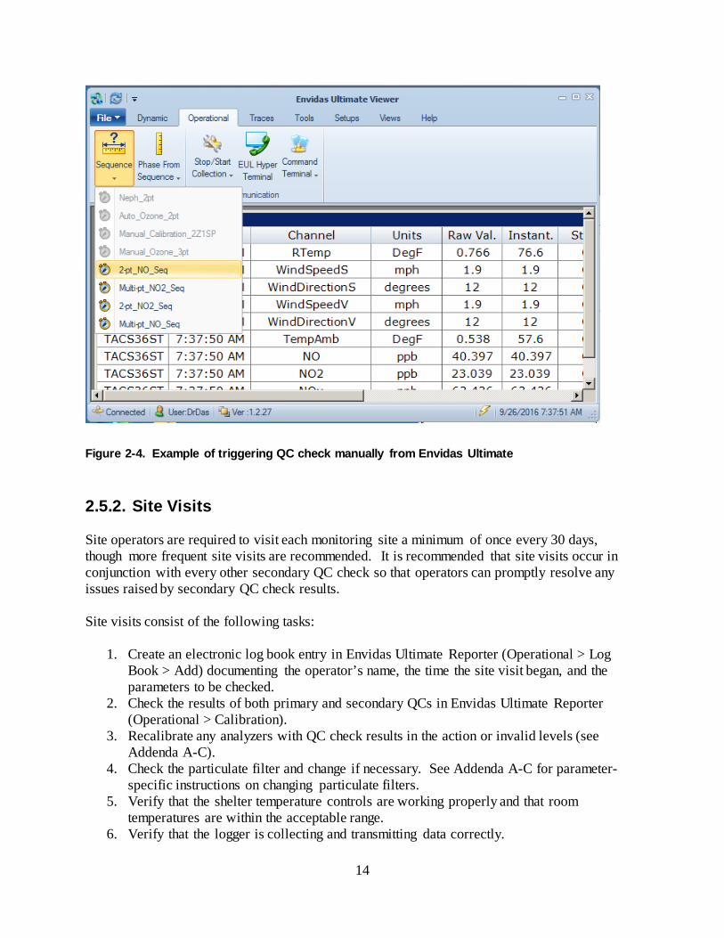
For further information on parameter-specific action levels, see Chapters 3–5. 2.5.1.6. Manually triggering QC checks Occasionally, operators may need to manually trigger primary or secondary QC checks. This is necessary if automatic QC checks fail to run properly or if operators need to initiate additional QC checks before and after recalibration. Even when manually triggering QC checks, operators must initiate the QC check from Envidas Ultimate and not from the calibrator itself. This ensures that all results are captured by the data acquisition system and are reportable to EPA’s Air Quality System (AQS). To trigger a QC check manually, navigate to the Operational tab in Envidas Ultimate Viewer and select Calibration > Sequence, then select the name of the primary or secondary QC sequence to trigger as shown in Figure 2-4.

14

Figure 2-4. Example of triggering QC check manually from Envidas Ultimate

2.5.2. Site Visits Site operators are required to visit each monitoring site a minimum of once every 30 days, though more frequent site visits are recommended. It is recommended that site visits occur in conjunction with every other secondary QC check so that operators can promptly resolve any issues raised by secondary QC check results. Site visits consist of the following tasks:

1. Create an electronic log book entry in Envidas Ultimate Reporter (Operational > Log Book > Add) documenting the operator’s name, the time the site visit began, and the parameters to be checked.

2. Check the results of both primary and secondary QCs in Envidas Ultimate Reporter (Operational > Calibration).

3. Recalibrate any analyzers with QC check results in the action or invalid levels (see Addenda A-C).

4. Check the particulate filter and change if necessary. See Addenda A-C for parameter-specific instructions on changing particulate filters.

5. Verify that the shelter temperature controls are working properly and that room temperatures are within the acceptable range.

6. Verify that the logger is collecting and transmitting data correctly.

15

7. Check each instrument’s diagnostics in Envidas Ultimate Reporter for indications of any instrument problems (Operational > Digital > Diagnostic).

8. Create an electronic log book entry documenting any changes made to the site, any periods of invalid data, and any unusual air quality conditions that may affect sample concentrations (e.g., wildfires, nearby construction impacts from diesel equipment, etc.).

9. Operators may record QC results and additional site visit information on the “Gaseous Pollutant QC Form.” These records may be useful for tracking instrument diagnostics, identifying drift and troubleshooting malfunctions. In certain cases, Ecology may require operators to submit this form following monthly site visits. Contact the Quality Assurance unit for a copy of this form.

2.5.3. Analyzer Calibration A gaseous pollutant analyzer’s calibration must be checked:

• upon installation; • following any repair or part replacement; • after sample lines are cleaned or replaced; • when failing QC checks indicate that the analyzer is out of calibration.

If recalibrating an analyzer, operators must perform an “as found” primary QC check before recalibration and an “as left” primary QC check after recalibration. For specific instructions on recalibrating gaseous pollutant analyzers, refer to the instrument-specific operation manuals and Chapters 3–5.

2.5.4. Calibration System Maintenance Table 2-5 summarizes the required maintenance schedule for the calibration system. This table does not include maintenance for the O3 module components necessary for NOx and NOy monitoring. For calibrators with an O3 generator installed, the operator should refer to Chapter 4 and the manufacturer’s operation manual for the specific maintenance schedule and procedures. Operators must document annual maintenance completed on the “Multigas Calibrator Annual Maintenance Form” and return the completed form to Ecology within 30 days of the completion date. Contact the Quality Assurance unit for a copy of this form. Maintenance procedures for the gaseous pollutant analyzers are described in Chapters 3–5.

16

Table 2-5. Summary of required dynamic dilution calibrator maintenance

Component Procedure Frequency Section

Dilution calibrator

Diagnostic data verification Monthly or after any maintenance 2.5.4.1

Flow check and calibration Annually or after any maintenance 2.5.4.2

Leak check Annually or after any maintenance 2.5.4.3

Pneumatic line inspection Annually 2.5.4.4 Zero air source Zero air generator maintenance Annually 2.5.4.5

Cylinder gas Verify cylinder gas certification Annually 2.5.4.6

Station Clean or replace sample and calibration lines Annually 2.5.4.7

2.5.4.1. Verify calibrator diagnostic data Diagnostic data, referred to by Teledyne API as “test functions,” can be used to predict and diagnose instrument failures. Diagnostic data is collected every 30 minutes by Envidas Ultimate and retained for 9 months. The acceptable ranges for these diagnostic parameters are listed in the “Acceptable Limits in Use” column of the Final Calibrated Test and Validation Data Sheet shipped with the instrument. Values outside these acceptable ranges indicate a failure in one or more of the calibrator’s subsystems. Parameters whose values are within acceptable ranges but have significantly deviated from those recorded on the factory data sheet may also indicate a failure. Table 2-6 below does not include test functions associated with the O3 module components. Table 2-6. Summary of dilution calibrator diagnostic data

Diagnostic Parameter Interpretation

CAL PRES Measures the pressure delivered to gas MFCs. Possible causes of faults such as the MFC PRESSURE WARNING.

DIL PRES Measures the pressure delivered to diluent MFC. Possible causes of faults such as the MFC PRESSURE WARNING.

17

2.5.4.2. Calibrator flow check and calibration The output flow of the calibrator should be verified annually and after calibration of the internal digital-to-analog converter (DAC). The flow check procedure verifies the output flow of each MFC at 20 incremental points corresponding to drive voltages from 0 to 5000 mVDC. Directions for the flow check and calibration can be found in the manufacturer’s operation manual. 2.5.4.3. Calibrator leak check

An automatic leak check must be performed annually and after any maintenance or repair. Directions can be found in the manufacturer’s operation manual.

2.5.4.4. Calibrator pneumatic line inspection Visually inspect the lines inside the calibrator for any signs of dirt, condensation, obstructions, cracking, kinks, obstruction, or any other damage. Clean or replace the lines as needed. 2.5.4.5. Zero air generator maintenance The charcoal and Purafil® in the zero air source canisters and the particulate filter on the zero air generator must be replaced annually. A leak check must be conducted following any maintenance. Directions can be found in the manufacturer’s operation manual. If evidence of zero air contamination is present, the HC scrubber, CO scrubber, and regenerative dryer should also be replaced. Refer to the manufacturer’s operation manual or contact the Calibration and Repair Laboratory for assistance. 2.5.4.6. Verify cylinder gas certification All calibration gases used within the Washington Network must have current certification. Expiration dates of EPA Protocol gas cylinders should be checked annually to ensure that cylinders will be valid for the duration of the next annual maintenance cycle.

BOX TEMP

Typically ~ 7°C warmer than ambient temperature. If out of range, ensure that:

the exhaust fan is running, and there is sufficient ventilation area to all sides of the

instrument.

CLOCKTIME If calibrator clock is not correct, battery in clock chip on CPU board may be dead.

18

2.5.4.7. Clean or replace sample and calibration lines

Sample and calibration lines must be cleaned or replaced when necessary, but at least annually. Dust, bugs, moisture, organic compounds, elemental carbon, and other contaminants can build up in the lines over time and affect gas flows and concentrations. It is recommended that operators replace sample lines with new tubing annually. Operators can elect to clean sample lines with rubbing alcohol followed by deionized water and pressurized zero air. If cleaning the lines, operators must first disconnect them from the instruments and ensure that no moisture remains in the sample line before reconnecting them.

All gaseous pollutant monitoring sites in the Washington Network are equipped with loggers running the Envidas Ultimate data acquisition system. These servers must be configured to collect and telemeter 1-minute and 1-hour average concentrations. SO2 monitoring sites must also collect and telemeter 5-minute average concentrations in order to meet the requirement to report maximum hourly 5-minute average concentrations to EPA. The channel configurations and diagnostic settings for the calibrator channel are shown below. For analyzer-specific channel and diagnostic configurations, see Chapters 3–5.

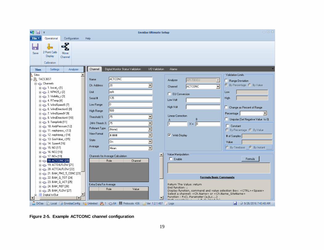
2.6.1. Envidas Channel Configuration All loggers at gaseous pollutant sites in the Washington Network must be configured with a channel to capture the actual concentration of calibration gas delivered by the calibrator. This channel is typically called ACTCONC for “actual concentration.” Figure 2-5 shows the correct configuration for the ACTCONC channel in Envidas Ultimate.

19

Figure 2-5. Example ACTCONC channel configuration

20

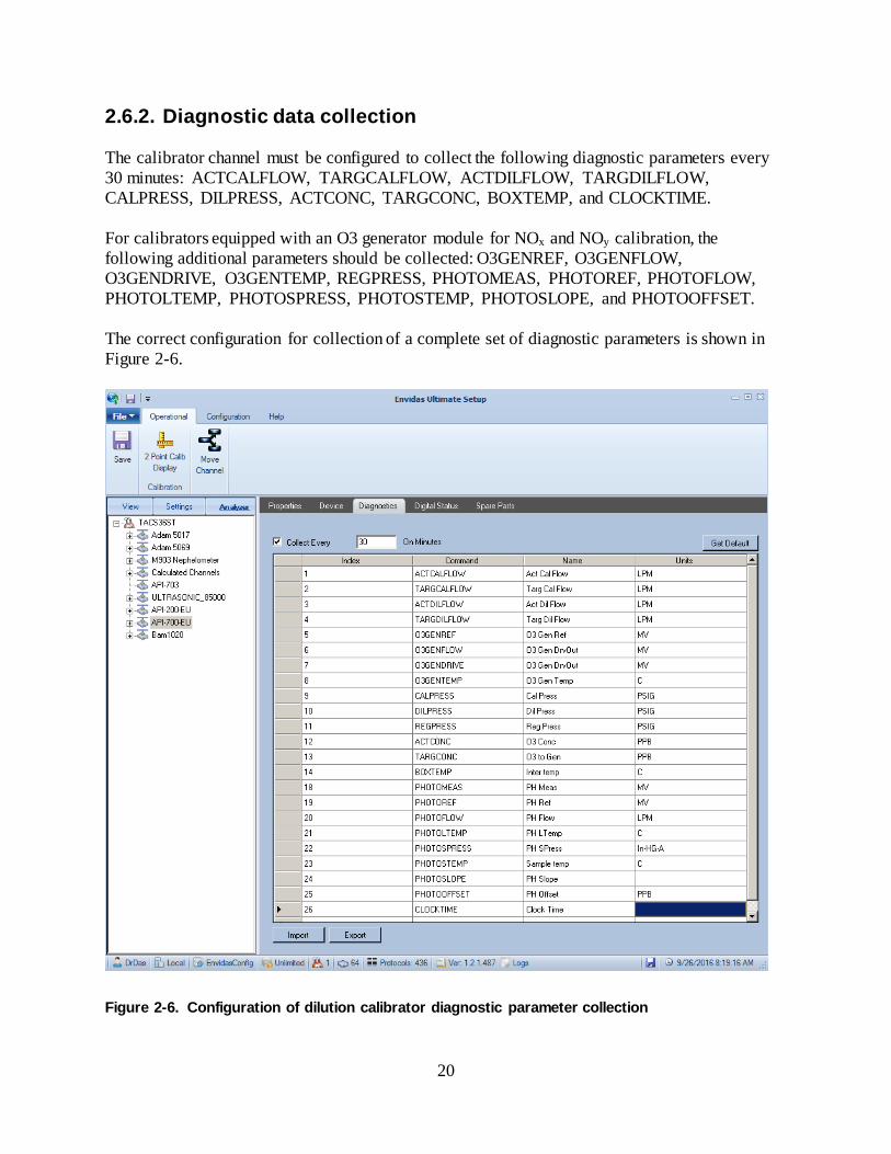
2.6.2. Diagnostic data collection The calibrator channel must be configured to collect the following diagnostic parameters every 30 minutes: ACTCALFLOW, TARGCALFLOW, ACTDILFLOW, TARGDILFLOW, CALPRESS, DILPRESS, ACTCONC, TARGCONC, BOXTEMP, and CLOCKTIME. For calibrators equipped with an O3 generator module for NOx and NOy calibration, the following additional parameters should be collected: O3GENREF, O3GENFLOW, O3GENDRIVE, O3GENTEMP, REGPRESS, PHOTOMEAS, PHOTOREF, PHOTOFLOW, PHOTOLTEMP, PHOTOSPRESS, PHOTOSTEMP, PHOTOSLOPE, and PHOTOOFFSET. The correct configuration for collection of a complete set of diagnostic parameters is shown in Figure 2-6.

Figure 2-6. Configuration of dilution calibrator diagnostic parameter collection

21

The operator is responsible for preliminary level review and data validation of collected sample data. At a minimum, operators must review all quality control check results in a timely fashion in order to catch problems early and prevent data loss. It is recommended that operators review calibration results via the data acquisition system software each Monday morning. Operators should also review data for reasonability and comparability with other like monitors. Operators must notify the Quality Assurance unit via email when invalid data are identified. When required by Ecology, operators must submit the completed “Gaseous Pollutant QC Form” to the Quality Assurance unit by the 10th of the following month. The Quality Assurance unit is responsible for final level data validation. Data validity is evaluated using a number of criteria, including but not limited to the results and frequency of quality control checks, performance audit results, and diagnostic data. The critical, operational and systematic criteria used by the QA unit to help determine data validity are summarized in the most current version of EPA’s criteria pollutant validation templates. In general, when an analyzer fails a primary or secondary QC, data is considered invalid between the most recent preceding passing QC check and the earliest passing QC check following the failure. For more detailed information on data review and validation, please refer to Ecology’s Air Monitoring Documentation, Data Review, and Validation Procedure.

https://www3.epa.gov/ttn/amtic/files/ambient/pm25/qa/appd_validation_template_amtic.pdf

22

Sulfur Dioxide (SO2) Monitoring

This chapter describes Ecology’s procedures for monitoring trace- and ambient-level SO2 concentrations using the Teledyne API T100U and T100 analyzers. It includes procedures for installation, operation, quality control, maintenance, and data acquisition. It is intended to be used with the manufacturer’s model-specific operation manual and Chapter 2, which describes general procedures for gaseous pollutant monitoring and calibration with dynamic dilution calibration systems.

The SO2 analysis method is based on the principle of characteristic fluorescence released by excited SO2 when subject to ultraviolet (UV) light. The SO2 analyzer collects ambient samples and detects the decaying radiation emitted by SO2 present in the sample with the photo multiplier tube (PMT). It then converts the signal to a measurable voltage that corresponds to ambient concentrations. A wavelength range of approximately 190–230 nm is used to charge SO2 to its excited state and a longer wavelength near 330 nm with lower energy is used in the PMT to measure fluorescence. Both the Teledyne API T100 and T100U are equipped with a scrubber to remove hydrocarbons that fluoresce similarly to SO2 and could create positive interference. The primary difference between T100 and the modified T100U is how the PMT and UV reference signals are acquired and processed. The T100 achieves stability through use of an optical shutter that compensates for sensor drift and a reference detector that corrects for UV lamp intensity variations. The T100U, on the other hand, employs a sync demodulator to capture the dark and light PMT and UV reference signals several times per second and synchronize the operation of the UV source with these measurements. This method of signal processing minimizes the error that could occur when changing offsets, especially for an instrument designated to operate near its detection limit. Thus, the T100U is more ideal for monitoring SO2 at near zero concentrations and is required for trace-level SO2 monitoring in the Washington Network.

In addition to the standard equipment in Table 2-1, operators will need to purchase a pump rebuild kit annually.

In addition to the siting criteria described in Section 2.4, the SO2 sample probe must be located 2–15 m above ground level.

23

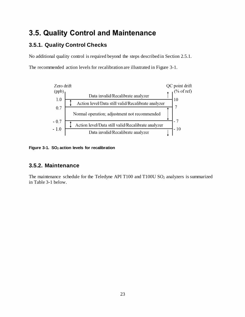
3.5.1. Quality Control Checks No additional quality control is required beyond the steps described in Section 2.5.1. The recommended action levels for recalibration are illustrated in Figure 3-1.

Figure 3-1. SO2 action levels for recalibration

3.5.2. Maintenance The maintenance schedule for the Teledyne API T100 and T100U SO2 analyzers is summarized in Table 3-1 below.

24

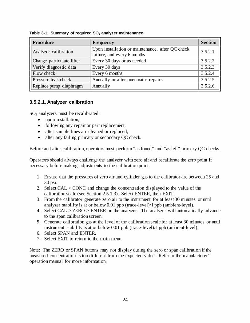
Table 3-1. Summary of required SO2 analyzer maintenance

Procedure Frequency Section

Analyzer calibration Upon installation or maintenance, after QC check failure, and every 6 months 3.5.2.1

Change particulate filter Every 30 days or as needed 3.5.2.2 Verify diagnostic data Every 30 days 3.5.2.3 Flow check Every 6 months 3.5.2.4 Pressure leak check Annually or after pneumatic repairs 3.5.2.5 Replace pump diaphragm Annually 3.5.2.6

3.5.2.1. Analyzer calibration SO2 analyzers must be recalibrated:

• upon installation; • following any repair or part replacement; • after sample lines are cleaned or replaced; • after any failing primary or secondary QC check.

Before and after calibration, operators must perform “as found” and “as left” primary QC checks. Operators should always challenge the analyzer with zero air and recalibrate the zero point if necessary before making adjustments to the calibration point.

1. Ensure that the pressures of zero air and cylinder gas to the calibrator are between 25 and 30 psi.

2. Select CAL > CONC and change the concentration displayed to the value of the calibration scale (see Section 2.5.1.3). Select ENTER, then EXIT.

3. From the calibrator, generate zero air to the instrument for at least 30 minutes or until analyzer stability is at or below 0.01 ppb (trace-level)/1 ppb (ambient-level).

4. Select CAL > ZERO > ENTER on the analyzer. The analyzer will automatically advance to the span calibration screen.

5. Generate calibration gas at the level of the calibration scale for at least 30 minutes or until instrument stability is at or below 0.01 ppb (trace-level)/1 ppb (ambient-level).

6. Select SPAN and ENTER. 7. Select EXIT to return to the main menu.

Note: The ZERO or SPAN buttons may not display during the zero or span calibration if the measured concentration is too different from the expected value. Refer to the manufacturer’s operation manual for more information.

25

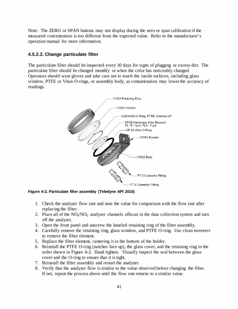
3.5.2.2. Change particulate filter The particulate filter should be inspected every 30 days for signs of plugging or excess dirt. The particulate filter should be changed monthly or when the color has noticeably changed. Operators should wear gloves and take care not to touch the glass window with bare hands, as contamination may lower the accuracy of readings.

Figure 3-2. Particulate filter assembly (Teledyne API 2016)

1. Check the analyzer flow rate and note the value for comparison with the flow rate after replacing the filter.

2. Turn off the analyzer. 3. Open the front panel and unscrew the knurled retaining ring of the filter assembly. 4. Carefully remove the retaining ring, glass window, and PTFE O-ring. Use tweezers to

remove the filter element. 5. Replace the filter element, centering it in the bottom of the holder. 6. Reinstall the PTFE O-ring (notches face up), the glass cover, and the retaining ring in the

order shown in Figure 3-2. Hand tighten. Visually inspect the seal between the glass cover and the O-ring to ensure that it is tight. If the retaining ring is not tightened enough, it can result in a leak in the sample flow.

7. Reinstall the filter assembly and restart the analyzer. 8. Verify that the analyzer flow is similar to the value observed before changing the filter.

If not, repeat the process above until the flowrate returns to a similar value.

26

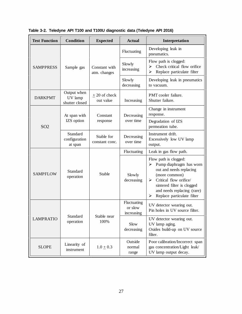
3.5.2.3. Verify diagnostic data At a minimum, operators must review the diagnostic data collected since the last site visit every 30 days to identify any problems with the analyzer’s operation. However, in order to identify potential problems and prevent data loss, it is recommended that operators review diagnostic data on Monday mornings following the secondary quality control check (i.e., every two weeks). Table 3-2 below shows the diagnostic parameters available and their interpretation.

27

Table 3-2. Teledyne API T100 and T100U diagnostic data (Teledyne API 2016)

Test Function Condition Expected Actual Interpretation

SAMPPRESS

Sample gas Constant with atm. changes

Fluctuating Developing leak in pneumatics.

Slowly increasing

Flow path is clogged: Check critical flow orifice Replace particulate filter

Slowly decreasing

Developing leak in pneumatics to vacuum.

DARKPMT Output when

UV lamp shutter closed

+ 20 of check out value

Increasing

PMT cooler failure. Shutter failure.

SO2

At span with IZS option

Constant response

Decreasing over time

Change in instrument response.

Degradation of IZS permeation tube.

Standard configuration

at span

Stable for constant conc.


Instrument drift. Excessively low UV lamp output.

SAMPFLOW Standard operation Stable

Fluctuating Leak in gas flow path.

Slowly decreasing

Flow path is clogged: Pump diaphragm has worn

out and needs replacing (more common)

Critical flow orifice/ sintered filter is clogged and needs replacing (rare)

Replace particulate filter

LAMPRATIO Standard operation

Stable near 100%

Fluctuating or slow

increasing

UV detector wearing out. Pin holes in UV source filter.

Slow decreasing

UV detector wearing out. UV lamp aging. Oxides build-up on UV source filter.

SLOPE Linearity of instrument 1.0 + 0.3

Outside normal range

Poor calibration/Incorrect span gas concentration/Light leak/ UV lamp output decay.

28

3.5.2.4. Flow check In addition to reviewing the analyzer’s reported flow via diagnostics, operators should verify the analyzer’s flow every 6 months using a certified, NIST-traceable flow meter.

1. Disconnect the sample inlet tubing from the rear panel SAMPLE port. 2. Attach the outlet port of a flow meter to the sample inlet port on the rear panel. Ensure

that the inlet to the flow meter is at atmospheric pressure. 3. The sample flow measured with the external flow meter should be within 10% of the

indicated flow. The sample flow should be between 550 and 600 sccm.

Low flows indicate that the pneumatic pathways are blocked. Refer to the manufacturer’s operation manual or contact the Calibration & Repair Laboratory for troubleshooting assistance. 3.5.2.5. Leak check To perform a leak check, operators must pressurize the instrument to 10 psi and hold the pressure for about 10 minutes. This can be achieved with a hand-held pressure pump with pressure gauge or with a tank of pressured gas (ultrapure air or nitrogen) with a two-stage regulator adjusted to < 15 psi, a shutoff valve and a pressure gauge.

1. Turn off the analyzer and remove the instrument cover. 2. Install the pressure source on the SAMPLE inlet on the rear panel of the instrument. 3. Pressurize the instrument to approximately 10 psi, allowing enough time for full

pressurization through the critical orifice. Do not exceed 15 psi. 4. Turn off pressure to the instrument and allow to sit for 10 minutes. If the pressure gauge

measures a loss exceeding 0.8 psi during that time, there is a leak in the pneumatics. 5. If the leak check fails, use a liquid leak detector (e.g. Snoop®) to search for leaks.

Pressurize the instrument to 10 psi and check each tube connection (fittings, hose clamps) with solution and look for bubbles. Wipe off all leak detection fluid before reconnecting sample lines to ensure that fluid is not sucked into the instrument.

6. Reconnect the sample and exhaust lines, and replace the instrument cover. 3.5.2.6. Replace pump diaphragm Low flow or no flow can be a sign of worn-out seals in the pump. Pumps should be rebuilt annually using the Teledyne API pump rebuild kit. Detailed instructions are included with the rebuild kit.

29

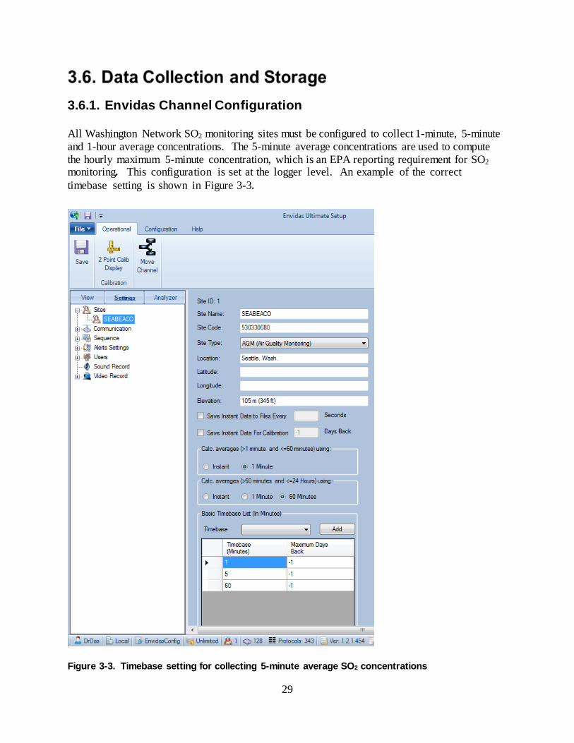
3.6.1. Envidas Channel Configuration All Washington Network SO2 monitoring sites must be configured to collect 1-minute, 5-minute and 1-hour average concentrations. The 5-minute average concentrations are used to compute the hourly maximum 5-minute concentration, which is an EPA reporting requirement for SO2 monitoring. This configuration is set at the logger level. An example of the correct timebase setting is shown in Figure 3-3.

Figure 3-3. Timebase setting for collecting 5-minute average SO2 concentrations

30

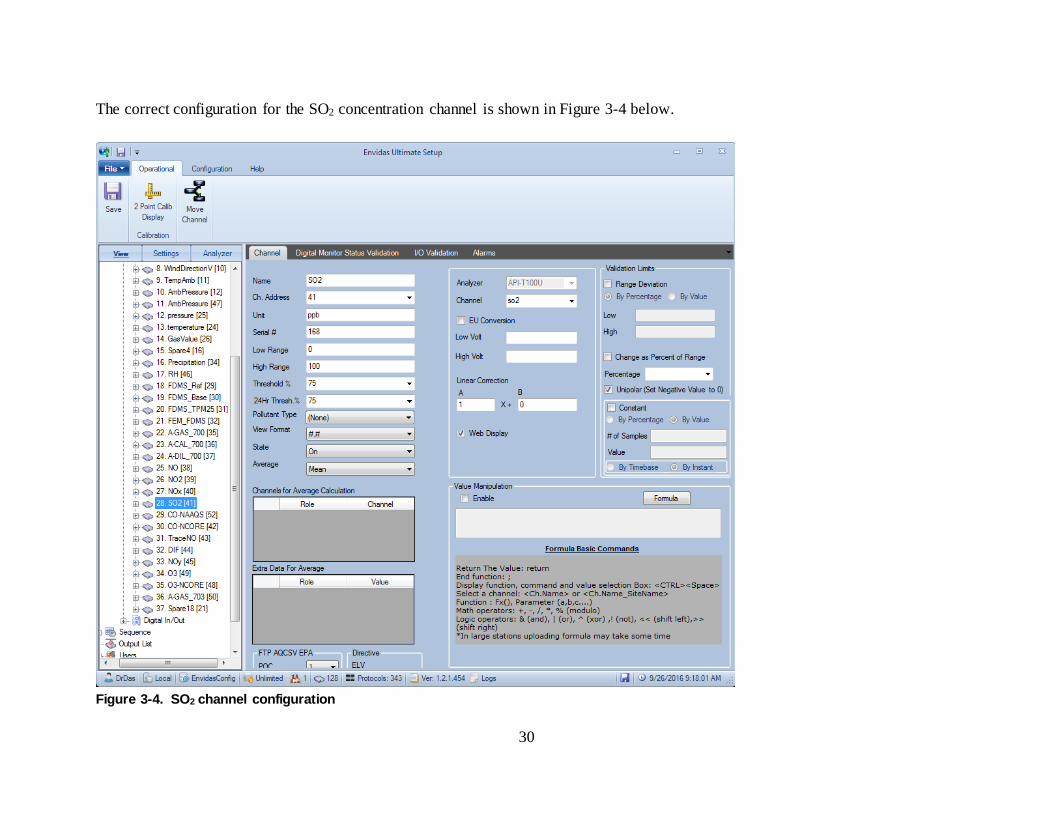
The correct configuration for the SO2 concentration channel is shown in Figure 3-4 below.

Figure 3-4. SO2 channel configuration

31

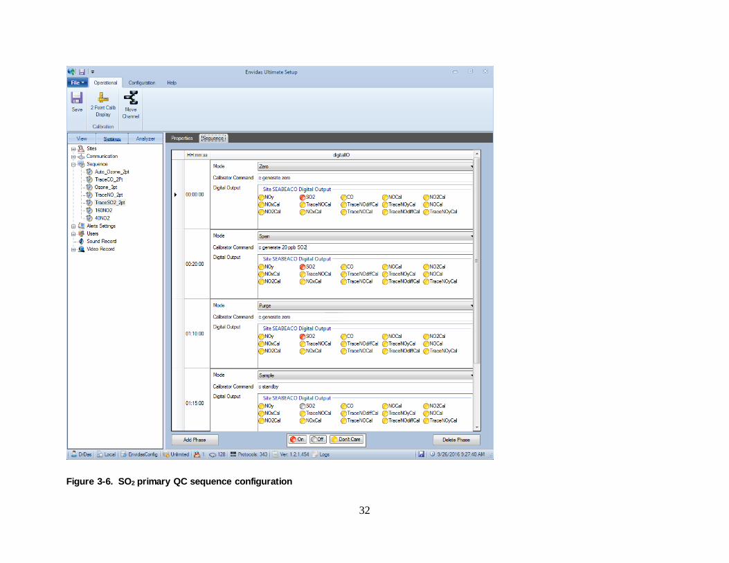
The configuration for a primary QC check set to run every 2 days is shown in Figure 3-5 through Figure 3-8. This sequence can be modified with an additional point for a secondary QC check. All phases should last a minimum of 30 minutes. For non-zero points, the reference value should be a 2-minute channel average of the ACTCONC channel (Figure 3-8).

Figure 3-5. SO2 primary QC sequence properties

32

Figure 3-6. SO2 primary QC sequence configuration

33

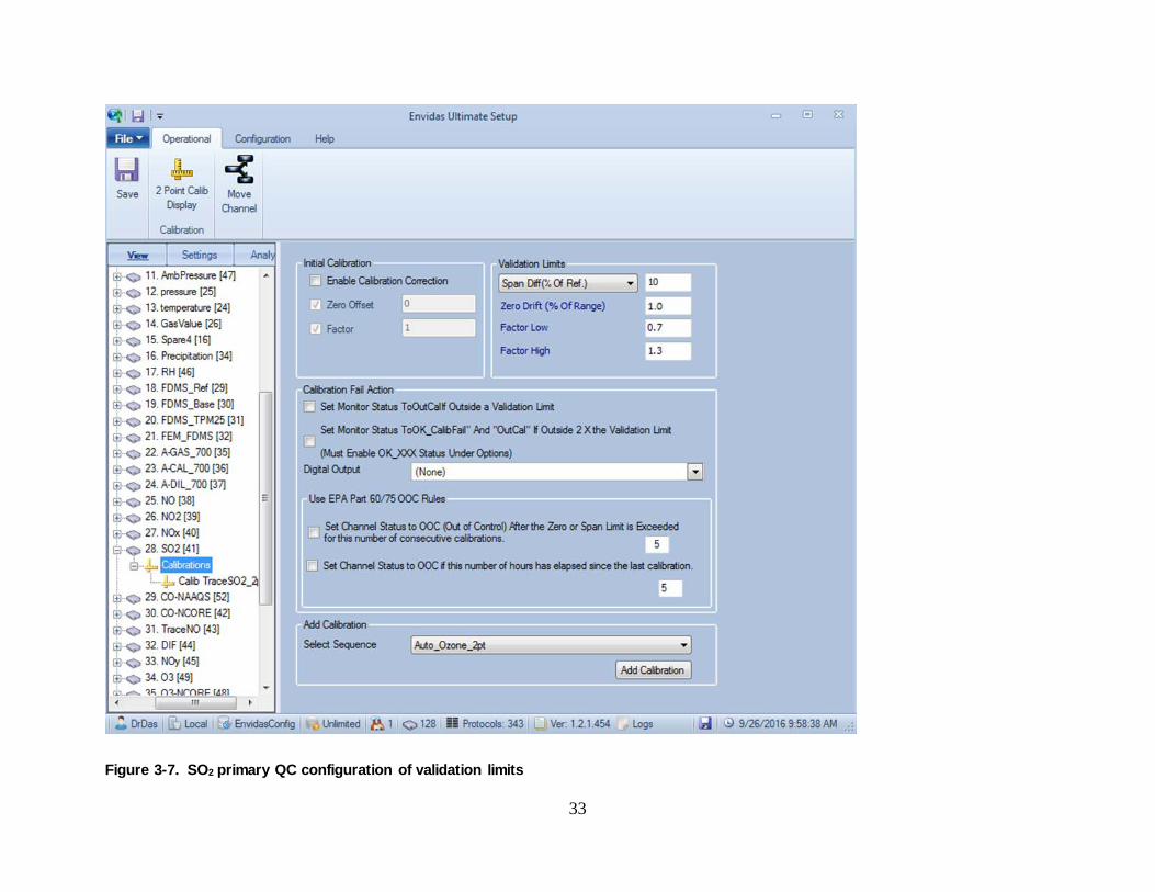
Figure 3-7. SO2 primary QC configuration of validation limits

34

Figure 3-8. SO2 primary QC configuration of phases and reference values

35

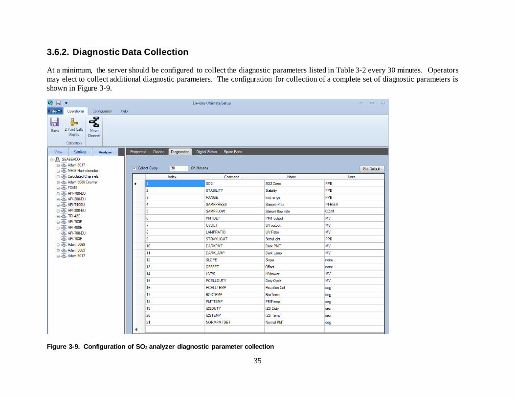
3.6.2. Diagnostic Data Collection At a minimum, the server should be configured to collect the diagnostic parameters listed in Table 3-2 every 30 minutes. Operators may elect to collect additional diagnostic parameters. The configuration for collection of a complete set of diagnostic parameters is shown in Figure 3-9.

Figure 3-9. Configuration of SO2 analyzer diagnostic parameter collection

36

Nitrogen Oxides (NOx) and Reactive Nitrogen (NOy) Monitoring

This chapter describes Ecology’s procedures for monitoring trace- and ambient-level nitrogen oxides (NOx) and reactive nitrogen compounds (NOy) using the Teledyne API M200EU and API T200U-NOy and other analyzers. The concentration of nitrogen oxides (NOx) in ambient air is defined as the sum of the concentration of nitric oxide (NO) and nitrogen dioxide (NO2). Total reactive nitrogen compounds (NOy) are precursors for ozone (O3) and fine particulate matter (PM2.5) formation. They represent the sum of NOx and NOz, which includes other reactive nitrogen oxides such as nitric and nitrous acid and particulate and organic nitrates. This chapter includes procedures for installation, operation, quality control, maintenance, and data acquisition. While specific procedural steps have been included for the TAPI M200EU, this chapter is intended to be used with the manufacturer’s model-specific operation manuals and Chapter 2, which describes general procedures for gaseous pollutant monitoring and calibration with dynamic dilution calibration systems.

The NOx and NOy analyzers described here detect the chemiluminescence that occurs when NO reacts with O3. As ambient air is drawn through the analyzer’s reaction cell, the analyzer introduces O3 to the reaction cell. The NO in the ambient air reacts with the O3 to form NO2 and O2, with a portion of the newly formed NO2 retaining excess energy in an excited energy state (denoted as NO2

*). The NO2* quickly releases its excess energy in the form of a quantum of

light emitting between 600 nm and 3000 nm, with a peak near 1200 nm. A photo multiplier tube (PMT), with an optical filter designed to minimize interference from other light sources, detects the light emitted. The analyzer uses a linear relationship between the quantities of NO and light emitted from the reaction to calculate the concentration of NO entering the reaction cell. Because the analyzers only measure NO, a portion of the sampled air is periodically passed through a molybdenum converter at approximately 315°C. At this temperature, any NO2 present in the sampled air reacts with the molybdenum to form NO and molybdenum oxides. The sample is then passed to the reaction cell, where the concentration of NO detected by the PMT represents the sum of NO + NO2 concentrations for the NOx analyzers. The analyzer then calculates the NO2 concentration in the sample by subtracting the NO concentration measured when the sample bypasses the molybdenum converter from the NOx concentration (NO2 = NOx – NO). The NOy analyzer differs from the NOx analyzer in that it places the molybdenum converter very close to the probe inlet. The very reactive NOz compounds, which otherwise might have been lost during transit through the tubing, are converted immediately and included.

37

The M200EU PMT temperature is maintained near 5°C to minimize signal noise. The remaining noise is determined while the analyzer diverts sample flow away from the reaction cell for 8 seconds per minute. During this period only O3 is present in the reaction cell and, while it is completely dark with no chemiluminescence, the PMT output is recorded. These PMT dark period auto zero (AZERO) values are averaged and subtracted from raw PMT output during NO and NOx measurement phases. Both analyzers also use a gold plated reaction cell with opaque tubing leading into it and external pumps capable of maintaining reaction cell (RCEL) pressures at or below 4 in-Hg-A to reduce interferences and increase sensitivity at low levels as compared to the base M200E and T200 models.

In addition to the standard equipment in Table 2-1, operators should contact the Calibration and Repair lab to obtain a rebuilt pump or pump rebuild kit.

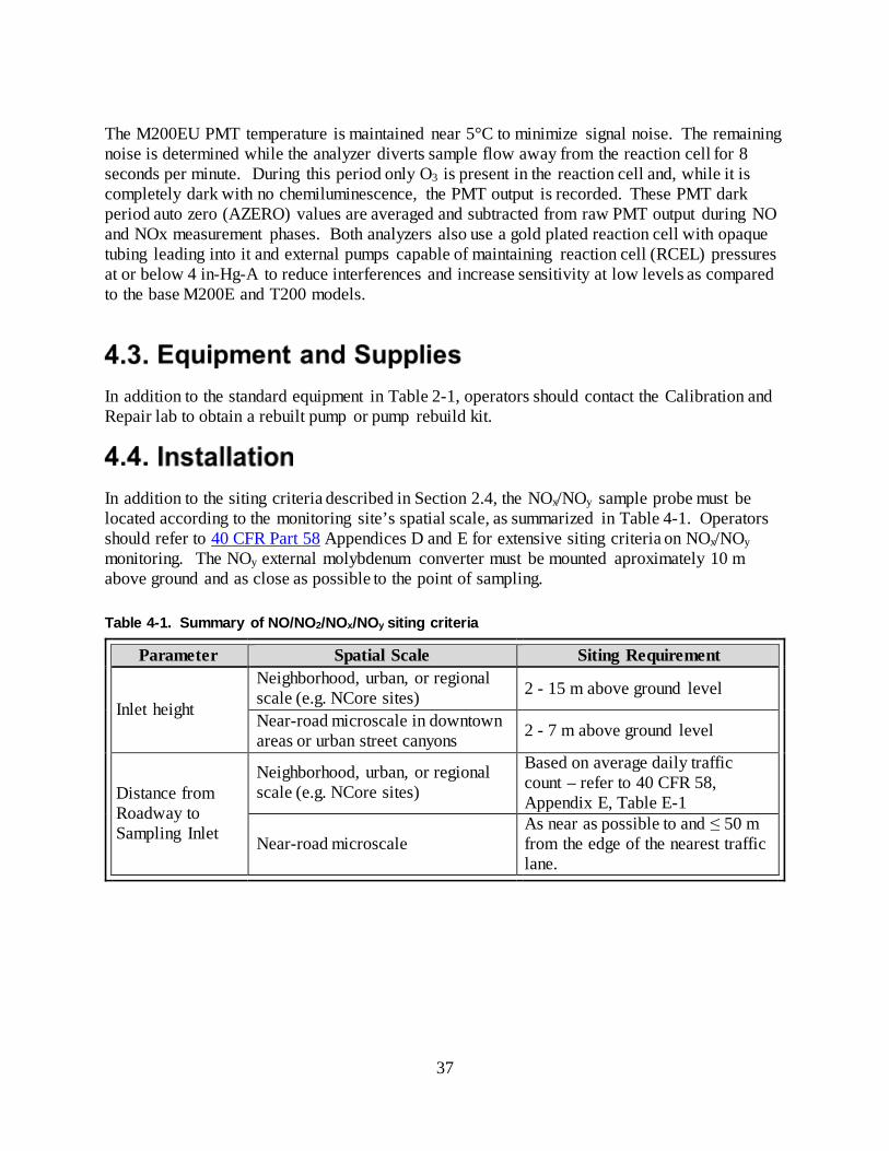
In addition to the siting criteria described in Section 2.4, the NOx/NOy sample probe must be located according to the monitoring site’s spatial scale, as summarized in Table 4-1. Operators should refer to 40 CFR Part 58 Appendices D and E for extensive siting criteria on NOx/NOy monitoring. The NOy external molybdenum converter must be mounted aproximately 10 m above ground and as close as possible to the point of sampling. Table 4-1. Summary of NO/NO2/NOx/NOy siting criteria

Parameter Spatial Scale Siting Requirement

Inlet height

Neighborhood, urban, or regional scale (e.g. NCore sites) 2 - 15 m above ground level

Near-road microscale in downtown areas or urban street canyons 2 - 7 m above ground level

Distance from Roadway to Sampling Inlet

Neighborhood, urban, or regional scale (e.g. NCore sites)

Based on average daily traffic count – refer to 40 CFR 58, Appendix E, Table E-1

Near-road microscale As near as possible to and ≤ 50 m from the edge of the nearest traffic lane.

http://www.ecfr.gov/cgi-bin/retrieveECFR?n=40y6.0.1.1.6

38

4.5.1. Quality Control Checks In addition to the procedures described in Section 2.5.1, operators must be particularly attentive to scheduling QC checks and maintenance to minimize data loss. Multi-point QC checks with a zero, three NO/NOx and two NO2 span points will require about 2.5 hours. An additional 3.5 hours of maintenance, QC checks or other down time on the same day could lead to failing to meet data completeness requirements for the entire day. The recommended action levels for recalibration are illustrated in Figure 4-1.

Figure 4-1. NO/NO2/NOx/NOy action levels for recalibration

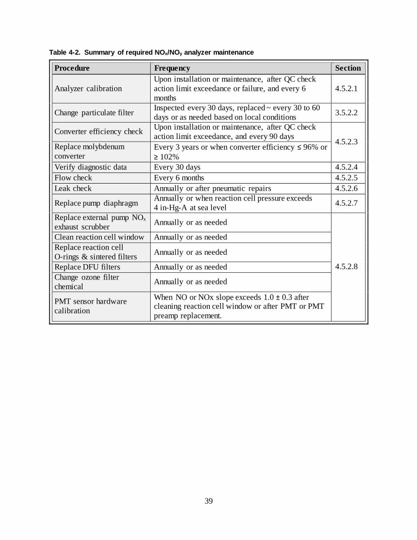
4.5.2. Maintenance The maintenance schedule for the Teledyne API M200EU analyzer is summarized in Table 4-2 below. The maintenance schedule for the T200U NOy is described in the TAPI T200U NOy addendum to the TAPI T200U manual. Other analyzers should be maintained according to their SOPs and associated requirements in their federal reference or equivalent method (FRM/FEM) designations. Additional questions regarding maintenance schedules should be directed to the Calibration and Repair Laboratory or Quality Assurance personnel.

39

Table 4-2. Summary of required NOx/NOy analyzer maintenance


Analyzer calibration Upon installation or maintenance, after QC check action limit exceedance or failure, and every 6 months

4.5.2.1

Change particulate filter Inspected every 30 days, replaced ~ every 30 to 60 days or as needed based on local conditions 3.5.2.2

Converter efficiency check Upon installation or maintenance, after QC check action limit exceedance, and every 90 days 4.5.2.3 Replace molybdenum

converter Every 3 years or when converter efficiency ≤ 96% or ≥ 102%

Verify diagnostic data Every 30 days 4.5.2.4 Flow check Every 6 months 4.5.2.5 Leak check Annually or after pneumatic repairs 4.5.2.6

Replace pump diaphragm Annually or when reaction cell pressure exceeds 4 in-Hg-A at sea level 4.5.2.7

Replace external pump NOx exhaust scrubber Annually or as needed

4.5.2.8

Clean reaction cell window Annually or as needed Replace reaction cell O-rings & sintered filters Annually or as needed

Replace DFU filters Annually or as needed Change ozone filter chemical Annually or as needed

PMT sensor hardware calibration

When NO or NOx slope exceeds 1.0 ± 0.3 after cleaning reaction cell window or after PMT or PMT preamp replacement.

40

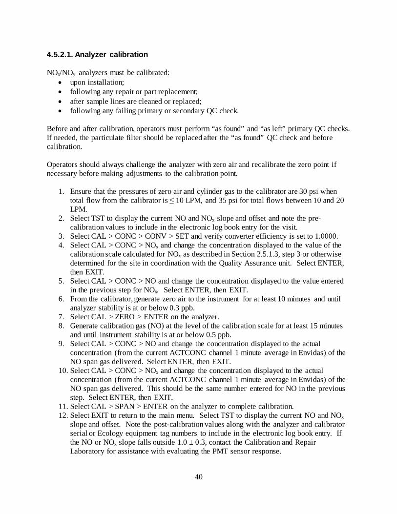
4.5.2.1. Analyzer calibration NOx/NOy analyzers must be calibrated:

• upon installation; • following any repair or part replacement; • after sample lines are cleaned or replaced; • following any failing primary or secondary QC check.

Before and after calibration, operators must perform “as found” and “as left” primary QC checks. If needed, the particulate filter should be replaced after the “as found” QC check and before calibration. Operators should always challenge the analyzer with zero air and recalibrate the zero point if necessary before making adjustments to the calibration point.

1. Ensure that the pressures of zero air and cylinder gas to the calibrator are 30 psi when total flow from the calibrator is ≤ 10 LPM, and 35 psi for total flows between 10 and 20 LPM.

2. Select TST to display the current NO and NOx slope and offset and note the pre-calibration values to include in the electronic log book entry for the visit.

3. Select CAL > CONC > CONV > SET and verify converter efficiency is set to 1.0000. 4. Select CAL > CONC > NOx and change the concentration displayed to the value of the

calibration scale calculated for NOx as described in Section 2.5.1.3, step 3 or otherwise determined for the site in coordination with the Quality Assurance unit. Select ENTER, then EXIT.

5. Select CAL > CONC > NO and change the concentration displayed to the value entered in the previous step for NOx. Select ENTER, then EXIT.

6. From the calibrator, generate zero air to the instrument for at least 10 minutes and until analyzer stability is at or below 0.3 ppb.

7. Select CAL > ZERO > ENTER on the analyzer. 8. Generate calibration gas (NO) at the level of the calibration scale for at least 15 minutes

and until instrument stability is at or below 0.5 ppb. 9. Select CAL > CONC > NO and change the concentration displayed to the actual

concentration (from the current ACTCONC channel 1 minute average in Envidas) of the NO span gas delivered. Select ENTER, then EXIT.

10. Select CAL > CONC > NOx and change the concentration displayed to the actual concentration (from the current ACTCONC channel 1 minute average in Envidas) of the NO span gas delivered. This should be the same number entered for NO in the previous step. Select ENTER, then EXIT.

11. Select CAL > SPAN > ENTER on the analyzer to complete calibration. 12. Select EXIT to return to the main menu. Select TST to display the current NO and NOx

slope and offset. Note the post-calibration values along with the analyzer and calibrator serial or Ecology equipment tag numbers to include in the electronic log book entry. If the NO or NOx slope falls outside 1.0 ± 0.3, contact the Calibration and Repair Laboratory for assistance with evaluating the PMT sensor response.

41

Note: The ZERO or SPAN buttons may not display during the zero or span calibration if the measured concentration is too different from the expected value. Refer to the manufacturer’s operation manual for more information. 4.5.2.2. Change particulate filter The particulate filter should be inspected every 30 days for signs of plugging or excess dirt. The particulate filter should be changed monthly or when the color has noticeably changed. Operators should wear gloves and take care not to touch the inside surfaces, including glass window, PTFE or Viton O-rings, or assembly body, as contamination may lower the accuracy of readings.



2. Place all of the NOx/NOy analyzer channels offscan in the data collection system and turn off the analyzer.

3. Open the front panel and unscrew the knurled retaining ring of the filter assembly. 4. Carefully remove the retaining ring, glass window, and PTFE O-ring. Use clean tweezers

to remove the filter element. 5. Replace the filter element, centering it in the bottom of the holder. 6. Reinstall the PTFE O-ring (notches face up), the glass cover, and the retaining ring in the

order shown in Figure 4-2. Hand tighten. Visually inspect the seal between the glass cover and the O-ring to ensure that it is tight.


If not, repeat the process above until the flow rate returns to a similar value.

42

9. When the flow and ambient NO/NO2/NOx/NOy concentrations have returned to pre-maintenance values, return the analyzer channels to on/okay status and note the maintenance in the electronic log book.

4.5.2.3. Converter Efficiency Check The converter efficiency should be checked upon installation, after maintenance and calibration, and at least quarterly. A QC check should always precede the converter efficiency check. If the results from the NO or NOx QC check performed immediately before performing the converter efficiency check are outside ± 2%, the analyzer should be recalibrated before performing the converter efficiency check. When the reported values from this basic check are < 0.9700 or > 1.0100, the NOx analyzer should be recalibrated and the converter efficiency test performed again. If the measured efficiency is still outside these action limits, the more detailed procedure described in the M200E and T200 manuals for evaluating the NO2 to NO converter performance should be followed. The efficiency must be between 0.9600 and 1.0200 (96% and 102%). When it falls outside this range, the converter must be replaced. Under normal conditions the molybdenum converter is expected to be replaced every three years. Refer to the manufacturer’s operation manual or contact the Calibration and Repair Laboratory for assistance with these procedures.

1. Ensure that the pressures of zero air and cylinder gas to the calibrator are 30 psi when total flow from the calibrator is ≤ 10 LPM, and 35 psi for total flows between 10 and 20 LPM.

2. Select TST to display the current NO and NOx slope and offset and note the pre-test values to include in the electronic log book entry for the visit.

3. Select CAL > CONC > CONV > SET and verify converter efficiency is set to 1.0000. 4. Select CAL > CONC > CONV > NO2 and change the concentration displayed to the

value of the calibration scale calculated for NO2 as described in Section 2.5.1.3, step 3 or otherwise determined for the site in coordination with the Quality Assurance unit. Select ENTER, then EXIT.

5. Place all of the NOx/NOy analyzer channels offscan in the data collection system. 6. From the calibrator, perform a gas phase titration to generate NO2 calibration gas at the

level of the calibration scale. 7. Select CAL > CONC > CONV > CAL, select TST to toggle to the stability display, and

wait for at least 30 minutes or until instrument stability is at or below 0.5 ppb. Select ENTER, then SET.

8. Note the calculated converter efficiency factor to include it in the electronic log book, then change the value back to 1.0000 and select ENTER, then EXIT.

9. Select EXIT to return to the main menu. From the calibrator, generate zero air to the instrument until there is a stable one minute at zero in the data collection system, then place the calibrator in STANDBY.

10. After the analyzer’s response has returned to ambient concentrations, place all analyzer channels back to on/okay status in the data collection system and note the converter efficiency value along with the analyzer and calibrator serial or Ecology equipment tag numbers in the electronic log book.

43

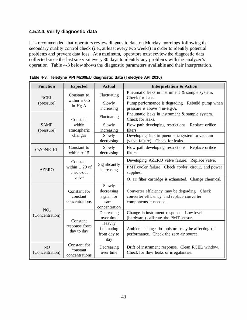
4.5.2.4. Verify diagnostic data It is recommended that operators review diagnostic data on Monday mornings following the secondary quality control check (i.e., at least every two weeks) in order to identify potential problems and prevent data loss. At a minimum, operators must review the diagnostic data collected since the last site visit every 30 days to identify any problems with the analyzer’s operation. Table 4-3 below shows the diagnostic parameters available and their interpretation. Table 4-3. Teledyne API M200EU diagnostic data (Teledyne API 2010)

Function Expected Actual Interpretation & Action

RCEL (pressure)

Constant to within ± 0.5

in-Hg-A

Fluctuating Pneumatic leaks in instrument & sample system. Check for leaks.

Slowly increasing

Pump performance is degrading. Rebuild pump when pressure is above 4 in-Hg-A.

SAMP (pressure)

Constant within

atmospheric changes

Fluctuating Pneumatic leaks in instrument & sample system. Check for leaks.

Slowly increasing

Flow path developing restrictions. Replace orifice filters.

Slowly decreasing

Developing leak in pneumatic system to vacuum (valve failure). Check for leaks.

OZONE FL Constant to within ± 15

Slowly decreasing

Flow path developing restrictions. Replace orifice filters.

AZERO

Constant within ± 20 of

check-out valve

Significantly increasing

Developing AZERO valve failure. Replace valve. PMT cooler failure. Check cooler, circuit, and power supplies. O3 air filter cartridge is exhausted. Change chemical.

NO2 (Concentration)

Constant for constant

concentrations

Slowly decreasing signal for

same concentration

Converter efficiency may be degrading. Check converter efficiency and replace converter components if needed.

Constant response from

day to day


Change in instrument response. Low level (hardware) calibrate the PMT sensor.

Heavily fluctuating

from day to day

Ambient changes in moisture may be affecting the performance. Check the zero air source.

NO (Concentration)

Constant for constant

concentrations


Drift of instrument response. Clean RCEL window. Check for flow leaks or irregularities.

44

4.5.2.5. Flow check In addition to reviewing the analyzer’s reported flow via diagnostics, operators should verify the analyzer’s flow every 6 months using a NIST-traceable flow meter certified to 1000 sccm.


that the inlet to the flow meter is at atmospheric pressure. 3. The sample flow measured with the external flow meter should be 1000 sccm ± 10%. 4. If needed, adjust the internal flow sensor according to the procedures in the instrument

manual. Low flows indicate that the pneumatic pathways may be blocked. Refer to the manufacturer’s manual or contact the Calibration and Repair Laboratory for troubleshooting assistance. 4.5.2.6. Leak check To perform an analyzer vacuum leak check and verify the pump condition:

1. Ensure the analyzer has warmed up for at least 30 minutes and the flows have stabilized. 2. Disconnect the inlet tubing and cap the analyzer port, wrench tight. 3. When the pressures are stable, note the SAMP (sample pressure) and RCEL (reaction cell

pressure) readings. a. If both readings are within 10% and < 4 in-Hg-A, the analyzer is free of large

leaks and the pump is acceptable. b. If the pressure is near or ≥ 4 in-Hg-A, the pump diaphragm should be replaced. c. If the readings exceed 10% difference, there is a leak that requires corrective

action and a detailed pressure leak check should be performed to identify the location of the leak and it must be repaired.

To perform a detailed pressure leak check, operators must pressurize the instrument to 10 psi and hold the pressure for about 10 minutes. This can be achieved with a hand-held pressure pump with pressure gauge or with a tank of pressured gas (ultrapure air or nitrogen) with a two-stage regulator adjusted to < 15 psi, a shutoff valve and a pressure gauge.



measures a loss exceeding 0.8 psi during that time, there is a leak in the pneumatics. 5. If the leak check fails, use a liquid leak detector (e.g. Snoop®) to search for leaks.


6. Reconnect the sample and exhaust lines and replace the instrument cover.

45

4.5.2.7. Replace pump diaphragm Low flow or no flow can be a sign of worn-out seals in the pump. Pumps must be rebuilt using the Teledyne API pump rebuild kit annually or more frequently as the RCEL pressure values approach 4 in-Hg-A. Detailed instructions are included with the rebuild kit. Always perform flow and leak checks after the pump is rebuilt. 4.5.2.8. Annual Maintenance and Repair Many of the required annual maintenance procedures are best performed in a laboratory environment; please contact the Calibration and Repair Laboratory to obtain parts and supplies and to coordinate annual maintenance items. Follow procedures in the applicable analyzer manuals for the following activities:

• replacing the external pump NOx exhaust scrubber • cleaning the reaction cell window • replacing reaction cell O-rings and sintered filters • replacing DFU filters • changing the ozone filter chemical • PMT sensor hardware calibration

There may be multiple manuals and applicable addenda for a particular analyzer. For example, the TAPI T200U NOy requires familiarity with the T200 manual and T200U and T200U NOy addenda and the M200EU requires the M200E manual and the M200EU addendum. Most procedures are described in the base version of the manual but requirements and parts specific to the high sensitivity models are described in the addenda, like the requirement for pumps to maintain less than 4 in-Hg-A in the reaction cell. Reading only the procedures in the M200E manual, an operator might mistakenly believe the pump doesn’t need to be rebuilt until the vacuum reaches 10 in-Hg-A. Some tasks may need to be performed more often than annually due to site-specific conditions or in response to other maintenance. Also, some items in Table 4-2 and Table 4-3 may require additional evaluation before performing recommended corrective actions. For example, if it has been several months since annual maintenance, cleaning the reaction cell may correct a slope exceeding specifications and a PMT hardware calibration may not be necessary or advised. Consult with the Calibration and Repair Laboratory for troubleshooting assistance.

46

4.6.1. Envidas Channel Configuration The correct configurations for NO/NO2/NOx concentration channels are shown in Figure 4-3 through Figure 4-5. Three data channels must be configured to record NO, NO2 and NOx concentrations in ppb for NAAQS compliance evaluation, to support modeling and other applications and for display on Ecology’s website.

Figure 4-3. NO channel configuration

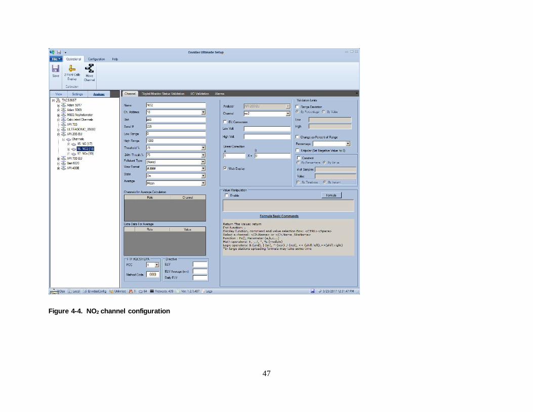
47

Figure 4-4. NO2 channel configuration

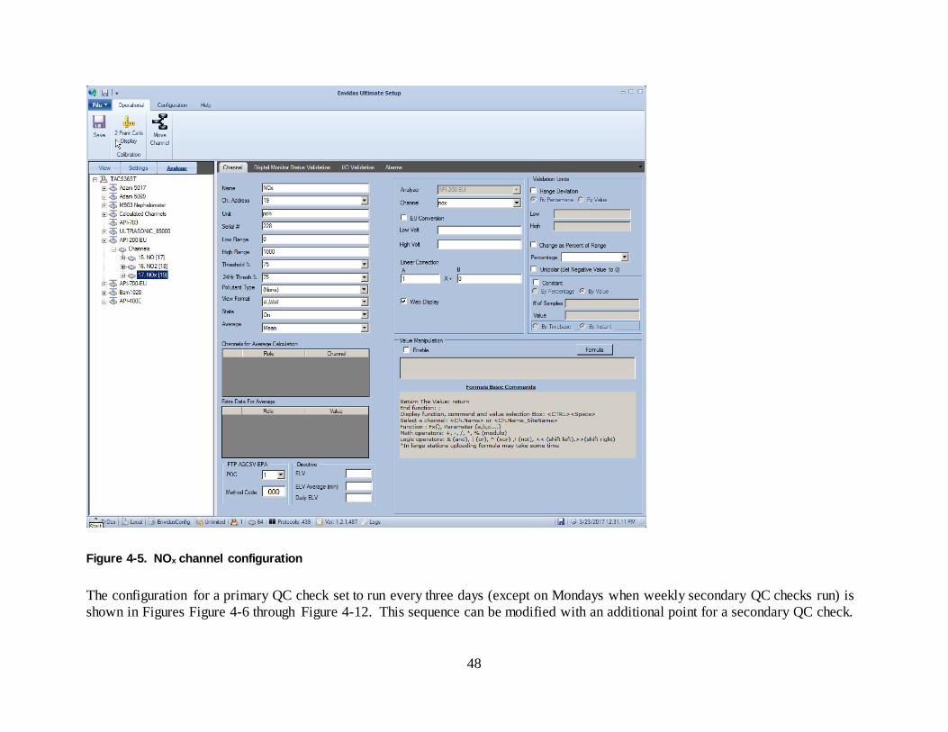
48

Figure 4-5. NOx channel configuration The configuration for a primary QC check set to run every three days (except on Mondays when weekly secondary QC checks run) is shown in Figures Figure 4-6 through Figure 4-12. This sequence can be modified with an additional point for a secondary QC check.

49

All NO/NOx phases should last a minimum of 15 minutes and NO2 gas-phase titration (GPT) phases should last a minimum of 30 minutes, not including gas phase titration pre-set (GPTPS) steps. For zero and NO/NOx points, the reference value should be a 2-minute NO/NOx channel average compared to the ACTCONC channel; this should not include the last minute of the phase. For NO2 points, the reference value is the target value the calibrator is set to deliver. This is compared to a 5-minute NO2 channel average that does not include the last minute of the phase. The example primary QC sequence shown combines NO, NOx and NO2 points with a single zero point and when assigned to all three channels, will flag the channels during the sequence. If separate QC sequences are used for NO/NOx versus NO2, the sequences must be configured to flag all three channels. NO2 span point GPT and GPTPS phases must be programmed into the site calibrator following procedures in this SOP and analyzer manual. The GPTPS step allows the calibrator to adjust the ozone generator lamp to the correct voltage more quickly during subsequent GPT steps under the same concentration and flow settings. A GPTPS using the same settings to be used in the sequence should be performed manually several times during initial setup of the calibrator for NO2 monitoring at the site. It will take about 20 - 30 minutes for the GPTPS to lock in the O3 value the first few times it is run. The calibrator should be preconditioned until it locks in the specified O3 value in the time set in the automated sequence, which is 8 minutes in the example below. These internal calibrator sequences are initiated by Envidas using the EXECSEQ command in the Envidas QC sequence. (Note that when using the EXECSEQ command in an Envidas sequence, the name of the sequence programmed into the calibrator must be placed in quotes, for example: C EXECSEQ “GPT40” as shown in the example sequences in the figures below.) In the Primary QC Check example, the following steps for the 40 ppb NO2 point are programmed into the 700EU in a sequence named GPT40:

1. GPTPS: 60 ppb NO, 40 ppb O3, 8 LPM 2. Duration: 8 min 3. GPT: 60 ppb NO, 40 ppb O3, 8 LPM 4. Duration 32 min 5. Standby

Also ensure that the default flow for the calibrator is set to the same value as used in the sequence to avoid settings conflicts.

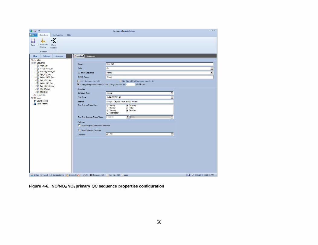
50

Figure 4-6. NO/NO2/NOx primary QC sequence properties configuration

51

Figure 4-7. NO/NO2/NOx primary QC sequence part 1

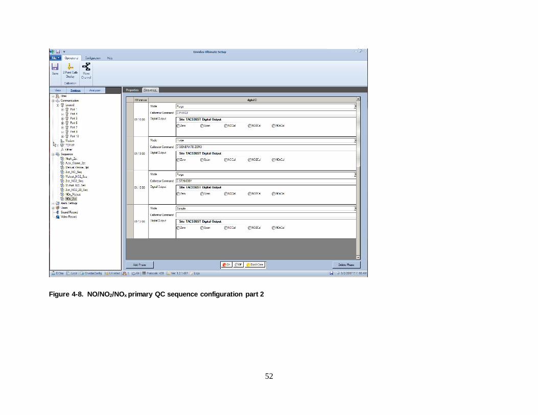
52

Figure 4-8. NO/NO2/NOx primary QC sequence configuration part 2

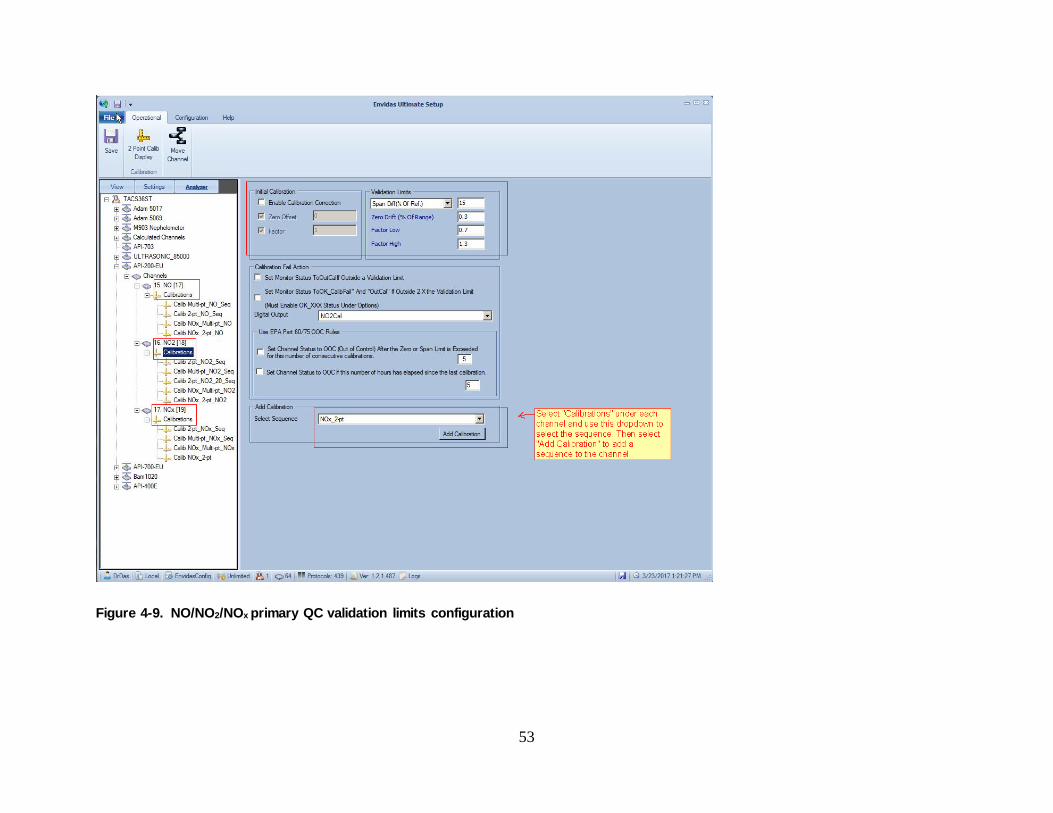
53

Figure 4-9. NO/NO2/NOx primary QC validation limits configuration

54

Figure 4-10. NO primary QC configuration of phases and reference values

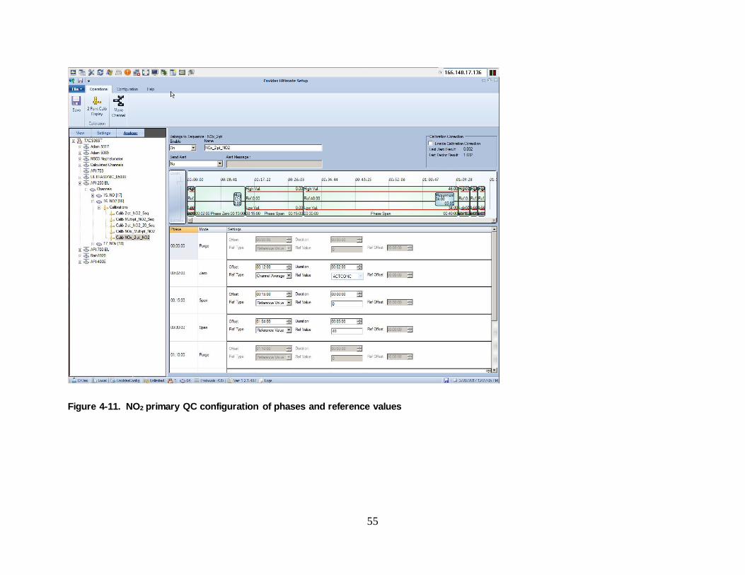
55

Figure 4-11. NO2 primary QC configuration of phases and reference values

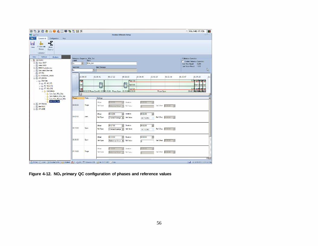
56

Figure 4-12. NOx primary QC configuration of phases and reference values

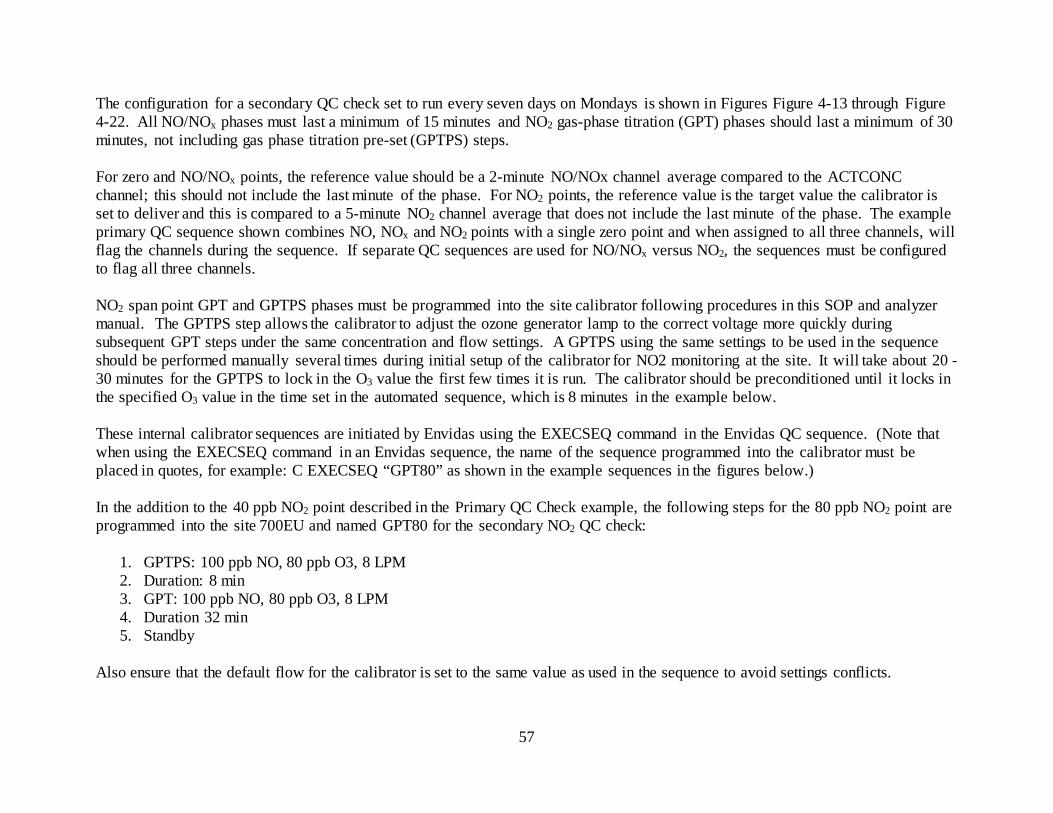
57

The configuration for a secondary QC check set to run every seven days on Mondays is shown in Figures Figure 4-13 through Figure 4-22. All NO/NOx phases must last a minimum of 15 minutes and NO2 gas-phase titration (GPT) phases should last a minimum of 30 minutes, not including gas phase titration pre-set (GPTPS) steps. For zero and NO/NOx points, the reference value should be a 2-minute NO/NOx channel average compared to the ACTCONC channel; this should not include the last minute of the phase. For NO2 points, the reference value is the target value the calibrator is set to deliver and this is compared to a 5-minute NO2 channel average that does not include the last minute of the phase. The example primary QC sequence shown combines NO, NOx and NO2 points with a single zero point and when assigned to all three channels, will flag the channels during the sequence. If separate QC sequences are used for NO/NOx versus NO2, the sequences must be configured to flag all three channels. NO2 span point GPT and GPTPS phases must be programmed into the site calibrator following procedures in this SOP and analyzer manual. The GPTPS step allows the calibrator to adjust the ozone generator lamp to the correct voltage more quickly during subsequent GPT steps under the same concentration and flow settings. A GPTPS using the same settings to be used in the sequence should be performed manually several times during initial setup of the calibrator for NO2 monitoring at the site. It will take about 20 - 30 minutes for the GPTPS to lock in the O3 value the first few times it is run. The calibrator should be preconditioned until it locks in the specified O3 value in the time set in the automated sequence, which is 8 minutes in the example below. These internal calibrator sequences are initiated by Envidas using the EXECSEQ command in the Envidas QC sequence. (Note that when using the EXECSEQ command in an Envidas sequence, the name of the sequence programmed into the calibrator must be placed in quotes, for example: C EXECSEQ “GPT80” as shown in the example sequences in the figures below.) In the addition to the 40 ppb NO2 point described in the Primary QC Check example, the following steps for the 80 ppb NO2 point are programmed into the site 700EU and named GPT80 for the secondary NO2 QC check:

1. GPTPS: 100 ppb NO, 80 ppb O3, 8 LPM 2. Duration: 8 min 3. GPT: 100 ppb NO, 80 ppb O3, 8 LPM 4. Duration 32 min 5. Standby

Also ensure that the default flow for the calibrator is set to the same value as used in the sequence to avoid settings conflicts.

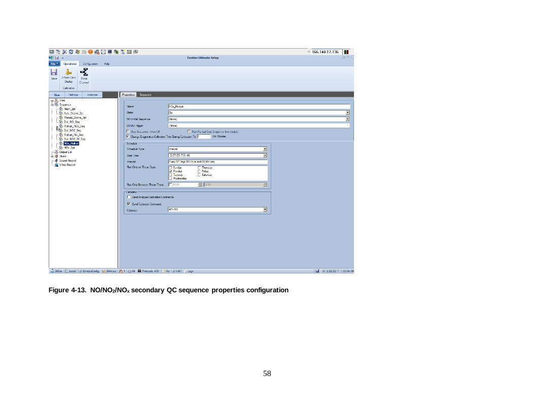
58

Figure 4-13. NO/NO2/NOx secondary QC sequence properties configuration

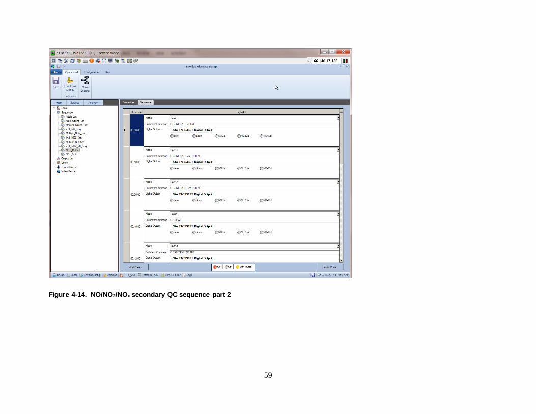
59

Figure 4-14. NO/NO2/NOx secondary QC sequence part 2

60


61


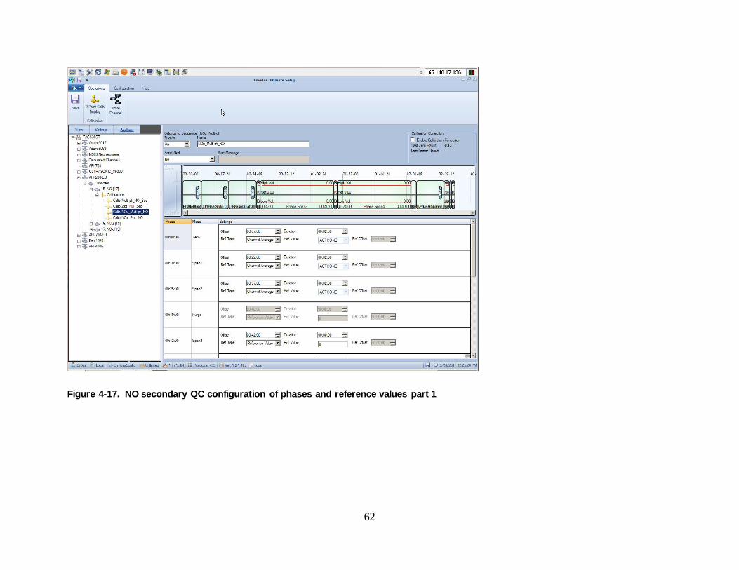
62

Figure 4-17. NO secondary QC configuration of phases and reference values part 1

63

Figure 4-18. NO secondary QC configuration of phases and reference values part 2

64

Figure 4-19. NO2 secondary QC configuration of phases and reference values part 1

65

Figure 4-20. NO2 secondary QC configuration of phases and reference values part 2

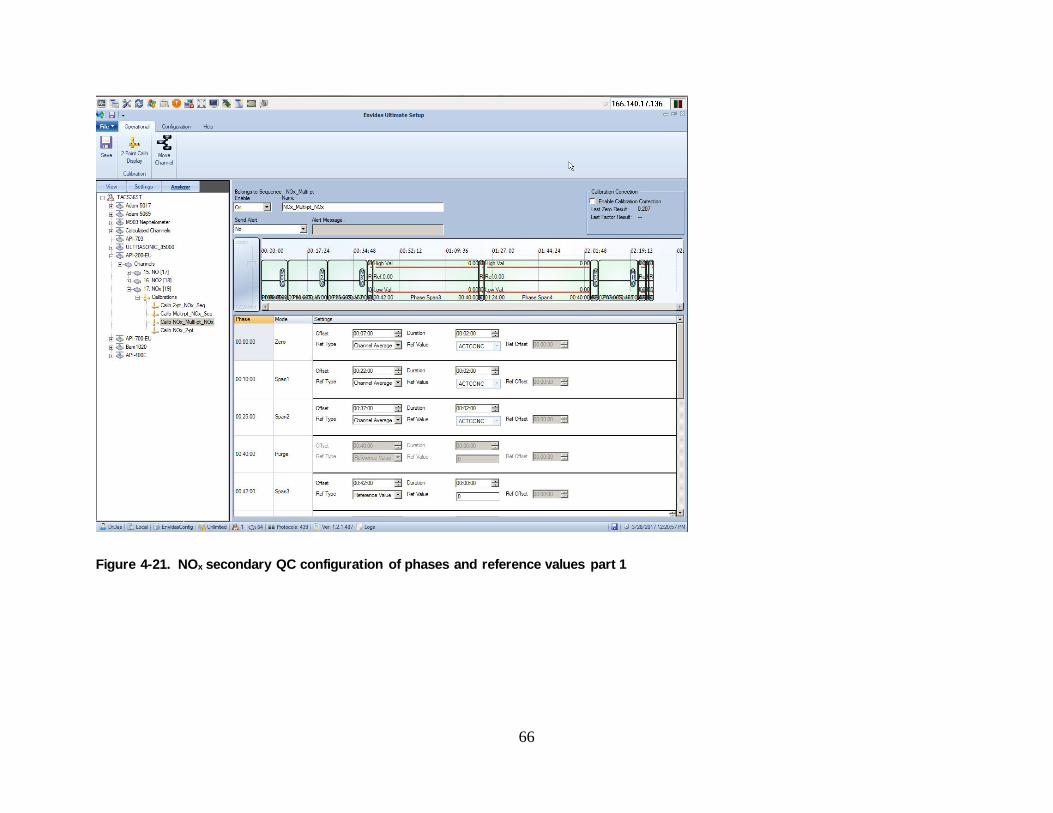
66

Figure 4-21. NOx secondary QC configuration of phases and reference values part 1

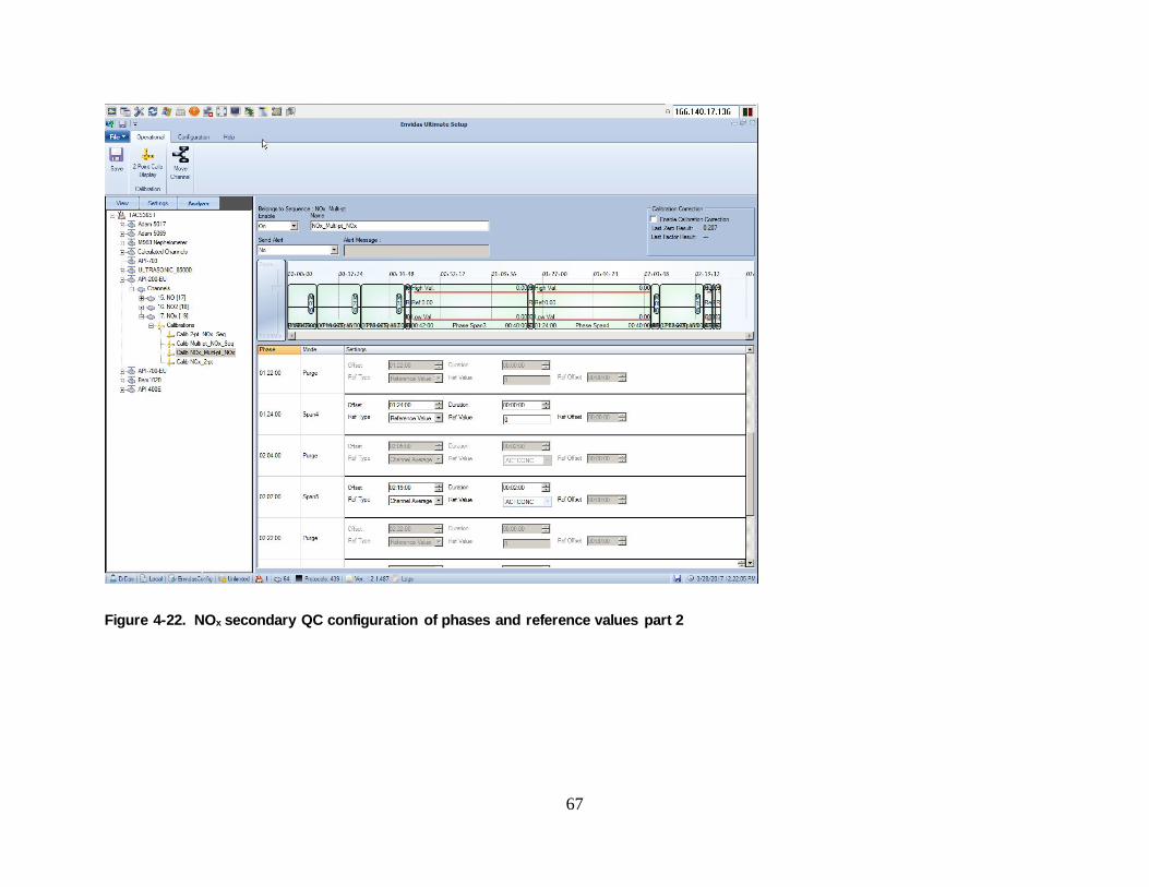
67

Figure 4-22. NOx secondary QC configuration of phases and reference values part 2

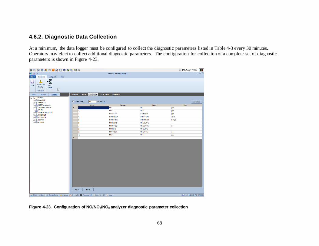
68

4.6.2. Diagnostic Data Collection At a minimum, the data logger must be configured to collect the diagnostic parameters listed in Table 4-3 every 30 minutes. Operators may elect to collect additional diagnostic parameters. The configuration for collection of a complete set of diagnostic parameters is shown in Figure 4-23.

Figure 4-23. Configuration of NO/NO2/NOx analyzer diagnostic parameter collection

69

Carbon Monoxide (CO) Monitoring

This chapter describes Ecology’s procedures for monitoring trace- and ambient-level CO concentrations using the Teledyne API T300U and T300 analyzers. It includes procedures for installation, operation, quality control, maintenance, and data acquisition. It is intended to be used with the manufacturer’s model-specific operation manual and Chapter 2, which describes general procedures for gaseous pollutant monitoring and calibration with dynamic dilution calibration systems.

The CO concentrations in the ambient air are measured based on the absorption of infrared radiation (IR) by CO. A source IR beam is passed into a sample chamber where mirrors reflect the light beam multiple times to achieve the intended levels of light intensity. Upon exiting the chamber, the beam is passed through a band-pass filter to only allow IR at a wavelength of 4.7 μm to reach a photometer. To overcome the measurement interference from gases such as water vapor and carbon dioxide that also absorb at this wavelength, the instrument uses Gas Filter Correlation (GFC) at the upstream of the sample chamber. The GFC Wheel consists of two semi-circle cells, one filled with pure nitrogen (N2) (measurement cell) and another filled with N2 and a high concentration of CO (reference cell). As the IR source passes through the spinning wheel and the sample air in the chamber, the alternating IR absorption capacities in the two cells create pulses of measurement peak (CO MEAS) and reference peak (CO REF) since N2 does not absorb any IR. The ratio of CO MEAS to CO REF, or M/R ratio, can thus be calculated. If interfering gas is present in the sample chamber, it only reduces the IR signals the same way in both measurement and reference cells while the M/R ratio stays unchanged. As a result, GFC rejects the effects of interfering gases and the analyzer only responds to the CO in the sample air. Once the M/R ratio is obtained, the analyzer uses an internal look-up table to interpolate the reading and applies calibration (slope and offset) to calculate the final CO concentrations. The primary difference between the trace-level analyzers (300EU and T300U) and the ambient-level ones (300E and T300) is the use of auto-reference (A-REF) ratio and the Nafion® dryer. The A-REF ratio is used to correct drift caused by the aging photometer components (e.g. IR lamp, IR detector, etc.), variation in ambient temperature and interfering gases. It is derived in the same way as the M/R ratio, except that the air sample is routed to a CO scrubber prior to entering the sample chamber, so the difference between CO MEAS and CO REF represents the exact state of the sample gas and the photometer component free of CO. A-REF cycle is triggered every 4 hours by the analyzer and takes approximately 15 minutes. After the cycle, the analyzer averages the last five A-REF ratios and applies the value in the final CO calculation as an offset. The Nafion® dryer is located upstream of the CO scrubber and consists of a bundle of

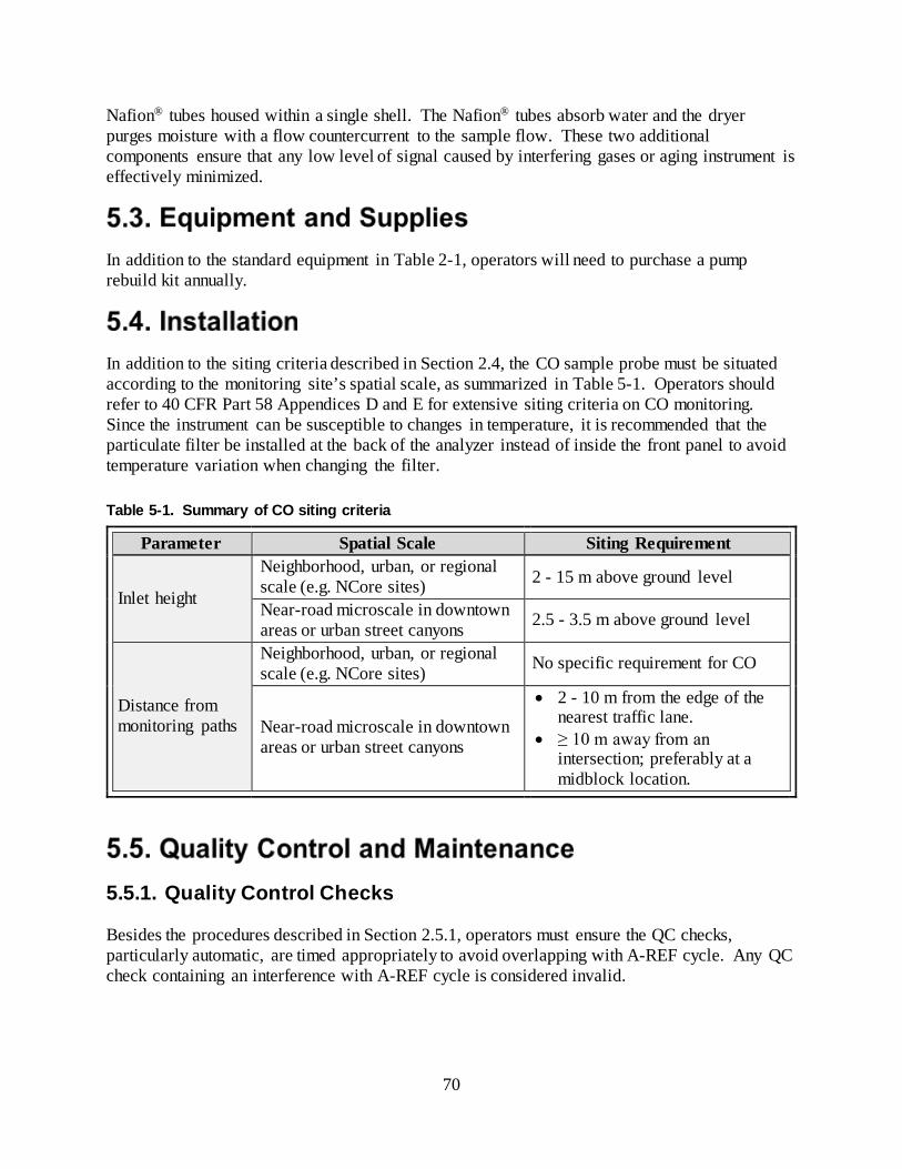
70

Nafion® tubes housed within a single shell. The Nafion® tubes absorb water and the dryer purges moisture with a flow countercurrent to the sample flow. These two additional components ensure that any low level of signal caused by interfering gases or aging instrument is effectively minimized.

In addition to the standard equipment in Table 2-1, operators will need to purchase a pump rebuild kit annually.

In addition to the siting criteria described in Section 2.4, the CO sample probe must be situated according to the monitoring site’s spatial scale, as summarized in Table 5-1. Operators should refer to 40 CFR Part 58 Appendices D and E for extensive siting criteria on CO monitoring. Since the instrument can be susceptible to changes in temperature, it is recommended that the particulate filter be installed at the back of the analyzer instead of inside the front panel to avoid temperature variation when changing the filter. Table 5-1. Summary of CO siting criteria

Parameter Spatial Scale Siting Requirement

Inlet height

Neighborhood, urban, or regional scale (e.g. NCore sites) 2 - 15 m above ground level

Near-road microscale in downtown areas or urban street canyons 2.5 - 3.5 m above ground level

Distance from monitoring paths

Neighborhood, urban, or regional scale (e.g. NCore sites) No specific requirement for CO

Near-road microscale in downtown areas or urban street canyons

• 2 - 10 m from the edge of the nearest traffic lane.

• ≥ 10 m away from an intersection; preferably at a midblock location.

5.5.1. Quality Control Checks Besides the procedures described in Section 2.5.1, operators must ensure the QC checks, particularly automatic, are timed appropriately to avoid overlapping with A-REF cycle. Any QC check containing an interference with A-REF cycle is considered invalid.

71

The recommended action levels for recalibration are illustrated in Figure 5-1.

Figure 5-1. CO action levels for recalibration

5.5.2. Maintenance The maintenance schedule for the Teledyne API 300U and T300U CO analyzers is summarized in Table 5-2. Table 5-2. Summary of required CO analyzer maintenance


Analyzer calibration Upon installation or maintenance, after QC check failure, and every 6 months 3.5.2.1

Change particulate filter Every 30 days or as needed 3.5.2.2 Verify diagnostic data Every 30 days 3.5.2.4 Flow check Every 6 months 3.5.2.5 Pressure leak check Annually or after pneumatic repairs 3.5.2.6

Replace pump diaphragm Annually or when reaction cell pressure exceeds 4 in-Hg-A at sea level 4.5.2.7

50

- 50

30

- 30

7

- 7

10

- 7 - 10

72

5.5.2.1. Analyzer calibration CO analyzers must be calibrated:

• upon installation; • following any repair or part replacement; • after sample lines are cleaned or replaced; • following any failing primary or secondary QC check.

Before and after calibration, operators must perform “as found” and “as left” primary QC checks. Operators should always challenge the analyzer with zero air and recalibrate the zero point if necessary before making adjustments to the calibration point.

1. Ensure that the pressures of zero air and cylinder gas to the calibrator are between 25 and 30 psi.

2. Select CAL > CONC and change the concentration displayed to the value of the calibration scale (see Section 2.5.1.3). Select ENTER, then EXIT.

3. From the calibrator, generate zero air to the instrument for at least 30 minutes or until analyzer stability is at or below 10 ppb for trace-level CO.

4. Select CAL > ZERO > ENTER on the analyzer. 5. Generate calibration gas at the level of the calibration scale for at least 30 minutes or until

instrument stability is at or below 10 ppb for trace-level CO. 6. Select CAL > SPAN > ENTER on the analyzer to complete calibration. 7. Select EXIT to return to the main menu.

Note: The ZERO or SPAN buttons may not display during the zero or span calibration if the measured concentration is too different from the expected value. Refer to the manufacturer’s operation manual for more information. 5.5.2.2. Change particulate filter The particulate filter should be inspected every 30 days for signs of plugging or excess dirt. The particulate filter should be changed monthly or when the color has noticeably changed. Operators should wear gloves and take care not to touch the glass window with bare hands, as contamination may lower the accuracy of readings.

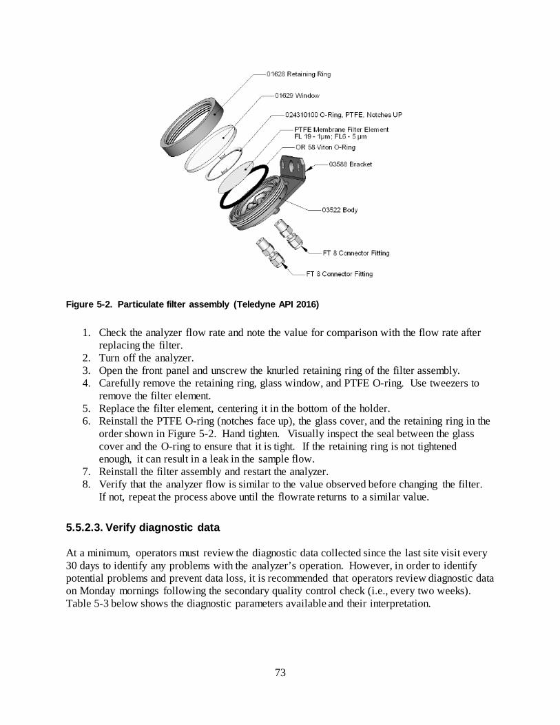
73



2. Turn off the analyzer. 3. Open the front panel and unscrew the knurled retaining ring of the filter assembly. 4. Carefully remove the retaining ring, glass window, and PTFE O-ring. Use tweezers to

remove the filter element. 5. Replace the filter element, centering it in the bottom of the holder. 6. Reinstall the PTFE O-ring (notches face up), the glass cover, and the retaining ring in the

order shown in Figure 5-2. Hand tighten. Visually inspect the seal between the glass cover and the O-ring to ensure that it is tight. If the retaining ring is not tightened enough, it can result in a leak in the sample flow.


If not, repeat the process above until the flowrate returns to a similar value. 5.5.2.3. Verify diagnostic data At a minimum, operators must review the diagnostic data collected since the last site visit every 30 days to identify any problems with the analyzer’s operation. However, in order to identify potential problems and prevent data loss, it is recommended that operators review diagnostic data on Monday mornings following the secondary quality control check (i.e., every two weeks). Table 5-3 below shows the diagnostic parameters available and their interpretation.

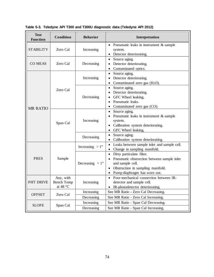
74

Table 5-3. Teledyne API T300 and T300U diagnostic data (Teledyne API 2012)

Test Function Condition Behavior Interpretation

STABILITY

Zero Cal Increasing

• Pneumatic leaks in instrument & sample system.

• Detector deteriorating.

CO MEAS Zero Cal Decreasing • Source aging. • Detector deteriorating. • Contaminated optics.

MR RATIO

Zero Cal

Increasing • Source aging. • Detector deteriorating. • Contaminated zero gas (H2O).

Decreasing

• Source aging. • Detector deteriorating. • GFC Wheel leaking. • Pneumatic leaks. • Contaminated zero gas (CO).

Span Cal

Increasing

• Source aging. • Pneumatic leaks in instrument & sample

system. • Calibration system deteriorating. • GFC Wheel leaking.

Decreasing • Source aging. • Calibration system deteriorating.

PRES Sample

Increasing > 1” • Leaks between sample inlet and sample cell. • Change in sampling manifold.

Decreasing > 1”

• Dirty particulate filter. • Pneumatic obstruction between sample inlet

and sample cell. • Obstruction in sampling manifold. • Pump diaphragm has worn out.

PHT DRIVE Any, with

Bench Temp at 48 °C

Increasing • Poor mechanical connection between IR-

detector and sample cell. • IR-photodetector deteriorating.

OFFSET Zero Cal Increasing See MR Ratio - Zero Cal Decreasing. Decreasing See MR Ratio - Zero Cal Increasing.

SLOPE Span Cal Increasing See MR Ratio - Span Cal Decreasing. Decreasing See MR Ratio - Span Cal Increasing.

75

5.5.2.4. Flow check In addition to reviewing the analyzer’s reported flow via diagnostics, operators should verify the analyzer’s flow every 6 months using a certified, NIST-traceable flow meter. The external flow device should be capable of measuring flows between 0 and 1000 sccm. Do not use the flow measurement displayed on the front panel for this flow check.


that the inlet to the flow meter is at atmospheric pressure. 3. The sample flow measured with the external flow meter should be 800 sccm ± 10%. 4. If needed, adjust the internal flow sensor following the procedures in the instrument

manual. Low flows indicate that the pneumatic pathways are blocked. Refer to the manufacturer’s operation manual or contact the Calibration and Repair Laboratory for troubleshooting assistance. 5.5.2.5. Leak check To perform a leak check, operators must pressurize the instrument to 10 psi and hold the pressure for about 10 minutes. This can be achieved with a hand-held pressure pump with pressure gauge or with a tank of pressured gas (ultrapure air or nitrogen) with a two-stage regulator adjusted to < 15 psi, a shutoff valve and a pressure gauge.



measures a loss exceeding 0.8 psi during that time, the pneumatics have a leak. 5. If the leak check fails, use a liquid leak detector (e.g. Snoop®) to search for leaks.


6. Reconnect the sample and exhaust lines, and replace the instrument cover. 5.5.2.6. Replace pump diaphragm Normal sample pressure is 29.92 in-Hg at sea level. Actions should be taken if pressure reading is < 10 in-Hg or > 35 in-Hg (see “PRES” in Table 5-3). A simple pump check can be performed prior to pump replacement following instructions in the operation manual. Low flow or no flow can be a sign of worn-out seals in the pump. Pumps must be rebuilt using the Teledyne API pump rebuild kit annually or more frequently as the RCEL pressure values approach 4 in-Hg-A.

76

Detailed instructions are included with the rebuild kit. Always perform flow and leak check after the pump is rebuilt.

5.6.1. Envidas Channel Configuration The correct configuration for CO concentration channels is shown in Figure 5-3 and Figure 5-4. Two channels must be set up to record CO concentrations in ppb for NAAQS compliance purposes (Figure 5-3) and in ppm for WAQA display on the Ecology web page (Figure-4).

Figure 5-3. CO channel configuration for NAAQS compliance

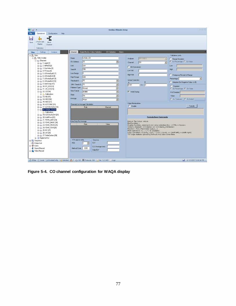
77

Figure 5-4. CO channel configuration for WAQA display

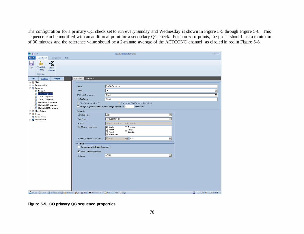
78

The configuration for a primary QC check set to run every Sunday and Wednesday is shown in Figure 5-5 through Figure 5-8. This sequence can be modified with an additional point for a secondary QC check. For non-zero points, the phase should last a minimum of 30 minutes and the reference value should be a 2-minute average of the ACTCONC channel, as circled in red in Figure 5-8.

Figure 5-5. CO primary QC sequence properties

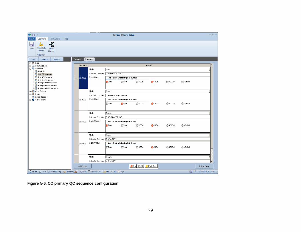
79

Figure 5-6. CO primary QC sequence configuration

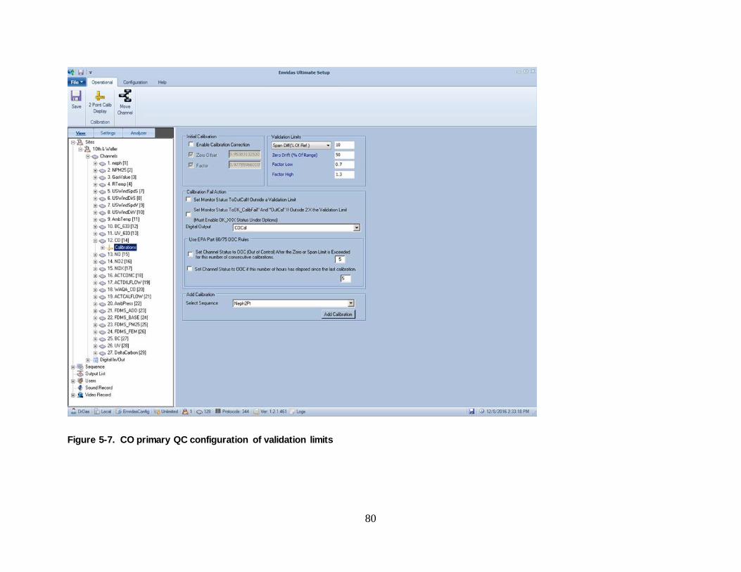
80

Figure 5-7. CO primary QC configuration of validation limits

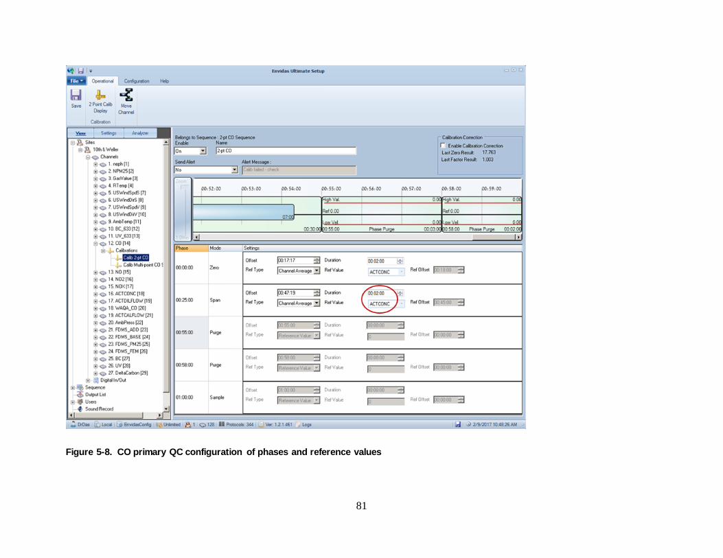
81

Figure 5-8. CO primary QC configuration of phases and reference values

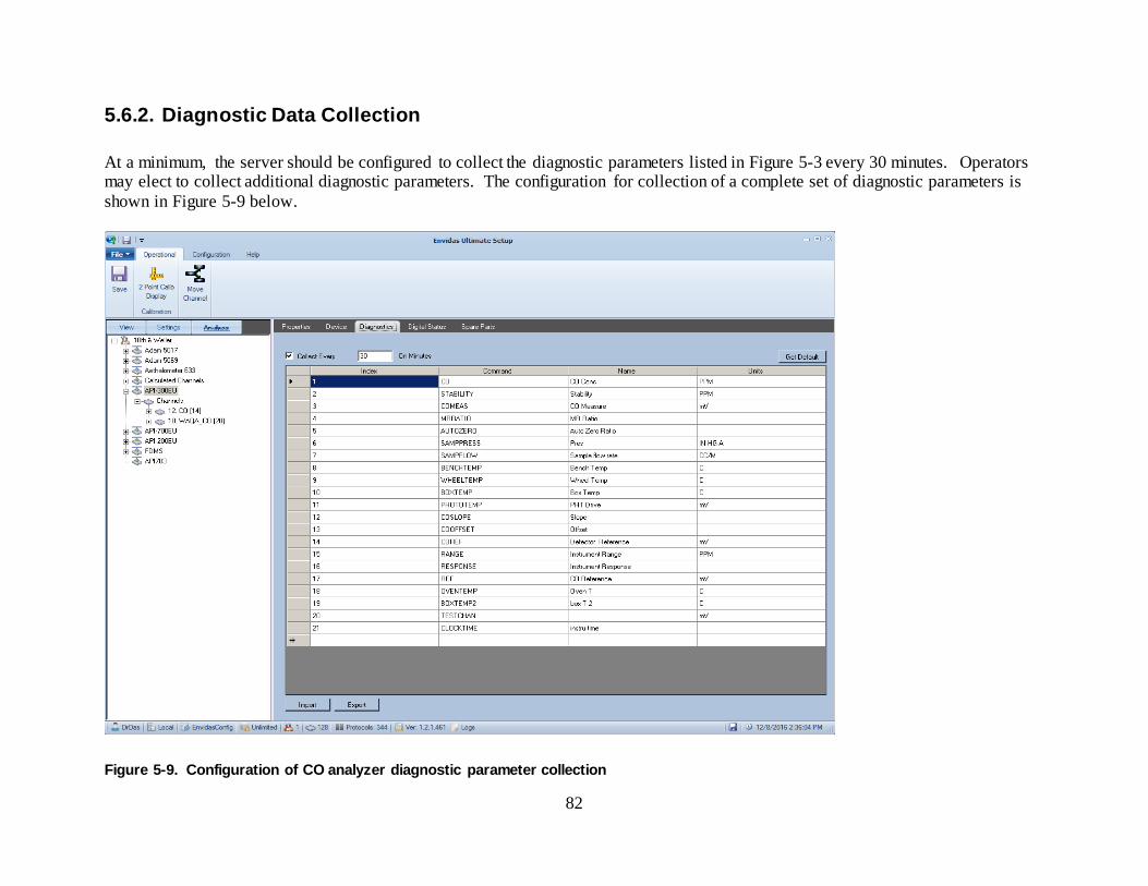
82

5.6.2. Diagnostic Data Collection At a minimum, the server should be configured to collect the diagnostic parameters listed in Figure 5-3 every 30 minutes. Operators may elect to collect additional diagnostic parameters. The configuration for collection of a complete set of diagnostic parameters is shown in Figure 5-9 below.

Figure 5-9. Configuration of CO analyzer diagnostic parameter collection

83

References

“Ambient Air Monitoring Reference and Equivalent Methods” Code of Federal Regulations Title 40, Pt. 53, 2017 ed.

“Interpretation of the Primary National Ambient Air Quality Standards for Oxides of Nitrogen

(Nitrogen Dioxide)” Code of Federal Regulations Title 40, Pt. 50, Appendix S, 2017 ed. “Measurement Principle and Calibration Procedure for the Measurement of Nitrogen Dioxide in

the Atmosphere (Gas Phase Chemiluminescence)” Code of Federal Regulations Title 40, Pt. 50, Appendix F, 2017 ed.

“National primary and secondary ambient air quality standards for oxides of nitrogen (with

nitrogen dioxide as the indicator)” Code of Federal Regulations Title 40, Pt. 50.11, 2017 ed. “Network Design Criteria for Ambient Air Quality Monitoring” Code of Federal Regulations

Title 40, Pt. 58, Appendix D, 2017 ed. “Probe and Monitoring Path Siting Criteria for Ambient Air Quality Monitoring.” Code of

Federal Regulations Title 40, Pt. 58, Appendix E, 2017 ed. “Quality Assurance Requirements for Monitors used in Evaluations of National Ambient Air

Quality Standards.” Code of Federal Regulations Title 40, Pt. 58, Appendix A, 2016 ed. State of Alaska Department of Environmental Conservation. Division of Air Quality. Standard

Operating Procedures for Sulfur Dioxide (SO2) Monitoring by Ultraviolet Fluorescence. Anchorage, 2012 (Revision 2).

** Teledyne API’s manuals and addenda listed below are sorted by the instrument type, then by

year Teledyne API (2014). Operation Manual: Models T701, T701H, 701, and 701H Zero Air

Generators. San Diego, 2014. Teledyne API (2011). Operation Manual: Model 701 Zero Air Generator. San Diego, 2011. Teledyne API (2010). Operation Manual: Model 701H High Performance Zero Air Generator.

San Diego, 2010. Teledyne API (2009). Addendum for Model 701H Zero Air Module with Internal Dewpoint

Sensor. San Diego, 2009. Teledyne API (2015). Operation Manual: Model T700 Dynamic Dilution Calibrator. San Diego,

2015.

84

Teledyne API (2015). Addendum: Model T700U Calibrator. San Diego, 2015. Teledyne API (2015). Manual Addendum: Model 700EU Calibrator. San Diego, 2015. Teledyne API (2009). Operator’s Manual: Model 700E Dynamic Dilution Calibrator. San Diego,

2009. Teledyne API (2016). Operation Manual: Model T100 UV Fluorescence SO2 Analyzer. San

Diego, 2016. Teledyne API (2011). Operation Manual: Model 100E UV Fluorescence SO2 Analyzer. San

Diego, 2011. Teledyne API (2011). Addendum: Model T100U Trace Level UV Fluorescence SO2 Analyzer.

San Diego, 2011. Teledyne API (2009). Addendum: Model 100EU Trace Level SO2 Analyzer-Addendum. San

Diego, 2009. Teledyne API (2015). Operation Manual: Model T200 NO/NO2/NOx Analyzer. San Diego, 2015. Teledyne API (2013). Manual Addendum: Ultra Sensitivity Model T200U NO/NO2/NOx

Analyzer. San Diego, 2013. Teledyne API (2013). Addendum: T200U NOy Analyzer. San Diego, 2013. Teledyne API (2010). Technical Manual: Model 200E Nitrogen Oxide Analyzer. San Diego,

2010. Teledyne API (2010). Manual Addendum: Ultra Sensitivity Model M200EU NO/NO2/NOx

Analyzer. San Diego, 2010. Teledyne API (2010). Addendum: M200EU-NOy Converter. San Diego, 2010. Teledyne API (2012). Operation Manual: Model T300 Gas Filter Correlation CO Analyzer. San

Diego, 2012. Teledyne API (2012). Manual Addendum: Model T300U Ultra-Sensitive Gas Filter Correlation

CO Analyzer. San Diego, 2012. Teledyne API (2011). Operation Manual: Model 300E/EM CO Analyzer. San Diego, 2011. Teledyne API (2008). Operation Addendum: Model 300EU CO Analyzer. San Diego, 2008.

85

U.S. Environmental Protection Agency (2016). National Exposure Research Laboratory. List of Designated Reference and Equivalent Methods. Research Triangle Park, 2016 (https://www3.epa.gov/ttn/amtic/criteria.html).

U.S. Environmental Protection Agency (2013). Office of Air Quality Planning and Standards.

Quality Assurance Handbook for Air Pollution Measurement Systems Volume II: Ambient Air Quality Monitoring Program. Research Triangle Park, 2013 (EPA-454/B-13-003).

U.S. Environmental Protection Agency (2012). National Risk Management Research Laboratory.

EPA Traceability Protocol for Assay and Certification of Gaseous Calibration Standards. Research Triangle Park, 2012 (EPA-600/R-12/531).


Near-road NO2 Monitoring Technical Assistance Document. Research Triangle Park, 2012 (EPA-454/B-12-002).


Technical Assistance Document (TAD) for Precursor Gas Measurements in the NCore Multi-Pollutant Monitoring Network, version 4. Research Triangle Park, 2005 (EPA-454/R-05-003).

gaseous pollutant monitoring standard operating procedure ... · gaseous pollutant monitoring...

Documents