Stefanie Alki Delichatsios Professor Neil Gershenfeld

MAS.862 May 22, 2006

GA Optimization for RFID Broadband Antenna Applications

Abstract This paper examines genetic algorithm optimizers in antenna design. Specifically, we evaluate whether GA optimizers are appropriate design techniques for RFID broadband antenna design by looking at current research with GA antennas and deducing whether similar optimizers can be applied to RFID broadband antennas such as bowtie designs. 1 Introduction Passive Radio Frequency Identification (RFID) is a track and trace technology that has become increasingly popular for identifying objects throughout the supply chain [1]. The RFID transaction begins when a reader transmits energy to a tag. The transponder or tag, composed of an antenna and a microchip, is attached to an object and backscatters the object’s identification code back to the reader, which then processes the information and performs some action. Figure 1 displays the RFID system and its basic components and operating principles.

Figure 1. The RFID System and its basic components and operating principles.

A passive tag has no onboard power supply and instead operates on the power radiated by the reader antenna, allowing the tag to be small and disposable. In a packaging environment, tags can be affixed to pallets, cases, or individual items, facilitating inventory and reducing shrinkage for retailers and manufacturers.

Central Processing

Unit Reader Reader

Antenna

Operating Frequency 915 Mhz in US

Tag

Tag Antenna

Tag antenna backscatters tag’s identifier back to reader

Reader transmits electromagnetic energy to tag

OBJECT (I.e. case, pallet)

1.1 Challenges in RFID Antenna Design The success of an RFID system relies heavily on the efficiency of the tag antenna due to power, size, and cost constraints. Though Ultra-High Frequency (UHF) RFID has become the standard in supply chain tracking for its fast response rates and long read ranges, UHF antennas suffer limitations and their design poses many challenges. They are orientation-sensitive, radiating well in some directions and not at all in others; they are material-sensitive, penetrating easily through radiolucent materials but not at all through conductive or liquid materials; and they are narrowband, functioning over a limited range of frequencies. Orientation sensitivity is problematic in warehouse environments where tagged boxes are moving on conveyor belts, fork lifts, and other dynamic devices. As tagged objects get shifted, flipped, and rotated, the orientation of the RFID tag including the antenna likewise changes. Similarly, material-sensitivity creates an issue as many manufactured products, even a box of toothpaste, have some amount of foil lining that degrades the efficiency of the tag antenna. Bandwidth is another sensitivity that requires attention because UHF RFID systems operate at different frequencies around the world. While 915 Mhz is the UHF RFID standard in the United States, systems in Europe run at 867 Mhz, and systems in Japan operate at around 960 Mhz. EPCglobal, a global body for creating industry standards in RFID technology, requires UHF tags to operate between 860-960 Mhz as part of its latest Generation 2 standard [2]. That way, a tagged product manufactured in China can be shipped to the United States and continue to be identified and tracked. Existing tag antennas are designed for specific applications. For instance, the Albano-Dipole antenna is a three-dimensional folded dipole design that wraps around the corner of a box and is optimized to radiate omnidirectionally [3]. Despite its near omnidirectional functionality, the Albano-Dipole design does not perform well in the presence of metal and has a fairly limited bandwidth, 900 Mhz – 930 Mhz. Another tag antenna example is the Albano-Patch antenna, which again is a three-dimensional patch antenna that wraps around the corner of a box and radiates omnidirectionally and performs well in the presence of metal. Despite the positive attributes of the Albano-Patch antenna, its downfalls are its big size and cost and its narrow bandwidth. Both the Albano-Dipole antenna and the Albano-Patch antenna were designed using traditional antenna techniques and tricks and running endless simulations using High Frequency Structure Simulator (HFSS), a 3D electromagnetic field simulator based on Finite Elements Method (FEM) [4]. Since 1886, when Hertz experimentally showed that a current-carrying element creates electromagnetic radiation, antenna design has evolved from a simple dipole antenna to antennas of all shapes, sizes, and dimensions [5]. Nonetheless, antenna design remains a

challenging and enigmatic feat. Beyond simple straight wire antennas and arrays of those wire antennas, mathematical calculations become very complicated very quickly. Normally, an antenna designer will start with a known antenna and manipulate physical parameters such as antenna material and antenna size to optimize a particular antenna parameter such as bandwidth. This evolution of antenna design using intuition, empirical testing, and a bit of luck, leads to functioning but imprecise antennas. The attempt to create an “optimal” and precise antenna using traditional techniques is near impossible. Even using search optimizers such as conjugate gradient, Newton, and Simplex to optimize an antenna is not guaranteed because such techniques are local optimizers [6]. These techniques search for local extrema in a solution set by differentiating functions around a set of initial conditions. However, for a system whose solution space has many local maxima, these optimizing techniques are not ideal because they converge to local maxima instead of global maxima. 1.2 Genetic Algorithms A Genetic Algorithm (GA) search optimizer is a global optimizer that searches the entire solution space in a parallel fashion and does not rely on an initial set of conditions. GA optimizers are robust and perform well with discontinuous and non-differentiable functions where traditional local optimizers fail. The concept of GAs was brought to light by John Holland in 1975 with the publication of Adaptation in Natural and Artificial Systems and since then, GAs have been implemented in numerous applications ranging from code-breaking to circuit design to finance [7]. Genetic Algorithms entered the electromagnetic domain in the 1990s, and significant research has been done using GAs in antenna design [8]. Despite their simplistic appeal, the question remains, are genetic algorithms better suited for antenna design than existing design techniques? Do they offer something extra that existing methods don’t? Though literature on GAs and antenna design exists, there is barely any research on the application of GAs in RFID antenna design. In this paper, I survey existing projects that employ genetic algorithms for antenna design, specifically broadband antenna design, and compare the results to traditional broadband antennas, such as bowtie antennas. After analysis, I will declare my recommendation on whether or not to apply GAs to RFID antenna design. In Section 2, we begin with an introduction to antenna theory and design. We then explain genetic algorithms more deeply in Chapter 3. In Chapter 4, we survey seven antenna designs that people have developed using genetic algorithms. Finally in Chapter 5, we Acompare GA antennas to traditional antennas and deduce whether or not GA optimizers are appropriate for antenna design, and specifically RFID broadband antenna design.

2 Antenna Theory and Design An antenna is a "transition device, or transducer, between a guided wave and a free-space wave, or vice-versa" [9]. Antennas are composed of conductive material on which a current distribution determines an antenna’s characteristic parameters. Ampere’s Law illustrates that a current-carrying element or antenna creates a time-varying magnetic field which then creates a time-varying electric field and so forth to generate a free-space electromagnetic wave. Figure 2(a) displays a current-carrying wire which creates a magnetic field that circles the wire in accordance with the right-hand rule. Figure 2(b) presents a time-varying electric field and a time-varying magnetic field that are coupled and orthogonal to each other, creating a electromagnetic wave.

(a) (b)

Figure 2. (a) Ampere’s Law state that a current-carrying element create a changing magnetic field. (b) An electromagnetic wave has magnetic and electric field components.

When the antenna is attached to a load, it radiates the load's information in an energy-storing electromagnetic wave. The reciprocity of antennas dictates that an antenna can equally translate a free-space electromagnetic wave into a guided electrical wave. All wireless technologies today- radio, 802.11g, cellular, RFID, depend on the existence and efficiency of well-designed antennas to successfully communicate information through the air. Antennas are designed application-specific by enhancing certain antenna characteristics such as gain, radiation pattern, and bandwidth. In the following section, we describe these antenna parameters that designers use to describe antenna efficiency. 2.1 Gain The gain of an antenna is defined as the ratio of the maximum power density to its average value over a sphere and is often expressed in dBi, where i represents the gain with respect to an isotropic antenna. An isotropic antenna radiates equally in all directions and therefore, has a gain of 1. The common half-wave dipole has a gain of 2.15 dBi. High-gain antennas have gains on the order of 20 dBi.

2.2 Resonant Frequency UHF antennas typically "resonate" or operate at a particular frequency and are sized proportionally to the wavelength of the operating electromagnetic wave. A half-wave dipole for instance, that operates at 915 Mhz, has a length of 15 centimeters, which is approximately half of the operating wavelength. 2.3 Radiation Pattern An antenna's radiation pattern is a graphical representation of the strength of the antenna's power density in space. The theoretical isotropic antenna has a spherical radiation pattern but physical do not exist. A half-wave dipole has a doughnut-shaped radiation pattern, radiating in all directions except for the direction of the axis on which it lies. Figure 3 shows the radiation patterns of two common dipoles.

Figure 3. The 3D polar radiation patterns of dipole antennas with lengths λ/2 and 5λ/2.

2.4 Polarization The polarization of an antenna is determined by the electric field of the wave emitted by the antenna. Specifically, the magnitude and phase of the electric field dictate the antenna's polarization. If the magnitudes and phases of the electric field components are equal, the antenna is linearly polarized. If the magnitudes are equal, but the phases differ by 90 degrees, the antenna is circularly polarized. The electric field components of a linearly-polarized wave project a line onto a plane where the electric field components of a circularly polarized wave project a circle as shown in Figures 4(a) and 4(b).

Figure 4. The electric field components of a linearly-polarized wave project a line onto a plane and those of a circularly-polarized wave project a circle.

In order for two linearly polarized antennas to communicate with each other, their projected electric fields must be aligned. A circularly polarized antenna however, can communicate with any linear antenna regardless of its orientation. Each polarization type has its advantage; where a circular antenna is orientation insensitive, a linear antenna radiates higher power because all the power is directed in one direction as opposed to being split among the two components. Depending on the application, a reader antenna is either linear or circular, and ideally, the tag antenna should be circularly polarized such that it can be read from any orientation. 2.5 Input Impedance The input impedance of an antenna is defined as the ratio of the voltage to current at the antenna’s terminals. The length and size of the antenna determine its input impedance. The impedance Z has a real portion, which includes the antenna's radiation resistance Rrad and its ohmic losses Rohmic, and a reactive portion X, which contains energy from the fields surrounding the antenna.

Z = Rrad + Rohmic + jX (1) 2.5.1 Impedance Matching When electromagnetic energy is transferred from one medium to another, say from an antenna to a microchip, the absorption of energy depends on the relative impedances of the two media. For maximum power transfer between the antenna and its attached load, the impedances of the antenna and the load must be conjugate matches. Their real components should be equal, while their reactive components should be equal and opposite. More specifically, the reflection coefficient Γ is a measure of how much of the transferred energy is reflected back into the original source [10]:

!

" =Zl# Z

a

Zl+ Z

a

(2)

A RFID tag has an antenna and a microchip. Equation 1 shows that when the load impedance of the microchip Zl is open or shorted, the reflection coefficient Γ equals 1 and all the energy is reflected back into the antenna. If however, the impedance of the microchip Zl and the impedance of the antenna Za are equal, Γ equals 0 and all the energy is absorbed by the microchip. Impedance matching between the antenna and its attached load is extremely important to minimize unnecessary losses. 2.5.2 Voltage Standing Wave Ratio (VSWR) The Voltage Standing Wave Ratio (VSWR) of an antenna is another parameter used to measure the impedance matching of an antenna to its connected load. It is defined as the ratio of the reflected voltage over the incident voltage. The VSWR is expressed in terms of the reflection coefficient Γ:

!

VSWR =1+ "

1#" (3)

A VSWR of 1 is desirable because no energy is reflected or “lost” from the load back into the antenna. 2.6 Bandwidth In electrical systems, bandwidth is often defined in terms of its half-power, -3dB bandwidth. The half-power bandwidth is the range of frequencies around the resonant frequency at which the system is operating with at least half of its peak power. In antenna design, bandwidth is more often described in terms of the VSWR or the impedance bandwidth. The impedance bandwidth is usually specified as the range of frequencies over which the VSWR is less than 2 which translates to an 11% power loss. 3 RFID Bowtie Antenna: Example of Antenna Design Process In order to understand the antenna design process, we will walk through the design of a UHF RFID bowtie tag antenna having the following specifications:

• Bandwidth from 860 Mhz – 960 Mhz • Size comparable to Avery Dennison’s 5.51 in x .98 in bowtie antenna • Minimal wire • High Impedance to match microchip impedance, 1200 -145j Ω • Good gain (> 2 dBi)

Fanning the ends of a dipole such that it looks like a “bowtie” is a common technique for increasing the impedance bandwidth of a dipole. I set about designing this bowtie design understanding that the length of the triangle base affects the antenna’s bandwidth, and the triangle height affects the antenna’s operating frequency. I started the design process with a bowtie antenna where each triangle of the bowtie had a height of 70 mm and a base of 50 mm. I chose these initial conditions because 70 mm is approximately a quarter wavelength of a 915 Mhz wave. If the length of the entire bowtie antenna was about a half-wavelength, I expected the antenna to be resonant at 915 Mhz. However, the resulting resonant frequency was 1.44 Ghz, and thus, I decided to do an Optimetric sweep of the height to see its effect on the resonant frequency. I found an optimum height to be 120 mm at which point, these were my results:

Figure 5. Full-metal-bowtie design and its VSWR. The resonant frequency was 935 Mhz and the impedance bandwidth 885 Mhz – 980 Mhz. The results were not quite optimal but even before attempting to adjust the height more, I realized that this design was not practical because of its large size and all the costly metal. To address these two factors, I first created a wire version of the bowtie antenna with the same dimensions. Interestingly, I got better results with far less metal.

Figure 6. The bowtie-wire design and its VSWR. With an triangle height of 115 mm, this wire antenna had a resonant frequency of 912 Mhz and an impedance bandwidth of 865 – 965 Mhz. The results were more optimal

than the results of the full-metal bowtie but again, the antenna was still far too big, having dimensions of 230 mm x 50 mm (9.45 in x 1.97 in). How could I shrink the antenna size while maintaining a ~900 Mhz resonant frequency? Increasing the length of an antenna reduces the resonant frequency, but how could I increase the length without increasing the area of the antenna? I experimented with a “squiggle” near the center of the antenna. A “squiggle” is a common technique for utilizing the area of an antenna to achieve desirable results. For instance, Alien Technology’s “Squiggle” is so named for its shape:

Figure 7. Alien Technology’s “Squiggle” antenna.

I started with a single “squiggle” and as expected, I was able to reduce the total length of the antenna to 180 mm:

Figure 8. The bowtie-squiggle design and its VSWR. The impedance bandwidth of this design was near optimal at 880 Mhz – 1050 Mhz, yet the antenna size was still not comparable to the size of Avery Dennison’s bowtie antenna. I decided to add a second squiggle:

Figure 9. The bowtie-two-squiggle antenna simulated in HFSS.

The final area of the antenna after several Optimetric sweeps was 136mm x 50 mm (5.35 in x 1.98 in.). With a gain of 2.7352 dBi, an impedance bandwidth of 865 – 974 Mhz, and a size comparable to the AD bowtie design, I had found an antenna to satisfy the specifications.

Figure 10. The gain, radiation pattern, and VSWR of the simulated bowtie-2-squiggle antenna as shown in

HFSS.

Despite meeting all the requirements, the final bowtie design was clearly a hand-wavy result of intuition, several antenna techniques, and experimentation. Could a more optimal antenna be designed using genetic algorithms? Is antenna design a good candidate for a genetic algorithm optimizer?

Gain = 2.735dBi

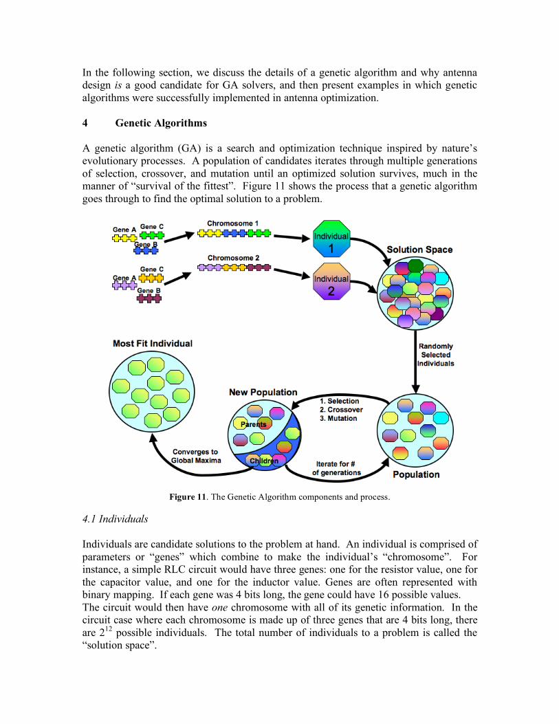
In the following section, we discuss the details of a genetic algorithm and why antenna design is a good candidate for GA solvers, and then present examples in which genetic algorithms were successfully implemented in antenna optimization. 4 Genetic Algorithms A genetic algorithm (GA) is a search and optimization technique inspired by nature’s evolutionary processes. A population of candidates iterates through multiple generations of selection, crossover, and mutation until an optimized solution survives, much in the manner of “survival of the fittest”. Figure 11 shows the process that a genetic algorithm goes through to find the optimal solution to a problem.

Figure 11. The Genetic Algorithm components and process.

4.1 Individuals Individuals are candidate solutions to the problem at hand. An individual is comprised of parameters or “genes” which combine to make the individual’s “chromosome”. For instance, a simple RLC circuit would have three genes: one for the resistor value, one for the capacitor value, and one for the inductor value. Genes are often represented with binary mapping. If each gene was 4 bits long, the gene could have 16 possible values. The circuit would then have one chromosome with all of its genetic information. In the circuit case where each chromosome is made up of three genes that are 4 bits long, there are 212 possible individuals. The total number of individuals to a problem is called the “solution space”.

4.2 Population A defined number of randomly-generated individuals establish the initial population of solutions. In order to begin the selection process of the algorithm, a fitness function must be developed that enumerates how “fit” an individual is. For instance, if we are trying to optimize an antenna’s gain and bandwidth, the fitness function would scale and combine the antenna’s gain and VSWR to determine how “fit” the antenna is. The fitness function produces one number that encompasses a combined rating of the individual’s genes. These final ratings are then used in the selection process of evolution. 4.3 Selection Based on the individual’s ratings, there are three common selection approaches to deciding which individuals continue in the process, and which are dropped. They are population decimation, proportional selection, and tournament selection. 4.3.1 Population Decimation The simplest selection scheme is population decimation in which the individuals are ranked according to their fitness ratings, and a cutoff point decimates the weakest individuals. The problem with this scheme is that traits of the discarded individuals fail to appear in subsequent generations and there is an immediate loss of diversification in the pool of individuals. 4.3.2 Proportional Selection Proportional Selection, also called the Roulette Wheel Selection, selects individuals with a probability that is proportional to their ratings. Thus, a stronger individual has a higher probability of surviving through to the next generation, but there is still a chance for a weak individual to carry through as well, a chance that did not exist in population decimation. 4.3.3 Tournament Selection Finally, Tournament Selection has been found to converge to a solution faster than Proportional Selection does, lending it the most support of the three selection schemes. In Tournament Selection, a sub-population of individuals is randomly chosen to compete on the basis of their fitness. The individuals with the highest fitness win the competition and continue to the next generation, while the other individuals are placed back into the general population and the process is repeated until a desired number of individuals have “won”. Tournament solution execution time has O(n) time complexity where Proportionate Selection has O(n^2) time complexity. 4.4 Crossover

Once the selected individuals have been established, a process of “crossover” between the individuals occurs to create new individuals. The existing individuals are called the “parents”, and the new individuals are called “children”. Crossover is applied with probability p_cross where values of .6-.8 have been found to work best in most situations (samii 15). For Parents 1 and 2 and their associated Children 1 and 2, a random number p is selected between 0 and 1. If p > p_cross, a random location in the parents’ chromosomes is selected; that portion of genetic information is copied to the non-associated child, such that both Children now have genetic information from both Parents 1 and 2. If p < p_cross, the entire chromosome of Parent 1 is copied to Child 1 and likewise for Parent 2 and Child 2. The object of crossover is to produce better combinations of genes, and thus create more fit individuals. 4.5 Mutation In addition to selection and crossover, a small percentage of individuals undergo mutation. Like crossover, mutation occurs with relation to some probability p_mutation which is normally quite low, .01-.1. With this probability, an element of an individual’s chromosome is randomly selected and changed. In binary coding, this simply means changing a “0” to a “1” or a “1” to a “0”. Mutation is another means of increasing the diversity of a population and examining parts of the solution space that may otherwise have been ignored. 4.6 Generation Once the initial population of individuals has undergone selection, crossover, and mutation, the resulting population constitutes a new “generation” and the process is repeated. The algorithm should run enough generations such that the solution converges to a global maximum. Typically, on the order of 100 generations are enough to find a solution for most problems. 4.7 Advantages and Disadvantages of Genetic Algorithms A genetic algorithm searches an entire population and does not depend on an initial set of conditions. In effect, a GA search converges to the global maximum, where other common search techniques such as Conjugate Gradient, Newton, and Simplex methods, converge to local maxima. Additionally, a GA search simply uses a cost function to assess an individual’s rating, and does not rely on local information such as derivatives, allowing it to work despite discontinuities in a solution space. Another GA advantage is its simplicity; a GA search is quite easy to understand and formulate for a designer. With these advantages, a GA search optimizer is ideal for solution spaces having:

• discontinuities • constrained parameters • large number of dimensions • many potential local maxima

The one major disadvantage to genetic algorithms is their slow convergence time. Typically, GA optimizers must evaluate every individual in a population over ~100 generations to converge to a global maxima. In antenna design, this disadvantage poses a problem because the “evaluation” of an individual requires it to be simulated; and highly-accurate EM solvers such as HFSS take quite a long time to simulate. However, Numerical Electromagnetic Code (NEC), is an electromagnetic simulator based on the Method-of-Moments technique, that offers fast, accurate, and reliable simulated results for wire structures and uses simple text input and output files. A typical simulation in NEC of less than 100 wire segments takes less than 20 seconds [11] where each version of the simple bowtie design in HFSS took to approximately 7 minutes to simulate. In GA optimization, where populations are typically around 100 individuals, and 30-50 generations are iterated, thousands of simulations must be run. Fast simulation time is necessary to make GA optimization worthwhile. 4.8 Antenna Design: Good Candidate for GA Optimization? Antenna design is a good candidate for GA optimization. Antennas have many dependent parameters that create nonlinear design problems. These parameters are either continuous, discrete, or both, and always include constraints. In this sort of solution space, finding a global maxima is key. And in electromagnetic-design problems, “convergence rate is often not nearly as important as getting a solution” [12]. Also, the standard process of antenna design relies on the manipulation of simple antennas by using traditional and intuitive techniques. However, this method of design is very limiting to the range of resulting antennas. The solution space for antennas is vast- for example, a simple RFID bowtie antenna with a double-squiggle has the following parameters:

• height length • base length • wire thickness • location of microchip • size of squiggles • type of material

Even with a limited set of parameters as shown above, the solution space is still huge. In my design process, I was limited to a local set of possible solutions, because I relied heavily on what I knew about antennas and the results of specific designs. However, GA optimizers are “non-bias” to a solution space, and thus survey the entire solution space instead of localizing on an area of interest. GA-optimizers therefore have the potential to introduce novel, non-intuitive concepts in antenna design. Below are several examples of GA-implemented antenna designs.

5 Antenna Examples When applying genetic algorithms to antenna design, there is no limit to the number of constraints the designer can set on the design. For instance, if we were applying genetic algorithms to a bowtie design, we could fixate all parameters except for base length and height length. The advantage to having a small solution space is that the GA optimizer will converge more quickly. However, the less constraints a designer places on the optimizer, the more interesting and unexpected the resulting antenna will be. The first antenna we will discuss is a good example of an antenna design with few constraints. 5.1 The Crooked Wire Genetic Antenna, Linden and Altshuler, [11] The Crooked Wire antenna is probably the most well-known GA-designed antenna due to its fascinating and non-intuitive shape. Derek Linden designed this antenna as part of his PhD thesis from MIT, with the intention of optimizing the polarization and radiation pattern. Specifically, the search was for a right-hand circularly polarized (RHCP) antenna that radiates over one hemisphere. Each wire component of the antenna was defined by its (X, Y, Z) coordinate for its start and end points. In binary GA, 5 bits were allowed for each axis coordinate, such that there were 323 possible vertices at which the wires could be connected. The antenna was composed of 7 wire segments. The cost function solely optimized the radiation pattern. Gene: 5-bits for each axis coordinate, 3 axis coordinates per point, 7 design points Chromosome/Individual: 5x3x7 = 105 bits 10010 01010 10001 11101 10101 10011 00110 10010 10111 11111 00010 10110 X1 Y1 Z1 X2 Y2 Z2 X3 Y3 Z3 X4 Y4 Z4 11000 00111 10110 00110 01011 10011 11001 10010 01101 X5 Y5 Z5 X6 Y6 Z6 X7 Y7 Z7

Cost Function: Hemispherical Coverage with RHCP—Using NEC2, computes hemispherical radiation pattern at increments of 5° in elevation (θ = -80° to +80°) and 5 percent in azimuth (φ = 0° to φ = 175°), calculates average gain for RHCP wave for elevation angles above 10°:

Score = Σfor all θ, φ[Gain(θ,φ) – Avg. Gain]2

Population: 500 individuals Crossover: 50% Mutation: Variable, <8%

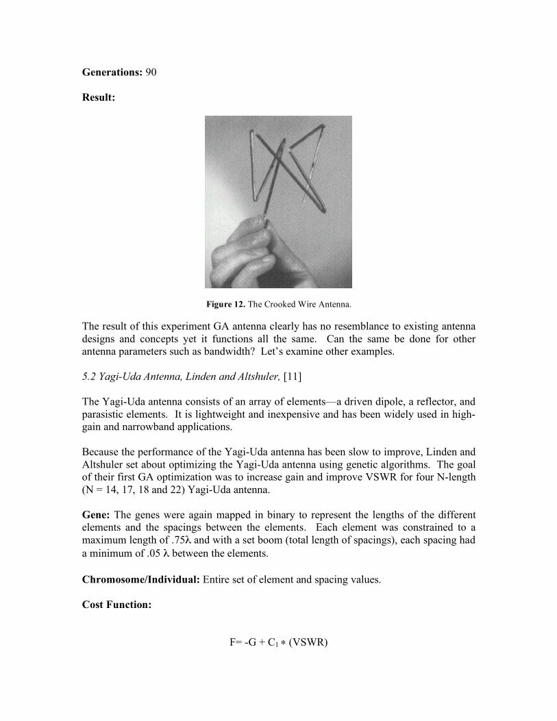
Generations: 90 Result:

Figure 12. The Crooked Wire Antenna.

The result of this experiment GA antenna clearly has no resemblance to existing antenna designs and concepts yet it functions all the same. Can the same be done for other antenna parameters such as bandwidth? Let’s examine other examples. 5.2 Yagi-Uda Antenna, Linden and Altshuler, [11] The Yagi-Uda antenna consists of an array of elements—a driven dipole, a reflector, and parasistic elements. It is lightweight and inexpensive and has been widely used in high-gain and narrowband applications. Because the performance of the Yagi-Uda antenna has been slow to improve, Linden and Altshuler set about optimizing the Yagi-Uda antenna using genetic algorithms. The goal of their first GA optimization was to increase gain and improve VSWR for four N-length (N = 14, 17, 18 and 22) Yagi-Uda antenna. Gene: The genes were again mapped in binary to represent the lengths of the different elements and the spacings between the elements. Each element was constrained to a maximum length of .75λ and with a set boom (total length of spacings), each spacing had a minimum of .05 λ between the elements. Chromosome/Individual: Entire set of element and spacing values. Cost Function:

F= -G + C1 ∗ (VSWR)

Where G is the gain, and C1 is 1 when VSWR is greater than 3.0 and .01 when VSWR is less than 3.0. The goal was to minimize F. Population: 50 Crossover: 30% Mutation: 2% Generations: N/A The GA configurations were much different from the typical Yagi antennas with the same boom length. Conventional Yagi antennas have elements whose lengths gradually decrease and spacings that gradually increase along the array. The GA Yagis however, the lengths and spacings along the array showed no pattern and appeared to be random. The GA antenna had a higher gain at the design frequency of 432 Mhz. Other GA optimizers were utilized to control gain, sidelobe level, backlobe level, VSWR, and polarization of Yagi antennas. One GA-designed antenna had low sidelobes over a specified region in space and another created a circularly polarized Yagi antenna, both design features that did not previously exist with Yagi antennas. 5.3 Broadband Patch Antenna Design, Johnson and Rahmat-Samii, [13]

The next example is a simple patch antenna that was optimized to produce a wider operational bandwidth than classical designs. Specifically, the goal was to produce a patch antenna with a 2:1 VSWR over 20% bandwidth centered at 3GHz. A 5.0 x 5.0 cm patch was suspended .5cm above a groundplane as shown in Figure 13. The GA optimized the patch by removing square metal subsections from the patch region.

Figure 13. The 5cm 5cm patch before GA-optimization.

Gene: 1-bit string representing the presence or absence of a subsection of metal in the patch Chromosome/Individual: λ/2 square patch, fed by simple wire feed Cost functions: Minimize S11 magnitude at three frequencies, 2.7 Ghz, 3 Ghz, and 3.3 Ghz. The s-parameter S11 is yet another metric to measure the reflection of energy

between two media, like Γ and VSWR. A value of S11 = -10 dB corresponds to a VSWR value of 2. Therefore, S11< -10dB signifies the antenna’s impedance bandwidth.

Fitness = min (S11n)

∀n

Population: 100 Individuals Crossover: 70% Mutation: 2% Generations: 100 Result:

Figure 14. The GA-optimized patch and its S-paramter. From Figure 14, we see that before optimization, the patch antenna had a bandwidth of approximately 6%. After GA optimization, this BW increased to the desired 20.6%. 5.4 Broadband Patch Antenna Design #2, Choo et. al., [14] In this research, Choo et. Al. use a similar approach to designing a broadband patch antenna as the Johnson patch antenna described above. Again, they began with a metallic patch, in which sub-patches were represented by either ones (metal) or zeros (no metal). The goal was to broaden the bandwidth of a microstrip antenna around a center frequency of 2 Ghz by changing the patch shape. The implemented cost function was defined as the average S11 values that exceed -10dB within the frequency range of interest.

Figure 15. The GA-optimized patch and its S-parameter.

The bandwidth of this design is found to be ~8 % by simulation and measurement where a regular square microstrip antenna (36 x 36 mm) has a bandwidth of only 1.98%. This four-fold increase in bandwidth is a result of creating an unusual ragged-shaped patch antenna that makes no intuitive sense.

5.5 Dual-Band Patch Antenna Design, Villegas, et al., [15] The goal of this paper was to design a dual-band patch antenna for wireless communications operating at 1.9 Ghz and 2.4 Ghz. The hybrid fitness function combines the VSWR at the desire frequencies as well as the cross-polarized far field (low desired). Gene: Like other GA patch antennas, 1-bit string representing the presence or absence of a subsection of metal in the patch. Chromosome/Individual: 2D rectangular array of 46 binary metallic elements. Population: 260 Crossover: 70% Mutation: 5% Generations: 200 Results:

Figure 16.The resulting GA-optimized patch antenna design for dual operation at 1.9Ghz and 2.4 Ghz.

The resulting design has 5.3% and 7% operating bandwidths at 1.9 Ghz and 2.4 Ghz. 5.6 Using GAs To Compare the Bandwidth Performance of Bowtie and Reverse Bowtie Antenna Designs, Kerkhoff, et al., [16] This study not only used genetic algorithms to optimize specific antenna designs, but compared the GA-optimized designs to determine which design has better bandwidth performance. The two designs are the bowtie antenna and the reverse bowtie antenna, both over an infinite ground plane as shown in Figure BLAH. Gene: The antenna height H and the flare angle α were the variable genes in this experiment. The reverse bowtie had an additional parameter, the feed height hf which is the distance of the feed point above the groundplane. Chromosome/Individual: Bowtie or reverse bowtie antenna with specified height H, flare angle α, and feed height hf in the case of the reverse bowtie. Population: For each antenna type, population size was 60. Crossover: 50% Mutation: 2-4% Generations: N/A/ Results:

(a) (b)

Figure 17. The results of the (a) Bowtie Antenna and the (b) Reverse Bowtie Antenna.

The results showed that the RBT could achieve 80% fractional bandwidth with a significantly smaller size than the regular BT. Fractional bandwidth means that 20% fractional bandwidth around 1 Ghz would be 900Mhz-111Mhz. The GA-optimized antennas were also built and physically tested, of which the measured results matched the simulated results:

Figure 18. Measured and simulated results of 30% and 70% bandwidth reverse bowtie design. The implications of this paper are more than that the RBT has a better broadband performance than the regular bowtie design. The paper also demonstrates that genetic algorithms are an effective way of evaluating antennas, and specifically the bandwidth of antennas.

Conlusions Genetic algorithms have clearly been effective in many aspects of antenna design. Will they do the same for UHF RFID antenna design? All the signs point toward yes, but the only way to really find out is to actually create a GA-optimized tag antenna. To recap, GA optimizers are good for solutions spaces having:

• discontinuities • constrained parameters • large number of dimensions • many potential local maxima

RFID tag antennas have many constraints including:

• size • cost • planar configuration • polarization

Figure 19. Existing passive UHF RFID tags manufactured by Alien Technology and Avery Dennison. The antenna configurations shown in Figure 19 seem creative and interesting but they were all developed using traditional techniques such as folded dipoles, squiggles, and fanning. Their designs were all limited to the scope of the designer’s knowledge and intuition. The solution space of antennas far exceeds a designer’s notions. In the case of a simple bowtie antenna, we showed that many dimensions can be altered including:

• height length

• base length • wire thickness • location of microchip • size of squiggles • type of material

Because of the initial conditions and limitations that antenna designers are constrained by, the resulting antenna designs shown above might be the results of local maxima, rather than global maxima of the solution space. For the design of new bowtie designs, I propose two GA-optimized antennas. The first will be a GA-optimized version of my bowtie design from Section 3. The area of the antenna will be limited to the size of Avery Dennison’s 5.5 in x .98 in bowtie design. The “genes” in the optimization will be the length of the triangle height, the length of the triangle base, and the squiggle length. The fitness function will measure and scale an individual’s gain and VSWR, similar to the fitness function that Linden and Altshuler used for their GA-optimized Yagi antenna:

F= -G + C1 ∗ (VSWR) Since this design is made up of “wires”, it can easily be simulation using Numerical Electromagnetic Code (NEC). The second design I am interested in looking at is optimizing a full-metal bowtie by implementing the patch chromosome method that we saw in antenna examples 3, 4, and 5—where a “gene” is a subpatch of metal and can have a value of “1” to represent the presence of metal or “0” to represent its absence. For this design, I would set the dimensions to 5.5 in x .98 in. The fitness function would measure the gain, the VSWR, and it would also include a component about how much metal is used. Cost is a huge issue in passive RFID and we want to make sure that we were making affordable tags- otherwise, RFID is pointless. The fitness function would look something like this:

F = -G + C1 ∗ (VSWR) + M where M represent the total amount of copper used. From the examples we saw earlier, I expect that this GA-optimization will lead to some very interesting and non-intuitive designs. In general, passive UHF RFID tag antenna design has proven to be very challenging. Existing tag antennas are not nearly effective enough- or small enough- or cheap enough. Using genetic algorithms to design tag antennas introduces an opportunity to investigate untapped territory and potentially discover designs that can satisfy RFID requirements. The simplicity of genetic algorithms and the efficiency of fast simulators such as NEC make the application of GA-optimized RFID tag antennas very realizable.

References [1] S. Rutner, et. al, “A practical look at RFID,” Supply Chain Management Review, January/February 2004. [2] M. Roberti, “EPCglobal ratifies Gen 2 Standard,” RFIDJournal, Dec. 2004. [3] A. Delichatsios, D.W. Engels, “The Albano passive UHF RFID tag antenna,” Waveform Diversity Conference, Jan. 2006. [4] Ansoft Corporation, http://www.ansoft.com/products/hf/hfss/. HFSS: 3D Electromagnetic-Field Simulation for High-Performance Electronic Design, 2006. [5] J. A. Kong, Electromagnetic Wave Theory. Cambridge, MA: EMW Publishing, 2000. [6] A. Stace, “Use of Genetic Algorithms in Electromagnetics,” Bachelors thesis, University of Queensland, Oct. 1997. [7] A. Marczyk, “Genetic algorithms and evolutionary computation,” The Talk.Origins Archive, 2004. http://www.talkorigins.org/faqs/genalg/genalg.html. [8] Y. Rahmat-Samii, E. Michielssen, Electromagnetic Optimization by Genetic Algorithms. New York: John Wiley and Sons, Inc., 1999. [9] R.J. Marhefka, D.D. Kraus, Antennas For All Applications, 3rd ed. New York: McGraw-Hill, 2002. [10] J.A. Kuecken, Antennas and Transmission Lines. USA: MFJ Enterprises, Inc., 1996. [11] D. S. Linden, “Automated design and optimization of wire antennas using genetic algorithms,” PhD thesis, MIT, Cambridge, MA, Sept. 1997. [12] J.M. Johnson and Y. Rahmat-Samii, “Genetic algorithms in engineering electromagnetics,” IEEE Antennas Propagat. Mag., vol. 39, pp. 7-25, Aug. 1997. [13] J. M. Johnson, Y. Rahmat-Samii, “Genetic algorithms and method of moments (GA/MoM) for the design of integrated antennas,” IEEE Trans. Antennas Propagat., vol. 47, pp 1606-1614, Oct 1999. [14] H. Choo, A. Hutani, L.C. Trintinalia, and H. Ling, “Shape optimization of broadband microstrip antennas using genetic algorithm,”Electronic Letters, vol. 36, no. 25, pp. 2057-2058, Dec. 2000.

[15] F. Villegas, T. Cwik, Y. Rahmat-Samii, M. Manteghi, “A parallel electromagnetic genetic-algorithm optimization (EGO) application for patch antenna design,” IEEE Trans. Antennas Propagat., vol. 52, no. 9, September 2004. [16] A. Kerkhoff, R. Rogers, and H. Ling, “The use of the genetic algorithm approach in the design of ultra-wideband antennas,” Proc. IEEE Radio and Wireless Conference, Aug. 2001, pp 93-96.