funktionen-katalog - mathe online · funktionen-katalog i. geraden ii. ganzrationale funktion:...
TRANSCRIPT
Funktionskatalog
© [email protected] / www.rudolf-web.de 1
Funktionen-Katalog I. Geraden II. Ganzrationale Funktion: Parabeln 2-ten Grades | 3-ten Grades | Parabeln höheren Grades III. Gebrochenrationale Funktionen: Asymptoten, Polstellen ... IV. Exponentialfunktionen V. Trigonometrische Funktionen: Sinus, Kosinus, Tangens, Allgemeine Sinusfunktion VI. Überblick über die wichtigsten Funktionen
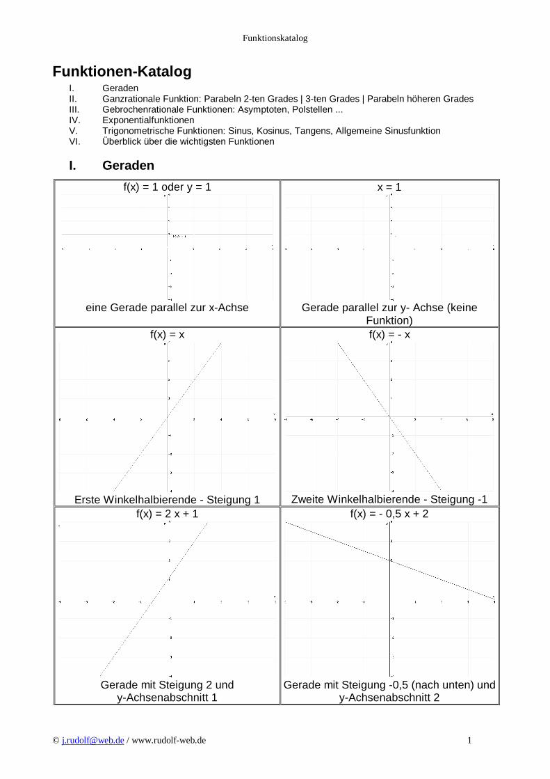
I. Geraden
f(x) = 1 oder y = 1
eine Gerade parallel zur x-Achse
x = 1
Gerade parallel zur y- Achse (keine
Funktion) f(x) = x
Erste Winkelhalbierende - Steigung 1
f(x) = - x
Zweite Winkelhalbierende - Steigung -1
f(x) = 2 x + 1
Gerade mit Steigung 2 und
y-Achsenabschnitt 1
f(x) = - 0,5 x + 2
Gerade mit Steigung -0,5 (nach unten) und
y-Achsenabschnitt 2
Funktionskatalog
© [email protected] / www.rudolf-web.de 2
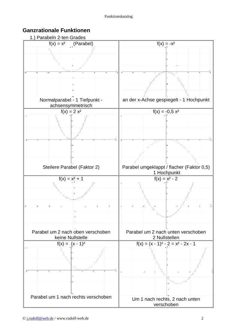
Ganzrationale Funktionen 1.) Parabeln 2-ten Grades
f(x) = x² (Parabel)
Normalparabel - 1 Tiefpunkt -
achsensymmetrisch
f(x) = -x²
an der x-Achse gespiegelt - 1 Hochpunkt
f(x) = 2 x²
Steilere Parabel (Faktor 2)
f(x) = -0,5 x²
Parabel umgeklappt / flacher (Faktor 0,5)
1 Hochpunkt f(x) = x² + 1
Parabel um 2 nach oben verschoben
keine Nullstelle
f(x) = x² - 2
Parabel um 2 nach unten verschoben
2 Nullstellen f(x) = (x - 1)²
Parabel um 1 nach rechts verschoben
f(x) = (x - 1)² - 2 = x² - 2x - 1
Um 1 nach rechts, 2 nach unten
verschoben
Funktionskatalog
© [email protected] / www.rudolf-web.de 3
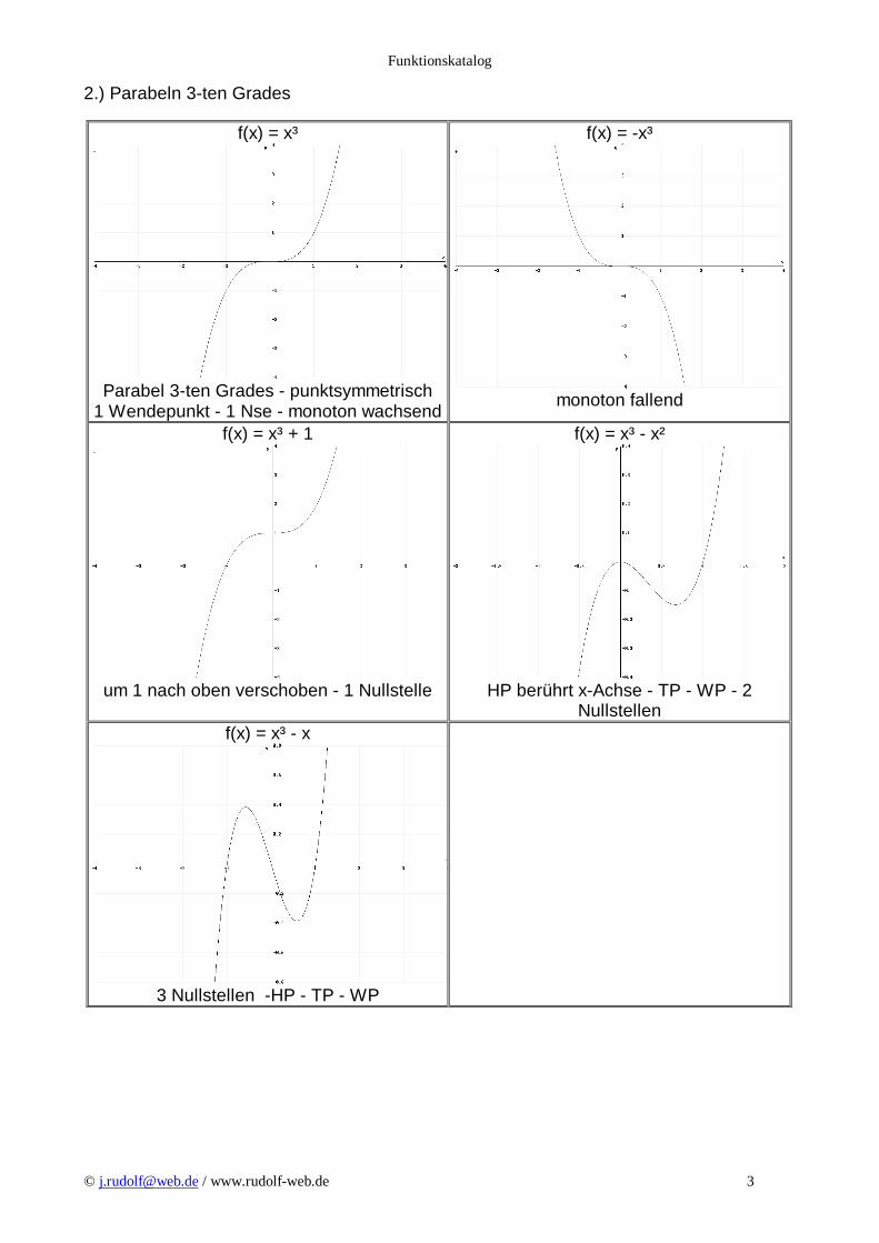
2.) Parabeln 3-ten Grades
f(x) = x³
Parabel 3-ten Grades - punktsymmetrisch
1 Wendepunkt - 1 Nse - monoton wachsend
f(x) = -x³
monoton fallend
f(x) = x³ + 1
um 1 nach oben verschoben - 1 Nullstelle
f(x) = x³ - x²
HP berührt x-Achse - TP - WP - 2
Nullstellen f(x) = x³ - x
3 Nullstellen -HP - TP - WP
Funktionskatalog
© [email protected] / www.rudolf-web.de 4
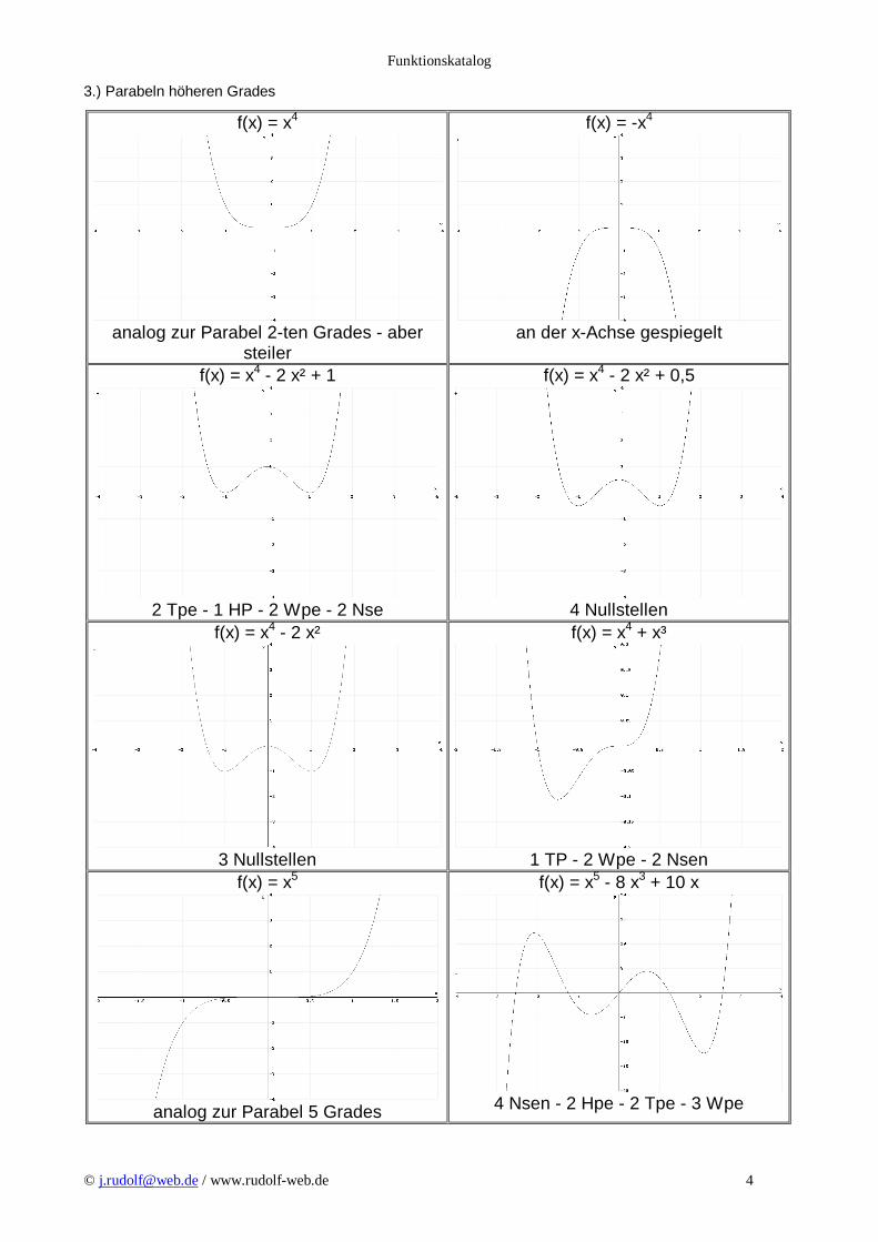
3.) Parabeln höheren Grades
f(x) = x4
analog zur Parabel 2-ten Grades - aber
steiler
f(x) = -x4
an der x-Achse gespiegelt
f(x) = x4 - 2 x² + 1
2 Tpe - 1 HP - 2 Wpe - 2 Nse
f(x) = x4 - 2 x² + 0,5
4 Nullstellen
f(x) = x4 - 2 x²
3 Nullstellen
f(x) = x4 + x³
1 TP - 2 Wpe - 2 Nsen
f(x) = x5
analog zur Parabel 5 Grades
f(x) = x5 - 8 x3 + 10 x
4 Nsen - 2 Hpe - 2 Tpe - 3 Wpe
Funktionskatalog
© [email protected] / www.rudolf-web.de 5
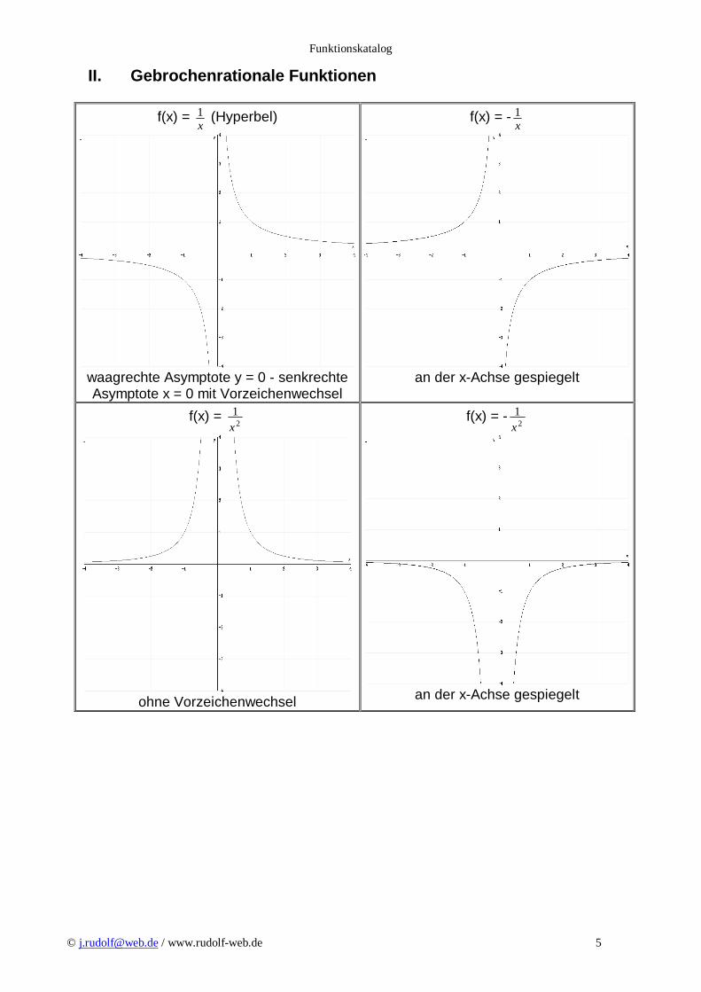
II. Gebrochenrationale Funktionen
f(x) = x1 (Hyperbel)
waagrechte Asymptote y = 0 - senkrechte Asymptote x = 0 mit Vorzeichenwechsel
f(x) = -x1
an der x-Achse gespiegelt
f(x) = 2
1x
ohne Vorzeichenwechsel
f(x) = -2
1x
an der x-Achse gespiegelt
Funktionskatalog
© [email protected] / www.rudolf-web.de 6
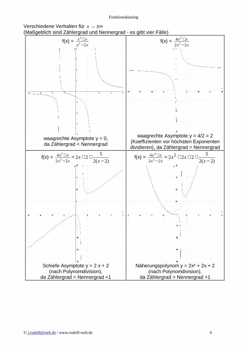
Verschiedene Verhalten für ±∞→x (Maßgeblich sind Zählergrad und Nennergrad - es gibt vier Fälle)
f(x) = xxxx
23
2
−+
waagrechte Asymptote y = 0, da Zählergrad < Nennergrad
f(x) = xx
xx22
42
2
−+
waagrechte Asymptote y = 4/2 = 2
(Koeffizienten vor höchsten Exponenten dividieren), da Zählergrad = Nennergrad
f(x) = )2(2
522
224
2
3
−++=
−+
xx
xx
xx
Schiefe Asymptote y = 2 x + 2
(nach Polynomdivision), da Zählergrad = Nennergrad +1
f(x) = )2(2
5222 2
224
2
4
−+++=
−+
xxx
xx
xx
Näherungspolynom y = 2x² + 2x + 2
(nach Polynomdivision), da Zählergrad > Nennergrad +1
Funktionskatalog
© [email protected] / www.rudolf-web.de 7
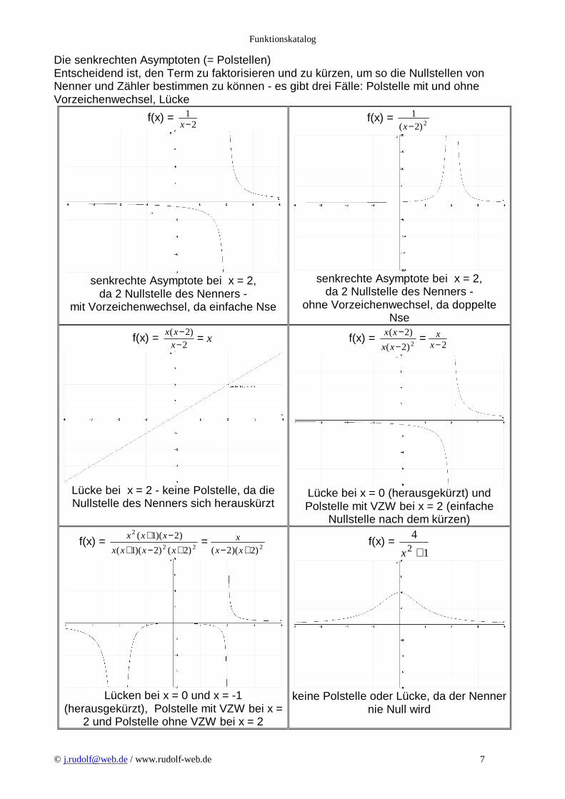
Die senkrechten Asymptoten (= Polstellen) Entscheidend ist, den Term zu faktorisieren und zu kürzen, um so die Nullstellen von Nenner und Zähler bestimmen zu können - es gibt drei Fälle: Polstelle mit und ohne Vorzeichenwechsel, Lücke
f(x) = 2
1−x
senkrechte Asymptote bei x = 2,
da 2 Nullstelle des Nenners - mit Vorzeichenwechsel, da einfache Nse
f(x) = 2)2(
1−x
senkrechte Asymptote bei x = 2,
da 2 Nullstelle des Nenners - ohne Vorzeichenwechsel, da doppelte
Nse
f(x) = xxxx =−
−2
)2(
Lücke bei x = 2 - keine Polstelle, da die Nullstelle des Nenners sich herauskürzt
f(x) = 2)2(
)2(2 −−
− =x
xxx
xx
Lücke bei x = 0 (herausgekürzt) und Polstelle mit VZW bei x = 2 (einfache
Nullstelle nach dem kürzen)
f(x) = 222
2
)2)(2()2()2)(1(
)2)(1(
+−+−+−+ =
xxx
xxxx
xxx
Lücken bei x = 0 und x = -1
(herausgekürzt), Polstelle mit VZW bei x = 2 und Polstelle ohne VZW bei x = 2
f(x) = 1
42 +x
keine Polstelle oder Lücke, da der Nenner
nie Null wird
Funktionskatalog
© [email protected] / www.rudolf-web.de 8
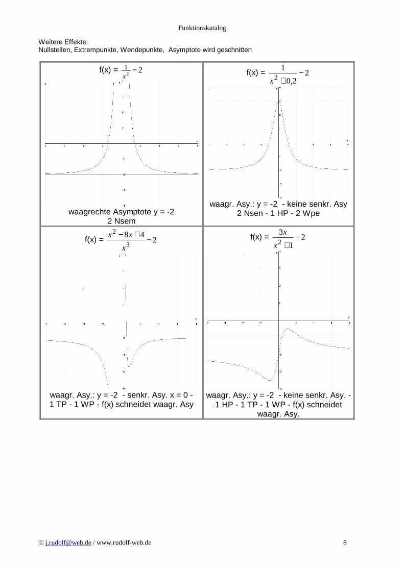
Weitere Effekte: Nullstellen, Extrempunkte, Wendepunkte, Asymptote wird geschnitten
f(x) = 22
1 −x
waagrechte Asymptote y = -2
2 Nsem
f(x) = 22,0
12
−+x
waagr. Asy.: y = -2 - keine senkr. Asy
2 Nsen - 1 HP - 2 Wpe
f(x) = 248
3
2−+−
x
xx
waagr. Asy.: y = -2 - senkr. Asy. x = 0 - 1 TP - 1 WP - f(x) schneidet waagr. Asy
f(x) = 21
32
−+x
x
waagr. Asy.: y = -2 - keine senkr. Asy. -
1 HP - 1 TP - 1 WP - f(x) schneidet waagr. Asy.
Funktionskatalog
© [email protected] / www.rudolf-web.de 9
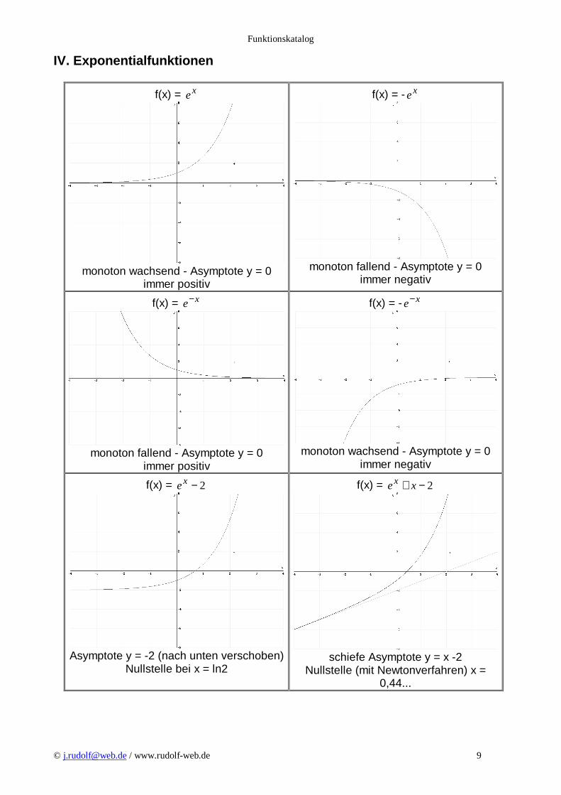
IV. Expon entialfunktionen
f(x) = xe
monoton wachsend - Asymptote y = 0
immer positiv
f(x) = - xe
monoton fallend - Asymptote y = 0
immer negativ
f(x) = xe−
monoton fallend - Asymptote y = 0
immer positiv
f(x) = - xe−
monoton wachsend - Asymptote y = 0
immer negativ
f(x) = 2−xe
Asymptote y = -2 (nach unten verschoben)
Nullstelle bei x = ln2
f(x) = 2−+ xe x
schiefe Asymptote y = x -2
Nullstelle (mit Newtonverfahren) x = 0,44...
Funktionskatalog
© [email protected] / www.rudolf-web.de 10
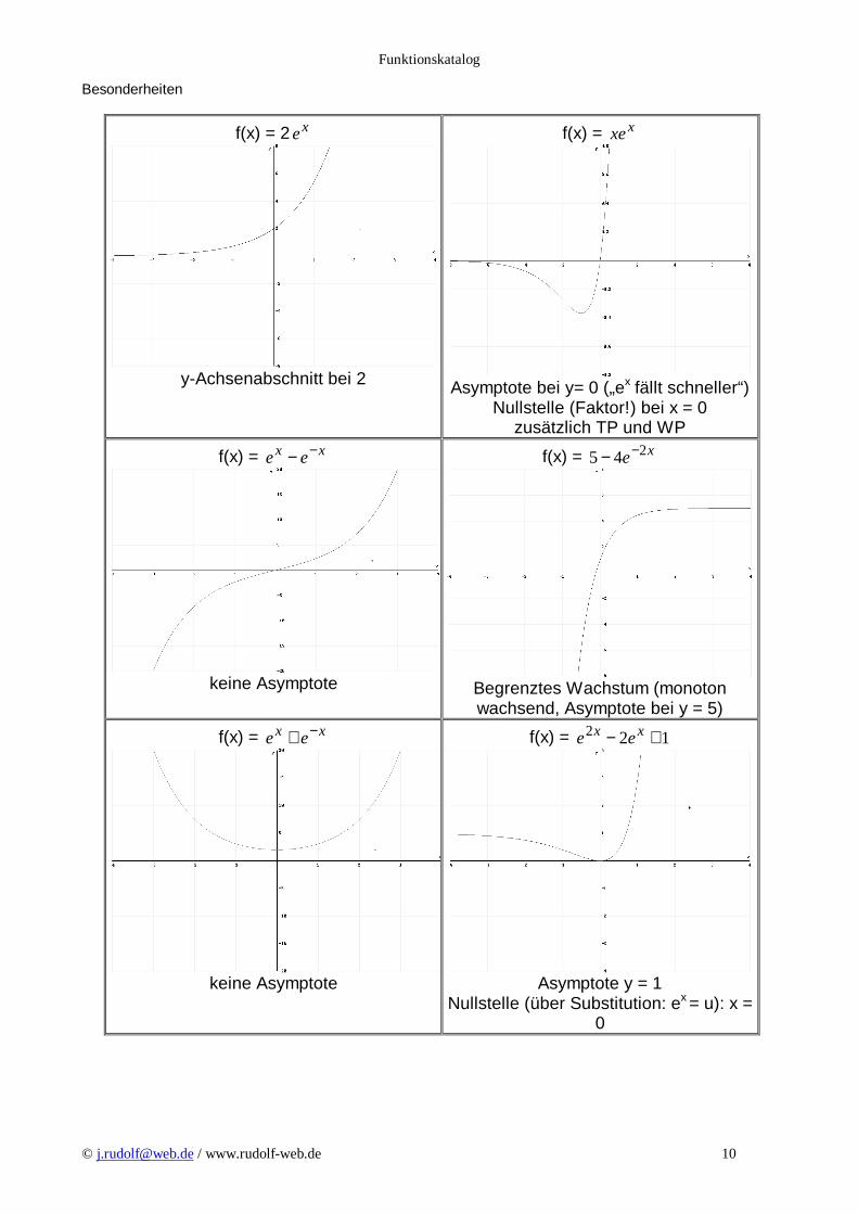
Besonderheiten
f(x) = 2 xe
y-Achsenabschnitt bei 2
f(x) = xxe
Asymptote bei y= 0 („ex fällt schneller“)
Nullstelle (Faktor!) bei x = 0 zusätzlich TP und WP
f(x) = xx ee −−
keine Asymptote
f(x) = xe 245 −−
Begrenztes Wachstum (monoton wachsend, Asymptote bei y = 5)
f(x) = xx ee −+
keine Asymptote
f(x) = 122 +− xx ee
Asymptote y = 1
Nullstelle (über Substitution: ex = u): x = 0
Funktionskatalog
© [email protected] / www.rudolf-web.de 11
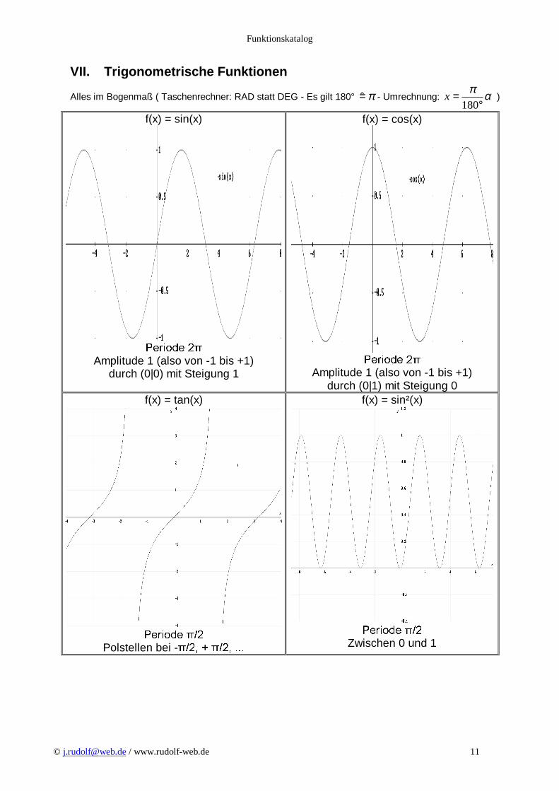
VII. Trigono metrische Funktionen
Alles im Bogenmaß ( Taschenrechner: RAD statt DEG - Es gilt 180° π=̂ - Umrechnung: απ°
=180
x )
f(x) = sin(x)
� � � � � � � � �
Amplitude 1 (also von -1 bis +1) durch (0|0) mit Steigung 1
f(x) = cos(x)
� � � � �
Amplitude 1 (also von -1 bis +1) durch (0|1) mit Steigung 0
f(x) = tan(x)
� � � � � �
Polstellen bei - � � � � � � � � � � � �
f(x) = sin²(x)
� � � � � � ! � � Zwischen 0 und 1
Funktionskatalog
© [email protected] / www.rudolf-web.de 12
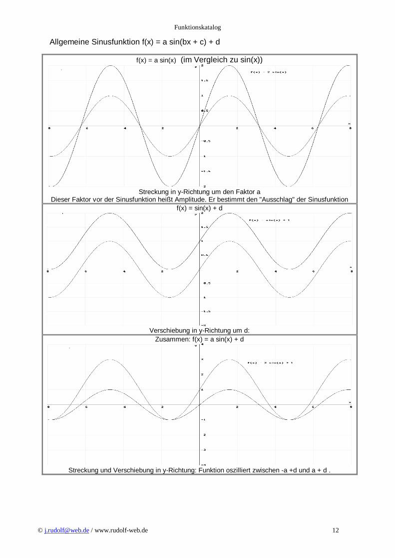
Allgemeine Sinusfunktion f(x) = a sin(bx + c) + d
f(x) = a sin(x) (im Vergleich zu sin(x))
Streckung in y-Richtung um den Faktor a
Dieser Faktor vor der Sinusfunktion heißt Amplitude. Er bestimmt den "Ausschlag" der Sinusfunktion f(x) = sin(x) + d
Verschiebung in y-Richtung um d:
Zusammen: f(x) = a sin(x) + d
Streckung und Verschiebung in y-Richtung: Funktion oszilliert zwischen -a +d und a + d .
Funktionskatalog
© [email protected] / www.rudolf-web.de 13
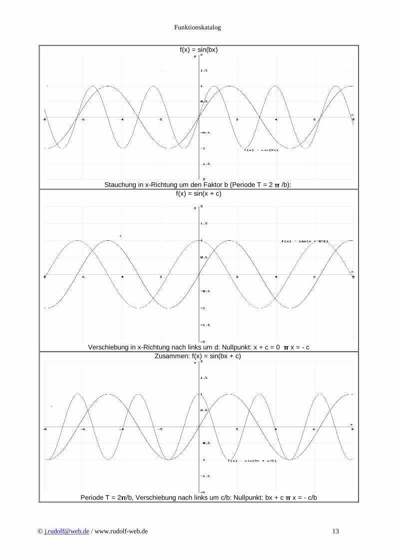
f(x) = sin(bx)
Stauchung in x-Richtung um den Faktor b (Periode T = 2 " /b):
f(x) = sin(x + c)
Verschiebung in x-Richtung nach links um d: Nullpunkt: x + c = 0 " x = - c
Zusammen: f(x) = sin(bx + c)
Periode T = 2" /b, Verschiebung nach links um c/b: Nullpunkt: bx + c " x = - c/b
Funktionskatalog
© [email protected] / www.rudolf-web.de 14
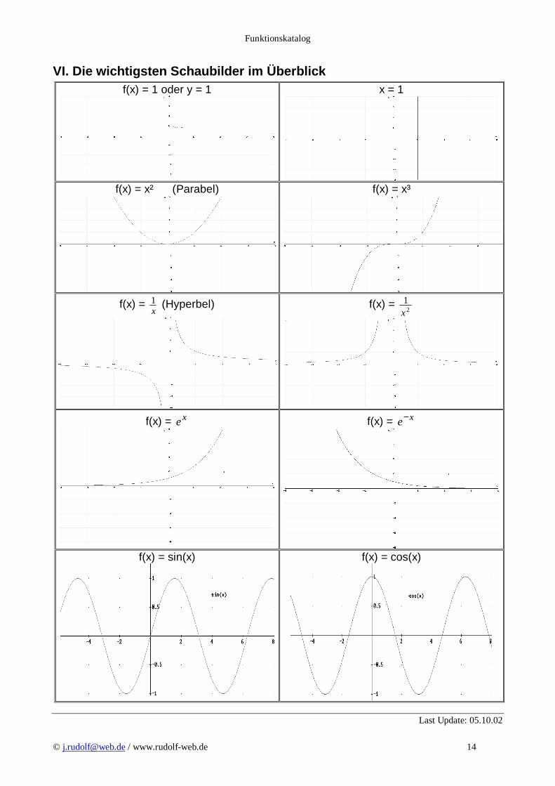
VI. Die wichtigsten Schaubilder im Überblick f(x) = 1 oder y = 1
x = 1
f(x) = x² (Parabel)
f(x) = x³
f(x) = x1 (Hyperbel)
f(x) = 2
1x
f(x) = xe
f(x) = xe−
f(x) = sin(x)
f(x) = cos(x)
Last Update: 05.10.02