full-stack optimization for accelerating cnnswith fpga ... · full-stack optimization for...
TRANSCRIPT
Full-stack Optimization for Accelerating CNNswith FPGA Validation
Bradley McDanel∗Harvard University
Sai Qian Zhang∗Harvard University
H.T. KungHarvard [email protected]
Xin DongHarvard University
ABSTRACTWe present a full-stack optimization framework for accelerating in-ference of CNNs (Convolutional Neural Networks) and validate theapproach with field-programmable gate arrays (FPGA) implementa-tions. By jointly optimizing CNN models, computing architectures,and hardware implementations, our full-stack approach achievesunprecedented performance in the trade-off space characterizedby inference latency, energy efficiency, hardware utilization andinference accuracy. As a validation vehicle, we have implementeda 170MHz FPGA inference chip achieving 2.28ms latency for theImageNet benchmark. The achieved latency is among the lowest re-ported in the literature while achieving comparable accuracy. How-ever, our chip shines in that it has 9x higher energy efficiency com-pared to other implementations achieving comparable latency. Ahighlight of our full-stack approachwhich attributes to the achievedhigh energy efficiency is an efficient Selector-Accumulator (SAC)architecture for implementing the multiplier-accumulator (MAC)operation present in any digital CNN hardware. For instance, com-pared to a FPGA implementation for a traditional 8-bit MAC, SACsubstantially reduces required hardware resources (4.85x fewerLook-up Tables) and power consumption (2.48x).
Final version will appear in InternationalConference on Supercomputing (ICS) 2019.
1 INTRODUCTIONDue to the widespread success of Convolutional Neural Networks(CNNs) across a variety of domains, there have been extraordinaryresearch and development efforts placed on improving inference la-tency, energy efficiency, and accuracy of these networks. Generally,these research efforts can be viewed from two distinct perspec-tives: (1) machine learning practitioners who focus on reducingthe complexity of CNNs through more efficient convolution oper-ations [44], weight and activation quantization [22], and weightpruning [14] and (2) hardware architecture experts who design andbuild CNN accelerators with minimal power consumption and I/Ocost [11, 23, 42, 46].
However, approaching the problem from only one of these twoviewpoints can lead to suboptimal solutions. For instance, as dis-cussed in Section 2.3, many low-precision weight quantizationmethods omit certain significant cost factors in an end-to-end im-plementation such as using full-precision weights and data forthe first and last layers [4, 48] or full-precision batch normaliza-tion [21] as in [36]. On the other side, most CNN accelerators are
*Equal Contribution.
Streamlined CNN Architecture and Full-Stack Model Training
Training Data
{‘rose’,…, ‘dog’}
...
1x1 conv, 64, 2shift+1x1 conv, 128, 1
StreamlinedCNN Architectureshift+1x1 conv, 512, 1
Quantization-aware TrainingFor Power of Two Weights
output
linear quant
input weights
log quant
convolution
folded batchnorm
Configuration and Instructions of CNN
Section 3
Trained CNN Model
Section 4
0 0 2-2 0
2-30 0 0
00 0 2-1
0 21 0 0
-
Packed FormatCNN Layer
Generate Instructions
01010110
00010101
01100111
01010110
Coding Sparse CNN Layers
Hardware Design for CNN Inference
Section 5
Target FPGA
Systolic Array Architecture
Load Weight: layer 1, tile 1, 64x48Matrix Multiply: input data, 48x56x56Load Weight: layer 2, tile 1, 128x64Matrix Multiply: layer 1 data, 64x56x56
Load Weight: layer 18, tile 1, 128x512
...
Quantizer
Data Buffer
ParameterBuffer
Host
power of two shifts via shared
register chain
SystolicCells
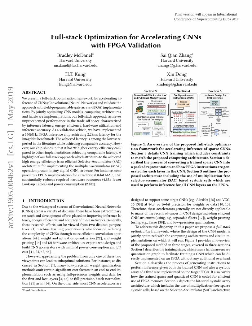
Figure 1: An overview of the proposed full-stack optimiza-tion framework for accelerating inference of sparse CNNs.Section 3 details CNN training which includes constraintsto match the proposed computing architecture. Section 4 de-scribed the process of converting a trained sparse CNN intoa packed representation and how FPGA instructions are gen-erated for each layer in the CNN. Section 5 outlines the pro-posed architecture including the use of multiplication-freeselector-accumulator (SAC) based systolic cells which areused to perform inference for all CNN layers on the FPGA.
designed to support some target CNNs (e.g., AlexNet [26] and VGG-16 [38]) at 8-bit or 16-bit precision for weights or data [10, 13].Therefore, these accelerators generally are not directly applicableto many of the recent advances in CNN design including efficientCNN structures (using, e.g., separable filters [17]), weight pruning(using, e.g., Lasso [39]), and low-precision quantization.
To address this disparity, in this paper we propose a full-stackoptimization framework, where the design of the CNN model isjointly optimized with the computing architectures and circuit im-plementations on which it will run. Figure 1 provides an overviewof the proposed method in three stages, covered in three sections.Section 3 describes the training stage, which uses a hardware-awarequantization graph to facilitate training a CNN which can be di-rectly implemented on an FPGA without any additional overhead.
Section 4 describes the process of generating instructions toperform inference given both the trained CNN and also a systolicarray of a fixed size implemented on the target FPGA. It also covershow the trained sparse and quantized CNN is coded for efficientuse of FPGA memory. Section 5 depicts the bit-serial systolic arrayarchitecture which includes the use of multiplication-free sparsesystolic cells, based on the Selector-Accumulator (SAC) architecture
arX
iv:1
905.
0046
2v1
[cs
.LG
] 1
May
201
9
Layer LWeight Matrix
128
128
Layer L+1Weight Matrix
256
128
Layer L
Layer L+1
Tile 1
Tile 1
Tile 2
SystolicArray
Layer L, Tile 1Layer L-1Output
Layer LOutput
Layer LOutput
Layer L+1, Tile 1
Layer L+1, Tile 2
All layers processed
on-chip
Layer L Output is
Layer L+1 Input
Load Weights
Matrix Multiply
128
128
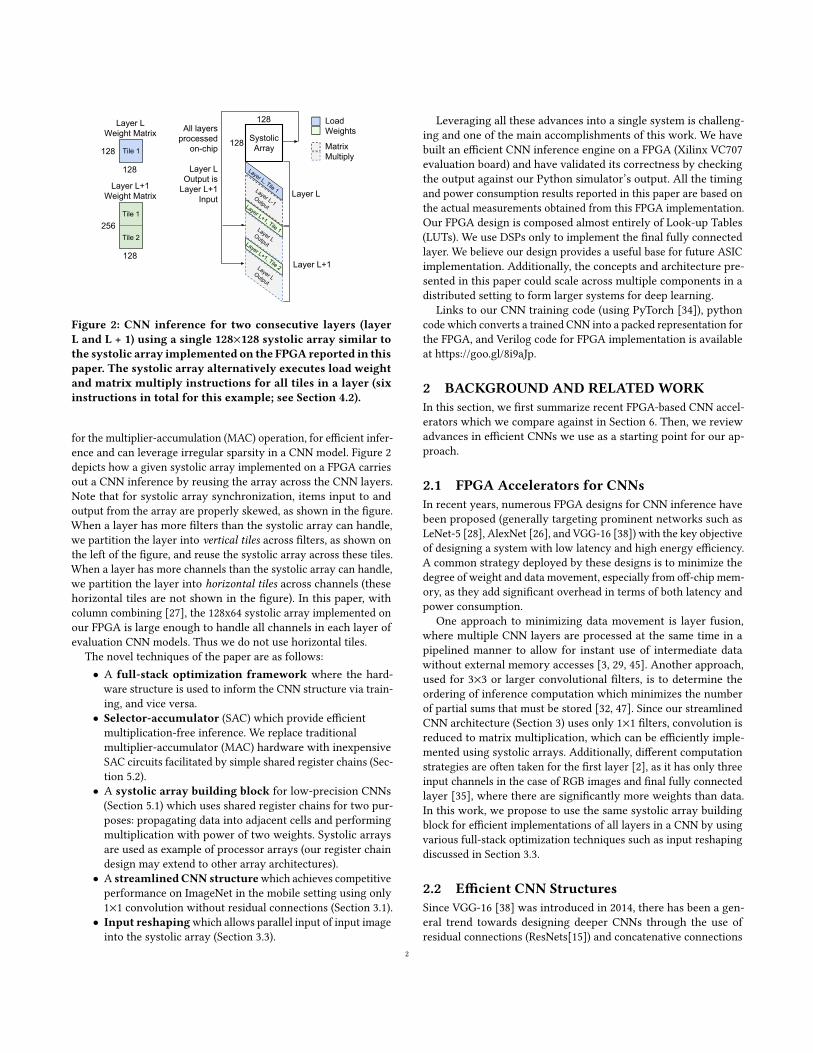
Figure 2: CNN inference for two consecutive layers (layerL and L + 1) using a single 128×128 systolic array similar tothe systolic array implemented on the FPGA reported in thispaper. The systolic array alternatively executes load weightand matrix multiply instructions for all tiles in a layer (sixinstructions in total for this example; see Section 4.2).
for the multiplier-accumulation (MAC) operation, for efficient infer-ence and can leverage irregular sparsity in a CNN model. Figure 2depicts how a given systolic array implemented on a FPGA carriesout a CNN inference by reusing the array across the CNN layers.Note that for systolic array synchronization, items input to andoutput from the array are properly skewed, as shown in the figure.When a layer has more filters than the systolic array can handle,we partition the layer into vertical tiles across filters, as shown onthe left of the figure, and reuse the systolic array across these tiles.When a layer has more channels than the systolic array can handle,we partition the layer into horizontal tiles across channels (thesehorizontal tiles are not shown in the figure). In this paper, withcolumn combining [27], the 128x64 systolic array implemented onour FPGA is large enough to handle all channels in each layer ofevaluation CNN models. Thus we do not use horizontal tiles.
The novel techniques of the paper are as follows:• A full-stack optimization framework where the hard-ware structure is used to inform the CNN structure via train-ing, and vice versa.
• Selector-accumulator (SAC) which provide efficientmultiplication-free inference. We replace traditionalmultiplier-accumulator (MAC) hardware with inexpensiveSAC circuits facilitated by simple shared register chains (Sec-tion 5.2).
• A systolic array building block for low-precision CNNs(Section 5.1) which uses shared register chains for two pur-poses: propagating data into adjacent cells and performingmultiplication with power of two weights. Systolic arraysare used as example of processor arrays (our register chaindesign may extend to other array architectures).
• A streamlinedCNN structurewhich achieves competitiveperformance on ImageNet in the mobile setting using only1×1 convolution without residual connections (Section 3.1).
• Input reshapingwhich allows parallel input of input imageinto the systolic array (Section 3.3).
Leveraging all these advances into a single system is challeng-ing and one of the main accomplishments of this work. We havebuilt an efficient CNN inference engine on a FPGA (Xilinx VC707evaluation board) and have validated its correctness by checkingthe output against our Python simulator’s output. All the timingand power consumption results reported in this paper are based onthe actual measurements obtained from this FPGA implementation.Our FPGA design is composed almost entirely of Look-up Tables(LUTs). We use DSPs only to implement the final fully connectedlayer. We believe our design provides a useful base for future ASICimplementation. Additionally, the concepts and architecture pre-sented in this paper could scale across multiple components in adistributed setting to form larger systems for deep learning.
Links to our CNN training code (using PyTorch [34]), pythoncode which converts a trained CNN into a packed representation forthe FPGA, and Verilog code for FPGA implementation is availableat https://goo.gl/8i9aJp.
2 BACKGROUND AND RELATEDWORKIn this section, we first summarize recent FPGA-based CNN accel-erators which we compare against in Section 6. Then, we reviewadvances in efficient CNNs we use as a starting point for our ap-proach.
2.1 FPGA Accelerators for CNNsIn recent years, numerous FPGA designs for CNN inference havebeen proposed (generally targeting prominent networks such asLeNet-5 [28], AlexNet [26], and VGG-16 [38]) with the key objectiveof designing a system with low latency and high energy efficiency.A common strategy deployed by these designs is to minimize thedegree of weight and data movement, especially from off-chip mem-ory, as they add significant overhead in terms of both latency andpower consumption.
One approach to minimizing data movement is layer fusion,where multiple CNN layers are processed at the same time in apipelined manner to allow for instant use of intermediate datawithout external memory accesses [3, 29, 45]. Another approach,used for 3×3 or larger convolutional filters, is to determine theordering of inference computation which minimizes the numberof partial sums that must be stored [32, 47]. Since our streamlinedCNN architecture (Section 3) uses only 1×1 filters, convolution isreduced to matrix multiplication, which can be efficiently imple-mented using systolic arrays. Additionally, different computationstrategies are often taken for the first layer [2], as it has only threeinput channels in the case of RGB images and final fully connectedlayer [35], where there are significantly more weights than data.In this work, we propose to use the same systolic array buildingblock for efficient implementations of all layers in a CNN by usingvarious full-stack optimization techniques such as input reshapingdiscussed in Section 3.3.
2.2 Efficient CNN StructuresSince VGG-16 [38] was introduced in 2014, there has been a gen-eral trend towards designing deeper CNNs through the use ofresidual connections (ResNets[15]) and concatenative connections
2
(DenseNet [20]) as deeper networks tend to achieve higher clas-sification accuracy for benchmark datasets such as ImageNet [9].However, as pointed out in Table 2 of the original ResNet paper [15],residual connections appear to add little improvement in classifi-cation accuracy to a shallower (18 layer) CNN. Based on theseobservations, we have chosen to use a shallower CNN (19 layers)without any residual or concatenative connections, which we out-line in Section 3.1. In our evaluation (Section 6.4.3) we show thatfor this shallower CNN, the exclusion of additional connections hasminimal impact on classification accuracy while significantly sim-plifying our hardware implementation and improving its efficiency.
Additionally, several alternatives to standard convolution haverecently been proposed to reduce the computation cost. Depthwiseseparable convolution [6] dramatically reduces the number weightsand operations by separating a standard convolution layer into twosmaller layers: a depthwise layer that only utilize neighboring pixelswithin each input channel and a pointwise layer which operatesacross all channels but does not use neighboring pixels within achannel (i.e., it only uses 1×1 filters).Wu et al. showed that a channelshift operation can be used to replace the depthwise layer withoutsignificant impact on classification accuracy [44]. As described inSection 3.1, our proposed CNN use this channel shift operationimmediately preceding a 1×1 convolution layer.
2.3 Weight and Data QuantizationSeveral methods have been proposed to quantize the CNN weightsafter training, using 16-bit [13] and 8-bit [10] fixed-point repre-sentations, without dramatically impacting classification accuracy.More recently, low-precision quantization methods (i.e., 1-4 bits)such as binary [7, 18] and ternary quantization [41, 48, 50] methodshave also been studied, which to smaller models may incur somecost to classification accuracy. Generally, for these low-precisionapproaches, training is still performed using full-precision weights,but the training graph is modified to include quantization opera-tions in order to match the fixed-point arithmetic used at inference.In this paper, log quantization [48] is adopted for weights, witheach quantization point being a power of two. This allows for sig-nificantly more efficient inference, as fixed-point multiplication isreplaced with bit shift operations corresponding the power of twoweight, as discussed in Section 5.
In addition to weight quantization, there are many quantizationmethods for activation data output from each CNN layer [4, 5, 36,48, 49]. Data quantization reduces the cost of memory access forthese intermediate output between layers in a CNN and also thecomputation cost of inference. However, it has been shown thatlow-precision quantization of activation (i.e., 1-4 bits) leads to asignificantly larger degradation in classification accuracy comparedto weight quantization [8, 30]. Due to these considerations, we use8-bit linear quantization for data in this paper and focus on anefficient implementation of multiplication-free computations with8-bit data.
Additionally, we note that the majority of proposed methods forlow precision weights and data omit two details which are criticalfor efficient end-to-end system performance. First, works in thisarea often treat the first and last layers in a special manner by keep-ing the weights and data full-precision for these layers [4, 8, 30].
Second, they often explicitly omit quantization considerations ofbatch normalization and use standard full-precision computationas performed during training [4, 49]. Since batch normalizationis essential to the convergence of low-precision CNNs, this omis-sion makes it difficult to efficiently implement many low-precisionapproaches. In this work, as discussed in Section 3.2, we handleboth of these issues by (1) quantizing the weights and data in alllayers (including the first and last layers) under a single quantiza-tion scheme and by (2) including batch normalization quantizationin the training graph (depicted in Figure 6) so that it adds zerooverhead during inference.
2.4 Weight PruningIt is well known in the literature that the majority of weights in aCNN (up to 90% for large models such as VGG-16) can be set to zero(pruned) without having a significant impact on the classificationaccuracy [14]. The resulting pruned network may have sparselydistributed weights with an irregular sparsity structure, whichis generally difficult to implement efficiently using conventionalhardware such as GPUs. This has led to subsequent methods thatpropose structured pruning techniques which will result in modelswith nonzero weights densely distributed [12, 16, 19, 31, 33, 43].While these methods allow more efficient CPU and GPU implemen-tations, they appear unable to achieve the same level of reductionin model size that unstructured pruning can achieve1.
Unlike previous work, column combining is a new pruningmethod which allows for sparse CNN layers, but requires that theremaining sparse weights can be packed into a denser format whendeployed in hardware [27]. In our proposed training pipeline, weuse column combining in addition to weight and data quantizationas discussed in the previous section, in order to achieve efficientsparse CNN inference. Figure 3 shows how a sparse pointwise con-volution layer with power of two weights is converted into a denserformat by removing all but the largest nonzero entry in each rowacross the combined channels when stored in a systolic array. Inthis example, column combining reduces the width of the smalllayer by factor of 4× from 8 to 2. In Section 5, we describe bit-serialdesign for efficient hardware implementation of this packed formatshown on the right side of Figure 3.
3 STREAMLINED CNN ARCHITECTUREIn this section, we first provide an overview of our streamlinedCNN structure in Section 3.1, targeted for our FPGA implementa-tion reported in this paper. Then, we outline the various designchoices to improve the utilization and efficiency of the FPGA sys-tem. Specifically, we employ a quantization-aware training graph,including quantized batch normalization (Section 3.2) and an inputreshaping operation to improve the utilization of our systolic arrayfor the first convolution layer (Section 3.3).
3.1 Proposed Streamlined CNN ArchitectureOur objective in designing a CNN architecture is to achieve highclassification accuracy using a simplified structure across all CNNlayers which can bemapped efficiently onto a systolic array. Figure 4
1For instance, in Table 4 of [43], the highest accuracy model relative to the number ofnonzero weights is achieved using unstructured pruning.
3
8 Filters
8 Channels
0 0 2-2 0 21 0 0 0
2-3 0 0 0 0 20 0 0
0 0 0 2-1 0 2-4 0 0
0 21 0 0 0 0 0 2-5
2-2 0 0 0 2-2 0 0 0
0 0 0 2-4 0 0 21 0
20 0 0 0 0 0 0 2-1
0 2-1 0 0 0 0 2-6 0
-
-
-
-
-
Pointwise Layer
Column Combining(4 channels per group)
2 Columns
2-2 21
2-3 20
2-1 2-4
21 2-5
2-2 2-2
2-4 21
20 2-1
2-1 2-6-
Layer as Stored in Systolic Array
-
-
8 Rows
Figure 3: A pointwise convolution layer (left) with four chan-nels per group resulting from weight pruning training forcolumn combining [27]. After combining columns in thefilter matrix (left), each group of four channels (shown incream and green) are reduced into a single column (right).Note that during column combing, for each group, all entriesin each row are removed (pruned) but one with the largestmagnitude.
Shift
Layerfilters (f), stride (s),column groups (g)
Batch normalizationReLU
Pointwise (1x1) Convfilters=f, stride=s, column groups=g
Column groups controls the degree of sparsity in the
pointwise convolution layer(e.g., g=4 means ~25% of
weights are nonzero)
Figure 4: Each layer of the evaluation CNN models in thispaper consists of a shift operation [44], pointwise (1x1) con-volution, batch normalization and ReLU activation. A layeris parameterized with a number of filters (f), a stride (s), andcolumngroups (g) for column combining in packing a sparseconvolutional layer [27].
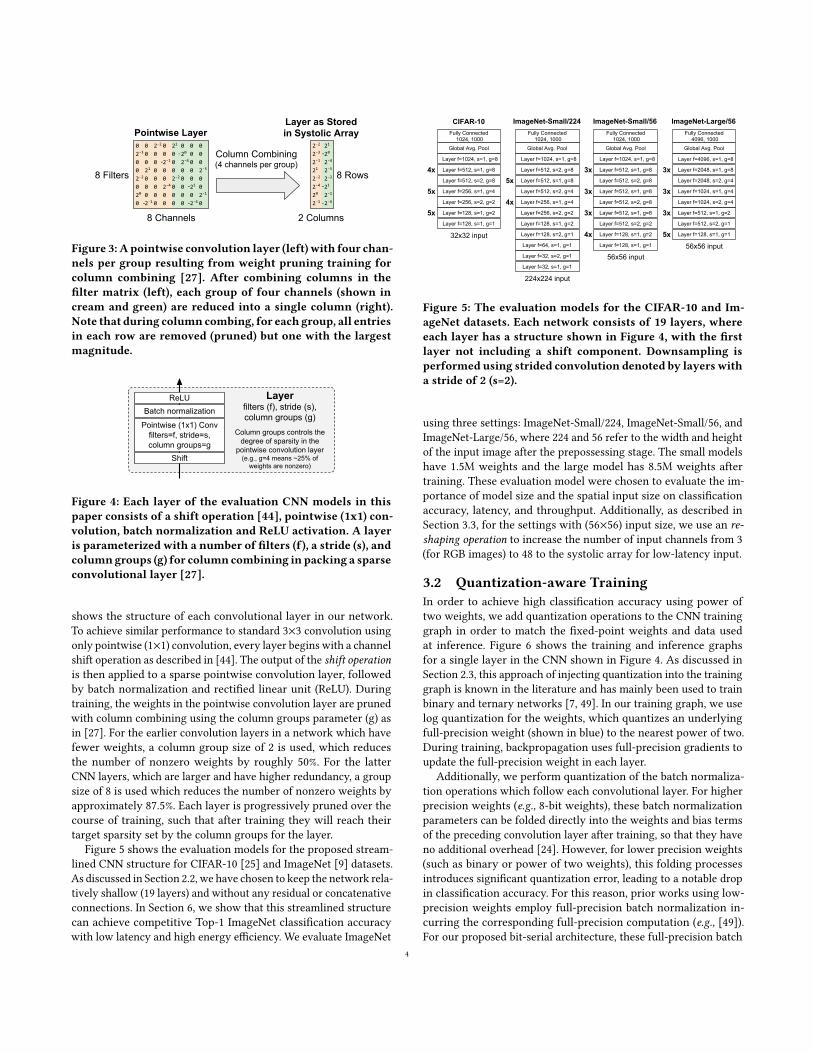
shows the structure of each convolutional layer in our network.To achieve similar performance to standard 3×3 convolution usingonly pointwise (1×1) convolution, every layer begins with a channelshift operation as described in [44]. The output of the shift operationis then applied to a sparse pointwise convolution layer, followedby batch normalization and rectified linear unit (ReLU). Duringtraining, the weights in the pointwise convolution layer are prunedwith column combining using the column groups parameter (g) asin [27]. For the earlier convolution layers in a network which havefewer weights, a column group size of 2 is used, which reducesthe number of nonzero weights by roughly 50%. For the latterCNN layers, which are larger and have higher redundancy, a groupsize of 8 is used which reduces the number of nonzero weights byapproximately 87.5%. Each layer is progressively pruned over thecourse of training, such that after training they will reach theirtarget sparsity set by the column groups for the layer.
Figure 5 shows the evaluation models for the proposed stream-lined CNN structure for CIFAR-10 [25] and ImageNet [9] datasets.As discussed in Section 2.2, we have chosen to keep the network rela-tively shallow (19 layers) and without any residual or concatenativeconnections. In Section 6, we show that this streamlined structurecan achieve competitive Top-1 ImageNet classification accuracywith low latency and high energy efficiency. We evaluate ImageNet
CIFAR-10 ImageNet-Small/224
Layer f=128, s=1, g=1
Layer f=128, s=1, g=24xLayer f=512, s=2, g=2
Layer f=512, s=1, g=83xLayer f=512, s=2, g=8
Layer f=512, s=1, g=83xLayer f=512, s=2, g=8
Layer f=512, s=1, g=83xLayer f=1024, s=1, g=8
Global Avg. Pool
Fully Connected 1024, 1000
Layer f=128, s=1, g=15xLayer f=512, s=2, g=1
Layer f=512, s=1, g=23x
3x
3xLayer f=4096, s=1, g=8
Global Avg. Pool
Fully Connected 4096, 1000
Layer f=1024, s=2, g=4
Layer f=1024, s=1, g=4
Layer f=2048, s=2, g=4
Layer f=2048, s=1, g=8
Layer f=128, s=1, g=2
Layer f=256, s=1, g=4
Layer f=512, s=2, g=4
4x
Layer f=512, s=1, g=8
Layer f=512, s=2, g=8
5x
Layer f=1024, s=1, g=8
Global Avg. Pool
Fully Connected 1024, 1000
Layer f=32, s=1, g=1
Layer f=32, s=2, g=1
Layer f=64, s=1, g=1
Layer f=128, s=2, g=1
Layer f=256, s=2, g=2
Layer f=128, s=1, g=1
Layer f=128, s=1, g=25xLayer f=256, s=2, g=2
Layer f=256, s=1, g=45xLayer f=512, s=2, g=8
Layer f=512, s=1, g=84x
Global Avg. Pool
Fully Connected 1024, 1000
Layer f=1024, s=1, g=8
32x32 input
224x224 input
56x56 input56x56 input
ImageNet-Small/56 ImageNet-Large/56
Figure 5: The evaluation models for the CIFAR-10 and Im-ageNet datasets. Each network consists of 19 layers, whereeach layer has a structure shown in Figure 4, with the firstlayer not including a shift component. Downsampling isperformed using strided convolution denoted by layers witha stride of 2 (s=2).
using three settings: ImageNet-Small/224, ImageNet-Small/56, andImageNet-Large/56, where 224 and 56 refer to the width and heightof the input image after the prepossessing stage. The small modelshave 1.5M weights and the large model has 8.5M weights aftertraining. These evaluation model were chosen to evaluate the im-portance of model size and the spatial input size on classificationaccuracy, latency, and throughput. Additionally, as described inSection 3.3, for the settings with (56×56) input size, we use an re-shaping operation to increase the number of input channels from 3(for RGB images) to 48 to the systolic array for low-latency input.
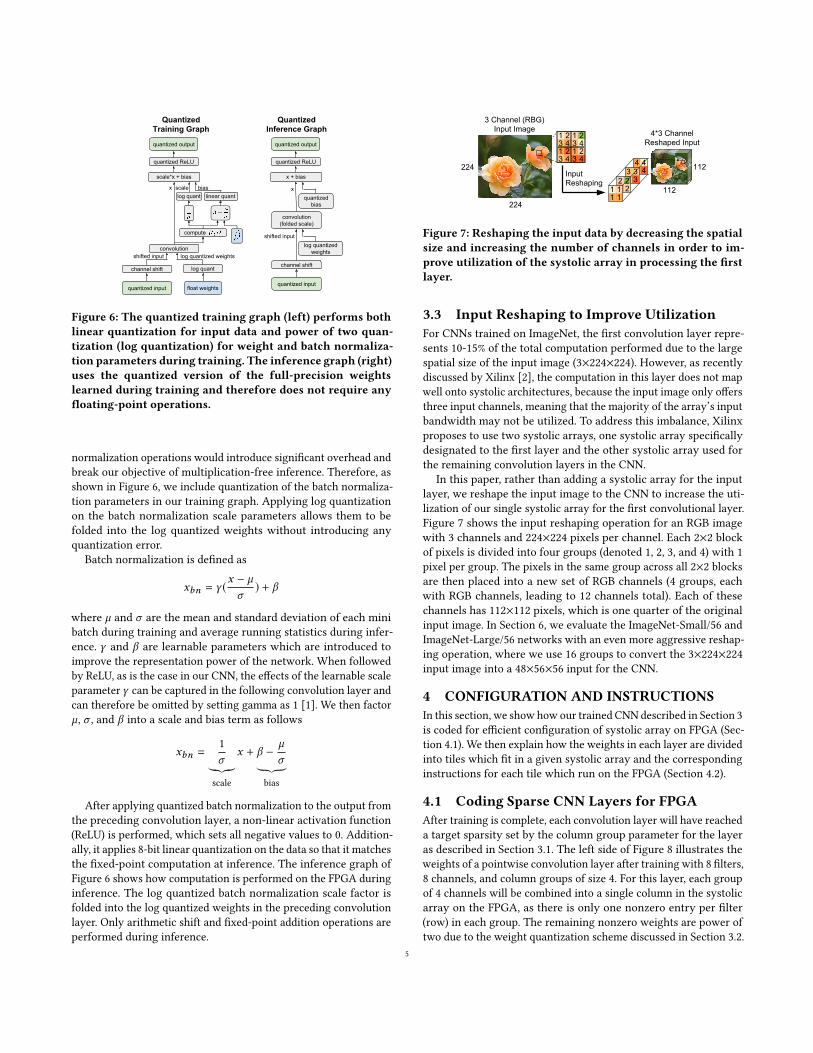
3.2 Quantization-aware TrainingIn order to achieve high classification accuracy using power oftwo weights, we add quantization operations to the CNN traininggraph in order to match the fixed-point weights and data usedat inference. Figure 6 shows the training and inference graphsfor a single layer in the CNN shown in Figure 4. As discussed inSection 2.3, this approach of injecting quantization into the traininggraph is known in the literature and has mainly been used to trainbinary and ternary networks [7, 49]. In our training graph, we uselog quantization for the weights, which quantizes an underlyingfull-precision weight (shown in blue) to the nearest power of two.During training, backpropagation uses full-precision gradients toupdate the full-precision weight in each layer.
Additionally, we perform quantization of the batch normaliza-tion operations which follow each convolutional layer. For higherprecision weights (e.g., 8-bit weights), these batch normalizationparameters can be folded directly into the weights and bias termsof the preceding convolution layer after training, so that they haveno additional overhead [24]. However, for lower precision weights(such as binary or power of two weights), this folding processesintroduces significant quantization error, leading to a notable dropin classification accuracy. For this reason, prior works using low-precision weights employ full-precision batch normalization in-curring the corresponding full-precision computation (e.g., [49]).For our proposed bit-serial architecture, these full-precision batch
4
QuantizedTraining Graph
float weights
log quant
quantized input
quantized output
channel shift
convolutionlog quantized weightsshifted input
compute
log quant
quantized ReLU
linear quantbiasscalex
scale*x + bias
QuantizedInference Graph
log quantized weights
quantized input
quantized output
channel shift
convolution (folded scale)
shifted input
x
x + bias
quantized bias
quantized ReLU
Figure 6: The quantized training graph (left) performs bothlinear quantization for input data and power of two quan-tization (log quantization) for weight and batch normaliza-tion parameters during training. The inference graph (right)uses the quantized version of the full-precision weightslearned during training and therefore does not require anyfloating-point operations.
normalization operations would introduce significant overhead andbreak our objective of multiplication-free inference. Therefore, asshown in Figure 6, we include quantization of the batch normaliza-tion parameters in our training graph. Applying log quantizationon the batch normalization scale parameters allows them to befolded into the log quantized weights without introducing anyquantization error.
Batch normalization is defined as
xbn = γ (x − µ
σ) + β
where µ and σ are the mean and standard deviation of each minibatch during training and average running statistics during infer-ence. γ and β are learnable parameters which are introduced toimprove the representation power of the network. When followedby ReLU, as is the case in our CNN, the effects of the learnable scaleparameter γ can be captured in the following convolution layer andcan therefore be omitted by setting gamma as 1 [1]. We then factorµ, σ , and β into a scale and bias term as follows
xbn =1σ︸︷︷︸
scale
x + β − µ
σ︸︷︷︸bias
After applying quantized batch normalization to the output fromthe preceding convolution layer, a non-linear activation function(ReLU) is performed, which sets all negative values to 0. Addition-ally, it applies 8-bit linear quantization on the data so that it matchesthe fixed-point computation at inference. The inference graph ofFigure 6 shows how computation is performed on the FPGA duringinference. The log quantized batch normalization scale factor isfolded into the log quantized weights in the preceding convolutionlayer. Only arithmetic shift and fixed-point addition operations areperformed during inference.
224
224
1 2 1 23 4 3 41 2 1 23 4 3 4
3 Channel (RBG) Input Image
112
112
4 44 43 3
3 32 22 21 1
1 1
4*3 Channel Reshaped Input
InputReshaping
Figure 7: Reshaping the input data by decreasing the spatialsize and increasing the number of channels in order to im-prove utilization of the systolic array in processing the firstlayer.
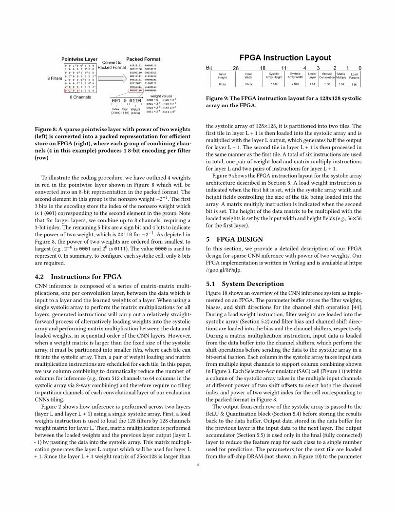
3.3 Input Reshaping to Improve UtilizationFor CNNs trained on ImageNet, the first convolution layer repre-sents 10-15% of the total computation performed due to the largespatial size of the input image (3×224×224). However, as recentlydiscussed by Xilinx [2], the computation in this layer does not mapwell onto systolic architectures, because the input image only offersthree input channels, meaning that the majority of the array’s inputbandwidth may not be utilized. To address this imbalance, Xilinxproposes to use two systolic arrays, one systolic array specificallydesignated to the first layer and the other systolic array used forthe remaining convolution layers in the CNN.
In this paper, rather than adding a systolic array for the inputlayer, we reshape the input image to the CNN to increase the uti-lization of our single systolic array for the first convolutional layer.Figure 7 shows the input reshaping operation for an RGB imagewith 3 channels and 224×224 pixels per channel. Each 2×2 blockof pixels is divided into four groups (denoted 1, 2, 3, and 4) with 1pixel per group. The pixels in the same group across all 2×2 blocksare then placed into a new set of RGB channels (4 groups, eachwith RGB channels, leading to 12 channels total). Each of thesechannels has 112×112 pixels, which is one quarter of the originalinput image. In Section 6, we evaluate the ImageNet-Small/56 andImageNet-Large/56 networks with an even more aggressive reshap-ing operation, where we use 16 groups to convert the 3×224×224input image into a 48×56×56 input for the CNN.
4 CONFIGURATION AND INSTRUCTIONSIn this section, we show how our trained CNN described in Section 3is coded for efficient configuration of systolic array on FPGA (Sec-tion 4.1). We then explain how the weights in each layer are dividedinto tiles which fit in a given systolic array and the correspondinginstructions for each tile which run on the FPGA (Section 4.2).
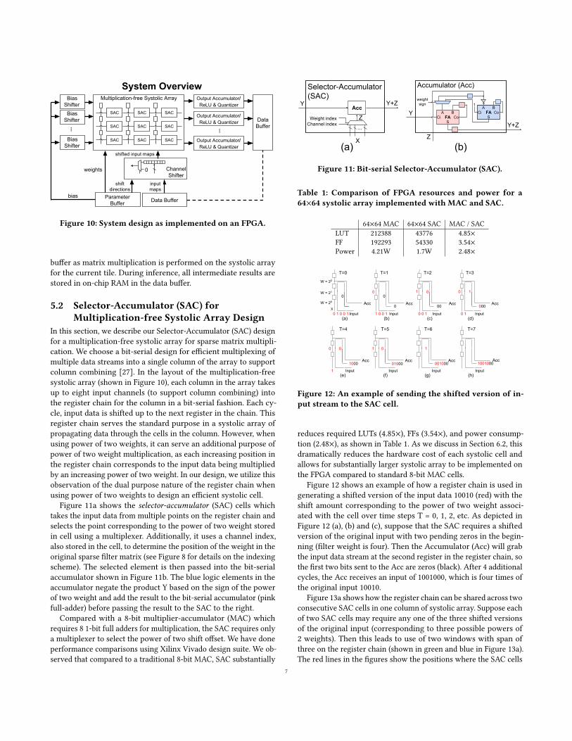
4.1 Coding Sparse CNN Layers for FPGAAfter training is complete, each convolution layer will have reacheda target sparsity set by the column group parameter for the layeras described in Section 3.1. The left side of Figure 8 illustrates theweights of a pointwise convolution layer after training with 8 filters,8 channels, and column groups of size 4. For this layer, each groupof 4 channels will be combined into a single column in the systolicarray on the FPGA, as there is only one nonzero entry per filter(row) in each group. The remaining nonzero weights are power oftwo due to the weight quantization scheme discussed in Section 3.2.
5
8 Filters
8 Channels
0 0 2-2 0 20 0 0 0
2-3 0 0 0 0 20 0 0
0 0 0 2-1 0 2-4 0 0
0 20 0 0 0 0 0 2-5
2-2 0 0 0 2-2 0 0 0
0 0 0 2-4 0 0 20 0
20 0 0 0 0 0 0 2-1
0 2-1 0 0 0 0 0
-
-
-
-
Convert toPacked Format 01010101 00000111
00010100 00110111
01100110 00110011
00110111 01110010
00010101 00000101
01110011 01000111
00010111 01110110
00100110 00000000
Packed Format
001 0 0110
Sign(1 bit)
Weight(4 bits)
Index(3 bits)
Pointwise Layer
0000 = 0 0001 = 2-6
0010 = 2-5
0011 = 2-4
weight values0100 = 2-3
0101 = 2-2
0110 = 2-1
0111 = 20
-
0
Figure 8: A sparse pointwise layerwith power of twoweights(left) is converted into a packed representation for efficientstore on FPGA (right), where each group of combining chan-nels (4 in this example) produces 1 8-bit encoding per filter(row).
To illustrate the coding procedure, we have outlined 4 weightsin red in the pointwise layer shown in Figure 8 which will beconverted into an 8-bit representation in the packed format. Thesecond element in this group is the nonzero weight −2−1. The first3 bits in the encoding store the index of the nonzero weight whichis 1 (001) corresponding to the second element in the group. Notethat for larger layers, we combine up to 8 channels, requiring a3-bit index. The remaining 5 bits are a sign bit and 4 bits to indicatethe power of two weight, which is 00110 for −2−1. As depicted inFigure 8, the power of two weights are ordered from smallest tolargest (e.g., 2−6 is 0001 and 20 is 0111). The value 0000 is used torepresent 0. In summary, to configure each systolic cell, only 8 bitsare required.
4.2 Instructions for FPGACNN inference is composed of a series of matrix-matrix multi-plications, one per convolution layer, between the data which isinput to a layer and the learned weights of a layer. When using asingle systolic array to perform the matrix multiplications for alllayers, generated instructions will carry out a relatively straight-forward process of alternatively loading weights into the systolicarray and performing matrix multiplication between the data andloaded weights, in sequential order of the CNN layers. However,when a weight matrix is larger than the fixed size of the systolicarray, it must be partitioned into smaller tiles, where each tile canfit into the systolic array. Then, a pair of weight loading and matrixmultiplication instructions are scheduled for each tile. In this paper,we use column combining to dramatically reduce the number ofcolumns for inference (e.g., from 512 channels to 64 columns in thesystolic array via 8-way combining) and therefore require no tilingto partition channels of each convolutional layer of our evaluationCNNs tiling.
Figure 2 shows how inference is performed across two layers(layer L and layer L + 1) using a single systolic array. First, a loadweights instruction is used to load the 128 filters by 128 channelsweight matrix for layer L. Then, matrix multiplication is performedbetween the loaded weights and the previous layer output (layer L- 1) by passing the data into the systolic array. This matrix multipli-cation generates the layer L output which will be used for layer L+ 1. Since the layer L + 1 weight matrix of 256×128 is larger than
Strided Convolution
1 bit
FPGA Instruction Layout
LoadParams
1 bit
MatrixMultiply
1 bit
SystolicArray Width
7 bits
SystolicArray Height
7 bits
InputWidth
8 bits
Linear Layer
1 bit
1 0211BitInput
Height
8 bits
341826
Figure 9: The FPGA instruction layout for a 128x128 systolicarray on the FPGA.
the systolic array of 128×128, it is partitioned into two tiles. Thefirst tile in layer L + 1 is then loaded into the systolic array and ismultiplied with the layer L output, which generates half the outputfor layer L + 1. The second tile in layer L + 1 is then processed inthe same manner as the first tile. A total of six instructions are usedin total, one pair of weight load and matrix multiply instructionsfor layer L and two pairs of instructions for layer L + 1.
Figure 9 shows the FPGA instruction layout for the systolic arrayarchitecture described in Section 5. A load weight instruction isindicated when the first bit is set, with the systolic array width andheight fields controlling the size of the tile being loaded into thearray. A matrix multiply instruction is indicated when the secondbit is set. The height of the data matrix to be multiplied with theloadedweights is set by the input width and height fields (e.g., 56×56for the first layer).
5 FPGA DESIGNIn this section, we provide a detailed description of our FPGAdesign for sparse CNN inference with power of two weights. OurFPGA implementation is written in Verilog and is available at https://goo.gl/8i9aJp.
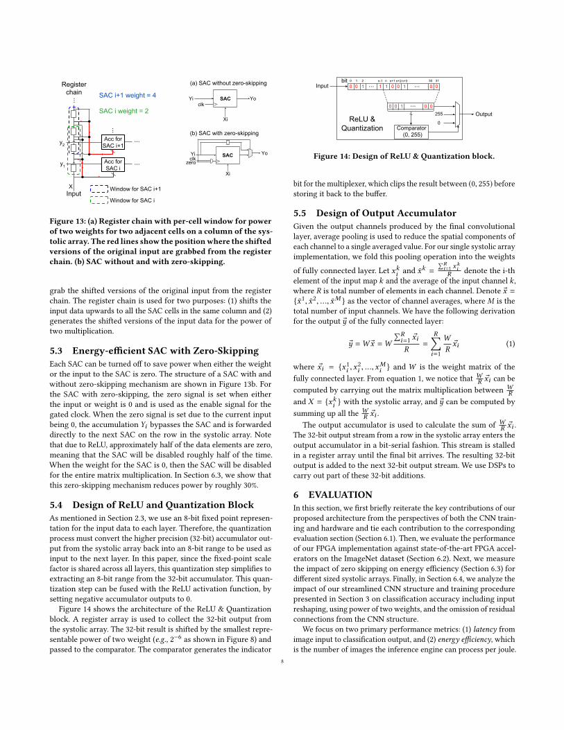
5.1 System DescriptionFigure 10 shows an overview of the CNN inference system as imple-mented on an FPGA. The parameter buffer stores the filter weights,biases, and shift directions for the channel shift operation [44].During a load weight instruction, filter weights are loaded into thesystolic array (Section 5.2) and filter bias and channel shift direc-tions are loaded into the bias and the channel shifters, respectively.During a matrix multiplication instruction, input data is loadedfrom the data buffer into the channel shifters, which perform theshift operations before sending the data to the systolic array in abit-serial fashion. Each column in the systolic array takes input datafrom multiple input channels to support column combining shownin Figure 3. Each Selector-Accumulator (SAC) cell (Figure 11) withina column of the systolic array takes in the multiple input channelsat different power of two shift offsets to select both the channelindex and power of two weight index for the cell corresponding tothe packed format in Figure 8.
The output from each row of the systolic array is passed to theReLU & Quantization block (Section 5.4) before storing the resultsback to the data buffer. Output data stored in the data buffer forthe previous layer is the input data to the next layer. The outputaccumulator (Section 5.5) is used only in the final (fully connected)layer to reduce the feature map for each class to a single numberused for prediction. The parameters for the next tile are loadedfrom the off-chip DRAM (not shown in Figure 10) to the parameter
6
DataBuffer
Channel Shifter
Multiplication-free Systolic Array
System Overview
Data BufferParameter Buffer
0
...
Bias Shifter
Bias Shifter
Bias Shifter
...
Output Accumulator/ ReLU & Quantizer
Output Accumulator/ ReLU & Quantizer
Output Accumulator/ ReLU & Quantizer
bias
weights
shift directions
inputmaps
shifted input maps
SAC
SAC
SAC
SAC
SAC
SAC
SAC SAC SAC
Figure 10: System design as implemented on an FPGA.
buffer as matrix multiplication is performed on the systolic arrayfor the current tile. During inference, all intermediate results arestored in on-chip RAM in the data buffer.
5.2 Selector-Accumulator (SAC) forMultiplication-free Systolic Array Design
In this section, we describe our Selector-Accumulator (SAC) designfor a multiplication-free systolic array for sparse matrix multipli-cation. We choose a bit-serial design for efficient multiplexing ofmultiple data streams into a single column of the array to supportcolumn combining [27]. In the layout of the multiplication-freesystolic array (shown in Figure 10), each column in the array takesup to eight input channels (to support column combining) intothe register chain for the column in a bit-serial fashion. Each cy-cle, input data is shifted up to the next register in the chain. Thisregister chain serves the standard purpose in a systolic array ofpropagating data through the cells in the column. However, whenusing power of two weights, it can serve an additional purpose ofpower of two weight multiplication, as each increasing position inthe register chain corresponds to the input data being multipliedby an increasing power of two weight. In our design, we utilize thisobservation of the dual purpose nature of the register chain whenusing power of two weights to design an efficient systolic cell.
Figure 11a shows the selector-accumulator (SAC) cells whichtakes the input data from multiple points on the register chain andselects the point corresponding to the power of two weight storedin cell using a multiplexer. Additionally, it uses a channel index,also stored in the cell, to determine the position of the weight in theoriginal sparse filter matrix (see Figure 8 for details on the indexingscheme). The selected element is then passed into the bit-serialaccumulator shown in Figure 11b. The blue logic elements in theaccumulator negate the product Y based on the sign of the powerof two weight and add the result to the bit-serial accumulator (pinkfull-adder) before passing the result to the SAC to the right.
Compared with a 8-bit multiplier-accumulator (MAC) whichrequires 8 1-bit full adders for multiplication, the SAC requires onlya multiplexer to select the power of two shift offset. We have doneperformance comparisons using Xilinx Vivado design suite. We ob-served that compared to a traditional 8-bit MAC, SAC substantially
Selector-Accumulator(SAC)
Acc
Z FACi CoA B
S
FACi CoB
S
1weight sign
A
Accumulator (Acc)
Z
Y
Y+Z
Y
Channel indexWeight index
...
X(a) (b)
Y+Z
Figure 11: Bit-serial Selector-Accumulator (SAC).
Table 1: Comparison of FPGA resources and power for a64×64 systolic array implemented with MAC and SAC.
64×64 MAC 64×64 SAC MAC / SACLUT 212388 43776 4.85×FF 192293 54330 3.54×Power 4.21W 1.7W 2.48×
Acc
AccAccAcc
Acc
Input1 0 0 1 Input 0 0 1 Input
0
0 1
1
Input
0
1 Input Input
1
T=1 T=2 T=3
T=6T=5T=4
00 000
001000 010001000
(b) (c) (d)
(g)(f)(e)
XInput0 1 0 0 1
T=0
(a)
Input
T=7
1001000
(h)
0
W = 22
W = 21
W = 20
0
Acc
Acc
Acc0
00 1
0 0 1
Figure 12: An example of sending the shifted version of in-put stream to the SAC cell.
reduces required LUTs (4.85×), FFs (3.54×), and power consump-tion (2.48×), as shown in Table 1. As we discuss in Section 6.2, thisdramatically reduces the hardware cost of each systolic cell andallows for substantially larger systolic array to be implemented onthe FPGA compared to standard 8-bit MAC cells.
Figure 12 shows an example of how a register chain is used ingenerating a shifted version of the input data 10010 (red) with theshift amount corresponding to the power of two weight associ-ated with the cell over time steps T = 0, 1, 2, etc. As depicted inFigure 12 (a), (b) and (c), suppose that the SAC requires a shiftedversion of the original input with two pending zeros in the begin-ning (filter weight is four). Then the Accumulator (Acc) will grabthe input data stream at the second register in the register chain, sothe first two bits sent to the Acc are zeros (black). After 4 additionalcycles, the Acc receives an input of 1001000, which is four times ofthe original input 10010.
Figure 13a shows how the register chain can be shared across twoconsecutive SAC cells in one column of systolic array. Suppose eachof two SAC cells may require any one of the three shifted versionsof the original input (corresponding to three possible powers of2 weights). Then this leads to use of two windows with span ofthree on the register chain (shown in green and blue in Figure 13a).The red lines in the figures show the positions where the SAC cells
7
y1
y2
Register chain
...
...
...
...
XInput
Window for SAC i+1
Acc for SAC i+1
Acc for SAC i
Window for SAC i
SAC i+1 weight = 4
SAC i weight = 2
SACclkYi
zero
Yo
Xi
SAC
Xi
clkYi Yo
(a) SAC without zero-skipping
(b) SAC with zero-skipping
Figure 13: (a) Register chain with per-cell window for powerof two weights for two adjacent cells on a column of the sys-tolic array. The red lines show the positionwhere the shiftedversions of the original input are grabbed from the registerchain. (b) SAC without and with zero-skipping.
grab the shifted versions of the original input from the registerchain. The register chain is used for two purposes: (1) shifts theinput data upwards to all the SAC cells in the same column and (2)generates the shifted versions of the input data for the power oftwo multiplication.
5.3 Energy-efficient SAC with Zero-SkippingEach SAC can be turned off to save power when either the weightor the input to the SAC is zero. The structure of a SAC with andwithout zero-skipping mechanism are shown in Figure 13b. Forthe SAC with zero-skipping, the zero signal is set when eitherthe input or weight is 0 and is used as the enable signal for thegated clock. When the zero signal is set due to the current inputbeing 0, the accumulation Yi bypasses the SAC and is forwardeddirectly to the next SAC on the row in the systolic array. Notethat due to ReLU, approximately half of the data elements are zero,meaning that the SAC will be disabled roughly half of the time.When the weight for the SAC is 0, then the SAC will be disabledfor the entire matrix multiplication. In Section 6.3, we show thatthis zero-skipping mechanism reduces power by roughly 30%.
5.4 Design of ReLU and Quantization BlockAs mentioned in Section 2.3, we use an 8-bit fixed point represen-tation for the input data to each layer. Therefore, the quantizationprocess must convert the higher precision (32-bit) accumulator out-put from the systolic array back into an 8-bit range to be used asinput to the next layer. In this paper, since the fixed-point scalefactor is shared across all layers, this quantization step simplifies toextracting an 8-bit range from the 32-bit accumulator. This quan-tization step can be fused with the ReLU activation function, bysetting negative accumulator outputs to 0.
Figure 14 shows the architecture of the ReLU & Quantizationblock. A register array is used to collect the 32-bit output fromthe systolic array. The 32-bit result is shifted by the smallest repre-sentable power of two weight (e.g., 2−6 as shown in Figure 8) andpassed to the comparator. The comparator generates the indicator
3100
bit0
30
ReLU&Quantization
101101100 ...
0 1011011
0 1 2 3 4 5 6 7 8 9
0 1
0
Comparator (0, )
8
Input
Output
31
00bit
030
ReLU &Quantization
1011100 ...
0 010 0
0 1 2 n-1 n n+1
0Comparator (0, 255)
Input
Output
...
n+2 n+3...
255
Figure 14: Design of ReLU & Quantization block.
bit for the multiplexer, which clips the result between (0, 255) beforestoring it back to the buffer.
5.5 Design of Output AccumulatorGiven the output channels produced by the final convolutionallayer, average pooling is used to reduce the spatial components ofeach channel to a single averaged value. For our single systolic arrayimplementation, we fold this pooling operation into the weights
of fully connected layer. Let xki and x̄k =∑Ri=1 x
ki
R denote the i-thelement of the input map k and the average of the input channel k ,where R is total number of elements in each channel. Denote ®x ={x̄1, x̄2, ..., x̄M } as the vector of channel averages, whereM is thetotal number of input channels. We have the following derivationfor the output ®y of the fully connected layer:
®y =W ®x =W∑Ri=1 ®xiR
=
R∑i=1
W
R®xi (1)
where ®xi = {x1i ,x
2i , ...,x
Mi } and W is the weight matrix of the
fully connected layer. From equation 1, we notice that WR ®xi can becomputed by carrying out the matrix multiplication between W
Rand X = {xki } with the systolic array, and ®y can be computed bysumming up all the W
R ®xi .The output accumulator is used to calculate the sum of W
R ®xi .The 32-bit output stream from a row in the systolic array enters theoutput accumulator in a bit-serial fashion. This stream is stalledin a register array until the final bit arrives. The resulting 32-bitoutput is added to the next 32-bit output stream. We use DSPs tocarry out part of these 32-bit additions.
6 EVALUATIONIn this section, we first briefly reiterate the key contributions of ourproposed architecture from the perspectives of both the CNN train-ing and hardware and tie each contribution to the correspondingevaluation section (Section 6.1). Then, we evaluate the performanceof our FPGA implementation against state-of-the-art FPGA accel-erators on the ImageNet dataset (Section 6.2). Next, we measurethe impact of zero skipping on energy efficiency (Section 6.3) fordifferent sized systolic arrays. Finally, in Section 6.4, we analyze theimpact of our streamlined CNN structure and training procedurepresented in Section 3 on classification accuracy including inputreshaping, using power of two weights, and the omission of residualconnections from the CNN structure.
We focus on two primary performance metrics: (1) latency fromimage input to classification output, and (2) energy efficiency, whichis the number of images the inference engine can process per joule.
8
Note that the latter is also the number of images/sec (i.e., through-put) per watt. For high-throughput inference applications we mayuse multiple inference engines in parallel. If these individual en-gines each offer low latency and high-energy efficient inference,then the aggregate system will delivery high-throughput inferencesper watt while meeting low inference latency requirements.
6.1 Recap of Full-stack OptimizationFull-stack optimization via training has enabled the following de-sign advances which lead to our efficient FPGA implementationpresented in Section 5.
• Using power of two for weights and the batch normalizationscale parameters, outlined in Section 2.3, for all layers in theCNN (including the fully connected layer). This allows for asimplified design, where a single sparse multiplication-freesystolic array is used for all CNN layers. In Section 6.4.2, wediscuss the impact of the proposed quantization scheme onclassification accuracy.
• Zero-skipping of the quantized data (Section 5.3). In Sec-tion 6.3, we show that zero-skipping reduces the power con-sumption during matrix multiplication by roughly 30%.
• Packing sparse CNNs using column combining [27] for ef-ficient storage and use on FPGAs, which we describe inSection 4.1. Our ImageNet-Small/56 evaluation model hasonly 1.5M power of two weights, which is 40× smaller thanAlexNet and 92× smaller than VGG-16 (the two CNNs usedby other FPGA designs).
• Using channel shifts [44] to replace 3×3 convolutions with1×1 convolutions. As with column combining, this reducesthe number of model parameters. Additionally, it streamlinesthe design of the systolic array system, as 1×1 reduces tomatrix multiplication.
• Input reshaping (Section 3.3) to increase the bit-serial sys-tolic array utilization and dramatically reduce the latencyfor the first convolution layer. In Section 6.4.1, we show thatinput reshaping alleviates the accuracy loss when using asmaller spatial input size of 56×56 instead of the conven-tional 224×224.
6.2 Comparing to Prior FPGA AcceleratorsWe compare our 170 MHz FPGA design to several state-of-the-art FPGA accelerators on the ImageNet dataset in terms of top-1classification accuracy, latency for a single input image, and energyefficiency when no batch processing is performed (i.e., batch sizeof 1). By choosing these metrics, we focus on real-time scenarioswhere input samples must be processed immediately to meet a hardtime constraint. Our evaluation model is the ImageNet-Small/56network shown in Figure 5 with input reshaping to 48×56×56. OurFPGA can fit a systolic array of size 128 rows by 64 columns. Eachof the columns can span up to 8 channels in convolution weightmatrix, i.e., when the column group parameter is set to 8, for a totalof 512 channels.
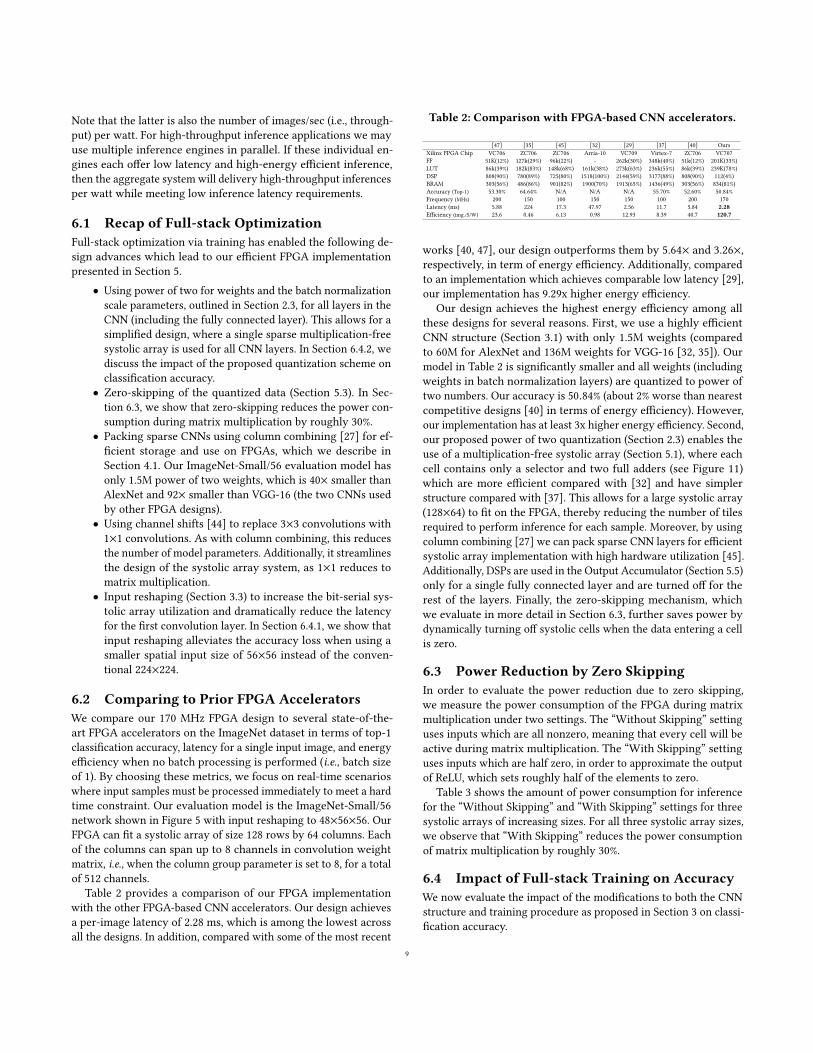
Table 2 provides a comparison of our FPGA implementationwith the other FPGA-based CNN accelerators. Our design achievesa per-image latency of 2.28 ms, which is among the lowest acrossall the designs. In addition, compared with some of the most recent
Table 2: Comparison with FPGA-based CNN accelerators.
[47] [35] [45] [32] [29] [37] [40] OursXilinx FPGA Chip VC706 ZC706 ZC706 Arria-10 VC709 Virtex-7 ZC706 VC707FF 51K(12%) 127k(29%) 96k(22%) - 262k(30%) 348k(40%) 51k(12%) 201K(33%)LUT 86k(39%) 182k(83%) 148k(68%) 161k(38%) 273k(63%) 236k(55%) 86k(39%) 239K(78%)DSP 808(90%) 780(89%) 725(80%) 1518(100%) 2144(59%) 3177(88%) 808(90%) 112(4%)BRAM 303(56%) 486(86%) 901(82%) 1900(70%) 1913(65%) 1436(49%) 303(56%) 834(81%)Accuracy (Top-1) 53.30% 64.64% N/A N/A N/A 55.70% 52.60% 50.84%Frequency (MHz) 200 150 100 150 150 100 200 170Latency (ms) 5.88 224 17.3 47.97 2.56 11.7 5.84 2.28Efficiency (img./S/W) 23.6 0.46 6.13 0.98 12.93 8.39 40.7 120.7
works [40, 47], our design outperforms them by 5.64× and 3.26×,respectively, in term of energy efficiency. Additionally, comparedto an implementation which achieves comparable low latency [29],our implementation has 9.29x higher energy efficiency.
Our design achieves the highest energy efficiency among allthese designs for several reasons. First, we use a highly efficientCNN structure (Section 3.1) with only 1.5M weights (comparedto 60M for AlexNet and 136M weights for VGG-16 [32, 35]). Ourmodel in Table 2 is significantly smaller and all weights (includingweights in batch normalization layers) are quantized to power oftwo numbers. Our accuracy is 50.84% (about 2% worse than nearestcompetitive designs [40] in terms of energy efficiency). However,our implementation has at least 3x higher energy efficiency. Second,our proposed power of two quantization (Section 2.3) enables theuse of a multiplication-free systolic array (Section 5.1), where eachcell contains only a selector and two full adders (see Figure 11)which are more efficient compared with [32] and have simplerstructure compared with [37]. This allows for a large systolic array(128×64) to fit on the FPGA, thereby reducing the number of tilesrequired to perform inference for each sample. Moreover, by usingcolumn combining [27] we can pack sparse CNN layers for efficientsystolic array implementation with high hardware utilization [45].Additionally, DSPs are used in the Output Accumulator (Section 5.5)only for a single fully connected layer and are turned off for therest of the layers. Finally, the zero-skipping mechanism, whichwe evaluate in more detail in Section 6.3, further saves power bydynamically turning off systolic cells when the data entering a cellis zero.
6.3 Power Reduction by Zero SkippingIn order to evaluate the power reduction due to zero skipping,we measure the power consumption of the FPGA during matrixmultiplication under two settings. The “Without Skipping” settinguses inputs which are all nonzero, meaning that every cell will beactive during matrix multiplication. The “With Skipping” settinguses inputs which are half zero, in order to approximate the outputof ReLU, which sets roughly half of the elements to zero.
Table 3 shows the amount of power consumption for inferencefor the “Without Skipping” and “With Skipping” settings for threesystolic arrays of increasing sizes. For all three systolic array sizes,we observe that “With Skipping” reduces the power consumptionof matrix multiplication by roughly 30%.
6.4 Impact of Full-stack Training on AccuracyWe now evaluate the impact of the modifications to both the CNNstructure and training procedure as proposed in Section 3 on classi-fication accuracy.
9
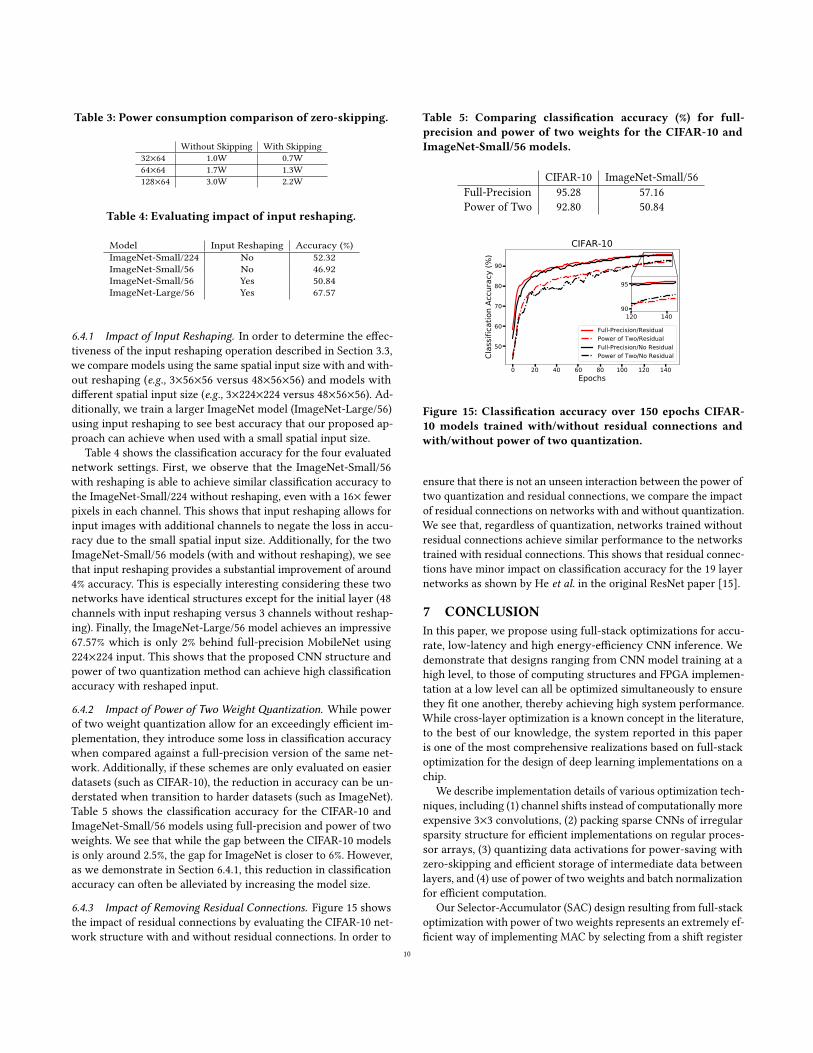
Table 3: Power consumption comparison of zero-skipping.
Without Skipping With Skipping32×64 1.0W 0.7W64×64 1.7W 1.3W128×64 3.0W 2.2W
Table 4: Evaluating impact of input reshaping.
Model Input Reshaping Accuracy (%)ImageNet-Small/224 No 52.32ImageNet-Small/56 No 46.92ImageNet-Small/56 Yes 50.84ImageNet-Large/56 Yes 67.57
6.4.1 Impact of Input Reshaping. In order to determine the effec-tiveness of the input reshaping operation described in Section 3.3,we compare models using the same spatial input size with and with-out reshaping (e.g., 3×56×56 versus 48×56×56) and models withdifferent spatial input size (e.g., 3×224×224 versus 48×56×56). Ad-ditionally, we train a larger ImageNet model (ImageNet-Large/56)using input reshaping to see best accuracy that our proposed ap-proach can achieve when used with a small spatial input size.
Table 4 shows the classification accuracy for the four evaluatednetwork settings. First, we observe that the ImageNet-Small/56with reshaping is able to achieve similar classification accuracy tothe ImageNet-Small/224 without reshaping, even with a 16× fewerpixels in each channel. This shows that input reshaping allows forinput images with additional channels to negate the loss in accu-racy due to the small spatial input size. Additionally, for the twoImageNet-Small/56 models (with and without reshaping), we seethat input reshaping provides a substantial improvement of around4% accuracy. This is especially interesting considering these twonetworks have identical structures except for the initial layer (48channels with input reshaping versus 3 channels without reshap-ing). Finally, the ImageNet-Large/56 model achieves an impressive67.57% which is only 2% behind full-precision MobileNet using224×224 input. This shows that the proposed CNN structure andpower of two quantization method can achieve high classificationaccuracy with reshaped input.
6.4.2 Impact of Power of Two Weight Quantization. While powerof two weight quantization allow for an exceedingly efficient im-plementation, they introduce some loss in classification accuracywhen compared against a full-precision version of the same net-work. Additionally, if these schemes are only evaluated on easierdatasets (such as CIFAR-10), the reduction in accuracy can be un-derstated when transition to harder datasets (such as ImageNet).Table 5 shows the classification accuracy for the CIFAR-10 andImageNet-Small/56 models using full-precision and power of twoweights. We see that while the gap between the CIFAR-10 modelsis only around 2.5%, the gap for ImageNet is closer to 6%. However,as we demonstrate in Section 6.4.1, this reduction in classificationaccuracy can often be alleviated by increasing the model size.
6.4.3 Impact of Removing Residual Connections. Figure 15 showsthe impact of residual connections by evaluating the CIFAR-10 net-work structure with and without residual connections. In order to
Table 5: Comparing classification accuracy (%) for full-precision and power of two weights for the CIFAR-10 andImageNet-Small/56 models.
CIFAR-10 ImageNet-Small/56Full-Precision 95.28 57.16Power of Two 92.80 50.84
0 20 40 60 80 100 120 140Epochs
50
60
70
80
90
Clas
sifica
tion
Accu
racy
(%)
CIFAR-10
Full-Precision/ResidualPower of Two/ResidualFull-Precision/No ResidualPower of Two/No Residual
120 14090
95
Figure 15: Classification accuracy over 150 epochs CIFAR-10 models trained with/without residual connections andwith/without power of two quantization.
ensure that there is not an unseen interaction between the power oftwo quantization and residual connections, we compare the impactof residual connections on networks with and without quantization.We see that, regardless of quantization, networks trained withoutresidual connections achieve similar performance to the networkstrained with residual connections. This shows that residual connec-tions have minor impact on classification accuracy for the 19 layernetworks as shown by He et al. in the original ResNet paper [15].
7 CONCLUSIONIn this paper, we propose using full-stack optimizations for accu-rate, low-latency and high energy-efficiency CNN inference. Wedemonstrate that designs ranging from CNN model training at ahigh level, to those of computing structures and FPGA implemen-tation at a low level can all be optimized simultaneously to ensurethey fit one another, thereby achieving high system performance.While cross-layer optimization is a known concept in the literature,to the best of our knowledge, the system reported in this paperis one of the most comprehensive realizations based on full-stackoptimization for the design of deep learning implementations on achip.
We describe implementation details of various optimization tech-niques, including (1) channel shifts instead of computationally moreexpensive 3×3 convolutions, (2) packing sparse CNNs of irregularsparsity structure for efficient implementations on regular proces-sor arrays, (3) quantizing data activations for power-saving withzero-skipping and efficient storage of intermediate data betweenlayers, and (4) use of power of two weights and batch normalizationfor efficient computation.
Our Selector-Accumulator (SAC) design resulting from full-stackoptimization with power of two weights represents an extremely ef-ficient way of implementing MAC by selecting from a shift register
10
rather than performing arithmetic operations. (It would be difficultto have a more efficient MAC design, short of analog implementa-tions!) Given that MAC is the basic operation in the dot-productcomputation for matching data against filters, we believe our SACresult is significant.
REFERENCES[1] [n. d.]. Functional interface for the batch normalization layer. https://www.
tensorflow.org/api_docs/python/tf/layers/batch_normalization. ([n. d.]). Ac-cessed: 2018-12-04.
[2] 2018. Accelerating DNNs with Xilinx Alveo Accelerator Cards. Technical Report.Xilinx.
[3] Manoj Alwani, Han Chen, Michael Ferdman, and Peter Milder. 2016. Fused-layerCNN accelerators. In The 49th Annual IEEE/ACM International Symposium onMicroarchitecture. IEEE Press, 22.
[4] Zhaowei Cai, Xiaodong He, Jian Sun, and Nuno Vasconcelos. 2017. Deep learn-ing with low precision by half-wave gaussian quantization. arXiv preprintarXiv:1702.00953 (2017).
[5] Jungwook Choi, Zhuo Wang, Swagath Venkataramani, Pierce I-Jen Chuang,Vijayalakshmi Srinivasan, and Kailash Gopalakrishnan. 2018. PACT: Param-eterized Clipping Activation for Quantized Neural Networks. arXiv preprintarXiv:1805.06085 (2018).
[6] François Chollet. 2016. Xception: Deep Learning with Depthwise SeparableConvolutions. arXiv preprint arXiv:1610.02357 (2016).
[7] Matthieu Courbariaux, Yoshua Bengio, and Jean-Pierre David. 2015. Binarycon-nect: Training deep neural networks with binary weights during propagations.In Advances in neural information processing systems. 3123–3131.
[8] Matthieu Courbariaux, Itay Hubara, Daniel Soudry, Ran El-Yaniv, and YoshuaBengio. 2016. Binarized neural networks: Training deep neural networks withweights and activations constrained to+ 1 or-1. arXiv preprint arXiv:1602.02830(2016).
[9] Jia Deng, Wei Dong, Richard Socher, Li-Jia Li, Kai Li, and Li Fei-Fei. 2009. Ima-genet: A large-scale hierarchical image database. In Computer Vision and PatternRecognition, 2009. CVPR 2009. IEEE Conference on. IEEE, 248–255.
[10] Tim Dettmers. 2015. 8-bit approximations for parallelism in deep learning. arXivpreprint arXiv:1511.04561 (2015).
[11] Zidong Du, Robert Fasthuber, Tianshi Chen, Paolo Ienne, Ling Li, Tao Luo,Xiaobing Feng, Yunji Chen, and Olivier Temam. 2015. ShiDianNao: Shiftingvision processing closer to the sensor. In ACM SIGARCH Computer ArchitectureNews, Vol. 43. ACM, 92–104.
[12] Scott Gray, Alec Radford, and Diederik Kingma. 2017. GPU Kernels forBlock-Sparse Weights. https://s3-us-west-2.amazonaws.com/openai-assets/blocksparse/blocksparsepaper.pdf. (2017). [Online; accessed 12-January-2018].
[13] Suyog Gupta, Ankur Agrawal, Kailash Gopalakrishnan, and Pritish Narayanan.2015. Deep learning with limited numerical precision. In International Conferenceon Machine Learning. 1737–1746.
[14] Song Han, Huizi Mao, andWilliam J Dally. 2015. Deep compression: Compressingdeep neural networks with pruning, trained quantization and huffman coding.arXiv preprint arXiv:1510.00149 (2015).
[15] Kaiming He, Xiangyu Zhang, Shaoqing Ren, and Jian Sun. 2016. Deep residuallearning for image recognition. In Proceedings of the IEEE conference on computervision and pattern recognition. 770–778.
[16] Yihui He, Xiangyu Zhang, and Jian Sun. 2017. Channel pruning for acceleratingvery deep neural networks. In International Conference on Computer Vision (ICCV),Vol. 2.
[17] Andrew G Howard, Menglong Zhu, Bo Chen, Dmitry Kalenichenko, WeijunWang, Tobias Weyand, Marco Andreetto, and Hartwig Adam. 2017. Mobilenets:Efficient convolutional neural networks for mobile vision applications. arXivpreprint arXiv:1704.04861 (2017).
[18] Qinghao Hu, Peisong Wang, and Jian Cheng. 2018. From hashing to CNNs:Training BinaryWeight networks via hashing. arXiv preprint arXiv:1802.02733(2018).
[19] Gao Huang, Shichen Liu, Laurens van der Maaten, and Kilian QWeinberger. 2017.CondenseNet: An Efficient DenseNet using Learned Group Convolutions. arXivpreprint arXiv:1711.09224 (2017).
[20] Gao Huang, Zhuang Liu, Laurens Van Der Maaten, and Kilian Q Weinberger.2017. Densely connected convolutional networks.. In CVPR, Vol. 1. 3.
[21] Sergey Ioffe and Christian Szegedy. 2015. Batch normalization: Acceleratingdeep network training by reducing internal covariate shift. arXiv preprintarXiv:1502.03167 (2015).
[22] Benoit Jacob, Skirmantas Kligys, Bo Chen,Menglong Zhu,MatthewTang, AndrewHoward, Hartwig Adam, and Dmitry Kalenichenko. [n. d.]. Quantization andtraining of neural networks for efficient integer-arithmetic-only inference. ([n.d.]).
[23] Norman P. Jouppi, Cliff Young, Nishant Patil, David Patterson, Gaurav Agrawal,Raminder Bajwa, Sarah Bates, Suresh Bhatia, Nan Boden, Al Borchers, Rick Boyle,Pierre-luc Cantin, Clifford Chao, Chris Clark, Jeremy Coriell, Mike Daley, MattDau, Jeffrey Dean, Ben Gelb, Tara Vazir Ghaemmaghami, Rajendra Gottipati,William Gulland, Robert Hagmann, C. Richard Ho, Doug Hogberg, John Hu,Robert Hundt, Dan Hurt, Julian Ibarz, Aaron Jaffey, Alek Jaworski, AlexanderKaplan, Harshit Khaitan, Daniel Killebrew, Andy Koch, Naveen Kumar, SteveLacy, James Laudon, James Law, Diemthu Le, Chris Leary, Zhuyuan Liu, KyleLucke, Alan Lundin, Gordon MacKean, Adriana Maggiore, Maire Mahony, KieranMiller, Rahul Nagarajan, Ravi Narayanaswami, Ray Ni, Kathy Nix, Thomas Norrie,Mark Omernick, Narayana Penukonda, Andy Phelps, Jonathan Ross, Matt Ross,Amir Salek, Emad Samadiani, Chris Severn, Gregory Sizikov, Matthew Snelham,Jed Souter, Dan Steinberg, Andy Swing, Mercedes Tan, Gregory Thorson, BoTian, Horia Toma, Erick Tuttle, Vijay Vasudevan, Richard Walter, Walter Wang,Eric Wilcox, and Doe Hyun Yoon. 2017. In-Datacenter Performance Analysisof a Tensor Processing Unit. In Proceedings of the 44th Annual InternationalSymposium on Computer Architecture (ISCA ’17). ACM, New York, NY, USA, 1–12.https://doi.org/10.1145/3079856.3080246
[24] Raghuraman Krishnamoorthi. 2018. Quantizing deep convolutional networksfor efficient inference: A whitepaper. arXiv preprint arXiv:1806.08342 (2018).
[25] Alex Krizhevsky, Vinod Nair, and Geoffrey Hinton. 2014. The CIFAR-10 dataset.(2014).
[26] Alex Krizhevsky, Ilya Sutskever, and Geoffrey E Hinton. 2012. Imagenet classifica-tion with deep convolutional neural networks. In Advances in neural informationprocessing systems. 1097–1105.
[27] H. T. Kung, Bradley McDanel, and Sai Qian Zhang. 2018. Packing Sparse Convo-lutional Neural Networks for Efficient Systolic Array Implementations: ColumnCombining Under Joint Optimization. arXiv preprint arXiv:1811.04770 (2018). Toappear in Proceedings of the 24th ACM International Conference on Architec-tural Support for Programming Languages and Operating Systems 2019 (ASPLOS2019).
[28] Yann LeCun, Léon Bottou, Yoshua Bengio, and Patrick Haffner. 1998. Gradient-based learning applied to document recognition. Proc. IEEE 86, 11 (1998), 2278–2324.
[29] Huimin Li, Xitian Fan, Li Jiao, Wei Cao, Xuegong Zhou, and Lingli Wang. 2016.A high performance FPGA-based accelerator for large-scale convolutional neuralnetworks. In Field Programmable Logic and Applications (FPL), 2016 26th Interna-tional Conference on. IEEE, 1–9.
[30] Zechun Liu, Baoyuan Wu, Wenhan Luo, Xin Yang, Wei Liu, and Kwang-TingCheng. 2018. Bi-real net: Enhancing the performance of 1-bit cnns with improvedrepresentational capability and advanced training algorithm. arXiv preprintarXiv:1808.00278 (2018).
[31] Jian-Hao Luo, Jianxin Wu, and Weiyao Lin. 2017. Thinet: A filter level pruningmethod for deep neural network compression. arXiv preprint arXiv:1707.06342(2017).
[32] Yufei Ma, Yu Cao, Sarma Vrudhula, and Jae-sun Seo. 2017. Optimizing loopoperation and dataflow in fpga acceleration of deep convolutional neural net-works. In Proceedings of the 2017 ACM/SIGDA International Symposium on Field-Programmable Gate Arrays. ACM, 45–54.
[33] Sharan Narang, Eric Undersander, and Gregory F. Diamos. 2017. Block-SparseRecurrent Neural Networks. CoRR abs/1711.02782 (2017). arXiv:1711.02782http://arxiv.org/abs/1711.02782
[34] Adam Paszke, Sam Gross, Soumith Chintala, Gregory Chanan, Edward Yang,Zachary DeVito, Zeming Lin, Alban Desmaison, Luca Antiga, and Adam Lerer.2017. Automatic differentiation in PyTorch. (2017).
[35] Jiantao Qiu, Jie Wang, Song Yao, Kaiyuan Guo, Boxun Li, Erjin Zhou, Jincheng Yu,Tianqi Tang, Ningyi Xu, Sen Song, et al. 2016. Going deeper with embedded fpgaplatform for convolutional neural network. In Proceedings of the 2016 ACM/SIGDAInternational Symposium on Field-Programmable Gate Arrays. ACM, 26–35.
[36] Mohammad Rastegari, Vicente Ordonez, Joseph Redmon, and Ali Farhadi. 2016.Xnor-net: Imagenet classification using binary convolutional neural networks.In European Conference on Computer Vision. Springer, 525–542.
[37] Yongming Shen, Michael Ferdman, and Peter Milder. 2017. Maximizing CNNaccelerator efficiency through resource partitioning. In Computer Architecture(ISCA), 2017 ACM/IEEE 44th Annual International Symposium on. IEEE, 535–547.
[38] Karen Simonyan and Andrew Zisserman. 2014. Very deep convolutional networksfor large-scale image recognition. arXiv preprint arXiv:1409.1556 (2014).
[39] Robert Tibshirani. 1996. Regression shrinkage and selection via the lasso. Journalof the Royal Statistical Society. Series B (Methodological) (1996), 267–288.
[40] JunsongWang, Qiuwen Lou, Xiaofan Zhang, Chao Zhu, Yonghua Lin, andDemingChen. 2018. Design Flow of Accelerating Hybrid Extremely Low Bit-width NeuralNetwork in Embedded FPGA. arXiv preprint arXiv:1808.04311 (2018).
[41] Peisong Wang and Jian Cheng. 2017. Fixed-point factorized networks. In Com-puter Vision and Pattern Recognition (CVPR), 2017 IEEE Conference on. IEEE, 3966–3974.
[42] Shihao Wang, Dajiang Zhou, Xushen Han, and Takeshi Yoshimura. 2017. Chain-NN: An energy-efficient 1D chain architecture for accelerating deep convolutionalneural networks. In 2017 Design, Automation & Test in Europe Conference &
11
Exhibition (DATE). IEEE, 1032–1037.[43] Wei Wen, Chunpeng Wu, Yandan Wang, Yiran Chen, and Hai Li. 2016. Learning
structured sparsity in deep neural networks. In Advances in Neural InformationProcessing Systems. 2074–2082.
[44] Bichen Wu, Alvin Wan, Xiangyu Yue, Peter Jin, Sicheng Zhao, Noah Golmant,Amir Gholaminejad, Joseph Gonzalez, and Kurt Keutzer. 2017. Shift: A ZeroFLOP, Zero Parameter Alternative to Spatial Convolutions. arXiv preprintarXiv:1711.08141 (2017).
[45] Qingcheng Xiao, Yun Liang, Liqiang Lu, Shengen Yan, and Yu-Wing Tai. 2017.Exploring heterogeneous algorithms for accelerating deep convolutional neu-ral networks on FPGAs. In Proceedings of the 54th Annual Design AutomationConference 2017. ACM, 62.
[46] Shijin Zhang, Zidong Du, Lei Zhang, Huiying Lan, Shaoli Liu, Ling Li, Qi Guo,Tianshi Chen, and Yunji Chen. 2016. Cambricon-x: An accelerator for sparse
neural networks. In The 49th Annual IEEE/ACM International Symposium onMicroarchitecture. IEEE Press, 20.
[47] Xiaofan Zhang, Junsong Wang, Chao Zhu, Yonghua Lin, Jinjun Xiong, Wen-meiHwu, and Deming Chen. 2018. DNNBuilder: an automated tool for buildinghigh-performance DNN hardware accelerators for FPGAs. In Proceedings of theInternational Conference on Computer-Aided Design. ACM, 56.
[48] Aojun Zhou, Anbang Yao, Yiwen Guo, Lin Xu, and Yurong Chen. 2017. Incre-mental network quantization: Towards lossless cnns with low-precision weights.arXiv preprint arXiv:1702.03044 (2017).
[49] Shuchang Zhou, Yuxin Wu, Zekun Ni, Xinyu Zhou, He Wen, and Yuheng Zou.2016. Dorefa-net: Training low bitwidth convolutional neural networks with lowbitwidth gradients. arXiv preprint arXiv:1606.06160 (2016).
[50] Chenzhuo Zhu, Song Han, Huizi Mao, and William J Dally. 2016. Trained ternaryquantization. arXiv preprint arXiv:1612.01064 (2016).
12