From Landscapes to Waterscapes: A PSE for Landuse Change Analysis

E.J. Rubin, R. Dietz, J. Chanat, C. Speir, R. Dymond, V. Lohani, D. Kibler, D. Bosch,

C.A. Shaffer, N. Ramakrishnan, and L.T. Watson Virginia Polytechnic Institute and State University,

Blacksburg, VA 24061

Abstract We describe the design and implementation of L2W - a problem solving environment (PSE) for landuse change analysis. L2W organizes and unifies the diverse collection of software typically associated with ecosystem models (hydrological, economic, and biological). It provides a web-based interface for potential watershed managers and other users to explore meaningful alternative land development and management scenarios and view their hydrological, ecological, and economic impacts. A prototype implementation for the Upper Roanoke River Watershed in Southwest Virginia, USA is described.

1 Introduction This paper presents the design and implementation of L2W - a PSE for landuse change analysis. L2W organizes and unifies the diverse collection of software typically associated with ecosystem models (hydrological, economic, and biological). It provides a web-based interface for potential watershed managers and other users to explore meaningful alternative land development and management scenarios and view their hydrological, ecological, and economic impacts.

A companion paper (Shaffer et al.) motivates the role of PSEs in watershed assessment. In this paper, we specifically concentrate on the architecture and implementation of one specific PSE - namely, the L2W system. Section 2 presents the design methodology of the system. It outlines the various models considered in this study. Usability and performance considerations are outlined, and comparisons to other systems are presented. Section 3 describes experimental results from a prototype implementation of the L2W PSE for the Upper Roanoke River Watershed in Southwest Virginia, USA. It also emphasis the configuration and tuning of the models presented earlier. Section 4 provides various avenues for extending the capability of L2W.

2 Design of the L2W System

2.1 Related Research

PSEs for watershed management are typically centered on physically-based conceptual models which delineate a watershed into multiple classifications based on landuse and drainage connectivity. The primary systems available for hydrological modeling are the commandline program HSPF (Hydrological Simulation Program in FORTRAN) [6] and the GenScn PSE (GENeration and analysis of model simulation SceNarios) [25] that implements a graphical user interface over HSPF, making it easier to enter necessary data and parameters to drive the HSPF model. GenScn is meant to help the user in analyzing various what-if scenarios in a watershed involving landuse change, landuse management practices, and water management operations. Such scenarios involve analyzing and managing high volumes of input and output data and hence follow a difficult process. GenScn helps in this process by creating simulation scenarios, analyzing results of the scenarios, and comparing scenarios. The GUI uses standard Windows 9x/NT components and MapObjects LT from Environmental Systems Research Institute, Inc. (ESRI). The model outputs include interactive and batch graphical and tabular displays of both observed and simulated data.

An example of an integrated system is the LUCAS (Land Use Change Analysis System) PSE [5], designed on a Markov probabilistic model that attempts to capture the influence of market economics (ownership characteristics), transportation networks (access and routing costs), human institutions (population density), and ecological behavior on landscape properties. The primary motivation is thus, socioeconomic modeling and LUCAS uses a transition matrix to assess random spatial variations in landuse, which in turn, are used for assessing the expected impact of a given set of factors. LUCAS has an advanced GUI for displaying landuse scenarios and habitat changes, based on the public domain Geographic Resources Analysis Support System (GRASS) GIS from the U. S. Army Construction Engineering Research Laboratories [36]. The Markov models used are derived from time series data and expert opinion, and thus predictions must come from averaging many simulation runs. Currently only a small number of economic factors are considered, and biological effects are only inferred from (probabilistic) habitat changes.

The modeling philosophy of L2W is quite different from that of LUCAS. L2W uses physically-based models (partial differential equations) to model surface water runoff, subsurface flow, stream flow, stream bank erosion, sedimentation, and pollutant transport. L2W has a complicated economic model including roads, taxes, water and sewer infrastructure, and numerous zoning and developmental models. Biological field data are used to directly predict the biological impact (on both plants and animals) of landuse changes (residential or industrial development). L2W is site-specific in its predictions (e.g., flooding or the disappearance of a particular species at a given location), rather than global and probabilistic as LUCAS, which is based solely on Markov transition matrices for landscape changes. Currently, LUCAS is superior in its GIS based display of predictions, and LUCAS can more easily incorporate expert opinion and known isolated facts than the physics based L2W. Systems such as L2W (akin to climate modeling) have the advantage of high resolution and detailed prediction, but the matching burden of obtaining initial and boundary conditions, and physical constants (e.g., soil permeability for subsurface flow).

Various other PSE-like products have been proposed in the water resources and geographical engineering communities. AQUATOOL [2], a system for water resources planning and operational management, is composed of modules linked through geographically referenced databases and knowledge bases. These modules are designed to model water resources schemes optimization, carry out simulation of management of water resources systems including conjunctive use of surface and ground water, and preprocess a groundwater model designed to include distributed aquifer submodels in the simulation model. BASINS [41], released by the EPA, supports environmental and ecological analysis on a watershed basis through use of models and a GIS. Osmand et al. developed a decision support system (DSS) called WATERSHEDSS [32] to aid watershed managers in handling water quality problems in agricultural watersheds. The key objectives of this DSS are to transfer information to watershed managers for making appropriate land management decisions, to assess nonpoint-source pollution in a watershed based on user supplied information and decisions, and to evaluate water quality effects of alternative land treatment scenarios. WaterWare, a river basin planning DSS [18], also uses modules linked to a GIS. Lal et al. [27] and Negahban et al. [31] describe a DSS named LOADSS that is designed to evaluate phosphorus loading and control in the Lake Okeechobee basin through the use of GIS linked modules. The WISE environment [26] lets researchers link models of ecosystems from various subdisciplines. Chen et al. [12] present the design of the watershed analysis risk management framework (WARMF) for calculation of the total maximum daily loads (TMDLs) of various pollutants within a river basin. WARMF contains five integrated modules---Engineering, TMDL, Consensus, Data, and Knowledge. A GUI that provides menus for the user to issue commands, store, and display the output in the forms of GIS maps, bar charts, and spreadsheets helps to integrate these modules. While most of these systems provide sophisticated models and link appropriate simulation codes using a GIS, none are web-accessible to the best of our knowledge. Also, the availability of a PSE explicitly focusing on evaluating hydrologic and economic impacts of residential settlement patterns is limited. Most systems are somewhat restrictive in their scope and do not provide a truly multidisciplinary assessment of management changes in watersheds.

The Market Manager (MM) model of Carpenter et al. [9] takes an agent-based and dynamical system approach to modeling socioecological systems. The entire (dynamical) system can have stable or unstable equilibria, and the actions of the various stakeholders (agents) drive the system toward an equilibrium, a periodic solution, or even toward chaos. The agents have only incomplete, local information, and no small group of agents can learn and control the total system. The authors consciously avoid cost-benefit optimization, fully intending the model to be metaphorical, i.e., illustrating general patterns of system behavior rather than making specific predictions. A notable observation from the work is that stable ecological systems can have intrinsic oscillations, and intervention failing to recognize this can be worse (drive the total socioecological system away from desirable solutions) than doing nothing. WARMF WATERSHEDSS BASINS AQUATOOL GenScn LUCAS MM L2W Internet Access to Legacy Codes

#

Parallel Computing # # # Decision Support # # # # # # # Computation Steering @ @ Scenario Management # # # ~ Multidisciplinary Support

# # @ @ @ #

Collaboration Support ~ Recommender Systems ~ GIS Support # # # # # # Site-Specific Prediction

# #

Optimization ~ Incorporates Prior Knowledge

# @

Table 1: Comparative tabulation of features of PSEs and decision support systems for watershed assessment. Caption guideline: # - feature present; ~ - feature under development; @ - partial support for feature available.

Thus Market Manager is quite dissimilar from L2W, being metaphorical, dynamical system (ordinary differential equation) based, and only mildly multidisciplinary, rather than (as L2W) predictive, physics (PDE) based, and strongly multidisciplinary. See Table 1 for a detailed comparison of these various systems.

2.2 System Architecture and Implementation

The architecture of the L2W PSE is based on leveraging existing software tools for hydrology, economic, and biological models into one integrated system. Geographic information system (GIS) data and techniques merge both the hydrologic and economic models with an intuitive web-based user interface. Incorporation of the GIS techniques into the PSE produces a more realistic, site-specific application where a user can create a landuse change scenario based on local spatial characteristics. Design of the PSE/GIS follows the model developed by Fedra [17] and Goodchild [19] in which one user interface interacts with the GIS and the models employed by the application. Another advantage of using a GIS with the PSE, as described by [28], is that the GIS can obtain necessary parameters for hydrologic and other modeling processes through analysis of terrain, land cover, and other features.

As described earlier, the surface hydrology model used is the HSPF V11.0 system [6] that incorporates watershed scale ARM (Agricultural Runoff Management Model) and NPS (Nonpoint Source Pollutant Loading Model) models into a basin-scale framework. HSPF models hydrological processes mathematically as flows and storages and uses a spatially lumped model for each {\it subarea} for a watershed (referred to as a subwatershed). In contrast, fully distributed, physically-based models use a gridded rectangular cell as the building block and attempt to provide greater resolution in the modeling process. However, this enhancement in modeling power is not accompanied by corresponding spatial detail in the various input data sources (e.g. precipitation) and hence does not necessarily translate into improved hydrological forecasts. Furthermore, HSPF poses no topographic limits on the size of the subareas, is capable of modeling the hydrological processes on a continual basis, and supports the analysis of various scenarios where the user changes land use.

The hydrologist's interface to HSPF that we provide allows users to specify the percentage of basic landuse types to be applied within specified subwatersheds, which are selected from a map. These percentage figures reflect introduction of various land settlement patterns in a subwatershed. Landuse changes are also provided to the economic model for analysis of economic impacts. The back-end prototype is written as a Visual BASIC application (chosen because it supports the MapObjects system) and the simulations for watershed runoff are accessed via Perl scripts wrapped around HSPF. Postprocessing tools are provided by Matlab and operating system utilities. MapObjects' programming interfaces that allow implementors to add map features and other GIS functions quickly without writing a lot of code in-house aids in the specification of spatial input. By combining HSPF, Matlab, and MapObjects into one integrated system, we provide a way for the user to experiment with various hydrologic scenarios within the watershed.

The economic model estimates the effects of residential developments on water and sewer costs, property values, property tax base, and property tax revenues. Length of pipe, number of valves, hydrants and manholes, number of booster pumps and pump energy, and maintenance requirements are determined according to the layout of each development and its location relative to existing water and sewer lines. These infrastructure requirements are used in conjunction with unit cost data from generally accepted industry sources to calculate total costs. We now describe these models in more detail. 2.3 Models, Codes, and Software

HSPF: Model Structure

HSPF was developed in the late 1970's as a union between the Stanford Watershed Model [13] and several water quality models developed by the USEPA. The USEPA and USGS agencies have since been involved in the development and maintenance of HSPF, which has witnessed over 150 applications in the country and abroad [16]. The model contains three application modules and five utility modules. The application modules, representing the hydrologic/hydraulic processes, are referred to as PERLND, IMPLND, and RCHRES. The PERLND module simulates runoff and water quality constituents from pervious land areas in the watershed and is the most frequently used part of the model. The IMPLND module simulates impervious land area runoff and water quality. The movement of runoff water and its associated water quality constituents in stream channels and

mixed reservoirs are modeled by the RCHRES module. The utility modules perform operations involving time series which are essentially auxiliary to application modules, e.g., input time series data from ASCII files to the WDM file using COPY and multiplying two time series. HSPF: PERLND

The application modules are divided into several distinct sections, each of which may be selectively activated in a given simulation by the user. The PERLND module contains 12 sections, the first for correcting air temperature for elevation difference (ATEMP) and the last for simulating the movement of a tracer (TRACER). The key section of the PERLND module is called PWATER which is used to calculate the water budget components resulting from precipitation on the pervious land segments. PWATER models processes such as evapotranspiration, surface detention, surface runoff, infiltration, interflow, baseflow, and percolation to deep groundwater using both physical and empirical formulations.

The PWATER section requires precipitation and potential evapotraspiration time series for performing water balance computations. When snow accumulation and melt are considered, additional information on air temperature, snow cover, ice content of the snowpack etc. are required. The time series of precipitation representing moisture supplied to the land segment is first subjected to interception losses. Typically on pervious areas, the interception capacity represents storage on grass blades, leaves, branches, trunks, and stems of vegetation. It can either be supplied on a monthly basis or as one single value. Water held in interception storage is removed by evaporation. Moisture exceeding the interception capacity overflows the storage and becomes available for either infiltration or runoff. The infiltration rate is modeled as a function of time and is related to the soil moisture content based on the work of Philip [33].

Spatial variation in infiltration rate is considered using a linear probability distribution. For each time step, the available depth of water is divided between infiltrated depth and potential direct runoff (PDRO). The PDRO either enters the upper zone storage or becomes available for either interflow or overland flow. The fraction of PDRO that goes to the upper zone storage is dictated by the ratio of storage in upper zone and its nominal capacity. The overland flow is simulated using the Chezy-Manning equation and an empirical expression that relates outflow depth to detention storage. The overland flow computations require Manning's roughness, slope, and length of flow plane. The Manning's roughness can be input on monthly basis to allow for surface roughness variations over the year. The rate of interflow is assumed as a linear function of interflow storage. An interflow recession parameter is used in interflow computation that is taken as ratio of present rate of interflow outflow to the value 24 hours earlier. This parameter can be given monthly values to allow for variation in soil properties. The inflow computed for the upper zone storage gets added to the existing storage and depending on the status of storages in upper and lower zones, percolation of water takes place from upper storage to the lower storage. An empirical relationship is used to compute the fraction of infiltration and percolation entering the lower zone storage. The amount entering the lower zone storage is dictated by the ratio of lower zone storage and the nominal capacity of lower zone that is one of the model parameters and can be input on monthly basis to allow for annual variation. The fraction of the moisture supply remaining after the surface, upper zone, and lower zone components are subtracted is added to the groundwater storages. The flow to groundwater is split between active and inactive groundwater storage. This split is based on a user supplied parameter. The groundwater outflow takes place from the active storage based on a relationship that involves cross sectional area and energy gradient of the flow.

The model requires time series of potential ET. This can be developed using the data of Class A pan or by using various empirical relationships for estimating PET. The input time series of PET is compared to the available water on the watershed during each time step and the flux of actual evapotranspiration is calculated from five sources in the following order. The first source of meeting ET demand is the baseflow or groundwater outflow. The fraction of total PET met by this source is dictated by a user supplied parameter. The remaining PET comes from interception storage which is depleted until the PET is met or until there is no more water in interception storage. The next source of meeting PET is the upper zone storage. The contribution of this storage is controlled by the ratio of upper zone storage to the nominal value of upper zone storage. PET not satisfied from the above storages is met from active ground water storage and is controlled by a user supplied parameter. The lower zone is the last storage from which ET is drawn and the amount withdrawn is based on a user supplied parameter that can have monthly values to reflect vegetation density, rooting depth, density of vegetation, and stage of plant growth.

HSPF: IMPLND and RCHRES

In a land segment modeled as IMPLND, no infiltration occurs and only land surface processes are modeled. Many of the sections of the IMPLND module are similar to corresponding sections in PERLND module. In fact, IMPLND sections are simpler because infiltration and sub-surface flows are not considered. The flow in a RCHRES is assumed unidirectional. Inflow to a RCHRES comes from upstream RCHRESs, overland flow, and diversions and enter through a single gate. The volume of RCHRES is updated and the downstream discharge is computed from the volume-discharge relationship specified at the downstream end. Tables of volume-discharge relationships for each RCHRES thus form part of the input file. Outflows may leave the RCHRES through one or several gates or exits. Economic Model

The economic model estimates the effects of residential developments on property values, property tax base, property tax revenues, and water and sewer costs. The user can place any combination of four development tract forms within the subwatershed---low density, mid density conventional, mid density cluster, and high density [3, 35, 38]. Property values are estimated as the sum of bare land values and estimated construction costs for housing and infrastructure. In reality, the value of a development is jointly determined by the supply of housing and the demand by potential home buyers in an area. However, developers should expect housing sales to cover their costs over the long term, otherwise they would not invest in developments. If sales revenues exceed costs by a large margin, more developers will invest in housing developments causing housing supplies to increase and driving housing prices down.

Bare land values are statistically estimated using land values based on land transactions from sources such as the Roanoke County Division of Planning and Division of Tax and Assessment's database [24]. Housing construction costs are estimated from secondary sources [22, 37]. Costs to link sewer and water systems from the edge of the development to the central water or sewage treatment system are assumed to be borne by the local government. The unit cost of water transmission mains is determined by the sum of the costs per meter of pipe (materials, labor and equipment), excavation, trench bedding, fire hydrants, and valves [21].

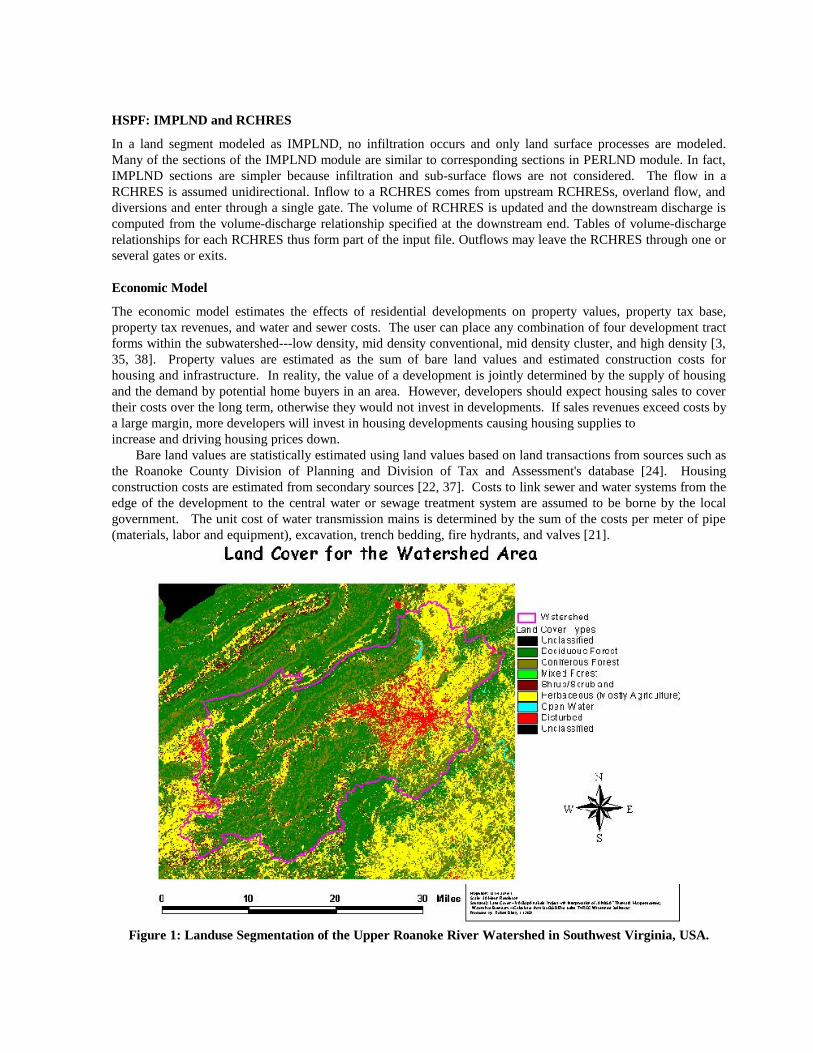
Figure 1: Landuse Segmentation of the Upper Roanoke River Watershed in Southwest Virginia, USA.

3 Experimental Studies

Example Scenario

An initial prototype of our system is available at the URL http://landscapes.ce.vt.edu and covers the 57 square-mile Back Creek subwatershed of the Upper Roanoke River watershed (Fig. 1) in Southwest Virginia, USA. Typically, the user invokes the thin-client Java applet (Fig. 2) depicting the Back Creek subwatershed and uses the cursor to specify landuse distributions for individual land segments. By selecting the “hydrology expert” interface (Fig. 3) over the “decision maker” interface in Fig. 2, hydrologists can use an HSPF input file that they have created, allowing more control when greater expertise is available. The cursor locations are converted and communicated via messages to a server, where each individual message contains details of the coordinates on the map (where clicked), parameters for running a simulation, or a command to indicate a particular simulation. Using MapObjects on the 600m^2 per pixel grid helps us provide map layer functions, automatic drawing of the map on the server, and transmission of maps across the internet. In particular, MapObjects provides primitives for intercepting coordinates of clicks on the map in the applet. Based on the user input, L2W calculates the new distribution of landuses, suitable for input to HSPF, which is then run on one “base” rainfall pattern for a pre-selected duration. HSPF Model Parameters and Calibration

The HSPF model requires input data on rainfall, stream flow, evaporation, soil, and landuse information. Hourly records of rainfall data were obtained from the Blacksburg office of the National Weather Service. Flow data for Dundee stream gage on Back Creek were obtained from the USGS office in Richmond, VA. Potential evapotranspiration values were calculated on a monthly basis using the Thornthwaite method [40]. Physical watershed data were obtained from USGS 30-meter DEMS, USGS stream reach overlays, and Virginia Gap landuse data. Landuse data were classified into the following categories: Forest, Herbaceous/Agriculture, Disturbed, Mixed, and impervious land. Reach cross-section data were collected in a field visit and from the Roanoke Valley Regional Stormwater Management Plan [14]. Based on the distribution of landuse and stream reaches, the watershed was divided into ten segments drained by ten stream reaches.

HSPF is a heavily parameterized model and uses both conceptual and physical parameters to represent hydrologic processes occurring within a watershed. Some physical parameters include land slope, overland flow plane length, Manning's roughness coefficient, infiltration rate of soil, and interception capacities of the vegetation. The conceptual parameters include storage capacities in the upper and lower zones of the soil, groundwater recession flow parameter, and evapotranspiration rates from various storages. The initial estimate of parameters was made based on published studies including the Upper James River study, conducted as a part of the EPA's Chesapeake Bay model [15]. In general, parameters associated with the upper soil zone varied with landuse, while the watershed slope varied among the ten physical land segments. Forest, herbaceous/agriculture, mixed, and disturbed lands were modeled as PERLND segments while impervious land was represented as an IMPLND segment.

The model was calibrated for water years 1995, 1996, and 1997 using the USGS/EPA HSPEXP expert system shell. Calibration consisted of matching simulated and observed results for annual flow volume, high and low flow volumes, storm peaks, and seasonal volume differences. Parameter changes were made by varying the parameter by a fixed percentage for all landuses in all areas, while maintaining the relative differences in parameters between landuses. Calibration was considered complete when expert system advice did not improve model performance. The performance of the calibrated model was validated on water year 1998 and incorporated into the PSE. Results of simulation runs taken with PSE version of HSPF for examining various `what if' scenarios were satisfactorily compared to the results of similar runs taken by running the model outside the PSE.

Figure 2: Front-End Decision Maker Interface to the L2W PSE.

Figure 3: Front-End Hydrology Expert Interface to the L2W PSE.

Economic Model Calibration A total of 1,844 transactions of vacant and nonvacant land parcels for the period of 1996 to 1997 were used to estimate bare land values, which equal the value of the parcel minus the value of structures on the land. The assessed values of structures located on parcels were deducted from the parcel transaction prices - a procedure used by Bockstael and Bell [7]. Estimation was performed using traditional linear least squares approximations. Further work is being done to evaluate alternative statistical procedures. The resulting estimated model is

log(Price) = -17.87 - 0.53[log(Size)] -0.02{[log(Size)]}2 + 0.41[log(Elevation)] - 0.13{[log(Elevation)]}2 - 0.05(Soil1) -0.10(Soil2) + 0.0037(Population) -0.0005{(Population)}2 + 1.60[log(Mall)] -0.25{[log(Mall)]}2 + 2.47{log[log(City)]} + 0.13(Developed) - 0.07(Road) + 0.05(Year) + 4.09[log(X)] + 3.72[log(Y)] - 0.91[log(X)log(Y)]

where Price is the price of the parcel per square meter, Size is the area of the parcel in square meters, Elevation is the average elevation of the parcel in meters, Soil1 and Soil2 are dummy variables for soil permeability with Soil1 being least permeable and Soil2 intermediate in permeability, Population is the population density (persons/hectare) in the U.S. Census block containing the parcel, Mall is the minimum distance to an existing mall, City is the minimum distance to the closest city (Roanoke or Blacksburg depending on parcel location), Developed indicates whether the parcel is vacant or contains a commercial or a residential structure, Road reveals whether the parcel is adjacent to a major road, the variable Year shows if the parcel was sold in 1996 or 1997, and the coordinates X and Y determine the exact location of the parcel [24].

Figure 4: Land Segments in the Back Creek Subwatershed.

Rationale for Tract Placements The main rationale for selecting tract sites for the example runoff scenario is based on the determination of developability within the watershed. The concept of developability for a particular tract site is derived from a raster overlay of four spatial data layers---slope, landuse, preservation status, and flood plain location. In the overlay, the pixels in each of the four layers are reclassified with a value of either 0 or 1. The value assigned depends on whether the original value meets the criteria for developability. For example, pixels with average slopes of less than 20% are developable and are assigned a 0, while those over 20% are not developable and are assigned a 1. Each of the other layers is reclassified in a similar method (Table 2). If any one of the four layers for a pixel is equal to one, then the pixel is not developable. Overall developability for a particular pixel, therefore, is achieved by summing the values for each of the four layers. If they sum to zero, then the pixel is developable; if the sum exceeds zero, then it is not developable. Within Back Creek subwatershed, land segments 3, 4, 5, and 10 (Fig. 3) have significant portions of developable lands. These land segments, therefore, provide prime sites for adding new development tracts. The larger problem of misclassified and unlabeled data caused by out-of-date field measurements and lack of knowledge of precise commercial and vegetation boundaries is endemic to this domain; in the future, we plan to make use of machine learning techniques [8] to aid in automatic landuse segmentation. This is related to the broader task of map analysis using GIS data, a problem that has received much attention in areas such as identifying clusters of wild life behavior in forests [4], modeling population dynamics in ecosystems [1], and socioeconomic modeling [5].

GIS Layer Criteria Value

Slope

>20% <20%

1 0

Landuse

Distrubuted and Water Forest and Herb/Agr

1 0

Preservation Status

Preserved Unpreserved

1 0

Flood Plain Location Inside Flood Plain Outside

1 0

Raster Overlay Sum of Values 0 = Developable >0 = Developable

Table 2: Method of Raster Overlay for Determining Developability.

Interaction Scenario

The prototype allows the user to specify: (1) changes to the land segments in terms of settlement patterns (for example, “add 1000 people in a settlement pattern equivalent to Preston Forest”) and (2) a choice of simulating several predetermined rainfall scenarios (`dry summer,' `wet summer,' `fall with a hurricane'). The hydrologic simulation results include comparison of annual runoff (in inches), and selected storm peaks with a baseline scenario, and can be viewed at subwatershed scale as well as at the outlet of the watershed. Once this is complete, users will be able to analyze effects of various possible land settlement scenarios in a way that is meaningful to a city planner, economist, or hydrologist. The L2W prototype provides hydrographs (continuous record of streamflow at selected points) and relevant tabular statistics of annual runoff in inches, changes in storm peaks, and statistics of low flow. Figs. 2 and 3 present the input interfaces to our system and Fig. 5 identifies sample outputs obtained from an evaluation. Note that Fig. 5 provides comparisons between the effects of the alternative landscape scenario with a baseline case. In turn, these are useful in making biological impact assessments (on aquatic conditions), changes in flood risk, and land price changes.

Interpretation of Hydrological Results from Example Scenario

The PSE produces average daily flow results for each of the ten land segments (Fig. 5). The land segments run downstream from 1 to 10, with 10 being the outlet for Back Creek. Land segments 1 and 2 show no change in average daily flows as a result of the new tracts in the watershed. This result is intuitive because all of the tracts are downstream of these two land segments. The three tracts placed in land segment 3 are low density residential (few impervious surfaces) and, therefore, have very little impact on the hydrograph. Land segments 4 and 5

contain considerably more tracts with more impervious surfaces. This arrangement results in increased average daily flows and runoff. Increased flows and runoff continue to exist in land segments 6 through 9 as the effects from upstream segments are carried downstream. Results from land segment 10 also show increased flow and runoff, but the effects are not that pronounced, considering the new development tracts added to the land segment. Perhaps this lack of effect is attributable to the larger overall stream size and baseline flow.

Figure 5: Graph output indicating runoff impact resulting from altering landuse values in Segment 5.

Interpretation of Results from Economic Model The economic model outputs are shown in Table 3 for a scenario of developing 50 housing units using low, mid, and high density forms for development tracts. Total land area and land devoted to housing lots, infrastructure, and open space are shown in the table. Estimated bare land values are based on average lot sizes devoted to housing as shown in the equation earlier. Low density shows the largest total value because it results in the most land developed. Land areas developed and total land values decline with mid density standard, mid density cluster, and high density, which have smaller lot sizes. Total development costs are also highest with low density, which has the largest total area to cover and the most expensive type of housing. Total tract value is also highest with low density and lowest with mid density cluster development.

Development Tract Form Low Density Mid Density Standard

Mid Density Cluster

High Density

Development Landuses

Land Reserved For Open Space (ha) 0.0 2.0 3.8 0.0 Land Occupied by Housing (ha) 55.8 5.6 4.1 4.0

Land Occupied by Infrastructure (ha) 4.9 0.9 0.6 0.9 Total Land (ha) 60.7 8.5 8.5 4.9

Total Number of Housing Units 50.0 50.0 50.0 50.0 Dollar Change Relative to Predevlopment Baseline

Bare Land Value $2,256,647 $1,118,137 $1,005,880 $1,001,845 Tract Development Cost $11,966,769 $8,513,661 $8,411,118 $8,420,094

Total Assessed Value $13,296,223 $9,210,933 $9,098,675 $9,098,194 Tax Revenue $150,247 $104,084 $102,815 $102,810

Cost to Local Government $0 $378,985 $378,985 $378,985 Annualized Cost to Localities $0 $30,546 $30,546 $30,546

Table 3: Estimated Tax Revenues and Fiscal Costs by Development Tract Form.

4 Concluding Remarks The long-term goal of our project is to provide a holistic approach to watershed management by an integrated assessment of the alternative landscape scenarios that occur during the urbanization/suburbanization process. On the PSE front, we plan to explore various additional aspects, as outlined in Table.~\ref{compare}. The operational strength of watershed management PSEs will increasingly rely on an integration of methodologies for storage, retrieval, and postprocessing of scenarios and experiments. The importance of support for such data intensive operations is increasingly underscored in scientific circles [10, 29, 30, 34]. One of the emerging areas in database research is to provide native support for domain specific analyses. This is the approach taken by the multi year, multi institution Sequoia earth science project [39]. In the L2W context, we plan to extend this methodology to provide storage for scenario populations in a structured way, and enable management of the execution environment (e.g., HSPF) by keeping track of constraints implied by the physical characteristics of the application. This will be achieved by a one-to-one correspondence between the entities in the scenario description to, say, tables in a relational database system (RDBMS). In addition, scenario evaluation can be efficiently formulated as query answering. For example, the SQL query SELECT RunOff(*) FROM Roanoke WHERE slope < 12 AND landuse = 'Preston Forest';

can be used to evaluate the runoff arising in subwatersheds that satisfy the desired conditions. Powerful query optimization algorithms have been developed [11, 20] that selectively `push' costly GIS operations into the computational pipeline. In addition, useful conceptual abstractions for reasoning about the watershed domain and supporting the problem solving process need to be developed. The ZOO desktop experiment management system [23] has taken the first steps towards this goal by providing a compositional modeling environment for data collection, pre-processing, and management of experiments. However, ZOO lacks decision support capabilities and will require fairly detailed domain modeling before application to watershed management. The connections to GIS based services also need to be strengthened in PSE design methodology. Wildlife and fisheries biologists were involved in the L2W project, but their data and models were not completed as of this writing. The intent of L2W is to integrate hydrologic, economic, and biological models. Finally, we intend to explore the incorporation of collaboration support, optimization, and recommender systems (for selecting among various choices of simulation models) within the L2W framework.

References [1] C.A. Abbott, M.W. Berry, J. Comiskey, L.J. Gross, and H.=K. Luh. Parallel Individual-Based Modeling of

Everglades Deer Ecology. IEEE Computational Science and Engineering, Vol. 4(4), October-December, 1997.

[2] J. Andrew, J. Capilla, and E. Sanchis. AQUATOOL, A Generalized Decision-Support System for Water-

Resources Planning and Operational Management. Journal of Hydrology, Vol. 177:pp. 269-291, 1996. [3] R. Arendt. Designing Open Space Dubdivisions: A Practical Step-by-Step Approach. Natural Lands Trust,

Media, PA., 1994. 96 pages. [4] M.W. Berry, J. Comiskey, and K. Minser. Parallel Analysis of Clusters in Landscape Ecology. IEEE

Computational Science and Engineering, Vol. 1(2):pp. 24-38, Summer 1994. [5] M.W. Berry, R.O. Flamm, B.C. Hazen, and R.L. MacIntyre. The Land-Use Change Analysis System

(LUCAS) for Evaluating Landscape Management Decisions. IEEE Computational Science and Engineering, Vol. 3(1):pp. 24-25, 1996.

[6] B.R. Bicknell, J.C. Imhoff, J.L. Kittle, A.S. Donigan Jr., and R.C. Johnson. Hydrological Simulation

Program – FORTRAN (HSPF). User’s Manual for Version 11.0. Technical report, National Exposure Research Laboratory, Research Triangle Park, US EPA, NC 27711, USA, August 1997.

[7] N.E. Bockstael and K. Bell. Land Use Patterns and Water Quality: The Effect of Differential Land

Management Controls. Kluwer Academic Publishers, Boston, 1998. [8] C.E. Brodley and M.A. Friedl. Identifying Mislabeled Training Data. Journal of Artificial Intelligence

Research, Vol. 11:pp. 131-167, 1999. [9] S. Carpenter, W. Brock, and P. Hanson. Ecological and Social Dynamics in Simple Models of Ecosystem

Management. Conservation Ecology, Vol. 3(2), 1999. [10] K.M. Chandy, R. Bramley, B.W. Char, and J.V.W. Reynders. Report of the NSF Workshop on Problem

Solving Environments and Scientific IDEs for Knowledge, Information and Computing (SIDEKIC’98). Technical report, Los Alamos National Laboratory, 1998.

[11] S. Chaudhuri and K. Shim. Optimization of Queries with User-Defined Predicates. ACM Transactions on

Database Systems, Vol. 24(2):pp. 177-228, June 1999

[12] C.W. Chen, J. Herr, L. Ziemelis, R.A. Goldstein, and L. Olmsted. Decision Support System for Total Maximum Daily Load. Journal of Environmental Engineering, Col. 125(7):pp. 653-659, 1999

[13] N.H. Crawford and R.K. Linsley. Digital Sumulation in Hydrology: Stanford Watershed Movel IV.

Technical Report 39, Department of Civil Engineering, Stanford University, July 1966. [14] Dewberry and Davis. Roanoke Valley Regional Stormwater Management Plan, Study Report. Fifth

Planning District Commission, Roanoke, VA, December 1996. [15] A.S. Donigan Jr., B.R. Bicknell, and J.L. Kittle Jr. Conversion of the Chesapeake Bay Basin Model to HSPF

Operation. Prepared by AQUA TERRA Consultants for the Computer Sciences Corporation, Annapolis, MD and U.S. EPA Chesapeake Bay Program, Annapolis, MD, 1986.

[16] A.S.. Donigan Jr., J.C. Imhoff, and J.L. Kittle Jr. HSPFParm, An Interactive Database of HSPF Model

Parameters Version 1.0. AQU TERRA Consultants, CA, 94043, 1999 [17] K. Fedra GIS and Environmental Modeling. In M. Goodchild, B. Parks, and L. Steyaert, editors,

Environmental Modeling with GIS, pages 35-50. Oxford University Press, 1993. [18] K. Fedra and D.G. Jamieson. The Waterware Decision Support System for River-Basin Planning: 3.

Example Applications. Journal of Hydrology, Vol. 177:pp. 199-211, 1996 [19] M.F. Goodchild. The State of GIS for Environmental Problem-Solving. In M. GoodChild, B. Parks, and L.

Steyaert, editors, Environmental Modeling with GIS, pages 8-15. Oxford University Press, 1993. [20] J.M. Hellerstein. Optimization Techniques for Queries with Expensive Methods. ACM Transactions on

Database Systems, Vol. 23(2):pp. 113-157, September 1998. [21] R.S. Means Company Inc. Residential Cost Data 1999. Kingston, MA, 1999. [22] R.S. Means Company Inc. Site Work and Landscape Cost Data 1999: 18th Annual Edition. Kingston, MA,

1999. [23] Y, Ioannidis, M. Livny, S. Gupta, and N. Ponnekanti. ZOO: A Desktop Experiment Management

Environment. In Proc. 22nd International VLDB Conference, pages 274-285, 1996. [24] I.K. Katsas and D.J. Bosch. Land Value Modeling in Roanoke County. Unpublished Manuscript,

Department of Agricultural and Applied Economics, Virginia Tech, Blacksburg, VA, April 2000. [25] J.L. Kittle Jr., A.M. Lumb, P.R. Hummel, P.B. Duda, and M.H. Gray. A Tool for the Generation and

Analysis of Model Simulation Scenarios for Watersheds (GenScn). Technical Report 98-4134, U.S. Geological Survey Water-resources Investigations, 1998. 152 pages.

[26] R.G. Knox, V.L. Kalb, E.R. Levine, and D.J. Kendig. A Problem-Solving Workbench for Interactive

Sumulation of Ecosystems. IEEE Computational Science and Engineering, Vol. 4(2):pp. 52-60, 1997/ [27] H. Lal, C. Fonyo, B. Negahban, J.W. Jones, W.B. Boggess, G.A. Kiker, and K.L. Campbell. Lake

Okeechobee Agricultural Decision Support System (LOADSS). ASAE Paper No. 91-2623, American Society of Agricultural Engineers, St. Joseph, Michigan, 1991.

[28] D.R. Maidment. GIS and Hydrological Modeling. In M. Goodchild, B. Parks, and L. Steyaert, editors,

Environmental Modeling with GIS, pages 147-167. Oxford University Press, 1993.

[29] R.W. Moore, C. Baru, R. Marciano, A. Rajasekar, and M. Wan. Data-Intensive Computimg. In C. Kesselman and I. Foster, editors, The Grid: Blueprint for a New Computing Infrastructore. Morgan Kaufmann, 1998.

[30] R.W. Moore, T.A. Prince, and M. Ellisman. Data-intensive Computing and Digital Libraries.

Communications of the ACM, Vol. 41(11):pp. 56-62, November, 1998. [31] Negahban, B. and Moss, C.B. and Jones, J.W. and Zhang, J. and Boggess, W.D and Campbell, K.L.

Optimal Field Measurement for Regional Water Quality Planning. ASAE Paper No. 94-353, American Society of Agricultural Engineers, St. Joseph, Michigan, 1994.

[32] D.L. Osmond, R.W. Gannon, J.A. Gale, D.E. Line, C.B. Knott, K.A. Phillips, M.H. Turner, M.A. Foster,

D.E. Lehning, S.W. Coffey, and J. Spooner. WATERSHEDSS: A Decision Support System for Watershed Scale NonPoint Source Water Quality Problems. Journal of the American Water Resources Association, Vol. 33(2):pp. 327-341, 1997.

[33] J.R. Philip. The Theory of Infiltration. Soil Science, Vol. 84:pp. 257-264, 1957. [34] J.R. Rice and R.F. Boisvert. From Scientific Software Libraries to Problem-Solving Environments. IEEE

Computational Science & Engineering, Vol. 3(3):pp. 44-53, Fall 1996. [35] T. Schuler et al. The Benefits of Better Site Design in Residential Subdivisions. Watershed Protection

Techniques, Col. 3(2):pp. 633-646, 2000. [36] M. Shapiro et al. GRASS Version 4.1 Programmer’s Manual. Technical report, U.S. Army Corp. of

Engineers’ Construction Engineering Research Laboratory, Champaign, IL, March 1994 [37] C. Speir. Two Cost Analyses in Resource Economics: The Public Service Costs of Alternative Land

Settlement Patterns and Effluent Allowance Trading in Long Island Sound. Unpublished M.S. Thesis, Virginia Tech, Blacksburg, VA, 2000.

[38] K. Stephenson. Proposed Development Tracts for Development Scenarios. Unpublished Manuscript,

Department of Agricultural and Applied Economics, Virginia Tech, Blacksburg, VA, 2000. [39] M. Stonebraker. Sequoia 2000: A reflection on the First Three Years. IEEE Computational Science and

Engineering, pages 63-72, Winter 1994. [40] C.W. Thornthwaite. An Approach Toward a Rational Classification of Climate. Geograph. Rev., Vol.

38:pp. 55-94, 1948. [41] USEPA. Better Assessment Science Integrating Point and Nonpoint Sources – Users Manual, Version 1.0.

Technical Report EPA-823-R-96-001, Environmental Protection Agency, District Court, Washington, DC, 1966.