fresco: coupled-channels calculations · lawrence livermore national laboratory llnl-pres-667633 3...

LLNL-PRES-667633 This work was performed under the auspices of the U.S. Department of Energy by Lawrence Livermore National Laboratory under Contract DE-AC52-07NA27344. Lawrence Livermore National Security, LLC

FRESCO: Coupled-channels Calculations Finite-Range with Exact Strong COuplings.

Talk at INT 15-58W, Seattle

Ian Thompson

Wed, March 4, 2015

Lawrence Livermore National Laboratory LLNL-PRES-667633

2

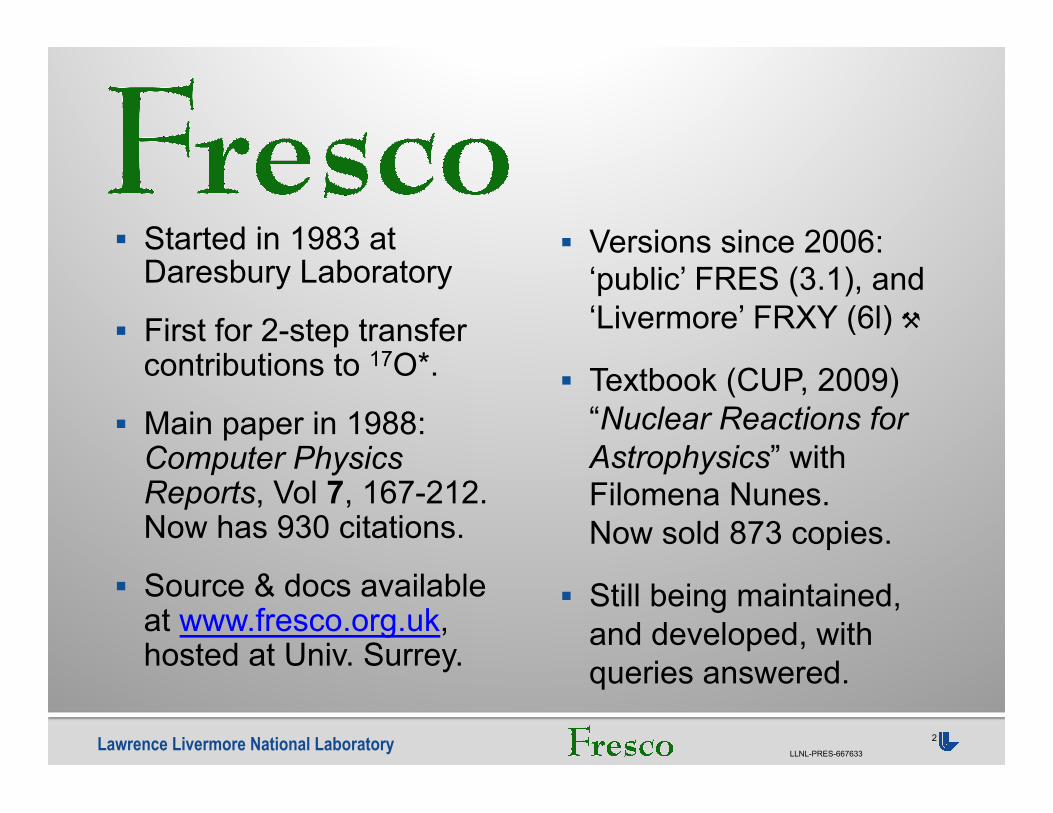
§  Started in 1983 at Daresbury Laboratory

§  First for 2-step transfer contributions to 17O*.

§  Main paper in 1988: Computer Physics Reports, Vol 7, 167-212. Now has 930 citations.

§  Source & docs available at www.fresco.org.uk, hosted at Univ. Surrey.

§  Versions since 2006: ‘public’ FRES (3.1), and ‘Livermore’ FRXY (6l)

§  Textbook (CUP, 2009) “Nuclear Reactions for Astrophysics” with Filomena Nunes. Now sold 873 copies.

§  Still being maintained, and developed, with queries answered.


3

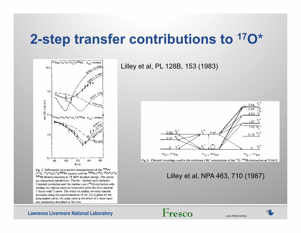
2-step transfer contributions to 17O*

Lilley et al, NPA 463, 710 (1987)

J.S. Lilley et al. / Multistep effects 719

where H~ -) and H~ +) are Coulomb functions with incoming and outgoing boundary conditions.

(4.3) Er.p-r = E + QK -- ep-- e T

for excited state energies ep, e T and Q-value QK in partition K and

2mK E ] 1/2 K o = , (4 .4)

where mK is the reduced mass in the channel with partition K. The U K ( R K ) are diagonal optical potentials, vr~,(RK) the local inelastic form factors of multipolarity F, and V ~ , ( R K , RK,) are the transfer form factors. The inclusion of non-orthogonality terms modifies these equations as is described in ref. 20).

The iterative solution of the coupled equations proceeds by regarding the right- hand sides as source terms that are approximated by using the wave functions from the previous iteration. The first iteration therefore ignores these terms, and hence is just an elastic scattering calculation. The second iteration uses the source term with only the elastic channel ao to be non-zero, and hence is equivalent to a first-order DWBA calculation. Subsequent iterations are equivalent to higher-order Born approximations, and continue until the S-matrix elements settle to a prescribed accuracy. Absolute accuracy criteria are used, to avoid spending too long settling the details of weak channels. Sometimes the iterations diverge, for example, when near resonances and this necessitates using Pad6 acceleration of the S-matrix elements. This is equivalent to allowing explicitly for the complex poles which describe the resonances.

The spins and energies of the excited states in the 160, 170 and 180 partitions are shown in fig. 6 (certain states are not included as FRESCO is limited to a transferred angular momentum less than 7). The present calculations used a matching radius, Rm = 50 fm, and included partial waves up to L = 300. The 170 nucleus was treated as an 160 core plus a neutron in either the 0d5/2 or lsl/2 single-particle state. Hence,

2.54 3/2+ 2.49 7/2+ 2.03 1/2+

1.57 ~'2

1.42 15/2- 0.90 ~2"- _. 1/2 + 0.87 0.78 1'/2+

I 1/-- J ~ 5/;+ 0 9+ 0 2 C - - - ~ 2 0 72

18 0 + 207pb 17 0 + 2°8pb 16 0 + 209pb

Fig. 6. Channel couplings used in the multistep CRC calculations of the 170-2°8pb interaction at 78 MeV.

Lilley et al, PL 128B, 153 (1983)

Volume 128B, number 3,4 PHYSICS LETTERS 25 August 1983

10.0

1.0

"C"

..Q E

C e 0.1

1.0

0.1

208pb(';'O,170,'~II/2~'II~'OSpb Elab=78 MeV

/ /

\ " ,,_,/ /

;eOapb( '80.180*(21+))2°apb E~ab = 78

L 8'o 18o

0c.m.

Fig. 2. Differential cross section measurements of the 2°8Pb (170, 170*(1/2+))208pb (upper) and the 2°8pb (lSo, 180*(2+)) 208pb 0ower) reactions at 78 MeV incident energy. The curves are theoretical calculations. The dot-dashed curve includes Coulomb excitation and the nuclear core (160) excitation only. Adding the valence neutron interaction gives the short-dashed ("direct only") curve. The effect of adding two-step transfer processes using the approximations of ref. [ 1 ] is given by the long-dashed curve; the solid curve is the result of a more rigor- ous calculation described in the text.

ancy in this region would be difficult to reconcile since the forward-angle cross sections are determined mainly by the Coulomb amplitude, which is well known. The do t -dash curve is calculated for the core contribution only (which includes Coulomb excitation) and is an inadequate fit at all but the most forward angles. The short-dashed curve (direct) includes both the real and imaginary contributions of the valence neutrons as well as the core. The imaginary part of the valence form factor is comparable with that of the real part, and the data show that both must be included to achieve what is a much bette r representation of the reaction. The im-

portance of the imaginary valence term was emphasised by the authors of ref. [1].

Adding the contribution of the two-step transfer mechanism gives the distribution shown by the longo dashed curve. In this 180 calculation, the two-step amplitudes have been corrected for the normalisation error noted at the end of ref. [ 1 ]. The interference minimum now is reproduced both in position and depth, although there is some indication experimentally that the minimum is a little sharper than predicted. The yield at larger angles suggests that there may be a somewhat larger two-step component than was calculated, although this is by no means conclusive. Increas- ing the two-step contribution might improve the fit at back angles. On the other hand, it would decrease the forward angle cross sections and shift the interference minimum, all of which could result in a worse overall fit.

Further work is planned to extend the data to larger angles in the hope that this will help to distinguish between effects of a stronger nuclear inelastic amplitude and details of the elastic scattering interaction. It should be remembered that the theoretical calculations shown here are in no way a fit to the present data, having been published before the measurements were taken. The overall agreement with experiment is very good indeed, and supports the conclusion of ref. [ 1 ] that the two-step amplitudes are not important for this particular reaction.

The situation is quite different for the inelastic excitation of the 170 projectile. These data show a marked deviation from the direct prediction support- ing the expectation of the authors of ref. [ 1 ] that two- step effects should be important if not dominant in this example. The original prediction, including two-step effects, is shown as the long-dashed curve. It was noted in ref. [1] that these calculations contain certain approximations which could alter them significantly. In- deed, the data are not well represented by this curve.

New calculations of the two-step amplitudes have been carried out which overcome many of the draw- backs of the previous ones. They are made in full finite range and take proper account of recoil and non- orthogonality effects. The result of these latest calculations is shown as the solid curve in the figure, and is in much better agreement with the measurements.

The transfer calculations were performed with the code FRESCO [4]. This code is designed to solve

155


4

§  Methods of Direct Reaction Theories, paper in “Scattering” ed. Pike & Sabatier (2001)

§  User Guide: Appendix A of Nuclear Reactions for Astrophysics(2009)

§  Coupled Channels Methods for Nuclear Physics, (1988)

§  Input manual See http://www.fresco.org.uk/documentation.htm

Documentation


5

Basic Idea §  Reactions between two

nuclei: entrance and exit

§  Multiple mass partitions.

§  Energy, spin and parity given for all initial and final states of all nuclei.

§  Unlimited lists of potentials and couplings.

§  Solve coupled equations

§  Predict cm cross section distributions.

§  Standard forms for •  optical potentials, •  bound states, •  inelastic, transfer and

capture mechanisms, •  etc

§  Written in Fortran 90 •  Tested on wide range of

compilers


6

The Coupled Equations

102 Scattering theory

wave functions with some part of the Hamiltonian. These integral formsfor the S- or T-matrix elements should in principle yield identical results,but are useful since they may suggest a new range of approximations thatmay still be sufficiently accurate in the relevant physical respects.

3.3.1 Green’s function methodsUp to now we have solved only homogeneous Schrodinger equations like[E H] = 0. Sometimes we may need to solve inhomogeneous equa-tions like [E H] = with outgoing boundary conditions, for someradial functions (R) called source terms, as such equations arise as partof a coupled-channels set. The inhomogenous equation may be solved bydifferential methods as discussed in Chapter 6, but often it is useful to givean integral expression for its solution, and it is especially useful that thereexist simple integrals giving directly the asymptotic outgoing amplitude ofthe solution, namely its T-matrix element. This section shows how to useGreen’s function methods to solve the inhomogeneous differential equa-tion.

Integral solutions of inhomogeneous equations

Consider the general problem of solving the coupled equations similar tothose of Eq. (3.2.52):

[TxL(R) + Vc(R) Expt] ↵(R) +X

↵0

h↵|V |↵0i ↵0(R0) = 0. (3.3.1)

for some given total angular momentum and parity Jtot and incoming chan-

nel ↵i that we assume are all fixed, and not always written among the in-dices. Here we have separated out the point-Coulomb potential Vc(R) =ZxpZxte2/R (if present), and put all the other couplings, local or non-local,into the matrix elements of V .

The solutions must satisfy the standard outgoing boundary conditionsof Eq. (3.2.13) for the given ↵i. Suppose that all the ↵0(R0) are knownfor which h↵|V |↵0

i 6= 0, in which case we may solve the inhomogeneousequation (3.3.1) for the wave function ↵(R) using the known source term

↵(R) =X

↵0

h↵|V |↵0i ↵0(R0). (3.3.2)

3.2 Multi-channel scattering 97

which gives a separate equation for each ↵0 combination of quantum num-bers. The set of all the equations for various ↵0 is called the set of coupledchannels equations.

The Hamiltonian and energy matrix element was abbreviated by h↵0|H

E|↵i = (HE)↵0↵. To evaluate all these, we note that

[H E]|↵i = [H E] |xpt : (LIp)Jp, It;Jtoti

= [Tx + Hx + Vx E] |xpt : (LIp)Jp, It;Jtoti

= [Tx + xp + xp + Vx E] |xpt : (LIp)Jp, It;Jtoti

= [Tx + Vx Expt] |xpt : (LIp)Jp, It;Jtoti, (3.2.45)

where Expt = E xp xp is the external kinetic energy for a givenexcited-state pair xpt.

This means that the matrix elements h↵0|H E|↵i may be written in

two ways, one by replacing H either by Tx + Hx + Vx for acting on theright hand side, and the other by Tx0 + Hx0 + Vx0 for acting on the leftside. The first option is called the prior form of the matrix element, andthe second the post form. Ideally, if all terms of the coupled equations areincluded and the equations are solved accurately, both choices will give thesame results.18 The prior form of the matrix element is thus

(HE)↵0↵ = Rx0h↵0

|Tx + Vx Expt|↵iR1x

= Rx0h↵0

|↵iR1x [TxL Expt] + Rx0

h↵0|Vx|↵iR

1x

N↵0↵[TxL(Rx) Expt] + V prior↵0↵ , (3.2.46)

where the partial-wave kinetic energy operator, the same as the one-channeloperator of Eq. (3.1.10), is

TxL(Rx) =

~2

2µx

d2

dR2x

Lx(Lx+1)R2

x

, (3.2.47)

where Lx is the orbital angular momentum in channel ↵. The couplinginteractions between channels are either the prior or post matrix elementsdefined as

V prior↵0↵ = Rx0

h↵0|Vx|↵iR

1x (3.2.48)

V post↵0↵ = Rx0

h↵0|Vx0

|↵iR1x (3.2.49)

18 On page 115 we will see that there is also a simpler first-order result, whereby that post and priorforms necessarily give the same first-order transition amplitudes.

with

satisfying the boundary conditions


Rn:

Jtot

↵↵

i

(Rx) =i2

hH

Li

(↵, k↵Rx) ↵↵i

H+L (↵, k↵Rx) SJ

tot

↵↵

i

i.(3.2.10)

The S matrix SJtot

↵↵

i

gives the amplitude of an outgoing wave in channel↵ that arises from a incoming plane wave in channel ↵i, in addition to thescattering from a diagonal point-Coulomb potential. For all the non-elasticchannels ↵ 6= ↵i we have

Jtot

↵↵

i

(Rx) ↵ 6=↵i= H+

L (↵, k↵Rx)12i

SJtot

↵↵

i

, (3.2.11)

which is to be proportional to a purely outgoing wave. When ↵ = ↵i,Eq. (3.2.10) leads to a matching equation similar to Eq. (3.1.37) for theelastic channel.

The cross sections, we saw in subsection 2.4.4, depend on the channelvelocity13 multiplying the square modulus of an amplitude. It is thereforeconvenient to combine these velocity factors with the S matrix, by defining(for each Jtot)

S↵↵i

=r

v↵

v↵i

S↵↵i

(3.2.12)

where the velocities satisfy µ↵v↵ = ~k↵. The combination S matrix S↵↵i

may now be used to find the multi-channel cross sections, and its ma-trix elements may be more directly found from the boundary conditionsof Eq. (3.2.10) expressed as

Jtot

↵↵

i

(Rx) =i2

H

Li

(↵, k↵Rx) ↵↵i

H+L (↵, k↵Rx)

rv↵

i

v↵S

Jtot

↵↵

i

.

(3.2.13)Both S↵↵

i

and S↵↵i

can be regarded as complex numbers in matrices Sand S. The second (column) index in these matrices refers to the incomingchannel, and the first (row) index names the exit channel.

We can also define a partial-wave T matrix by S = I + 2iT where I isthe identity matrix,14 or

S↵↵i

= ↵↵i

+ 2iT↵↵i

(3.2.14)S↵↵

i

= ↵↵i

+ 2iT↵↵i

, (3.2.15)13 Strictly a speed, but this is the most common terminology.14 We will often write S = 1 + 2iT for simplicity.


wave functions with some part of the Hamiltonian. These integral formsfor the S- or T-matrix elements should in principle yield identical results,but are useful since they may suggest a new range of approximations thatmay still be sufficiently accurate in the relevant physical respects.

3.3.1 Green’s function methodsUp to now we have solved only homogeneous Schrodinger equations like[E H] = 0. Sometimes we may need to solve inhomogeneous equa-tions like [E H] = with outgoing boundary conditions, for someradial functions (R) called source terms, as such equations arise as partof a coupled-channels set. The inhomogenous equation may be solved bydifferential methods as discussed in Chapter 6, but often it is useful to givean integral expression for its solution, and it is especially useful that thereexist simple integrals giving directly the asymptotic outgoing amplitude ofthe solution, namely its T-matrix element. This section shows how to useGreen’s function methods to solve the inhomogeneous differential equa-tion.

Integral solutions of inhomogeneous equations

Consider the general problem of solving the coupled equations similar tothose of Eq. (3.2.52):

[TxL(R) + Vc(R) Expt] ↵(R) +X

↵0

h↵|V |↵0i ↵0(R0) = 0. (3.3.1)

for some given total angular momentum and parity Jtot and incoming chan-

nel ↵i that we assume are all fixed, and not always written among the in-dices. Here we have separated out the point-Coulomb potential Vc(R) =ZxpZxte2/R (if present), and put all the other couplings, local or non-local,into the matrix elements of V .

The solutions must satisfy the standard outgoing boundary conditionsof Eq. (3.2.13) for the given ↵i. Suppose that all the ↵0(R0) are knownfor which h↵|V |↵0

i 6= 0, in which case we may solve the inhomogeneousequation (3.3.1) for the wave function ↵(R) using the known source term

↵(R) =X

↵0

h↵|V |↵0i ↵0(R0). (3.3.2)

and

either local R=R´, or non-local R≠R´

For each total spin Jtot and parity π


7

Optical and Binding Potentials §  Central, spin-orbit

and tensor forces.

§  WS, Gaussian (etc) shapes, or read in.

§  Deformation by rotational model, or by arbitrary strengths

§  Linear energy interpolations.

 L-, J-, and parity-dependent potentials.

 Effective masses m*(r)

 Lane isospin couplings


8

Coupling Mechanisms §  Inelastic

•  Deformed optical potls. •  Single-particle excitations

§  Transfers of a cluster •  Zero range, LEA. •  Finite range •  Non-orthogonality terms.

§  Two-nucleon transfers •  From & to correlated 2N wfs

from correlated 1N wfs, or read in from 3-body code.

•  Sequential and Simultaneous

§  Capture to γ channels •  Ek in Siegert approx. •  Mk magnetic transitions —  (both in localized approx.)

§  R-matrix phenomenology

§  General LSJ couplings •  Local or non-local •  Numerical forms read in

  General partial wave couplings •  Numerical local or nonlocal


9

Solving the Coupled Equations §  Numerov integration of

equations with local couplings: ‘exact’

§  Iteration on non-local couplings (eg. transfers).

§  Use Pade acceleration if n-step DWBA diverges.

§  Use James Christley’s coupled-Coulomb wave functions CRCWFN for long-range multipoles

§  Isocentrifugal approx.

§  R-matrix solutions: •  Expand on eigenstates of

diagonal optical potls •  Need Buttle corrections. •  More stable numerically

  Lagrange-mesh method: •  From Daniel Baye (ULB) •  No Buttle correction needed

  MPI: to solve Jπ sets in parallel.

  OPENMP: to solve coupled equations for given Jπ.


10

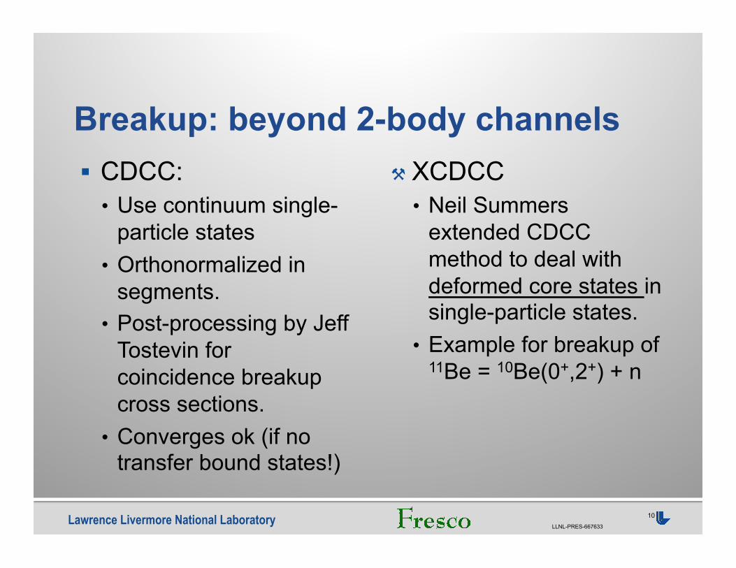
Breakup: beyond 2-body channels §  CDCC:

•  Use continuum single-particle states

•  Orthonormalized in segments.

•  Post-processing by Jeff Tostevin for coincidence breakup cross sections.

•  Converges ok (if no transfer bound states!)

 XCDCC •  Neil Summers

extended CDCC method to deal with deformed core states in single-particle states.

•  Example for breakup of 11Be = 10Be(0+,2+) + n


11

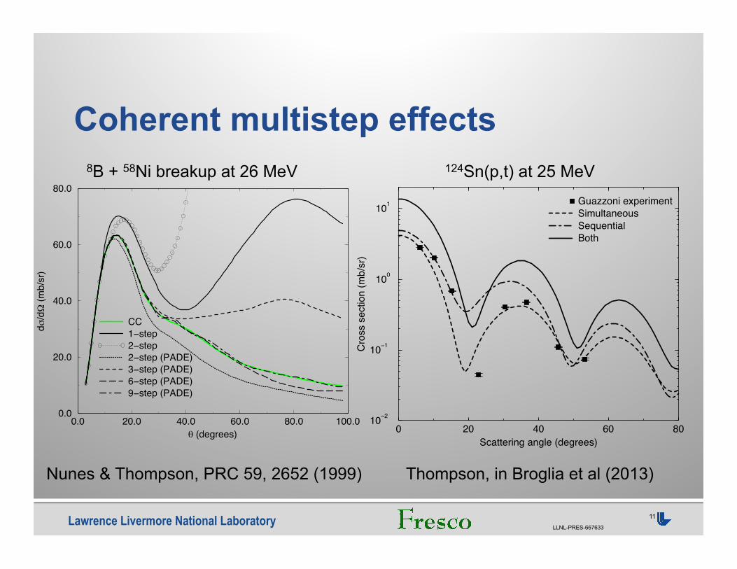
Coherent multistep effects

Nunes & Thompson, PRC 59, 2652 (1999)

0.0 20.0 40.0 60.0 80.0 100.0θ (degrees)

0.0

20.0

40.0

60.0

80.0

dσ/dΩ

(mb/

sr)

CC1−step2−step2−step (PADE)3−step (PADE)6−step (PADE)9−step (PADE)

8B + 58Ni breakup at 26 MeV 124Sn(p,t) at 25 MeV

0 20 40 60 80Scattering angle (degrees)

10−2

10−1

100

101

Cro

ss s

ectio

n (m

b/sr

)

Guazzoni experimentSimultaneousSequentialBoth

Thompson, in Broglia et al (2013)


12

Input Formats Output Formats §  OLD style #1:

•  Card inputs cols 1—72

§  NAMELIST style #2: •  Fortran var=value text

§  CDCC style #3: •  Generate easily the

NAMELIST sets of bins and couplings for CDCC calculations.

§  Cross sections σ(θ)

§  Amplitudes fmM:m’M’(θ)

§  CDCC amplitudes for post-processing.


13

Sfresco: searching for χ2 minimums §  Define data with errors:

•  Energy and/or angle data •  Polarization data •  Angle-integrated data •  Phase shifts in given channel •  Fitted bound state parameters

§  Define parameters Initial values and limits of: •  Optical parameters •  Spectroscopic amplitudes •  R-matrix pole energies & widths •  Data normalizations

§  Searching •  Interactive or given

method •  Uses MINUIT •  Plot initial or final fits •  Trace χ2 progress •  Restart at any trial set.


14

Current Developments   LLNL:

•  General nonlocal potentials •  Effective masses m*(R) •  Lane couplings for IARs •  IAR non-orthogonality (p,p′) •  Semi-direct capture step •  Surface operator for transfer

§  Jeff Tostevin: •  Breakup coincidence cross

sections with core excitation in XCDCC

•  Simple zero-range transfers

§  Alex Brown •  Using shell-model two-

nucleon overlaps for transfers (seq+sim).

§  Antonio Moro: •  Stabilizing the solutions

from Numerov method •  More NN standard forms for

tensor forces •  Deformations in optical

potentials in transfer operator


15

Missing Capabilities §  Core transitions in

electromagnetic particle steps.

§  Perey-Buck nonlocality in optical potentials.

§  Spin-dependence of optical potentials in transfer operators.

§  Energy-dependence of optical potentials in transfer operators.

§  Uniform treatment of antisymmetrization and identical particles

§  Convergence problems: CDCC breakup with all-order couplings to transfer channels.

fresco: coupled-channels calculations · lawrence livermore national laboratory llnl-pres-667633 3...

Documents