frequency domain analysis

1

Exercise 4.

Frequency Domain Analysis

Required knowledge

• Fourier-series and Fourier-transform.

• Measurement and interpretation of transfer function of linear systems.

• Calculation of transfer function of simple networks (first-order, high- and low-pass RC network).

Introduction

Signals are often represented in frequency domain by their spectrum, frequency, harmonic components, amplitude and phase. Time- and frequency-domain representations are mutually equivalent, and the Fourier transform can be used to transform signals between the two domains. Fourier transform exists for almost all practical signals which are used in electrical engineering practice. Frequency domain representation often simplifies the solution of several practical problems. It offers a compact and expressive form of signal representation by allowing the separation of spectral components. Frequency-domain representation can be effectively used in measurement of signal parameters, signal transmission, infocommunication, system design, etc.

One of the most important classes of signals is the class of periodic signals. Periodic signals are often used as excitation signals since they produce periodic signal with the same frequency at the output of the system the parameters of which are to be measured. Periodic signals are easy to observe with simple instruments like oscilloscopes, moreover averaging can also be effectively used to increase the signal-to-noise ratio. System parameters can be determined by measuring the amplitude gain (or attenuation) and phase shift between the output and input. Fourier transform allows the characterization of systems in a simple algebraic form instead of differential equations connected to time-domain representation.

Aim of the Measurement

During the measurement, the students study the method of signal analysis in frequency domain. They compare time domain algorithms to frequency domain ones. After finishing the measurement, they will be able to use frequency domain tools to describe properties of signals which are no trivial to be detected in time-domain. This laboratory lecture demonstrates how the students can apply their knowledge of signal and systems in order to solve engineering problems.

©BME-VIK Only students attending the courses of Laboratory 1 (BMEVIMIA304) are allowed to download this file, and to make one printed copy of this guide. Other persons are prohibited to use this guide without the authors' written permission.

Laboratory exercises 1.

2

Theoretical background

Fourier series and Fourier transform

Real-valued periodic signals can be decomposed into linear combination of sine and cosine functions. This trigonometrical series is referred to as Fourier series of signals, and it has the following form (T stands for the period, and T/2πω = denotes the angular frequency):

)sincos()(1

0 tkUtkUUtu Bk

k

Ak ω+ω+= ∑

∞

=

, (4-1)

where the coefficients can be calculated using the following equations:

∫=T

dttuT

U0

0 )(1, dttktu

TU

TAk ∫ ω=

0

)cos()(2, dttktu

TU

TBk )sin()(2

0∫ ω= . (4-2)

These operations are based on the orthogonality of trigonometric functions on the interval [0…T].

Fourier series have also a simpler form where complex-valued coefficients and complex exponential basis function are used:

∑∞

−∞=

ω=k

tjkCk eUtu 0)( , where ...2 ,1 ,0 ,)(1

0

±±== ∫ − kdtetuT

UT

tjkCk

ω (4-3)

For real-valued signals: )(conjugateC

kCk UU −= , i.e., Fourier components form complex

conjugate pairs.

The Fourier series of some practically important signals are summarized in the following table.

⎥⎦⎤

⎢⎣⎡ −ω+ω−ω

π= ...)5cos(

51)3cos(

31)cos(4)( tttAtx

⎪⎩

⎪⎨⎧

⎟⎠⎞

⎜⎝⎛ −= − oddisif1)1(4

evenisif02/)1( k

kA

kU kk

π

⎥⎦⎤

⎢⎣⎡ +++= ...)5sin(

51)3sin(

31)sin(4)( tttAtx ωωω

π

⎪⎩

⎪⎨⎧

= oddisif14evenisif0

kk

A

kU k

π

tT/2 T

A

t

x(t)

-T/4T/4

A x(t)


Exercise 4. Frequency Domain Analysis

3

⎥⎦⎤

⎢⎣⎡ +ω+ω+ω

π= ...)5cos(

51)3cos(

31)cos(8)( 22 tttAtx

⎪⎩

⎪⎨⎧

π= oddisif18

evenisif0

22 kk

A

kU k

⎥⎦⎤

⎢⎣⎡ −ω+ω−ω

π= ...)5sin(

51)3sin(

31)sin(8)( 22 tttAtx

⎪⎩

⎪⎨⎧

⎟⎠⎞

⎜⎝⎛ −

π= − oddisif1)1(8

evenisif0

22/)1(

2 kk

A

kU kk

Table 4-I. Fourier series of some periodic signals.

Fourier transform is the extension of Fourier series. It can be applied for square or absolute integrable functions. The spectrum of the signal x(t) is obtained using the Fourier transform as follows:

∫∞

∞−

−= dtetxjX tjωω )()( , (4-4)

The signal can be reconstructed from the spectrum X(jω) as follows:

∫∞

∞−

= ωωπ

ω dejXtx tj)(21)( . (4-5)

The Fourier transform of some important signals such as Dirac impulse, step function, sine and other periodic functions is not convergent in classical sense since they are not square integrable functions. However, the Fourier transform of such signals can also be interpreted using the Dirac delta function. The Fourier transform of a complex exponential function ejωt is a Dirac delta at the frequency of the signal, so the Fourier transform of general periodic signals can be easily expressed using the Fourier series (4-3):

∑∞

−∞=

±±=−=k

Ck kkUjX ...2 ,1 ,0)()( 0ωωδω , (4-6)

where ω0 denotes the fundamental frequency of the periodic signal, δ(ω–kω0) denotes the Dirac delta function at the frequency kω0. Dirac deltas are represented graphically as peaks at the frequencies where they are located. The spectrum (Fourier transform) of some typical periodic signals are illustrated in the following table.

tT T/2

A

t

x(t)

-T/4T/4

A x(t)



4

Spectrum of sine signal.

x(t)=A·cos(ω0t+φ)

The spectrum contains only two complex conjugate spectral components at frequency ±ω0.

Spectrum of a square signal.

Spectrum is decreasing with envelope 1/ω (dotted line). Only odd components (±ω0, ±3ω0, ±5ω0…) are present.

Spectrum of a triangle signal.

Spectrum is decreasing with envelope 1/ω2 (dotted line). Only odd components (±ω0, ±3ω0, ±5ω0…) are present.

Table 4-II. Fourier series of some periodic signals

It is important to note that it is not a general rule that the even harmonic components are missing from a periodic signal. For example, if the symmetry of a square wave differs from 50%, even spectral components will also appear.

Application of periodic signals as excitation signals

The most important excitation signals are sine wave and square wave. In some applications, (e.g., measurement of static nonlinear characteristics) triangular or saw tooth signals are also used.

Square wave is often used as excitation signal since it is easy to generate even with simple circuits, and it can be used to measure the step response of a system. When a square wave is applied as excitation signal, it is important that its half period should hold considerable longer (at least 5 or 10 times) than the largest time constant of the system to be investigated. In other words, the transient should vanish, and the steady state should be achieved before a new edge of the square wave. If this condition is fulfilled, the excitation signal can be regarded as a good approximation of a periodic step signal, so the response of the system can be regarded as its step response.

The shape of a signal in time domain allows us to make some important qualitative conclusions about its frequency-domain behavior. Since the square wave is not continuous (it contains steps at every level transition), so its spectrum is wide, i.e., it contains harmonic components of significant power in wide frequency range. It is an advantageous property when the square wave is used as excitation signal, since it excites the system in wide frequency range. Square wave is often used to test the frequency response of filters, amplifiers, etc. If the output of these systems is a clear square wave, then their transfer functions are frequency independent in a wide frequency range, so they cause small linear distortion on their input signals.

When an excitation signal is selected, both its time- and frequency-domain behavior should be considered. Some simple rules of thumb allow us to qualitatively determine the frequency-domain properties of a signal from its time-domain shape. The bandwidth of a signal is in close connection with its smoothness. The smoother a signal is, the faster its

ω0 -ω0

X(jω)

ω3ω0 -3ω0 5ω0-5ω0ω0 -ω0

X(jω)

ω3ω0-3ω0 5ω0-5ω0

ω0 -ω0

ϕjeA2

ϕjeA −

2

X(jω)

ω



5

Fourier coefficients (or amplitude spectrum) tend to zero, i.e., its bandwidth is small. The smoothness of a signal is characterized by its derivative functions. Generally, if the k-th derivative of a function is not continuous, then its amplitude spectra decreases

asymptotically as )1( +− kω . For example, the square wave is not continuous, i.e., k = 0, so

its spectrum decreases as ω1 . The spectrum of the triangular wave tends to zero faster than that of the square wave, since it is a continuous function, and its first derivative is not continuous (k = 1), so its spectrum decreases with envelope 21 ω . Intuitively speaking, high frequency spectral components are required to generate steep slopes and discontinuities in a function. E.g., a triangular wave is “smoother” than a square wave, so its bandwidth is lower if their frequencies are identical. It is worth to note, that if functions are approximated with finite Fourier sum, the error of the approximation is the highest in the vicinity of discontinuities (this phenomenon is called Gibbs-oscillation).

Measurement of the transfer function

It is well known that a linear time-invariant system can change only the phase and amplitude of a sine wave applied to its input. Hence, the system can be characterized at each frequency by a complex number (complex gain) whose phase is the phase shift of the system, and its magnitude is the gain of the system. The transfer function is the complex gain of the linear system as function of frequency.

Several methods are known which allow the measurement of the transfer function of linear systems. In the following, some of these methods are summarized (the emphasis is put on the measurement of magnitude characteristics).

Measurement of amplitude characteristics with stepped sine

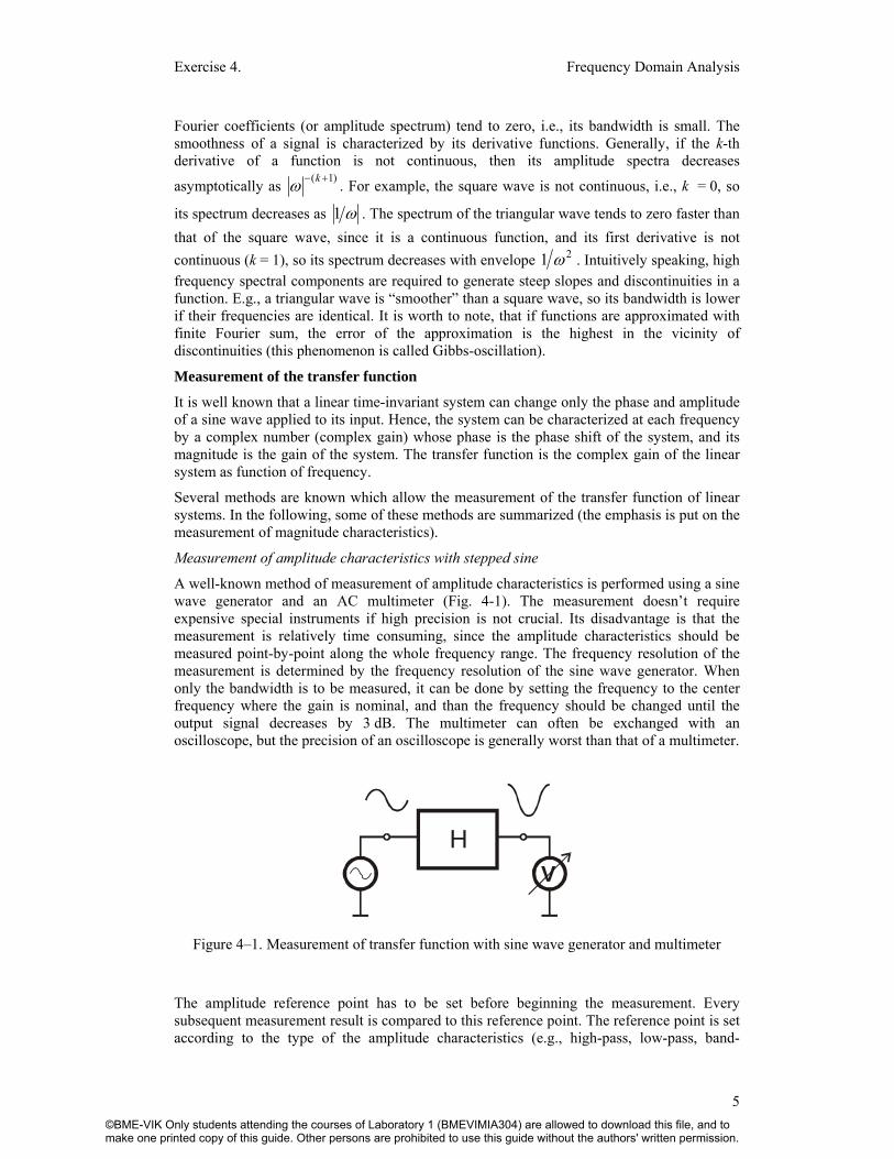
A well-known method of measurement of amplitude characteristics is performed using a sine wave generator and an AC multimeter (Fig. 4-1). The measurement doesn’t require expensive special instruments if high precision is not crucial. Its disadvantage is that the measurement is relatively time consuming, since the amplitude characteristics should be measured point-by-point along the whole frequency range. The frequency resolution of the measurement is determined by the frequency resolution of the sine wave generator. When only the bandwidth is to be measured, it can be done by setting the frequency to the center frequency where the gain is nominal, and than the frequency should be changed until the output signal decreases by 3 dB. The multimeter can often be exchanged with an oscilloscope, but the precision of an oscilloscope is generally worst than that of a multimeter.

HV

Figure 4–1. Measurement of transfer function with sine wave generator and multimeter

The amplitude reference point has to be set before beginning the measurement. Every subsequent measurement result is compared to this reference point. The reference point is set according to the type of the amplitude characteristics (e.g., high-pass, low-pass, band-



6

pass…). For example, if a system has low-pass characteristics as shown in Fig. 4–2, the reference point should be set at low frequency, at least one or two decades below the cutoff (corner) frequency. If the multimeter has fixed 0 dB point, it is recommended to set the input signal such that 0 dB appears at the output. Some of the modern multimeters allow us to set the 0 dB point to an arbitrary value. In this case, the input signal should be set as high as possible in order to ensure good signal-to-noise ratio. Care should be taken when setting the level of input signal! A common mistake is that the output signal becomes distorted, e.g., due to saturation, or the measured values are out of the range of the instruments. Except of some special cases, neither the input nor the output signals can exceed the supply voltage. If a passive circuit is measured (e.g., first-order RC network), no power supply is required. The level of input signal shouldn’t be changed during the whole measurement. It is generally recommended to check the shapes of the signals with an oscilloscope during the measurement.

⏐ ⏐[dB]H

log f

A

-20dB/dekád

-3 dB

1 10 100 1000

Figure 4–2. Transfer function of a low-pass filter

During the course of the measurement, the frequency is often changed logarithmically (see Fig 4–2), e.g., with steps 1-2-5-10-..., but it is recommended to measure with finer steps in the vicinity of the cutoff frequency. The cutoff frequency is often defined as the frequency where the amplitude characteristics decreases by 3 dB below the nominal value. (E.g., if the nominal gain is 9 dB, the gain is 6 dB at the cutoff frequency.)

The stepped sine wave method has the advantage that it offers a good signal-to-noise ratio. However, the measurement of the whole amplitude characteristics requires considerable time, since the frequency should be changed after each measurement, and we should wait until the transient vanishes after each time the frequency is changed.

Measurement of amplitude characteristics with multisine

In order to speed up the measurement, high bandwidth signals and frequency selective instruments (like spectrum analyzer or FFT analyzer) can be used to measure the whole amplitude characteristics in one step. Typical high-bandwidth excitation signals are multisine, swept sine (i.e., chirp), periodic sinc function, noise…

The multisine is a periodic excitation signal which consists of the sum of sine waves with different frequencies. The frequencies are generally integral multiples of a fundamental frequency. The amplitudes of the sine wave components can be set to an arbitrary level, however, it is practical to set the levels of the sine components to the same value. The phases of the components should be set to different values (often randomly) in order to ensure small crest factor (crest factor = peak value / RMS value). A given measurement setup limits the peak value of the excitation signal in order to avoid saturation, so if the crest factor is small,

20 dB/decade



7

the given peak value ensures high RMS value, i.e., good signal-to-noise ratio. Multisine signal will be generated by a function generator that can produce a preprogrammed multisine waveform.

1 256 512 768 1024-0.8 -0.6 -0.4 -0.2

0

0.2 0.4 0.6 0.8

1

time

ampl

itude

0 64 128 192 256 320 384 448 0

1

2

f requency

abs(

fft)

Figure 4–3. Multisine in time and frequency domain

The multisine is defined in time domain as follows:

( ) ( )∑=

+=F

kkkk tfAtx

12sin φπ , (4-6)

where F is the number of frequency components, and Tkfk = , where T is the period of the multisine.

Measurement of nonlinear distortion

Nonlinear distortion is caused by systems whose output is not a linear function of their inputs. If this static nonlinear characteristics is approximated with its Taylor series, it is apparent that if a sinusoidal excitation signal is used, the output signal will contain spectral components not only at the fundamental frequency but also at integral multiple of it (at other harmonic positions). This phenomenon is called nonlinear distortion.

Several instruments (e.g., function generators, amplifiers) are often characterized by their nonlinear distortion. Distortion is caused by the internal circuits of the instrument which results in the increase of spurious harmonic components. However, distortion may also occur using an incorrect measurement arrangement, e.g., by overdriving either the device under test or any of the instruments. The signal levels are often limited by the measurement range of the instrument and the supply voltage of the devices. Conversely, measurement range of an instrument (e.g., an oscilloscope) should be set every time such that no saturation is caused. In the figure below one can see a case when a sine wave is distorted, so its spectrum is contaminated by harmonic components. Frequency domain investigation is more suitable to detect distortion as time domain measurements, since the frequency selectivity of the spectrum analysis allows the detection even very small spurious spectral components that appear due to the distortion. The figure below shows that even a small distortion can cause the increase of harmonic components in the spectrum.



8

0 1 2 3 4-1

-0.5

0

0.5

1

time [ms]

ampl

itude

0 5 10 15 20 25

-120

-100

-80

-60

-40

-20

0

frequency [kHz]

abs(

fft) [

dB]

0 1 2 3 4-1

-0.5

0

0.5

1

time [ms]

ampl

itude

0 5 10 15 20 25

-120

-100

-80

-60

-40

-20

0

frequency [kHz]

abs(

fft) [

dB]

Figure 4–4. First row of graphs: undistorted sine wave (time function and spectrum); second row of graphs: distorted sine wave (saturation at 0.95). Parameters: 1 V amplitude,

1 kHz frequency, 50 kHz sampling frequency.

Distortion can be quantitatively characterized by the Total Harmonic Distortion (THD). Two definitions are also used to calculate THD:

21

2

2

2

1

2

2

2

1 ,X

Xk

X

Xk i

i

ii

ii ∑

∑

∑∞

=∞

=

∞

= == , (4-7)

where iX is the i-th harmonic component of the signal. The difference is that in the first definition, THD ( 1k ) is given as the ratio of the effective value of the harmonic components and the effective value of the signal, while in the second definition THD ( 2k ) is given as the ratio of the effective value of the harmonic components and the effective value of fundamental frequency component X1. Care should be taken, since harmonic components are often measured in dB. In this case, they should be converted to absolute value:

20/ref

dB

10 iXi UX = . Uref is the reference voltage. It is defined in the manual of the

instrument. However, in the case of the distortion measurement it is nut crucial, since both the nominator and the denominator can be divided by this term.

Transfer function of first-order systems

The general forms of first-order, low-pass (WLP) and high-pass (WHP) filters are:



9

0

LP /11

ωωjAW

+= ,

0

0HP /1

/ωω

ωωj

jAW+

= . (4-8)

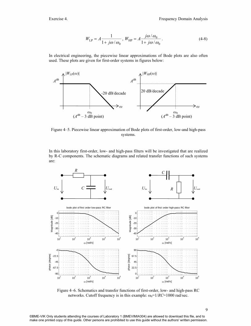
In electrical engineering, the piecewise linear approximations of Bode plots are also often used. These plots are given for first-order systems in figures below:

Figure 4–5. Piecewise linear approximation of Bode plots of first-order, low-and high-pass

systems.

In this laboratory first-order, low- and high-pass filters will be investigated that are realized by R-C components. The schematic diagrams and related transfer functions of such systems are:

101 102 103 104 105

-40

-30

-20

-10

0

ω [rad/s]

Mag

nitu

de [d

B]

bode plot of first order low-pass RC filter

101 102 103 104 105-90

-67.5

-45

-22.5

-0

ω [rad/s]

phas

e [d

egre

e]

101 102 103 104 105

-40

-30

-20

-10

0

ω [rad/s]

Mag

nitu

de [d

B]

bode plot of first order high-pass RC filter

101 102 103 104 1050

22.5

45

67.5

90

ω [rad/s]

phas

e [d

egre

e]

Figure 4–6. Schematics and transfer functions of first-order, low- and high-pass RC

networks. Cutoff frequency is in this example: ω0=1/RC=1000 rad/sec.

ω ω0

|WLP(ω)|

-20 dB/decade

AdB

(AdB – 3 dB point)

ω

|WHP(ω)|

AdB

ω0

20 dB/decade

(AdB – 3 dB point)

R

C Uin Uout

C

Uin Uout R



10

The transfer functions of first-order RC networks in analytical forms are:

RCj

Wω+

=1

1RCLP, ,

RCjRCjWω+

ω=

1RCHP, . (4-8)

One can see that the cutoff frequency is: ω0=1/RC, and the nominal gain of these systems is unity, i.e., A = 1. Important properties of these networks are:

property low-pass RC network high-pass RC network

Cutoff frequency / time constant ω0 = 1/τ = 1/RC ω0 = 1/τ = 1/RC

DC gain 0 dB (1) -∞ dB (0)

gain at cutoff frequency -3 dB (1/ 2 ) -3 dB (1/ 2 )

gain at ω→∞ -∞ dB (0) 0 dB (1)

slope of W below cutoff frequency 0 dB/decade 20 dB/decade

slope of W above cutoff frequency -20 dB/decade 0 dB/decade

DC phase shift 0○ 90○

phase shift at cutoff frequency 45○ 45○

phase shift at ω→∞ 90○ 0○

The knowledge of basic behavior of low- and high-pass networks is also important when instruments are characterized. For example, when an oscilloscope is used with AC coupling, its input stage behaves like a high-pass filter. The cutoff frequency of AC coupling of the oscilloscope Agilent 54622 is 3.5 Hz by specification.

For high-frequency signals an instrument (oscilloscope, mulimeter…) behaves like a low-pass filter. Care should be taken, since not only the fundamental, but higher order harmonic components can be modified by the instrument. For example, if the bandwidth of an oscilloscope is 100 MHz, and a periodic square wave of 10 MHz is measured, the effect of the oscilloscope’s bandwidth even on the 10-th (and higher order) harmonic components can not be neglected. It will result in the phenomena as the square wave would be composed of only harmonic components up to the order of ten, hence sharp edges will disappear. The bandwidth of some oscilloscopes can also be decreased intentionally to improve signal-to-noise ratio when low frequency signals are measured.

The time domain behaviors of first-order RC networks are shown in the figures below:



11

0 1 2 3 4 5 6 7 8 9 10

0

0.2

0.4

0.6

0.8

1

time [ms]

ampl

itude

step response of low-pass RC filter

0 1 2 3 4 5 6 7 8 9 10

0

0.2

0.4

0.6

0.8

1

time [ms]

ampl

itude

step response of high-pass RC filter

Figure 4–7. Step responses of first-order, low- and high-pass RC networks. Time constant is:

τ=1/ω0=RC=1 msec.

Web Links

http://en.wikipedia.org/wiki/Cutoff_frequency

http://en.wikipedia.org/wiki/Oscilloscope

http://en.wikipedia.org/wiki/Frequency_domain

http://en.wikipedia.org/wiki/Fourier_transform

Measurement Instruments

Digital multimeter Agilent 34401A

Power supply Agilent E3630

Function generator Agilent 33220A

Oscilloscope Agilent 54622A



12

Test Board

The board VIK-05-01 contains objects to be measured. The RC networks are configurable by allowing to select the resistance. The time constants for both the low- and high-pass networks are can be set by knobs.

Figure 4–8. Circuit diagram of the variable first-order, low-pass filter

Figure 4–9. Circuit diagram of the variable first-order, high-pass filter



13

Laboratory Exercises

1. Spectrums Generate sine, triangular, square periodic waves by using the function generator. Display spectrums of these signals on the oscilloscope (use the built-in FFT function).

1.1. Measure at least 10 harmonics of the periodic signals and compare to theoretical values. What are the differences? What is the reason?

Let the amplitude be 2 Vpp in every case. The output load of the function generator should be high impedance, otherwise the displayed values on the generator and the oscilloscope are different. It is worth knowing that the oscilloscope displays the result of the FFT in dBV which means that the reference is a sine signal with amplitude 1 V rms.

1.2. Change the duty cycle of the square wave. What does it cause in the spectrum?

Note: low value for duty cycle can be set up in the Pulse menu.

1.3. Study the spectrum of a noise signal. Examine the differences with other waves.

2. Analysis of Low-pass and High-Pass Filtering Determine effects of low-pass and high-pass filtering in time and frequency domain, respectively. During the measurement use square wave, and use the oscilloscope.

2.1. Use the first-order, low-pass filter of the test board. Applying square wave excitation examine the output signal in time and frequency domain, respectively. What is the experience? Explain the results!

It is worth setting up the frequency of the square wave after calculating the cutoff frequency (see the figure 4-8/9.).

2.2. Repeat the previous exercise using a high-pass filter on the same board. Let the frequency be approximately 10 times smaller than the cutoff frequency of the filter. What is the effect of the filter on the square wave?

2.3. Study the behavior of the oscilloscope in the case of a very low frequency square wave. Check the effect of switching between AC and DC coupling. What is the reason of the difference?

2.4. Measure a very high frequency square wave in the time domain. What is the difference compared with the ideal square wave? Why?

3. Measuring amplitude characteristic by applying sine excitation Measure the amplitude characteristic of the first-order, low-pass filter. Use the sine wave generator and the AC voltmeter. Display input and output signals on the oscilloscope.

3.1. Let the measurement range be between 2 decades lower and 1 decade over the theoretical cutoff frequency. Use approximately logarithmic frequency scale.

A possible, approximately logarithmic frequency scale is 1, 2, 5, 10-times the theoretical cutoff frequency. For lower frequencies the same scale can be used.

3.2. Determine the real cutoff frequency by measuring the -3 dB point.



14

4. Measuring amplitude characteristic by applying high bandwidth periodic signals Measure the amplitude characteristic of the first-order, low-pass filter on the board in one step. The parameters of the filter (values of the resistors) can be set up by the switch.

4.1. Estimate the cutoff frequency by examining the input and output spectrums. The excitation signal should be sine or multi sine wave. Determine the time constant from frequency domain measurements! What kind of errors have effect on the accuracy?

4.2. Use noise signal as excitation. Measure the amplitude spectrum of the output.

5. Measurement of non-linear distortion. Measure the distortion of a sine wave.

5.1. Study the waveforms in time and frequency domains. In which domain can the distortion be detected easier?

5.2. Calculate the distortion using the measured harmonics.

Additional Laboratory Exercises

6. Spectrums of arbitrary periodic signals 6.1. Following guides of the instructor design a periodic signal and download into

the arbitrary function generator.

6.1.1. Check the spectrum by using the Fourier analyzer.

7. Measurement of the amplitude characteristic 7.1. Measure the amplitude characteristic of an unknown filter circuit.

7.1.1. Use sine wave generator and AC volt meter. Determine the cutoff frequency.

7.1.2. Repeat the measurement by applying a selected excitation signal and FFT. What kind of excitation signal should be used?

8. Fourier analyzer 8.1. Study the properties of Fourier analyses.

8.1.1. What is the effect of sampling? Which parameters have influences on the frequency resolutions?

8.1.2. In which cases does leakage occur? How can it be avoided? Why are windows used?

Additional remarks

Measurement of the spectrum

The spectrum of signals can be measured with spectrum analyzers. There are dedicated instruments for spectrum analysis, but several modern oscilloscopes also have built-in FFT (Fast Fourier Transform) based spectrum analyzer. In the laboratory, the FFT module of the



15

oscilloscope is used to display the spectrum. FFT is a special case of the well-known DFT (Discrete Fourier Transform). In the FFT, the symmetry of exponential basis functions are used to improve the speed of spectrum calculation.

When a spectrum analyzer is used to display the spectrum of a signal, generally one-sided spectrum is displayed, i.e., only the positive (right) frequency axis is displayed (note that in Table 4-II both negative and positive frequency axes are displayed). This means no loss of information since the spectrum lines at the negative axis are the complex conjugates of the positive ones, so the amplitude spectrum is symmetric, and positive part is enough for most of the analysis.

Since digital oscilloscopes work on sampled signals, so sampling theorem should be hold, i.e., the bandwidth of the observed signal should be less than the half of the sampling frequency.

An important aspect of FFT-based spectrum analysis is that a real instrument can process samples of finite length. It is called windowing, i.e., the processing of finite number of samples of a signal means that we select a finite time window from the whole signal. Two important result of this fact are the so called leakage and picket fence. Leakage means that spectrum components may appear on such frequencies where no signal is present, and picket fence means that the amplitude of a signal obtained after FFT may smaller than its real amplitude. Windowing appears in each case since observation of a signal over an infinite time interval is practically not possible.

0 5000-2

0

2

time

ampl

itude

0 0.050

0.5

1

frequency

ampl

itude

0 5000-2

0

2

time

ampl

itude

0 0.050

0.5

1

frequency

ampl

itude

4800 5000 5200-2

0

2

time

ampl

itude

0 0.02 0.04 0.06 0.080

0.5

1

frequency

ampl

itude

Figure 4–10. Illustration of the effect of windowing. The first row contains the time

functions while the second row contains corresponding spectrums. Left column: ideal sine wave and its spectrum. Center column: the observed (windowed) part of a sine wave and its

spectrum. Right column: the FFT of the observed signal. Circles indicate the spectrum calculated by FFT, the dotted line is the spectrum of the windowed signal. Both picked fence

and leakage can be observed. Frequency of the signal is 0.025 Hz and sampling frequency is 1 Hz.

The complete explanation of the phenomenon of windowing is out of the scope of this guide but a short illustration of the leakage and picket fence can be seen in Fig. 4–10. for the case of a pure sine wave.



16

The left column of Fig. 4–10. shows the time function of a rather long observation of a sine wave (it is a good approximation of an infinite long observation). The spectrum is a spike at the frequency of the signal (0.025 Hz), as expected.

In the center column, a finite interval is selected from the time function. This operation can be mathematically modeled as if the signal were multiplied by a window function w(t) which is zero where the signal is not observed and it is one where the signal can be observed. This kind of window function is called rectangular window. The spectrum of such a truncated sine wave is not a Dirac pulse, but the spectrum of the window function at the frequency of the sine wave (in the case of a rectangular window, it is a discrete sinc function). The reason is that multiplication in time domain corresponds to convolution in frequency domain: let the Fourier transform of the window function be W(f) and the spectrum of the sine wave is δ(f–f0), hence their convolution is W(f)×δ(f–f0) = W(f–f0).

Finally, the FFT can be interpreted as if the continuous spectrum were sampled at discrete frequency values (it is a discrete Fourier transform). The values calculated by the FFT from the windowed signal are indicated by circles in the right column of Fig. 4–10 (these values are displayed on a spectrum analyzer). As one can see, in worst case the spectrum is calculated not at the peak of the windowed spectrum, so the peak value displayed by the spectrum analyzer is smaller than the peak value of the original spectrum. This phenomenon is called picket fence. The leakage can also be recognized in the figure, since the spectrum calculated by FFT contains nonzero values around the peak of the spectrum, where the spectrum of an ideal sine wave is zero.

The effect of picket fence and leakage can be reduced by applying different window functions. There are several window functions, most commonly used windows are: rectangular window, Hanning window and flat-top window.

4800 4900 5000 5100 5200

-2

-1

0

1

2

time

ampl

itude

0 0.02 0.04 0.06 0.080

0.5

1

frequency

ampl

itude

4800 4900 5000 5100 5200

-2

-1

0

1

2

time

ampl

itude

0 0.02 0.04 0.06 0.080

0.5

1

frequency

ampl

itude

4800 4900 5000 5100 5200

-2

-1

0

1

2

time

ampl

itude

0 0.02 0.04 0.06 0.080

0.5

1

frequency

ampl

itude

Figure 4–11. Spectrums with different window functions: rectangular, Hanning, flat-top.

Frequency of the signal is 0.025 Hz and sampling frequency is 1 Hz.

Fig. 4–11. shows the spectrum of a sine wave with different window functions. The leakage is most serious in the case of the rectangular window. In worst case, the amplitude of the signal read from the spectrum analyzer can be even approximately 65% (approx. 4 dB) of the original amplitude (see left columns). In the case of a flat-top window (right column), the amplitude of the signal is displayed correctly, i.e., picket fence practically disappears, so it is advantageous when amplitude is measured. Its disadvantage is that the peak at the frequency of the sine wave becomes rather wide. A good trade-off is Hanning window which is often used for general investigations.



17

Let’s note that windowing occurs even we do not use it intentionally, but we process a data set of finite length without explicitly windowing it. In this case we use rectangular window implicitly.

It is also important, that picket fence and leakage can disappear even in the case of a rectangular window, but it depends on the frequency of the signal to be observed (compare Fig. 4–11 and Fig. 4–12). This is the real problem, since if the picket fence would reduce the amplitude to 65% in every case, this error could be compensated, but the amount of amplitude reduction depends on the signal’s frequency so it is hard/impossible to compensate.

4800 4900 5000 5100 5200

-2

0

2

time

ampl

itude

0 0.02 0.04 0.06 0.080

0.5

1

frequency

ampl

itude

4800 4900 5000 5100 5200

-2

0

2

time

ampl

itude

0 0.02 0.04 0.06 0.080

0.5

1

frequency

ampl

itude

4800 4900 5000 5100 5200

-2

0

2

time

ampl

itude

0 0.02 0.04 0.06 0.080

0.5

1

frequency

ampl

itude

Figure 4–12. Spectrums with different window functions: rectangular, Hanning, flat-top.

Frequency of the signal is 0.024 Hz and sampling frequency is 1 Hz. There is no picket fence and leakage.

Bandwidth

Every real measurement device has a finite input bandwidth, so does the oscilloscope. Within the bandwidth, input signals are handled unbiased. In the case of DC coupling the input characteristic can be modeled by a first-order, low-pass filter. The definition of the bandwidth is the frequency where the power has dropped by half (-3 dB). If the input signal contains components out of this band, then the measured signal will be distorted. The error can be detected in both frequency (assuming that the device has FFT function) and time domains, because the FFT is based on time-domain measured data. In case of sine waves the situation is simple. However, before measuring complex signals (square, triangular signals) the frequency bandwidth which guarantees undistorted transfer has to be estimated.

Dynamic range

Applying frequency domain measurements two important parameters of the measurement devices have to be considered: bandwidth and dynamics. The dynamics is not equivalent with the resolution of the AD converter. The former gives the difference which can be measured between two signals (during one measurement session). The later one defines the smallest step size. The smallest signal that can be measured is typically determined by the noise floor, which may coincide with error derived by resolution of the AD converter or may be greater because of analog noise sources or may be decreased by using averaging. The dynamic of a common measurement device is 50-60 dB. In the case of a high quality spectrum analyzer it can be even 90 dB.



18

Sampling frequency

In digital devices the sampling frequency is one of the most important parameters. Unfortunately, the requirement in time domain differs from the requirement in frequency domain. Measurement in frequency domain needs only the sampling theorem to be complied. For example, in the case of sine waves 4-5 samples from one period are enough. In the case of time domain analysis more samples are necessary. To observe small changes in waves as high sampling frequency as possible should be applied. However, in frequency domain the frequency resolution should be increased. In the case of FFT analyzers distance between two adjacent frequencies depends on the size of FFT and the sampling frequency ( Nff s=Δ ). According to the expression increasing the sampling frequency decreases the resolution. A good strategy in frequency domain analysis is when we decrease the sampling frequency as much as possible while we increase the size of FFT. It is worth noting that the device in the laboratory works with fixed size of FFT. Therefore, only the sampling frequency can be adjusted.

Test questions

1. What are the spectrums of the following waves: sine, square and triangle waveforms?

2. What is the spectrum of a square pulse?

3. Let the period time be fixed. What causes varying the rise and fall time of a triangle wave in the spectrum?

4. Let the period time be fixed. What causes varying the duty cycle of a square wave in the spectrum?

5. What is the equivalent operation of time shifting in the frequency domain?

6. What is the spectrum of the convolution of two given signals?

7. What is the spectrum of the derivative of a given signal?

8. What is the spectrum of the integral of a given signal?

9. What is the effect of scaling the time ( ( ) ( )atxtx ⇒ , a is a constant) in the spectrum?

10. How can the power be calculated in time and frequency domain, respectively?

11. What kind of frequency components can be observed in the output if a linear system is excited by a symmetric square wave?

12. What kind of frequency components can be observed in the output if a non-linear system is excited by a symmetric square wave?

13. What is the spectrum of a real and absolutely integrable signal?


frequency domain analysis

Documents

fourier series of signals

frequency domain analysis

frequency domain tools

frequency domain ones

fourier transform

practical signals

timedomain representation

angular frequency