dynamic circuits: frequency domain analysis

1

Electronic Circuits 1

Dynamic circuits:Frequency domain analysis

Prof. C.K. Tse: Dynamic circuits:Frequency domain analysis

Contents• Free oscillation and natural frequency• Transfer functions• Frequency response• Bode plots

2Prof. C.K. Tse: Dynamic circuits:

Frequency domain analysis

System behaviour: overview



System behaviour : review

♦ solution = transient + steady state

♦ Mathematically,♦ Transient = complementary function (solution of the system

when the sources are zero♦ Steady state = particular solution when the sources are applied

natural response(system characteristic, c.f.personality of a person)

forced response(system altered by external force,

c.f. personality changes due topeer influence)



Natural response (free oscillation)

♦ The natural response is important because it gives thecharacteristic of the circuit.

♦ The characteristic (like stability, transient speed, etc.) ofthe system can be studied by looking at its naturalresponse.

♦ Natural response has nothing to do with the external forces. Hence,we can just look at the circuit with ALL SOURCES reduced to zero.♦ Short circuit all voltage sources♦ Open circuit all current sources

The resulting circuit is called the FREE OSCILLATING circuit.



Free oscillating version of a circuit

Free oscillating circuit

Natural response:



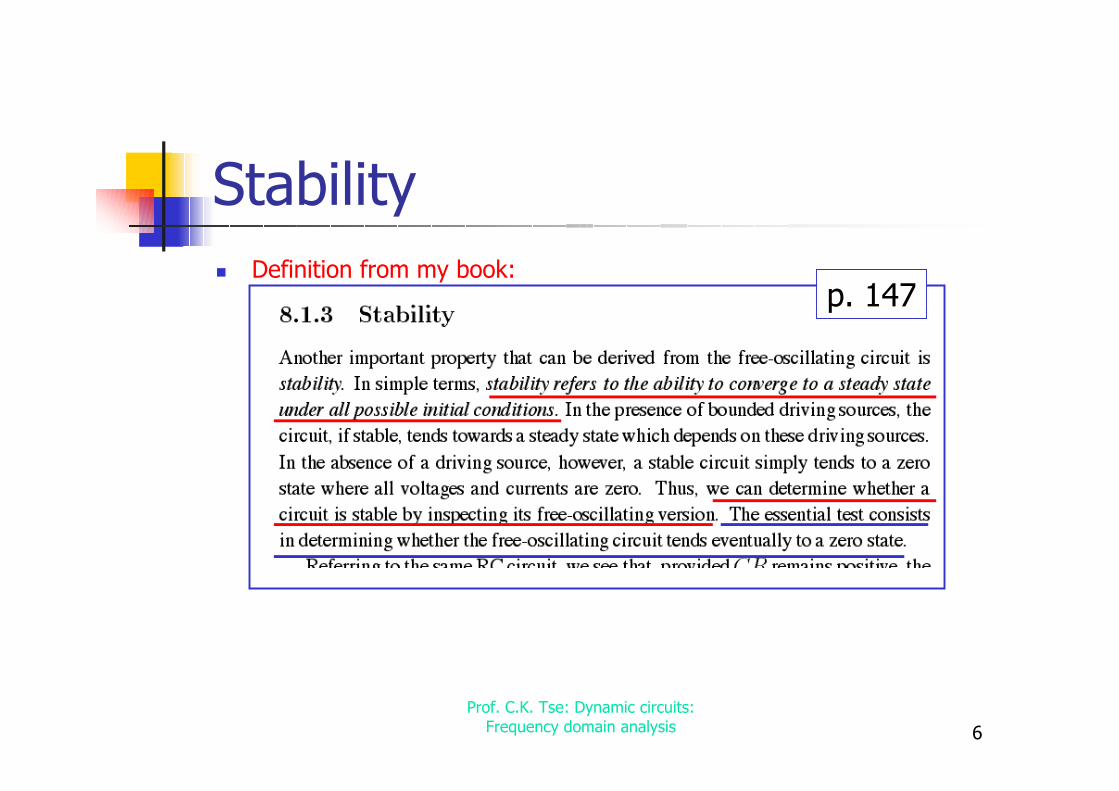
StabilityDefinition from my book:

p. 147



Stability test

Inspect the free oscillating circuitFind its solution (i.e., natural response)Check if the solution goes to zero as time tends to ∞.

Test procedure:

Suppose the system is:

The solution is:

Here, λi are eigenvalues (natural frequencies) which can be real or complex.

Clearly, stability requires that ALL λi are negative or having negative realparts.



Example: first-order response

The free-oscillating response is:

The system is stable if λ < 0; otherwise it is unstable.

stable unstable



Example: second-order responseThe free-oscillating response is:

Case 1: eigenvalues are realStable if λ1 and λ2 are both negative.

Case 2: eigenvalues are complex, i.e.,Solution is

Stable if α is negative

x t A e A et t( ) = +1 21 2λ λ

λ α ω1 2, = ± j

x t e A t B tt( ) ( sin cos )= +α ω ωstableunstable



Stability and characteristic equation

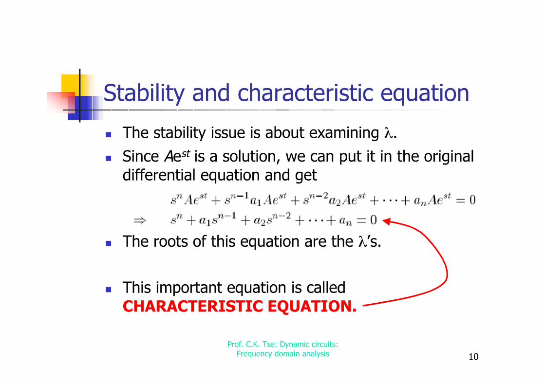
The stability issue is about examining λ.

Since Aest is a solution, we can put it in the originaldifferential equation and get

The roots of this equation are the λ’s.

This important equation is calledCHARACTERISTIC EQUATION.



ExampleSuppose we wish to study the stability of this circuit.We look at the free-oscillating circuit:

State equation is:

or

The characteristic equation is



Example

Solving the characteristic equation gives

Clearly, if R, L and C are positive, then all λ’s are negative.



Natural frequenciesNatural frequencies = eigenvalues, λk

Roots of characteristic equation

For an nth order system, there are n natural frequencies.

The system solution is

complex

Exponential decayExponential growth (unstable)

OscillatoryOscillatory with decaying amp

Oscillatory with growing amp (unstable)

dynamical modes



The complex frequency planejω

σ

t

Exponential decay

t

Exponential growth

x

x sine wave

s-plane

x

x

x

x



SourcesSuppose a voltage has a complex frequency s.

v(t) = Vo est

If s = ±jω, then it is pure sinusoidal since

Sine waves have pure imaginary frequencies, ±jω rad/sec.

cosω

ω ωt

e ej t j t=

+ −

2



ImpedancesWe can also extend the concept of complex frequency to impedance.

Recall: in last lecture, we said that• the impedance of an inductor is jωL when it is driven by a sinesource.• the impedance of a capacitor is 1/jωC when it is driven by asine source.

Now, we imagine the driving frequency is s. Thus, we have

ZL = sLZc = 1/sC

VL = sL ILIC = sC VC



ExampleConsider the impedance:

Thus, we can write:

The free-oscillating circuit will have

The characteristic equation is

The natural frequency (eigenvalue) is λ = 1/CR which is 1/τ.



Transfer functionsTransfer function — ratio of two quantities1. Voltage gain: v2/v12. Current gain: i2/i1 3. Trans-admittance: i2/v14. Trans-impedance: v2/i1

+–V1

driven at s

I2F(s) = I2(s)/V1(s)

in the s domain

all voltages and currents are set to frequency s

linear circuit



ExampleSuppose the circuit is driven by V1 at frequency s.

So, the inductor impedance = sL the capacitor impedance = 1/sC

We can redraw the circuit as

The transfer function from V1 to V2 is



Getting characteristic equation from transfer function

The transfer function from V1 to V2 is

Clearly, the free-oscillating circuit can be formed by setting V1=0.

Thus, the characteristic equation is just

= 0

In general,

F(s) =

Char. Eqn. is

D(s) = 0



Transfer function on complex plane

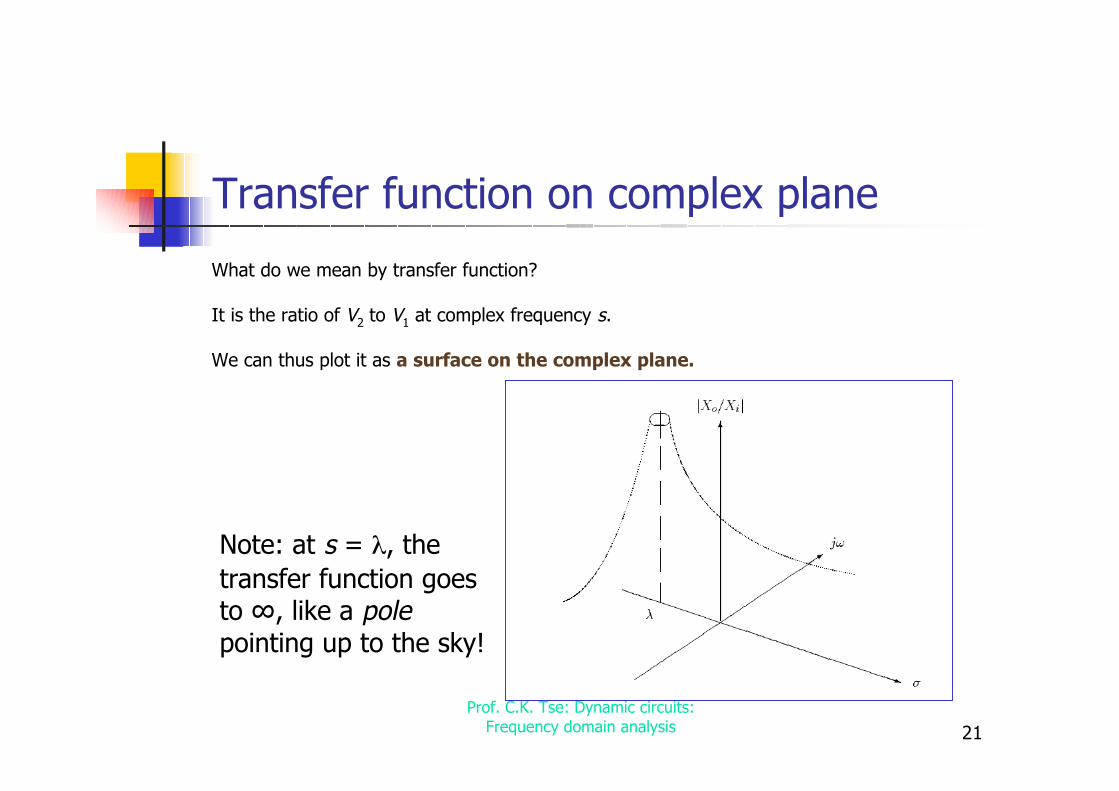
What do we mean by transfer function?

It is the ratio of V2 to V1 at complex frequency s.

We can thus plot it as a surface on the complex plane.

Note: at s = λ, thetransfer function goesto ∞, like a polepointing up to the sky!



Meaning of transfer function

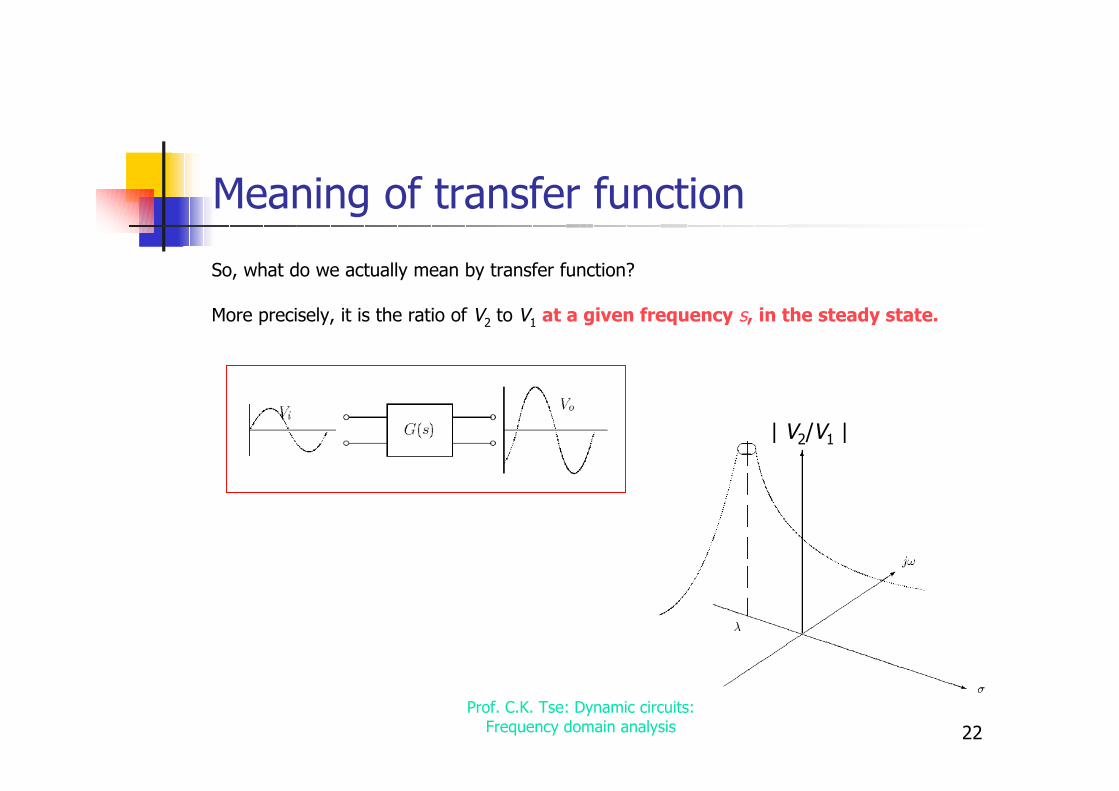
So, what do we actually mean by transfer function?

More precisely, it is the ratio of V2 to V1 at a given frequency s, in the steady state.

| V2/V1 |



Frequency responseIn particular, if we put s = jω, the input is a sinusoidal driving source.In other words, we are looking at the cross section of the surface when it iscut along the imaginary axis (y-axis).

| V2/V1 |



Frequency response vs. transientConsider a simple first-order system.

The frequency response has a pole at s = λ.The transient is A exp (λt).

So, there is correspondence between frequency response and transient.

| V2/V1 |

v2(t) = Aeλt1s + λ

t



More examples

time domain frequency domain

Recall: Laplace transform pairs



First-order low-pass frequency response

The transfer function of a first-order low-passRC filter is

G sV sV s

sCR sC sCR

( )( )( )

//

= =+

=+

2

1

11

11

Hence, 1. this transfer function has a pole at

p

CR= −

1

2. for large magnitudes of s (i.e., |s\ → ∞), G(s) goes to 0.

(At this frequency, G(s) goes to ∞.)

From this, we can roughly sketch G(s) on the complex plane.



Rubber sheet analogy

Pole: –1/CRmagnitude goes to ∞.

All surroundings go to 0,for large |s|.



First-order low-pass frequency response




Bandwidth depends on –1/CR



Frequency response close-up

Observations:

If the pole is further away from theorigin, then the frequency responsestarts to drop off at a higherfrequency.

At ω = 1/CR rad/s, the response dropsto 0.7071 of the dc value, which isexactly 3 dB below the dc value.3dB corner frequency

=1/CR

G jj CR C R

( )ωω ω

=+

=+

11

1

1 2 2 2

Exact formula:



Example

Consider a first order circuit having thefollowing transfer function:

The eigenvalue is –10000.

The time domain response of the free-oscillatingsystem is: y(t) = A e–10000t

In the frequency domain, the ratio |Y/X| is 10 at dc,and starts to drop at around 10000 rad/s (or 1.59kHz) which is the 3dB corner frequency.

Y sX s s

( )( )

=

+

10

110000

10000 rad/sor1.59 kHz

10

7.0712.929

|Y/X|



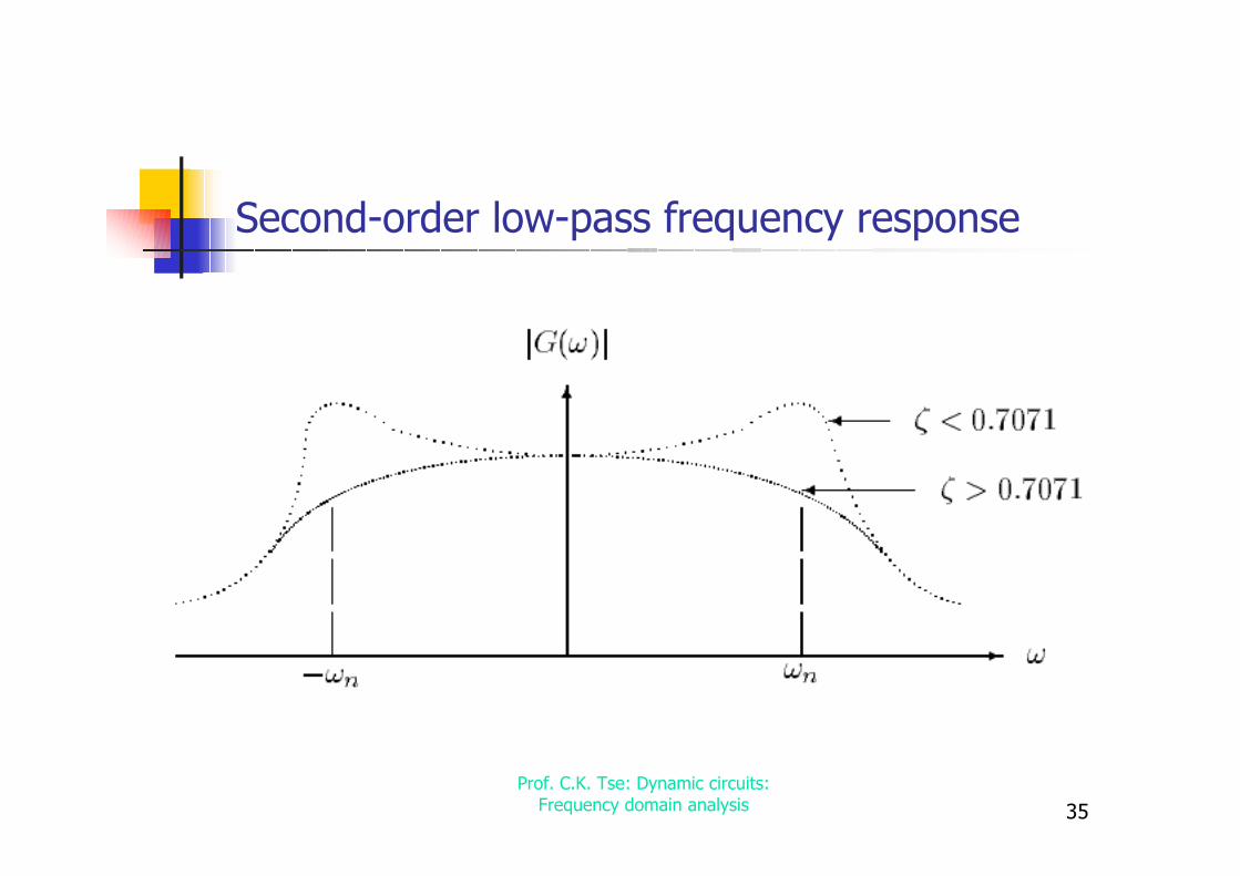
Second-order low-pass frequency response withcomplex pole pair

Consider a second order circuit having thefollowing transfer function:

Suppose the eigenvalues are complex.

The response depends on ζ.

G ss s

n n

( ) =

+ +

1

12 2

2

ς

ω ω

s jn n= − ± −ςω ω ς1 2

Here,ζ is the damping factorωn is the resonant frequency

complex poles

ζ < 0.7071 : light damping — freq response shows a peakingζ > 0.7071 : heavy damping — freq response shows no peakingωn is roughly where the corner frequency is.



Complex pole pair seen on the s-plane

The complex frequency plane is often called the s-plane.



Second-order low-pass frequency response:Rubber sheet analogy



Second-order low-pass frequency response



Resonance: a special case where ζ is small

“Exact” resonance: when drivingfrequency is exactly the naturalfrequency (eigenvalue), the response isinfinitely large!

But, if you can only have sine waves asdriving sources, then you can’t haveexact resonance for systems withcomplex poles.

Near resonance: for systems with ζ <0.7071, the response has a peak aroundω = ω n (actually to be moreaccurate).

For small ζ, we can say that the systemnearly resonates at ω n.

ω ςn 1 2− ω ≈ ω n

small ζ

|G|

ω



LC resonant circuits (theoretical cases: ζ = 0)

ω = ωn

ζ = 0

|Y| or |Z|

ω

L

C

+V(s)

–

I(s) Y s

I sV s

sC

s LC( )

( )( )

= =+1 2

L C+

V(s)–

I(s) Z s

V sI s

sL

s LC( )

( )( )

= =+1 2

In these cases, we see exact resonance because the natural frequencies fall on the imaginary axisand we can find sine wave driving sources. But, the question is “do we have perfect inductor andcapacitor, without resistance?”

Poles are ±jωn

Short-circuit at ω = ωn.

Poles are ±jωn

Open-circuit at ω = ωn.



More example on frequency response

In the steady-state, we can applyconventional analysis (like nodal) to get

G GsL

G

G G G sC

V

V

G Vin1 2 2

2 2 3

1

2

11

0

+ + −

− + +

=

Thus, the input to output transfer function is

For s=0, |V2/Vin| → 0

For s→j∞, |V2/Vin| → 0

So, it’s a bandpass



Poles and zeros: review

In general the transfer function is

Poles — roots of D(s) = 0points on s-plane where |G| goes to ∞.

Zeros — roots of N(s) = 0points on s-plane where |G| goes to 0.

For real systems, the degree of N(s) is always less than or equal tothat of D(s), so that there cannot be more zeros than poles!WHY? Think about what happens when s → ∞.



Example

Poles : –2±j3 and –10points on s-plane where |G1| goes to ∞.

Zeros : 0 and ±j10points on s-plane where |G1| goes to 0.

Also,

Consider

lim | ( ) |s

G s→∞

=1 1




bandpass



Story half told! How about phase?

Frequency response should characterized by- Magnitude- Phase shift

For sinusoidal driving signals, we consider G(jω).

Consider the simple RC circuit.The transfer function is

The phase shift is given by

G jV jV j j CR

( )( )( )

ωω

ω ω= =

+2

1

11

φ ω( )j = −phase shift due to nominator phase shift due to denominator

φ ω ω( ) arctan( )j CR= −0



Full frequency response of RC circuit

φ ω ω( ) arctan( )j CR= −0

G jV jV j j CR

( )( )( )

ωω

ω ω= =

+2

1

11

G jj CR C R

( )ωω ω

=+

=+

11

1

1 2 2 2Mag:

Phase:



Phase response of second-order systemwith a complex pole pair

φ ω

ςω

ω

ω

ω

ςω

ω ω

( ) arctan

arctan

= −

−

−−

0

2

1

2

2

2

2 2

n

n

n

=

Phase:

G jj j

n n n n

( )ωως

ω

ω

ω

ω

ω

ως

ω

=

+ −

=

−

+

1

12

1

122

2

2

2

G ss s

n n

( ) =

+ +

1

12 2

2

ς

ω ω

⇒



Phase response of second-order systemwith real poles

φ ω

ω ω( ) arctan arctan= −

−

1 1000

Phase:

G j

jj

( )

( )

ω

ωω

=

+ +

1

1 11000

G s

ss

( )

( )

=

+ +

1

1 11000

⇒

–90



Plotting frequency response

Direct method:direct substitution of s = jω in the transfer function, and plot themagnitude and phase as a function of frequency.

e.g.,

Magnitude and phase are functions of ω:

Then, we can plot them by any means,e.g., Matlab, mathematica, etc.

G jj CR

( )ωω

=+

11

| ( ) |G jC R

ωω

=+

1

1 2 2 2

θ ω ω( ) arctan= ( )CR



Plotting it with linear scale

| ( ) |G jC R

ωω

=+

1

1 2 2 2

θ ω ω( ) arctan= ( )CR



Plotting frequency response

Problem with scaling

As seen before, the plots are usually nonlinear— some square withina square root, etc. and some arctan function!

The most difficult problem with linear scale is the limited range.

10 20 30 40 50 60 70 … where is 1000?

LINEAR SCALE:



Log scale

If the x-axis is plotted in log scale, then the range can be widened.

1 10 100 103 104 105 106 107 …

LOG SCALE:



Bode technique : asymptotic approximation

Consider the same first-order transfer function

The square of the magnitude is:

Take the log of both sides and multiply by 20:

Define

20 10 1 2 2 2log ( ) log( )G C Rω ω= − +

G jj CR

( )ωω

=+

11

GC R

( )ωω

2

2 2 2

1

1=

+

y Gx

=

=

20log| ( ) |log

ω

ω

The unit of y is the decibel (dB)



Bode technique for plotting frequency response

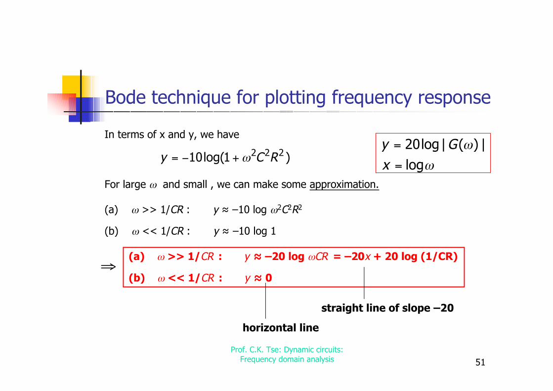
In terms of x and y, we have

For large ω and small , we can make some approximation.

(a) ω >> 1/CR : y ≈ –10 log ω2C2R2

(b) ω << 1/CR : y ≈ –10 log 1

y C R= − +10 1 2 2 2log( )ω

(a) ω >> 1/CR : y ≈ –20 log ωCR = –20x + 20 log (1/CR)

(b) ω << 1/CR : y ≈ 0⇒

y Gx

=

=

20log| ( ) |log

ω

ω

straight line of slope –20

horizontal line



Bode approximation (magnitude)(a) ω >> 1/CR : y ≈ –20x + 20 log (1/CR)

(b) ω << 1/CR : y ≈ 0

The trick is:

If we plot y versus x,then we get straightlines as asymptotesfor large and small ω.

Note:The approximation ispoor for ω near 1/CR.



Bode approximation (phase)

The approximation is

θ ω ω( ) arctan= ( )CRSame example:

θ ω

ω

ω

ω

( )

≈ <<

= − =

≈ − >>

01

451

901

for

for

for

CR

CR

CR

one decade below 1/CR

one decade above 1/CR



Bode plots: general technique

Since Bode plots are log-scale plots, we may plot any transferfunction by adding together simpler transfer functions which makeup the whole transfer function.

G s

s s

s s s( ) =

+×

+

+

+

×

+

12 10

1100

15000

14 10

110

4

6 8

Plot A Plot B

Plot C Plot D Plot E



Bode plots: standard forms

1. Simple pole

2. Simple zero

3. Integrating pole

4. Differentiating zero

5. Constant

6. Complex pole pair

G s

s p( ) =

+

11

G s s z( ) = +1

G s

s p( )

/=

1

G ssz

( ) =

G s A( ) =

G ss s

n n

( ) =

+ +

1

12 2

2

ς

ω ω




Simple pole:

(logscale)

(logscale)




Simple zero:

(logscale)

(logscale)




Integrating pole:(logscale)

(logscale)




Differentiating zero:(logscale)

(logscale)




Constant:

(logscale)

(logscale)




Complex pole pair

(logscale)

(logscale)



Example

simple zero

simple pole

constant

differentiating pole

Note: ω = 2πf

If ω = 200π rad/s,f = 100 Hz.



Example



Semi-log graph paper allows compressed x-axis

1 10 100 103 104 105 106

Effectively, the x-axisis being log’ed0 1 2 3 4 5 6usual label forpractical convenience

dynamic circuits: frequency domain analysis

Documents