frequency domain linearized navier-stokes...

KTH Linne FLOW Centre

Frequency Domain Linearized Navier-StokesEquations Methods for Low Mach Number

Internal Aeroacoustics

Axel Kierkegaard

Doctoral Thesis

Stockholm, Sweden 2011The Marcus Wallenberg Laboratory for Sound and Vibration Research

Department of Aeronautical and Vehicle Engineering

Postal address Visiting address ContactRoyal Institute of Technology Teknikringen 8 Tel: +46 8 790 79 03MWL/AVE Stockholm Email: [email protected] 44 StockholmSweden

Akademisk avhandling som med tillstand av Kungliga Tekniska Hogskolani Stockholm framlaggs till offentlig granskning for avlaggande av teknologiedoktorsexamen fredagen den 27:e maj 2011, 13:00 i sal E3, Osquarsbacke 14,Kungliga Tekniska Hogskolan, Stockholm.

TRITA-AVE-2011:34ISSN-1651-7660

c© Axel Kierkegaard, 2011

ii

Abstract

Traffic is a major source of environmental noise in modern day’s society. Asa result, the development of new vehicles are subject to heavy governmentallegislations. The major noise sources on common road vehicles are enginenoise, transmission noise, tire noise and, at high speeds, wind noise. One wayto reduce intake and exhaust noise is to attach mufflers to the exhaust pipes.However, to develop prototypes for the evaluation of muffler performance isa costly and time-consuming process. As a consequence, in recent years so-called virtual prototyping has emerged as an alternative. Current industrialsimulation methodologies are often rather crude, normally only includingone-dimensional mean flows and one-dimensional acoustic fields. Also, flowgenerated noise is rudimentary modeled or not included at all. Hence,improved methods are needed to fully benefit from the possibilities of virtualprototyping.

This thesis is aimed at the development of simulation methodologies suitableboth as industrial tools for the prediction of the acoustic performance offlow duct systems, as well as for analyzing the governing mechanisms of ductaeroacoustics. Special focus has been at investigating the possibilities touse frequency-domain linearized Navier-Stokes equations solvers, where theequations are solved either directly or as eigenvalue formulations.

A frequency-domain linearized Navier-Stokes equations methodology hasbeen developed to simulate sound propagation and acoustic scattering inflow duct systems. The performance of the method has been validated toexperimental data and analytical solutions for several cases of in-duct areaexpansions and orifice plates at different flow speeds. Good agreement hasgenerally been found, suggesting that the proposed methodology is suitablefor analyzing internal aeroacoustics.

iii

Doctoral thesis

This thesis consists of the following papers:

Paper IA. Kierkegaard, S. Boij, and G. Efraimsson. A frequency domain linearizedNavier-Stokes equations approach to acoustic propagation in flow ducts withsharp edges. J. Acoust. Soc. Am., 127(2):710-719, 2010.

Paper IIA. Kierkegaard, S. Boij and G. Efraimsson, Simulations of the Scattering ofSound Waves at a Sudden Area Expansion (submitted).

Paper IIIA. Kierkegaard, G. Efraimsson, S. Allam and M. Abom, Simulations ofwhistling and the whistling potentiality of an in-duct orifice with linearaeroacoustics (submitted).

Paper IVA. Kierkegaard, E. Akervik, G. Efraimsson and D.S. Henningson, Flow fieldeigenmode decompositions in aeroacoustics, Computers & Fluids, 39(2):338-344, 2010.

Conferences

The content of this thesis has been presented at the following conferences:1. A. Kierkegaard S. Boij and G. Efraimsson, Simulations of acoustic

scattering in duct systems with flow, 20th International Congress onAcoustics (ICA), Sydney, Australia, 2010.

2. A. Kierkegaard and G. Efraimsson, Simulations of the whistling poten-tiality of an in-duct orifice with linear aeroacoustics, 16th AIAA/CEASAeroacoustics Conference, Stockholm, Sweden, 2010.

3. A. Kierkegaard and G. Efraimsson, A Numerical Investigation ofInterpolation Methods for Acoustic Analogies, 16th AIAA/CEASAeroacoustics Conference, Stockholm, Sweden, 2010.

4. M. Abom, M. Karlsson and A. Kierkegaard, On the use of linearaeroacoustic methods to predict whistling, 16th International Congresson Sound and Vibration (ICSV 16), Krakow, Poland, 2009.

5. A. Kierkegaard, Simulering av ljudutbredning i rorsystem med gasstrommar,Svenska mekanikdagarna, Sodertalje, Sweden, 2009.

iv

6. A. Kierkegaard, G. Efraimsson and S. Boij, A Frequency DomainLinearized Navier-Stokes Approach to Acoustic Propagation in LowMach Number Flow Ducts, 7th International Workshop for Acousticsand Vibration in Egypt (IWAVE), Cairo, Egypt, 2009.

7. A. Kierkegaard S. Boij and G. Efraimsson, Scattering matrix evaluationwith CFD in low Mach number flow ducts, Society of AutomotiveEngineering, Noise, Vibrations and Harshness Conference, Chicago,USA, 2009.

8. M. Abom, M. Karlsson and A. Kierkegaard, On the use of linear aeroa-coustic methods to predict whistling, Noise and Vibration: EmergingMethods (NOVEM), Oxford, UK, 2009.

9. A. Kierkegaard, G. Efraimsson and S. Boij, Acoustic propagation ina flow duct with an orifice plate, ISMA Conference, Leuven, Belgium,2008.

10. A. Kierkegaard and G. Efraimsson, Generation and Propagationof Sound Waves in Low Mach Number Flows, 13th AIAA/CEASAeroacoustics Conference, Rome, Italy, 2007.

11. A. Kierkegaard and G. Efraimsson, Generation of sound via the useglobal eigenmodes, 5th ERCOFTAC SIG 33 Workshop, Laminar-Turbulent Transition Mechanisms, Prediction and Control, Stockholm,Sweden, 2006.

12. A. Kierkegaard, G. Efraimsson, J. Hœpffner, E. Akervik, D. Henningsonand M. Abom, Identification of sources of sound in low Mach numberflows by the use of flow field eigenmodes, 13th International Congresson Sound and Vibration (ICSV 13), Vienna, Austria, 2006.

Acknowledgments

This work has partly been performed within the Linne FLOW Centre andpartly within the research project ”Reduction of external noise for dieselpropulsed passenger cars”, sponsored by EMFO (Dnr AL 90B2004: 156660)and Vinnova/Green Car (Dnr 2005-00059) with the participating partnersSaab Automobile AB, KTH and Chalmers. The funding is gratefullyacknowledged.

In addition, I would like to show gratitude to my supervisors Assoc.Prof. Gunilla Efraimsson and Prof. Mats Abom for their support andencouragement.

v

Contents

1 Introduction 11.1 Background . . . . . . . . . . . . . . . . . . . . . . . . . . . . 31.2 Acoustic network modeling . . . . . . . . . . . . . . . . . . . 51.3 CAA of flow duct noise . . . . . . . . . . . . . . . . . . . . . 81.4 Fan duct radiation . . . . . . . . . . . . . . . . . . . . . . . . 10

1.4.1 Frequency domain implementations of the LEE . . . . 121.4.2 Other modeling approaches . . . . . . . . . . . . . . . 13

1.5 Kelvin-Helmholtz instabilities . . . . . . . . . . . . . . . . . . 14

2 The linearized Navier-Stokes equations 162.1 Derivation of the linearized Navier-Stokes equations . . . . . 182.2 Boundary conditions . . . . . . . . . . . . . . . . . . . . . . . 202.3 Forcing functions . . . . . . . . . . . . . . . . . . . . . . . . . 212.4 Frequency scalings . . . . . . . . . . . . . . . . . . . . . . . . 222.5 The scattering matrix formalism . . . . . . . . . . . . . . . . 232.6 Plane wave decomposition methods . . . . . . . . . . . . . . . 25

2.6.1 Density-velocity method . . . . . . . . . . . . . . . . . 252.6.2 Curve-fitting method . . . . . . . . . . . . . . . . . . . 26

3 Validation cases 293.1 Thin orifice plate . . . . . . . . . . . . . . . . . . . . . . . . . 29

3.1.1 Geometry . . . . . . . . . . . . . . . . . . . . . . . . . 293.1.2 Mean flow . . . . . . . . . . . . . . . . . . . . . . . . . 303.1.3 Perturbation simulations . . . . . . . . . . . . . . . . . 313.1.4 Comparison with experimental data . . . . . . . . . . 33

3.2 Area expansion . . . . . . . . . . . . . . . . . . . . . . . . . . 353.2.1 Geometry . . . . . . . . . . . . . . . . . . . . . . . . . 353.2.2 Mean flow . . . . . . . . . . . . . . . . . . . . . . . . . 353.2.3 Perturbation simulations . . . . . . . . . . . . . . . . . 37

vi

3.2.4 End corrections . . . . . . . . . . . . . . . . . . . . . . 393.3 Whistling . . . . . . . . . . . . . . . . . . . . . . . . . . . . . 42

3.3.1 Geometry . . . . . . . . . . . . . . . . . . . . . . . . . 433.3.2 Mean flow . . . . . . . . . . . . . . . . . . . . . . . . . 443.3.3 Whistling potentiality . . . . . . . . . . . . . . . . . . 453.3.4 Nyquist stability criterion . . . . . . . . . . . . . . . . 47

4 Global modes 504.1 A reduced model of the flow field . . . . . . . . . . . . . . . . 514.2 Open cavity . . . . . . . . . . . . . . . . . . . . . . . . . . . . 524.3 Curles equation . . . . . . . . . . . . . . . . . . . . . . . . . . 53

4.3.1 Application to global modes . . . . . . . . . . . . . . . 554.3.2 Implementation . . . . . . . . . . . . . . . . . . . . . . 57

4.4 Results . . . . . . . . . . . . . . . . . . . . . . . . . . . . . . . 58

5 Conclusions and future work 61

6 Summary of papers 63

Bibliography 67

vii

Chapter 1

Introduction

The field of internal low Mach number aeroacoustics has many applicationswith connection to peoples’ everyday lives. Examples range from unwantednoise such as exhaust noise from cars and building ventilation noise, to thepleasant sounds of flutes and other wind instruments. All examples arehowever governed by the same physical mechanisms. These mechanisms arecommonly divided into two categories; the generation of sound by air flows,and the propagation of sound waves in duct systems with mean flows.

Aside from the appreciated sounds of wind instruments, the large part ofpeoples daily contact with aeroacoustic sound is of the unwanted type, withtransport noise as a primary source of environmental noise. Except for beingpurely annoying, the World Health Organization [1] identifies transport noiseas a source of several health issues, including noise-induced hearing loss, sleepdisturbance effects, increased blood pressure, cardiovascular disease and otherphysiological effects.

The report claims 30 % of EU’s citizens to be exposed at night to equivalentsound pressure levels exceeding 55 dB(A). In contrast, it is stated that fora good night’s sleep, sound levels of continuous background noise shouldnot exceed 30 dB(A) to avoid consequences such as the above mentionedhealth issues and reduction of sleep quality resulting in increased fatigue anddecreased day-after performance.

In addition, it is reported that ”mainly in workers and children, that noisecan adversely affect performance of cognitive tasks.” and ”Reading, attention,

1

problem solving and memorization are among the cognitive effects moststrongly affected by noise.” Children in schools situated in locations withhigh levels of environmental noise is reported to ”under-perform in proofreading, in persistence on challenging puzzles, in tests of reading acquisitionand in motivational capabilities”. In [2], focus is turned on the special caseof low frequency noise, defined as the range of 10 Hz to 200 Hz. Noise in thisfrequency range is identified as particularly harmful to cognitive tasks.

All in all it can be concluded that road traffic is the major source ofenvironmental noise in modern day society. The major noise sources oncommon road vehicles at low speeds are engine noise and tire noise, with tirenoise exceeding engine noise at speeds higher than 40-60 km/h [1]. At highspeeds, wind noise is also an apparent noise source.

Due to the above mentioned problems related to traffic noise, development ofnew vehicles are subject to strict governmental legislations. One common wayto reduce engine noise is to attach mufflers to the exhaust pipes. However, todevelop prototypes of mufflers for evaluation is a costly and time-consumingprocess where the design often has been based on experience and trialand error techniques. As a consequence, in recent years so-called virtualprototyping has emerged, in which computational models are used to optimizemuffler designs. Current industrial simulation methodologies are oftenrather crude, either neglecting mean flows or including only one-dimensionalmean flows and one-dimensional acoustic waves. Hence, improved, but stillefficient, methods are needed to fully benefit from the possibilities of virtualprototyping.

Examples of available commercial software includes AVL BOOST, GTPOWER and SIDLAB. The two first use one-dimensional non-linear equa-tions in time domain to solve coupled flow and acoustic propagation in ductsystems. A benefit of the non-linear simulation technique is the possibilityof calculations at high acoustic amplitudes, but a limitation is the one-dimensional modeling of geometries, which in reality often consists of flowsthat are highly two or three dimensional. SIDLAB on the other hand isbased on a so-called acoustic network model, which is a linear frequencydomain model where acoustic systems are separated into several componentswhich are modeled separately and assumed connected by acoustic plane wavepropagation.

Common to all existing commercial duct acoustics software is the lackof satisfying inclusion of flow-acoustic interaction effects on the acousticpropagation. One obvious way to overcome this limitation would be to solve

2

the full non-linear compressible Navier-Stokes equations for the entire mufflersystem. This is however prohibitively computationally expensive and will beout of reach for industrial use in many years to come. Hence, improved,but still efficient methods are needed to fully benefit from the possibilities ofvirtual prototyping.

The aim of this thesis is to explore the usefulness of existing methodsfor simulations of acoustics and fluid dynamics, when applied to internalaeroacoustics, and to develop appropriate methodologies for simulations ofsound wave propagation in duct systems with low speed air flows. An optimalsimulation strategy include the sufficient level of complexity of the involvedphysics, yet neglects too detailed descriptions which demand additionalcomputational resources without adding to the physical understanding ofthe studied subject. Thus improved knowledge of the governing mechanismsof sound wave propagation in flow ducts is needed to find the optimalbalance between computational effort and the complexity of physics thatis incorporated into the model.

1.1 Background

A majority of all research performed in aeroacoustics and computationalaeroacoustics (CAA) has been aimed at the aircraft noise community, startingwith the pioneering works of Lighthill [3]. Commonly, aircraft noise researchtraditionally focus on high Mach number and high Reynolds number free fieldjet flows. In high-speed jets, noise generation is mainly of quadrupole type,caused by unsteady non-linear mechanisms. The methodologies developedin CAA have reflected this, in their focus on time-domain solutions of thenon-linear Navier-Stokes equations, either as Direct Numerical Simulations(DNS) where no turbulence models are included, to turbulence models such asReynolds-Averaged Navier-Stokes (RANS) and Large Eddy Simulation (LES)codes. As examples, but far from a complete list, [4–9] can be mentioned.Despite the growing number of, primarily LES, aeroacoustic studies of jetnoise, no consensus have been found within the research community onthe choice of turbulence modeling techniques and modeling parameters.Numerical simulation of jet noise and sound generation in general is stillfar from a fully explored research area.

In wall-bound and internal flows at low Mach numbers, the sound generatingmechanisms are however governed by fundamentally different physics than

3

that of free-field jet noise. When an airflow is obstructed by a change ofgeometry, such as a sharp corner or a bifurcation, flow instabilities andvortices are generated. As these vortices impinge on boundaries, soundimpulses are generated. In a non-deterministic flow, vortices will impingeon walls at random times and with random intensities, and the accumulatedsound will thus be of broadband character. If however the generated soundis back-scattered to the geometry discontinuity, the vortex shedding mightbe affected to form a resonant feedback system which generate tonal noise,i.e. whistling. The most basic geometry of this type is a rectangular cavity,of which the generated sound has been treated in, for example, [10–14].

A less explored field of aeroacoustics is that of pure wave propagation ininhomogeneous media with arbitrary mean flows, as this is disconnected fromthe noise generation processes. The conceptual difference in the simulationof sound generation and sound propagation is large enough to justify atreatment of the two as separate topics. In regions outside of acousticsources, the acoustic quantities are often small in comparison to the theflow field quantities. It many cases it can also be assumed that the flowfield affects the sound waves, whereas the sound waves does not influencethe flow field. Thus, the perturbations about the mean flow are often smallenough to justify linearization. This enables a two-stage treatment of theacoustic wave propagation: firstly, the mean flow can be calculated withoutthe need to consider any acoustic waves, and secondly, the sound waves canbe calculated as perturbations about the mean flow field.

Also, as a consequence of the linearization, a frequency domain approach canbe taken. Benefits of a frequency-domain approach, as opposite to a time-domain approach, is the significant reduction of computational time in case ofsingle frequency excitation. In this case only one single calculation is needed,as opposite to a time-series in the case of time-domain simulations. Anotherstrong benefit of a frequency-domain approach is its ability to suppressgrowing shear layer instabilities, as no temporal growth can exist when atime-harmonic assumption is taken.

Since most research efforts have been aimed at jet noise generation, whereunsteady simulations are needed, few studies have paid attention to thepossibilities of frequency-domain aeroacoustics. Examples of sound wavepropagation simulations in frequency domain are, e.g. [15, 16] where theLinearized Euler Equations were used, and [17] which implemented theLinearized Lilley’s equation. Neither of these studies have included viscouseffects. However, since viscous losses are non-negligible in duct acoustics dueto viscous dissipation along walls and at sharp edges, modeling of viscous

4

aeroacoustics might be relevant. The work presented in this thesis aims as afirst step to the development of a simulation methodology for aeroacousticsof viscous flows.

To the best of the author’s knowledge, no study has previously beenperformed of scattering of sound in flow ducts with linearized frequencydomain Navier-Stokes solvers. However, frequency domain linearized Eulerequation solvers has been utilized in configurations of related character, andother CAA methods has been investigated for the scattering of sound in flowducts.

1.2 Acoustic network modeling

Most realistic industrial flow duct configurations such as vehicle mufflersor ventilation systems are both large and geometrically complex. A directaeroacoustic simulation of such a system will not be manageable within thenear future considering the development pace of todays computer resources,due to the overwhelming computational costs associated with these types ofsimulations.

To reduce the complexity of acoustic flow duct analysis, an alternativemethod is the concept of the so-called acoustic network model, where ageneral flow duct system is modeled by breaking it down into a sequenceof simple elements such as duct sections, junctions, chambers, expansions etc[18]. In the model, all elements interact acoustically and are connected byduct elements through which only acoustical plane waves propagate. The useof acoustic network models include a range of applications such as automotiveexhaust systems, ventilation systems, gas piping, ship propulsion, powerplants etc.

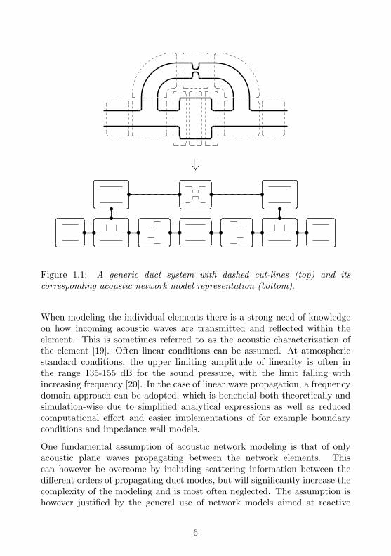
Figure 1.1 (top) shows a generic duct system, in this case an expansionchamber and an area constriction (orifice plate) mounted in parallel by twoT-joints. Dashed lines represents imagined cut-lines to split the duct systeminto more primitive components. Figure 1.1 (bottom) shows an acousticnetwork model representation of the same duct system. Here it can beseen how a complex duct system can be broken down into a network ofsimpler components such as empty duct sections, area expansions and areacontractions. When the scattering by each individual component is known,the acoustic performance of the entire duct system can be determined.

5

⇓

Figure 1.1: A generic duct system with dashed cut-lines (top) and itscorresponding acoustic network model representation (bottom).

When modeling the individual elements there is a strong need of knowledgeon how incoming acoustic waves are transmitted and reflected within theelement. This is sometimes referred to as the acoustic characterization ofthe element [19]. Often linear conditions can be assumed. At atmosphericstandard conditions, the upper limiting amplitude of linearity is often inthe range 135-155 dB for the sound pressure, with the limit falling withincreasing frequency [20]. In the case of linear wave propagation, a frequencydomain approach can be adopted, which is beneficial both theoretically andsimulation-wise due to simplified analytical expressions as well as reducedcomputational effort and easier implementations of for example boundaryconditions and impedance wall models.

One fundamental assumption of acoustic network modeling is that of onlyacoustic plane waves propagating between the network elements. Thiscan however be overcome by including scattering information between thedifferent orders of propagating duct modes, but will significantly increase thecomplexity of the modeling and is most often neglected. The assumption ishowever justified by the general use of network models aimed at reactive

6

silencers where efficient performance is most difficult to reach at lowfrequencies. At typical vehicle engine operating conditions, at around 1500-3000 RPM, the bulk energy is contained within the first few harmonics ofthe cylinder firing frequency, i.e. below a few hundred Hertz [21]. At theselow frequencies, the acoustic wavelengths are typically much larger than thediameters of the ducts connecting the network components and it can withoutmuch loss of generality be assumed that only plane waves propagate betweenthe acoustic network components. At higher frequencies dissipative materialscan be efficiently applied, thus silencer performance optimization is not ascritical for high frequencies as for lower frequencies.

A general network element can be thought of as a black box to which acousticwaves enters and exits through any number of inlets/exits, so-called ports.The general case is referred to as a multi-port [22], or N -port. Here N is thenumber of ducts connected to the component. In the case of area expansionsand other geometry discontinuities, the component is connected to one inflowduct and one outflow duct, and can thus be formulated as an acoustic two-port. Sometimes the term four-pole [23, 24] is used for two-ports. In thecase of a T-joint, three connected ducts are present, and the element is thusrepresented by a three-port, and so on. The methodology is most often usedin the plane wave regime, i.e. below the cut-on frequency of the first higherorder propagating duct mode. Knowledge of the acoustical field inside of theelement is not necessary, only the transfer of acoustic information betweenthe ports of the element. These transfer functions can be represented onvarious formulations and can be achieved either analytically, experimentallyor by simulations.

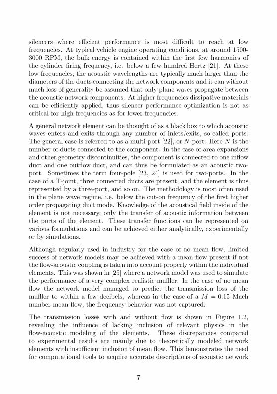
Although regularly used in industry for the case of no mean flow, limitedsuccess of network models may be achieved with a mean flow present if notthe flow-acoustic coupling is taken into account properly within the individualelements. This was shown in [25] where a network model was used to simulatethe performance of a very complex realistic muffler. In the case of no meanflow the network model managed to predict the transmission loss of themuffler to within a few decibels, whereas in the case of a M = 0.15 Machnumber mean flow, the frequency behavior was not captured.

The transmission losses with and without flow is shown in Figure 1.2,revealing the influence of lacking inclusion of relevant physics in theflow-acoustic modeling of the elements. These discrepancies comparedto experimental results are mainly due to theoretically modeled networkelements with insufficient inclusion of mean flow. This demonstrates the needfor computational tools to acquire accurate descriptions of acoustic network

7

Figure 1.2: The transmission loss in decibels of a realistic muffler predictedwith a network model approach in [25]. Without flow (left), and with aM = 0.15 Mach number mean flow (right). Dashed lines represents slightlydifferent modeling approaches, described in [25].

elements with mean flow effects taken into account. This thesis focus onthe acquisition of network element descriptions by the use of computationalaeroacoustics.

1.3 CAA of flow duct noise

Several papers have been published on propagation and scattering ofsound in flow ducts exploring different simulation strategies. In general,advanced and computationally expensive simulation techniques such asDirect Numerical Simulations (DNS) or Large Eddy Simulations (LES) havebeen employed, where the complete non-linear compressible Navier-Stokesequations are solved directly for both mean flow and acoustic and vorticialperturbations simultaneously, with no or little assumptions or turbulencemodeling involved.

One of the more well-studied geometry configurations in internal aeroacous-tics is that of an in-duct orifice. The orifice might be situated along theduct walls, as in the case of duct liners, or as a diaphragm used as a flowconstriction device. Both these cases have many practical applications andare heavily used in industry and thus interesting to study theoretically.

8

For example, DNS was used in [26, 27] to study the dissipation mechanismsof high-intensity acoustic waves due to vortex shedding in an orifice, withapplications to duct liners. Both the conditions without flow [26] andwith gracing flow [27] were investigated, and the former was compared toimpedance-tube measurements.

In [28], DNS was used to simulated the absorption of acoustic energy dueto an in-duct orifice plate without flow and with a laminar M = 0.01 Machnumber through-flow. Reflection and transmission of acoustic waves acrossthe orifice plate were also investigated. A similar study of absorption ofacoustic energy due to an orifice with biased (through-) flow was carried outin [29] and results were compared to an analytical model. LES was used andMach and Reynolds numbers were just slightly higher than in [28]. However,a three-dimensional model was used, as opposite to two-dimensional in allpreviously mentioned studies.

The transmission and reflection of plane waves in a larger duct with an orificeat higher Mach and Reynolds numbers was studied in [30] using unsteadyRANS (u-RANS) simulations, which is less computationally expensivecompared to LES and DNS. Excessive damping of the acoustic waves wasfound in the jet region due to an over-prediction of the turbulent viscosityby the turbulence model. Results of acoustic scattering by the orifice platewere not in good agreement with experimental results and it was concludedthat u-RANS simulations of plane wave propagation in separated flows needto be performed with great care.

In [31], an attempt to predict the sound propagation and generation in atwo-dimensional flow duct with an double orifice configuration by the useof Detached Eddy Simulation (DES) was presented, and simulation resultswere compared to experimental results. However, since no decibel labels wereshown, a quantitative evaluation of simulation accuracy is not possible. ADES was also used in [32] in a semi-three dimensional case of a cut-out ofan eighth of a cylindrical duct with a M = 0.11 Mach number mean flow.The sound generation from an orifice plate placed in a duct upstream of atermination was calculated, and directivity of the sound radiation from theduct exit was compared to measurements.

Sound generation from a slit-shaped orifice in a rectangular duct in threedimensions was studied in [33] in the case of a M = 0.017 Mach numbermean flow. Spectra of fluctuating pressure at various locations both up- anddownstream was presented but not compared to experimental or analyticalresults. However, the simulated spectra were used as reference solution to

9

[34, 35] where a LES simulation was carried out in the near field of anequivalent slit-shaped orifice in a rectangular duct. The Lighthill’s stresstensor was recorded and Fourier transformed pointwise and used as sourceterm in a FEM implementation of the Lighthill analogy in frequency domainto propagate the generated sound out into the far-field of the duct. Largevariations in accuracy was reported depending on method used to interpolatethe sources between the LES and acoustic meshes.

The propagation of sound in a duct with an area expansion at a variousMach number mean flows was studied in [36, 37] where a LES simulation wascoupled to a system identification (SI) technique to characterize the scatteringof the acoustic waves and the results were compared to experimentaldata. The same LES-SI technique was later applied to the case ofscattering of sound by a T-joint with a M = 0.1 Mach number grazingmean flow [38]. A power balance study was carried out to investigate thesound absorption/amplification of the T-joint. Results were compared toexperimental results, which revealed the method’s ability to capture thecorrect physical behavior of the flow-acoustic coupling in the T-joint.

Acoustic scattering at a T-joint was also simulated in [39, 40], however witha different methodology. An incompressible solver was used to calculatethe flow, where velocity perturbations were added at inflow boundariesto mimic incident sound waves. A vortex sound theory integral wasthereafter solved to identify acoustic absorption of amplification to predictflow induced pulsations in piping systems. Although applicable in this case,the methodology is limited to low Helmholtz number cases.

Other integral methods based on amongst other Lighthill’s [3] or Curle’s [41]analogy has been utilized for flow duct sound generation and propagation infor example [42–46]. However, these methods are primarily used for externalsound generation applications and will not be further investigated here.

1.4 Fan duct radiation

Although few papers on CAA for scattering in internal flow ducts has beenpublished, a more extensively explored area with similar requirements onmethodologies, in terms of involved physics, is the field of fan duct radiationwith applications to turbofan engines. Often a given sound source is assumed,and focus is only on the propagation of sound through the engine inlet or thebypass duct and radiation out into open air. A schematic sketch of a typical

10

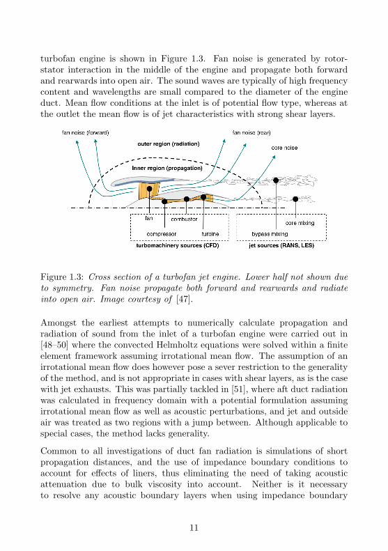
turbofan engine is shown in Figure 1.3. Fan noise is generated by rotor-stator interaction in the middle of the engine and propagate both forwardand rearwards into open air. The sound waves are typically of high frequencycontent and wavelengths are small compared to the diameter of the engineduct. Mean flow conditions at the inlet is of potential flow type, whereas atthe outlet the mean flow is of jet characteristics with strong shear layers.

Figure 1.3: Cross section of a turbofan jet engine. Lower half not shown dueto symmetry. Fan noise propagate both forward and rearwards and radiateinto open air. Image courtesy of [47].

Amongst the earliest attempts to numerically calculate propagation andradiation of sound from the inlet of a turbofan engine were carried out in[48–50] where the convected Helmholtz equations were solved within a finiteelement framework assuming irrotational mean flow. The assumption of anirrotational mean flow does however pose a sever restriction to the generalityof the method, and is not appropriate in cases with shear layers, as is the casewith jet exhausts. This was partially tackled in [51], where aft duct radiationwas calculated in frequency domain with a potential formulation assumingirrotational mean flow as well as acoustic perturbations, and jet and outsideair was treated as two regions with a jump between. Although applicable tospecial cases, the method lacks generality.

Common to all investigations of duct fan radiation is simulations of shortpropagation distances, and the use of impedance boundary conditions toaccount for effects of liners, thus eliminating the need of taking acousticattenuation due to bulk viscosity into account. Neither is it necessaryto resolve any acoustic boundary layers when using impedance boundary

11

conditions. This admits the elimination of viscous terms from the Navier-Stokes equations, yielding the Euler equations.

Thus, aiming at higher level of realism of the physics solved for than whatis possible with the convected wave equation, focus was later turned to thelinearized Euler equations (LEE), with early publications on methodologydevelopment represented by [52, 53] on finite difference methods (FDM) onstructured meshes.

Applications of LEE with FDM on structured meshes include, amongstothers, [54] where scattering of sound and far-field directivity from a half-infinite straight duct was calculated in axisymmetric 2.5-D and compared toan analytic solution. In [55] a generic test case of planar wave radiation froman unflanged duct was studied, and far-field radiation was compared with ananalytic solution. Radiation from an unflanged duct was studied in [56] aswell, and also ground effects were studied. In [57, 58] 3D studies were carriedout on effects of installation parts and bifurcations on radiation directivity,respectively. The radiation from a cylindrical duct exit and a from a generic2.5-D bypass duct was studied in [59], and results from LEE was compares toresults produced by the Acoustic Perturbation Equations (APE) techniqueof [60], with agreement found to be within a few decibel in general.

To overcome the restriction of structured meshes, the Discontinuous GalerkinMethod (DGM) has been popularized by, e.g. [61, 62].

1.4.1 Frequency domain implementations of the LEE

Common to all above mentioned studies is the use of the linearized Eulerequations in time domain. Benefits of a time domain approach include thepossibility of broadband excitation to simulate the propagation of severalfrequencies at once. Also, propagation calculations with acoustic source termsextracted from unsteady CFD calculations are more natively implemented intime domain. On the other hand, impedance boundary conditions associatedto the duct wall liners poses a challenge in time domain which is significantlyeasier to implement in frequency domain. Also, computational effort may belargely reduces by a frequency domain approach in case of single frequencyexcitation since only one calculation is needed, as opposite to an entire timeseries of a time domain simulation. However, only few references on ductpropagation simulations in frequency domain are available.

Notable works include [63] where a frequency domain LEE solver was

12

implemented in axisymmetry and applies to an intake geometry. The LEEsolver was later applied to bypass outlet sound radiation [15, 64, 65] and goodagreement to measurements was found, concluding that frequency domainLEE captures all relevant physics involved in sound radiation from turbo fanengine ducts.

In [66, 67], a DGM framework was developed a for LEE in frequencydomain. Although not applied on internal propagation, the implementationwas validated to an analytical solution of a point source in a free jet andwas reported more computationally efficient than the Dispersion-Relation-Preserving method of [52]. On the other hand, [16] compares another DGMimplementation to a FEM implementation and found DGM less memoryefficient than FEM. However, since these studies were carried out on differenttypes of DGM, no direct conclusion can be drawn regarding superiority ofmethod.

Low-order FEM was used in [68] to develop a framework for LEE in frequencydomain which was successfully validates to an analytical solution of radiationfrom a semi-infinite duct. Simulations were also carried out of noise radiationfrom a bypass duct and was compares to experimental data with 5-10 dBagreement, depending on direction of radiation.

A model based on linearized RANS has been proposed in e.g. [69] and appliedto analyze the performance of liners. In the methods, the unsteady RANSequations were linearized about a mean state and solved in frequency domainto calculate the acoustic response to the given cases. Although similar inconcept to the method presented in this thesis, the method has not beenapplied to calculate scattering matrices for duct acoustic problems, and itis thus difficult to say how this method compares to that presented in thisthesis.

1.4.2 Other modeling approaches

Apart from LEE, other less explored methods of simulation of propagationof acoustic waves in flow ducts include for example the Lilley’s equation[4, 17, 70–74], the Galbrun equation [75] and the Pridmore-Brown equation[76]. All these methods are however limited in various ways such that theirusefulness to the topics treated in this thesis is restricted.

13

1.5 Kelvin-Helmholtz instabilities

A common property of most practical duct flows is the presence of shearlayers due to flow separation at abrupt geometry changes such as areaexpansions and bends. If these shear layers are perturbed, for example byimpinging sound waves, so-called Kelvin-Helmholtz instabilities [77–79] mightbe triggered. These are structures that grow exponentially in magnitudeproportionally to the strength of the shear layer and pose a critical issue tomany linearized acoustic propagation techniques.

Infinitely thin shear layers are always unstable to perturbations, i.e. distur-bances are growing, but for shear layer of finite thickness, the instabilitieswill only be triggered when excited at frequencies below a certain cut-offfrequency [79]. Once triggered, the instabilities are convected by the meanflow and growing with shear layer strength, and, in real life, attenuated byviscous and non-linear effects. In linearized, inviscid simulations however,these instabilities will grow exponentially and unlimited. As the jet expands,the shear layer is weakened and ultimately the instabilities stop growing.However, due to a low amount of dissipation, the vorticial waves are convectedin an almost unattenuated manner downstream by the mean flow.

The presence of excessive vorticity pose a great challenge to linear aeroa-coustics since no mechanisms attenuate the exponential growth of vorticity,which might corrupt the simulation solutions. To overcome this rather severerestriction, several alternative formulations of the linearized Euler equationshave been posed. A somewhat ad hoc method is the so-called Gradient TermSuppression (GTS) method [80], where all mean flow shear terms are removedfrom the LEE. In [60], the so-called Acoustic Perturbation Equations (APE)were derived by removing the entropy and vorticial modes from the LEE. Thiscompletely eliminates all excitations of Kelvin-Helmholtz instabilities, whichat the same time limits its use in cases when acoustic energy is dissipated dueto acoustics-induced vortex shedding. In [81] the APE was implemented in aDiscontinuous Galerkin framework and validated on the cases of a monopolesource in a shear flow, and was compared to LEE with good agreement. Themethod has has also been applied to turbofan exhaust noise in [59]. A methodbased on an irrotational formulation of the linearized Euler equations (ILEE)was presented in [82] which reduces to the APE for irrotational mean flowand isentropic conditions. However, in cases where vortex shedding is animportant mechanism of acoustic losses, the APE will be unable to predictthis acoustic-vortex coupling.

14

A method to stabilize the Kelvin-Helmholtz instabilities was suggested in [83]by the use of additional non-linear terms, at the expense of loosing linearity,and does not lend itself to calculations in frequency domain.

As was shown in [84], no absolute instabilities can exist in a frequency domainformulation of the LEE, which thus lend itself well to the study of soundwaves propagation in the presence of shear layers. Caution must however betaken not to use an iterative solver for the frequency domain formulation, asthis was shown to be equal to pseudo-time stepping which supports globalinstabilities in the same manner as a true time domain solver.

15

Chapter 2

The linearizedNavier-Stokes equations

The Navier-Stokes equations governs all fluid motion of ideal fluids wherea continuum approach applies, from small-scale turbulence to atmosphericwinds. Although air is not an ideal fluid, it can most often be modeledas such. Since sound waves are a special case of fluid mechanics, theNavier-Stokes equations are a fundamental starting point of all aeroacoustics.However, the Navier-Stokes equations are a system of non-linear partialdifferential equations and are immensely computationally demanding to solvefor anything but the simples cases.

In a so-called Direct Numerical Simulation (DNS), the Navier-Stokes equa-tions are fully resolved for all flow scales down to the smallest dissipativevorticial structures. Such simulations provide great insight into physicalmechanisms, and have been carried out to study sound generation [4, 85, 86]as well as sound propagation and absorption [26, 28]. However, all thesestudies have been on an academic level, and the technique is far fromapplicable for industrial use on large-scale problems within a near future.

Thus, to develop simulation tools for practical industrial use, some types ofsimplifications are needed. Previously performed theoretical and numericalstudies of acoustic propagation in duct systems have made use of differentlevels of approximations of the governing equations. From the most simplisticwave equation with [23] or without [87, 88] convective effects considered,

16

to the more complex Euler equations [65] linearized about an arbitrarybut steady mean flow, or even the full non-linear incompressible [39] orcompressible Navier-Stokes equations with certain modeling of small-scaleturbulence [37].

In order to yield reliable results with least possible computational effort,strong knowledge of relevant involved physical mechanisms is needed. Forexample, in flow duct acoustics it is necessary to include convective effectsand effects of refraction due to inhomogeneous mean flows and shear layers.This latter requirement limits the use of convected wave equations basedon potential flow theory where all motion is assumed rotation-free. On theother hand, the influence of small-scale turbulent eddies on propagation ofsound waves is in most cases negligible, and the use of DNS is excessivelyresource-demanding to these applications.

In many realistic flow duct configurations, sudden geometrical changes suchas orifices and area expansions might induce shear layers in the mean flow.In these shear layers, coupling between acoustic fields and hydrodynamicfields occur, and can result in a net dissipation of acoustic energy [89–91]due to acoustical energy transfer to vorticial energy. This type of acoustic-hydrodynamic coupling in shear layers can influence reflection properties induct exits [92] and area expansions [93]. It is thus of great importance to asimulation methodology to capture this mechanism to be able to accuratelypredict acoustic scattering in general duct systems.

This thesis is aimed at developing efficient methods for evaluating acousticnetwork elements, and a fundamental assumption of acoustic networkmodeling is that of linear elements. This is most often the case in practicalapplication where sound pressure levels are not excessively high. It is thusreasonable to investigate the possibility of the use of linearized aeroacousticsimulations to this task, especially considering the successful use of thelinearized Euler equations approaches in e.g. [54, 55, 65] for turbo fan enginenoise radiation. In addition, a methodology based on linearized equations iscomputationally much cheaper compared to full non-linear equations, bothdue to reduced complexity of the equations, and since it enables the usage ofcoarser computational meshes when small-scale turbulence is omitted.

However, the Euler equations were derived from the Navier-Stokes equationswith neglected viscosity as the only simplification. This is justified infree field conditions, where sound attenuation due to viscous dissipation isnegligible except for sound propagation over long distances. The situationis of fundamental difference in the vicinity of solid walls such as in ducts,

17

where viscosity give rise to boundary layer effects. Acoustic boundary layersare the major cause of damping of sound waves in duct propagation, andmay influence production of vorticity by acoustic waves. It may thus lead toerroneous results to neglect viscosity, such as in the linearized Euler equation.Therefore the linearized Navier-Stokes equations are in focus of this thesis.

Most acoustic studies deals with statistically stationary sound fields, and onlyfew with transient processes. In such cases, time-harmonic time dependencecan be assumed and calculations be carried out in frequency domain. This isalso computationally more efficient than time-domain simulations, since onlyone calculation is needed per frequency instead of a long time series as intime-domain simulations.

This thesis deals with the use of the frequency-domain linearized Navier-Stokes equations and discuss its possibilities and limitations for applicationsto duct aeroacoustic simulations.

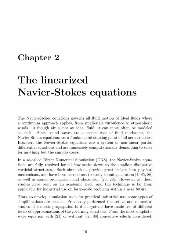
2.1 Derivation of the linearized Navier-Stokesequations

The full compressible Navier-Stokes equations are chosen as a starting point.These are derived from the assumptions on conservation of mass, momentumand energy and can be written in dimensional form as, [94]:

Continuity :Dρ

Dt+ ρ

∂uk∂xk

= 0

Momentum : ρDuiDt

= − ∂p

∂xi+∂τij∂xj

+ ρFi

Energy : ρDe

Dt= −p∂uk

∂xk+ Φ +

∂

∂xk

(κ∂T

∂xk

) (2.1)

with

Φ = τij∂ui∂xj

, τij = µ

(∂ui∂xj

+∂uj∂xi− 2

3∂uk∂xk

δij

)(2.2)

and e = e(p, T ), p = ρRT , where ρ is the density, p is the pressure, R isthe universal gas constant, T is the absolute temperature, ui is the velocitycomponent in the i:th direction, τij is the viscous stress tensor, Fi is a

18

volume force in the i:th direction, e is the internal energy, κ is the thermalconductivity, µ is the dynamic viscosity, Φ is the dissipation function, D/Dtis the convective derivative, δij is the Kronecker delta function, and theEinstein summation convention is used.

Due to the high computational demands associated with three-dimensionalsimulations, all simulations in this thesis are carried out in two dimensions.

We first assume that the solution can be written as a sum of a time-independent mean flow term and a time-dependent perturbation term:

ρ(x, t) = ρ0(x) + ρ′(x, t), u(x, t) = u0(x) + u′(x, t),v(x, t) = v0(x) + v′(x, t), p(x, t) = p0(x) + p′(x, t) (2.3)

where u = u1 and v = u2. We then introduce Eqs. (2.3) in Eqs. (2.1) andassume that quadratic and higher order perturbation terms are sufficientlysmall to be neglected.

Furthermore we assume that the relation between pressure and density can beregarded as isentropic. This is not applicable for all flows, e.g. combustion,but other studies indicate that this assumption is appropriate for types ofproblems similar to the ones treated in this thesis [59, 67, 93]. The assumptiondecreases the implementational and computational effort. In this case thepressure and density perturbations are related as [95]:

∂p′

∂xi= c2

∂ρ′

∂xi, (2.4)

where c2(x) = γp0/ρ0 is the local adiabatic speed of sound, and γ is theratio of specific heats. With this relation, the fluctuating pressure becomesredundant and can be removed from the system, and the continuity andmomentum equations are decoupled from the energy equation, which in turncan be omitted from the system of Equations (2.1). In this way, the size ofthe computational problem is considerably reduced.

A frequency domain approach is taken by prescribing harmonic time-dependence of the perturbed quantities. In this way, any perturbed quantityq′ can be represented as q′(x, t) = Re{q(x)e−iωt

}, where q is a complex

quantity and ω is the angular frequency. For implementational aspects werewrite the dimensional linearized Navier-Stokes equations on the form:

ρ :

(u0 v0)∇ρ+(∂u0

∂x+

∂v0

∂y− iω

)ρ = −

(∂ρ0u

∂x+∂ρ0v

∂y

)(2.5)

19

u :

∇T(−(

43µ 00 µ

)∇u)

+ ρ0(u0 v0)∇u+ ρ0

(∂u0

∂x− iω

)u =

= ρ0Fx −(u0∂u0

∂x+ v0

∂u0

∂y

)ρ− c2 ∂ρ

∂x+

13µ∂2v

∂x∂y− ρ0

∂u0

∂yv (2.6)

v :

∇T(−(µ 00 4

3µ

)∇v)

+ ρ0(u0 v0)∇v + ρ0

(∂v0

∂y− iω

)v =

= −c2 ∂ρ∂y−(u0∂v0

∂x+ v0

∂v0

∂y

)ρ− ρ0

∂v0

∂xu+

13µ∂2u

∂x∂y(2.7)

where ∇ = (∂/∂x ∂/∂y)T .

This formulation of the frequency-domain linearized Navier-Stokes equationswill be used in the first part of this thesis. In Chapter 4 it will however bereworked.

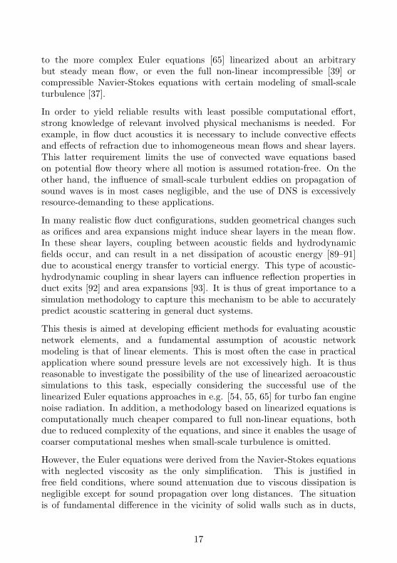
2.2 Boundary conditions

Along with the Eqs. (2.5-2.7), three different kinds of boundary conditionsare needed for the present work: slip and no-slip wall boundary conditionsand non-reflecting in-/outflow boundary conditions.

On the surfaces where acoustic boundary layers are assumed to have acertain level of influence, rigid wall no-slip boundary conditions are used,and implemented as

u = 0, n · ∇ρ = 0, (2.8)

where n is a unit vector normal to the walls. It should be noted that sincethe velocity components are restricted to zero on all sharp edges, no explicitKutta edge condition is needed when no-slip boundary conditions are used.

At the duct walls mainly governed by simple plane wave propagation, rigidwall slip boundary conditions,

u · n = 0, n · ∇ρ = 0, (2.9)

20

are used. The benefit of this choice is that the acoustic boundary layersalong the duct walls needs not to be resolved by the computational mesh,which in turn considerably decreases the computational effort. On the otherhand, this implies that the viscous dissipation associated with the dampingeffect at these walls are not included in the model governing equations. Inacoustically compact regions, this effect is negligible however, and for theevaluation of scattering at the duct element, this damping can be accountedfor by theoretical means if needed.

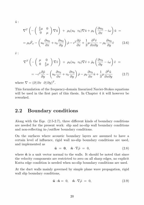
At the in- and outflow boundaries, only plane waves are assumed to bepresent, and thus non-reflecting boundary conditions based on the convectedHelmholtz equation,

n · ∇ρ = ikρ, n · ∇u = iku, v = 0, (2.10)

for a vertical boundary are employed. Here k is the wave number, andk = ω/(c − u0) at the upstream boundary and k = ω/(c + u0) at thedownstream boundary. These non-reflecting boundary conditions break downin the presence of vorticity, where the Helmholtz equation is not satisfied.Therefore, additional variable viscosity is applied in so-called buffer zones.This can be written as

µ = µphysical + µartificial (2.11)

where the artificial dynamic viscosity µartificial = 0 inside the physicaldomain and is then ramped up as a cubic polynomial through the buffer zoneto a specific value of, in this case, µartificial = 10 at the boundaries. Theefficiency of this strategy was investigated and found to yield low reflectionsof the order of less than 1% of the amplitudes of the acoustic waves. It washowever found to be less suitable for low frequencies when the computationaldomain was smaller than the acoustic wavelengths.

2.3 Forcing functions

As an acoustic source in Eq. (2.6), a time-harmonic body force function,F (x), was applied over a limited region in the domain. The advantage withemploying forcing functions inside a domain rather than in the boundaryconditions is that non-reflective boundary conditions can then be readilyapplied at the in- and outflow boundaries. The body force functions areimplemented as bell-shaped piece-wise cubic interpolation polynomials, as

21

Dirac pulses of Heaviside step functions were found to generate spuriousoscillations due to their discontinuous behavior. Suitable source regions werefound to be in the buffer zones, close to the physical domain.

2.4 Frequency scalings

Due to the two-dimensional approximation taken in the derivation ofthis implementation of the linearized Navier-Stokes equations, the cut-on frequency of the first higher order duct mode occur at a differentfrequency as compared to in a full three dimensional geometry. In thiswork, simulation results will be validated to experimental data acquired oncylindrical geometries, and according to [93, 96, 97], it is possible to introducea frequency scaling to enable a comparison of acoustic propagation in two andthree dimensions, the so-called normalized Helmholtz number, He∗. Thenormalized Helmholtz number is defined as the Helmholtz number dividedby the Helmholtz number of the cut-on frequency of the first higher-orderpropagating duct mode, i.e.

He∗ = He/Hecut-on. (2.12)

To relate the results of a two-dimensional model to those of the three-dimensional problem, the normalized Helmholtz number, He∗, of the twocases should be equal, such that He∗ = 1 at cut-on for both geometries.The Helmholtz numbers of a two dimensional duct and a cylindrical threedimensional duct can be defined as

He2D =2πf2D

cH, Hecyl =

2πfcyl

cA (2.13)

respectively. Here H is a relevant length scale in the two dimensional case,commonly the duct height, and A is a relevant length scale in the cylindricalthree dimensional case, often the duct radius. In case of symmetricalgeometries, only symmetric modes will be excited. Thus, the cut-onHelmholtz numbers are Hecut-on = 2π for the two dimensional geometry,and for the cylindrical duct Hecut-on = κ0 where κ0 ≈ 3.832 is the first zeroto the zeroth order Bessel function. This determines the relation between thefrequencies of the two-dimensional calculations and those of measurementsin a cylindrical duct.

22

2.5 The scattering matrix formalism

The acoustic network modeling can be formulated in various ways to representthe scattering of sound within each element. In the mobility matrix formalism[98], acoustic pressure at each port is used as input state variables and thecorresponding acoustic volume velocities are chosen as output states. Thiswas shown to yield the smallest possible number of unknowns, equal to thenumber of nodes. However, this assumes continuity of pressure and volumevelocity at the nodes, which is not a limitation in other methods.

The transfer matrix is an often used formalism [87, 99], especially suitable toduct configurations where elements are mounted in cascade (i.e. serial) andno sources are present within the duct system. Acoustic pressure and volumevelocity is used as state variables. Although implementationally straightforward in the cases of serial elements, it is less suited for more generalnetworks with arbitrary couplings [100].

The most general formulation is the scattering matrix approach [19] in whichthe number of unknowns equal 2M where M is the total number of elementsin the system. The scattering matrix formulation is derived to efficientlymodel networks with both serial and parallel element connections. Soundgeneration with elements is natively included. Often scattering matrices areobtained from analytical solutions or measurement data. Analytical solutionsare however often difficult to find, and measurements are expensive to carryout for a large number of components of varying geometrical parameters andflow speeds.

The aim of this thesis is to develop a fast and efficient yet physicallyrealistic simulation methodology such that the acoustical performance ofindividual network elements may be numerically predicted. Althoughdifferent implementationally and computationally, it can be shown that allnetwork representation formalisms can be transformed into each other. Thusthe choice of formalism for representation of the acoustic scattering is notrelevant to this thesis. However, since all experimental results used forbenchmarking are presented on the scattering matrix formalism, this is theformalism used throughout this thesis. In cases treated here, the elementsare assumed linear and time-invariant.

A general 2-port element can, in the frequency domain, be written as

23

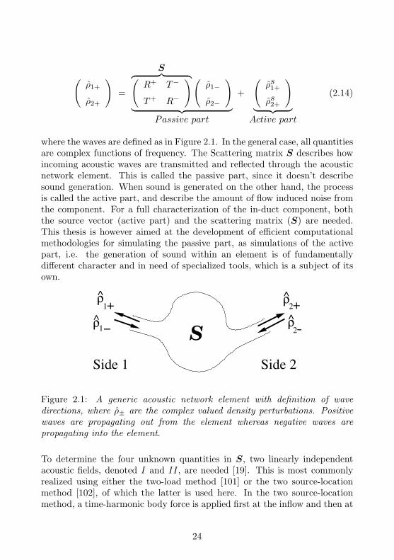
(ρ1+

ρ2+

)=

S︷︸︸︷(R+ T−

T+ R−

)(ρ1−

ρ2−

)︸︷︷︸

Passive part

+

(ρs1+

ρs2+

)︸︷︷︸Active part

(2.14)

where the waves are defined as in Figure 2.1. In the general case, all quantitiesare complex functions of frequency. The Scattering matrix S describes howincoming acoustic waves are transmitted and reflected through the acousticnetwork element. This is called the passive part, since it doesn’t describesound generation. When sound is generated on the other hand, the processis called the active part, and describe the amount of flow induced noise fromthe component. For a full characterization of the in-duct component, boththe source vector (active part) and the scattering matrix (S) are needed.This thesis is however aimed at the development of efficient computationalmethodologies for simulating the passive part, as simulations of the activepart, i.e. the generation of sound within an element is of fundamentallydifferent character and in need of specialized tools, which is a subject of itsown.

ρρ

ρ ρ

S

Side 1 Side 2

−

+

1

1

2−

2+

Figure 2.1: A generic acoustic network element with definition of wavedirections, where ρ± are the complex valued density perturbations. Positivewaves are propagating out from the element whereas negative waves arepropagating into the element.

To determine the four unknown quantities in S, two linearly independentacoustic fields, denoted I and II, are needed [19]. This is most commonlyrealized using either the two-load method [101] or the two source-locationmethod [102], of which the latter is used here. In the two source-locationmethod, a time-harmonic body force is applied first at the inflow and then at

24

the outflow to obtain two independent acoustic cases. The forcing functionsare described in Section 2.3. The scattering matrix can then be calculatedfrom

S =

[R+ T−

T+ R−

]=

[ρIa+ ρIIa+

ρIb+ ρIIb+

][ρIa− ρIIa−

ρIb− ρIIb−

]−1

(2.15)

where R+ and R− represents the upstream side and downstream side planewave reflection coefficients, respectively, and T+ and T− represents theupstream-to-downstream side and downstream-to-upstream side plane wavetransmission coefficients, respectively.

2.6 Plane wave decomposition methods

In order to characterize the acoustic scattering caused by the geometries, itis necessary to know the magnitudes and phases of the up- and downstreampropagating waves on both sides of the geometry, i.e. ρ± of Figure 2.1. Thedensity and velocity perturbations are given by Eqs. (2.5-2.7), which containboth acoustical and vortical contributions. Knowledge of ρ± is thus notreadily available, which calls for some postprocessing procedure. This is oftenreferred to as a plane wave decomposition of the perturbation field, since weonly study the scattering of plane waves. Several plane wave decompositionmethods has been proposed, as for example the the Two-Microphone Method[103], Full Wave Decomposition [104], or methods based on characteristicsbased filtering and Wiener-Hopf techniques [36, 105, 106].

2.6.1 Density-velocity method

To obtain the up- and downstream propagating acoustic waves from thesimulated solution, knowledge of plane wave propagation is utilized. It isassumed that the acoustic field quantities can be written as a sum of its up-and downstream propagating components, as

ρ = ρ+ + ρ−, u = u+ + u−. (2.16)

25

For a plane wave, the relation ρ = ±ρ0/c0u is valid, and thus, the wavedecomposition can be written as

ρ±(x) =12

(ρmean ± ρ0

c0umean

)(2.17)

where mean is an averaging of the quantities over the duct cross section, i.e.,

ρmean(x) =1H

H∫0

ρ(x, y)dy, (2.18)

where H in this case is the duct height either upstream or downstream ofthe duct element, and correspondingly for the velocity perturbations. Thisis the plane wave decomposition method used in Paper I in this thesis.

This approach is both simplistic and easily implemented. However, since itis based on plane wave relations between density and velocity perturbations,it is sensitive to disturbances due to numerical errors or vorticial motionwhere the plane wave assumption is not fulfilled. In addition, the methodonly yields information on the magnitudes of the propagating waves, and noinformation on their phase relations.

2.6.2 Curve-fitting method

To overcome the sensitivity to vorticial motion of previous method, and tobe able to extract phase information of the plane waves, a more sophisticatedplane wave decomposition method was implemented and used in Paper II.The method is based on a non-linear curve-fitting algorithm to the numericalsolutions of Eqs (2.5-2.7) to determine the magnitudes, phases and wavenumbers of the up- and downstream propagating waves, respectively. It isassumed that the acoustic field quantities can be written as a sum of up- anddownstream propagating plane waves, as

ρ = ρ+ + ρ−, u = u+ + u− (2.19)

All quantities are assumed averaged over the duct cross-section, in accordancewith Eq. (2.18). The acoustic particle velocity due to two up- anddownstream propagating plane waves can be written as

ρ(x) = |ρ+|eiφ+eik+x + |ρ−|eiφ−e−ik−x (2.20)

26

where |ρ±|, k± and φ± are real quantities representing the amplitudes,wave numbers and phases of the up- and downstream propagating waves,respectively. A plus sign denotes propagation in the positive x-direction,and a minus sign propagation in the negative x-direction. Since we haveimposed slip boundary conditions at the duct walls, no damping of the soundwaves due to visco-thermal losses at acoustic boundary layers are present,and damping due to bulk viscosity is considered negligible. Thus the wavenumbers can be assumed to be real.

Two postprocessing zones are chosen, upstreams and downstream of theacoustic network element under consideration. About hundred points in thex-direction is taken in each zones and used in an overdetermined non-linearleast-squares curve fitting to Eq. (2.20) to find the amplitudes and phasesof the up- and downstream propagating waves on both sides of the areaexpansion.

Any iterative non-linear least-squares curve-fitting algorithm needs an initialapproximation for the quantities to be solved for. For the wave numbers, therelation

k± =ω

c± u0(2.21)

is used, and for the magnitudes and phases, we use Eq. (2.20) and itsderivative

dρ(x)dx

= ik+|ρ+|eiφ+eik+x − ik−|ρ−|eiφ−e−ik−x (2.22)

combined with the estimated wavenumbers from Eq. (2.21). Initialapproximations of the magnitudes and phases are then found as

|ρ+|eiφ+ =e−ik+x

k+ + k−

(k−ρ(x) + i

dρ(x)dx

)(2.23)

|ρ−|eiφ− =eik+x

k+ + k−

(k+ρ(x)− idρ(x)

dx

). (2.24)

One downside of this wave decomposition technique is that Eq. (2.20) isno longer valid in the presence of vortical waves, as it is based on acousticwave propagation solely. If the evaluation zones are chosen sufficiently large,the acoustic waves and the vorticity waves will not be correlated in spaceover this region, and vorticity will not significantly affect the performance ofthe decomposition method. However, in the cases of low frequencies and at

27

high Mach numbers, the length scales of the vortical waves are larger, andmight be correlated over the evaluation zone, and will thus yield less accurateresults from the wave decomposition method.

Once the up- and downstream propagating waves on both sides of the areaexpansion are known, the scattering matrix can be calculated as describedby Eq. (2.15).

28

Chapter 3

Validation cases

In order to evaluate the proposed methodology from both a modeling as wellas computational point of view, investigations of the scattering of acousticplane waves in several duct configurations were carried out. The geometriesconsist of straight two-dimensional ducts with thin and thick orifice platesmounted inside, and of area expansions. The geometries were chosen toenable comparisons of the simulation results to experimental data [107–109]and analytical solutions [93, 96, 97, 110] of the various cases.

3.1 Thin orifice plate

The first validation case consists of a thin orifice plate mounted in a straightduct. This configuration is common in pipe systems for regulation of the flowlevel by varying the orifice area. As a side effect, the orifice plate configurationalso has a significant influence of the acoustical performance of the ductsystem.

3.1.1 Geometry

A schematic overview of the geometry in the calculation is shown inFigure 3.1. The duct length of the full experimental rig is around 7 m, buthere only a small section of less than 2 m is simulated to reduce computational

29

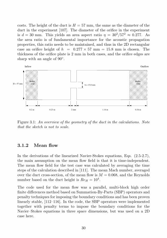
costs. The height of the duct is H = 57 mm, the same as the diameter of theduct in the experiment [107]. The diameter of the orifice in the experimentis d = 30 mm. This yields an area aspect ratio η = 302/572 ≈ 0.277. Asthe area ratio is of fundamental importance for the acoustic propagationproperties, this ratio needs to be maintained, and thus in the 2D rectangularcase an orifice height of h = 0.277 × 57 mm = 15.8 mm is chosen. Thethickness of the orifice plate is 2 mm in both cases, and the orifice edges aresharp with an angle of 90◦.

��

��

��

��

2 mm

Buffer

zone

Buffer

zone

0.2 m 0.23 m 1.14 m 0.34 m

h = 15.8 mmH = 57 mm

OutflowInflow

Figure 3.1: An overview of the geometry of the duct in the calculations. Notethat the sketch is not to scale.

3.1.2 Mean flow

In the derivations of the linearized Navier-Stokes equations, Eqs. (2.5-2.7),the main assumption on the mean flow field is that it is time-independent.The mean flow field for the test case was calculated by averaging the timesteps of the calculation described in [111]. The mean Mach number, averagedover the duct cross-section, of the mean flow is M = 0.068, and the Reynoldsnumber based on the duct height is ReH = 104.

The code used for the mean flow was a parallel, multi-block high orderfinite differences method based on Summation-By-Parts (SBP) operators andpenalty techniques for imposing the boundary conditions and has been provenlinearly stable, [112–116]. In the code, the SBP operators were implementedtogether with penalty terms to impose the boundary conditions for theNavier–Stokes equations in three space dimensions, but was used on a 2Dcase here.

30

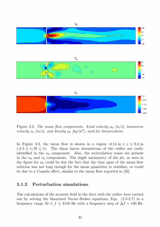
Figure 3.2: The mean flow components. Axial velocity u0 [m/s], transversevelocity v0 [m/s], and density ρ0 [kg/m3], used for linearization.

In Figure 3.2, the mean flow is shown in a region -0.14 m 6 x 6 0.3 m(-2.5 6 x/H 6 5). The shear layers downstream of the orifice are easilyidentified in the u0 component. Also, the recirculation zones are presentin the u0 and v0 components. The slight asymmetry of the jet, as seen inthe figure for u0 could be due the fact that the time span of the mean flowsolution was not long enough for the mean quantities to stabilize, or couldbe due to a Coanda effect, similar to the mean flow reported in [33].

3.1.3 Perturbation simulations

The calculations of the acoustic field in the duct with the orifice were carriedout by solving the linearized Navier-Stokes equations, Eqs. (2.5-2.7) in afrequency range 50 6 f 6 3150 Hz with a frequency step of ∆f = 100 Hz.

31

All frequencies are below the cut-on frequency of the first higher order mode,which in a circular duct with radius r = 2.85 mm and rigid walls is [117]:

f c =c0k1,0

2π

√1−M2 ≈ 3.5 kHz, (3.1)

where k1,0 ≈ 1.84/r.

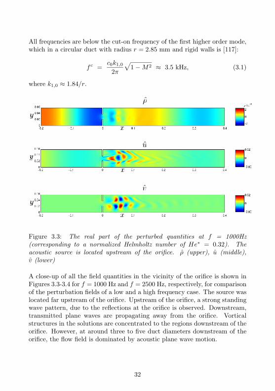
Figure 3.3: The real part of the perturbed quantities at f = 1000Hz(corresponding to a normalized Helmholtz number of He∗ = 0.32). Theacoustic source is located upstream of the orifice. ρ (upper), u (middle),v (lower)

A close-up of all the field quantities in the vicinity of the orifice is shown inFigures 3.3-3.4 for f = 1000 Hz and f = 2500 Hz, respectively, for comparisonof the perturbation fields of a low and a high frequency case. The source waslocated far upstream of the orifice. Upstream of the orifice, a strong standingwave pattern, due to the reflections at the orifice is observed. Downstream,transmitted plane waves are propagating away from the orifice. Vorticalstructures in the solutions are concentrated to the regions downstream of theorifice. However, at around three to five duct diameters downstream of theorifice, the flow field is dominated by acoustic plane wave motion.

32

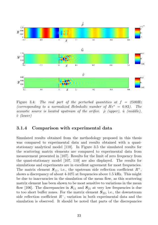
Figure 3.4: The real part of the perturbed quantities at f = 2500Hz(corresponding to a normalized Helmholtz number of He∗ = 0.83). Theacoustic source is located upstream of the orifice. ρ (upper), u (middle),v (lower)

3.1.4 Comparison with experimental data

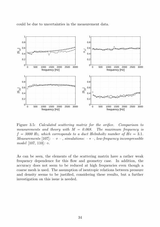
Simulated results obtained from the methodology proposed in this thesiswas compared to experimental data and results obtained with a quasi-stationary analytical model [110]. In Figure 3.5 the simulated results forthe scattering matrix elements are compared to experimental data frommeasurement presented in [107]. Results for the limit of zero frequency fromthe quasi-stationary model [107, 110] are also displayed. The results forsimulations and experiments are in excellent agreement for most frequencies.The matrix element S11, i.e., the upstream side reflection coefficient R+,shows a discrepancy of about 4-10% at frequencies above 1.5 kHz. This mightbe due to inaccuracies in the simulation of the mean flow, as this scatteringmatrix element has been shown to be most sensitive to variations in the meanflow [106]. The discrepancies in S11 and S21 at very low frequencies is dueto too short buffer zones. For the matrix element S22, i.e., the downstreamside reflection coefficient R−, variation in both experimental data and thesimulation is observed. It should be noted that parts of the discrepancies

33

could be due to uncertainties in the measurement data.

0 500 1000 1500 2000 2500 30000

0.2

0.4

0.6

0.8

1

frequency [Hz]

|S11

|

0 500 1000 1500 2000 2500 30000

0.2

0.4

0.6

0.8

1

frequency [Hz]

|S12

|

0 500 1000 1500 2000 2500 30000

0.2

0.4

0.6

0.8

1

frequency [Hz]

|S21

|

0 500 1000 1500 2000 2500 30000

0.2

0.4

0.6

0.8

1

frequency [Hz]

|S22

|

Figure 3.5: Calculated scattering matrix for the orifice. Comparison tomeasurements and theory with M = 0.068. The maximum frequency isf = 3000 Hz, which corresponds to a duct Helmholtz number of He = 3.1.Measurements [107]: – + – , simulations: – ∗ –, low-frequency incompressiblemodel [107, 110]: �.

As can be seen, the elements of the scattering matrix have a rather weakfrequency dependence for this flow and geometry case. In addition, theaccuracy does not seem to be reduced at high frequencies even though acoarse mesh is used. The assumption of isentropic relations between pressureand density seems to be justified, considering these results, but a furtherinvestigation on this issue is needed.

34

3.2 Area expansion

As a second validation case, the scattering of acoustic plane waves at aflow duct area expansion was considered. Several Mach number cases wereinvestigated, and both scattering matrices as well as end corrections werecalculated. Simulation results were compared to experimental data [108] andanalytical solutions [93, 96, 97].

3.2.1 Geometry

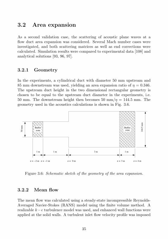
In the experiments, a cylindrical duct with diameter 50 mm upstream and85 mm downstream was used, yielding an area expansion ratio of η = 0.346.The upstream duct height in the two dimensional rectangular geometry ischosen to be equal to the upstream duct diameter in the experiments, i.e.50 mm. The downstream height then becomes 50 mm/η = 144.5 mm. Thegeometry used in the acoustics calculations is shown in Fig. 3.6.

��

��

��

��

Buffer

zone

Buffer

zone

1 m 3 m 1 m

144.5

mm

50 m

m

1 m

x =x =x = x = x =0 m−2 m −1 m 3 m 4 m

Figure 3.6: Schematic sketch of the geometry of the area expansion.

3.2.2 Mean flow

The mean flow was calculated using a steady-state incompressible Reynolds-Averaged Navier-Stokes (RANS) model using the finite volume method. Arealizable k−ε turbulence model was used, and enhanced wall functions wereapplied at the solid walls. A turbulent inlet flow velocity profile was imposed

35

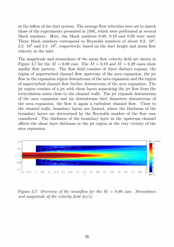
at the inflow of the duct system. The average flow velocities were set to matchthose of the experiments presented in [108], which were performed at severalMach numbers. Here, the Mach numbers 0.08, 0.19 and 0.29 were used.These Mach numbers correspond to Reynolds numbers of about 9.2 · 104,2.2 · 105 and 3.3 · 105, respectively, based on the duct height and mean flowvelocity at the inlet.

The magnitude and streamlines of the mean flow velocity field are shown inFigure 3.7 for the M = 0.08 case. The M = 0.19 and M = 0.29 cases showsimilar flow pattern. The flow field consists of three distinct regions; theregion of unperturbed channel flow upstream of the area expansion, the jetflow in the expansion region downstream of the area expansion and the regionof unperturbed channel flow further downstream of the area expansion. Thejet region consists of a jet with shear layers separating the jet flow from therecirculation zones close to the channel walls. The jet expands downstreamof the area expansion and six downstream duct diameters downstream ofthe area expansion, the flow is again a turbulent channel flow. Close tothe channel walls, boundary layers are formed, where the thickness of theboundary layers are determined by the Reynolds number of the flow caseconsidered. The thickness of the boundary layer in the upstream channelaffects the shear layer thickness in the jet region at the very vicinity of thearea expansion.

Figure 3.7: Overview of the meanflow for the M = 0.08 case. Streamlinesand magnitude of the velocity field [m/s].

36

3.2.3 Perturbation simulations

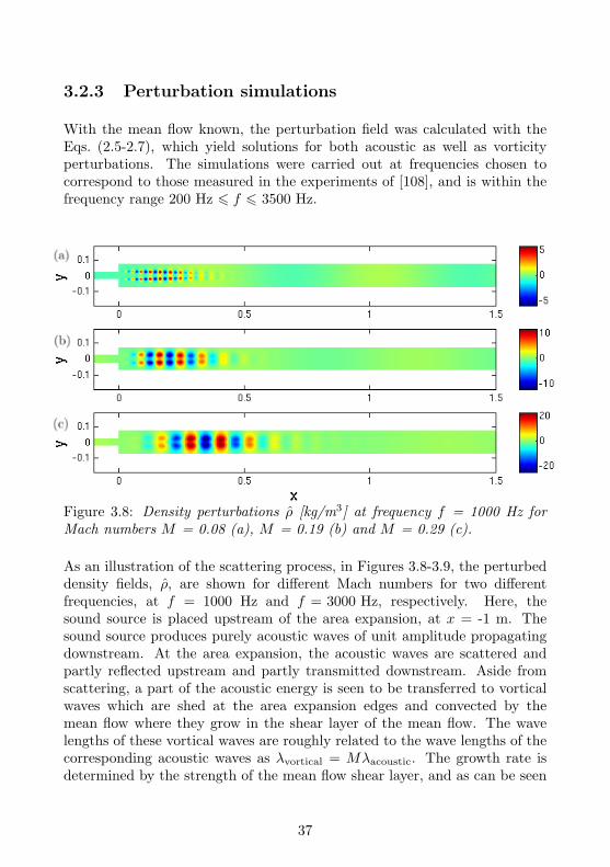
With the mean flow known, the perturbation field was calculated with theEqs. (2.5-2.7), which yield solutions for both acoustic as well as vorticityperturbations. The simulations were carried out at frequencies chosen tocorrespond to those measured in the experiments of [108], and is within thefrequency range 200 Hz 6 f 6 3500 Hz.

Figure 3.8: Density perturbations ρ [kg/m3] at frequency f = 1000 Hz forMach numbers M = 0.08 (a), M = 0.19 (b) and M = 0.29 (c).

As an illustration of the scattering process, in Figures 3.8-3.9, the perturbeddensity fields, ρ, are shown for different Mach numbers for two differentfrequencies, at f = 1000 Hz and f = 3000 Hz, respectively. Here, thesound source is placed upstream of the area expansion, at x = -1 m. Thesound source produces purely acoustic waves of unit amplitude propagatingdownstream. At the area expansion, the acoustic waves are scattered andpartly reflected upstream and partly transmitted downstream. Aside fromscattering, a part of the acoustic energy is seen to be transferred to vorticalwaves which are shed at the area expansion edges and convected by themean flow where they grow in the shear layer of the mean flow. The wavelengths of these vortical waves are roughly related to the wave lengths of thecorresponding acoustic waves as λvortical = Mλacoustic. The growth rate isdetermined by the strength of the mean flow shear layer, and as can be seen

37

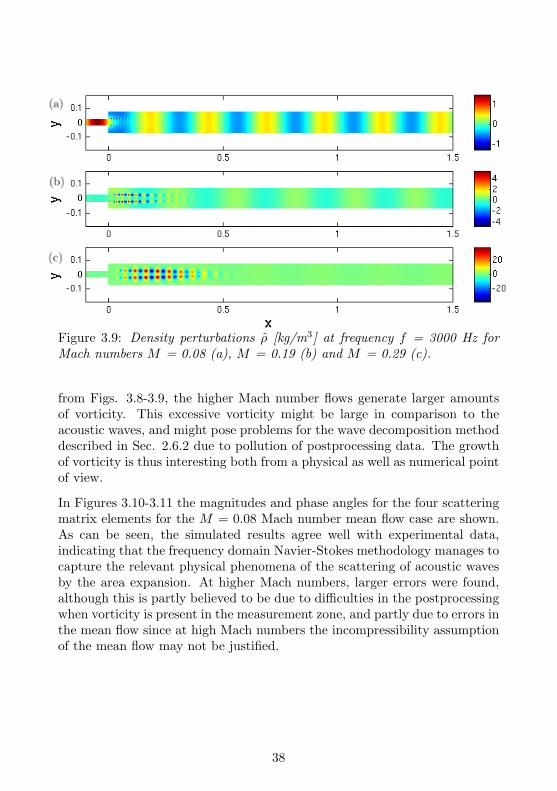
Figure 3.9: Density perturbations ρ [kg/m3] at frequency f = 3000 Hz forMach numbers M = 0.08 (a), M = 0.19 (b) and M = 0.29 (c).

from Figs. 3.8-3.9, the higher Mach number flows generate larger amountsof vorticity. This excessive vorticity might be large in comparison to theacoustic waves, and might pose problems for the wave decomposition methoddescribed in Sec. 2.6.2 due to pollution of postprocessing data. The growthof vorticity is thus interesting both from a physical as well as numerical pointof view.

In Figures 3.10-3.11 the magnitudes and phase angles for the four scatteringmatrix elements for the M = 0.08 Mach number mean flow case are shown.As can be seen, the simulated results agree well with experimental data,indicating that the frequency domain Navier-Stokes methodology manages tocapture the relevant physical phenomena of the scattering of acoustic wavesby the area expansion. At higher Mach numbers, larger errors were found,although this is partly believed to be due to difficulties in the postprocessingwhen vorticity is present in the measurement zone, and partly due to errors inthe mean flow since at high Mach numbers the incompressibility assumptionof the mean flow may not be justified.

38

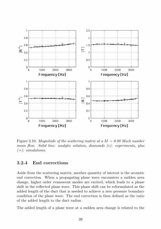
Figure 3.10: Magnitude of the scattering matrix at a M = 0.08 Mach numbermean flow. Solid line: analytic solution, diamonds (�): experiments, plus(+): simulations.

3.2.4 End corrections

Aside from the scattering matrix, another quantity of interest is the acousticend correction. When a propagating plane wave encounters a sudden areachange, higher order evanescent modes are excited, which leads to a phaseshift in the reflected plane wave. This phase shift can be reformulated as theadded length of the duct that is needed to achieve a zero pressure boundarycondition of the plane wave. The end correction is then defined as the ratioof the added length to the duct radius.

The added length of a plane wave at a sudden area change is related to the

39

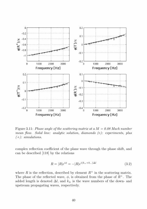
Figure 3.11: Phase angle of the scattering matrix at a M = 0.08 Mach numbermean flow. Solid line: analytic solution, diamonds (�): experiments, plus(+): simulations.

complex reflection coefficient of the plane wave through the phase shift, andcan be described [118] by the relations

R = |R|eiφ = −|R|ei(k++k−)∆l (3.2)

where R is the reflection, described by element R+ in the scattering matrix.The phase of the reflected wave, φ, is obtained from the phase of R+. Theadded length is denoted ∆l, and k± is the wave numbers of the down- andupstream propagating waves, respectively.

40

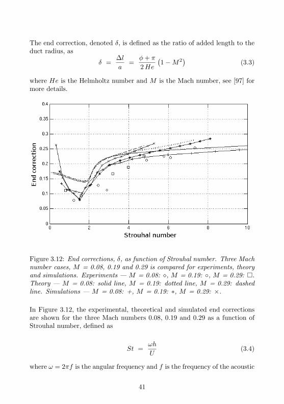
The end correction, denoted δ, is defined as the ratio of added length to theduct radius, as

δ =∆la

=φ+ π

2He(1−M2

)(3.3)

where He is the Helmholtz number and M is the Mach number, see [97] formore details.

Figure 3.12: End corrections, δ, as function of Strouhal number. Three Machnumber cases, M = 0.08, 0.19 and 0.29 is compared for experiments, theoryand simulations. Experiments — M = 0.08: �, M = 0.19: ◦, M = 0.29: �.Theory — M = 0.08: solid line, M = 0.19: dotted line, M = 0.29: dashedline. Simulations — M = 0.08: +, M = 0.19: ∗, M = 0.29: ×.

In Figure 3.12, the experimental, theoretical and simulated end correctionsare shown for the three Mach numbers 0.08, 0.19 and 0.29 as a function ofStrouhal number, defined as

St =ωh

U(3.4)

where ω = 2πf is the angular frequency and f is the frequency of the acoustic

41

wave, h the height of the upstream duct section and U is the mean flowvelocity in the upstream duct section.

Firstly, it can be concluded that the frequency domain linearized Navier-Stokes equations with realistic mean flow profile manages to accuratelypredict the characteristics of the end correction, compared to experimentaldata. Furthermore, it is clearly seen that the end corrections collapsewhen displayed as function of Strouhal number, especially in the range1 < St < 2. This is due to the fact that this is the primary region of acoustic-hydrodynamic coupling. The acoustic response of the area expansion canbe divided into three regions, where St � 1, St ∼ O(1) or St � 1,governed by different mechanisms. These mechanisms are influenced byquasi-steady hydrodynamic flow, flow-acoustic interaction with excitation ofhydrodynamic waves, i.e. vortex shedding, and acoustic propagation withlittle effect of flow-acoustic interaction, respectively.

3.3 Whistling

A critical issue in flow duct configurations is the potential risk of flow-acoustic coupling leading to whistling, which counteracts the performanceof installed mufflers, and must be avoided. Although whistling itself is anon-linear phenomena, the onset from a linear state is not, and can thereforebe simulated with linear aeroacoustics. By calculating a so-called powerbalance over an individual duct component it can be seen that for certainconfigurations, for certain frequency ranges, more acoustical power is emittedthan put into the system. This is due to an interaction between the acousticaland the vorticial modes in the fluid, where an amount of acoustical power istransferred into vorticity which may be amplified in mean flow shear layers,and if interacting with for example an edge, emits more acoustic energy thanthat which to start with triggered the vorticity instability. In that case a netpower amplification can be caused. If this acoustic power amplification occursin a frequency range corresponding to any acoustical resonance frequenciesof the system, it may lead to a resonant feedback loop yielding very largeamplitudes such that transition from the linear state into a non-linear regimeoccurs.

The net attenuation or amplification of sound waves in a duct element ischaracterized by its scattering properties. From the scattering properties, theacoustical power output to a unit acoustical power input can be calculated[109, 119]. Frequency ranges with a net power amplification are identified as

42

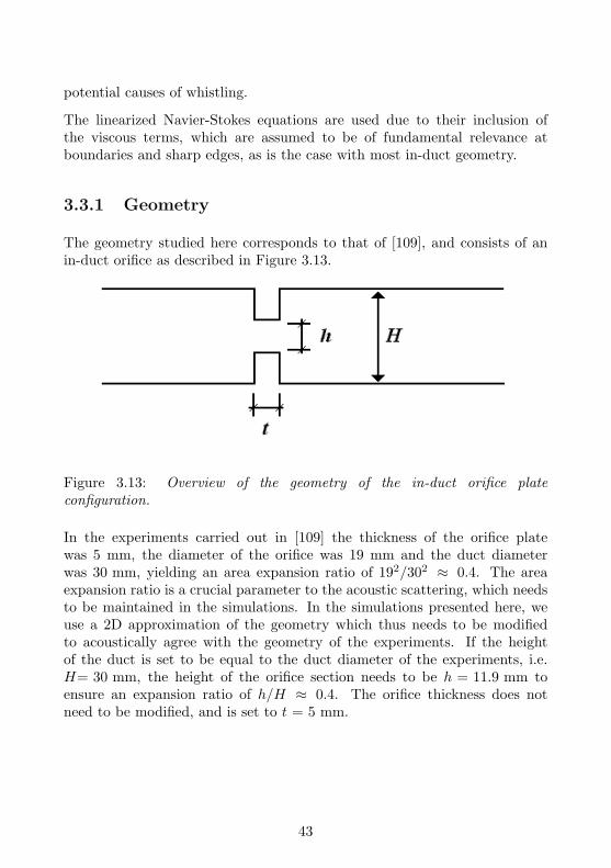
potential causes of whistling.

The linearized Navier-Stokes equations are used due to their inclusion ofthe viscous terms, which are assumed to be of fundamental relevance atboundaries and sharp edges, as is the case with most in-duct geometry.

3.3.1 Geometry

The geometry studied here corresponds to that of [109], and consists of anin-duct orifice as described in Figure 3.13.

Figure 3.13: Overview of the geometry of the in-duct orifice plateconfiguration.

In the experiments carried out in [109] the thickness of the orifice platewas 5 mm, the diameter of the orifice was 19 mm and the duct diameterwas 30 mm, yielding an area expansion ratio of 192/302 ≈ 0.4. The areaexpansion ratio is a crucial parameter to the acoustic scattering, which needsto be maintained in the simulations. In the simulations presented here, weuse a 2D approximation of the geometry which thus needs to be modifiedto acoustically agree with the geometry of the experiments. If the heightof the duct is set to be equal to the duct diameter of the experiments, i.e.H= 30 mm, the height of the orifice section needs to be h = 11.9 mm toensure an expansion ratio of h/H ≈ 0.4. The orifice thickness does notneed to be modified, and is set to t = 5 mm.

43

3.3.2 Mean flow

The first step in the simulation methodology is to calculate the mean flow inthe duct section, which later is used to linearize around. The flow is simulatedwith an incompressible, non-linear, steady-state Reynolds-Averaged Navier-Stokes (RANS) method, with a k − ε turbulence model.

Figure 3.14: Magnitude of the velocity field [m/s] and streamlines of thesteady-state mean flow.

The inflow Mach number is M = 0.042, which corresponds to a Reynoldsnumber ReH ≈ 2.5 · 104 based on the duct height. The magnitude of thevelocity of the mean flow field is shown in Figure 3.14 and is seen to bedominated by the formation of a jet with a maximum flow speed of M = 0.14in the region at the orifice, expanding further downstream and develops intochannel flow within 3-5 duct diameters. A large recirculation zone is alsoseen, with reattachment point at about 1.5 duct diameters downstream ofthe orifice plate. A close-up of the mean flow in the vicinity of the lowerorifice edge is shown in Figure 3.15, which reveals the formation of a smallerrecirculation zone just downstream of the leading edge of the orifice plate.

It should be pointed out that the recirculation zone within the cavity seemedto be sensitive to properties of the RANS modeling and computational meshused. As this recirculation zone influence the acoustic scattering, care shouldbe taken when calculating the mean flow.

44

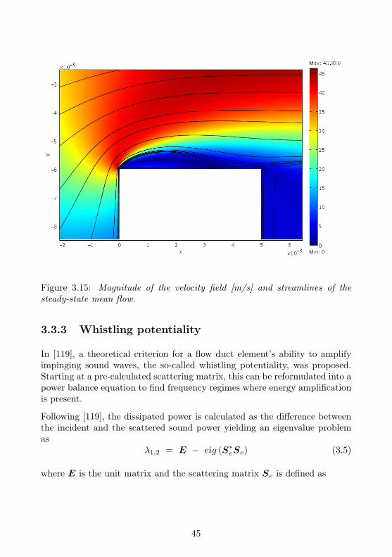
Figure 3.15: Magnitude of the velocity field [m/s] and streamlines of thesteady-state mean flow.

3.3.3 Whistling potentiality

In [119], a theoretical criterion for a flow duct element’s ability to amplifyimpinging sound waves, the so-called whistling potentiality, was proposed.Starting at a pre-calculated scattering matrix, this can be reformulated into apower balance equation to find frequency regimes where energy amplificationis present.

Following [119], the dissipated power is calculated as the difference betweenthe incident and the scattered sound power yielding an eigenvalue problemas

λ1,2 = E − eig (S∗eSe) (3.5)

where E is the unit matrix and the scattering matrix Se is defined as

45

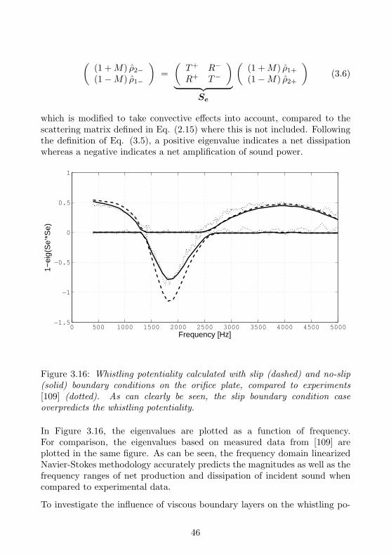
((1 +M) ρ2−(1−M) ρ1−

)=(T+ R−

R+ T−

)︸︷︷︸

Se

((1 +M) ρ1+

(1−M) ρ2+

)(3.6)

which is modified to take convective effects into account, compared to thescattering matrix defined in Eq. (2.15) where this is not included. Followingthe definition of Eq. (3.5), a positive eigenvalue indicates a net dissipationwhereas a negative indicates a net amplification of sound power.

0 500 1000 1500 2000 2500 3000 3500 4000 4500 5000−1.5

−1

−0.5

0

0.5

1

Frequency [Hz]

1−ei

g(S

e’*S

e)

Figure 3.16: Whistling potentiality calculated with slip (dashed) and no-slip(solid) boundary conditions on the orifice plate, compared to experiments[109] (dotted). As can clearly be seen, the slip boundary condition caseoverpredicts the whistling potentiality.

In Figure 3.16, the eigenvalues are plotted as a function of frequency.For comparison, the eigenvalues based on measured data from [109] areplotted in the same figure. As can be seen, the frequency domain linearizedNavier-Stokes methodology accurately predicts the magnitudes as well as thefrequency ranges of net production and dissipation of incident sound whencompared to experimental data.

To investigate the influence of viscous boundary layers on the whistling po-

46

tentiality, a second simulation was carried out with slip boundary conditionson the orifice plate, mimicking the behavior of a Linearized Euler Equations(LEE) simulation. The results are included in Figure 3.16 as well, showingan overprediction of whistling potentiality due to an increased vorticialstrength in the absence of boundary layers. This clearly demonstrates thata methodology based on LEE would be insufficient for this application.

3.3.4 Nyquist stability criterion

A constructed experimental set-up was arranged to produce whistling. Anorifice plate was placed in a duct of finite length, thus creating reflectionsfrom the duct ends back into the system. With large enough reflections andnegative whistling potentiality at a resonance frequency of the duct, whistlingmight occur if the acoustic amplification due to the orifice is larger than thedissipation in the system. The system was built modular to enable the up-and downstream duct lengths to be varied. Cases of a short duct of totallength of 0.8 m was investigated with the orifice placed at (A) 0.33 m fromthe inlet, and (B) 0.27 m from the inlet.

However, the whistling potentiality does not by itself determine whether aduct component give rise to whistling or not. This depends on the ductsystem as a whole and is influenced by the reflections at the duct system’sends back to the sound amplifying region. Therefore a description of thesystem as a whole is needed.

Let x− represent the acoustic waves propagating into the orifice plate fromthe duct endings. These waves are related to the acoustic waves propagatingoutwards from the orifice plate, denoted x+, as x− = Rx+, where R is thereflection coefficients of the duct ends, defined as

R =

ρ1−ρ1+

0

0 ρ2−ρ2+

(3.7)

With the use of the definition of the scattering matrix, x+ = Sx−, the totalpropagation system can be formulated as x+ = SRx+, or equivalently

(E − SR) x+ = 0 (3.8)

where E is the unit matrix. Non-trivial solutions (eigenfrequecies) exist when

Z(ω) ≡ det(E − SR) = 0 (3.9)

47

To identify the zeros of Z(ω), several methods can be used. One approachwhen data for Z is only available for positive and real frequencies, as is thecases when the system has been characterized numerically or experimentally,is to use the Nyquist stability criterion. The Nyquist method has previouslybeen applied to acoustics in [120, 121], to identify critical zeros associatedwith instabilities that may cause whistling. If the contour of Z(ω) is plottedin the complex plane, the number of critical zeros can be identified as thenumber of times the contour encircles the origin. The frequencies of theeigenmodes are found when Z(ω) cross the real axis on the negative side.

0 0.5 1 1.5 2

−1

−0.8

−0.6

−0.4

−0.2

0

0.2

0.4

0.6

0.8

1

Re{Z( ω)}

Im{Z

(ω

)}

0 0.5 1 1.5 2

−1

−0.8

−0.6

−0.4

−0.2

0

0.2

0.4

0.6

0.8

1

Re{Z( ω)}

(a) (b)

Figure 3.17: Nyquist plot of (a) Case A, and (b) Case B. Plus signs denotelow frequency start point and circles denote high frequency end points. Ascan be seen, the origin is encircled in Case A, indicating a whistling system.Case B does not encircle the origin and should thus not be prone to whistle.

The Nyquist analysis was based on the simulated scattering matrix. Theupstream reflection coefficient was measured and for the downstream outletthe theory of [92] was used to find the reflection coefficient. This yieldsa complete description of the duct system according to Eq. (3.9). InFigure 3.17, Z(ω) is presented in a Nyquist plot to predict the differentcases’ ability to whistle or not. As can be seen, Case A is predicted towhistle, whereas Case B is predicted to not whistle. The predicted whistlingfrequency of Case A is found where Z(ω) cross the real axis on the negativeside of the origin. In this case this occurs at a Strouhal number of 0.27.

To validate the predicted whistling of the duct system, experiments werecarried out where the sound pressure levels produced by the different cases

48

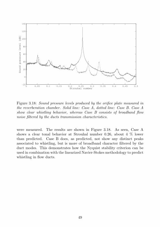
0 0.05 0.1 0.15 0.2 0.25 0.3 0.35 0.4 0.45 0.5−20

0

20

40

60

80

100

120

140

Strouhal number

So

un

d p

ress

ure

leve

l [d

B]

Figure 3.18: Sound pressure levels produced by the orifice plate measured inthe reverberation chamber. Solid line: Case A, dotted line: Case B. Case Ashow clear whistling behavior, whereas Case B consists of broadband flownoise filtered by the ducts transmission characteristics.

were measured. The results are shown in Figure 3.18. As seen, Case Ashows a clear tonal behavior at Strouhal number 0.26, about 4 % lowerthan predicted. Case B does, as predicted, not show any distinct peaksassociated to whistling, but is more of broadband character filtered by theduct modes. This demonstrates how the Nyquist stability criterion can beused in combination with the linearized Navier-Stokes methodology to predictwhistling in flow ducts.

49

Chapter 4

Global modes

In the previous chapter, the linearized Navier-Stokes equations were solveddirectly to obtain the scattering of sound. Here, another approach willbe taken, and the linearized Navier-Stokes equations will be solved as aneigenvalue problem. This is analogous to the Helmholtz equation which alsocan be solved both directly or as an eigenvalue problem, depending on typeof analysis needed.

The dynamics of a flow can be described in terms of its eigenmodes, the so-called global modes. This has successfully been used for stability analysis andflow control purposes, see for example [78, 122–127]. Although the theory hasbeen known for a long time, it is only in recent years that calculations havebeen possible to carry out in two or three space dimensions, due to increasingcomputational performance. Here the use of global modes for aeroacousticpurposes is evaluated.

Since every global mode is periodic in time, with the frequency determinedby its eigenvalue, it is possible to relate every frequency in a spectrum ofa generated sound to a specific global mode. Thus, the decomposition ofa flow field into its global mode enables the study of flow structures ofdifferent sound generating mechanisms isolated from each other. This is amethodological advantage over the use of DNS for aeroacoustic, since in DNSall source mechanisms are present at the same time and not easily isolatedfrom each other. However, the flow field needs to be within the linear regime,which limits the range of industrial applications of the methodology.

50

4.1 A reduced model of the flow field

The global modes are calculated by reformulating the linearized Navier-Stokes equations to an eigenvalue problem. We consider a two-dimensional,incompressible steady state base flow, but the methodology is applicable tomore general flows.

With a base flow U(x, y) = (U(x, y), V (x, y) ) and P (x, y), the Navier-Stokesequations for a small time-harmonic perturbation q = (u, v, p)T can beformulated as

−iωBq = Aq, (4.1)

where

A =

−U · ∇ − ∂U

∂x+

1Re∇2 −∂U

∂y− ∂

∂x

−∂V∂x

−U · ∇ − ∂V

∂y+

1Re∇2 − ∂

∂y

∂

∂x

∂

∂y0

(4.2)

and B = diag(1 1 0). This can be solved as an eigenvalue problem, andthus it is possible to find a set of eigenmodes such that the time-domainperturbations q can be written as

q(x, y, t) =N∑n=1

cn qn(x, y) e−iωnt (4.3)

where cn are constants determined by the initial condition. The eigenmodes,qn(x, y), are referred to as global modes since they are global in the sensethat they depend on all space dimensions. In a reduced model only a smallfraction N of the available global modes are used.

The benefit of writing the flow field on this form is that it is now possible tostudy the eigenmodes separately, or to analyze how different combinations ofeigenmodes interact. From a computational point of view this form is alsobeneficial since only a set of eigenmodes are required to be saved as oppositeto the whole flow field for every time step of a DNS solution.

51

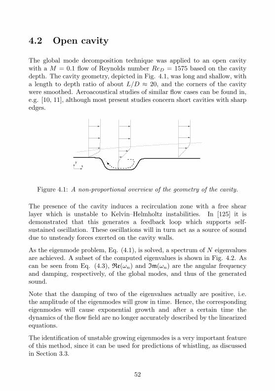
4.2 Open cavity

The global mode decomposition technique was applied to an open cavitywith a M = 0.1 flow of Reynolds number ReD = 1575 based on the cavitydepth. The cavity geometry, depicted in Fig. 4.1, was long and shallow, witha length to depth ratio of about L/D ≈ 20, and the corners of the cavitywere smoothed. Aeroacoustical studies of similar flow cases can be found in,e.g. [10, 11], although most present studies concern short cavities with sharpedges.

xy

Figure 4.1: A non-proportional overview of the geometry of the cavity.

The presence of the cavity induces a recirculation zone with a free shearlayer which is unstable to Kelvin–Helmholtz instabilities. In [125] it isdemonstrated that this generates a feedback loop which supports self-sustained oscillation. These oscillations will in turn act as a source of sounddue to unsteady forces exerted on the cavity walls.

As the eigenmode problem, Eq. (4.1), is solved, a spectrum of N eigenvaluesare achieved. A subset of the computed eigenvalues is shown in Fig. 4.2. Ascan be seen from Eq. (4.3), Re(ωn) and Im(ωn) are the angular frequencyand damping, respectively, of the global modes, and thus of the generatedsound.

Note that the damping of two of the eigenvalues actually are positive, i.e.the amplitude of the eigenmodes will grow in time. Hence, the correspondingeigenmodes will cause exponential growth and after a certain time thedynamics of the flow field are no longer accurately described by the linearizedequations.

The identification of unstable growing eigenmodes is a very important featureof this method, since it can be used for predictions of whistling, as discussedin Section 3.3.

52

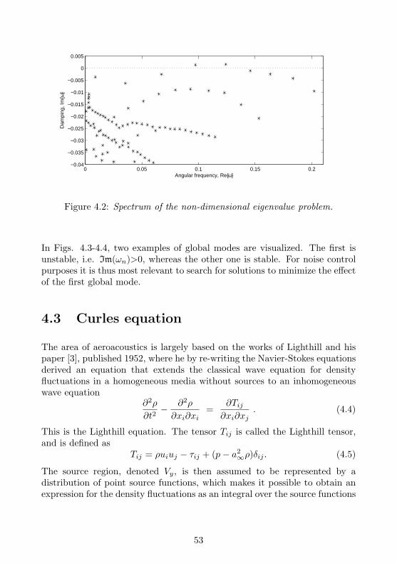
0 0.05 0.1 0.15 0.2−0.04

−0.035

−0.03

−0.025

−0.02

−0.015

−0.01

−0.005

0

0.005

Angular frequency, Re{ω}

Dam

ping

, Im

{ω}

Figure 4.2: Spectrum of the non-dimensional eigenvalue problem.

In Figs. 4.3-4.4, two examples of global modes are visualized. The first isunstable, i.e. Im(ωn)>0, whereas the other one is stable. For noise controlpurposes it is thus most relevant to search for solutions to minimize the effectof the first global mode.

4.3 Curles equation

The area of aeroacoustics is largely based on the works of Lighthill and hispaper [3], published 1952, where he by re-writing the Navier-Stokes equationsderived an equation that extends the classical wave equation for densityfluctuations in a homogeneous media without sources to an inhomogeneouswave equation

∂2ρ

∂t2− ∂2ρ

∂xi∂xi=

∂Tij∂xi∂xj

. (4.4)

This is the Lighthill equation. The tensor Tij is called the Lighthill tensor,and is defined as

Tij = ρuiuj − τij + (p− a2∞ρ)δij . (4.5)

The source region, denoted Vy, is then assumed to be represented by adistribution of point source functions, which makes it possible to obtain anexpression for the density fluctuations as an integral over the source functions

53

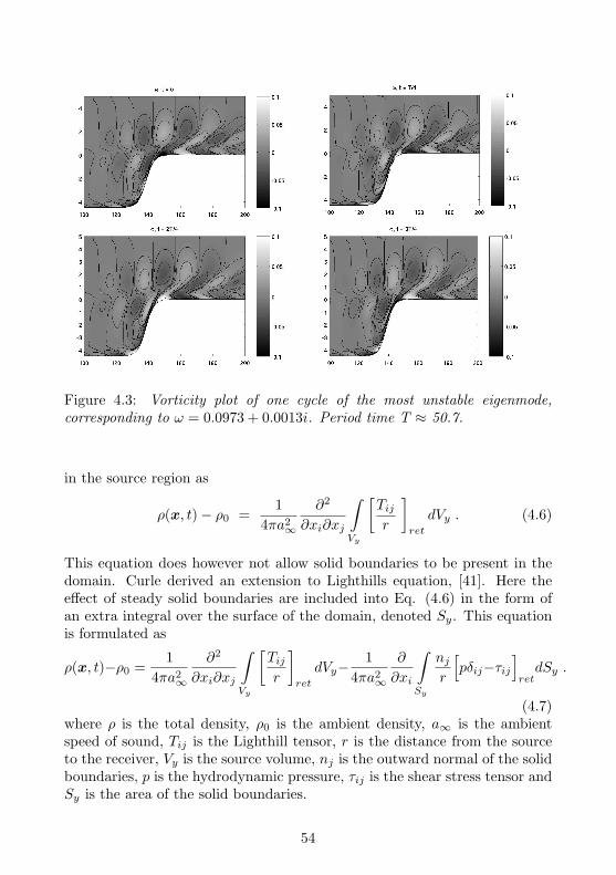
Figure 4.3: Vorticity plot of one cycle of the most unstable eigenmode,corresponding to ω = 0.0973 + 0.0013i. Period time T ≈ 50.7.

in the source region as

ρ(x, t)− ρ0 =1

4πa2∞

∂2

∂xi∂xj

∫Vy

[Tijr

]ret

dVy . (4.6)

This equation does however not allow solid boundaries to be present in thedomain. Curle derived an extension to Lighthills equation, [41]. Here theeffect of steady solid boundaries are included into Eq. (4.6) in the form ofan extra integral over the surface of the domain, denoted Sy. This equationis formulated as

ρ(x, t)−ρ0 =1

4πa2∞

∂2

∂xi∂xj

∫Vy

[Tijr

]ret

dVy− 14πa2∞

∂

∂xi

∫Sy

njr

[pδij−τij

]retdSy .

(4.7)where ρ is the total density, ρ0 is the ambient density, a∞ is the ambientspeed of sound, Tij is the Lighthill tensor, r is the distance from the sourceto the receiver, Vy is the source volume, nj is the outward normal of the solidboundaries, p is the hydrodynamic pressure, τij is the shear stress tensor andSy is the area of the solid boundaries.

54

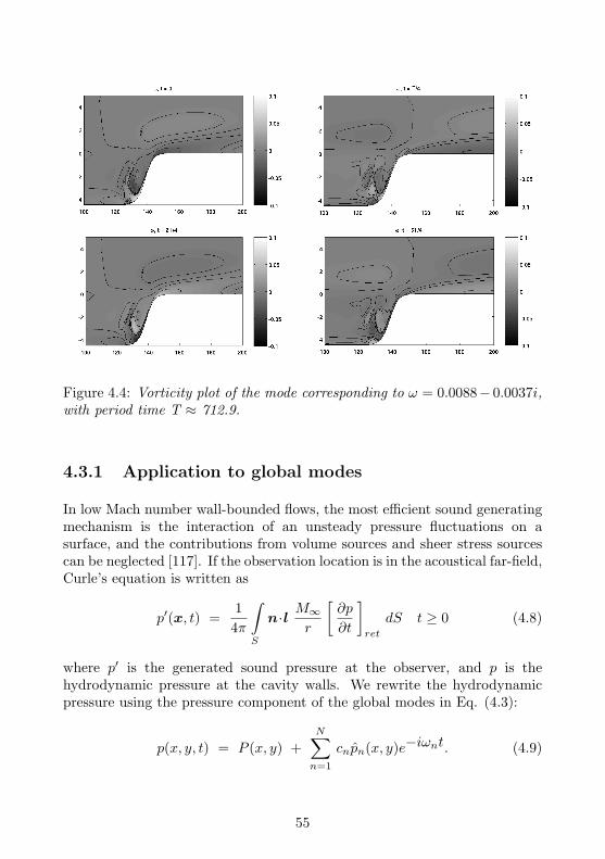
Figure 4.4: Vorticity plot of the mode corresponding to ω = 0.0088− 0.0037i,with period time T ≈ 712.9.

4.3.1 Application to global modes

In low Mach number wall-bounded flows, the most efficient sound generatingmechanism is the interaction of an unsteady pressure fluctuations on asurface, and the contributions from volume sources and sheer stress sourcescan be neglected [117]. If the observation location is in the acoustical far-field,Curle’s equation is written as

p′(x, t) =1

4π

∫S

n·l M∞r

[∂p

∂t

]ret

dS t ≥ 0 (4.8)

where p′ is the generated sound pressure at the observer, and p is thehydrodynamic pressure at the cavity walls. We rewrite the hydrodynamicpressure using the pressure component of the global modes in Eq. (4.3):

p(x, y, t) = P (x, y) +N∑n=1

cnpn(x, y)e−iωnt. (4.9)

55

and introduce Eq. (4.9) into Eq. (4.8). This yields

p′(x, t) =1

4π

∫S

n·l M∞r

∂

∂t

(P +

N∑n=1

cnpne−iωnτ

)dS .

The temporal derivative is equivalent to a multiplication with −iωn due tothe ansatz of harmonic time dependence, and the time independence of thebase pressure, hence

p′(x, t) =1

4π

∫S

n·l M∞r

N∑n=1

cnpn(− iωn)e−iωnτ dS .

which can be reformulated as

p′(x, t) =N∑n=1

cne−iωnt

− 14π

∫S

n·l M∞r

pniωneiωnM∞r dS

︸︷︷︸

≡ φn

. (4.10)

for t > M∞rmax where rmax is the distance from the observer to the pointin the source region that is furthest away from the observer location.

Note that φn is independent of time. This means that the integrals of φnonly needs to be calculated once for every global mode and every observationlocation. We have

p′(x, t) =N∑n=1

cnφn e−iωnt, t >M∞rmax. (4.11)

Writing Eq. (4.8) in the form of Eq. (4.11) is beneficial, since it makes it anextremely fast task to perform an analysis of a chosen initial condition. Also,since the equation is written as a sum of constant coefficients and complexexponential functions, the spectrum of the sound is in fact determined at thesame time as the sound itself.

56

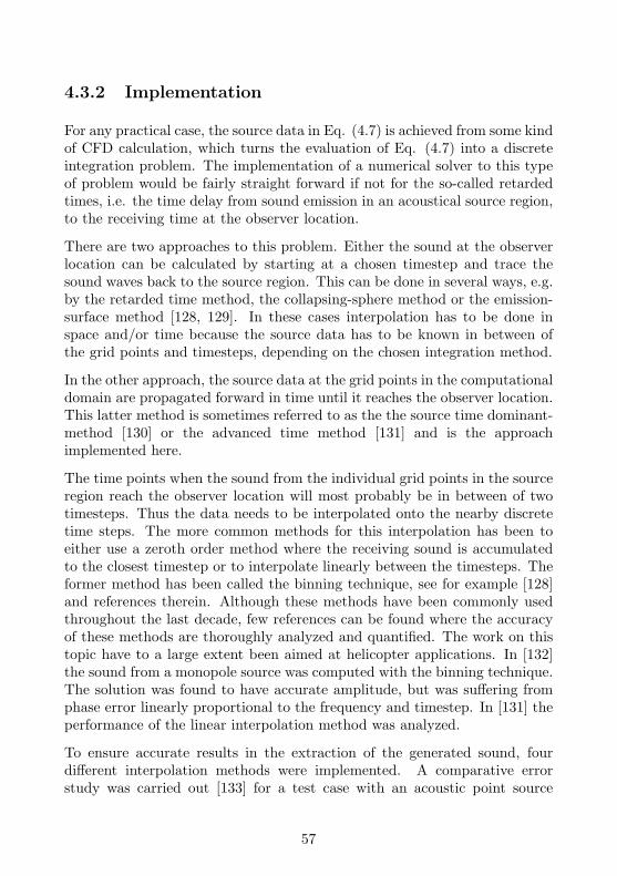
4.3.2 Implementation

For any practical case, the source data in Eq. (4.7) is achieved from some kindof CFD calculation, which turns the evaluation of Eq. (4.7) into a discreteintegration problem. The implementation of a numerical solver to this typeof problem would be fairly straight forward if not for the so-called retardedtimes, i.e. the time delay from sound emission in an acoustical source region,to the receiving time at the observer location.

There are two approaches to this problem. Either the sound at the observerlocation can be calculated by starting at a chosen timestep and trace thesound waves back to the source region. This can be done in several ways, e.g.by the retarded time method, the collapsing-sphere method or the emission-surface method [128, 129]. In these cases interpolation has to be done inspace and/or time because the source data has to be known in between ofthe grid points and timesteps, depending on the chosen integration method.

In the other approach, the source data at the grid points in the computationaldomain are propagated forward in time until it reaches the observer location.This latter method is sometimes referred to as the the source time dominant-method [130] or the advanced time method [131] and is the approachimplemented here.

The time points when the sound from the individual grid points in the sourceregion reach the observer location will most probably be in between of twotimesteps. Thus the data needs to be interpolated onto the nearby discretetime steps. The more common methods for this interpolation has been toeither use a zeroth order method where the receiving sound is accumulatedto the closest timestep or to interpolate linearly between the timesteps. Theformer method has been called the binning technique, see for example [128]and references therein. Although these methods have been commonly usedthroughout the last decade, few references can be found where the accuracyof these methods are thoroughly analyzed and quantified. The work on thistopic have to a large extent been aimed at helicopter applications. In [132]the sound from a monopole source was computed with the binning technique.The solution was found to have accurate amplitude, but was suffering fromphase error linearly proportional to the frequency and timestep. In [131] theperformance of the linear interpolation method was analyzed.

To ensure accurate results in the extraction of the generated sound, fourdifferent interpolation methods were implemented. A comparative errorstudy was carried out [133] for a test case with an acoustic point source

57

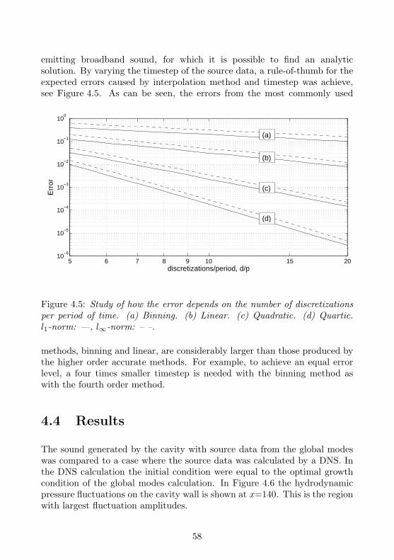
emitting broadband sound, for which it is possible to find an analyticsolution. By varying the timestep of the source data, a rule-of-thumb for theexpected errors caused by interpolation method and timestep was achieve,see Figure 4.5. As can be seen, the errors from the most commonly used

105 206 7 8 9 1510

−6

10−5

10−4

10−3

10−2

10−1

100

discretizations/period, d/p

Err

or

(a)

(b)

(c)

(d)

Figure 4.5: Study of how the error depends on the number of discretizationsper period of time. (a) Binning. (b) Linear. (c) Quadratic. (d) Quartic.l1-norm: —, l∞-norm: – –.

methods, binning and linear, are considerably larger than those produced bythe higher order accurate methods. For example, to achieve an equal errorlevel, a four times smaller timestep is needed with the binning method aswith the fourth order method.

4.4 Results

The sound generated by the cavity with source data from the global modeswas compared to a case where the source data was calculated by a DNS. Inthe DNS calculation the initial condition were equal to the optimal growthcondition of the global modes calculation. In Figure 4.6 the hydrodynamicpressure fluctuations on the cavity wall is shown at x=140. This is the regionwith largest fluctuation amplitudes.

58

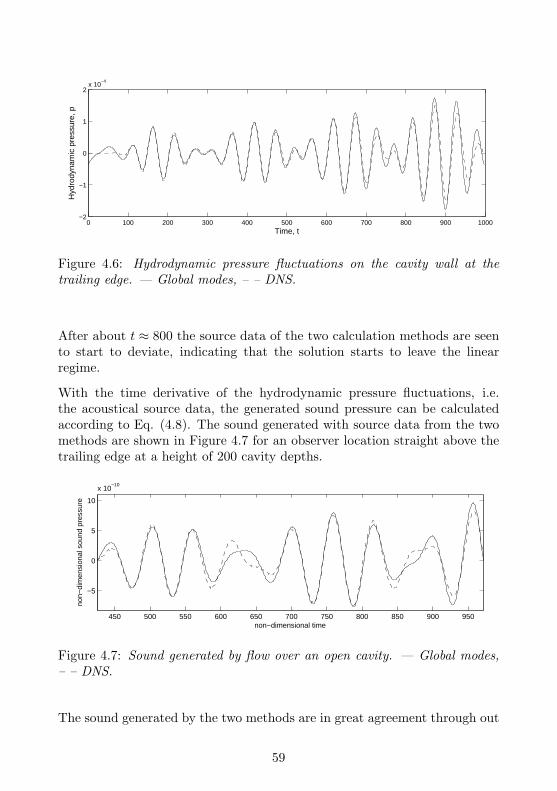
0 100 200 300 400 500 600 700 800 900 1000−2

−1

0

1

2x 10

−4

Time, t

Hyd

rody

nam

ic p

ress

ure,

p

Figure 4.6: Hydrodynamic pressure fluctuations on the cavity wall at thetrailing edge. — Global modes, – – DNS.

After about t ≈ 800 the source data of the two calculation methods are seento start to deviate, indicating that the solution starts to leave the linearregime.

With the time derivative of the hydrodynamic pressure fluctuations, i.e.the acoustical source data, the generated sound pressure can be calculatedaccording to Eq. (4.8). The sound generated with source data from the twomethods are shown in Figure 4.7 for an observer location straight above thetrailing edge at a height of 200 cavity depths.

450 500 550 600 650 700 750 800 850 900 950

−5

0

5

10

x 10−10

non−dimensional time

non−

dim

ensi

onal

sou

nd p

ress

ure

Figure 4.7: Sound generated by flow over an open cavity. — Global modes,– – DNS.

The sound generated by the two methods are in great agreement through out

59

the time sequence solved for, except in the nodes of the beatings, at t ≈ 630and t ≈ 880, where the sound is most sensitive of small errors in the sourcedata.

This example shows how the technique of global modes can be applied withgood accuracy at a low computational cost. In particular, the method issuitable to study the flow field structures related to acoustics, since a globalmode analysis reveal information on the presence of any unstable modeswhich can give rise to self-sustained oscillations and whistling. In particular,the method may be applied to predict whistling, or be used in combinationwith flow control to control flow generated noise levels.

60

Chapter 5

Conclusions andfuture work

Two simulation methodologies based on frequency domain formulations of thelinearized Navier-Stokes equations have been developed and evaluated withapplications related to the prediction of scattering of sound in flow ducts andwhistling.

The first method solves the propagation of sound waves directly by solvingthe compressible governing equations for the perturbations about a meanflow state. Both acoustic and vorticial perturbations are included and thusenables studies of vortex-sound interaction in cases of acoustic dissipation oramplifications due to vortex shedding. The method was applied to test casesof in-duct thin and thick orifice plates as well as area expansions.

To improve the method, implementations of cylindrical as well as fullthree dimensional geometries are needed. An implementation of the energyequation is needed in cases when the isentropic relation between density andpressure does not hold. Further validation on more complex geometries areneeded, as for example geometries with curved boundaries.

In the second method, an incompressible formulation of the linearized Navier-Stokes equations was solved as an eigenvalue problem to identify soundgenerating flow structures, and unstable flow structures related to whistling.The radiated sound was extracted through the use of Curle’s analogy, andthe method was applied to a test case of a shallow cavity. In future work,

61

the formulation may be extended to solve for the compressible equation, orthe global mode solver and the propagation methodology may be mergedsuch that the sound sources from the eigenmodes are incorporated in thefirst method to calculate the sound radiation from the individual modes.

62

Chapter 6

Summary of papers

Paper I

A frequency domain linearized Navier-Stokes equationsapproach to acoustic propagation in flow ducts with sharpedges.

A. Kierkegaard, S. Boij, G. Efraimsson

A methodology of a frequency domain linearized Navier-Stokes equationssolver was developed. Isentropic relations between perturbed pressure anddensity was assumed for simplification. The methodology was applied andevaluated on a 2D geometry of an aspect ratio η = 0.277 in-duct orifice platewith a M = 0.067 mean flow. No-slip boundary conditions were applied onthe orifice walls, but slip boundary conditions on the duct walls. Calculationswere carried out in a frequency range of 50-3000 Hz and the 2-port scatteringmatrix was calculated for all its four components. The simulations werecompared to measurements on a circular duct of same orifice diameter ratio bya normalized Helmholtz number technique, and good agreement was found.

63

Division of work between authors

Kierkegaard developed and implemented the methodology, performed thesimulations and wrote the paper under supervision of Efraimsson and Boij.

Paper II

Simulations of the Scattering of Sound Waves at a SuddenArea Expansion

A. Kierkegaard, S. Boij and G. Efraimsson

The scattering of acoustic plane waves at a sudden area expansion in a flowduct was simulated using the linearized Navier-Stokes methodology developedin Paper I. Transmission and reflection as well as end correction at the areaexpansion was simulated, and the influence of the downstream mean flowprofile on the acoustic scattering properties was investigated. A comparisonof results from numerical simulations, analytical theory and experimentswas presented. A study with realistic mean flow profiles for different Machnumbers, and two additional flow profiles, representing a non-expanding jetwith infinitely thin shear layer, and an immediate expansion, shows thata realistic jet is needed to accurately capture the acoustic-hydrodynamicinteraction. The prediction of the end correction for the constructed meanflow profiles deviates significantly from that for the realistic profile in aStrouhal number regime representing strong coupling between acoustic andhydrodynamic waves. It is concluded that the constructed flow profiles lackthe ability to predict the loss of energy to hydrodynamic waves, and that thiseffect increases with increasing Mach number.


Kierkegaard carried out the simulations. Boij derived the analytical solutions.The paper was jointly written by the authors.

64

Paper III

Simulations of whistling and the whistling potentiality ofan in-duct orifice with linear aeroacoustics

A. Kierkegaard, G. Efraimsson, S. Allam and M. Abom

The possibility to predict the whistling potentiality of an in-duct elementbased on linear aeroacoustic simulations was demonstrated, such that thegeometry can be modified to avoid whistling. The whistling potentialitywas investigated by an acoustic energy balance for the in-duct element andgood agreement with experimental data was shown. This indicates thatalthough whistling is a non-linear phenomena caused by an acoustic-flowinstability feed-back loop, the linearized Navier-Stokes equations can be usedto predict whistling potentiality. A Nyquist stability criterion was appliedto the simulation data to predict whistling, and results were compared toexperimental results with good agreement.


Kierkegaard carried out the simulations and Allam the experiments. Thepaper was jointly written by the authors.

Paper IV

Flow field eigenmode decompositions in aeroacoustics

A. Kierkegaard, E. Akervik, G. Efraimsson, D. S. Henningson

A flow field eigenvalue decomposition technique, so-called global modes, forlinear flows, was applied as source data to a far-field approximation of Curle’sequation. The main objective of the work was to evaluate the relevance ofthe global modes technique for aeroacoustic applications. As an exampleof an application, the sound generated from a 0.1 Mach number flow overan open cavity was calculated and compared to the sound generated froma DNS of an equivalent flow case. Small relative differences in input source

65

data between the methods were found to be amplified in the evaluation of theacoustic analogy integral. The over-all error levels in the calculated soundwas however well within an acceptable range. The main strength of theglobal modes technique was found in its possibility to isolate separate sound-generating mechanisms for detailed studies of sound generation processes.


Kierkegaard developed the Curle’s equation formulation for the global modesand carried out the acoustical calculations. Akervik calculated the globalmodes and the DNS. The paper was jointly written by the authors.

66

Bibliography

[1] B. Berglund, T. Lindvall, and D. H. Schwela. Guidlines for communitynoise. World Health Organization (WHO) report, 1999.

[2] H. G. Leventhall. Low frequency noise and annoyance. Noise & Health,6(23):59–72, 2004.

[3] M. J. Lighthill. On sound generated aerodynamically. I. General theory.Proc. Roy. Soc. Series A, 211(1107):564–587, 1952.

[4] T. Colonius, S. K. Lele, and P. Moin. Sound generation in a mixinglayer. J. Fluid Mech., 330:375–409, 1997.

[5] T. Colonius. and S. K. Lele. Computational aeroacoustics: progresson nonlinear problems. Progress in Aerospace Sciences, 40(6):345–416,2004.

[6] C. Bailly, C. Bogey, and X. Gloerfelt. Some useful hybrid approachesfor predicting aerodynamic noise. C. R. Mecanique, 333:666–675, 2005.

[7] M. Wang, J. B. Freund, and S. K. Lele. Computational prediction offlow-generated sound. Annu. Rev. Fluid Mech., Vol. 38:483–512, 2006.

[8] D. J. Bodony and S. K. Lele. Current status of jet noise predictionsusing large-eddy simulation. AIAA J., 46(2):364–380, 2008.

[9] C. Bailly, C. Bogey, and O. Marsden. Progress in direct noisecomputation. International Journal of Aeroacoustics, 9(1&2):123–143,2010.

[10] C. W. Rowley, T. Colonius, and A. J. Basu. On self-sustainedoscillations in two-dimensional compressible flow over rectangularcavities. J. Fluid Mech., 455:315–346, 2002.

67

[11] S. M. Grace. An overview of computational aeroacoustic techniquesapplied to cavity noise prediction. AIAA Paper 2001-0510, 39th AIAAAerospace Sciences Meeting and Exhibit, Reno, USA, 2001.

[12] J. Hardin and D. S. Pope. An acoustic/viscous splitting techniquefor computational aeroacoustics. Theoret. Comput. Fluid Dynamics,6:323–340, 1994.

[13] J. Hardin and D. S. Pope. Sound generation by flow over a two-dimensional cavity. AIAA J., 33(3):407–412, 1995.

[14] W. De Roeck, G. Rubio, M. Baelmans, and W. Desmet. Towardaccurate hybrid prediction techniques for cavity flow noise applications.Int. J. Numer. Meth. Fluids, 61:1363–1387, 2009.

[15] Y. Ozyoruk. Numerical prediction of aft radiation of turbofan tonesthrough exhaust jets. J. Sound Vib., 325(1-2):122–144, 2009.

[16] P. P. Rao and P. J. Morris. Use of finite element methods in frequencydomain aeroacoustics. AIAA J., 44(7):1643–1652, 2006.

[17] D. Casalino and M. Genito. Solution of linearized Lilley’s equation inthe frequency domain for turbofan aft noise prediction. AIAA Paper2007-3705, 13th AIAA/CEAS Aeroacoustics conference, Rome, Italy,2007.

[18] P. O. A. L. Davies. Piston enigine intake an exhaust system design. J.Sound Vib., 190(4):677–712, 1996.

[19] M. Abom. Measurement of the scattering-matrix of acoustical two-ports. Mechanical Systems and Signal Processing, 5(2):89–104, 1991.

[20] P. A. O. L. Davies. Practical flow duct acoustics. J. Sound Vib.,124(1):91–115, 1988.

[21] M. Knutsson and H. Boden. IC-engine acoustic source data from non-linear simulations. SAE Technical Paper 2007-01-2209, 2007.

[22] H. Boden and M. Abom. Modeling of fluid machines as sources of soundin duct and pipe systems. Acta Acustica, 3:549–560, 1995.

[23] K. S. Peat. Evaluation of four-pole parameters for ducts with flow bythe finite element method. J. Sound Vib., 84(3):389–395, 1982.

68

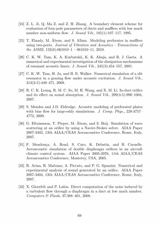
[24] Z. L. Ji, Q. Ma Z, and Z. H. Zhang. A boundary element scheme forevaluation of four-pole parameters of ducts and mufflers with low machnumber non-uniform flow. J. Sound Vib., 185(1):107–117, 1995.

[25] T. Elnady, M. Abom, and S. Allam. Modeling perforates in mufflersusing two-ports. Journal of Vibration and Acoustics - Transactions ofthe ASME, 132(6):061010–1 – 061010–11, 2010.

[26] C. K. W. Tam, K. A. Kurbatskii, K. K. Ahuja, and R. J. Gaeta. Anumerical and experimental investigation of the dissipation mechanismsof resonant acoustic liners. J. Sound Vib., 245(3):454–557, 2001.

[27] C. K .W. Tam, H. Ju, and B. E. Walker. Numerical simulation of a slitresonator in a grazing flow under acoustic excitation. J. Sound Vib.,313(3-5):449–471, 2008.

[28] R. C. K. Leung, R. M. C. So, M. H. Wang, and X. M. Li. In-duct orificeand its effect on sound absorption. J. Sound Vib., 299(4-5):990–1004,2007.

[29] S. Mendez and J.D. Eldredge. Acoustic modeling of perforated plateswith bias flow for large-eddy simulations. J. Comp. Phys., 228:4757–4772, 2009.

[30] G. Efraimsson, T. Pieper, M. Abom, and S. Boij. Simulation of wavescattering at an orifice by using a Navier-Stokes solver. AIAA Paper2007-3402, 13th AIAA/CEAS Aeroacoustics Conference, Rome, Italy,2007.

[31] F. Mendonca, A. Read, S. Caro, K. Debatin, and B. Caruelle.Aeroacoustic simulation of double diaphragm orifices in an aircraftclimate control system. AIAA Paper 2005-2976, 11th AIAA/CEASAeroacoustics Conference, Monterey, USA, 2005.

[32] R. Arina, R. Malvano, A. Piccato, and P. G. Spazzini. Numerical andexperimental analysis of sound generated by an orifice. AIAA Paper2007-3404, 13th AIAA/CEAS Aeroacoustics Conference, Rome, Italy,2007.

[33] X. Gloerfelt and P. Lafon. Direct computation of the noise induced bya turbulent flow through a diaphragm in a duct at low mach number.Computers & Fluids, 37:388–401, 2008.

69

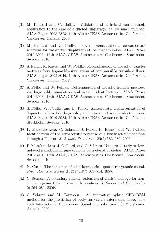
[34] M. Piellard and C. Bailly. Validation of a hybrid caa method.application to the case of a ducted diaphragm at low mach number.AIAA Paper 2008-2873, 14th AIAA/CEAS Aeroacoustics Conference,Vancouver, Canada, 2008.

[35] M. Piellard and C. Bailly. Several computational aeroacousticssolutions for the ducted diaphragm at low mach number. AIAA Paper2010-3996, 16th AIAA/CEAS Aeroacoustics Conference, Stockholm,Sweden, 2010.

[36] S. Foller, R. Kaess, and W. Polifke. Reconstruction of acoustic transfermatrices from large-eddy-simulations of compressible turbulent flows.AIAA Paper 2008-3046, 14th AIAA/CEAS Aeroacoustics Conference,Vancouver, Canada, 2008.

[37] S. Foller and W. Polifke. Determination of acoustic transfer matricesvia large eddy simulation and system identification. AIAA Paper2010-3998, 16th AIAA/CEAS Aeroacoustics Conference, Stockholm,Sweden, 2010.

[38] S. Foller, W. Polifke, and D. Tonon. Aeroacoustic characterization ofT-junctions based on large eddy simulation and system identification.AIAA Paper 2010-3985, 16th AIAA/CEAS Aeroacoustics Conference,Stockholm, Sweden, 2010.

[39] P. Martınez-Lera, C. Schram, S. Foller, R. Kaess, and W. Polifke.Identification of the aeroacoustic response of a low mach number flowthrough a T-joint. J. Acoust. Soc. Am., 126(2):582–586, 2009.

[40] P. Martınez-Lera, J. Golliard, and C. Schram. Numerical study of flow-induced pulsations in pipe systems with closed branches. AIAA Paper2010-3931, 16th AIAA/CEAS Aeroacoustics Conference, Stockholm,Sweden, 2010.

[41] N. Curle. The influence of solid boundaries upon aerodynamic sound.Proc. Roy. Soc. Series A, 231(1187):505–514, 1955.

[42] C. Schram. A boundary element extension of Curle’s analogy for non-compact geometries at low-mach numbers. J. Sound and Vib., 322(1-2):264–281, 2009.

[43] C. Schram and M. Tournour. An innovative hybrid CFD/BEMmethod for the prediction of body-turbulence interaction noise. The13th International Congress on Sound and Vibration (ISCV), Vienna,Austria, 2006.

70

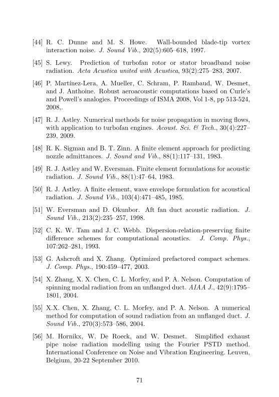
[44] R. C. Dunne and M. S. Howe. Wall-bounded blade-tip vortexinteraction noise. J. Sound Vib., 202(5):605–618, 1997.

[45] S. Lewy. Prediction of turbofan rotor or stator broadband noiseradiation. Acta Acustica united with Acustica, 93(2):275–283, 2007.

[46] P. Martınez-Lera, A. Mueller, C. Schram, P. Rambaud, W. Desmet,and J. Anthoine. Robust aeroacoustic computations based on Curle’sand Powell’s analogies. Proceedings of ISMA 2008, Vol 1-8, pp 513-524,2008,.

[47] R. J. Astley. Numerical methods for noise propagation in moving flows,with application to turbofan engines. Acoust. Sci. & Tech., 30(4):227–239, 2009.

[48] R. K. Sigman and B. T. Zinn. A finite element approach for predictingnozzle admittances. J. Sound and Vib., 88(1):117–131, 1983.

[49] R. J. Astley and W. Eversman. Finite element formulations for acousticradiation. J. Sound Vib., 88(1):47–64, 1983.

[50] R. J. Astley. A finite element, wave envelope formulation for acousticalradiation. J. Sound Vib., 103(4):471–485, 1985.

[51] W. Eversman and D. Okunbor. Aft fan duct acoustic radiation. J.Sound Vib., 213(2):235–257, 1998.

[52] C. K. W. Tam and J. C. Webb. Dispersion-relation-preserving finitedifference schemes for computational acoustics. J. Comp. Phys.,107:262–281, 1993.

[53] G. Ashcroft and X. Zhang. Optimized prefactored compact schemes.J. Comp. Phys., 190:459–477, 2003.

[54] X. Zhang, X. X. Chen, C. L. Morfey, and P. A. Nelson. Computation ofspinning modal radiation from an unflanged duct. AIAA J., 42(9):1795–1801, 2004.

[55] X.X. Chen, X. Zhang, C. L. Morfey, and P. A. Nelson. A numericalmethod for computation of sound radiation from an unflanged duct. J.Sound Vib., 270(3):573–586, 2004.

[56] M. Hornikx, W. De Roeck, and W. Desmet. Simplified exhaustpipe noise radiation modelling using the Fourier PSTD method.International Conference on Noise and Vibration Engineering. Leuven,Belgium, 20-22 September 2010.

71

[57] N. Schowald, L. Panek, C. Richter, and F. Thiele. Mode propagationin bifurcated bypass ducts: Application oriented simulation approach.AIAA Paper 2010-3895, 16th AIAA/CEAS Aeroacoustics Conference,Stockholm, Sweden, 2010.

[58] X. X. Chen, X. Huang, and . Zhang. Sound radiation from a bypassduct with bifurcations. AIAA J., 47(2):429–436, 2009.

[59] X. Huang, X. Chen, Z. Ma, and X. Zhang. Efficient computation ofspinning modal radiation through an engine bypass duct. AIAA J.,46(6):1413–1423, 2008.

[60] R. Ewert and W. Schroder. Acoustic perturbation equations based onflow decomposition via source filtering. J. Comp. Phys., 188:365–398,2003.

[61] F. Bassi and S. Rebay. High order accurate discontinuous finite elementsolution of the 2D Euler equations. J. Comp. Phys., 138:251–285, 1997.

[62] R. Leneveu, B. Schiltz, S. Laldjee, and S. Caro. Performance of aDGM scheme for LEE and applications to aircraft engine exhaust noise.AIAA Paper 2008-2884, 14th AIAA/CEAS Aeroacoustics Conference,Vancouver, Canada, 2008.

[63] Y. Ozyoruk, E. Alpman, V. Ahuja, and L. N. Long. Frequency-domainprediction of turbofan noise radiation. J. Sound Vib., 270(4-5):933–950,2004.

[64] Y. Ozyoruk, E. Dizemeny, S. Kayay, and A. Akturkz. Afrequency domain linearized Euler solver for turbomachinery noisepropagation and radiation. AIAA Paper 2007-3521, 13th AIAA/CEASAeroacoustics conference, Rome, Italy, 2007.

[65] Y. Ozyoruk and B. J. Tester. Assessment of a frequency-domainlinearised Euler solver for turbofan aft radiation predictions andcomparison with measurements. Procedia Engineering, 6:153–162, 2010.

[66] G. Gabard. Wave-based discontinuous Galerkin methods for thelinearized Euler equations in the frequency domain. AIAA Paper 2007-3476, 13th AIAA/CEAS Aeroacoustics Conference, Rome, Italy, 2007.

[67] G. Gabard. Discontinuous Galerkin methods with plane waves for time-harmonic problems. J. Comp. Phys., 225(2):1961–1984, 2007.

72

[68] A. Iob, R. Arina, and C. Schipani. Frequency-domain linearized Eulermodel for turbomachinery noise radiation through engine exhaust.AIAA J., 48(4):848–858, 2010.

[69] M. O. Burak, M. Billson, L. E. Eriksson, and S. Baralon. Validation ofa time- and frequency-domain grazing flow acoustic liner model. AIAAJ., 47(8):1841–1848, 2009.

[70] D. Casalino, M. Roger, and M. C. Jacob. Prediction ofsound propagation in ducted potential flows using Green’s functiondiscretization. AIAA J., 42(4):736–744, 2004.

[71] D. Casalino and M. Genito. Turbofan aft noise predictions based onLilley’s wave model. AIAA J., 46(1):84–93, 2008.

[72] D. Casalino and M. Genito. Achievements in the numerical modelingof fan noise radiation from aero-engines. Aerospace Science andTechnology, 12:105–113, 2008.

[73] M. Genito and D. Casalino. Numerical modeling of sound diffractionat a half-plane trailing edge. AIAA J., 46(4):958–966, 2008.

[74] D. Casalino. Benchmarking of different wave models for soundpropagation in non-uniform flows. Procedia Engineering, 6:163–172,2010.

[75] F. Treyssede, G. Gabard, and M. Ben Tahar. A mixed finite elementmethod for acoustic wave propagation in moving fluids based on anEulerian-Lagrangian description. J. Acoust. Soc. Am., 113(2):705–716,2003.

[76] D. Casalino and D. Bodony. Green’s function discretization ofPridmore-Brown wave operator. Center for Turbulence Research,Proceedings of the Summer Program, 547-558, 2006.

[77] P. G. Drazin and W. H. Reid. Hydrodynamic stability. Cambridge Univ.Press, Cambridge, 1981.

[78] P.J. Schmidt and D.S. Henningson. Stability and Transition in ShearFlows. Springer, Berlin, 2001.

[79] A. Michalke. On spatially growing disturbances in an inviscid shearlayer. J. Fluid Mech., 23(3):521–544, 1965.

73

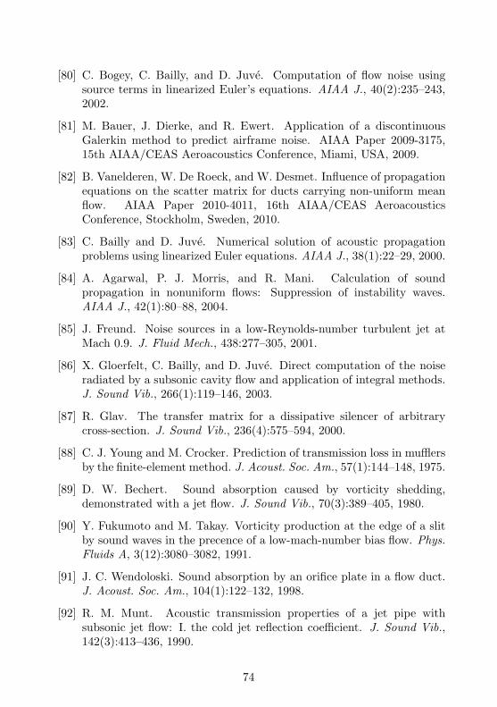
[80] C. Bogey, C. Bailly, and D. Juve. Computation of flow noise usingsource terms in linearized Euler’s equations. AIAA J., 40(2):235–243,2002.

[81] M. Bauer, J. Dierke, and R. Ewert. Application of a discontinuousGalerkin method to predict airframe noise. AIAA Paper 2009-3175,15th AIAA/CEAS Aeroacoustics Conference, Miami, USA, 2009.

[82] B. Vanelderen, W. De Roeck, and W. Desmet. Influence of propagationequations on the scatter matrix for ducts carrying non-uniform meanflow. AIAA Paper 2010-4011, 16th AIAA/CEAS AeroacousticsConference, Stockholm, Sweden, 2010.

[83] C. Bailly and D. Juve. Numerical solution of acoustic propagationproblems using linearized Euler equations. AIAA J., 38(1):22–29, 2000.

[84] A. Agarwal, P. J. Morris, and R. Mani. Calculation of soundpropagation in nonuniform flows: Suppression of instability waves.AIAA J., 42(1):80–88, 2004.

[85] J. Freund. Noise sources in a low-Reynolds-number turbulent jet atMach 0.9. J. Fluid Mech., 438:277–305, 2001.

[86] X. Gloerfelt, C. Bailly, and D. Juve. Direct computation of the noiseradiated by a subsonic cavity flow and application of integral methods.J. Sound Vib., 266(1):119–146, 2003.

[87] R. Glav. The transfer matrix for a dissipative silencer of arbitrarycross-section. J. Sound Vib., 236(4):575–594, 2000.

[88] C. J. Young and M. Crocker. Prediction of transmission loss in mufflersby the finite-element method. J. Acoust. Soc. Am., 57(1):144–148, 1975.

[89] D. W. Bechert. Sound absorption caused by vorticity shedding,demonstrated with a jet flow. J. Sound Vib., 70(3):389–405, 1980.

[90] Y. Fukumoto and M. Takay. Vorticity production at the edge of a slitby sound waves in the precence of a low-mach-number bias flow. Phys.Fluids A, 3(12):3080–3082, 1991.

[91] J. C. Wendoloski. Sound absorption by an orifice plate in a flow duct.J. Acoust. Soc. Am., 104(1):122–132, 1998.

[92] R. M. Munt. Acoustic transmission properties of a jet pipe withsubsonic jet flow: I. the cold jet reflection coefficient. J. Sound Vib.,142(3):413–436, 1990.

74

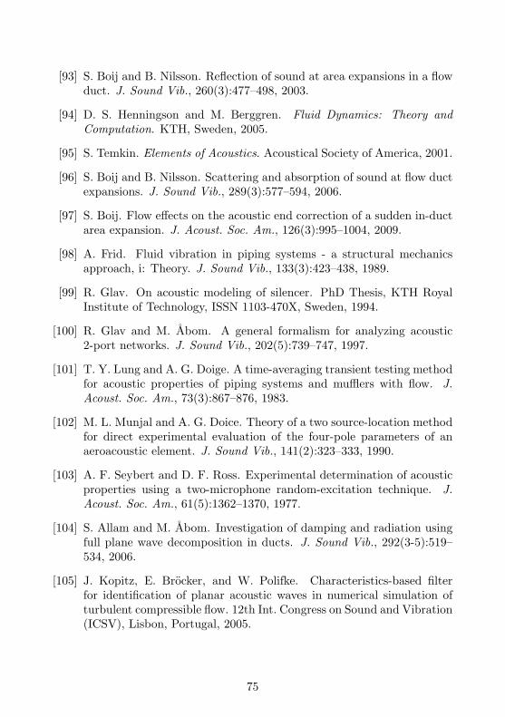
[93] S. Boij and B. Nilsson. Reflection of sound at area expansions in a flowduct. J. Sound Vib., 260(3):477–498, 2003.

[94] D. S. Henningson and M. Berggren. Fluid Dynamics: Theory andComputation. KTH, Sweden, 2005.

[95] S. Temkin. Elements of Acoustics. Acoustical Society of America, 2001.

[96] S. Boij and B. Nilsson. Scattering and absorption of sound at flow ductexpansions. J. Sound Vib., 289(3):577–594, 2006.

[97] S. Boij. Flow effects on the acoustic end correction of a sudden in-ductarea expansion. J. Acoust. Soc. Am., 126(3):995–1004, 2009.

[98] A. Frid. Fluid vibration in piping systems - a structural mechanicsapproach, i: Theory. J. Sound Vib., 133(3):423–438, 1989.

[99] R. Glav. On acoustic modeling of silencer. PhD Thesis, KTH RoyalInstitute of Technology, ISSN 1103-470X, Sweden, 1994.

[100] R. Glav and M. Abom. A general formalism for analyzing acoustic2-port networks. J. Sound Vib., 202(5):739–747, 1997.

[101] T. Y. Lung and A. G. Doige. A time-averaging transient testing methodfor acoustic properties of piping systems and mufflers with flow. J.Acoust. Soc. Am., 73(3):867–876, 1983.

[102] M. L. Munjal and A. G. Doice. Theory of a two source-location methodfor direct experimental evaluation of the four-pole parameters of anaeroacoustic element. J. Sound Vib., 141(2):323–333, 1990.

[103] A. F. Seybert and D. F. Ross. Experimental determination of acousticproperties using a two-microphone random-excitation technique. J.Acoust. Soc. Am., 61(5):1362–1370, 1977.

[104] S. Allam and M. Abom. Investigation of damping and radiation usingfull plane wave decomposition in ducts. J. Sound Vib., 292(3-5):519–534, 2006.

[105] J. Kopitz, E. Brocker, and W. Polifke. Characteristics-based filterfor identification of planar acoustic waves in numerical simulation ofturbulent compressible flow. 12th Int. Congress on Sound and Vibration(ICSV), Lisbon, Portugal, 2005.

75

[106] E. Alenius. CFD of duct acoustics for turbocharger applications, Lic.Tech. thesis. KTH Royal Institute of Technology, Stockholm, Sweden,2010.

[107] M. Abom, S. Allam, and S. Boij. Aero-acoustics of flow ductsingularities at low mach numbers. AIAA Paper 2006-2687, 12thAIAA/CEAS Aeroacoustics Conference, Cambridge, USA, 2006.

[108] D. Ronneberger. Theoretische und experimentelle untersuchungder schallausbreitung durch querschnitts-sprunge und lochplatten instromungskanalen. Technical report, DFG-Abschlussbericht, DrittesPhysikalisches Institut der Universitat Gottingen, 1987.

[109] P. Testud, Y. Auregan, P. Moussou, and A. Hirschberg. The whistlingpotentiality of an orifice in a confined flow using an energetic criterion.J. Sound Vib., 325(4-5):769–780, 2009.

[110] P. Durrieu, G. Hofmans, G. Ajello, R. Boot, Y. Auregan, A. Hirschberg,, and M. C. A. M. Peters. Quasisteady aero-acoustic response of orifices.J. Acoust. Soc. Am., 110(4):1859–1872, 2001.

[111] A. Kierkegaard and G. Efraimsson. Generation and propagation ofsound waves in low mach number flows. AIAA Paper 2007-3485, 13thAIAA/CEAS Aeroacoustics conference, Rome, Italy, 2007.

[112] M. H. Carpenter, J. Nordstrom, and D. Gottlieb. A stable andconservative interface treatment of arbitrary spatial accuracy. J. Comp.Phys., 148(2):341–365, 1999.

[113] K. Mattsson, M. Svard, and J. Nordstrom. Stable and accurate artificialdissipation. Journal of Scientific Computing, 21(1):57–79, 2004.

[114] K. Mattsson and J. Nordstrom. Summation by parts operators forfinite difference approximations of second derivatives. J. Comp. Phys.,199(2):503–540, 2004.

[115] J. Nordstrom and M. H. Carpenter. Boundary and interface conditionsfor high order finite difference methods applied to the Euler and Navier-Stokes equations. J. Comp. Phys., 148(2):621–645, 1999.

[116] J. Nordstrom and M. H. Carpenter. High order finite difference meth-ods, multi-dimensional linear problems and curvilinear coordinates. J.Comp. Phys., 173(1):149–174, 2001.

76

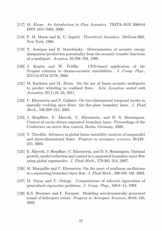
[117] M. Abom. An Introduction to Flow Acoustics. TRITA-AVE 2006:04ISSN 1651-7660, 2006.

[118] P. M. Morse and K. U. Ingard. Theoretical Acoustics. McGraw-Hill,New York, 1968.

[119] Y. Auregan and R. Starobinsky. Determination of acoustic energydissipation/production potentiality from the acoustic transfer functionsof a multiport. Acustica, 85:788–792, 1999.

[120] J. Kopitz and W. Polifke. CFD-based application of theNyquist criterion to thermo-acoustic instabilities. J. Comp. Phys.,227(14):6754–6778, 2008.

[121] M. Karlsson and M. Abom. On the use of linear acoustic multiportsto predict whistling in confined flows. Acta Acoustica united withAcoustica, 97(1):24–33, 2011.

[122] U. Ehrenstein and F. Gallaire. On two-dimensional temporal modes inspatially evolving open flows: the flat-plate boundary layer. J. FluidMech., 536:209–218, 2005.

[123] J. Hœpffner, E. Akervik, U. Ehrenstein, and D. S. Henningson.Control of cavity-driven separated boundary layer. Proceedings of theConference on active flow control, Berlin, Germany, 2006.

[124] V. Theofilis. Advances in global linear instability analysis of nonparalleland three-dimensional flows. Progress in aerospace sciences, 39:249–315, 2003.

[125] E. Akervik, J. Hœpffner, U. Ehrenstein, and D. S. Henningson. Optimalgrowth, model reduction and control in a separated boundary-layer flowusing global eigenmodes. J. Fluid Mech., 579:305–314, 2007.

[126] M. Marquillie and U. Ehrenstein. On the onset of nonlinear oscillationsin a separating boundary-layer flow. J. Fluid Mech., 490:169–188, 2003.

[127] M. Nayar and U. Ortega. Computations of selected eigenvalues ofgeneralized eigenvalue problems. J. Comp. Phys., 108:8–14, 1993.

[128] K.S. Brentner and F. Farassat. Modeling aerodynamically generatedsound of helicopter rotors. Progress in Aerospace Sciences, 39:83–120,2003.

77

[129] F. Farassat. Theory of noise generation from moving bodies withapplication to helicopter rotors. NASA TR-451, 1975.

[130] K.S. Brentner. Numerical algorithms for acoustic integrals withexamples for rotor noise prediction. AIAA J., 35(4):625–630, 1997.

[131] D. Casalino. An advanced time approach for acoustic analogypredictions. J. Sound Vib., 261(4):583–612, 2003.

[132] S. Sarkar and M.Y. Hussaini. Computation of the acoustic radiationfrom bounded homogeneous flows. Computational Aeroacoustics,Springer, 1993.

[133] A. Kierkegaard and G. Efraimsson. A study of interpolation accuracy inacoustic analogy integrals. AIAA Paper 2010-3997, 16th AIAA/CEASAeroacoustic conference, Stockholm, Sweden, 2010.

78

frequency domain linearized navier-stokes...

Documents