frequency analysis: the fourier series · responds to the fourier transform of the convolution...

CHAPTER 4

Frequency Analysis: The FourierSer ies

A Mathematician is a device forturning coffee into theorems.

Paul Erdos (1913–1996)mathematician

4.1 INTRODUCTIONIn this chapter and the next we consider the frequency analysis of continuous-time signals andsystems—the Fourier series for periodic signals in this chapter, and the Fourier transform for bothperiodic and aperiodic signals as well as for systems in Chapter 5. In these chapters we consider:

n Spectral representation—The frequency representation of periodic and aperiodic signals indicateshow their power or energy is allocated to different frequencies. Such a distribution over frequencyis called the spectrum of the signal. For a periodic signal the spectrum is discrete, as its poweris concentrated at frequencies multiples of a so-called fundamental frequency, directly related tothe period of the signal. On the other hand, the spectrum of an aperiodic signal is a contin-uous function of frequency. The concept of spectrum is similar to the one used in optics forlight, or in material science for metals, each indicating the distribution of power or energy overfrequency. The Fourier representation is also useful in finding the frequency response of lineartime-invariant systems, which is related to the transfer function obtained with the Laplace trans-form. The frequency response of a system indicates how an LTI system responds to sinusoids ofdifferent frequencies. Such a response characterizes the system and permits easy computation ofits steady-state response, and will be equally important in the synthesis of systems.

n Eigenfunctions and Fourier analysis—It is important to understand the driving force behind therepresentation of signals in terms of basic signals when applied to LTI systems. For instance, theconvolution integral that gives the output of an LTI system resulted from the representation of itsinput signal in terms of shifted impulses. Along with this result came the concept of the impulseresponse of an LTI system. Likewise, the Laplace transform can be seen as the representation ofsignals in terms of general eigenfunctions. In this chapter and the next we will see that complex

Systems and Signals Using MATLAB. DOI: 10.1016/B978-0-12-374716-7.00007-7c© 2011, Elsevier Inc. All rights reserved. 237

238 CHAPTER 4: Frequency Analysis: The Fourier Series

exponentials or sinusoids are used in the Fourier representation of periodic as well as aperiodicsignals by taking advantage of the eigenfunction property of LTI systems. The results of the Fourierseries in this chapter will be extended to the Fourier transform in Chapter 5.

n Steady-state analysis—Fourier analysis is in the steady state, while Laplace analysis considers bothtransient and steady state. Thus, if one is interested in transients, as in control theory, Laplace isa meaningful transformation. On the other hand, if one is interested in the frequency analysis,or steady state, as in communications theory, the Fourier transform is the one to use. There willbe cases, however, where in control and communications both Laplace and Fourier analysis areconsidered.

n Application of Fourier analysis—The frequency representation of signals and systems is extremelyimportant in signal processing and in communications. It explains filtering, modulation of mes-sages in a communication system, the meaning of bandwidth, and how to design filters. Likewise,the frequency representation turns out to be essential in the sampling of analog signals—thebridge between analog and digital signal processing.

4.2 EIGENFUNCTIONS REVISITEDAs indicated in Chapter 3, the most important property of stable LTI systems is that when the inputis a complex exponential (or a combination of a cosine and a sine) of a certain frequency, the outputof the system is the input times a complex constant connected with how the system responds to thefrequency at the input. The complex exponential is called an eigenfunction of stable LTI systems.

If x(t) = ej0t , −∞ < t <∞, is the input to a causal and a stable system with impulse response h(t), theoutput in the steady state is given by

y(t) = ej0tH( j0) (4.1)

where

H( j0) =

∞∫0

h(τ )e−j0τ dτ (4.2)

is the frequency response of the system at 0. The signal x(t) = ej0t is said to be an eigenfunction of the LTIsystem as it appears at both input and output.

This can be seen by finding the output corresponding to x(t) = ej0t by means of the convolutionintegral,

y(t) =

∞∫0

h(τ )x(t − τ)dτ = ej0t

∞∫0

h(τ )e−j0τdτ

= ej0tH( j0)

4.2 Eigenfunctions Revisited 239

where we let H( j0) equal the integral in the second equation. The input signal appears in the outputmodified by the frequency response of the system H( j0) at the frequency 0 of the input. Noticethat the convolution integral limits indicate that the input started at −∞ and that we are consideringthe output at finite time t—this means that we are in steady state. The steady-state response of astable LTI system is attained by either considering that the initial time when the input is applied tothe system is −∞ and we reach a finite time t, or by starting at time 0 and going to∞.

The above result for one frequency can be easily extended to the case of several frequencies presentat the input. If the input signal x(t) is a linear combination of complex exponentials, with differentamplitudes, frequencies, and phases, or

x(t) =∑

k

Xkejkt

where Xk are complex values, since the output corresponding to Xkejkt is XkejktH( jk) bysuperposition the response to x(t) is

y(t) =∑

k

XkejktH( jk)

=

∑k

Xk|H( jk)|ej(kt+∠H( jk)) (4.3)

The above is valid for any signal that is a combination of exponentials of arbitrary frequencies. As wewill see in this chapter, when x(t) is periodic it can be represented by the Fourier series, which is acombination of complex exponentials harmonically related (i.e., the frequencies of the exponentialsare multiples of the fundamental frequency of the periodic signal). Thus, when a periodic signal isapplied to a causal and stable LTI system its output is computed as in Equation (4.3).

The significance of the eigenfunction property is also seen when the input signal is an integral(a sum, after all) of complex exponentials, with continuously varying frequency, as the integrand.That is, if

x(t) =1

2π

∞∫−∞

X()ejtd

then using superposition and the eigenfunction property of a stable LTI system, with frequencyresponse H( j), the output is

y(t) =1

2π

∞∫−∞

X()ejtH( j)d

=1

2π

∞∫−∞

X()|H( j)|e( jt+j∠H( j))d (4.4)


The above representation of x(t) corresponds to the Fourier representation of aperiodic signals, whichwill be covered in Chapter 5. Again here, the eigenfunction property of LTI systems provides an effi-cient way to compute the output. Furthermore, we also find that by letting Y() = X()H( j) theabove equation gives an expression to compute y(t) from Y(). The product Y() = X()H( j) cor-responds to the Fourier transform of the convolution integral y(t) = x(t) ∗ h(t), and is connected withthe convolution property of the Laplace transform. It is important to start noticing these connections,to understand the link between Laplace and Fourier analysis.

Remarks

n Notice the difference of notation for the frequency representation of signals and systems used above. If x(t)is a periodic signal its frequency representation is given by Xk, and if aperiodic by X(), while for asystem with impulse response h(t) its frequency response is given by H( j).

n When considering the eigenfunction property, the stability of the LTI system is necessary to ensure thatH( j) exists for all frequencies.

n The eigenfunction property applied to a linear circuit gives the same result as the one obtained from phasorsin the sinusoidal steady state. That is, if

x(t) = A cos(0t + θ) =Aejθ

2ej0t+

Ae−jθ

2e−j0t (4.5)

is the input of a circuit represented by the transfer function

H(s) =Y(s)X(s)=L[y(t)]L[x(t)]

then the corresponding steady-state output is given by

yss(t) =Aejθ

2ej0tH( j0)+

Ae−jθ

2e−j0tH(−j0)

= A|H( j0)| cos(0t + θ + ∠H( j0)) (4.6)

where, very importantly, the frequency of the output coincides with that of the input, and the amplitudeand phase of the input are changed by the magnitude and phase of the frequency response of the systemfor the frequency 0. The frequency response is H( j0) = H(s)|s=j0 , and as we will see its magnitudeis an even function of frequency, or |H( j)| = |H(−j)|, and its phase is an odd function of frequency,or ∠H( j0) = −∠H(−j0). Using these two conditions we obtain Equation (4.6).The phasor corresponding to the input

x(t) = A cos(0t + θ)

is defined as a vector,

X = A∠θ

rotating in the polar plane at the frequency of 0. The phasor has a magnitude A and an angle θ withrespect to the positive real axis. The projection of the phasor onto the real axis, as it rotates at the given


frequency, with time generates a cosine of the indicated frequency, amplitude, and phase. The transferfunction is computed at s = j0 or

H(s)|s=j0 = H( j0) =YX

(ratio of the phasors corresponding to the output Y and the input X). The phasor for the outputis thus

Y = H( j0)X = |Y|ej∠Y

Such a phasor is then converted into the sinusoid (which equals Eq. 4.6):

yss(t) = Re[Yej0t] = |Y| cos(0t + ∠Y)

n A very important application of LTI systems is filtering, where one is interested in preserving desiredfrequency components of a signal and getting rid of less-desirable components. That an LTI system can beused for filtering is seen in Equations (4.3) and (4.4). In the case of a periodic signal, the magnitude|H( jk)| can be set ideally to one for those components we wish to keep and to zero for those we wishto get rid of. Likewise, for an aperiodic signal, the magnitude |H( j)| could be set ideally to one forthose components we wish to keep and zero for those components we wish to get rid of. Depending onthe filtering application, an LTI system with the appropriate characteristics can be designed, obtaining thedesired transfer function H(s).

For a stable LTI with transfer function H(s) if the input is

x(t) = Re[Aej(0t+θ)] = A cos(0t + θ)

the steady-state output is given by

y(t) = Re[AH( j0)ej(0t+θ)]

= A|H( j0)| cos(0t + θ +∠H( j0)) (4.7)

where

H( j0) = H(s)|s=j0

n Example 4.1Consider the RC circuit shown in Figure 4.1. Let the voltage source be vs(t) = 4 cos(t + π/4) volts.the resistor be R = 1, and the capacitor C = 1 F. Find the steady-state voltage across the capacitor.

Solution

This problem can be approached in two ways.

n Phasor approach. From the phasor circuit in Figure 4.1, by voltage division we have the follow-ing phasor ratio, where Vs is the phasor corresponding to the source vs(t) and Vc the phasor


FIGURE 4.1RC circuit and corresponding phasorcircuit.

vs (t)

1Ω

1F vc (t)

+

− +

−

1

−j

+

−Vc

+

−

Vs

corresponding to vc(t):

Vc

Vs=−j

1− j=−j(1+ j)

2=

√2

2∠−π/4

Since Vs = 4∠π/4, then

Vc = 2√

2∠0

so that in the steady state,

vc(t) = 2√

2 cos(t)

n Eigenfunction approach. Considering the output is the voltage across the capacitor and the inputis the voltage source, the transfer function is obtained using voltage division as

H(s) =Vc(s)Vs(s)

=1/s

1+ 1/s=

1s+ 1

so that the system frequency response at the input frequency 0 = 1 is

H( j1) =

√2

2∠−π/4

According to the eigenfunction property the steady-state response of the capacitor is

vc(t) = 4|H( j1)| cos(t + π/4+ ∠H( j1))

= 2√

2 cos(t)

which coincides with the solution found using phasors. n

n Example 4.2An ideal communication system provides as output the input signal with only a possible delay inthe transmission. Such an ideal system does not cause any distortion to the input signal beyond


the delay. Find the frequency response of the ideal communication system, and use it to determinethe steady-state response when the delay caused by the system is τ = 3 sec, and the input is x(t) =2 cos(4t − π/4).

Solution

The impulse response of the ideal system is h(t) = δ(t − τ)where τ is the delay of the transmission.In fact, the output according to the convolution integral gives

y(t) =

∞∫0

δ(ρ − τ)︸︷︷︸h(ρ)

x(t − ρ)dρ = x(t − τ)

as expected. Let us then find the frequency response of the ideal communication system. Accordingto the eigenvalue property, if the input is x(t) = ej0t, then the output is

y(t) = ej0tH( j0)

but also

y(t) = x(t − τ) = ej0(t−τ)

so that comparing these equations we have that

H( j0) = e−jτ0

For a generic frequency 0 ≤ <∞, we would get

H( j) = e−jτ

which is a complex function of , with a unity magnitude |H( j)| = 1, and a linear phase∠H( j) = −τ. This system is called an all-pass system, since it allows all frequency componentsof the input to go through with a phase change only.

Consider the case when τ = 3, and that we input into this system x(t) = 2 cos(4t − π/4), thenH( j) = 1e−j3, so that the output in the steady state is

y(t) = 2|H( j4)| cos(4t − π/4+ ∠H( j4))

= 2 cos(4(t − 3)− π/4)

= x(t − 3)

where we used H( j4) = 1e−j12 (i.e., |H( j4)| = 1 and ∠H( j4) = 12). n

n Example 4.3Although there are better methods to compute the frequency response of a system represented bya differential equation, the eigenfunction property can be easily used for that. Consider the RC


circuit shown in Figure 4.1 where the input is

vs(t) = 1+ cos(10,000t)

with components of low frequency, = 0, and of large frequency, = 10,000 rad/sec. The outputvc(t) is the voltage across the capacitor in steady state. We wish to find the frequency response ofthis circuit to verify that it is a low-pass filter (it allows low-frequency components to go through,but filters out high-frequency components).

Solution

Using Kirchhoff’s voltage law, this circuit is represented by a first-order differential equation,

vs(t) = vc(t)+dvc(t)

dt

Now, if the input is vs(t) = ejt, for a generic frequency , then the output is vc(t) = ejtH( j).Replacing these in the differential equation, we have

ejt= ejtH( j)+

dejtH( j)dt

= ejtH( j)+ jejtH( j)

so that

H( j) =1

1+ j

or the frequency response of the filter for any frequency . The magnitude of H( j) is

|H( j)| =1

√1+2

which is close to one for small values of the frequency, and tends to zero when the frequencyvalues are large—the characteristics of a low-pass filter.

For the input

vs(t) = 1+ cos(10,000t) = cos(0t)+ cos(10,000t)

(i.e., it has a zero frequency component and a 10,000-rad/sec frequency component) using Euler’sidentity, we have that

vs(t) = 1+ 0.5(ej10,000t

+ e−j10,000t)

and the steady-state output of the circuit is

vc(t) = 1H( j0)+ 0.5H( j10,000)ej10,000t+ 0.5H(−j10,000)e−j10,000t

≈ 1+1

10,000cos(10,000t − π/2) ≈ 1

4.3 Complex Exponential Fourier Series 245

since

H( j0) = 1

H( j10,000) ≈1

j 104 =−j

10,000

H(−j10,000) ≈1

−j 104 =j

10,000

Thus, this circuit acts like a low-pass filter by keeping the DC component (with the low frequency = 0) and essentially getting rid of the high-frequency ( = 10,000) component of the signal.

Notice that the frequency response can also be obtained by considering the phasor ratio for ageneric frequency , which by voltage division is

Vc

Vs=

1/j1+ 1/j

=1

1+ j

which for = 0 is 1 and for = 10,000 is approximately −j/10,000 (i.e., corresponding to H( j0)and H( j10,000) = H∗( j10,000)). n

Fourier and Laplace

French mathematician Jean-Baptiste-Joseph Fourier (1768–1830) was a contemporary of Laplace with whom he sharedmany scientific and political experiences [2, 7]. Like Laplace, Fourier was from very humble origins but he was not aspolitically astute. Laplace and Fourier were affected by the political turmoil of the French Revolution and both came in closecontact with Napoleon Bonaparte, French general and emperor. Named chair of the mathematics department of the EcoleNormale, Fourier led the most brilliant period of mathematics and science education in France. His main work was “TheMathematical Theory of Heat Conduction” where he proposed the harmonic analysis of periodic signals. In 1807 he receivedthe grand prize from the French Academy of Sciences for this work. This was despite the objections of Laplace, Lagrange,and Legendre, who were the referees and who indicated that the mathematical treatment lacked rigor. Following Galton’sadvice of “Never resent criticism, and never answer it,” Fourier disregarded these criticisms and made no change to his1822 treatise in heat conduction. Although Fourier was an enthusiast for the Revolution and followed Napoleon on someof his campaigns, in the Second Restoration he had to pawn his belongings to survive. Thanks to his friends, he becamesecretary of the French Academy, the final position he held.

4.3 COMPLEX EXPONENTIAL FOURIER SERIESThe Fourier series is a representation of a periodic signal x(t) in terms of complex exponentials orsinusoids of frequency multiples of the fundamental frequency of x(t). The advantage of using theFourier series to represent periodic signals is not only the spectral characterization obtained, but infinding the response for these signals when applied to LTI systems by means of the eigenfunctionproperty.

Mathematically, the Fourier series is an expansion of periodic signals in terms of normalized orthog-onal complex exponentials. The concept of orthogonality of functions is similar to the concept of


perpendicularity of vectors: Perpendicular vectors cannot be represented in terms of each other, asorthogonal functions provide mutually exclusive information. The perpendicularity of two vectorscan be established using the dot or scalar product of the vectors, and the orthogonality of functions isestablished by the inner product, or the integration of the product of the function and its conjugate.Consider a set of complex functions ψk(t) defined in an interval [a, b], and such that for any pair ofthese functions, let’s say ψ`(t) and ψm(t), ` 6= m, their inner product is

b∫a

ψ`(t)ψ∗m(t)dt =

0 ` 6= m1 ` = m

(4.8)

Such a set of functions is called orthonormal (i.e., orthogonal and normalized).

A finite-energy signal x(t) defined in [a, b] can be approximated by a series

x(t) =∑

k

akψk(t) (4.9)

according to some error criterion. For instance, we could minimize the energy of the error functionε(t) = x(t)− x(t) or

b∫a

|ε(t)|2dt =

b∫a

∣∣∣∣∣x(t)−∑k

akψk(t)

∣∣∣∣∣2

dt (4.10)

The expansion can be finite or infinite, and may not approximate the signal point by point.

Fourier proposed sinusoids as the functions ψk(t) to represent periodic signals, and solved thequadratic minimization posed in Equation (4.10) to obtain the coefficients of the representation.For most signals, the resulting Fourier series has an infinite number of terms and coincides with thesignal pointwise. We will start with a more general expansion that uses complex exponentials andfrom it obtain the sinusoidal form. In Chapter 5 we extend the Fourier series to represent aperiodicsignals—leading to the Fourier transform that is in turn connected with the Laplace transform.

Recall that a periodic signal x(t) is such that

n It is defined for −∞ < t <∞ (i.e., it has an infinite support).n For any integer k, x(t + kT0) = x(t), where T0 is the fundamental period of the signal or the

smallest positive real number that makes this possible.

The Fourier series representation of a periodic signal x(t), of period T0, is given by an infinite sum of weightedcomplex exponentials (cosines and sines) with frequencies multiples of the signal’s fundamental frequency0 = 2π/T0 rad/sec, or

x(t) =∞∑

k=−∞

Xkejk0t 0 =2πT0

(4.11)

4.3 Complex Exponential Fourier Series 247

where the Fourier coefficients Xk are found according to

Xk =1T0

t0+T0∫t0

x(t)e−jk0tdt (4.12)

for k = 0,±1,±2, . . . , and any t0. The form of Equation (4.12) indicates that the information needed for theFourier series can be obtained from any period of x(t).

Remarks

n The Fourier series uses the Fourier basis ejk0t, k integer to represent the periodic signal x(t) of periodT0. The Fourier basis functions are also periodic of period T0 (i.e., for an integer m,

ejk0(t+mT0) = ejk0tejkm2π= ejk0t

as ejkm2π= 1).

n The Fourier basis functions are orthonormal over a period—that is,

1T0

t0+T0∫t0

ejk0t[ej`0t]∗dt =

1 k = `

0 k 6= `(4.13)

That is, ejk0t and ej`0t are said to be orthogonal when for k 6= ` the above integral is zero, and theyare normal (or normalized) when for k = ` the above integral is unity. The functions ejk0t and ej`0t

are orthogonal since

1T0

t0+T0∫t0

ejk0t[ej`0t]∗ dt =1T0

t0+T0∫t0

ej(k−`)0tdt

=1T0

t0+T0∫t0

[cos((k− `)0t)+ j sin((k− `)0t)] dt

= 0 k 6= `

The above integrals are zero given that the integrands are sinusoids and the limits of the integrals coverone or more periods of the integrands. The normality of the Fourier functions is easily shown when fork = ` the above integral is

1T0

t0+T0∫t0

ej0tdt = 1


n The Fourier coefficients Xk are easily obtained using the orthonormality of the Fourier functions: First,we multiply the expression for x(t) in Equation (4.11) by e−j`0t and then integrate over a period to get∫

T0

x(t)e−j`0tdt =∑

k

Xk

∫T0

ej(k−`)0tdt

=

∑k

XkT0δ(k− `)

= X`T0

given that when k = `, then∫

T0ej(k−`)0tdt = T0; otherwise it is zero according to the orthogonality of the

Fourier exponentials. This then gives us the expression for the Fourier coefficients X` in Equation (4.12).You need to recognize that the k and ` are dummy variables in the Fourier series, and as such the expressionfor the coefficients is the same regardless of whether we use ` or k.

n It is important to realize from the given Fourier series equations that for a periodic signal x(t), of periodT0, any period

x(t), t0 ≤ t ≤ t0 + T0

provides all the necessary information in the time-domain characterizing x(t). In an equivalent way thecoefficients and their corresponding frequencies Xk, k0 provide all the necessary information about x(t)in the frequency domain.

4.4 LINE SPECTRAThe Fourier series provides a way to determine the frequency components of a periodic signal and thesignificance of these frequency components. Such information is provided by the power spectrum ofthe signal. For periodic signals, the power spectrum provides information as to how the power of thesignal is distributed over the different frequencies present in the signal. We thus learn not only whatfrequency components are present in the signal but also the strength of these frequency components.In practice, the power spectrum can be computed and displayed using a spectrum analyzer, whichwill be described in Chapter 5.

4.4.1 Parseval’s Theorem—Power Distribution over FrequencyAlthough periodic signals are infinite-energy signals, they have finite power. The Fourier seriesprovides a way to find how much of the signal power is in a certain band of frequencies.

The power Px of a periodic signal x(t), of period T0, can be equivalently calculated in either the time or thefrequency domain:

Px =1T0

∫T0

|x(t)|2dt =∑

k

|Xk|2 (4.14)

4.4 Line Spectra 249

The power of a periodic signal x(t) of period T0 is given by

Px =1T0

∫T0

|x(t)|2dt

Replacing the Fourier series of x(t) in the power equation we have that

1T0

∫T0

|x(t)|2dt =1T0

∫T0

∑k

∑m

Xk X∗mej0kte−j0mtdt

=

∑k

∑m

Xk X∗m1T0

∫T0

ej0kte−j0mtdt

=

∑k

|Xk|2

after we apply the orthonormality of the Fourier exponentials. Even though x(t) is real, we let |x(t)|2 =x(t)x∗(t) in the above equations, permitting us to express them in terms of Xk and its conjugate. Theabove indicates that the power of x(t) can be computed in either the time or the frequency domaingiving exactly the same result.

Moreover, considering the signal to be a sum of harmonically related components or

x(t) =∑

k

Xkejk0t=

∑k

xk(t)

the power of each of these components is given by

1T0

∫T0

|xk(t)|2dt =

1T0

∫T0

|Xkejk0t|2dt =

1T0

∫T0

|Xk|2dt = |Xk|

2

and the power of x(t) is the sum of the powers of the Fourier series components. This indicates thatthe power of the signal is distributed over the harmonic frequencies k0. A plot of |Xk|

2 versusthe harmonic frequencies k0, k = 0,±1,±2, . . . , displays how the power of the signal is distributedover the harmonic frequencies. Given the discrete nature of the harmonic frequencies k0 this plotconsists of a line at each frequency and as such it is called the power line spectrum (that is, a periodicsignal has no power in nonharmonic frequencies). Since Xk are complex, we define two additionalspectra, one that displays the magnitude |Xk| versus k0, called the magnitude line spectrum, and thephase line spectrum or ∠Xk versus k0 showing the phase of the coefficients Xk for k0. The powerline spectrum is simply the magnitude spectrum squared.

A periodic signal x(t), of period T0, is represented in the frequency by its

Magnitude line spectrum : |Xk| vs k0 (4.15)

Phase line spectrum : ∠Xk vs k0 (4.16)


The power line spectrum |Xk|2 versus k0 of x(t) displays the distribution of the power of the signal over

frequency.

4.4.2 Symmetry of Line Spectra

For a real-valued periodic signal x(t), of period T0, represented in the frequency domain by the Fouriercoefficients Xk = |Xk|e

j∠Xk at harmonic frequencies k0 = 2πk/T0, we have that

Xk = X∗−k (4.17)

or equivalently that

1. |Xk| = |X−k| (i.e., magnitude |Xk| is even function of k0)

2. ∠Xk = −∠X−k (i.e., phase ∠Xk is odd function of k0) (4.18)

Thus, for real-valued signals we only need to display for k ≥ 0 theMagnitude line spectrum: Plot of |Xk| versus k0Phase line spectrum: Plot of ∠Xk versus k0

For a real signal x(t), the Fourier series of its complex conjugate x∗(t) is

x∗(t) =

[∑`

X`ej`0t

]∗=

∑`

X∗`e−j`0t

=

∑k

X∗−kejk0t

Since x(t) = x∗(t), the above equation is equal to

x(t) =∑

k

Xkejk0t

Comparing the Fourier series coefficients in the expressions, we have that X∗−k = Xk, which means

that if Xk = |Xk|ej∠Xk , then

|Xk| = |X−k|

∠Xk = −∠X−k

or that the magnitude is an even function of k, while the phase is an odd function of k. Thus, the linespectra corresponding to real-valued signals is given for only positive harmonic frequencies, with theunderstanding that for negative values of the harmonic frequencies the magnitude line spectrum iseven and the phase line spectrum is odd.

4.5 Trigonometric Fourier Series 251

4.5 TRIGONOMETRIC FOURIER SERIES

The trigonometric Fourier series of a real-valued, periodic signal x(t), of period T0, is an equivalentrepresentation that uses sinusoids rather than complex exponentials as the basis functions. It is given by

x(t) = X0 + 2∞∑

k=1

|Xk| cos(k0t + θk)

= c0 + 2∞∑

k=1

[ck cos(k0t)+ dk sin(k0t)] 0 =2πT0

(4.19)

where X0 = c0 is called the DC component, and 2|Xk| cos(k0t + θk) are the kth harmonics for k = 1, 2 . . ..The frequencies k0 are said to be harmonically related. The coefficients ck, dk are obtained from x(t) asfollows:

ck =1T0

t0+T0∫t0

x(t) cos(k0t) dt k = 0, 1, . . .

dk =1T0

t0+T0∫t0

x(t) sin(k0t) dt k = 1, 2, . . . (4.20)

The coefficients Xk = |Xk|ejθk are connected with the coefficients ck and dk by

|Xk| =√

c2k + d2

k

θk = −tan−1[

dkck

]The functions cos(k0t), sin(k0t) are orthonormal.

Using the relation Xk = X∗−k, obtained in the previous section, we express the exponential Fourier

series of a real-valued periodic signal x(t) as

x(t) = X0 +

∞∑k=1

[Xkejk0t+ X−ke−jk0t]

= X0 +

∞∑k=1

[|Xk|e

j(k0t+θk) + |Xk|e−j(k0t+θk)

]

= X0 + 2∞∑

k=1

|Xk| cos(k0t + θk)

which is the top equation in Equation (4.19).


Let us then show how the coefficients ck and dk can be obtained directly from the signal. Using therelation Xk = X∗

−k and the fact that for a complex number z = a+ jb, then z+ z∗ = (a+ jb)+ (a−jb) = 2a = 2Re(z), we have that

x(t) = X0 +

∞∑k=1

[Xkejk0t+ X−ke−jk0t]

= X0 +

∞∑k=1

[Xkejk0t+ X∗ke−jk0t]

= X0 +

∞∑k=1

2Re[Xkejk0t]

Since Xk is complex (verify this!),

2Re[Xkejk0t] = 2Re[Xk] cos(k0t)− 2Im[Xk] sin(k0t)

Now, if we let

ck = Re[Xk] =1T0

t0+T0∫t0

x(t) cos(k0t) dt k = 1, 2, . . .

dk = −Im[Xk] =1T0

t0+T0∫t0

x(t) sin(k0t) dt k = 1, 2, . . .

we then have

x(t) = X0 +

∞∑k=1

(2Re[Xk] cos(k0t)− 2Im[Xk] sin(k0t)

)= X0 + 2

∞∑k=1

(ck cos(k0t)+ dk sin(k0t))

and since the average X0 = c0 we obtain the second form of the trigonometric Fourier series shownin Equation (4.19). Notice that d0 = 0 and so it is not necessary to define it.

The coefficients Xk = |Xk|ejθk are connected with the coefficients ck and dk by

|Xk| =

√c2k + d2

k

θk = −tan−1[

dk

ck

]This can be shown by adding the phasors corresponding to ck cos(k0t) and dk sin(k0t) and findingthe magnitude and phase of the resulting phasor.

4.5 Trigonometric Fourier Series 253

Finally, since the exponential basis ejk0t = cos(k0t)+ j sin(k0t), the sinusoidal bases cos(k0t)

and sin(k0t) just like the exponential basis are periodic, of period T0, and orthonormal.

n Example 4.4Find the Fourier series of a raised-cosine signal (B ≥ A),

x(t) = B+ A cos(0t + θ)

which is periodic of period T0 and fundamental frequency 0 = 2π/T0. Call y(t) = B+ cos(0t −π/2). Find its Fourier series coefficients and compare them to those for x(t). Use symbolic MATLABto compute the Fourier series of y(t) = 1+ sin(100t). Find and plot its magnitude and phase linespectra.

Solution

In this case we do not need to compute the Fourier coefficients since x(t) is already in the trigono-metric form. From Equation (4.19) its dc value is B, and A is the coefficient of the first harmonic inthe trigonometric Fourier series, so that X0 = B, |X1| = A/2, and ∠X1 = θ . Likewise, using Euler’sidentity we obtain that

x(t) = B+A2

[ej(0t+θ)

+ e−j(0t+θ)]

= B+Aejθ

2ej0t+

Ae−jθ

2e−j0t

which gives

X0 = B

X1 =Aejθ

2

X−1 = X∗1

If we let θ = −π/2 in x(t), we get

y(t) = B+ A sin(0t)

Its Fourier series coefficients are Y0 = B and Y1 = Ae−jπ/2/2 so that |Y1| = |Y−1| = A/2 and∠Y1 = −∠Y−1 = −π/2. The magnitude and phase line spectra of the raised cosine (θ = 0) andof the raised sine (θ = −π/2) are shown in Figure 4.2. For both x(t) and y(t) there are only twofrequencies—the dc frequency and 0—and as such the power of the signal is concentrated atthose two frequencies as shown in Figure 4.2. The difference between the line spectra of x(t) andy(t) is in the phase.


FIGURE 4.2(a) Magnitude (top left) andphase (bottom left) line spectraof raised cosine and (b)magnitude (top right) andphase (bottom right) linespectra of raised sine.

B

−Ω0 Ω0k Ω0

|Xk|

−Ω0 Ω0

k Ω0

∠Xk

A2

A2

(a) (b)

k Ω0−Ω0 Ω0

|Yk|

B

A2

A2

2

−Ω0k Ω0

Ω0

∠Yk

π−

π2

Using symbolic MATLAB integration we can easily find the Fourier series coefficients, and thecorresponding magnitude and phase are then plotted using stem to obtain the line spectra. Usingour MATLAB function fourierseries the magnitude and phase of the line spectrum corresponding tothe periodic raised sine y(t) = 1+ sin(100t) is shown in Figure 4.3.

function [X, w] = fourierseries(x, T0, N)%%%%%% symbolic Fourier Series computation% x: periodic signal% T0: period% N: number of harmonics% X,w: Fourier series coefficients at harmonic frequencies%%%%%syms t% computation of N Fourier series coefficientsfor k = 1:N,

X1(k) = int(x ∗ exp(−j ∗ 2 ∗ pi ∗ (k - 1) ∗ t/T0), t, 0, T0)/T0;X(k) = subs(X1(k));w(k) = (k−1) ∗ 2 ∗ pi/T0; % harmonic frequencies

end

4.6 Fourier Coefficients from Laplace 255

0

0.2

0.4

0.6

0.8

1

Magnitude line spectrum

|Yk|

−200 0 200

−1

0

1

Phase line spectrum

Ω (rad/sec)

−200 0 200

Ω (rad/sec)

|Yk|

0 0.1 0.2

0

0.5

1

1.5

2

y(t

)

t (sec)

FIGURE 4.3Line spectra of Fourier series of y(t) = 1+ sin(100t) (top figure). Notice the even and the odd symmetries of themagnitude and the phase spectra. The phase is −π/2 at = 100 rad/sec. n

Remarks Just because a signal is a sum of sinusoids, which are always periodic, is not enough for it to have aFourier series. The signal should be periodic. The signal x(t) = cos(t)− sin(πt) has components with periodsT1 = 2π and T2 = 2 so that the ratio T1/T2 = π is not a rational number. Thus, x(t) is not periodic and noFourier series for it is possible.

4.6 FOURIER COEFFICIENTS FROM LAPLACEThe computation of the Xk coefficients (see Eq. 4.12) requires integration that for some signalscan be rather complicated. The integration can be avoided whenever we know the Laplace trans-form of a period of the signal as we will show. In general, the Laplace transform of a period ofthe signal exists over the whole s-plane, given that it is a finite-support signal. In some cases, thedc coefficient cannot be computed with the Laplace transform, but the dc term is easy to computedirectly.


For a periodic signal x(t), of period T0, if we know or can easily compute the Laplace transform of a periodof x(t),

x1(t) = x(t)[u(t0)− u(t − t0 − T0)] for any t0

Then the Fourier coefficients of x(t) are given by

Xk =1T0L [x1(t)]s=jk0

0 =2πT0

fundamental frequency (4.21)

This can be seen by comparing the equation for the Xk coefficients with the Laplace transform of aperiod x1(t) = x(t)[u(t0)− u(t − t0 − T0)] of x(t). Indeed, we have that

Xk =1T0

t0+T0∫t0

x(t)e−jk0tdt

=1T0

t0+T0∫t0

x(t)e−stdt∣∣s=jk0

=1T0L [x1(t)]s=jk0

n Example 4.5Consider the periodic pulse train x(t), of period T0 = 1, shown in Figure 4.4. Find its Fourier series.

Solution

Before finding the Fourier coefficients, we see that this signal has a dc component of 1, and thatx(t)− 1 (zero-average signal) is well represented by cosines, given its even symmetry, and as such

FIGURE 4.4Train of rectangular pulses.

· · · · · ·

2

x(t)

−0.25−0.75 0.750.25 1.25−1.25t

T0 = 1


the Fourier coefficients will be real. Doing this analysis before the computations is important sowe know what to expect.

The Fourier coefficients are obtained directly using their integral formulas or from the Laplacetransform of a period. Since T0 = 1, the fundamental frequency of x(t) is 0 = 2π rad/sec. Usingthe integral expression for the Fourier coefficients we have

Xk =1T0

3/4∫−1/4

x(t)e−j0ktdt =

1/4∫−1/4

2e−j2πktdt

=2πk

[ejπk/2

− e−jπk/2

2j

]=

sin(πk/2)(πk/2)

which are real as we predicted. The Fourier series is then

x(t) =∞∑

k=−∞

sin(πk/2)(πk/2)

ejk2π t

To find the Fourier coefficients with the Laplace transform, let the period be x1(t) = x(t) for−0.5 ≤t ≤ 0.5. Delaying it by 0.25 we get x1(t − 0.25) = 2[u(t)− u(t − 0.5)] with a Laplace transform

e−0.25sX1(s) =2s(1− e−0.5s)

so that X1(s) = (2/s)[e0.25s− e−0.25s], and therefore

Xk =1T0L [x1(t)]

∣∣s=jk0

=2

jk0T02j sin(k0/4)

and for 0 = 2π , T0 = 1, we get

Xk =sin(πk/2)πk/2

k 6= 0

Since the above equation gives zero over zero when k = 0 (i.e., it is undefined), the dc value isfound from the integral formula as

X0 =

1/4∫−1/4

2dt = 1

These Fourier coefficients coincide with the ones found before.

The following script is used to find the Fourier coefficients with our function fourierseries and toplot the magnitude and phase line spectra.


%%%%%%%%%%%%%%%%%% Example 4.5---Fourier series of train of pulses%%%%%%%%%%%%%%%%%clear all;clfsyms tT0 = 1; m = heaviside(t) − heaviside(t − T0/4) + heaviside(t − 3 ∗ T0/4);x = 2 ∗ m[X,w] = fourierseries(x,T0,20);subplot(221); ezplot(x,[0 T0]); gridsubplot(223); stem(w,abs(X))subplot(224); stem(w,angle(X))

Notice that in this case:

1. The Xk Fourier coefficients of the train of pulses are given in terms of the sin(x)/x or the sincfunction. This function was presented in Chapter 1. Recall that the sinc isn Even—that is, sin(x)/x = sin(−x)/(−x).n The value at x = 0 is found by means of L’Hopital’s rule because the numerator and the

denominator of sinc are zero for x = 0, so

limx→0

sin(x)x= lim

x→0

d sin(x)/dxdx/dx

= 1

n It is bounded, indeed

−1x≤

sin(x)x≤

1x

2. Since the dc component of x(t) is 1, once it is subtracted it is clear that the rest of the series canbe represented as a sum of cosines:

x(t) = 1+∞∑

k=−∞,k 6=0

sin(πk/2)(πk/2)

ejk2π t

= 1+ 2∞∑

k=1

sin(πk/2)(πk/2)

cos(2πkt)

This can also be seen by considering the trigonometric Fourier series of x(t). Since x(t) sin(k0t)is odd, as x(t) is even and sin(k0t) is odd, then the coefficients corresponding to the sines inthe expansion will be zero. On the other hand, x(t) cos(k0t) is even and gives nonzero Fouriercoefficients. See Equations (4.20).

3. In general, the Fourier coefficients are complex and as such need to be represented by theirmagnitudes and phases. In this case, the Xk coefficients are real-valued, and in particular zerowhen kπ/2 = ±mπ , m an integer, or when k = ±2,±4, . . .. Since the Xk values are real, thecorresponding phase would be zero when Xk ≥ 0, and±π when Xk < 0. In Figure 4.5 we showa period of the signal, and the magnitude and phase line spectra displayed only for positivevalues of frequency (with the understanding that the magnitude spectrum is even and thephase is odd functions of the frequency).


0 0.2 0.4 0.6 0.8 1

0

0.5

1

1.5

2

Period

x(t)

t

0 50 1000

0.2

0.4

0.6

0.8

1Magnitude line spectrum

|Xk|

|Xk|

Ω (rad/sec)0 50 100

0

1

2

3

4Phase line spectrum

Ω (rad/sec)

FIGURE 4.5Period of train of rectangular pulses (top) and its magnitude and phase line spectra (bottom).

4. The Xk coefficients and its squares, related to the power line spectrum, are obtained using thefourierseries function (see Figure 4.5):

k Xk = X−k X2k

0 1 1

1 0.64 0.41

2 0 0

3 −0.21 0.041

4 0 0

5 0.13 0.016

6 0 0

7 −0.09 0.008


Notice that about 11 of them (including the zero values), or the dc value and 5 harmon-ics, provide a very good approximation of the pulse train, and would occupy a bandwidthof approximately 10π rad/sec. The power contribution, as indicated by X2

k after k = ±6, isrelatively small. n

n Example 4.6Find the Fourier series of the full-wave rectified signal x(t) = | cos(πt)| shown in Figure 4.6. Thissignal is used in the design of dc sources. The rectification of an ac signal is the first step in thisdesign.

Solution

The integral to find the Fourier coefficients is

Xk =

0.5∫−0.5

cos(πt)e−j2πktdt

which can be computed by using Euler’s identity or any other method. We want to show that thiscan be avoided by using the Laplace transform.

A period x1(t) of x(t) can be expressed as

x1(t − 0.5) = sin(πt)u(t)+ sin(π(t − 1))u(t − 1)

−2 −1 0 1 2−0.2

0

0.2

0.4

0.6

0.8

1

t

x(t

)

−0.6 −0.4 −0.2 0 0.2 0.4 0.6

0

0.2

0.4

0.6

0.8

1

t

x 1(t

)

(a) (b)

FIGURE 4.6(a) Full-wave rectified signal x(t) and (b) one of its periods x1(t).


0 0.2 0.4 0.6 0.8 1

0

0.2

0.4

0.6

0.8

1

t

Period

0 50 1000

0.1

0.2

0.3

0.4

0.5

0.6

Magnitude line spectrum

|Xk|

Ω (rad/sec)

0 50 1000

1

2

3

4Phase line spectrum

<X

k

Ω (rad/sec)

FIGURE 4.7Period of full-wave rectified signal x(t) and its magnitude and phase line spectra.

and using the Laplace transform we have

X1(s)e−0.5s=

π

s2 + π2 [1+ e−s]

so that

X1(s) =π

s2 + π2 [e0.5s+ e−0.5s]

The Fourier coefficients are then

Xk =1T0

X1(s)|s=j0k

where T0 = 1 and 0 = 2π , giving

Xk =π

( j2πk)2 + π2 2 cos(2πk/2)

=2(−1)k

π(1− 4k2)


since cos(πk) = (−1)k. The DC value of the full-wave rectified signal is X0 = 2/π . Notice that theFourier coefficients are real given that the signal is even.

The MATLAB script used in the previous example can be used again with the followingmodification for the generation of a period of x(t). The results are shown in Figure 4.7.

%%%%%%%%%%%%%%%%%% Example 4.6---Fourier series of full-wave rectified signal%%%%%%%%%%%%%%%%% period generationT0 = 1;m = heaviside(t) − heaviside(t − T0);x = abs(cos(pi ∗ t)) ∗ m n

n Example 4.7Computing the derivative of a signal enhances higher harmonics. To illustrate this consider thetrain of triangular pulses y(t) (Figure 4.8) with fundamental period T0 = 2. Let x(t) = dy(t)/dt. Findits Fourier series and compare |Xk| with |Yk| to determine which of these signals is smoother—thatis, which one has lower frequency components.

Solution

A period of y(t), −1 ≤ t ≤ 1, is given by

y1(t) = r(t + 1)− 2r(t)+ r(t − 1)

with a Laplace transform

Y1(s) =1s2

[es− 2+ e−s]

FIGURE 4.8(a) Train of triangularpulses y(t) and (b) itsderivative x(t). Noticethat y(t) is a continuousfunction while x(t) isdiscontinuous. (a) (b)

· · ·

y (t )

t−1 0 1−2 2

1

·· ·

−2 −1 0 1 2t

1

−1

·· · · · ·

x (t ) = dy(t )dt


so that the Fourier coefficients are given by (T0 = 2,0 = π):

Yk =1T0

Y1(s)|s=jok =1

2( jπk)2[2 cos(πk)− 2]

=1− cos(πk)

π2k2 =1− (−1)k

π2k2 k 6= 0

This is also equal to

Yk = 0.5[

sin(πk/2)(πk/2)

]2

(4.22)

using the identity 1− cos(πk) = 2 sin2(πk/2). By observing y(t) we deduce that its DC value isY0 = 0.5.

Let us then consider the periodic signal x(t) = dy(t)/dt (shown in Fig. 4.8(b)) with a dc valueX0 = 0. For −1 ≤ t ≤ 1, its period is x1(t) = u(t + 1)− 2u(t)+ u(t − 1) and

X1(s) =1s

[es− 2+ e−s]

which gives the Fourier series coefficients (T0 = 2, (the period and the fundamental frequencyare equal to the ones for y(t))

Xk =sin2(kπ/2)

kπ/2j (4.23)

since Xk =12 X1(s)|s=jπk.

(a) (b)

0 0.5 1 1.5 20

0.20.40.60.8

1

t

Period

y(t

)

0 20 40 600

0.2

0.4

0.6

0.8

Ω (rad/sec)0 20 40 60

−1

−0.5

0

0.5

1

Ω (rad/sec)

|Yk|

|Yk|

0 0.5 1 1.5 2−1

−0.50

0.51

t

Period

x(t

)

|Yk|

0 20 40 600

0.2

0.4

0.6

0.8

0 20 40 600

0.5

1

1.5

2

Ω (rad/sec) Ω (rad/sec)

|Xk|

FIGURE 4.9Magnitude and phase line spectra of (a) triangular signal y(t) (top left) and (b) its derivative x(t) (top right).Ignoring the dc values, the |Yk| decay faster to zero than the |Xk|, thus y(t) is smoother than x(t).


For k 6= 0 we have |Yk| = |Xk|/(πk), so that as k increases the frequency components of y(t) decreasein magnitude faster than the corresponding ones of x(t). Thus, y(t) is smoother than x(t). Themagnitude line spectrum |Yk|, ignoring its average, goes faster to zero than the magnitude linespectrum |Xk|, as seen in Figure 4.9.

Notice that in this case y(t) is even and its Fourier coefficients Yk are real, while x(t) is odd andits Fourier coefficients Xk are purely imaginary. If we subtract the average of y(t), the signal y(t)can be clearly approximated as a series of cosines, thus the need for real coefficients in its complexexponential Fourier series. The signal x(t) is zero-average and as such it can be clearly approximatedby a series of sines requiring its Fourier coefficients Xk to be imaginary. n

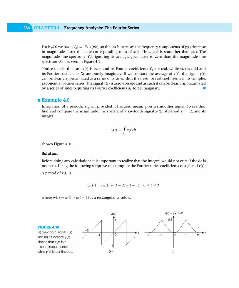
n Example 4.8Integration of a periodic signal, provided it has zero mean, gives a smoother signal. To see this,find and compare the magnitude line spectra of a sawtooth signal x(t), of period T0 = 2, and itsintegral

y(t) =∫

x(t)dt

shown Figure 4.10.

Solution

Before doing any calculations it is important to realize that the integral would not exist if the dc isnot zero. Using the following script we can compute the Fourier series coefficients of x(t) and y(t).

A period of x(t) is

x1(t) = tw(t)+ (t − 2)w(t − 1) 0 ≤ t ≤ 2

where w(t) = u(t)− u(t − 1) is a rectangular window.

FIGURE 4.10(a) Sawtooth signal x(t)and (b) its integral y(t).Notice that x(t) is adiscontinuous functionwhile y(t) is continuous. (a) (b)

x (t )

1−1

−20

1

−1

t

· · ·

· · ·

y (t ) = ∫ x (t )dt

−1−2t

0.5

0 1 2

·· · · · ·

4.7 Convergence of the Fourier Series 265

(a) (b)

0 0.5 1 1.5 2−1

−0.5

0

0.5

1

t

Period

x(t

)

0 20 40 600

0.1

0.2

0.3

0.4

Ω

|Xk|

|Xk|

0 20 40 60−2

−1

0

1

2

Ω

0 0.5 1 1.5 20

0.10.20.30.40.5

t

Period

y(t

)

|Xk|

0 20 40 600

1

2

3

4

Ω0 20 40 60

0

0.1

0.2

0.3

0.4

Ω

|Yk|

FIGURE 4.11(a) Periods of the sawtooth signal x(t) and (b) its integral y(t) and their magnitude and phase line spectra.

%%%%%%%%%%%%%%%%%% Example 4.8---Saw-tooth signal and its integral%%%%%%%%%%%%%%%%syms tT0 = 2;m = heaviside(t) − heaviside(t − T0/2);m1 = heaviside(t − T0/2) - heaviside(t − T0);x = t ∗ m + (t − 2) ∗ m1;y = int(x);[X, w] = fourierseries(x, T0, 20);[Y, w] = fourierseries(y, T0, 20);

The signal y(t) is smoother than x(t); y(t) is a continuous function of time, while x(t) isdiscontinuous. This is indicated as well by the magnitude line spectra of the two signals. Ignor-ing the dc components, the |Yk| of y(t) decay a lot faster to zero than the |Xk| of x(t) (SeeFigure 4.11). As we will see in Section 4.10, computing the derivative of a periodic signal is equiva-lent to multiplying its Fourier series coefficients by j0k, which emphasizes the higher harmonics.If the periodic signal is zero-mean so that its integral exists, the Fourier coefficients of the integralcan be found by dividing them by j0k so that now the low harmonics are emphasized. n

4.7 CONVERGENCE OF THE FOURIER SERIESIt can be said, without overstating it, that any periodic signal of practical interest has a Fourier series.Only very strange signals would not have a converging Fourier series. Establishing convergence isnecessary because the Fourier series has an infinite number of terms. To establish some general


conditions under which the series converges, we need to classify signals with respect to theirsmoothness.

A signal x(t) is said to be piecewise smooth if it has a finite number of discontinuities, while a smoothsignal has a derivative that changes continuously. Thus, smooth signals can be considered specialcases of piecewise smooth signals.

The Fourier series of a piecewise smooth (continuous or discontinuous) periodic signal x(t) converges for allvalues of t. The mathematician Dirichlet showed that for the Fourier series to converge to the periodic signalx(t), the signal should satisfy the following sufficient (not necessary) conditions over a period:

n Be absolutely integrable.n Have a finite number of maxima, minima, and discontinuities.

The infinite series equals x(t) at every continuity point and equals the average

0.5[x(t + 0+)+ x(t + 0−)]

of the right limit x(t + 0+) and the left limit x(t + 0−) at every discontinuity point. If x(t) is continuouseverywhere, then the series converges absolutely and uniformly.

Although the Fourier series converges to the arithmetic average at discontinuities, it can be observedthat there is some ringing before and after the discontinuity points. This is called the Gibb’s phe-nomenon. To understand this phenomenon it is necessary to explain how the Fourier series can beseen as an approximation to the actual signal, and how when a signal has discontinuities the conver-gence is not uniform around them. It will become clear that the smoother the signal x(t) is, the easierit is to approximate it with a Fourier series with a finite number of terms.

When the signal is continuous everywhere, the convergence is such that at each point t the seriesapproximates the actual value x(t) as we increase the number of terms in the approximation. How-ever, that is not the case when discontinuities occur in the signal. This is despite the fact that aminimum mean-square approximation seems to indicate that the approximation could give a zeroerror. Let

xN(t) =N∑

k=−N

Xkejk0t (4.24)

be the Nth-order approximation of a periodic signal x(t), of fundamental frequency 0, thatminimizes the average quadratic error over a period

EN =1T0

∫T0

|x(t)− xN(t)|2dt (4.25)


with respect to the Fourier coefficients Xk. To minimize EN with respect to the coefficients Xk we setits derivative with respect to Xk to zero. Let ε(t) = x(t)− xN(t), so that

dEN

dXk=

1T0

∫T0

2ε(t)dε∗(t)dXk

dt

= −1T0

∫T0

2[x(t)− xN(t)]e−jk0tdt

= 0

which after replacing xN(t) and using the orthogonality of the Fourier exponentials gives

Xk =1T0

∫T0

x(t)e−j0ktdt (4.26)

corresponding to the Fourier coefficients of x(t) for −N ≤ k ≤ N. As N→∞ the average errorEN → 0.

The only issue left is how xN(t) converges to x(t). As indicated before, if x(t) is smooth xN(t) approxi-mates x(t) at every point, but if there are discontinuities the approximation is in an average fashion.The Gibb’s phenomenon indicates that around discontinuities there will be ringing, regardless of theorder N of the approximation, even though the average quadratic error EN goes to zero as N increases.This phenomenon will be explained in Chapter 5 as the effect of using a rectangular window to obtaina finite-frequency representation of a periodic signal.

n Example 4.9To illustrate the Gibb’s phenomenon consider the approximation of a train of pulses x(t) withzero mean and period T0 = 1 (see the dashed signal in Figure 4.12) with a Fourier series xN(t)with N = 1, . . . , 20.

Solution

We compute analytically the Fourier coefficients of x(t) and use them to obtain an approxima-tion xN(t) of x(t) having a zero DC component and up to 20 harmonics. The dashed-line plot inFigure 4.12 is x(t) and the solid–line plot is xN(t) when N = 20. The discontinuities of the pulsetrain cause the Gibb’s phenomenon. Even if we increase the number of harmonics there is anovershoot in the approximation around the discontinuities.


FIGURE 4.12Approximate Fourier series xN(t) of the pulsetrain x(t) (discontinuous) using the DC componentand 20 harmonics. The approximate xN(t)displays the Gibb’s phenomenon around thediscontinuities.

0 0.2 0.4 0.6 0.8

−1

−0.5

0

0.5

1

x(t

), x

N(t

)

t (sec)

%%%%%%%%%%%%%%%%%% Example 4.9---Simulation of Gibb’s phenomenon%%%%%%%%%%%%%%%%clf; clear allw0 = 2 ∗ pi; DC = 0; N = 20; % parameters of periodic signal% computation of Fourier series coefficientsfor k = 1:N,

X(k) = sin(k ∗ pi/2)/(k ∗ pi/2);endX = [DC X]; % Fourier series coefficients% computation of periodic signalTs = 0.001; t = 0:Ts:1 − Ts;L = length(t); x = [ones(1, L/4) zeros(1, L/2) ones(1, L/4)]; x = x − 0.5;% computation of approximatexN = X(1)∗ones(1,length(t));for k = 2:N,

xN = xN + 2 ∗ X(k) ∗ cos(2 ∗ pi ∗ (k − 1). ∗ t); % approximate signalplot(t, xN); axis([0 max(t) 1.1 ∗ min(xN) 1.1 ∗ max(xN)])hold on; plot(t, x, ’r’)ylabel(’x(t), x N(t)’); xlabel(’t (sec)’);gridhold offpause(0.1)

end

When you execute the above script, it pauses to display the approximation for an increasing num-ber of terms in the approximation. At each of these values ringing around the discontinuities theGibb’s phenomenon is displayed. n


n Example 4.10Consider the mean-square error optimization to obtain an approximation of the periodic sig-nal x(t) shown in Figure 4.4 from Example 4.5. We wish to obtain an approximate x2(t) =α + 2β cos(0t), given that it is clear that x(t) has an average, and that once we subtract it from thesignal the resulting signal is approximated by a cosine function. Minimize the mean-square error

E2 =1T0

∫T0

|x(t)− x2(t)|2dt

with respect to α and β to find these values.

Solution

To minimize E2 we set to zero its derivatives with respect to α and β to get

dE2

dα= −

1T0

∫T0

2[x(t)− α − 2β cos(0t)]dt = −1T0

∫T0

2[x(t)− α]dt = 0

dE2

dβ= −

1T0

∫T0

2[x(t)− α − 2β cos(0t)] cos(0t)dt = 0

which, after getting rid of 2T0

of both sides of the above equations and applying the orthogonalityof the Fourier basis, gives

α =1T0

∫T0

x(t)dt

β =1T0

∫T0

x(t) cos(0t)dt

For the signal in Figure 4.4 we obtain

α = 1

β =2π

giving as approximation the signal

x2(t) = 1+4π

cos(2πt)

which at t = 0 gives x2(0) = 2.27 instead of the expected 2; x2(0.25) = 1 (because of thediscontinuity at this point, this value is the average of 2 and 0, the values, respectively, beforeand after the discontinuity) instead of 2 and x2(0.5) = −0.27 instead of the expected 0. n


n Example 4.11Consider the train of pulses in Example 4.5. Determine how many Fourier coefficients are necessaryto get a representation containing 97% of the power of the periodic signal.

Solution

The desired 97% of the power of x(t) is

0.971T0

∫T0

x2(t)dt = 0.97

0.25∫−0.25

4dt = 1.94

and so we need to find an integer N such that

N∑k=−N

|Xk|2=

N∑k=−N

∣∣∣∣ sin(πk/2)(πk/2)

∣∣∣∣2 = 1.94

The value of N is found by trial and error, adding consecutive values of the magnitude squaredof Fourier coefficients. Using MATLAB, it is found that for N = 5 (dc and 5 harmonics) theFourier series approximation has a power of 1.93. Thus, 11 Fourier coefficients give a very goodapproximation to the periodic train of pulses, with about 97% of the signal power. n

4.8 TIME AND FREQUENCY SHIFTINGTime shifting and frequency shifting are duals of each other.

n Time-shifting: A periodic signal x(t), of period T0, remains periodic of the same period when shifted intime. If Xk are the Fourier coefficients of x(t), the Fourier coefficients for x(t − t0) are

Xke−jk0t0 = |Xk|ej(∠Xk−k0t0)

(4.27)

That is, only a change in phase is caused by the time shift. The magnitude spectrum remains the same.

n Frequency-shifting: When a periodic signal x(t), of period T0, modulates a complex exponential ej1t :

n The modulated signal x(t)ej1t is periodic of period T0 if 1 = M0 for an integer M ≥ 1.n The Fourier coefficients Xk are shifted to frequencies k0 +1.n The modulated signal is real-valued by multiplying x(t) by cos(1t).

If we delay or advance in time a periodic signal, the resulting signal is periodic of the same period.Only a change in the phase of the coefficients occurs to accommodate for the shift. Indeed, if

x(t) =∑

k

Xkejk0t

4.8 Time and Frequency Shifting 271

we then have that

x(t − t0) =∑

k

Xkejk0(t−t0) =∑

k

[Xke−jk0t0

]ejk0t

x(t + t0) =∑

k

Xkejk0(t+t0) =∑

k

[Xkejk0t0

]ejk0t

so that the Fourier coefficients Xk corresponding to x(t) are changed to Xke∓jk0t0 forx(t ∓ t0). In both cases, they have the same magnitude |Xk| but different phases.

In a dual way, if we multiply the above periodic signal x(t) by a complex exponential of frequency1, ej1t, we obtain a so-called modulated signal y(t) and its spectrum is shifted in frequency by 1

with respect to the spectrum of the periodic signal x(t). In fact,

y(t) = x(t)ej1t

=

∑k

Xkej(0k+1)t

indicating that the harmonic frequencies are shifted by 1. The signal y(t) is not necessarily periodic.Since T0 is the period of x(t), then

y(t + T0) = x(t + T0)ej1(t+T0)

and for it to be equal to y(t), then 1T0 = 2πM, for an integer M 6= 0 or

1 = M0 M >> 1

which goes along with the condition that the modulating frequency 1 is chosen much larger than0. The modulated signal is then given by

y(t) =∑

k

Xkej(0k+1)t =∑

k

Xkej0(k+M)t=

∑`

X`−Mej0`t

so that the Fourier coefficients are shifted to new frequencies 0(k+M).

To keep the modulated signal real-valued, one multiplies the periodic signal x(t) by a cosine offrequency 1 = M0 for M >> 1 to obtain a modulated signal

y1(t) = x(t) cos(1t)

=

∑k

0.5Xk[ej(k0+1)t + ej(k0−1)t]

so that the harmonic components are now centered around ±1.


n Example 4.12To illustrate the modulation property using MATLAB consider modulating a sinusoid cos(20πt)with a train of square pulses

x1(t) = 0.5[1+ sign(sin(πt)]

and with a sinusoid

x2(t) = cos(πt)

Use our function fourierseries to find the Fourier series of the modulated signals and plot theirmagnitude line spectra.

Solution

The function sign is defined as

sign(x(t)) =−1 x(t) < 0

1 x(t) ≥ 0(4.28)

That is, it determines the sign of the signal. Thus, 0.5[1+ sign(sin(πt)] = u(t)− u(t − 1) equals

1 for 0 ≤ t ≤ 1, and 0 for 1 < t ≤ 2, which corresponds to a period of a train of squarepulses.

The following script allows us to compute the Fourier coefficients of the two modulated signals.

%%%%%%%%%%%%%%%%%% Example 4.12---Modulation%%%%%%%%%%%%%%%%syms tT0 = 2;m = heaviside(t) − heaviside(t − T0/2);m1 = heaviside(t) − heaviside(t − T0);x = m ∗ cos(20 ∗ pi ∗ t);x1 = m1 ∗ cos(pi ∗ t) ∗ cos(20 ∗ pi ∗ t);[X, w] = fourierseries(x, T0, 60);[X1, w1] = fourierseries(x1, T0, 60);

The modulated signals and their corresponding magnitude line spectra are shown in Figure 4.13.The Fourier coefficients of the modulated signals are now clustered around the frequency 20π .

4.9 Response of LTI Systems to Periodic Signals 273

FIGURE 4.13(a) Modulated square-wavex1(t) cos(20πt) and (b) cosinex2(t) cos(20πt) and theirrespective magnitude linespectra. (a) (b)

0 2 4

−1

−0.5

0

0.5

1

t

x 1(t

)

0 50 100 1500

0.1

0.2

Ω

|X1k

|

0 2 4

−1

−0.5

0

0.5

1

t

x 2(t

)

00 50 100 150

0.1

0.2

Ω

|X2k

|

n

4.9 RESPONSE OF LTI SYSTEMS TO PERIODIC SIGNALSThe most important property of LTI systems is the eigenfunction property.

Eigenfunction property : In steady state, the response to a complex exponential (or a sinusoid) of a certainfrequency is the same complex exponential (or sinusoid), but its amplitude and phase are affected by thefrequency response of the system at that frequency.

Suppose that the impulse response of an LTI system is h(t) and that H(s) = L[h(t)] is thecorresponding transfer function. If the input to this system is a periodic signal x(t), of period T0,with Fourier series

x(t) =∞∑

k=−∞

Xkejk0t 0 =2πT0

(4.29)

then according to the eigenfunction property the output in the steady state is

yss(t) =∞∑

k=−∞

[XkH( jk0)] ejk0t (4.30)


If we call Yk = XkH( jk0) we have a Fourier series representation of yss(t) with Yk as its Fouriercoefficients.

4.9.1 Sinusoidal Steady StateIf the input of a stable and causal LTI system, with impulse response h(t), is x(t) = Aej0t, theoutput is

y(t) =

∞∫0

h(τ )x(t − τ)dτ = Aej0t

∞∫0

h(τ )e−j0τdτ

= Aej0tH( j0) = A|H( j0)|ej0t+∠H( j0) (4.31)

The limits of the first integral indicate that the system is causal (the h(τ ) = 0 for τ < 0) and thatthe input x(t − τ) is applied from −∞ (when τ = ∞) to t (when τ = 0); thus y(t) is the steady-stateresponse of the system. If the input is a sinusoid—for example,

x1(t) = Re[x(t) = Aej0t] = A cos(0t) (4.32)

then the corresponding steady-state response is

y1(t) = Re[A|H( j0)|ej0t+∠H( j0)]

= A|H( j0)| cos(0t + ∠H( j0)). (4.33)

As in the eigenfunction property, the frequency of the output coincides with the frequency of theinput, however, the magnitude and the phase of the input signal is changed by the response of thesystem at the input frequency.

The following script simulates the convolution of a sinusoid x(t) of frequency = 20π , amplitude10, and random phase with the impulse response h(t) (a modulated decaying exponential) of an LTIsystem. The convolution integral is approximated using the MATLAB function conv.

%%%%%%%%%%%%%%%%%% Simulation of Convolution%%%%%%%%%%%%%%%%clear all; clfTs = 0.01; Tend = 2; t = 0:Ts:Tend;x = 10 ∗ cos(20 ∗ pi ∗ t + pi ∗ (rand(1, 1) − 0.5)); % input signalh = 20 ∗ exp(−10.ˆt). ∗ cos(40 ∗ pi ∗ t); % impulse response% approximate convolution integraly = Ts ∗ conv(x, h);


M = length(x);figure(1)x1 = [zeros(1, 5) x(1:M)];z = y(1); y1 = [zeros(1, 5) z zeros(1, M − 1)];t0 = −5 ∗ Ts:Ts:Tend;for k = 0:M − 6,

pause(0.05)h0 = fliplr(h);h1 = [h0(M - k - 5:M) zeros(1, M - k - 1)];subplot(211)plot(t0, h1, ’r’)hold onplot(t0, x1, ’k’)title(’Convolution of x(t) and h(t)’)ylabel(’x(τ ), h(t-τ )’); grid; axis([min(t0) max(t0) 1.1*min(x) 1.1*max(x)])hold off

subplot(212)plot(t0, y1, ’b’)ylabel(’y(t) = (x ∗ h)(t)’); grid; axis([min(t0) max(t0) 0.1 ∗ min(x) 0.1 ∗ max(x)])z = [z y(k + 2)];y1 = [zeros(1, 5) z zeros(1, M - length(z))];

end

Figure 4.14 displays the last step of the convolution integral simulation. Notice that the steady stateis attained in a very short time (around t = 0.5 sec). The transient changes every time that the scriptis executed due to the random phase.

FIGURE 4.14Convolution simulation: (a) input x(t) (solid line) andh(t − τ) (dashed line), and (b) output y(t): transientand steady-state response.

0 0.5 1

(a)

(b)

1.5 2−10

−5

0

5

10

x(τ

), h

(t−τ

)

τ

0 0.5 1 1.5 2

−0.5

0

0.5

y(t

)=(x

*h)(

t)

t


If the input x(t) of a causal and stable LTI system, with impulse response h(t), is periodic of period T0 and hasthe Fourier series

x(t) = X0 + 2∞∑

k=1

|Xk| cos(k0t +∠Xk) 0 =2πT0

(4.34)

the steady-state response of the system is

y(t) = X0|H( j0)| cos(∠H( j0))+ 2∞∑

k=1

|Xk||H( jk0)| cos(k0t +∠Xk +∠H( jk0)) (4.35)

where

H( jk0) =

∞∫0

h(τ )e−jk0τ dτ (4.36)

is the frequency response of the system at k0.

Remarks

n If the input signal x(t) is a combination of sinusoids of frequencies that are not harmonically related, thesignal is not periodic, but the eigenfunction property still holds. For instance, if

x(t) =∑

k

Ak cos(kt + θk)

and the frequency response of the LTI system is H( j), the steady-state response is

y(t) =∑

k

Ak|H( jk)| cos(kt + θk + ∠H( jk))

n It is important to realize that if the LTI system is represented by a differential equation and the inputis a sinusoid, or combination of sinusoids, it is not necessary to use the Laplace transform to obtain thecomplete response and then let t→∞ to find the sinusoidal steady-state response. The Laplace transformis only needed to find the transfer function of the system, which can then be used in Equation (4.35) tofind the sinusoidal steady state.

4.9.2 Filtering of Periodic SignalsAccording to Equation (4.35) if we know the frequency response of the system (Eq. 4.36), at theharmonic frequencies of the periodic input, H( jk0), we have that in the steady state the output ofthe system y(t) is as follows:

n Periodic of the same period as the input.n Its Fourier coefficients are those of the input Xk multiplied by the frequency response at the

harmonic frequencies, H( jk0).


n Example 4.13To illustrate the filtering of a periodic signal, consider a zero-mean pulse train

x(t) =∞∑

k=−∞,6=0

sin(kπ/2)kπ/2

ej2kπt

as the driving source of an RC circuit that realizes a low-pass filter (i.e., a system that tries tokeep the low-frequency harmonics and get rid of the high-frequency harmonics of the input). Thetransfer function of the RC low-pass filter is

H(s) =1

1+ s/100

Solution

The following script computes the frequency response of the filter at the harmonic frequenciesH( jk0) (see Figure 4.15).

%%%%%%%%%%%%%%%%%% Example 4.13%%%%%%%%%%%%%%%%% Freq response of H(s)=1/(s/scale+1) -- low-pass filterw0 = 2 * pi; % fundamental frequency of inputM = 20; k = 0:M - 1; w1 = k. * w0; % harmonic frequenciesH = 1./(1 + j * w1/100); Hm = abs(H); Ha = angle(H); % frequency responsesubplot(211)stem(w1, Hm, ’filled’); grid; ylabel(’—H(jω)—’)axis([0 max(w1) 0 1.3])subplot(212)stem(w1, Ha, ’filled’); gridaxis([0 max(w1) -1 0])ylabel(’¡H(j ω)’); xlabel(’w (rad/sec)’)

The response due to the pulse train can be found by finding the response to each of its Fourierseries components and adding them. Approximating x(t) using N = 20 harmonics by

xN(t) =20∑

k=−20,6=0

sin(kπ/2)kπ/2

ej2kπt

Then the output voltage across the capacitor is given in the steady state,

yss(t) =20∑

k=−20, 6=0

H( j2kπ)sin(kπ/2)

kπ/2ej2kπt


Because the magnitude response of the low-pass filter changes very little in the range of frequenciesof the input, the output signal is very much like the input (see Figure 4.15). The following script isused to find the response.

% low-pass filtering% FS coefficients of inputX(1) = 0; % mean valuefor k = 2:M - 1,

X(k) = sin((k − 1) ∗ pi/2)/((k − 1) ∗ pi/2);end% periodic signalTs = 0.001; t1 = 0:Ts:1 - Ts;L = length(t1);x1 = [ones(1, L /4) zeros(1, L /2) ones(1, L /4)]; x1 = x1 − 0.5; x = [x1 x1];% output of filtert = 0:Ts:2 − Ts;y = X(1) ∗ ones(1, length(t)) ∗ Ha(1);plot(t, y); axis([0 max(t) − .6 .6])for k = 2:M - 1,

y = y + X(k) ∗ Hm(k) ∗ cos(w0 ∗ (k − 1). ∗ t + Ha(k));plot(t, y); axis([0 max(t) − .6 .6]); hold onplot(t, x, ’r’); axis([0 max(t) − 0.6 0.6]); gridylabel(’x(t), y(t)’); xlabel(’t (sec)’) ; hold offpause(0.1)

end

(a) (b)

0 20 40 60 80 1000

0.5

1

|H(j

Ω)|

0 20 40 60 80 100−1

−0.5

0

<H(j

Ω)

Ω (rad/sec)0.2 0.4 0.6 0.8 1 1.2 1.4 1.6 1.8

−0.5−0.4−0.3−0.2−0.1

00.10.20.30.40.5

x(t

), y

(t)

t (sec)

FIGURE 4.15(a) Magnitude and phase response of the low-pass RC filter H(s) at harmonic frequencies, and (b) response dueto a train of pulses. n

4.10 Other Properties of the Fourier Series 279

4.10 OTHER PROPERTIES OF THE FOURIER SERIESIn this section we present additional properties of the Fourier series that will help us with its compu-tation and with our understanding of the relation between time and frequency. We are in particularinterested in showing that even and odd signals have special representations, and that it is possibleto find the Fourier series of the sum, product, derivative, and integral of periodic signals without theintegration required by the definition of the series.

4.10.1 Reflection and Even and Odd Periodic SignalsIf the Fourier series of x(t), periodic with fundamental frequency 0, is

x(t) =∑

k

Xkejk0t

then the one for its reflected version x(−t) is

x(−t) =∑m

Xme−jm0t=

∑k

X−kejk0t (4.37)

so that the Fourier coefficients of x(−t) are X−k (remember that m and k are just dummy variables).This can be used to simplify the computation of Fourier series of even and odd signals.

For an even signal x(t), we have that x(t) = x(−t), and as such Xk = X−k and therefore x(t) is naturallyrepresented in terms of cosines and a dc term. Indeed, its Fourier series is

x(t) = X0 +

−1∑k=−∞

Xkejkot+

∞∑k=1

Xkejkot

= X0 +

∞∑k=1

Xk[ejkot+ e−jkot]

= X0 + 2∞∑

k=1

Xk cos(k0t) (4.38)

indicating that Xk are real-valued. This is also seen from

Xk =1T0

∫T0

x(t)e−jk0tdt =1T0

∫T0

x(t)[cos(k0t)− j sin(k0)]dt

=1T0

∫T0

x(t) cos(k0t)dt

because x(t) sin(k0t) is odd and their integral is zero. It will be similar for an odd function for whichx(t) = −x(−t), or Xk = −X−k, in which case the Fourier series has a zero dc value and sine harmonics.


The Xk are purely imaginary. Indeed, for an odd x(t),

Xk =1T0

∫T0

x(t)e−jk0tdt =1T0

∫T0

x(t)[cos(k0t)− j sin(k0)]dt

=−jT0

∫T0

x(t) sin(k0t)dt

since x(t) cos(k0t) is odd. The Fourier series of an odd function can thus be written as

x(t) = 2∞∑

k=1

( jXk) sin(k0t) (4.39)

According to the even and odd decomposition, any periodic signal x(t) can be expressed as

x(t) = xe(t)+ xo(t)

where xe(t) is the even and xo(t) is the odd component of x(t). Finding the Fourier coefficients ofxe(t), which will be real, and those of xo(t), which will be purely imaginary, we would then haveXk = Xek + Xok since

xe(t) = 0.5[x(t)+ x(−t)] ⇒ Xek = 0.5[Xk + X−k]

xo(t) = 0.5[x(t)− x(−t)] ⇒ Xok = 0.5[Xk − X−k] (4.40)

n Reflection: If the Fourier coefficients of a periodic signal x(t) are Xk then those of x(−t), the time-reversedsignal with the same period as x(t), are X−k.

n Even periodic signal x(t): Its Fourier coefficients Xk are real, and its trigonometric Fourier series is

x(t) = X0 + 2∞∑

k=1

Xk cos(k0t) (4.41)

n Odd periodic signal x(t): Its Fourier coefficients Xk are imaginary, and its trigonometric Fourier series is

x(t) = 2∞∑

k=1

jXk sin(k0t) (4.42)

For any periodic signal x(t) = xe(t)+ xo(t) where xe(t) and xo(t) are the even and odd component of x(t), then

Xk = Xek + Xok (4.43)

where Xek are the Fourier coefficients of xe(t) and Xok are the Fourier coefficients of xo(t).

n Example 4.14Consider the periodic signals x(t) and y(t) shown in Figure 4.16. Determine their Fouriercoefficients by using the symmetry conditions and the even–odd decomposition.


FIGURE 4.16Nonsymmetric periodic signals.

2

1−1−2 0

0 1 2 3−2 −1

2

2 3t

t

· · ·· · ·

· · · · · ·

x (t )

y (t )

Solution

The given signal x(t) is neither even nor odd, but the advance signal x(t + 0.5) is even with a periodof T0 = 2, 0 = π . Then between −1 and 1 the shifted period is

x1(t + 0.5) = 2[u(t + 0.5)− u(t − 0.5)]

so that its Laplace transform is

X1(s)e0.5s=

2s

[e0.5s− e−0.5s

]which gives the Fourier coefficients

Xk =12

2jkπ

[ejkπ/2

− e−jkπ/2]

e−jkπ/2

=1

0.5πksin(0.5πk)e−jkπ/2

after replacing s by jko = jkπ and dividing by the period T0 = 2. These coefficients are complexas corresponding to a signal that is neither even nor odd. The dc coefficient is X0 = 1.

The given signal y(t) is neither even nor odd, and cannot be made even or odd by shifting. The evenand odd components of a period of y(t) are shown in Figure 4.17. The even and odd componentsof a period y1(t) between −1 and 1 are

y1e(t) = [u(t + 1)− u(t − 1)]︸︷︷︸rectangular pulse

+ [r(t + 1)− 2r(t)+ r(t − 1)]︸︷︷︸triangle

y1o(t) = t[u(t + 1)− u(t − 1)] = [(t + 1)u(t + 1)− u(t + 1)]− [(t − 1)u(t − 1)+ u(t − 1)]

= r(t + 1)− r(t − 1)− u(t + 1)− u(t − 1)


FIGURE 4.17Even and odd components of the period of y(t),−1 ≤ t ≤ 1.

t

y1e(t ) y1o(t )

1−1−1

−1

1

0

2

t1

1

Thus, the mean value of ye(t) is the area under y1e(t) divided by 2 or 1.5, and for k 6= 0,

Yek =1T0

Y1e(s)∣∣s=jk0 =

12

[1s(es− e−s)+

1s2 (e

s− 2+ e−s)

]s=jkπ

=sin(kπ)πk

+1− cos(kπ)(kπ)2

= 0+1− cos(kπ)(kπ)2

=1− (−1)k

(kπ)2

The mean value of yo(t) is zero, and for k 6= 0,

Yok =1T0

Y1o(s)∣∣s=jk0 =

12

[es− e−s

s2 −es+ e−s

s

]s=jkπ

= −jsin(kπ)(kπ)2

+ jcos(kπ)

kπ= 0+ j

cos(kπ)kπ

= j(−1)k

kπ

Finally, the Fourier series coefficients of y(t) are

Yk =

Ye0 + Yo0 = 1.5+ 0 = 1.5 k = 0Yek + Yok = (1− (−1)k)/(kπ)2 + j(−1)k/(kπ) k 6= 0

n

4.10.2 Linearity of Fourier Series—Addition of Periodic Signals

n Same fundamental frequency: If x(t) and y(t) are periodic signals with the same fundamental frequency0, then the Fourier series coefficients of z(t) = αx(t)+ βy(t) for constants α and β are

Zk = αXk + βYk (4.44)

where Xk and Yk are the Fourier coefficients of x(t) and y(t).n Different fundamental frequencies: If x(t) is periodic of period T1, and y(t) is periodic of period T2 such

that T2/T1 = N/M, for nondivisible integers N and M, then z(t) = αx(t)+ βy(t) is periodic of period


T0 = MT2 = NT1, and its Fourier coefficients are

Zk = αXk/N + βYk/M for integers k such that k/N, and k/M are integers (4.45)

where Xk and Yk are the Fourier coefficients of x(t) and y(t).

If x(t) and y(t) are periodic signals of the same period T0, the Fourier coefficients of z(t) = αx(t)+βy(t) (also periodic of period T0) are then Zk = αXk + βYk where Xk and Yk are the Fourier coefficientsof x(t) and y(t), respectively.

In general, if x(t) is periodic of period T1, and y(t) is periodic of period T2, their sum z(t) = αx(t)+βy(t) is periodic if the ratio T2/T1 is a rational number (i.e., T2/T1 = N/M for some nondivisibleintegers N and M). If so, the period of z(t) is T0 = MT2 = NT1. The fundamental frequency of z(t)would be 0 = 1/N = 2/M for 1 the fundamental frequency of x(t) and 2 the fundamentalfrequency of y(t). The Fourier series of z(t) is then

z(t) = αx(t)+ βy(t) = α∑

k

Xkej1kt+ β

∑m

Ymej2mt

= α∑

k

XkejN0kt+ β

∑m

YmejM0mt

= α∑

n=0,±N,±2N,...

Xn/Nej0nt+ β

∑`=0,±M,±2M,...

Y`/Mej0`t

Thus, the coefficients are

Zk = αXk/N + βYk/M

for integers k such that k/N and k/M are integers.

n Example 4.15Consider the sum z(t) of a periodic signal x(t) of period T1 = 2, with a periodic signal y(t) withperiod T2 = 0.2. Find the Fourier coefficients Zk of z(t) in terms of the Fourier coefficients Xk andYk of x(t) and y(t).

Solution

The ratio T2/T1 = 1/10 = N/M is rational, so z(t) is periodic of period T0 = T1 = 10T2 = 2.The fundamental frequency of z(t) is 0 = 1 = π , and 2 = 100 = 10π is the fundamentalfrequency of y(t). Thus, the Fourier coefficients of z(t) are

Zk =

Xk + Yk/10 when k = 0,±10,±20, . . .Xk otherwise

n


4.10.3 Multiplication of Periodic Signals

If x(t) and y(t) are periodic signals of same period T0, then their product

z(t) = x(t)y(t) (4.46)

is also periodic of period T0, and with Fourier coefficients that are the convolution sum of the Fouriercoefficients of x(t) and y(t):

Zk =∑`

X`Yk−` (4.47)

If x(t) and y(t) are periodic with the same period T0, then z(t) = x(t)y(t) is also periodic of period T0,since z(t + kT0) = x(t + kT0)y(t + kT0) = x(t)y(t) = z(t). Furthermore,

x(t)y(t) =∑

k

Xkejk0t∑`

Y`ej`0t=

∑k

∑`

XkY`ej(k+`)0t

=

∑m

[∑k

XkYm−k

]ejm0t

= z(t)

where we let m = k+ `. The coefficients of the Fourier series of z(t) are then

Zm =∑

k

XkYm−k

or the convolution sum of the sequences Xk and Yk, to be formally defined in Chapter 8.

n Example 4.16Consider the train of rectangular pulses x(t) shown in Figure 4.4. Let z(t) = 0.25x2(t). Use theFourier series of z(t) to show that

Xk = α∑m

XmXk−m

for some constant α. Determine α.

Solution

The signal 0.5x(t) is a train of pulses of unit amplitude, so that z(t) = (0.5x(t))2 = 0.5x(t). Thus,Zk = 0.5Xk, but also as a product of 0.5x(t) with itself we have that

Zk =∑m

[0.5Xm][0.5Xk−m]


and thus

0.5Xk︸︷︷︸Zk

= 0.25∑m

XmXk−m ⇒ Xk =12

∑m

XmXk−m (4.48)

so that α = 0.5.

The Fourier series of z(t) = 0.5x(t) according to the results in Example 4.5 is

z(t) = 0.5x(t) =∞∑

k=−∞

sin(πk/2)πk

ejk2πt

If we define

S(k) = 0.5Xk =sin(kπ/2)

kπ⇒ Xk = 2S(k)

we have from Equation (4.48) the interesting result

S(k) =∞∑

m=−∞

S(m)S(k−m)

or the convolution sum of the discrete sinc function S(k) with itself is S(k). n

4.10.4 Derivatives and Integrals of Periodic Signals

n Derivative: The derivative dx(t)/dt of a periodic signal x(t), of period T0, is periodic of the same period T0.If Xk are the coefficients of the Fourier series of x(t), the Fourier coefficients of dx(t)/dt are

jk0Xk (4.49)

where 0 is the fundamental frequency of x(t).n Integral: For a zero-mean, periodic signal y(t), of period T0, the integral

z(t) =

t∫−∞

y(τ )dτ

is periodic of the same period as y(t), with Fourier coefficients

Zk =Yk

jk0k 6= 0

Z0 = −∑m 6=0

Ym1

jm00 =

2πT0

(4.50)

These properties come naturally from the Fourier series representation of the periodic signal. Oncewe find the Fourier series of a periodic signal, we can differentiate it or integrate it (only when the dc


value is zero). The derivative of a periodic signal is obtained by computing the derivative of each ofthe terms of its Fourier series—that is, if

x(t) =∑

k

Xkejk0t

then

dx(t)dt=

∑k

Xkdejk0t

dt=

∑k

[ jk0Xk] ejk0t

indicating that if the Fourier coefficients of x(t) are Xk, the Fourier coefficients of dx(t)/dt arejk0Xk.

To obtain the integral property we assume y(t) is a zero-mean signal so that its integral z(t) is finite.If for some integer M, MT0 ≤ t < (M+ 1)T0, then

z(t) =

t∫−∞

y(τ )dτ =

MT0∫−∞

y(τ )dτ +

t∫MT0

y(τ )dτ

= 0+

t∫MT0

y(τ )dτ

Replacing y(t) by its Fourier series gives

z(t) =

t∫MT0

y(τ )dτ =

t∫MT0

∑k6=0

Ykejk0τdτ

=

∑k 6=0

Yk

t∫MT0

ejk0τdτ =∑k6=0

Yk1

jk0

[ejk0t

− 1]

= −

∑k 6=0

Yk1

jk0+

∑k6=0

Yk1

jk0ejk0t

where the first term corresponds to the average Z0 and Zk = Yk/( jk0), k 6= 0, are the rest of theFourier coefficients of z(t).

Remarks It should be now clear why the derivative of a periodic signal x(t) enhances its higher harmonics.Indeed, the Fourier coefficients of the derivative dx(t)/dt are those of x(t), Xk, multiplied by j0k, whichincreases with k. Likewise, the integration of a zero-mean periodic signal x(t) does the opposite—that is, itmakes the signal smoother, as we multiply Xk by decreasing terms 1/( jk0) as k increases.


n Example 4.17Let g(t) be the derivative of a triangular train of pulses f (t), of period T0 = 1. The period of f (t),0 ≤ t ≤ 1, is

f1(t) = 2r(t)− 4r(t − 0.5)+ 2r(t − 1)

Use the Fourier series of g(t) to find the Fourier series of f (t).

Solution

According to the derivative property we have that

Fk =Gk

jk0k 6= 0

are the Fourier coefficients of f (t). The signal g(t) = df (t)/dt has a corresponding period g1(t) =df1(t)/dt = 2u(t)− 4u(t − 0.5)+ 2u(t − 1). The Fourier series coefficients of g(t) are

Gk =2e−0.5s

s

(e0.5s− 2+ e−0.5s

)|s=j2πk = 2(−1)k

cos(πk)− 1jπk

k 6= 0

which are used to obtain the coefficients Fk for k 6= 0. The dc component of f (t) is found to be 0.5from its plot as g(t) does not provide it. n

n Example 4.18Consider the reverse of Example 4.17. That is, given the periodic signal g(t) of period T0 = 1 andFourier coefficients

Gk = 2(−1)kcos(πk)− 1

jπkk 6= 0

and G0 = 0. Find the integral

z(t) =

t∫−∞

g(τ )dτ

Solution

As shown above, z(t) is also periodic of the same period as g(t) (i.e., T0 = 1). The Fouriercoefficients of z(t) are

Zk =Gk

j0k= (−1)k

4(cos(πk)− 1)( j2πk)2

= (−1)(k+1) cos(πk)− 1π2k2 k 6= 0


FIGURE 4.18Two periods of the approximate triangular signalxN(t) using 100 harmonics.

0 0.5 1 1.5 2

0

0.2

0.4

0.6

0.8

1

x N(t

)

t (sec)

and the average term is

Z0 = −∑m 6=0

Gm1

j2mπ=

∑m 6=0

(−1)mcos(πm)− 1(πm)2

= 0.5∞∑

m=−∞,m 6=0

(−1)m+1[

sin(πm/2)(πm/2)

]2

where we used 1− cos(πm) = 2 sin2(πm/2). We used the following script to obtain the average,and to approximate the triangular signal using 100 harmonics (see Figure 4.18). The mean isobtained as 0.498.

%%%%%%%%%%%%%%%%%% Example 4.18%%%%%%%%%%%%%%%%clf; clear allw0 = 2 * pi; N = 100; % parameters of periodic signal% computation of mean valueDC = 0;for m = 1:N,

DC = DC + 2 * (-1) ˆ (m) * (cos(pi * m) -1)/(pi * m) ˆ 2;end% computation of Fourier series coefficientsTs = 0.001; t = 0:Ts:2 - Ts;for k = 1:N,

X(k) = (-1)ˆ(k + 1)*(cos(pi * k) - 1)/((pi * k)ˆ2);endX = [DC X]; % Fourier series coefficientsxa = X(1)*ones(1,length(t));figure(1)

4.11 What Have We Accomplished? Where Do We Go from Here? 289

for k = 2:N,xa = xa + 2 * abs(X(k)) * cos(w0 * (k - 1). * t + angle(X(k))); % approximate signal

end n

4.11 WHAT HAVE WE ACCOMPLISHED? WHERE DO WE GO FROMHERE?

Periodic signals are not to be found in practice, so where did Fourier get the intuition to come up witha representation for them? As you will see, the fact that periodic signals are not found in practice doesnot mean that they are not useful. The Fourier representation of periodic signals will be fundamentalin finding a representation for nonperiodic signals.

A very important concept you have learned in this chapter is that the inverse relation between timeand frequency provides complementary information for the signal. The frequency domain consti-tutes the other side of the coin in representing signals. As mentioned before, it is the eigenfunctionproperty of linear time-invariant systems that holds the theory together. It will provide the funda-mental principle for filtering. You should have started to experience deja vu in terms of the propertiesof the Fourier series; some look like a version of the ones in the Laplace transform. This is due tothe connection existing between these transforms. You should have also noticed the usefulness of theLaplace transform in finding the Fourier coefficients, avoiding integration whenever possible. Table4.1 provides the basic properties of the Fourier series for continuous–time periodic signals.

Chapter 5 will extend some of the results obtained in this chapter, thus unifying the treatment ofperiodic and nonperiodic signals and the concept of spectrum. Also the frequency representation of

Table 4.1 Basic Properties of Fourier Series

Time Domain Frequency Domain

Signals and constants x(t), y(t) periodic Xk, Yk

with period T0,α,β

Linearity αx(t)+ βy(t) αXk + βYk

Parseval’s power relation Px =1T0

∫T0|x(t)|2dt Px =

∑k |Xk|

2

Differentiationdx(t)

dtjk0Xk

Integration∫ t−∞

x(t′)dt′ only if X0 = 0Xk

jk0k 6= 0,−

∑m6=0

Xm

jm0, dc

Time shifting x(t − α) e−jα0 Xk

Frequency shifting ejM0tx(t) Xk−M

Symmetry x(t) real |Xk| = |X−k| even

function of k

∠Xk = −∠X−k odd

function of k


systems will be introduced and exemplified by its application in filtering. Modulation is the basictool in communications and can be easily explained in the frequency domain.

PROBLEMS

4.1. Eigenfunctions and LTI systemsThe eigenfunction property is only valid for LTI systems. Consider the cases of nonlinear and of time-varying systems.(a) A system represented by the following input–output equation is nonlinear:

y(t) = x2(t)

Let x(t) = ejπt/4. Find the corresponding system output y(t). Does the eigenfunction property hold?Explain.

(b) Consider a time-varying system

y(t) = x(t)[u(t)− u(t − 1)]

Let x(t) = ejπt/4. Find the corresponding system output y(t). Does the eigenfunction property hold?Explain.

4.2. Eigenfunctions and LTI systemsThe output of an LTI system is

y(t) =

t∫0

h(τ )x(t − τ)dτ

where the input x(t) and the impulse response h(t) of the system are assumed to be causal. Let x(t) =2 cos(2πt)u(t). Compute the output y(t) in the steady state and determine if the eigenfunction propertyholds.

4.3. Eigenfunctions and frequency response of LTI systemsThe input–output equation for an analog averager is

y(t) =1T

t∫t−T

x(τ )dτ

Let x(t) = ej0t . Since the system is LTI, then the output should be

y(t) = ej0tH( j0)(a) Find y(t) for the given input and then compare it with the above equation to find H( j0), the response

of the averager at frequency 0.(b) Find H(s) and verify the frequency response value H( j0) obtained above.

4.4. Generality of eigenfunctionsThe eigenfunction property holds for any input signal, periodic or not, that can be expressed in sinusoidalform.(a) Consider the input x(t) = cos(t)+ cos(2πt), −∞ < t <∞, into an LTI system. Is x(t) periodic? If so,

indicate its period.

Problems 291

(b) Suppose that the system is represented by a first-order differential equation,

y′(t)+ 5y(t) = x(t)

where y(t) is the output of the system and the given x(t) is the input of the system. Find the steady-state response y(t) due to x(t) using the eigenfunction property.

4.5. Steady state of LTI systemsThe transfer function of an LTI system is

H(s) =Y(s)X(s)=

s+ 1

s2 + 3s+ 2

If the input to this system is x(t) = 1+ cos(t + π/4), −∞ < t <∞, what is the output y(t) in the steadystate?

4.6. Eigenfunction property of LTI systems and LaplaceThe transfer function of an LTI system is given by

H(s) =Y(s)X(s)=

1

s2 + 3s+ 2

and its input is

x(t) = 4u(t)

(a) Use the eigenfunction property of LTI systems to find the steady-state response y(t) of this system.(b) Verify your result in (a) by means of the Laplace transform.

4.7. Different ways to compute the Fourier coefficients—MATLABWe would like to find the Fourier series of a sawtooth periodic signal x(t) of period T0 = 1. The period ofx(t) is

x1(t) = r(t)[u(t)− u(t − 1)]

(a) Carefully plot x(t) and compute the Fourier coefficients Xk using the integral definition.(b) An easier way to do this is to use the Laplace transform of x1(t). Find Xk this way.(c) Use MATLAB to plot the signal x(t) and its magnitude and phase line spectra.(d) Obtain a trigonometric Fourier series x(t) consisting of the DC term and 40 harmonics to approximate

x(t). Use MATLAB to find the values of x(t) for t = 0 to 10 in steps of 0.001. How does it compare withx(t)?

4.8. Addition of periodic signals—MATLABConsider a sawtooth signal x(t) with period T0 = 2 and period

x1(t) =

t 0 ≤ t < 10 otherwise

(a) Find the Fourier coefficients Xk using the Laplace transform. Consider the cases when k is odd andeven (k 6= 0). You need to compute X0 directly from the signal.

(b) Let y(t) = x(−t). Find the Fourier coefficients Yk.(c) The sum z(t) = x(t)+ y(t) is a triangular function. Find the Fourier coefficients Zk and compare them

to Xk + Yk.(d) Use MATLAB to plot x(t), y(t), and z(t) and their corresponding magnitude line spectra. Find an

approximate of z(t) using the dc value and10 harmonics and plot it.


4.9. Fourier series coefficients via Laplace—MATLABThe computation of the Fourier series coefficients is simplified by the relation between the formula forthese coefficients and the Laplace transform of a period of the periodic signal.(a) A periodic signal x(t), of period T0 = 2 sec, has as period with the signal x1(t) = u(t)− u(t − 1), so

that x(t) can be represented as

x(t) =∞∑

m=−∞

x1(t −mT0)

Expand this sum, and use the information for x1(t) and T0 to carefully plot the periodic signal x(t).(b) Find the Laplace transform of x1(t), and let s = jk0, where0 = 2π/T0 is the fundamental frequency,

to obtain the Fourier coefficients of x(t).(c) Use MATLAB to plot the magnitude line spectrum of x(t). Find an approximate of x(t) using the dc

and 40 harmonics. Plot it.

4.10. Half- and full-wave rectifying and Fourier—MATLABRectifying a sinusoid provides a way to create a dc source. In this problem we consider the Fourier seriesof the full- and half-wave rectified signals. The full-wave rectified signal xf (t) has a period T0 = 1 and itsperiod from 0 to 1 is

x1(t) = sin(πt) 0 ≤ t ≤ 1

while the period for the half-wave rectifier signal xh(t) is

x2(t) =

sin(πt) 0 ≤ t ≤ 10 1 < t ≤ 2

with period T1 = 2.(a) Obtain the Fourier coefficients for both of these periodic signals.(b) Use the even and odd decomposition of xh(t) to obtain its Fourier coefficients. This computation of

the Fourier coefficients of xh(t) avoids some difficulties when you attempt to plot its magnitude linespectrum. Use MATLAB and your analytic results here to plot the magnitude line spectrum of thehalf-wave signal and use the dc and 40 harmonics to obtain an approximation of the half-wave signal.

4.11. Smoothness and Fourier series—MATLABThe smoothness of a period determines the way the magnitude line spectrum decays. Consider thefollowing periodic signals x(t) and y(t), both of period T0 = 2 sec, and with a period from 0 ≤ t ≤ T0equal to

x1(t) = u(t)− u(t − 1)

y1(t) = r(t)− 2r(t − 1)+ r(t − 2)

Find the Fourier series coefficients of x(t) and y(t) and use MATLAB to plot their magnitude line spectrumfor k = 0,±1,±2, . . . ,±20. Determine which of these spectra decays faster and how it relates to thesmoothness of the period. (To see this relate |Xk| to the corresponding |Yk|.)

4.12. Time support and frequency content—MATLABThe support of a period of a periodic signal relates inversely to the support of the line spectrum. Considertwo periodic signals: x(t) of period T0 = 2 and y(t) of period T1 = 1, and with periods

x1(t) = u(t)− u(t − 1) 0 ≤ t ≤ 2

y1(t) = u(t)− u(t − 0.5) 0 ≤ t ≤ 1

Problems 293

(a) Find the Fourier series coefficients for x(t) and y(t).(b) Use MATLAB to plot the magnitude line spectra of the two signals from 0 to 40π rad/sec. Plot them on

the same figure so you can determine which has a broader support. Indicate which signal is smootherand explain how it relates to its line spectrum.

4.13. Derivatives and Fourier SeriesGiven the Fourier series representation for a periodic signal,

x(t) =∞∑

k=−∞

Xkejk0t

we can compute derivatives of it, just like for any other signal.(a) Consider the periodic train of pulses shown in Figure 4.19. Compute its derivative

y(t) =dx(t)

dt

and carefully plot it. Find the Fourier series of y(t).(b) Use the Fourier series representation of x(t) and find its derivative to obtain the Fourier series of y(t).

How does it compare to the Fourier series obtained above?

4.14. Fourier series of sampling deltaThe periodic signal

δTs(t) =∞∑

m=−∞

δ(t −mTs)

will be very useful in the sampling of continuous-time signals.(a) Find the Fourier series of this signal—that is,

δTs(t) =∞∑

k=−∞

1kejkst

find the Fourier coefficients 1k.(b) Plot the magnitude line spectrum of this signal.(c) Plot δTs(t) and its corresponding line spectrum 1k as functions of time and frequency. Are they both

periodic? How are their periods related? Explain.

FIGURE 4.19Problem 4.13: train ofrectangular pulses.

· · · · · ·

2

x(t)

−0.25−0.75 0.750.25 1.25−1.25t

T0 = 1


4.15. Figuring out Fourier’s ideaFourier proposed to represent a periodic signal as a sum of sinusoids, perhaps an infinite number ofthem. For instance, consider the representation of a periodic signal x(t) as a sum of cosines of differentfrequencies

x(t) =∞∑

k=0

Ak cos(kt + θk)

(a) If x(t) is periodic of period T0, what should the frequencies k be?(b) Consider x(t) = 2+ cos(2πt)− 3 cos(6πt + π/4). Is this signal periodic? If so, what is its period T0?

Determine its trigonometric Fourier series as given above by specifying the values of Ak and θk for allvalues of k = 0, 1, . . ..

(c) Let the signal x1(t) = 2+ cos(2πt)− 3 cos(20t + π/4) (this signal is almost like x(t) given above,except that the frequency 6π rad/sec of the second cosine has been approximated by 20 rad/sec).Is this signal periodic? Can you determine its Fourier series as given above by specifying the valuesof Ak and θk for all values of k = 0, 1, . . .? Explain.

4.16. DC output from a full-wave rectified signal—MATLABConsider a full-wave rectifier that has as output a periodic signal x(t) of period T0 = 1 and a period of it isgiven as

x1(t) =

cos(πt) −0.5 ≤ t ≤ 0.50 otherwise

(a) Obtain the Fourier coefficients Xk.(b) Suppose we pass x(t) through an ideal filter of transfer function H(s). Determine the values of this

filter at harmonic frequencies 2πk, = 0,±1,±2, . . ., so that its output is a constant (i.e., we have a dcsource).

(c) Use MATLAB to plot the signal x(t) and its magnitude line spectrum.

4.17. Fourier series of sum of periodic signalsSuppose you have the Fourier series of two periodic signals x(t) and y(t) of periods T1 and T2, respectively.Let Xk and Yk be the Fourier series coefficients corresponding to x(t) and y(t).(a) If T1 = T2, what would be the Fourier series coefficients of z(t) = x(t)+ y(t) in terms of Xk

and Yk?(b) If T1 = 2T2, determine the Fourier series coefficients of w(t) = x(t)+ y(t) in terms of Xk and Yk?

4.18. Manipulation of periodic signalsLet the following be the Fourier series of a periodic signal x(t) of period T0 (fundamental frequency 0 =

2π/T0):

x(t) =∞∑

k=−∞

Xkej0kt

Consider the following functions of x(t), and determine if they are periodic and what are their periodsif so:n y(t) = 2x(t)− 3n z(t) = x(t − 2)+ x(t)n w(t) = x(2t)Express the Fourier series coefficients Yk, Zk, and Wk in terms of Xk.

Problems 295

4.19. Using properties to find the Fourier seriesUse the Fourier series of a square train of pulses (done in this chapter) to compute the Fourier series of thetriangular signal x(t) with a period,

x1(t) = r(t)− 2r(t − 1)+ r(t − 2)

(a) Find the derivative of x(t) or y(t) = dx(t)/dt and carefully plot it. Plot also z(t) = y(t)+ 1. Use theFourier series of the square train of pulses to compute the Fourier series coefficients of y(t) and z(t).

(a) Obtain the trigonometric Fourier series of y(t) and z(t) and explain why they are represented by sinesand why z(t) has a nonzero mean.

(c) Obtain the Fourier series coefficients of x(t) from those of y(t).(d) Obtain the sinusoidal form of x(t) and explain why the cosine representation is more appropriate for

this signal than a sine representation.

4.20. Applying Parseval’s result—MATLABWe wish to approximate the triangular signal x(t) in Problem 4.19 by its Fourier series with a finite numberof terms, let’s say 2N. This approximation should have 95% of the average power of the triangular signal.Use MATLAB to find the value of N.

4.21. Fourier series of multiplication of periodic signalsConsider the Fourier series of two periodic signals,

x(t) =∞∑

k=−∞

Xkejokt

y(t) =∞∑

k=−∞

Ykej1kt

(a) Let 1 = 0. Is z(t) = x(t)y(t) periodic? If so, what is its period and its Fourier series coefficients?(b) If 1 = 20. Is w(t) = x(t)y(t) periodic? If so, what is its period and its Fourier series coefficients?

4.22. Integration of periodic signalsConsider now the integral of the Fourier series of the pulse signal p(t) = x(t)− 1 of period T0 = 1, wherex(t) is given in Figure 4.20.

FIGURE 4.20Problem 4.23: train ofrectangular pulses.

· · · · · ·

2

x(t)

−0.25−0.75 0.750.25 1.25−1.25t

T0 = 1


(a) Given that an integral of p(t) is the area under the curve, find and plot the function

s(t) =

t∫−∞

p(t)dt t ≤ 1

Indicate the values of s(t) for t = 0, 0.25, 0.5, 0.75, and 1.(b) Find the Fourier series of p(t) and s(t) and relate their Fourier series coefficients.(c) Suppose you want to compute the integral

T0/2∫−T0/2

p(t)dt

using the Fourier series of p(t). What is the integral equal to?(d) You can also compute the integral from the plot of p(t):

T0/2∫−T0/2

p(t)dt

What is it? Does it coincide with the result obtained using the Fourier series? Explain.

4.23. Full-wave rectifying and DC sourcesLet x(t) = sin2(2πt), a periodic signal of period T0 = 1, and y(t) = | sin(2πt)|, which is also periodic ofperiod T1 = 0.5.(a) A trigonometric identity gives that

x(t) =12

[1− cos(4πt)]

Use this result to find its complex exponential Fourier series.(b) Use the Laplace transform to find the Fourier series of y(t).(c) Are x(t) and y(t) identical? Explain.(d) Indicate how you would use an ideal low-pass filter to get a DC source of unit value from x(t) and

y(t). Indicate the bandwidth and the magnitude of the filters. Compare these two signals in terms ofadvantages or disadvantages in generating the desired DC source.

4.24. Windowing and music sounds—MATLABIn the computer generation of musical sounds, pure tones need to be windowed to make them moreinteresting. Windowing mimics the way a musician would approach the generation of a certain sound.Increasing the richness of the harmonic frequencies is the result of the windowing, as we will see in thisproblem. Consider the generation of a musical note with frequencies around fA = 880 Hz. Assume our“musician” while playing this note uses three strokes corresponding to a window w1(t) = r(t)− r(t −T1)− r(t − T2)+ r(t − T0), so that the resulting sound would be the multiplication, or windowing, of apure sinusoid cos(2π fAt) by a periodic signal w(t), with w1(t) a period that repeats every T0 = 5T whereT is the period of the sinusoid. Let T1 = T0/4 and T2 = 3T0/4.(a) Analytically determine the Fourier series of the window w(t) and plot its line spectrum using MATLAB.

Indicate how you would choose the number of harmonics needed to obtain a good approximation tow(t).

(b) Use the modulation or the convolution properties of the Fourier series to obtain the coefficients of theproduct s(t) = cos(2π fAt)w(t). Use MATLAB to plot the line spectrum of this periodic signal and againdetermine how many harmonic frequencies you would need to obtain a good approximation to s(t).

Problems 297

(c) The line spectrum of the pure tone p(t) = cos(2π fAt) only displays one harmonic, the onecorresponding to the fA = 880 Hz frequency. How many more harmonics does s(t) have? To listento the richness in harmonics use the MATLAB function sound to play the sinusoid p(t) and s(t) (useFs = 2× 880 Hz to play both).

(d) Consider a combination of notes in a certain scale; for instance, let

p(t) = sin(2π × 440t)+ sin(2π × 550t)+ sin(2π × 660t)

Use the same windowing w(t), and let s(t) = p(t)w(t). Use MATLAB to plot p(t) and s(t) and tocompute and plot their corresponding line spectra. Use sound to play p(nTs) and s(nTs) usingFs = 1000.

4.25. Computation of π—MATLABAs you know, π is an irrational number that can only be approximated by a number with a finite numberof decimals. How to compute this value recursively is a problem of theoretical interest. In this problem weshow that the Fourier series can provide that formulation.(a) Consider a train of rectangular pulses x(t), with a period

x1(t) = 2[u(t + 0.25)− u(t − 0.25)]− 1 −0.5 ≤ t ≤ 0.5

and period T0 = 1. Plot the periodic signal and find its trigonometric Fourier series.(b) Use the above Fourier series to find an infinite sum for π .(c) If πN is an approximation of the infinite sum with N coefficients, and π is the value given by MATLAB,

find the value of N so that πN is 95% of the value of π given by MATLAB.

4.26. Square error approximation of periodic signals—MATLABTo understand the Fourier series consider a more general problem, where a periodic signal x(t), of periodT0, is approximated as a finite sum of terms,

x(t) =N∑

k=−N

Xkφk(t)

where φk(t) are orthonormal functions. To pose the problem as an optimization problem, consider thesquare error

ε =

∫T0

|x(t)− x(t)|2dt

and look for the coefficients X(k) that minimize ε.(a) Assume that x(t) as well as x(t) are real valued, and that x(t) is even so that the Fourier series

coefficients Xk are real. Show that the error can be expressed as

ε =

∫T0

x2(t)dt − 2N∑

k=−N

Xk

∫T0

x(t)φk(t)dt +N∑

`=−N

|X`|2T0

(b) Compute the derivative of ε with respect to Xn and set it to zero to minimize the error. Find Xn.(c) In the Fourier series the φk(t) are the complex exponentials and the Xn coincide with the Fourier

series coefficients. To illustrate the above procedure consider the case of the pulse signal x(t), of periodT0 = 1, and a period

x1(t) = 2[u(t + 0.25)− u(t − 0.25)]


Use MATLAB to compute and plot the approximation x(t) and the errror ε for increasing values of Nfrom 1 to 100.

(d) Concentrate your plot of x(t) around the one of the discontinuities, and observe the Gibb’s phe-nomenon. Does it disappear when N is very large. Plot x(t) around the discontinuity for N =1000.

4.27. Walsh functions—MATLABAs seen in Problem 4.26, the Fourier series is one of a possible class of representations in terms of orthonor-mal functions. Consider the case of the Walsh functions, which are a set of rectangular pulse signals thatare orthonormal in a finite time interval [0, 1]. These functions are such that: (1) they take only 1 and −1values, (2) φk(0) = 1 for all k, and (3) they are ordered according to the number of sign changes.(a) Consider obtaining the functions φkk=0, . . . ,5. The Walsh functions are clearly normal since when

squared they are unity for t ∈ [0, 1]. Let φ0(t) = 1 for t ∈ [0, 1] and zero elsewhere. Obtain φ1(t) withone change of sign and that is orthogonal to φ0(t). Find then φ2(t), which has two changes of signand is orthogonal to both φ0(t) and φ1(t). Continue this process. Carefully plot the φi(t), i = 0, . . . , 5.Use the MATLAB function stairs to plot these Walsh functions.

(b) Consider the Walsh functions obtained above as sequences of 1s and −1s of length 8, and care-fully write these six sequences. Observe the symmetry of the sequences corresponding to φi(t), i =0, 1, 3, 5, and determine the circular shift needed to find the sequence corresponding to φ2(t) fromthe sequence from φ1(t), and φ4(t) from φ3(t). Write a MATLAB script that generates a matrix8withentries as the sequences. Find the product (1/8)88T , and explain how this result connects with theorthonormality of the Walsh functions.

(c) We wish to approximate a ramp function x(t) = r(t), 0 ≤ t ≤ 1, using φkk=0, . . . ,5. This could bewritten as

r = 8a

where r is a vector of x(nT) = r(nT) where T = 1/8, a are the coefficients of the expansion, and 8 isthe Walsh matrix found above. Determine the vector a and use it to obtain an approximation of x(t).Plot x(t) and the approximation x(t) (use stairs for this signal).

frequency analysis: the fourier series · responds to the fourier transform of the convolution...

Documents