22.058 - lecture 4, convolution and fourier convolution convolution fourier convolution outline ...
TRANSCRIPT
22.058 - lecture 4, Convolution and Fourier Convolution
Convolution
Fourier Convolution
Outline Review linear imaging model Instrument response function vs Point spread function Convolution integrals• Fourier Convolution• Reciprocal space and the Modulation transfer function Optical transfer function Examples of convolutions Fourier filtering Deconvolution Example from imaging lab• Optimal inverse filters and noise
22.058 - lecture 4, Convolution and Fourier Convolution
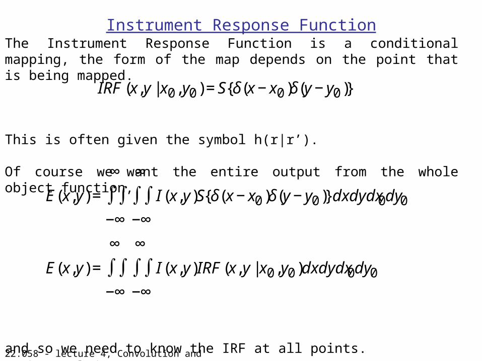
Instrument Response FunctionThe Instrument Response Function is a conditional mapping, the form of the map depends on the point that is being mapped.
This is often given the symbol h(r|r’).
Of course we want the entire output from the whole object function,
and so we need to know the IRF at all points.
€
IRF(x,y|x0,y0)=S δ(x−x0)δ(y−y0){ }
€
E(x,y)=
∞
∫∫−∞
∞
∫∫−∞
I (x,y)S δ(x−x0)δ(y−y0){ }dxdydx0dy0
E(x,y)=
∞
∫∫−∞
∞
∫∫−∞
I (x,y)IRF(x,y|x0,y0)dxdydx0dy0
22.058 - lecture 4, Convolution and Fourier Convolution
Space Invariance
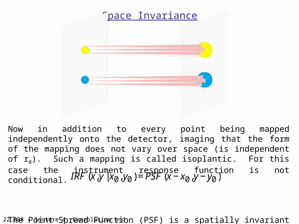
Now in addition to every point being mapped independently onto the detector, imaging that the form of the mapping does not vary over space (is independent of r0). Such a mapping is called isoplantic. For this case the instrument response function is not conditional.
The Point Spread Function (PSF) is a spatially invariant approximation of the IRF.
€
IRF(x,y|x0,y0)=PSF(x−x0,y−y0)
22.058 - lecture 4, Convolution and Fourier Convolution
Space Invariance
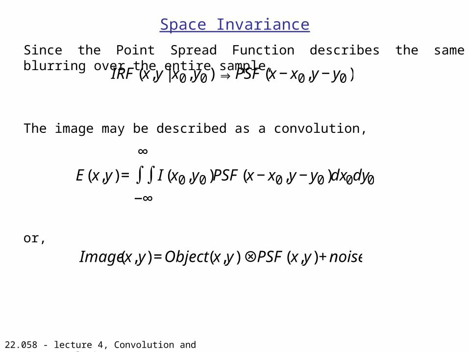
Since the Point Spread Function describes the same blurring over the entire sample,
The image may be described as a convolution,
or,
€
IRF(x,y|x0,y0)⇒ PSF(x−x0,y−y0)
€
E(x,y)=
∞
∫∫−∞
I (x0,y0)PSF(x−x0,y−y0)dx0dy0
€
Image(x,y)=Object(x,y)⊗PSF(x,y)+noise
22.058 - lecture 4, Convolution and Fourier Convolution
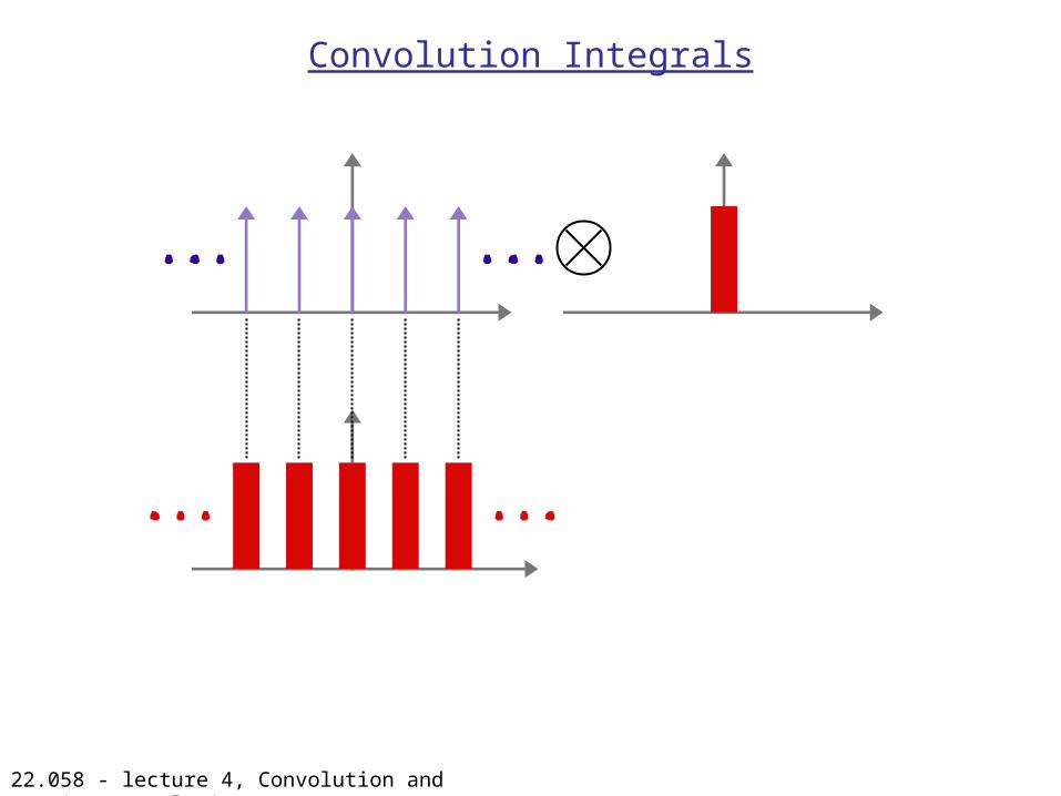
Convolution Integrals
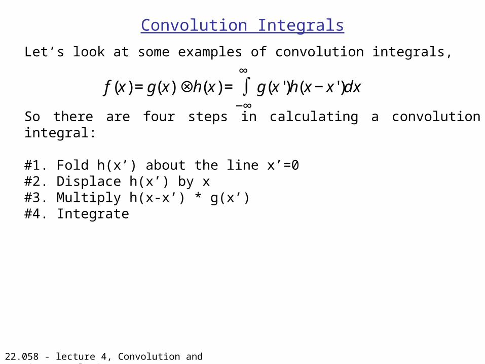
Let’s look at some examples of convolution integrals,
So there are four steps in calculating a convolution integral:
#1. Fold h(x’) about the line x’=0#2. Displace h(x’) by x#3. Multiply h(x-x’) * g(x’)#4. Integrate
€
f(x)=g(x)⊗h(x)=−∞
∞∫ g(x')h(x−x')dx'
22.058 - lecture 4, Convolution and Fourier Convolution
Convolution Integrals
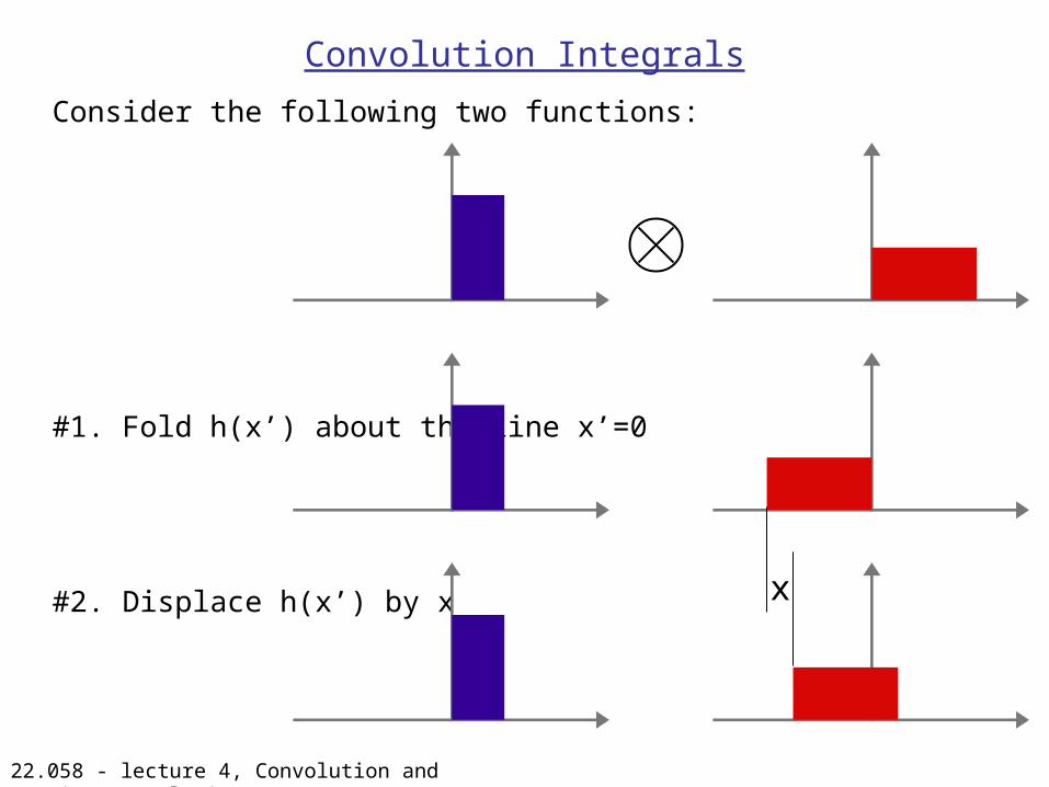
Consider the following two functions:
#1. Fold h(x’) about the line x’=0
#2. Displace h(x’) by x x
22.058 - lecture 4, Convolution and Fourier Convolution
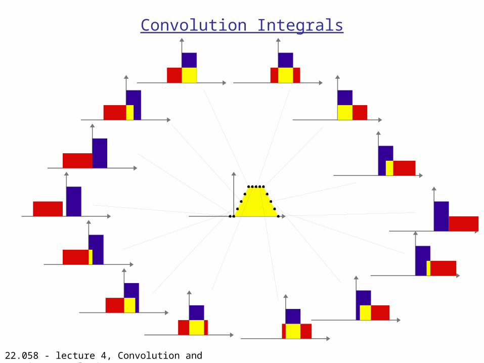
Convolution Integrals
22.058 - lecture 4, Convolution and Fourier Convolution
Convolution Integrals
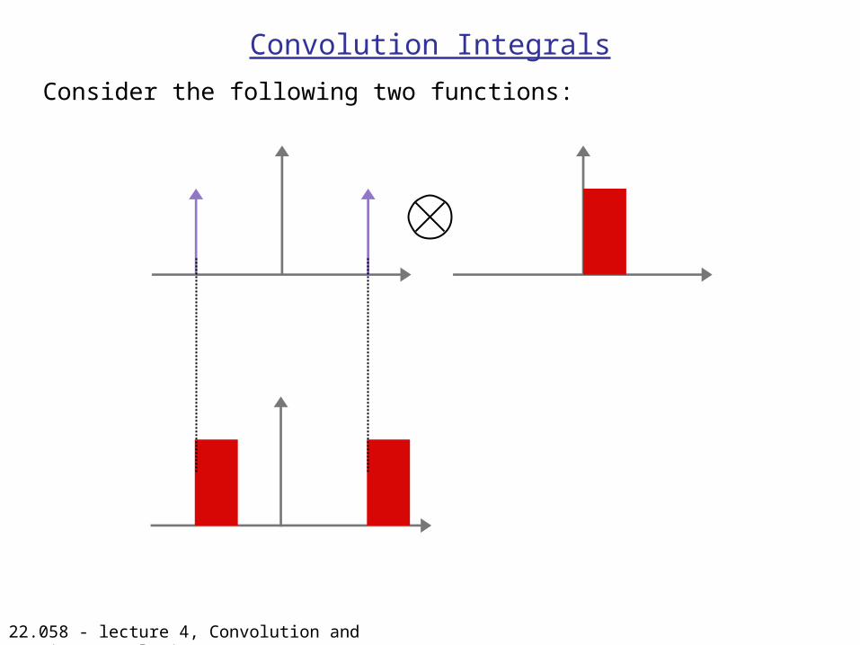
Consider the following two functions:
22.058 - lecture 4, Convolution and Fourier Convolution
Convolution Integrals
22.058 - lecture 4, Convolution and Fourier Convolution
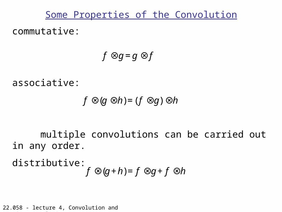
Some Properties of the Convolution
commutative:
associative:
multiple convolutions can be carried out in any order.
distributive:
€
f ⊗g=g⊗ f
€
f ⊗(g⊗h)=( f ⊗g)⊗h
€
f ⊗(g+h)=f ⊗g+f ⊗h
22.058 - lecture 4, Convolution and Fourier Convolution
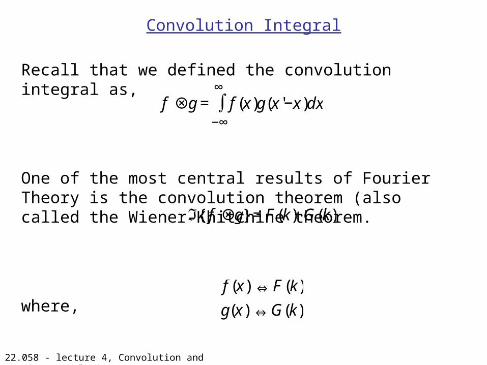
Recall that we defined the convolution integral as,
One of the most central results of Fourier Theory is the convolution theorem (also called the Wiener-Khitchine theorem.
where,
Convolution Integral
€
f ⊗g= f(x)g(x'−x)dx−∞
∞∫
€
ℑ f ⊗g{ }=F(k)⋅G(k)
€
f(x)⇔ F(k)
g(x)⇔ G(k)
22.058 - lecture 4, Convolution and Fourier Convolution
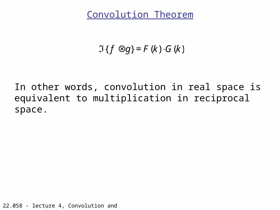
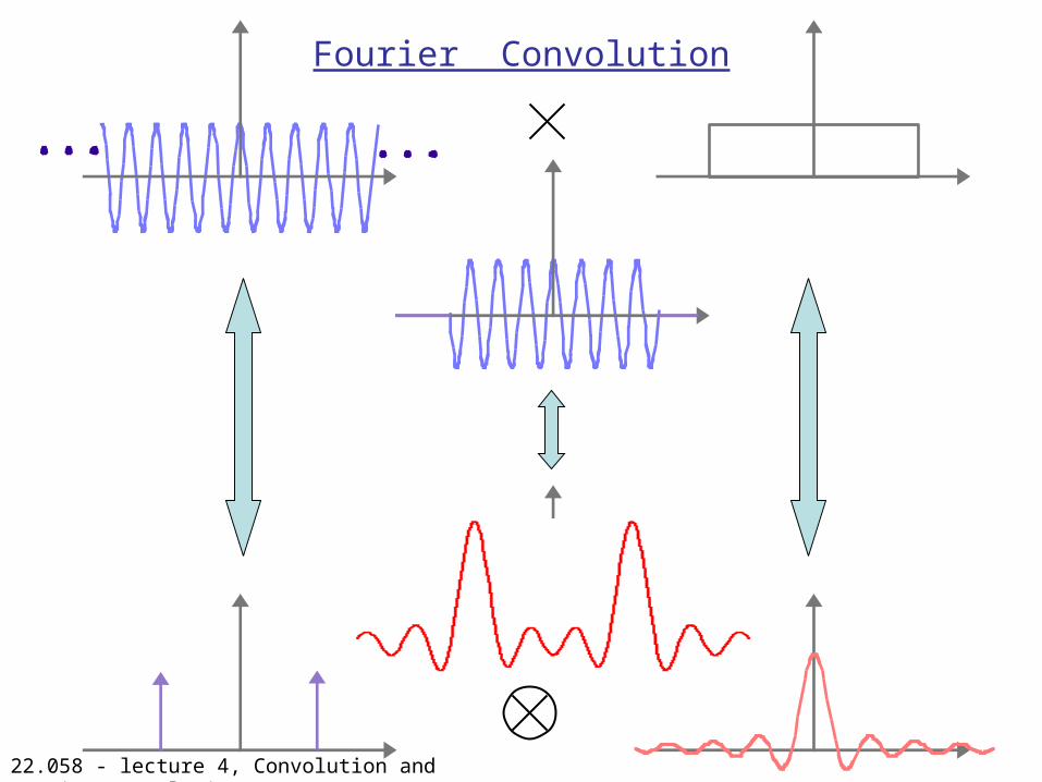
Convolution Theorem
In other words, convolution in real space is equivalent to multiplication in reciprocal space.
€
ℑ f ⊗g{ }=F(k)⋅G(k)
22.058 - lecture 4, Convolution and Fourier Convolution
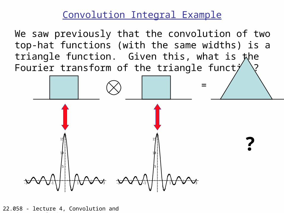
Convolution Integral Example
We saw previously that the convolution of two top-hat functions (with the same widths) is a triangle function. Given this, what is the Fourier transform of the triangle function?
-3 -2 -1 1 2 3
5
10
15
=
-3 -2 -1 1 2 3
5
10
15 ?
22.058 - lecture 4, Convolution and Fourier Convolution
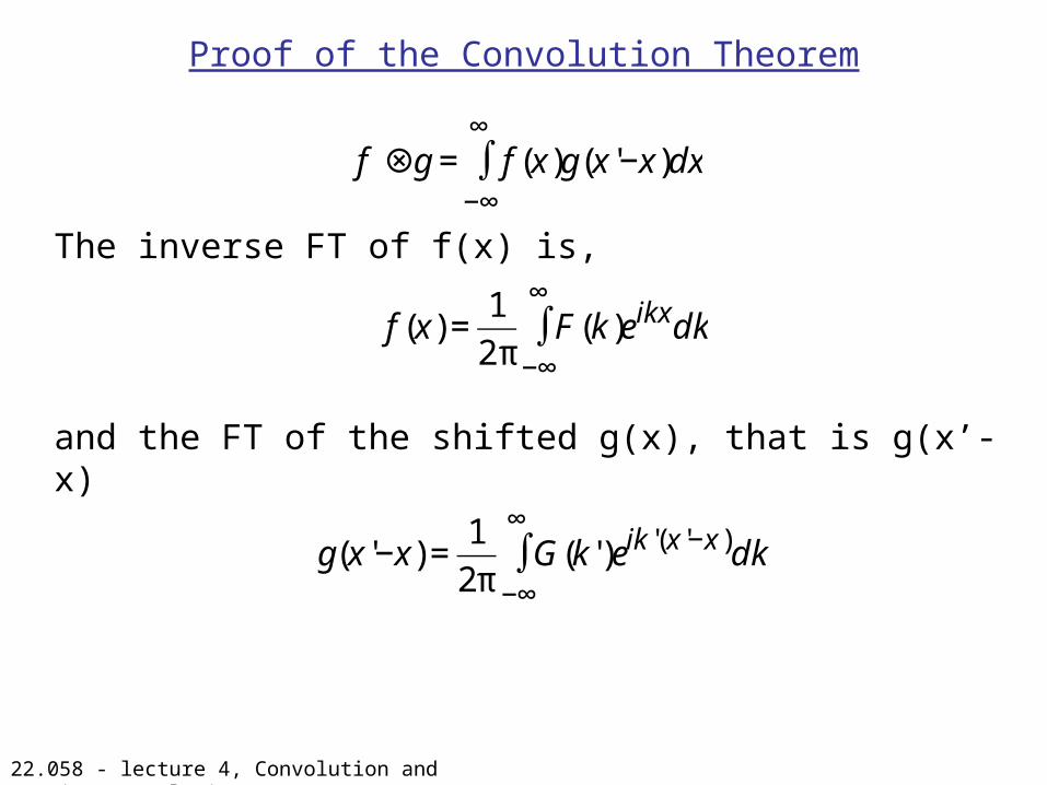
Proof of the Convolution Theorem
The inverse FT of f(x) is,
and the FT of the shifted g(x), that is g(x’-x)
€
f ⊗g= f(x)g(x'−x)dx−∞
∞∫
€
f(x)=12π
F(k)eikxdk−∞
∞∫
€
g(x'−x)=12π
G(k')eik'(x'−x)dk'−∞
∞∫
22.058 - lecture 4, Convolution and Fourier Convolution
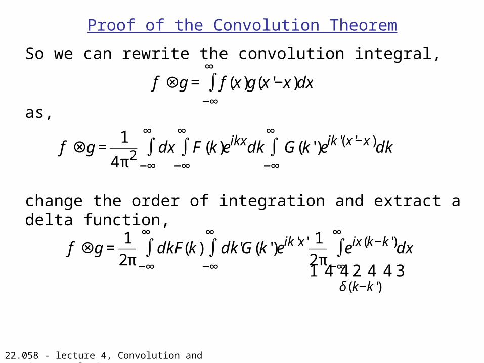
Proof of the Convolution Theorem
So we can rewrite the convolution integral,
as,
change the order of integration and extract a delta function,
€
f ⊗g= f(x)g(x'−x)dx−∞
∞∫
€
f ⊗g=1
4π2 dx F(k)eikxdk−∞
∞∫
−∞
∞∫ G(k')eik'(x'−x)dk'
−∞
∞∫
€
f ⊗g=12π
dkF(k) dk'G(k')eik'x'1
2πeix(k−k')dx
−∞
∞∫
δ(k−k')1 2 4 4 3 4 4 −∞
∞∫
−∞
∞∫
22.058 - lecture 4, Convolution and Fourier Convolution
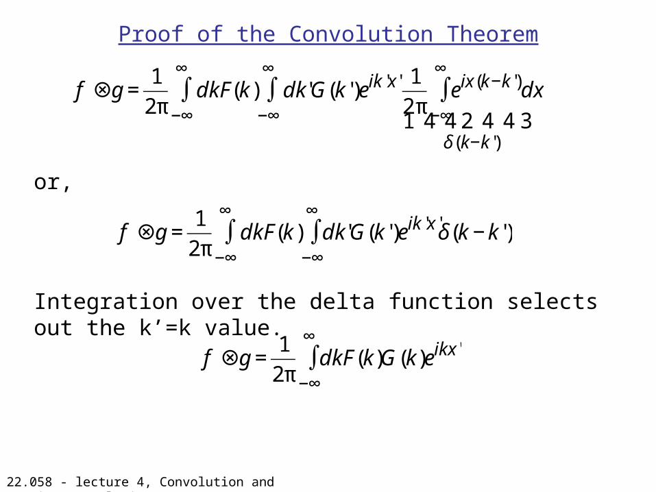
Proof of the Convolution Theorem
or,
Integration over the delta function selects out the k’=k value.
€
f ⊗g=12π
dkF(k) dk'G(k')eik'x'1
2πeix(k−k')dx
−∞
∞∫
δ(k−k')1 2 4 4 3 4 4 −∞
∞∫
−∞
∞∫
€
f ⊗g=12π
dkF(k) dk'G(k')eik'x'δ(k−k')−∞
∞∫
−∞
∞∫
€
f ⊗g=12π
dkF(k)G(k)eikx'
−∞
∞∫
22.058 - lecture 4, Convolution and Fourier Convolution
Proof of the Convolution Theorem
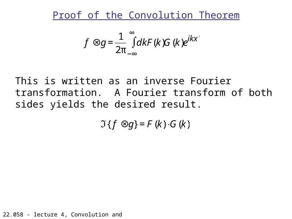
This is written as an inverse Fourier transformation. A Fourier transform of both sides yields the desired result.
€
f ⊗g=12π
dkF(k)G(k)eikx'
−∞
∞∫
€
ℑ f ⊗g{ }=F(k)⋅G(k)
22.058 - lecture 4, Convolution and Fourier Convolution
Fourier Convolution
22.058 - lecture 4, Convolution and Fourier Convolution
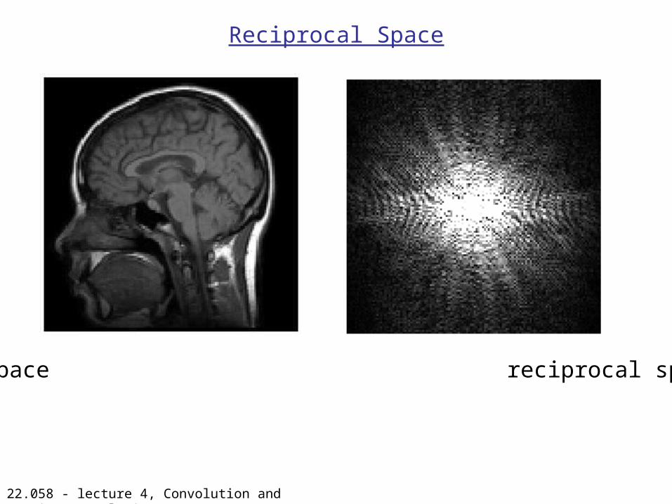
Reciprocal Space
real space reciprocal space
22.058 - lecture 4, Convolution and Fourier Convolution
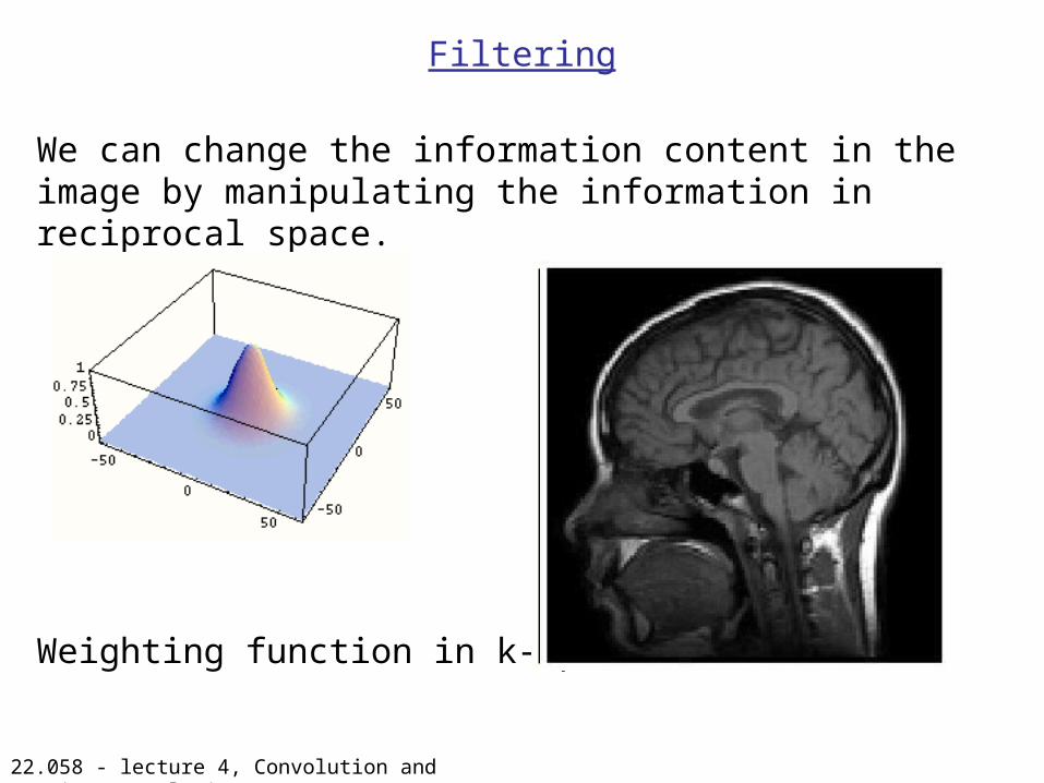
Filtering
We can change the information content in the image by manipulating the information in reciprocal space.
Weighting function in k-space.
22.058 - lecture 4, Convolution and Fourier Convolution
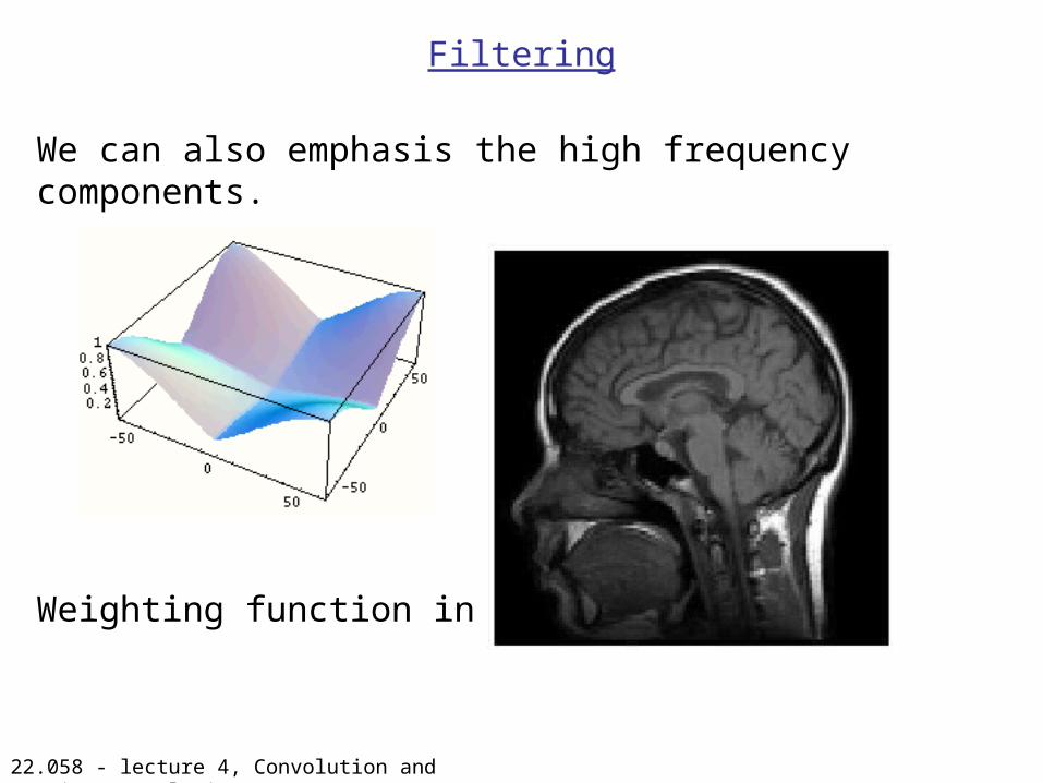
Filtering
We can also emphasis the high frequency components.
Weighting function in k-space.
22.058 - lecture 4, Convolution and Fourier Convolution
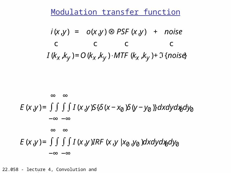
Modulation transfer function
€
i(x,y) = o(x,y)⊗ PSF(x,y) + noise
c c c c
I (kx,ky)=O(kx,ky)⋅MTF(kx,ky)+ℑ noise{ }
€
E(x,y)=
∞
∫∫−∞
∞
∫∫−∞
I (x,y)S δ(x−x0)δ(y−y0){ }dxdydx0dy0
E(x,y)=
∞
∫∫−∞
∞
∫∫−∞
I (x,y)IRF(x,y|x0,y0)dxdydx0dy0
22.058 - lecture 4, Convolution and Fourier Convolution
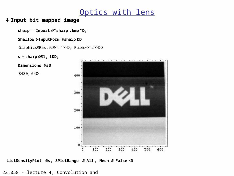
Optics with lens‡ Input bit mapped image
sharp =Import @"sharp. bmp"D;
Shallow @InputForm@sharpDD
Graphics@Raster@<< 4>>D, Rule@<< 2>>DD
s = sharp @@1, 1DD;
Dimensions @sD
8480, 640<
ListDensityPlot @s, 8PlotRange ÆAll , MeshÆFalse <D
22.058 - lecture 4, Convolution and Fourier Convolution
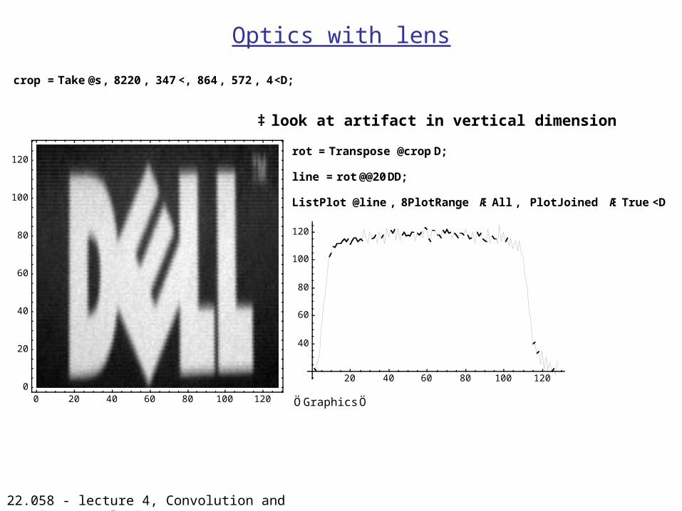
Optics with lens
crop =Take@s, 8220, 347<, 864, 572, 4<D;
‡ look at artifact in vertical dimension
rot =Transpose @crop D;
line =rot @@20DD;
ListPlot @line , 8PlotRange ÆAll , PlotJoined ÆTrue <D
20 40 60 80 100 120
40
60
80
100
120
Ö Graphics Ö0 20 40 60 80 100 1200
20
40
60
80
100
120
22.058 - lecture 4, Convolution and Fourier Convolution
Optics with lens
20 40 60 80 100 120
40
60
80
100
120
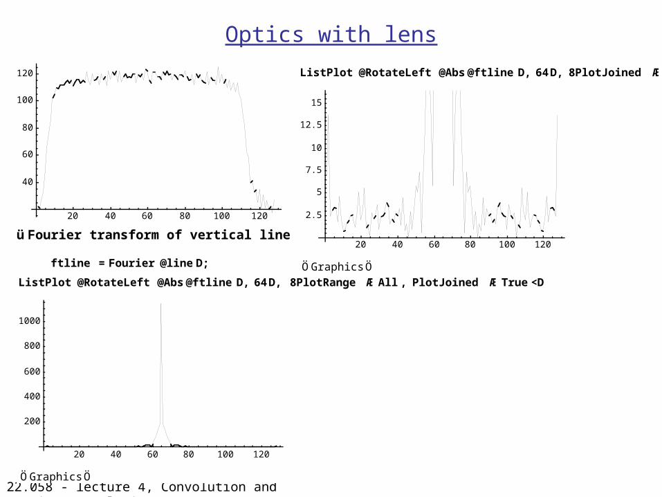
üFourier transform of vertical line to show modulation
ftline =Fourier @line D;
ListPlot @RotateLeft @Abs@ftline D, 64D, 8PlotJoined ÆTrue <D
20 40 60 80 100 120
2.5
5
7.5
10
12.5
15
Ö Graphics Ö
ListPlot @RotateLeft @Abs@ftline D, 64D, 8PlotRange ÆAll , PlotJoined ÆTrue <D
20 40 60 80 100 120
200
400
600
800
1000
Ö Graphics Ö
22.058 - lecture 4, Convolution and Fourier Convolution
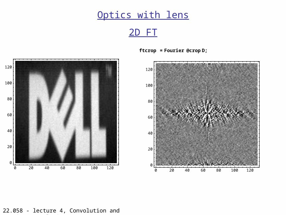
Optics with lens
2D FT
0 20 40 60 80 100 1200
20
40
60
80
100
120
ftcrop =Fourier @crop D;
0 20 40 60 80 100 1200
20
40
60
80
100
120
22.058 - lecture 4, Convolution and Fourier Convolution
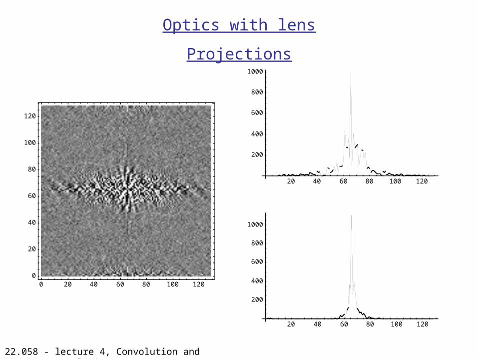
Optics with lens
Projections
0 20 40 60 80 100 1200
20
40
60
80
100
120
20 40 60 80 100 120
200
400
600
800
1000
20 40 60 80 100 120
200
400
600
800
1000
22.058 - lecture 4, Convolution and Fourier Convolution
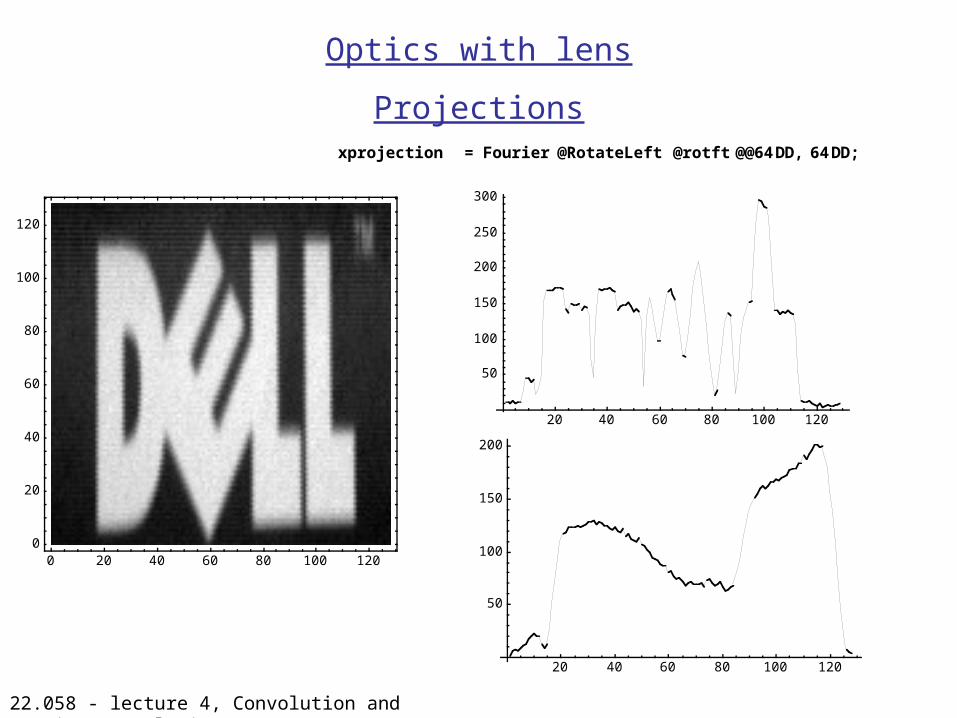
Optics with lens
Projections
0 20 40 60 80 100 1200
20
40
60
80
100
120
xprojection = Fourier @RotateLeft @rotft @@64DD, 64DD;
20 40 60 80 100 120
50
100
150
200
250
300
20 40 60 80 100 120
50
100
150
200
22.058 - lecture 4, Convolution and Fourier Convolution
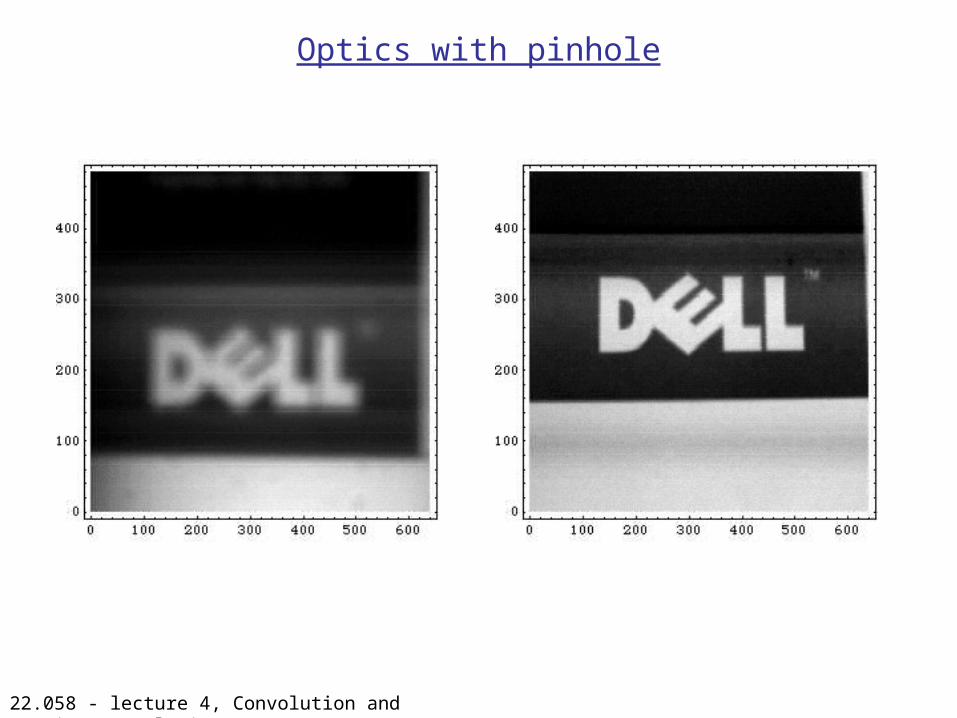
Optics with pinhole
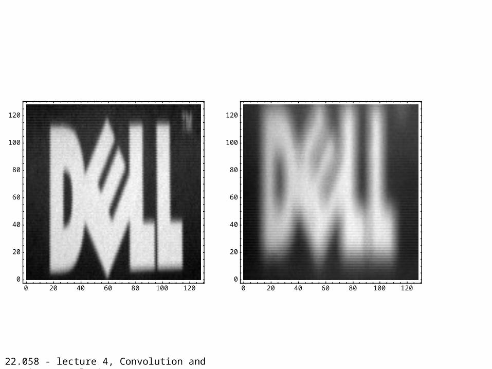
22.058 - lecture 4, Convolution and Fourier Convolution
0 20 40 60 80 100 1200
20
40
60
80
100
120
0 20 40 60 80 100 1200
20
40
60
80
100
120
22.058 - lecture 4, Convolution and Fourier Convolution
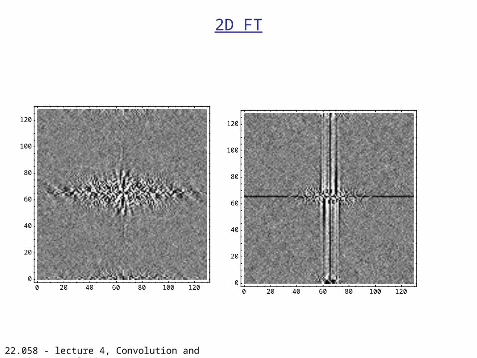
2D FT
0 20 40 60 80 100 1200
20
40
60
80
100
120
0 20 40 60 80 100 1200
20
40
60
80
100
120
22.058 - lecture 4, Convolution and Fourier Convolution
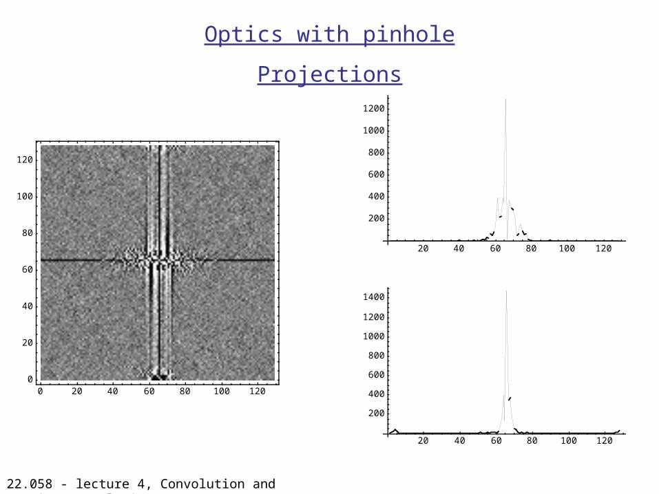
Optics with pinhole
Projections
0 20 40 60 80 100 1200
20
40
60
80
100
120
20 40 60 80 100 120
200
400
600
800
1000
1200
20 40 60 80 100 120
200
400
600
800
1000
1200
1400
22.058 - lecture 4, Convolution and Fourier Convolution
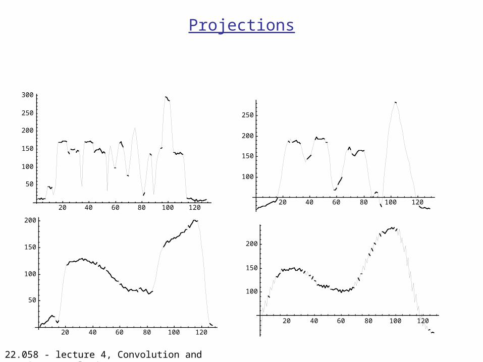
Projections
20 40 60 80 100 120
50
100
150
200
250
300
20 40 60 80 100 120
50
100
150
200
20 40 60 80 100 120
100
150
200
250
20 40 60 80 100 120
100
150
200
22.058 - lecture 4, Convolution and Fourier Convolution
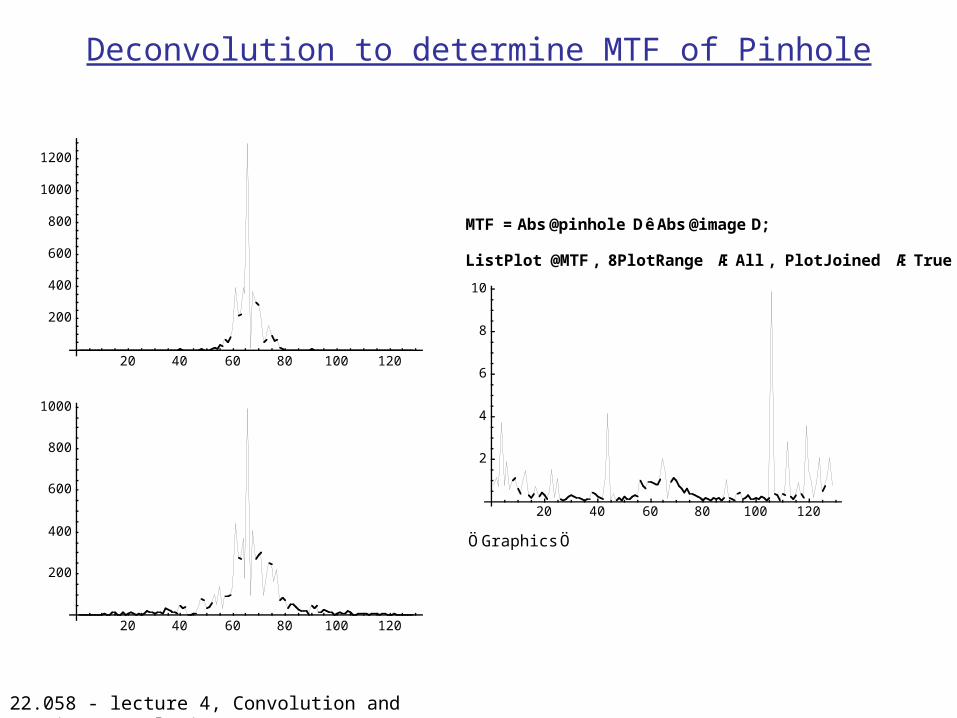
Deconvolution to determine MTF of Pinhole
20 40 60 80 100 120
200
400
600
800
1000
20 40 60 80 100 120
200
400
600
800
1000
1200
MTF=Abs@pinhole DêAbs@imageD;
ListPlot @MTF, 8PlotRange ÆAll , PlotJoined ÆTrue <D
20 40 60 80 100 120
2
4
6
8
10
Ö Graphics Ö
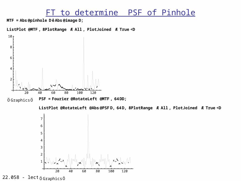
22.058 - lecture 4, Convolution and Fourier Convolution
FT to determine PSF of PinholeMTF=Abs@pinhole DêAbs@imageD;
ListPlot @MTF, 8PlotRange ÆAll , PlotJoined ÆTrue <D
20 40 60 80 100 120
2
4
6
8
10
Ö Graphics Ö PSF =Fourier @RotateLeft @MTF, 64DD;
ListPlot @RotateLeft @Abs@PSFD, 64D, 8PlotRange ÆAll , PlotJoined ÆTrue <D
20 40 60 80 100 120
1
2
3
4
5
6
7
Ö Graphics Ö
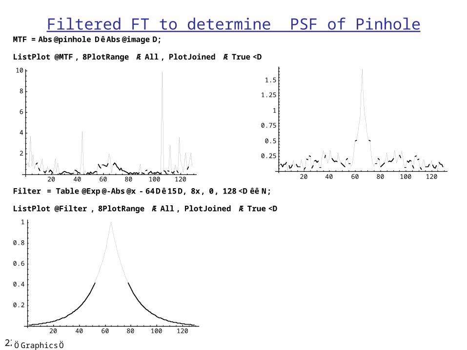
22.058 - lecture 4, Convolution and Fourier Convolution
Filtered FT to determine PSF of PinholeMTF=Abs@pinhole DêAbs@imageD;
ListPlot @MTF, 8PlotRange ÆAll , PlotJoined ÆTrue <D
20 40 60 80 100 120
2
4
6
8
10
Ö Graphics ÖFilter = Table @Exp@-Abs@x - 64Dê15D, 8x, 0, 128<DêêN;
ListPlot @Filter , 8PlotRange ÆAll , PlotJoined ÆTrue <D
20 40 60 80 100 120
0.2
0.4
0.6
0.8
1
Ö Graphics Ö
20 40 60 80 100 120
0.25
0.5
0.75
1
1.25
1.5