fourier transforms, generalised functions and … transforms, generalised functions and greens...

2015-01-23 Electromagnetic Processes In Dispersive Media, Lecture 2 - T. Johnson 1

Fourier transforms, Generalised functions and Greens functions

T. Johnson


Motivation

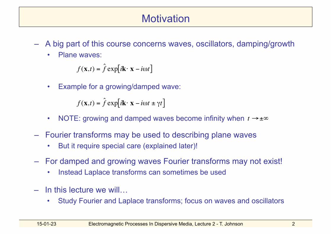
–  A big part of this course concerns waves, oscillators, damping/growth •  Plane waves:

•  Example for a growing/damped wave:

•  NOTE: growing and damped waves become infinity when

€

f (x,t) = ˆ f exp ik⋅ x − iωt[ ]

€

f (x,t) = ˆ f exp ik⋅ x − iωt ± γt[ ]

€

t →±∞

–  Fourier transforms may be used to describing plane waves •  But it require special care (explained later)!

–  In this lecture we will… •  Study Fourier and Laplace transforms; focus on waves and oscillators

–  For damped and growing waves Fourier transforms may not exist! •  Instead Laplace transforms can sometimes be used


Outline

–  Fourier transforms •  Fourier’s integral theorem •  Truncations and generalised functions •  Plemej formula

–  Laplace transforms and complex frequencies •  Theorem of residues •  Causal functions •  Relations between Laplace and Fourier transforms

–  Greens functions •  Poisson equation •  d’ Alemberts equation •  Wave equations in temporal gauge

–  Self-study: linear algebra and tensors


What functions can be Fourier transformed? •  The Fourier integral theorem:

–  f(t) is sectionally continuous over

–  f(t) is defined as

–  f(t) is amplitude integrable, that is,

Then the following identity holds:

€

f (t) =1f (t) = cos(t)

f (t) =0 , t < 0

exp(−t) , t ≥ 0⎧ ⎨ ⎩

f (t) =0 , t is a rational number

exp(−t 2) , t is an irrational number⎧ ⎨ ⎩

•  For which of the following functions does the above theorem hold?


What functions can be Fourier transformed?

Many commonly used functions are not amplitude integrable, e.g. f(t)=cos(t), f(t)=exp(it) and f(t)=1.

Solution: Use approximations of cos(t) that converge asymptotically to cos(t) – details comes later on

•  The asymptotic limits of functions like cos(t) will be used to define generalised functions, e.g. Dirac δ-function.


Dirac δ-function •  Dirac’s generalised function can be defined as:

Alternative definitions, as limits of well behaving functions, are shown shortly

•  Important example:

Proof: Whenever |f(t)|>0 the contribution is zero. For each t = ti where f(ti)=0, perform the integral over a small region ti – ε < t < ti + ε (where ε is small such f(t) ≈ (t - ti) f’(ti) ). Next, use variable substitution to perform the integration in x = f(t), then dt = dx / f’(ti) :

&

€

δ f (t)( )dt−∞

∞

∫ =i: f (ti )=0∑ 1

f '(ti)δ x( )dx =

−∞

∞

∫i: f (ti )=0∑ 1

f '(ti)

€

δ f (t)( )dt−∞

∞

∫ =i: f (ti )=0∑ 1

f '(ti)


Truncations and Generalised functions •  To approximate the Fourier transform of f(t)=1, use truncation.

•  Then for f(t)=1

–  When T→∞ then this function is zero everywhere except at ω=0 and its integral is 2π, i.e.

–  Note: F{1} exists only as an asymptotic of an ordinary function, i.e. a generalised function.

Truncation of a function f(t):

, such that

€

F fT (t){ } = fT (t)e− iωt

−∞

∞

∫ dt = 1e−iωt−T

T

∫ dt =sin(ωt /2)ω /2

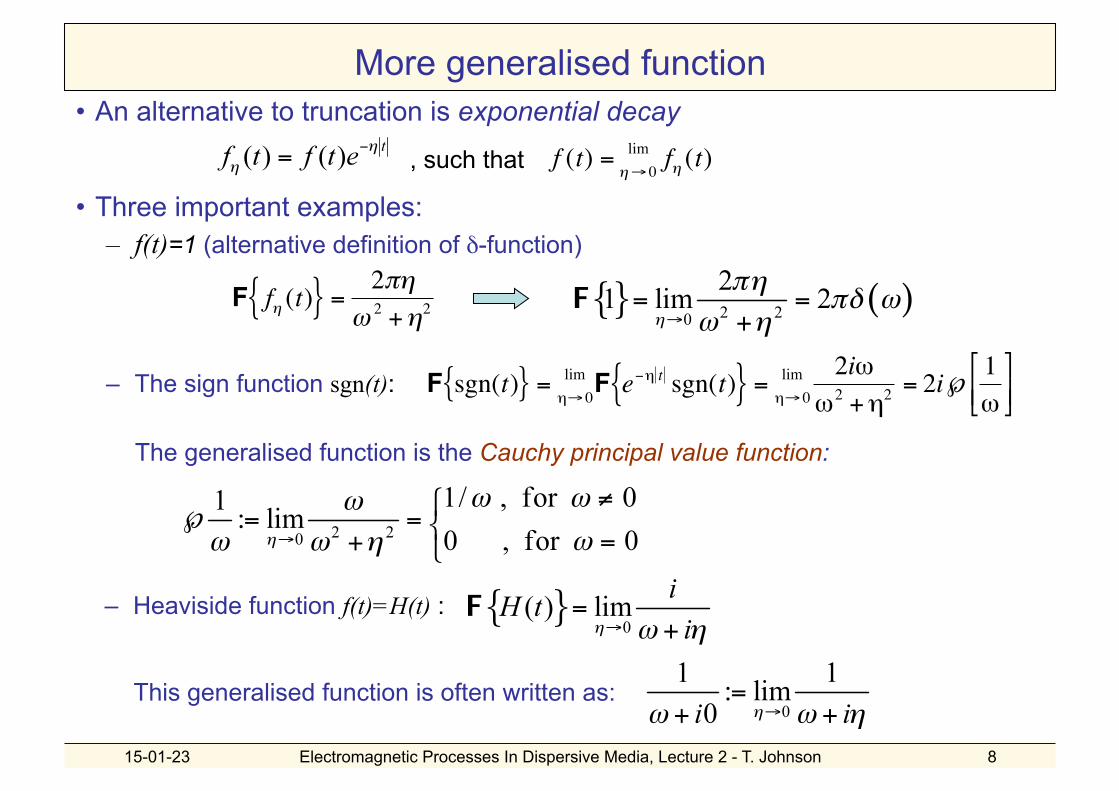
•  An alternative to truncation is exponential decay

–  The sign function sgn(t):

The generalised function is the Cauchy principal value function:

–  Heaviside function f(t)=H(t) :

This generalised function is often written as:


More generalised function

, such that

€

f (t) = limη→ 0

fη (t)

€

F fη (t){ } =2πη

ω 2 +η2

€

F sgn(t){ } = limη→ 0

F e−η t sgn(t){ } = limη→ 0

2iωω2 +η2

= 2i℘ 1ω

⎡

⎣ ⎢ ⎤

⎦ ⎥

•  Three important examples: –  f(t)=1 (alternative definition of δ-function)


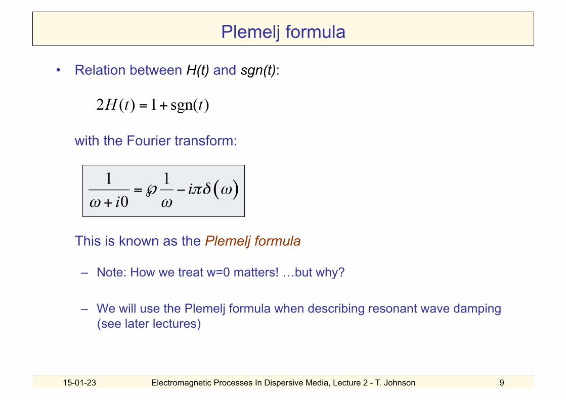
Plemelj formula

with the Fourier transform:

This is known as the Plemelj formula

•  Relation between H(t) and sgn(t):

–  Note: How we treat w=0 matters! …but why?

–  We will use the Plemelj formula when describing resonant wave damping (see later lectures)

•  Fourier transform:

•  Solution:

where •  Take limit when damping ν goes to zero:

use Plemelj formula


Driven oscillator with dissipation •  Example of the Plemelj formula: a driven oscillator with

eigenfrequency Ω :

with dissipation coefficient ν :

Later we’ll look at the inverse transform


Physics interpretation of Plemej formula •  For oscillating systems:

eigenfrequency Ω will appear as resonant denominator

Including infinitely small dissipation and applying Plemelj formula

•  Later lectures on the dielectric response of plasma: When the dissipation goes to zero for a kinetic plasma there is still a wave damping called Landau damping, a “collisionless” damping, which comes from the δ-function

€

f (ω) ~ 1ω ±Ω

⇔ f (t) ~ e±iΩt


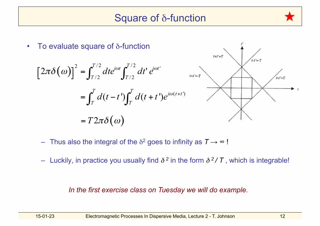
Square of δ-function

•  To evaluate square of δ-function

–  Thus also the integral of the δ2 goes to infinity as T → ∞ !

–  Luckily, in practice you usually find δ 2 in the form δ 2 / T , which is integrable!

In the first exercise class on Tuesday we will do example.


Outline






Laplace transforms and complex frequencies (Chapter 8)

•  Fourier transform is restricted to handling real frequencies, i.e. not optimal for damped or growing modes

–  For this purpose we need the Laplace transforms, which allow us to study complex frequencies.

•  To understand better the relation between Fourier and Laplace transforms we will first study the residual theorem and see it applied to the Fourier transform of causal functions.


The Theorem of Residues

•  Expand f(z) around singularity, z=zi:

–  the point z=zi is called a pole –  the numerator Ri is the residue €

f (z) ≈ Ri

(z − zi)+ c0 + c1(z − zi) + ...

€

f (z)dz =C∫ 2πi Ri

i∑

•  The integral along closed contour in the complex plane can be solved using the theorem of residues

–  where the sum is over all poles zi inside the contour

Im(ω)

Re(ω)

C

Poles zi


Example: Theorem of Residues

•  Example: f(z)=1/z and C encircling a poles at z=0


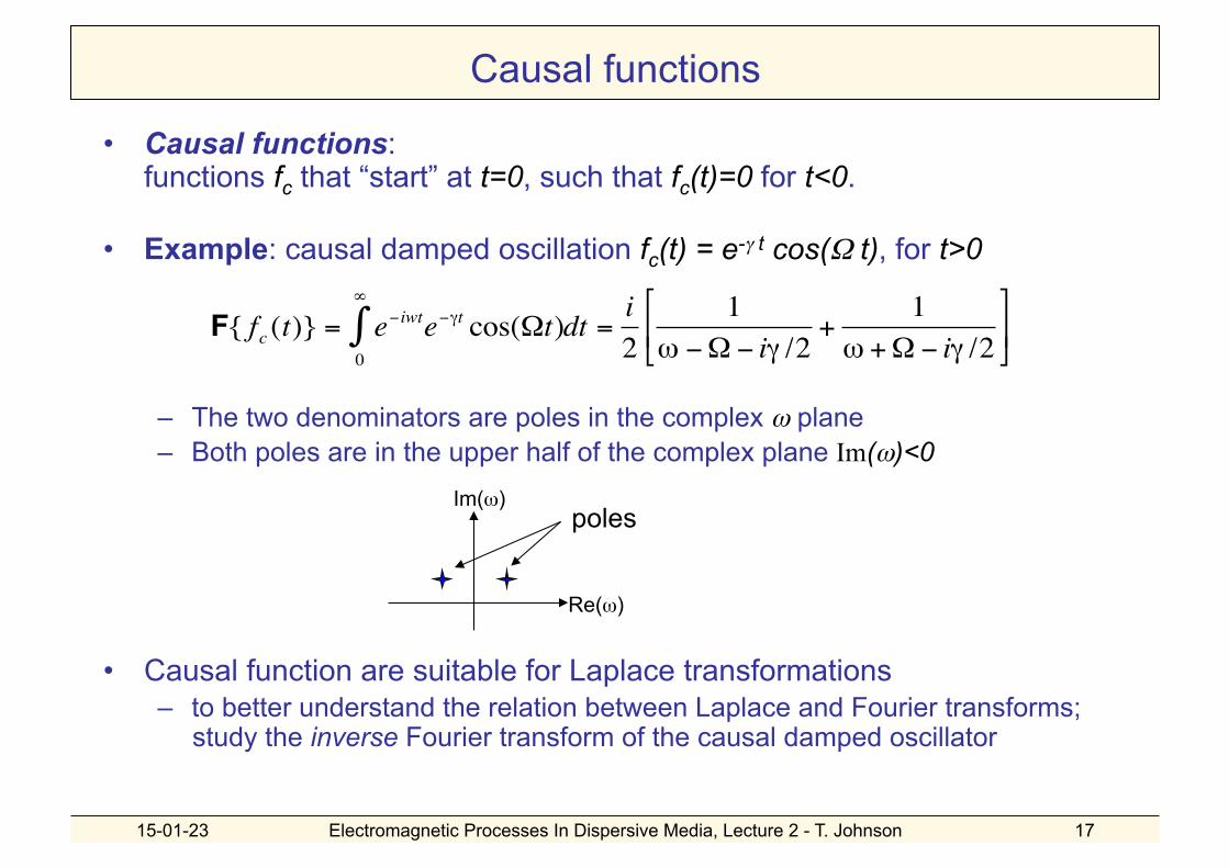
Causal functions

•  Causal functions: functions fc that “start” at t=0, such that fc(t)=0 for t<0.

•  Example: causal damped oscillation fc(t) = e-γ t cos(Ω t), for t>0

–  The two denominators are poles in the complex ω plane –  Both poles are in the upper half of the complex plane Im(ω)<0

•  Causal function are suitable for Laplace transformations –  to better understand the relation between Laplace and Fourier transforms;

study the inverse Fourier transform of the causal damped oscillator

poles Im(ω)

Re(ω)

€

F{ fc (t)} = e−iwte−γt cos(Ωt)0

∞

∫ dt =i2

1ω −Ω − iγ /2

+1

ω +Ω− iγ /2⎡

⎣ ⎢

⎤

⎦ ⎥


Causal functions and contour integration

•  Use Residual analysis for inverse Fourier transform of the causal damped oscillation

€

fc (t) =12π

eiωtC∫ i

21

ω −Ω+ iγ /2+

1ω +Ω+ iγ /2

⎡

⎣ ⎢

⎤

⎦ ⎥ dω

= − iRii∑ = −i i

2e(iΩ−γ / 2)t + e(− iΩ−γ / 2)t[ ]

€

F−1{ fc (t)} =1

2πdω eiωt∫ i

21

ω −Ω − iγ /2+

1ω +Ω− iγ /2

⎡

⎣ ⎢

⎤

⎦ ⎥

⎧ ⎨ ⎩

⎫ ⎬ ⎭

t<0 Im(ω)

Re(ω)

C

t>0 Im(ω)

Re(ω)

C

For t > 0: –  For Im(ω) →∞ , then eiωt →0 and

–  Thus, close contour with half circle Im(ω)>0

–  Inverse Fourier transform is sum of residues from poles

For t < 0: –  eiωt →0 , for Im(ω) →-∞;

close contour with half circle Im(ω)<0 –  No poles inside contour: f(t)=0 for t<0

€

limω →∞

˜ f c (ω ) ~ 1/ω →0


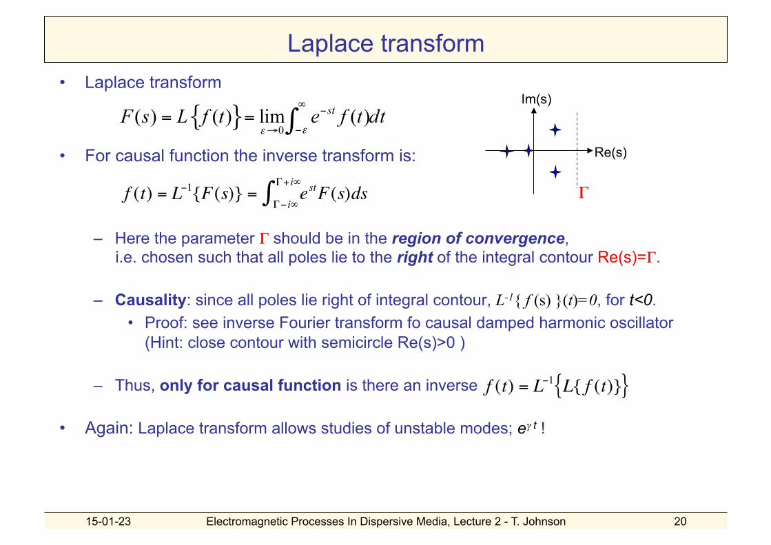
Laplace transform •  Laplace transform of function f(t) is

–  Like a Fourier transform for a causal function, but iω → s.

•  Region of convergence: –  Note: For Re(s)<0 the integral may not converge since the factor e-st diverges

–  Consider function

F(s) is integrable only if

Thus, the Laplace transform is only valid for

Note: means pole at s=ν, i.e. poles must be to the right of the region of convergence

–  Laplace transform allows studies of unstable modes; eγ t !

Im(s)

Re(s)

L{ f(t) } converges! €

f (t) = eνt ⇒ F(s) = e(ν−s)t0

∞

∫ dt


Laplace transform •  Laplace transform

•  For causal function the inverse transform is:

–  Here the parameter Γ should be in the region of convergence, i.e. chosen such that all poles lie to the right of the integral contour Re(s)=Γ.

–  Causality: since all poles lie right of integral contour, L-1{ f (s) }(t)=0, for t<0. •  Proof: see inverse Fourier transform fo causal damped harmonic oscillator

(Hint: close contour with semicircle Re(s)>0 )

–  Thus, only for causal function is there an inverse

•  Again: Laplace transform allows studies of unstable modes; eγ t !

Γ

Im(s)

Re(s)

€

€

f (t) = L−1{F(s)} = estF(s)dsΓ− i∞

Γ+ i∞∫

€

f (t) = L−1 L{ f (t)}{ }


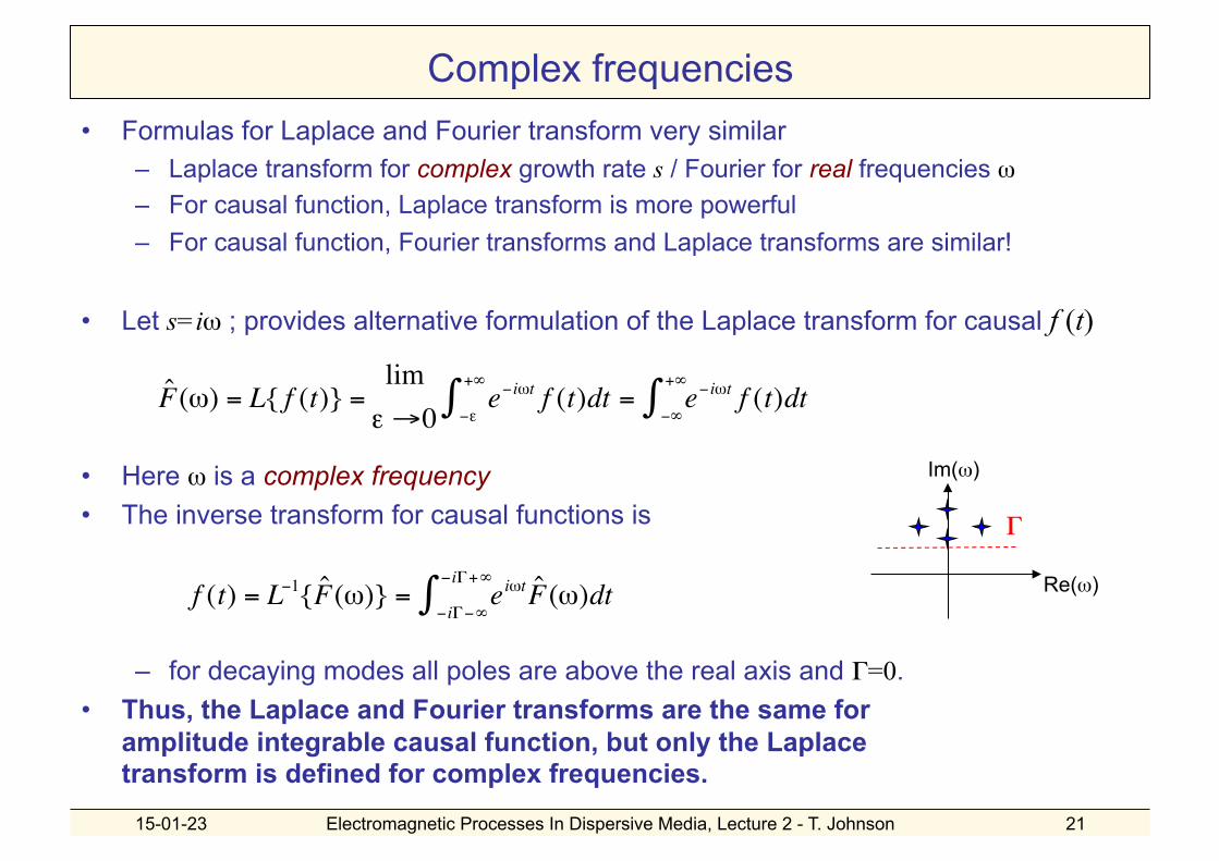
Complex frequencies •  Formulas for Laplace and Fourier transform very similar

–  Laplace transform for complex growth rate s / Fourier for real frequencies ω –  For causal function, Laplace transform is more powerful –  For causal function, Fourier transforms and Laplace transforms are similar!

•  Let s=iω ; provides alternative formulation of the Laplace transform for causal f (t)

•  Here ω is a complex frequency •  The inverse transform for causal functions is

–  for decaying modes all poles are above the real axis and Γ=0. •  Thus, the Laplace and Fourier transforms are the same for

amplitude integrable causal function, but only the Laplace transform is defined for complex frequencies.

Γ

Im(ω)

Re(ω)

€

€

ˆ F (ω) = L{ f (t)} =limε →0

e−iωt f (t)dt−ε

+∞

∫ = e− iωt f (t)dt−∞

+∞

∫

€

f (t) = L−1{ ˆ F (ω)} = eiωt ˆ F (ω)dt−iΓ−∞

−iΓ+∞

∫


Outline






Greens functions (Chapter 5) •  Greens functions: technique to solve inhomogeneous equations •  Linear differential equation for f given source S:

–  Where the differential operator L is of the form:

•  Ansatz: given the Greens function, then there is a solution:

•  Proof:

€

L(z) f (z) = L(z)∫ G(z,z')S(z')dz'= δ(z − z')∫ S(z')dz'= S(z)€

f (z) = G(z,z')S(z')dz'∫

•  Define Greens function G to solve:

–  the response from a point source – e.g. the fields from a particle!


How to calculate Greens functions? •  For differential equations without

explicit dependence on z, then

–  we may rewrite G as:

•  Fourier transform from z-z’ to k :

•  Inverse Fourier transform

Solve integral!

€

L(z − z')G(z − z') = δ(z − z')€

G(z,z')→G(z − z')

€

G(z − z') =12π

G(k)e−ik(z−z' )−∞

∞

∫ dk =12π

1L(ik)

e−ik(z−z' )−∞

∞

∫ dk

Example:

€

−ω2 +Ω2( )G(ω) = 2π

€

G(ω) = −2π

ω2 −Ω2

€

∂2

∂t 2+Ω2

⎛

⎝ ⎜

⎞

⎠ ⎟ G(t − t ') = δ(t − t')

€

L(z) = L(z − z')


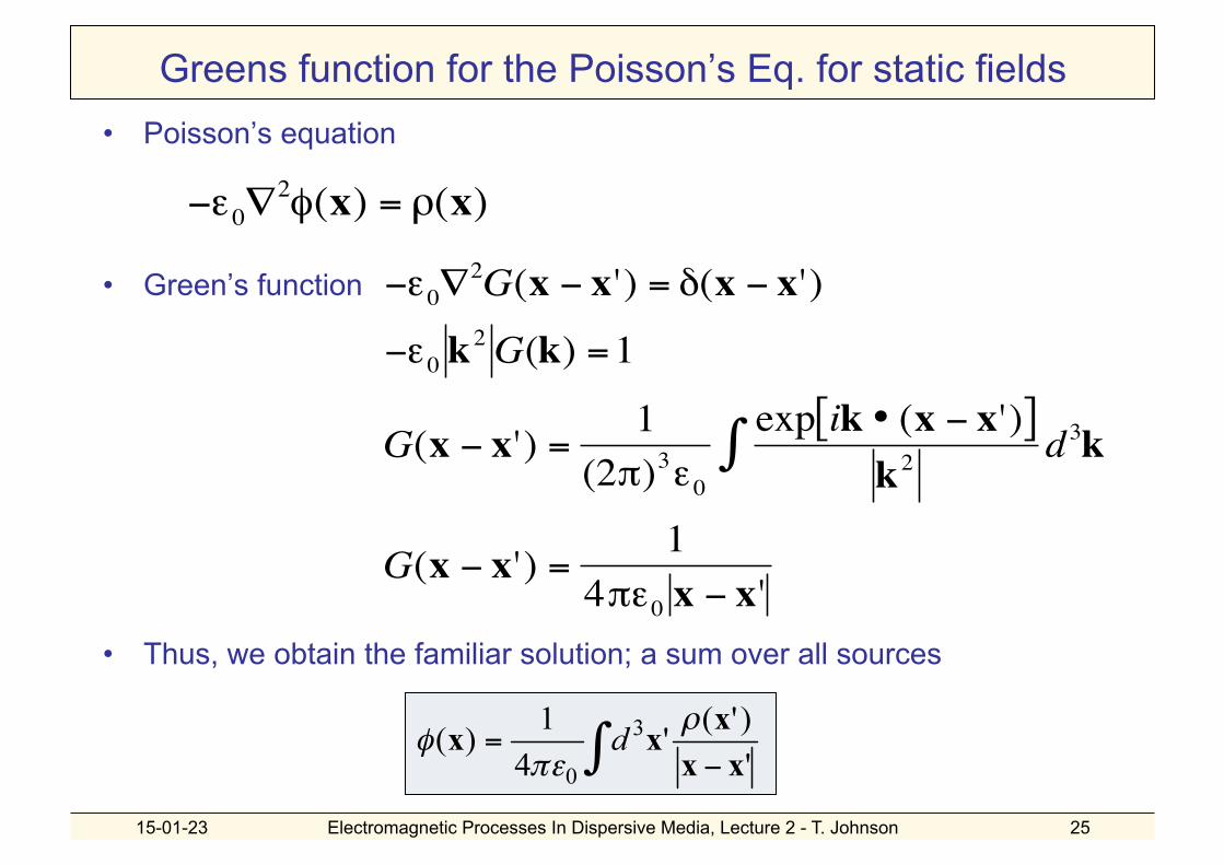
Greens function for the Poisson’s Eq. for static fields •  Poisson’s equation

•  Green’s function

•  Thus, we obtain the familiar solution; a sum over all sources

€

−ε0∇2φ(x) = ρ(x)

€

−ε0∇2G(x − x') = δ(x − x')

−ε0 k2G(k) =1

G(x − x') =1

(2π)3ε0exp ik • (x − x')[ ]

k2d3k∫

G(x − x') =1

4πε0 x − x'


Greens Function for d’Alembert’s Eq. (time dependent field)

•  D’Alembert’s Eq. has a Green function G(t,x)

•  Fourier transform gives

–  Information is propagating radially away from the source at the speed of light

€

1c 2

∂2

∂t 2−∇2

⎛

⎝ ⎜

⎞

⎠ ⎟ G(t − t ',x − x') = µ0δ(t − t ')δ

3(x − x')

€

G(t − t',x − x') =µ0

4π x − x'δ(t − t '−x − x' /c)

€

(t − t ',x − x')→(ω,k)


Greens Function for the Temporal Gauge •  Temporal gauge gives different form of wave equation

–  Different response in longitudinal :

–  and transverse directions:

•  To separate the longitudinal and transverse parts the Greens function become a 2-tensor Gij

•  Solution has poles ω = ± |k| c :


Outline






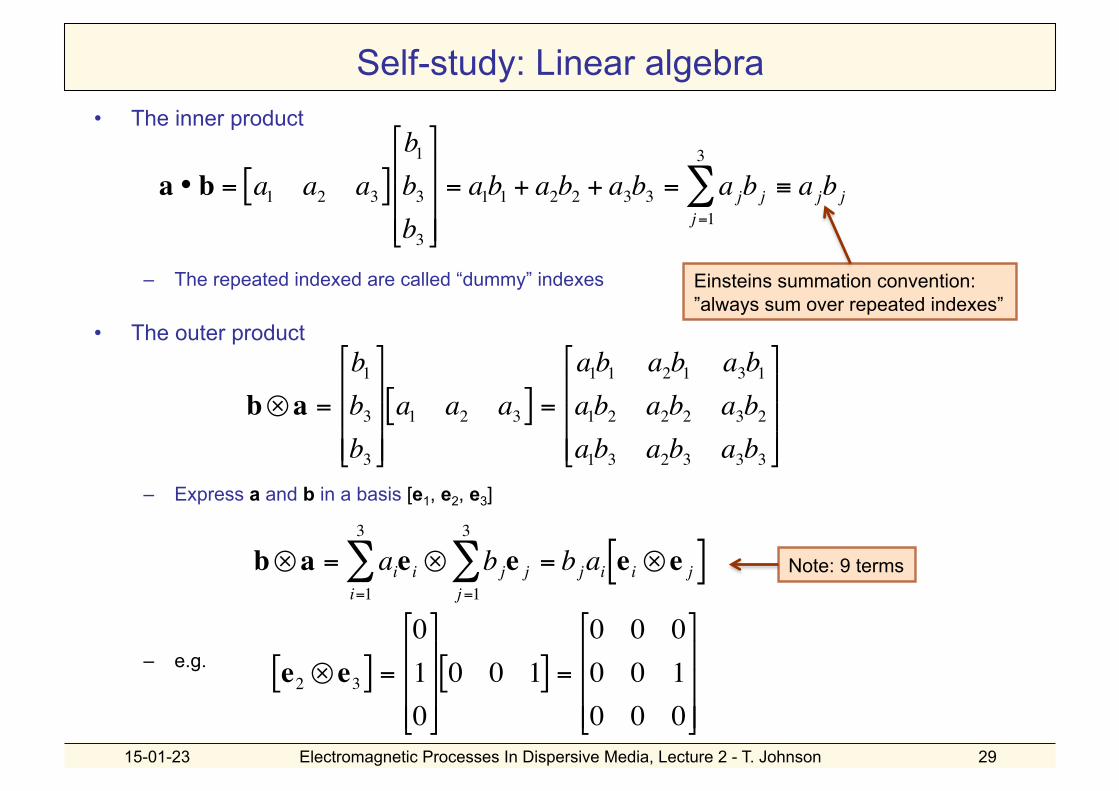
Self-study: Linear algebra •  The inner product

–  The repeated indexed are called “dummy” indexes

•  The outer product

–  Express a and b in a basis [e1, e2, e3]

–  e.g.

€

a • b = a1 a2 a3[ ]b1b3b3

⎡

⎣

⎢ ⎢ ⎢

⎤

⎦

⎥ ⎥ ⎥

= a1b1 + a2b2 + a3b3 = a jb jj=1

3

∑ ≡ a jb j

Einsteins summation convention: ”always sum over repeated indexes”

€

b⊗a =

b1b3b3

⎡

⎣

⎢ ⎢ ⎢

⎤

⎦

⎥ ⎥ ⎥ a1 a2 a3[ ] =

a1b1 a2b1 a3b1a1b2 a2b2 a3b2a1b3 a2b3 a3b3

⎡

⎣

⎢ ⎢ ⎢

⎤

⎦

⎥ ⎥ ⎥

€

b⊗a = aie ii=1

3

∑ ⊗ bje jj=1

3

∑ = b jai e i ⊗ e j[ ]

€

e2 ⊗ e3[ ] =

010

⎡

⎣

⎢ ⎢ ⎢

⎤

⎦

⎥ ⎥ ⎥ 0 0 1[ ] =

0 0 00 0 10 0 0

⎡

⎣

⎢ ⎢ ⎢

⎤

⎦

⎥ ⎥ ⎥

Note: 9 terms


Self-study: Vectors •  Vectors are defined by a length and a direction.

–  Note that the direction is independent of the coordinate system, thus the components depend on the coordinate system

–  thus in the (x, y) systems the components may be:

–  then for 30 degrees between the coordinate systems (u, v) components are:

•  The relation between vectors are given by transformation matrixes –  if transformation is a rotation then transformation matrixes

€

F = Fie i = Fi 'e i 'e1

e2

e1’

e2’

F

€

F1F2

⎡

⎣ ⎢

⎤

⎦ ⎥ =

11⎡

⎣ ⎢ ⎤

⎦ ⎥

€

F1'F2 '⎡

⎣ ⎢

⎤

⎦ ⎥ =

1/23/2

⎡

⎣ ⎢

⎤

⎦ ⎥

€

Fi '= RijFj ; Rij[ ] ≡ R11 R12

R21 R22

⎡

⎣ ⎢

⎤

⎦ ⎥ =

cos(ν) −sin(ν)sin(ν) cos(ν)⎡

⎣ ⎢

⎤

⎦ ⎥


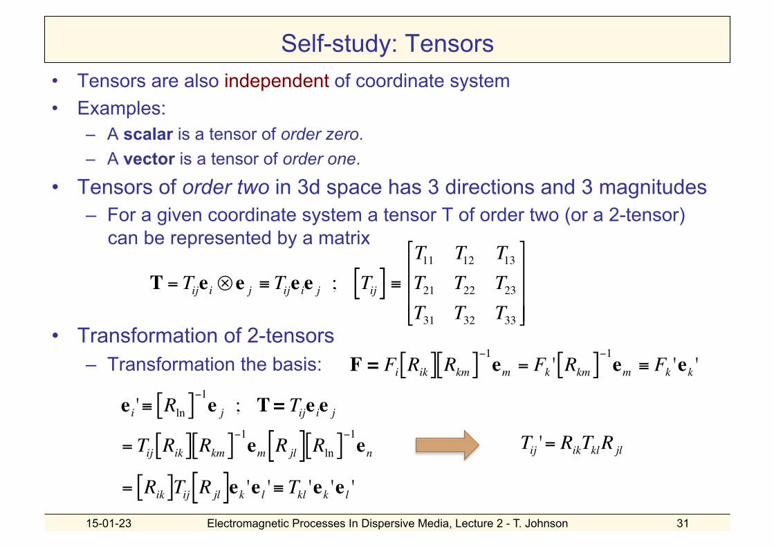
Self-study: Tensors •  Tensors are also independent of coordinate system •  Examples:

–  A scalar is a tensor of order zero. –  A vector is a tensor of order one.

•  Tensors of order two in 3d space has 3 directions and 3 magnitudes –  For a given coordinate system a tensor T of order two (or a 2-tensor)

can be represented by a matrix

•  Transformation of 2-tensors –  Transformation the basis:

€

T = Tije i ⊗ e j ≡ Tije ie j ; Tij[ ] ≡T11 T12 T13

T21 T22 T23

T31 T32 T33

⎡

⎣

⎢ ⎢ ⎢

⎤

⎦

⎥ ⎥ ⎥

€

e i '≡ Rln[ ]−1e j ; T= Tije ie j

= Tij Rik[ ] Rkm[ ]−1em R jl[ ] Rln[ ]−1

en

= Rik[ ]Tij R jl[ ]ek 'e l '≡ Tkl 'ek 'e l '€

Tij '= RikTklR jl€

F = Fi Rik[ ] Rkm[ ]−1em = Fk ' Rkm[ ]−1em ≡ Fk 'ek '

fourier transforms, generalised functions and … transforms, generalised functions and greens...

Documents