CERTAIN MULTIPLEGENERATING FUNCTIONS

AND INTEGRAL TRANSFORMSOF SPECIAL FUNCTIONS

TALHA USMAN

August 2, 2016

CERTAIN MULTIPLEGENERATING FUNCTIONS

AND INTEGRAL TRANSFORMSOF SPECIAL FUNCTIONS

THESIS

SUBMITTED FOR THE AWARD OF THE DEGREE OF

DOCTOR OF PHILOSOPHY

IN

APPLIED MATHEMATICS

BY

TALHA USMAN

UNDER THE SUPERVISION OF

DR. NABIULLAH KHAN

DEPARTMENT OF APPLIED MATHEMATICSFACULTY OF ENGINEERING & TECHNOLOGY

ALIGARH MUSLIM UNIVERSITY

ALIGARH-202002, INDIA

2016

Table of Contents

Acknowledgement vi

Preface viii

1 Preliminaries 1

1.1 Introduction . . . . . . . . . . . . . . . . . . . . . . . . . . . . . . . . 1

1.2 Gaussian Hypergeometric Functions and Its Applications . . . . . . . 3

1.3 Hypergeometric Functions of Two Variables . . . . . . . . . . . . . . 10

1.4 Hypergeometric Functions of Several Variables . . . . . . . . . . . . . 13

1.5 Bessel Functions . . . . . . . . . . . . . . . . . . . . . . . . . . . . . 16

1.6 Mittag-Leffler Functions . . . . . . . . . . . . . . . . . . . . . . . . . 18

1.7 Whittaker Functions . . . . . . . . . . . . . . . . . . . . . . . . . . . 21

1.8 The Classical Orthogonal Polynomials . . . . . . . . . . . . . . . . . 23

1.9 Generating Functions . . . . . . . . . . . . . . . . . . . . . . . . . . . 30

1.10 Integral Transforms . . . . . . . . . . . . . . . . . . . . . . . . . . . . 33

2 On Certain Mixed Generating Functions Involving the Product of

Jacobi Polynomials 36

2.1 Introduction . . . . . . . . . . . . . . . . . . . . . . . . . . . . . . . . 36

2.2 Generating Relation for the Product of Jacobi Polynomials . . . . . . 40

2.3 Special Cases . . . . . . . . . . . . . . . . . . . . . . . . . . . . . . . 41

i

3 Some New Class of Laguerre-Based Generalized Apostol type Poly-

nomials 45

3.1 Introduction . . . . . . . . . . . . . . . . . . . . . . . . . . . . . . . . 45

3.2 Definition and Properties of the Generalized Apostol type Laguerre-

Based Polynomials-I . . . . . . . . . . . . . . . . . . . . . . . . . . . 51

3.3 Implicit Summation Formulae Involving Apostol type Laguerre-Based

Polynomials-I . . . . . . . . . . . . . . . . . . . . . . . . . . . . . . . 53

3.4 General Symmetry Identities for the Generalized Apostol type Laguerre-

Based Polynomials-I . . . . . . . . . . . . . . . . . . . . . . . . . . . 63

3.5 Definition and Properties of the Generalized Apostol type Laguerre-

Based Polynomials-II . . . . . . . . . . . . . . . . . . . . . . . . . . . 68

3.6 Implicit Summation Formulae Involving Apostol type Laguerre-Based

Polynomials-II . . . . . . . . . . . . . . . . . . . . . . . . . . . . . . . 71

3.7 General Symmetry Identities for the Generalized Apostol type Laguerre-

Based Polynomials-II . . . . . . . . . . . . . . . . . . . . . . . . . . . 79

4 A new class of Laguerre poly-Bernoulli, poly-Euler and poly-Genocchi

Polynomials 85

4.1 Introduction . . . . . . . . . . . . . . . . . . . . . . . . . . . . . . . . 85

4.2 A new class of Laguerre poly-Bernoulli numbers and polynomials . . 91

4.3 Implicit summation formulae involving Laguerre poly-Bernoulli poly-

nomials . . . . . . . . . . . . . . . . . . . . . . . . . . . . . . . . . . 94

4.4 General symmetry identities for Laguerre poly-Bernoulli polynomials 99

4.5 Definition and Properties of the Laguerre poly-Euler polynomials and

Laguerre multi poly-Euler polynomials . . . . . . . . . . . . . . . . . 102

4.6 Implicit Summation Formulae Involving Laguerre poly-Euler Polyno-

mials . . . . . . . . . . . . . . . . . . . . . . . . . . . . . . . . . . . . 105

4.7 General Symmetry Identities for Laguerre poly-Euler Polynomials . . 111

4.8 A new class of Laguerre poly-Genocchi polynomials . . . . . . . . . . 114

4.9 Implicit summation formulae involving Laguerre poly-Genocchi poly-

nomials . . . . . . . . . . . . . . . . . . . . . . . . . . . . . . . . . . 119

ii

4.10 General symmetry identities for Laguerre poly-Genocci polynomials . 124

5 New Presentations of the Generalized Voigt Function with Different

Parameters 128

5.1 Introduction . . . . . . . . . . . . . . . . . . . . . . . . . . . . . . . . 128

5.2 Explicit Representation . . . . . . . . . . . . . . . . . . . . . . . . . . 130

5.3 Partly Bilateral and Partly Unilateral Representation . . . . . . . . . 132

5.4 Generating Functions . . . . . . . . . . . . . . . . . . . . . . . . . . . 134

6 On Certain Integral Formulas Involving the Product of Bessel Func-

tion and Jacobi Polynomial 137

6.1 Introduction . . . . . . . . . . . . . . . . . . . . . . . . . . . . . . . . 137

6.2 Useful Standard Result . . . . . . . . . . . . . . . . . . . . . . . . . . 138

6.3 Main Results . . . . . . . . . . . . . . . . . . . . . . . . . . . . . . . 138

6.4 Special Cases . . . . . . . . . . . . . . . . . . . . . . . . . . . . . . . 141

6.5 Connection between the Kampe de Feriet and Srivastava and Daoust

functions . . . . . . . . . . . . . . . . . . . . . . . . . . . . . . . . . . 148

7 Integral Transforms Associated with Whittaker and Bessel Function150

7.1 Introduction . . . . . . . . . . . . . . . . . . . . . . . . . . . . . . . . 150

7.2 Integral Transforms Involving Bessel and Whittaker Functions . . . . 151

7.3 Special Cases . . . . . . . . . . . . . . . . . . . . . . . . . . . . . . . 153

7.4 Integral Transforms Involving n Bessel function . . . . . . . . . . . . 155

7.5 Special Cases . . . . . . . . . . . . . . . . . . . . . . . . . . . . . . . 156

7.6 Series Expansion . . . . . . . . . . . . . . . . . . . . . . . . . . . . . 162

8 Study of Unified Integrals Associated with Whittaker Function 164

8.1 Introduction . . . . . . . . . . . . . . . . . . . . . . . . . . . . . . . . 164

8.2 Useful Standard Results . . . . . . . . . . . . . . . . . . . . . . . . . 165

8.3 Unified Integral Involving Whittaker Function Mρ,σ(z) . . . . . . . . 165

8.4 Special Cases . . . . . . . . . . . . . . . . . . . . . . . . . . . . . . . 167

8.5 Unified Double Integral Involving Whittaker Function Mρ,σ(z) . . . . 172

iii

8.6 Special Cases . . . . . . . . . . . . . . . . . . . . . . . . . . . . . . . 173

9 Certain New Representations of Confluent Hypergeometric Func-

tion and Whittaker Function 176

9.1 Introduction . . . . . . . . . . . . . . . . . . . . . . . . . . . . . . . . 176

9.2 Extended Confluent Hypergeometric Function Φ(α,β;m,n)σ (b; c; z) . . . . 180

9.3 The derivatives of Φ(α,β,m,n)σ (b; c; z) . . . . . . . . . . . . . . . . . . . 182

9.4 Mellin Transforms and Transformation Formula of Φ(α,β,m,n)σ (b; c; z) . 183

9.5 Extended Whittaker Function M(α,β,m,n)σ,k,µ (z) . . . . . . . . . . . . . . . 185

9.6 Integral Transforms of M(α,β,m,n)σ,k,µ (z) . . . . . . . . . . . . . . . . . . . 188

9.7 The derivative of M(α,β,m,n)σ,k,µ (z) . . . . . . . . . . . . . . . . . . . . . . 191

9.8 Recurrence type Relations for M(α,β,m,n)σ,k,µ (z) . . . . . . . . . . . . . . . 192

10 Evaluation of Integrals Associated with Multiple (multiindex) Mittag-

Leffler Function 195

10.1 Introduction . . . . . . . . . . . . . . . . . . . . . . . . . . . . . . . . 195

10.2 Integrals with Jacobi Polynomials . . . . . . . . . . . . . . . . . . . . 197

10.3 Integral with Bessel Maitland Function . . . . . . . . . . . . . . . . . 202

10.4 Integrals with Legendre Function . . . . . . . . . . . . . . . . . . . . 203

10.5 Integrals with Hermite Polynomials . . . . . . . . . . . . . . . . . . . 205

10.6 Integral with Hypergeometric Function . . . . . . . . . . . . . . . . . 206

10.7 Integrals with Generalized Hypergeometric Function . . . . . . . . . . 208

11 Some Integrals Associated with Multiple (multiindex) Mittag-Leffler

Function 210

11.1 Introduction . . . . . . . . . . . . . . . . . . . . . . . . . . . . . . . . 210

11.2 Useful Standard Results . . . . . . . . . . . . . . . . . . . . . . . . . 211

11.3 Integrals Involving multiple (multtiindex) Mittag-Leffler Function . . 211

11.4 Special Cases . . . . . . . . . . . . . . . . . . . . . . . . . . . . . . . 213

11.5 Some other Integrals Involving multiple (multtiindex) Mittag-Leffler

Function . . . . . . . . . . . . . . . . . . . . . . . . . . . . . . . . . . 216

11.6 Special Cases . . . . . . . . . . . . . . . . . . . . . . . . . . . . . . . 218

iv

Bibliography 222

Appendix 239

v

Acknowledgement

In the name of Allah, the most beneficent and merciful. Behind every success there

is, certainly an unseen power of Almighty Allah, who bestowed upon me the courage,

patience and strength to embark upon this work. The Grace of Allah, enabled me to

complete this work successfully.

It is a good fortune and a matter of pride and privilege for me to have the es-

teemed supervision of Dr. Nabiullah Khan , Associate Professor, Department of

Applied Mathematics, Faculty of Engineering and Technology, Aligarh Muslim Uni-

versity, Aligarh, who has inculcated in me the interest and inspiration to undertake

research in the field of special functions. It is only his personal influence, expert guid-

ance and boundless support that enabled me to complete the work in the present form.

I immensely owe to him that I can express inwards for his never failing inspiration

and above all sympathy and benevolence in attitude. I consider it my pleasant duty

to express my deepest gratitude to him.

I express my sincere gratitude to Prof. Mohammad Saleem , Chairman, De-

partment of Applied Mathematics, Faculty of Engineering and Technology, Aligarh

Muslim University, Aligarh, for providing me all the necessary research facilities in

the Department.

I shall fail in my duty if I do not place on record my thanks to Prof. Mumtaz

Ahmad Khan , Dean, Faculty of Engineering and Technology, Aligarh Muslim Uni-

versity, Aligarh and Prof. Mohammad Kamarujjama , Department of Applied

vi

Mathematics, Aligarh Muslim University, Aligarh, for his encouragement, worthwhile

suggestions and positive criticism throughout my research work.

I also express my sincere thanks to Prof. M.A. Pathan , Ex-chairman, De-

partment of Mathematics, Aligarh Muslim University for their valuable advise and

continuous encouragement in the completion of this work.

I would like to express my heartiest indebtedness to my father Mr. Javed Iqbal,

my mother Mrs. Nuzhat Fatima, for their love, affection and giving me enthusiastic

inspiration at each and every stage of my research work. Without their love, blessings

and sacrifices, I would probably have never succeeded in carrying through this research

work. I am extremely thankful to my brothers and sisters, nephew Mr. Yusuf Jamal

and niece Miss. Simra Jamal whose love and support are the base of every success.

I express my deep appreciation to my sisters Mrs. Shifa Javed and Miss. Ariba

Fatima, who have along been a source of inspiration in my academic endeavour.

I am highly grateful to all my seniors, colleagues and friends Dr. Mohd Ghaya-

suddin, Dr. Tarannum Kashmin, Dr. Waseem Ahmad Khan, Mr. Owais Khan, Mr.

Raghib Nadeem, Mr. Sirazul Haq, Mr. Sohrab Wali Khan, Mr. Virendre Singh and

Mr. Yunus Baba for their kind support, appreciation and offering suggestions at each

and every step of my work.

I am deeply grateful to the University Grant Commission, New Delhi, for provid-

ing me financial assistance in the form of U.G.C Non-Net during my research.

Dated: (TALHA USMAN)

vii

Preface

A wide range of problems exist in classical and quantum physics, engineering and

applied mathematics in which special function arise. Special functions are solutions

of a wide class of mathematically and physically relevant functional equations. Each

special function can be defined in a variety of ways and different researches may choose

different definitions (Rodrigues formulas, generating functions, contour integral etc).

Generating functions have found wide applications in various branches of science

and technology. At the present time it would be difficult to find any area of ap-

plied mathematics, physics and statistics in which one would not encounter generat-

ing functions of mathematical physics for example, Bessel, hypergeometric functions

and orthogonal polynomials and theory of integral transforms (for example, Laplace,

Hankel and Mellin etc). The various generating functions and integral transforms are

investigated and discussed in a number of books, monographs and research papers.

In a view of growing importance of generating functions, this thesis contains mul-

tiple generating functions which are bilinear, bilateral and partly bilateral and partly

unilateral for a fairly wide variety of special functions and polynomials in several

variables. Some transformations and reduction formulae for double and triple hyper-

geometric series are also presented and various special cases are deduced. A number

of known results follows as special cases of our findings and many more results can

be obtained by appropriately specializing the coefficients.

The main purpose of the present thesis is to develop the theory of multiple gen-

erating functions and integral transforms of special functions and several new rep-

resentation of Voigt functions, which are based on series manipulation and integral

viii

transformation techniques. The present thesis incorporates new mathematical mate-

rial, new applications and a wide variety of special cases of mixed generating functions

of multiple (multiindex) Mittag-Leffler function, Voigt functions, generalized Whit-

taker functions, Kampe de Feriet , Srivastava Triple hypergeometric function, Pathan

function and Srivastava and Daoust function.

The present thesis comprises of eleven chapters. A brief summary of the problems

is presented at the beginning of each chapter and then each chapter is divided into

number of sections. Definitions and equations are numbered chapterwise and all equa-

tions in every section are numbered separately. For example, the small bracket (a.b.c)

specify the result, in which last figure denotes the equation number, the middle-one

the section and the first indicates the chapter to which it belongs. Because of the

close association of special functions with generating functions, a brief review of these

important topics is presented in the first chapter. It provides a systematic introduc-

tion to most of the important special functions that commonly arise in practice and

explore many of their salient properties. This chapter is also intended to make the

thesis as much self contained as possible.

Chapter 2 contains general expansion for the product of Jacobi polynomials using

series rearrangement techniques, which give special cases involving Jacobi and La-

guerre polynomials, Lauricella, Appell and generalized Gauss functions. The main

result unifies and extends Exton’s generating function [38] and Feldheim’s expansion

[47]. Also of interest are mixed generating functions which are partly unilateral and

partly bilateral.

Chapter 3 defines two generalized Apostol type Laguerre based polynomials

LF(α)n (x, y, z;λ;µ, ν) and LP

(α)n,β (x, y, z; k, a, b), which extend some known results and

deduce some properties of generalized Apostol Bernoulli, generalized Apostol Euler

and generalized Apostol Genocchi polynomials of higher order. We also consider

some implicit summation formulae and general symmetry identities by using different

analytical means and applying generating functions.

ix

Chapter 4 deals with a new class of Laguerre poly-Bernoulli, Laguerre poly-Euler

and Laguerre poly-Genocchi polynomials. We also discuss some implicit summation

formulae and general symmetry identities for the above defined polynomials by using

different analytical means and applying generating functions. These polynomials

unifies and extends some known summation and identities of Dattoli et al. [36],

Khan [84], Pathan et al. [117-118], Yang et al. [183] and Zhang and Yang [184].

In chapter 5, we have presented the unification (and generalization) of Voigt func-

tion involving the product of generalized Bessel, Whittaker and generalized Whittaker

function with means of different parameters. We have presented their explicit and

partly bilateral and partly unilateral representation in terms of familiar special func-

tions of mathematical physics. Some generating functions (or expansion) from these

representation are also considered.

Chapter 6 is devoted to obtain certain integral formulas involving the product of

Bessel function of first kind and Jacobi polynomials using Oberhettinger result [104],

which are expressed in terms of Kampe de Feriet and Srivastava and Daoust functions.

A number of new and known integral formulas involving a variety of special functions

are also obtained as a special case of our main result. We also derive an interesting

connection between Kampe de Feriet and Srivastava and Daoust functions.

In chapter 7, we have defined two integral transforms involving a variety of spe-

cial functions of mathematical physics. The first integral transform involving the

product of Bessel and Whittaker function, which is expressed in terms of Humbert’s

confluent hypergeometric function of two variables while the second integral trans-

form involving product of n Bessel function of first kind, which is expressed in terms

of Lauricella’s function of n variables. We also derive a new and known integral

transforms involving exponential functions, modified Bessel function, Laguerre poly-

nomials, Hermite polynomial, hypergeometric function, Appell function, Lauricella

function and Pathan function. We also consider a series expansion of Bessel function

of first kind into a multiple series of Lauricella’s function F(n)A of n variables.

x

Chapter 8 is devoted to obtain some unified integral formulas involving a variety

of special functions. First, by using the result of Trottier [92], we have established

two new integral formulas involving the Whittaker function of first kind Mk,µ(z),

which are expressed in terms of Kampe de Feriet function. Next, by using the result

of Edward [37] we have presented an interesting double integral involving Whittaker

function which is expressed in terms of Kampe de Feriet function. Certain new

integral formulas involving exponential function, modified Bessel function, Laguerre

polynomials and Hermite polynomials are derived as a special cases of our main

integral.

In chapter 9, we have defined new generalization of extended confluent hyper-

geometric function Φ(α,β;m,n)σ (b; c; z) and extended Whittaker function M

(α,β,m,n)σ,k,µ (z).

Further, we have defined integral representation and derivative of the generalized ex-

tended confluent hypergeometric function Φ(α,β;m,n)σ (b; c; z) and generalized extended

Whittaker function M(α,β,m,n)σ,k,µ (z). We have obtained Mellin transform and trans-

formation formula for the generalized extended confluent hypergeometric function

Φ(α,β;m,n)σ (b; c; z). We also present Mellin, Hankel and Reccurance relations for the

new generalized extended Whittaker function M(α,β,m,n)σ,k,µ (z).

In chapter 10, we have investigated some interesting integral involving the product

of multiple (multiindex) Mittag-Leffler function E( 1ρi

),(µi)(z) with Jacobi polynomial,

Bessel-Maitland function, Legendre function, Hermite polynomials, hypergeometric

and generalized hypergeometric function which are expressed in terms of some special

function of mathematical physics.

Finally, chapter 11 deals with some unified integral formulas involving certain spe-

cial functions of mathematical physics. By using the known result of Trottier [92] and

Oberhettinger [104], we have established certain integral formulas involving Multiple

(multiindex) Mittag-Leffler functions, which are expressed in terms of Wright hyper-

geometric functions. Certain special cases involving Bessel function, Struve function,

Lommel polynomial are considered as an application of our main result.

xi

This thesis concludes with an appendix which contains reprints of published and

accepted papers.

A part of our research work has been published/accepted/communicated for pub-

lication in the form of various research papers as listed below:

1. A new class of Laguerre-Based poly-Euler and multi poly-Euler Polynomials, Jour-

nal of Analysis and Number Theory, Vol. 4, No. 2, (2016), 113-120.

2. A note on integral transforms associated with Humbert’s confluent hypergeomet-

ric function, Electronic Journal of Mathematical Analysis and Applications,

Vol. 4(2) (2016), 259-265.

3. Evaluation of integrals associated with Multiple (multiindex) Mittag-Leffler func-

tion, Global Journal of Advanced Research on Classical and Modern Ge-

ometries, Vol. 5, Issue 1, (2016), 33-45.

This paper is also presented at “International conference on Analysis and its

Applications (ICAA 2015)”, held at Department of Mathematics, Aligarh

Muslim University, Aligarh, India, (2015).

4. Some integrals associated with Multiple (multiindex) Mittag-Leffler functions,

Journal of Applied Mathematics and Informatics, Vol. 34, No. 3-4, (2016),

249-255.

5. A new class of unified integral formulas associated with Whittaker functions, New

Trends in Mathematical Sciences, Vol. 4, No. 1, (2016), 160-167.

This paper is also presented at “International conference on recent advances in

xii

mathematical Biology, Analysis and applications (ICMBAA 2015)”, held

at Department of Applied Mathematics, Aligarh Muslim University, Ali-

garh, India, (2015).

6. A unified double integral associated with Whittaker function, Journal of Non-

linear System and Applications, (2016), 21-24.

7. On certain integral formulas involving the product of Bessel function and Jacobi

polynomial, (Accepted) Tamkang Journal of Mathematics, (2016).

8. New presentations of the generalized Voigt function with different parameters,

(Accepted) Southeast Asian Bulletin of Mathematics, (2016).

9. On certain mixed generating functions of Jacobi polynomials, (Accepted) Pales-

tine Journal of Mathematics, (2016).

This paper is also presented at “2nd International conference on Pure and

Applied Sciences (ICPAS 2016)”, held at Yildiz Technical University, Is-

tanbul, Turkey, (2016).

10. Certain new integral formulas involving Multiple (multiindex) Mittag-Leffler

functions, (Communicated).

This paper is also presented at “International conference on Special Functions

and their Applications (ICSFA 2105)”, held at Amity University, Noida,

India, (2015).

11. A new generalization of confluent hypergeometric function and Whittaker func-

tion, (Communicated).

xiii

12. Results concerning the analysis of integral transforms, (Communicated).

13. Some properties of the generalized Apostol type Laguerre-Based polynomials,

(Communicated).

14. A new class of Laguerre-based generalized Apostol polynomials, (Communicated).

15. A new class of Laguerre poly-Bernoulli numbers and polynomials, (Communi-

cated).

16. A new class of Laguerre poly-Genocchi Polynomials, (Communicated).

xiv

Chapter 1

Preliminaries

1.1 Introduction

The theory of special functions is a well established topic, providing a unifying for-

malism to deal with the immense aggregate of special functions and the relevant

differential equations, generating functions, integral transforms, recurrence formulae,

composition and addition theorems. The special functions of mathematical physics

appear most often in solving partial differential equations by the method of separa-

tion of the variables, or in finding eigenfunctions of differential operators in certain

curvilinear system of coordinates. Multiple generating functions and integral trans-

forms have found wide applications in various branches of science and technology.

Integral transform involving a variety of special functions have been developed by a

number of researchers.

Special functions commonly arise in such areas of application as heat conduction

communication system, electro-optics, non-linear wave propagation, electromagnetic

theory, quantum mechanics, approximation theory, probability theory and electro

circuit theory, among others. Special functions is strongly related to the second

order ordinary and partial differential equations.

Special functions provide a unique tool for developing simplified yet realistic mod-

els of physical problems, thus allowing for analytic solutions and hence a deeper in-

sight into a problem under study. A vast mathematical literature has been devoted to

1

2

the theory of these functions as constructed in the works of Euler, Gauss, Legendre,

Hermite, Riemann, Chebyshev, Hardy, Watson, Ramanujan and other mathemati-

cians, for example, Erdelyi, Magnus, Oberhettinger and Tricomi [42], MacBride [99],

Rainville [131] and Srivastava and Manocha [150] etcetra.

Generating functions, summations, transformations and reduction formulas have

been studied, stimulated by pure mathematical curiosity as well as by specific prob-

lems. In the theory of special functions, summations, transformations and reduction

formulas have received some attention (little in author’s opinion) during the last few

years. To quote some work in the field of special functions, we recall the work of Carl-

son [19], Datoli et al. ([33], [36]) Erdelyi et al. ([40], [41], [42], [43], [44], [45], [46]),

Exton ([38], [39]), Magnus et al. [101], Srivastava ([140], [141], [142], [143], [144]),

Srivastava and Joshi [164], Srivastava and Karlsson [151], Srivastava and Miller [160],

Srivastava and Panda ([152], [153], [154]), Srivastava and Chen [156], Srivastava and

Pathan [155], Srivastava et al. [170], Saran [132], Slater [139] Pathan ([112], [113]),

Pathan and Kamarujjama [126], Pathan and Yasmeen [125], Pathan et al. ([127],

[128]), Pathan and Shahwan [124], Pathan and Khan ([117], [118], [119], [120], [121],

[122], [123]), Yang [182], Khan and Kashmin [79], Khan and Ghayasuddin ([74], [75],

[76], [77], [78]), Gupta and Gupta [54], Ali [4], Agarwal et al. ([1], [2], [3], [10]), Choi

et al. ([26], [27], [28], [29], [30], [31]), Chaudhry et al. ([28], [29]), Nagar et al. [103],

Luo ([88], [89], [90], [91]), Luo et al. ([95], [96]), Ozarslan ([105], [106]), Ozden ([107],

[108]) and Zhang et al. [184].

The topic which we have touched on in the present thesis is basically, multiple

generating functions and integral transforms is associated with the interplay between

special functions, conventional or generalized. The topic is so wide that it can not be

treated in the space of few chapters. We believe, however, that the examples we have

discussed, yield a clear idea of the flexibility and usefulness of the proposed methods

and generalizations.

3

This chapter aims at introduction of several classes of special functions which oc-

cur rather more frequently in the study of generating functions and transformations.

We have presented some basic definitions and relations of special functions needed

for the presentation of the subsequent chapters. In section 1.2, we have first given the

definitions of gamma function and beta function and then proceeded to hypergeomet-

ric functions (and their generalization). A brief account of hypergeometric functions

of two variables and several variables is presented in section 1.3 and 1.4 respectively.

We have presented the definition of Bessel functions, Whittaker functions, orthogo-

nal polynomials and their hypergeometric representations in sections 1.5, 1.6 and 1.7.

A concept of generating function and integral transform (and their classification) is

given in the last two sections 1.8 and 1.9 respectively.

1.2 Gaussian Hypergeometric Functions and Its

Applications

With a view to introduce the Gaussian hypergeometric series and its generaliza-

tions, we shall find it convenient to employ some definitions and identities involving

Pochhammer’s symbol (λ)n, Gamma function Γ(z) and the related functions.

The Gamma Function

One of the simplest but very important special functions is the Gamma function Γ(z),

defined by

Γ(z) =

∫∞

0e−ttz−1dt, Re(z) > 0

Γ(z+1)z

, Re(z) < 0; z 6= −1,−2,−3, . . .

(1.2.1)

In fact, the Gamma function Γ(z) is a generalization of the factorial function z! the

domain of positive integers to the domain of all real numbers except as 0,−1,−2....

4

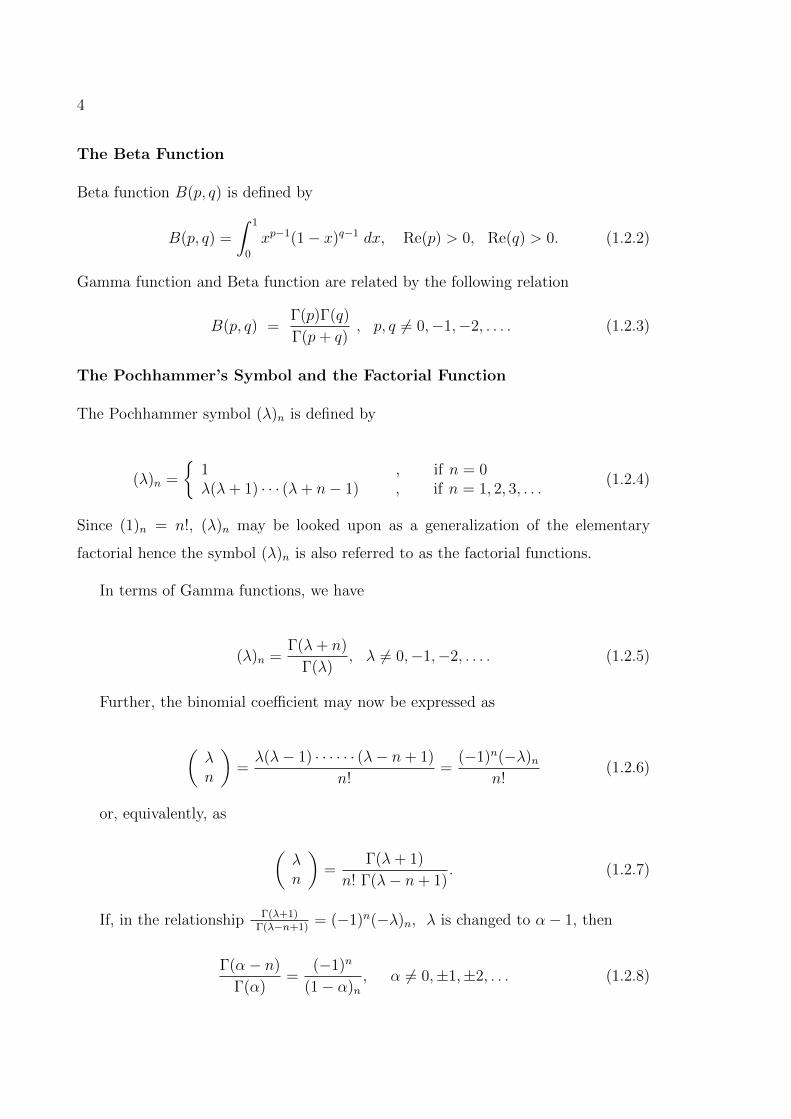
The Beta Function

Beta function B(p, q) is defined by

B(p, q) =

∫ 1

0

xp−1(1− x)q−1 dx, Re(p) > 0, Re(q) > 0. (1.2.2)

Gamma function and Beta function are related by the following relation

B(p, q) =Γ(p)Γ(q)

Γ(p+ q), p, q 6= 0,−1,−2, . . . . (1.2.3)

The Pochhammer’s Symbol and the Factorial Function

The Pochhammer symbol (λ)n is defined by

(λ)n =

1 , if n = 0λ(λ+ 1) · · · (λ+ n− 1) , if n = 1, 2, 3, . . .

(1.2.4)

Since (1)n = n!, (λ)n may be looked upon as a generalization of the elementary

factorial hence the symbol (λ)n is also referred to as the factorial functions.

In terms of Gamma functions, we have

(λ)n =Γ(λ+ n)

Γ(λ), λ 6= 0,−1,−2, . . . . (1.2.5)

Further, the binomial coefficient may now be expressed as

(λn

)=λ(λ− 1) · · · · · · (λ− n+ 1)

n!=

(−1)n(−λ)nn!

(1.2.6)

or, equivalently, as

(λn

)=

Γ(λ+ 1)

n! Γ(λ− n+ 1). (1.2.7)

If, in the relationship Γ(λ+1)Γ(λ−n+1)

= (−1)n(−λ)n, λ is changed to α− 1, then

Γ(α− n)

Γ(α)=

(−1)n

(1− α)n, α 6= 0,±1,±2, . . . (1.2.8)

5

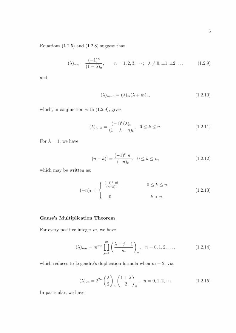
Equations (1.2.5) and (1.2.8) suggest that

(λ)−n =(−1)n

(1− λ)n, n = 1, 2, 3, · · · ; λ 6= 0,±1,±2, . . . (1.2.9)

and

(λ)m+n = (λ)m(λ+m)n, (1.2.10)

which, in conjunction with (1.2.9), gives

(λ)n−k =(−1)k(λ)n

(1− λ− n)k, 0 ≤ k ≤ n. (1.2.11)

For λ = 1, we have

(n− k)! =(−1)k n!

(−n)k, 0 ≤ k ≤ n, (1.2.12)

which may be written as:

(−n)k =

(−1)k n!(n−k)!

, 0 ≤ k ≤ n,

0, k > n.

(1.2.13)

Gauss’s Multiplication Theorem

For every positive integer m, we have

(λ)mn = mmn

m∏j=1

(λ+ j − 1

m

)n

, n = 0, 1, 2, . . . , (1.2.14)

which reduces to Legendre’s duplication formula when m = 2, viz.

(λ)2n = 22n

(λ

2

)n

(1 + λ

2

)n

, n = 0, 1, 2, · · · (1.2.15)

In particular, we have

6

(2n)! = 22n

(1

2

)n

n! and (2n+ 1)! = 22n

(3

2

)n

n!. (1.2.16)

Also [150; p. 86(2)], if m being a positive integer, then

(λ)n−mk =(−1/m)mk(λ)nm∏j=1

(j−λ−nm

)k

, 0 ≤ k ≤ [n/m]. (1.2.17)

For λ = 1, (1.2.17) gives

(n−mk)! =(−1/m)mk n!m−1∏j=0

(j−nm

)k

, 0 ≤ k ≤ [n/m]. (1.2.18)

The Gaussian Hypergeometric Function

The famous German mathematician Gauss introduced the hypergeometric series in

the year 1812.

C.F. Gauss systematically formulated his famous infinite series as follows:

∞∑n=0

(a)n (b)n(c)n

zn

n!= 1 +

ab

c

z

1!+a(a+ 1)b(b+ 1)

c(c+ 1)

z2

2!+ · · · , (1.2.19)

where (a)n = a(a+ 1) · · · (a+ n− 1); (a)0 = 1.

The series is of prime importance to mathematicians and reduces to the elemen-

tary geometric series. Hence it is called the hypergeometric series or, more precisely,

Gauss’s hypergeometric series and usually represented by the symbol 2F1(a, b; c; z),

the well-known Gauss hypergeometric function. The series in (1.2.19) is not defined

if c is zero or negative integer and terminates if either a, b is zero or negative integer.

7

2F1(a, b; c; z) is a solution, regular at z = 0, of the hypergeometric differential

equation

z(1− z)d2u

dz2+ [c− (a+ b+ 1)z]

du

dz− abu = 0, (1.2.20)

where a, b and c are independent of z. This is a homogenous linear differential equa-

tion of the second order and at most three singularities 0, ∞ and 1 which are all

regular.

For |z| < 1 and Re(c) > Re(b) > 0, this function has the integral representation

2F1(a, b; c; z) =Γ(c)

Γ(b)Γ(c− b)

∫ 1

0

tb−1 (1− t)c−b−1(1− zt)−adt. (1.2.21)

The series in (1.2.19) converges for all z, real or complex, such that |z| < 1,

diverges if |z| > 1, and converges absolutely for z = 1 if Re(c− a− b) > 0, and also

when z = −1 if Re(c− a− b) > −1.

Generalized Hypergeometric Function

A natural generalization of the hypergeometric function 2F1 is the generalized hyper-

geometric function, so called pFq which is defined as

pFq

a1, . . . . . . , ap;z

b1, · · · · · · , bq;

=∞∑n=0

(a1)n · · · (ap)n(b1)n · · · (bq)n

zn

n!

=∞∑n=0

[(a)]n[(b)]n

zn

n!, (1.2.22)

where, as usual

(ai)n =Γ(ai + n)

Γ(ai)and [(a)]n =

p∏i=1

(ai)n.

Here p and q are positive integers or zero, the numerator parameters a1, · · · , ap and

the denominator parameters b1, . . . , bq take on complex values, provided that bj 6=

0,−1,−2, . . . ; j = 1, 2, . . . q.

8

An application of elementary ratio test to the power series on the right in (1.2.22)

shows at once that:

(i) if p ≤ q; the series converges for all finite z, that is for | z |<∞;

(ii) if p = q + 1; the series converges for | z |< 1 and diverges for | z |> 1;

(iii) if p > q + 1; the series diverges for z 6= 0. If the series terminates, there is no

question of convergence, and the conclusions (ii) and (iii) do not apply.

(iv) if p = q + 1; the series in (1.2.22) is absolutely convergent on the circle | z |= 1

if Re

(q∑

j=1

bj −p∑

i=1

ai

)> 0.

Also, for p = q + 1, the series is conditionally convergent for | z |= 1, z 6= 1, if

−1 < Re

(q∑j=1

bj −p∑i=1

ai

)≤ 0 and divergent for | z |= 1 if Re

(q∑

j=1

bj −p∑

i=1

ai

)≤ −1.

The generalization of the generalized hypergeometric series pFq is due to Fox

[48] and Wright ([177], [178], [179]) who studied the asymptotic expansion of the

generalized (Wright) hypergeometric function defined by (see [151; p.21])

pΨq

(α1 , A1), ....., (αp , Ap);

(β1 , B1), ....., (βq , Bq);z

=∞∑k=0

p∏j=1

Γ(αj + Ajk)

q∏j=1

Γ(βj +Bjk)

zk

k!, (1.2.23)

where the coefficients A1, · · · , Ap and B1, · · · , Bq are positive real numbers such that

(i) 1 +∑q

j=1Bj −∑p

j=1Aj > 0 and 0 < |z| <∞; z 6= 0;

(ii) 1 +∑q

j=1Bj −∑p

j=1Aj = 0 and 0 < |z| < A1−A1 . . . Ap

−ApB1B1 . . . Bq

Bq .

A special case of (1.2.23) is

pΨq

(α1 , 1), ....., (αp , 1);

(β1 , 1), ....., (βq , 1);z

=

p∏j=1

Γ(αj)

q∏j=1

Γ(βj)pFq

α1, ....., αp ;

β1, ....., βq ;z

,(1.2.24)

where pFq is the generalized hypergeometric series defined by (1.2.22).

9

Confluent Hypergeometric Function

Since, the Gauss function 2F1(a, b; c; z) is a solution of the differential equation

(1.2.20), replacing z by zb

in (1.2.20), we have

z(

1− z

b

) d2u

dz2+

[c−

(1 +

1 + a

b

)z

]du

dz− au = 0. (1.2.25)

Obviously, 2F1(a, b; c; zb) is a solution of (1.2.25).

As b→∞,

lim|b|→∞

2F1(a, b; c;z

b) = 1F1(a; c; z) (1.2.26)

is a solution of differential equation

zd2u

dz2+ (c− z)

du

dz− au = 0. (1.2.27)

The function

1F1(a; c; z) =∞∑n=0

(a)n(c)n

zn

n!(1.2.28)

is called the confluent hypergeometric function or Kummer’s function given by E.E.

Kummer in 1836 [73]. It is also denoted by Humbert’s symbol Φ(a; c; z) and it is

known as confluent hypergeometric function of first kind.

The integral representation of 1F1(a; c; z) is given by

1F1(a; c; z) =Γ(c)

Γ(a)Γ(c− a)

∫ 1

0

ta−1 (1− t)c−a−1eztdt, (1.2.29)

for Re(c) > Re(a) > 0.

The Gauss hypergeometric function 2F1 and the confluent hypergeometric function

1F1 form the core of special functions and include as special cases in most of the

commonly used functions. The 2F1 includes as special cases, most of the classical

orthogonal polynomials, Legendre function, the incomplete beta function etcetera.

On the other hand 0F1 includes as its special cases the Bessel functions.

10

1.3 Hypergeometric Functions of Two Variables

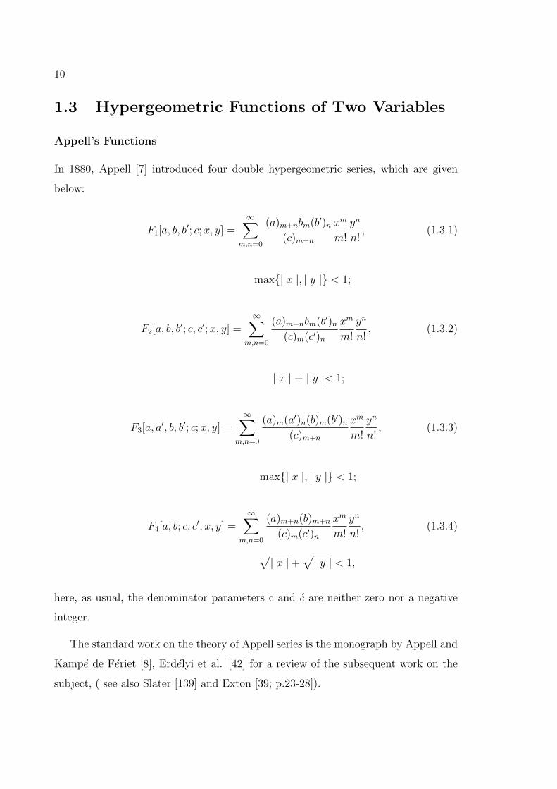
Appell’s Functions

In 1880, Appell [7] introduced four double hypergeometric series, which are given

below:

F1[a, b, b′; c;x, y] =∞∑

m,n=0

(a)m+nbm(b′)n(c)m+n

xm

m!

yn

n!, (1.3.1)

max| x |, | y | < 1;

F2[a, b, b′; c, c′;x, y] =∞∑

m,n=0

(a)m+nbm(b′)n(c)m(c′)n

xm

m!

yn

n!, (1.3.2)

| x | + | y |< 1;

F3[a, a′, b, b′; c;x, y] =∞∑

m,n=0

(a)m(a′)n(b)m(b′)n(c)m+n

xm

m!

yn

n!, (1.3.3)

max| x |, | y | < 1;

F4[a, b; c, c′;x, y] =∞∑

m,n=0

(a)m+n(b)m+n

(c)m(c′)n

xm

m!

yn

n!, (1.3.4)

√| x |+

√| y | < 1,

here, as usual, the denominator parameters c and c are neither zero nor a negative

integer.

The standard work on the theory of Appell series is the monograph by Appell and

Kampe de Feriet [8], Erdelyi et al. [42] for a review of the subsequent work on the

subject, ( see also Slater [139] and Exton [39; p.23-28]).

11

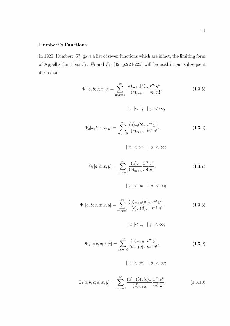
Humbert’s Functions

In 1920, Humbert [57] gave a list of seven functions which are infact, the limiting form

of Appell’s functions F1, F2 and F3; [42; p.224-225] will be used in our subsequent

discussion.

Φ1[a, b; c;x, y] =∞∑

m,n=0

(a)m+n(b)m(c)m+n

xm

m!

yn

n!, (1.3.5)

| x |< 1, | y |<∞;

Φ2[a, b; c;x, y] =∞∑

m,n=0

(a)m(b)n(c)m+n

xm

m!

yn

n!, (1.3.6)

| x |<∞, | y |<∞;

Φ3[a; b;x, y] =∞∑

m,n=0

(a)m(b)m+n

xm

m!

yn

n!, (1.3.7)

| x |<∞, | y |<∞;

Ψ1[a, b; c, d;x, y] =∞∑

m,n=0

(a)m+n(b)m(c)m(d)n

xm

m!

yn

n!, (1.3.8)

| x |< 1, | y |<∞;

Ψ2[a; b, c;x, y] =∞∑

m,n=0

(a)m+n

(b)m(c)n

xm

m!

yn

n!, (1.3.9)

| x |<∞, | y |<∞;

Ξ1[a, b, c; d;x, y] =∞∑

m,n=0

(a)m(b)n(c)m(d)m+n

xm

m!

yn

n!, (1.3.10)

12

| x |< 1, | y |<∞;

Ξ2[a, b; c;x, y] =∞∑

m,n=0

(a)m(b)m(c)m+n

xm

m!

yn

n!, (1.3.11)

| x |< 1, | y |<∞.

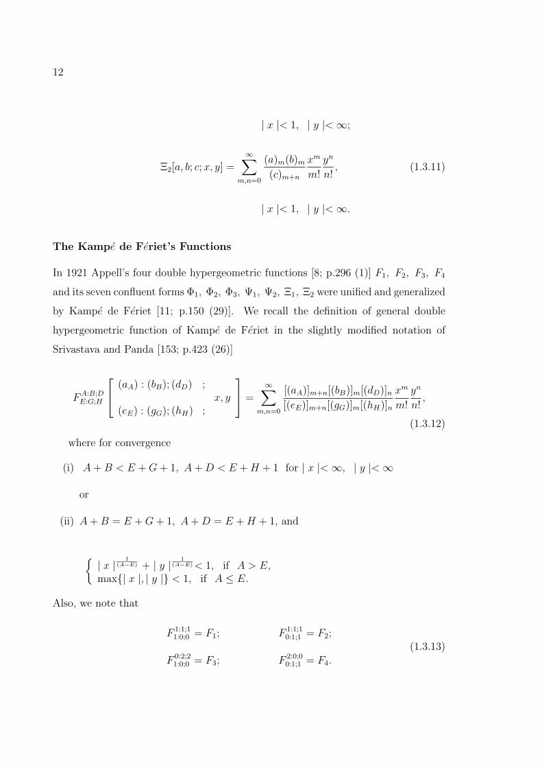
The Kampe de Feriet’s Functions

In 1921 Appell’s four double hypergeometric functions [8; p.296 (1)] F1, F2, F3, F4

and its seven confluent forms Φ1, Φ2, Φ3, Ψ1, Ψ2, Ξ1, Ξ2 were unified and generalized

by Kampe de Feriet [11; p.150 (29)]. We recall the definition of general double

hypergeometric function of Kampe de Feriet in the slightly modified notation of

Srivastava and Panda [153; p.423 (26)]

FA:B;DE:G;H

(aA) : (bB); (dD) ;x, y

(eE) : (gG); (hH) ;

=∞∑

m,n=0

[(aA)]m+n[(bB)]m[(dD)]n[(eE)]m+n[(gG)]m[(hH)]n

xm

m!

yn

n!,

(1.3.12)

where for convergence

(i) A+B < E +G+ 1, A+D < E +H + 1 for | x |<∞, | y |<∞

or

(ii) A+B = E +G+ 1, A+D = E +H + 1, and

| x |

1(A−E) + | y |

1(A−E)< 1, if A > E,

max| x |, | y | < 1, if A ≤ E.

Also, we note that

F 1:1;11:0;0 = F1; F 1:1;1

0:1;1 = F2;

F 0:2;21:0;0 = F3; F 2:0;0

0:1;1 = F4.

(1.3.13)

13

1.4 Hypergeometric Functions of Several Variables

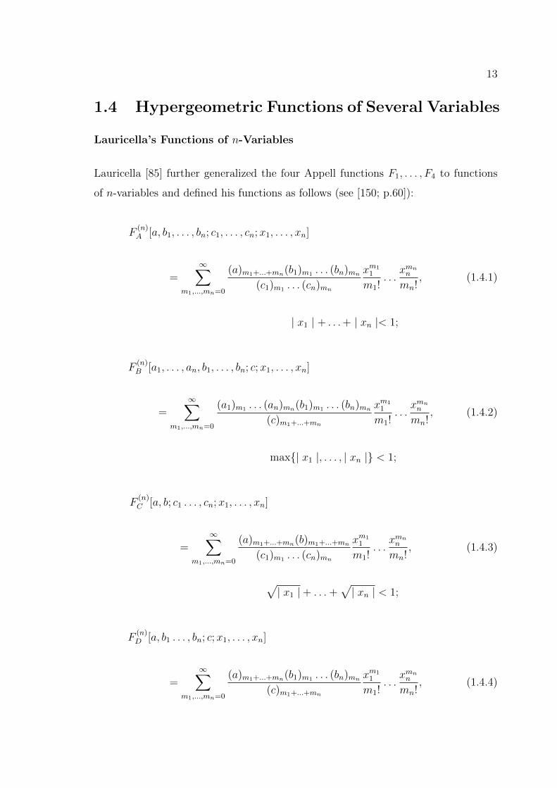
Lauricella’s Functions of n-Variables

Lauricella [85] further generalized the four Appell functions F1, . . . , F4 to functions

of n-variables and defined his functions as follows (see [150; p.60]):

F(n)A [a, b1, . . . , bn; c1, . . . , cn;x1, . . . , xn]

=∞∑

m1,...,mn=0

(a)m1+...+mn(b1)m1 . . . (bn)mn(c1)m1 . . . (cn)mn

xm11

m1!. . .

xmnnmn!

, (1.4.1)

| x1 | + . . .+ | xn |< 1;

F(n)B [a1, . . . , an, b1, . . . , bn; c;x1, . . . , xn]

=∞∑

m1,...,mn=0

(a1)m1 . . . (an)mn(b1)m1 . . . (bn)mn(c)m1+...+mn

xm11

m1!. . .

xmnnmn!

, (1.4.2)

max| x1 |, . . . , | xn | < 1;

F(n)C [a, b; c1 . . . , cn;x1, . . . , xn]

=∞∑

m1,...,mn=0

(a)m1+...+mn(b)m1+...+mn

(c1)m1 . . . (cn)mn

xm11

m1!. . .

xmnnmn!

, (1.4.3)

√| x1 |+ . . .+

√| xn | < 1;

F(n)D [a, b1 . . . , bn; c;x1, . . . , xn]

=∞∑

m1,...,mn=0

(a)m1+...+mn(b1)m1 . . . (bn)mn(c)m1+...+mn

xm11

m1!. . .

xmnnmn!

, (1.4.4)

14

max| x1 |, . . . , | xn | < 1;

clearly, we have,

F(2)A = F2; F

(2)B = F3; F

(2)C = F4; F

(2)D = F1 (1.4.5)

and

F(1)A = F

(1)B = F

(1)C = F

(1)D = 2F1. (1.4.6)

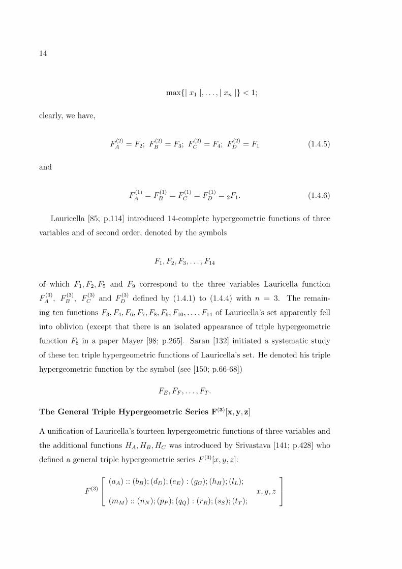
Lauricella [85; p.114] introduced 14-complete hypergeometric functions of three

variables and of second order, denoted by the symbols

F1, F2, F3, . . . , F14

of which F1, F2, F5 and F9 correspond to the three variables Lauricella function

F(3)A , F

(3)B , F

(3)C and F

(3)D defined by (1.4.1) to (1.4.4) with n = 3. The remain-

ing ten functions F3, F4, F6, F7, F8, F9, F10, . . . , F14 of Lauricella’s set apparently fell

into oblivion (except that there is an isolated appearance of triple hypergeometric

function F8 in a paper Mayer [98; p.265]. Saran [132] initiated a systematic study

of these ten triple hypergeometric functions of Lauricella’s set. He denoted his triple

hypergeometric function by the symbol (see [150; p.66-68])

FE, FF , . . . , FT .

The General Triple Hypergeometric Series F(3)[x,y, z]

A unification of Lauricella’s fourteen hypergeometric functions of three variables and

the additional functions HA, HB, HC was introduced by Srivastava [141; p.428] who

defined a general triple hypergeometric series F (3)[x, y, z]:

F (3)

(aA) :: (bB); (dD); (eE) : (gG); (hH); (lL);x, y, z

(mM) :: (nN); (pP ); (qQ) : (rR); (sS); (tT );

15

=∞∑

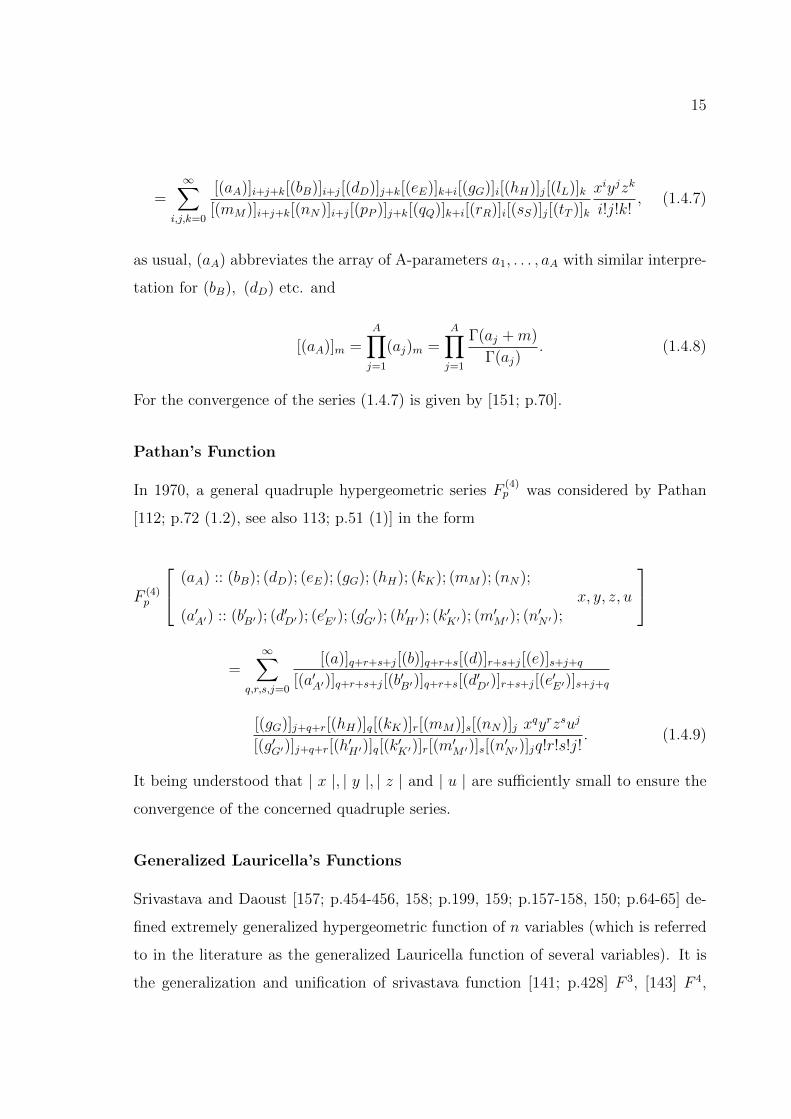
i,j,k=0

[(aA)]i+j+k[(bB)]i+j[(dD)]j+k[(eE)]k+i[(gG)]i[(hH)]j[(lL)]k[(mM)]i+j+k[(nN)]i+j[(pP )]j+k[(qQ)]k+i[(rR)]i[(sS)]j[(tT )]k

xiyjzk

i!j!k!, (1.4.7)

as usual, (aA) abbreviates the array of A-parameters a1, . . . , aA with similar interpre-

tation for (bB), (dD) etc. and

[(aA)]m =A∏j=1

(aj)m =A∏j=1

Γ(aj +m)

Γ(aj). (1.4.8)

For the convergence of the series (1.4.7) is given by [151; p.70].

Pathan’s Function

In 1970, a general quadruple hypergeometric series F(4)p was considered by Pathan

[112; p.72 (1.2), see also 113; p.51 (1)] in the form

F (4)p

(aA) :: (bB); (dD); (eE); (gG); (hH); (kK); (mM); (nN);

(a′A′) :: (b′B′); (d′D′); (e′E′); (g′G′); (h′H′); (k′K′); (m′M ′); (n′N ′);x, y, z, u

=∞∑

q,r,s,j=0

[(a)]q+r+s+j[(b)]q+r+s[(d)]r+s+j[(e)]s+j+q[(a′A′)]q+r+s+j[(b

′B′)]q+r+s[(d

′D′)]r+s+j[(e

′E′)]s+j+q

[(gG)]j+q+r[(hH)]q[(kK)]r[(mM)]s[(nN)]j xqyrzsuj

[(g′G′)]j+q+r[(h′H′)]q[(k

′K′)]r[(m

′M ′)]s[(n

′N ′)]jq!r!s!j!

. (1.4.9)

It being understood that | x |, | y |, | z | and | u | are sufficiently small to ensure the

convergence of the concerned quadruple series.

Generalized Lauricella’s Functions

Srivastava and Daoust [157; p.454-456, 158; p.199, 159; p.157-158, 150; p.64-65] de-

fined extremely generalized hypergeometric function of n variables (which is referred

to in the literature as the generalized Lauricella function of several variables). It is

the generalization and unification of srivastava function [141; p.428] F 3, [143] F 4,

16

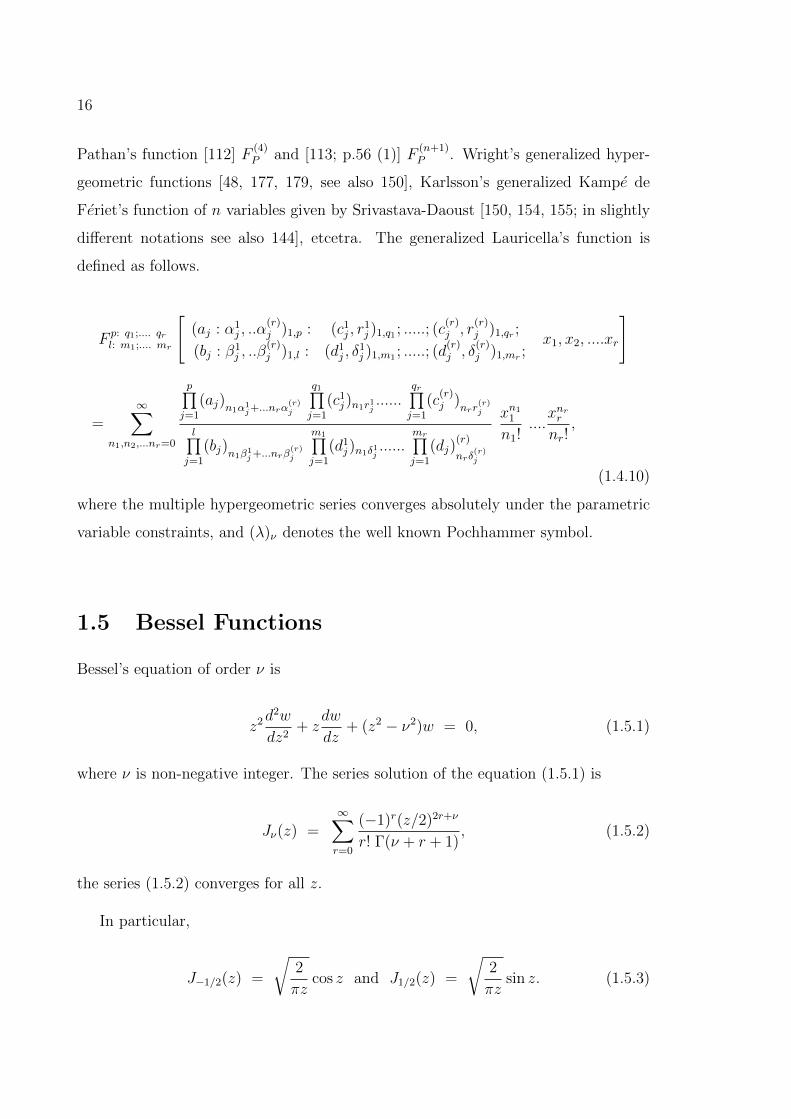
Pathan’s function [112] F(4)P and [113; p.56 (1)] F

(n+1)P . Wright’s generalized hyper-

geometric functions [48, 177, 179, see also 150], Karlsson’s generalized Kampe de

Feriet’s function of n variables given by Srivastava-Daoust [150, 154, 155; in slightly

different notations see also 144], etcetra. The generalized Lauricella’s function is

defined as follows.

F p: q1;.... qrl: m1;.... mr

[(aj : α1

j , ..α(r)j )1,p : (c1

j , r1j )1,q1 ; .....; (c

(r)j , r

(r)j )1,qr ;

(bj : β1j , ..β

(r)j )1,l : (d1

j , δ1j )1,m1 ; .....; (d

(r)j , δ

(r)j )1,mr ;

x1, x2, ....xr

]

=∞∑

n1,n2,...nr=0

p∏j=1

(aj)n1α1j+...nrα

(r)j

q1∏j=1

(c1j)n1r1j

......qr∏j=1

(c(r)j )

nrr(r)j

l∏j=1

(bj)n1β1j+...nrβ

(r)j

m1∏j=1

(d1j)n1δ1j

......mr∏j=1

(dj)(r)

nrδ(r)j

xn11

n1!....xnrrnr!

,

(1.4.10)

where the multiple hypergeometric series converges absolutely under the parametric

variable constraints, and (λ)ν denotes the well known Pochhammer symbol.

1.5 Bessel Functions

Bessel’s equation of order ν is

z2d2w

dz2+ z

dw

dz+ (z2 − ν2)w = 0, (1.5.1)

where ν is non-negative integer. The series solution of the equation (1.5.1) is

Jν(z) =∞∑r=0

(−1)r(z/2)2r+ν

r! Γ(ν + r + 1), (1.5.2)

the series (1.5.2) converges for all z.

In particular,

J−1/2(z) =

√2

πzcos z and J1/2(z) =

√2

πzsin z. (1.5.3)

17

We call Jν(z) as Bessel function of first kind. The generating function for the

Bessel function is given by

exp

[z

2

(t− 1

t

)]=

∞∑ν=−∞

tνJν(z). (1.5.4)

Bessel function is connected with hypergeometric function by the relation

Jν(z) =(z/2)ν

Γ(1 + ν)0F1

;−z2

4ν + 1 ;

. (1.5.5)

Bessel function in terms of confluent hypergeometric function defined by the re-

lation [46; p.333]

Jν(z) =(z/2)ν

Γ(1 + ν)e−iz 1F1

(z +

1

2, 2z + 1; 2iz

). (1.5.6)

Bessel functions are of most frequent use in the theory of integral transform.

An interesting generalization of the Bessel function Jν(z) is due to Wright [180],

who studied the function Jµν (z) defined by

Jµν (z) =∞∑m=0

(−z)m

m! Γ(ν + µm+ 1)(µ > 0; z ∈ C), (1.5.7)

so that, by comparing the definitions (1.5.2) and (1.5.7),

Jν(z) =(z

2

)νJ1ν

(z2

4

). (1.5.8)

Further, another generalization of the Bessel function defined by Pathak [114] is as

follows:

Jµν,λ(z) =∞∑m=0

(−1)m (z/2)ν+2λ+2m

Γ(λ+m+ 1) Γ(ν + λ+ µm+ 1), (1.5.9)

where z ∈ C\(−∞]; µ > 0, ν, λ ∈ C.

So that

J1ν,0(z) = Jν(z) (1.5.10)

18

and

Jµν,0(z) =(z

2

)νJµν

(z2

4

)( µ ∈ <+ ). (1.5.11)

Modified Bessel’s Function

Bessel’s modified differential equation is

z2d2w

dz2+ z

dw

dz− (z2 + ν2)w = 0. (1.5.12)

The series solution of the equation (1.5.12) is

Iν(z) =∞∑r=0

(z/2)2r+ν

r! Γ(ν + r + 1). (1.5.13)

And

Iν(z) =(z/2)ν

Γ(1 + ν)0F1

;z2

4ν + 1 ;

, (1.5.14)

where ν is a non negative integer.

We call Iν(z) as modified Bessel function. The function Iν(z) is related to Jν(z) in

much the same way that the hyperbolic function is related to trigonometric function,

and we have

Iν(z) = i−νJν(iz). (1.5.15)

.

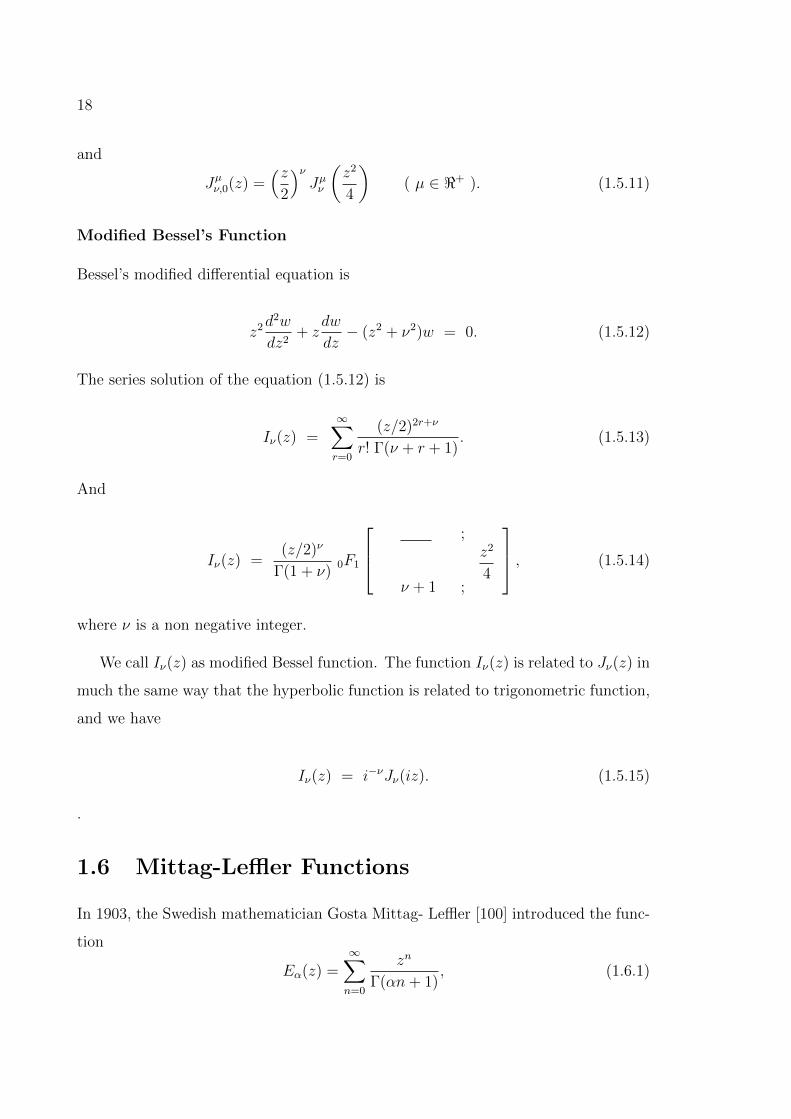
1.6 Mittag-Leffler Functions

In 1903, the Swedish mathematician Gosta Mittag- Leffler [100] introduced the func-

tion

Eα(z) =∞∑n=0

zn

Γ(αn+ 1), (1.6.1)

19

where z is a complex variable and Γ is a Gamma function α ≥ 0. The Mittag-

Leffler function is a direct generalization of exponential function to which it reduces

for α = 1. For 0 < α < 1 it interpolates between the pure exponential and hypergeo-

metric function 11−z . Its importance is realized during the last two decades due to its

involvement in the problems of physics, chemistry, biology, engineering and applied

sciences. Mittag-Leffler function naturally occurs as the solution of fractional order

differential or fractional order integral equation.

The generalization of Eα(z) was studied by Wiman [176] in 1905 and he defined

the function as

Eα,β(z) =∞∑n=0

zn

Γ(αn+ β), (α, β ∈ C, Re(α) > 0, Re(β) > 0), (1.6.2)

which is known as Wiman function.

In 1971, Prabhakar [116] introduced the function Eγα,β(z) in the form of

Eγα,β(z) =

∞∑n=0

(γ)nzn

Γ(αn+ β)n!, (α, β, γ ∈ C, Re(α) > 0, Re(β) > 0, Re(γ) > 0),

(1.6.3)

In 2007, Shukla and Prajapati [148] introduced the function Eγ,qα,β(z) which is

defined for α, β, γ ∈ C, Re(α) > 0, Re(β) > 0, Re(γ) > 0 and q ∈ (0, 1)⋃N as

Eγ,qα,β(z) =

∞∑n=0

(γ)qnzn

Γ(αn+ β)n!, (1.6.4)

In 2009, Tariq O. Salim [134] introduced the function the function Eγ,δα,β(z) which

is defined for α, β, γ, δ ∈ C, Re(α) > 0, Re(β) > 0, Re(γ) > 0, Re(δ) > 0 as

Eγ,δα,β(z) =

∞∑n=0

(γ)nzn

Γ(αn+ β)(δ)n, (1.6.5)

In 2012, a new generalization of Mittag-Leffler function was defined by Salim

[146] as

Eγ,δ,qα,β,p(z) =

∞∑n=0

(γ)qnzn

Γ(αn+ β)(δ)pn, (1.6.6)

where α, β, γ, δ ∈ C, min(Re(α) > 0, Re(β) > 0, Re(γ) > 0, Re(δ) > 0).

20

Recently, Kiryakova [71] defined the multiple (multiindex) Mittag-Leffler function as

follows: Let m > 1 be an integer, ρ1, · · ·ρm > 0 and µ1, · · ·, µm be arbitrary real num-

bers. By means of “multiindices” (ρi)(µi) we introduce the so-called multiindex(m-

tuple) Mittag-Leffler function.

E( 1ρi

),(µi)(z) =

∞∑k=0

zk

Γ(µ1 + kρ1

) · · · Γ(µm + kρm

)(1.6.7)

The relations of multiple (multiindex) Mittag-Leffler function with some known

special functions are as follows:

(i) For m=2, if we put 1ρ1

= α, 1ρ2

= 0 and µ1 = 1, µ2 = 1, in (1.6.7), we have

Eα(z) =∞∑k=0

zk

Γ(1 + αk)(1.6.8)

(ii) For m=2, if we put 1ρ1

= α, 1ρ2

= 0 and µ1 = β, µ2 = 1, in equation (1.6.7), we

have

Eα,β(z) =∞∑k=0

zk

Γ(β + αk)(1.6.9)

(iii) For m=2, if we put 1ρ1

= 1, 1ρ2

= 1 and µ1 = ν + 1, µ2 = 1,and replacing z by

−z24

, in equation (1.6.7), we have (see [71])

E(1,1),(1+ν,1)

(−z2

4

)=

(2

z

)νJν(z) (1.6.10)

where Jν(z) is a Bessel function of first kind (see [131],[150]).

(iv) For m=2, if we put 1ρ1

= 1, 1ρ2

= 1 and µ1 = 3−ν+µ2

, µ2 = 3+ν+µ2

, and replacing z

by −z2

4, in equation (1.6.7), we have (see [71])

E(1,1),( 3−ν+µ2

, 3+ν+µ2

)

(−z2

4

)=

1

zµ+14Sµ,ν(z) (1.6.11)

where Sµ,ν(z) is a Struve function (see [131],[150]).

21

(v) For m=2, if we put 1ρ1

= 1, 1ρ2

= 1 and µ1 = 32, µ2 = 3+2ν

2, and replacing z by

−z24

, in equation (1.6.7), we have (see [71])

E(1,1),( 32, 3+2ν

2)

(−z2

4

)=

1

zµ+14Hν(z) (1.6.12)

where Hν(z) is a Lommel function (see [131],[150]).

1.7 Whittaker Functions

A linear homogeneous ordinary differential equation of the second order

d2w

dz2+

(1/4−m2

z2+k

z− 1

4

)w = 0, (1.7.1)

is called the Whittaker equation. The functions Mk,m(z) and Wk,m(z) are the solu-

tions of this Whittaker equation.

In terms of Confluent hypergeometric functions, the Whittaker functions are defined

as (see Whittaker and Watson [181])

Mk,m(z) = z1/2+me−z/2 Φ

(1

2+m− k, 1 + 2m; z

)(1.7.2)

and

Wk,m(z) = z1/2+me−z/2 Ψ

(1

2+m− k, 1 + 2m; z

). (1.7.3)

When | arg(z) |< 3π/2 and 2m is not an integer

Wk,m(z) =Γ(−2m)

Γ(

12−m− k

)Mk,m(z) +Γ(2m)

Γ(

12

+m− k)Mk,−m(z), (1.7.4)

when | arg(−z) |< 3π/2 and 2m is not an integer

W−k,m(z) =Γ(−2m)

Γ(

12−m− k

)M−k,m(−z) +Γ(2m)

Γ(

12

+m+ k)M−k,−m(−z). (1.7.5)

Whittaker functions satisfy the recurrence relations

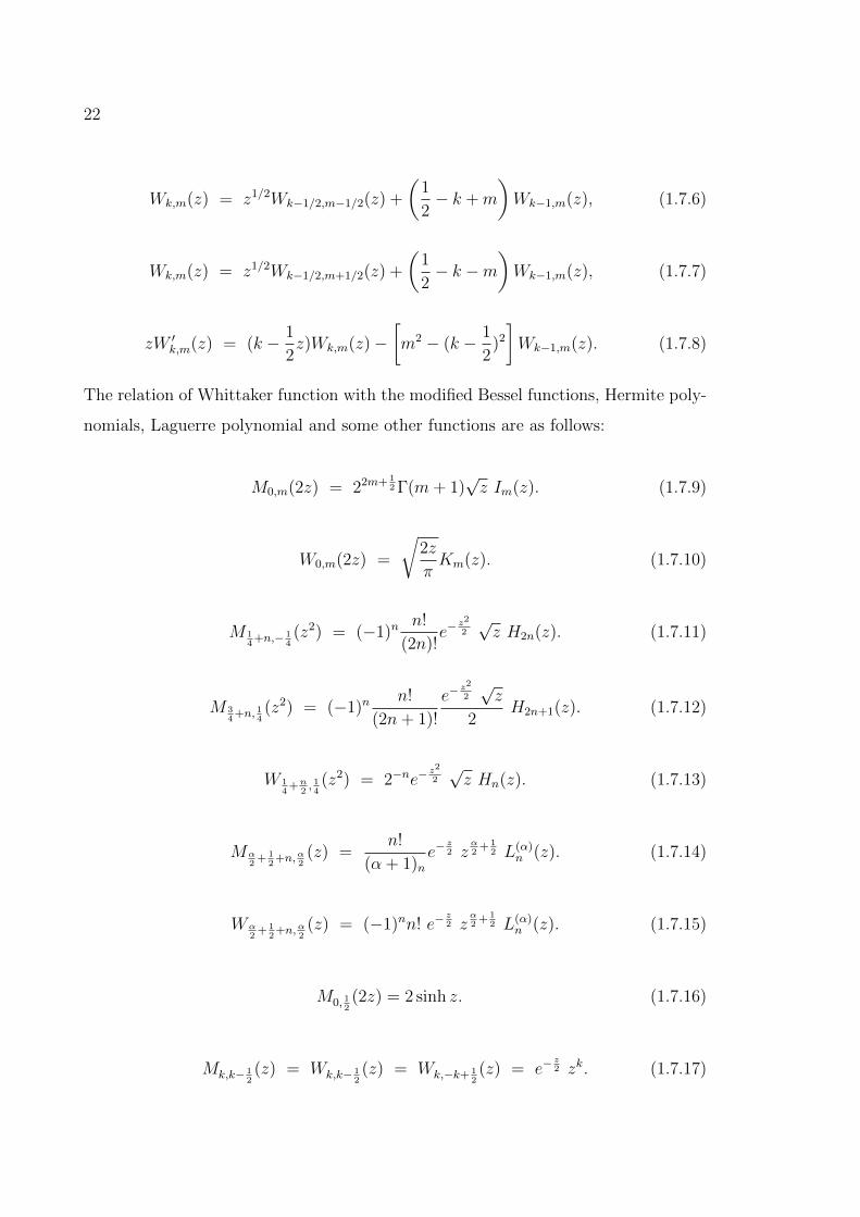
22

Wk,m(z) = z1/2Wk−1/2,m−1/2(z) +

(1

2− k +m

)Wk−1,m(z), (1.7.6)

Wk,m(z) = z1/2Wk−1/2,m+1/2(z) +

(1

2− k −m

)Wk−1,m(z), (1.7.7)

zW ′k,m(z) = (k − 1

2z)Wk,m(z)−

[m2 − (k − 1

2)2

]Wk−1,m(z). (1.7.8)

The relation of Whittaker function with the modified Bessel functions, Hermite poly-

nomials, Laguerre polynomial and some other functions are as follows:

M0,m(2z) = 22m+ 12 Γ(m+ 1)

√z Im(z). (1.7.9)

W0,m(2z) =

√2z

πKm(z). (1.7.10)

M 14

+n,− 14(z2) = (−1)n

n!

(2n)!e−

z2

2√z H2n(z). (1.7.11)

M 34

+n, 14(z2) = (−1)n

n!

(2n+ 1)!

e−z2

2√z

2H2n+1(z). (1.7.12)

W 14

+n2, 14(z2) = 2−ne−

z2

2√z Hn(z). (1.7.13)

Mα2

+ 12

+n,α2(z) =

n!

(α + 1)ne−

z2 z

α2

+ 12 L(α)

n (z). (1.7.14)

Wα2

+ 12

+n,α2(z) = (−1)nn! e−

z2 z

α2

+ 12 L(α)

n (z). (1.7.15)

M0, 12(2z) = 2 sinh z. (1.7.16)

Mk,k− 12(z) = Wk,k− 1

2(z) = Wk,−k+ 1

2(z) = e−

z2 zk. (1.7.17)

23

Mk,−k− 12(z) = e

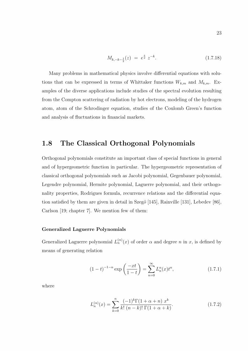
z2 z−k. (1.7.18)

Many problems in mathematical physics involve differential equations with solu-

tions that can be expressed in terms of Whittaker functions Wk,m and Mk,m. Ex-

amples of the diverse applications include studies of the spectral evolution resulting

from the Compton scattering of radiation by hot electrons, modeling of the hydrogen

atom, atom of the Schrodinger equation, studies of the Coulomb Green’s function

and analysis of fluctuations in financial markets.

1.8 The Classical Orthogonal Polynomials

Orthogonal polynomials constitute an important class of special functions in general

and of hypergeometric function in particular. The hypergeometric representation of

classical orthogonal polynomials such as Jacobi polynomial, Gegenbauer polynomial,

Legendre polynomial, Hermite polynomial, Laguerre polynomial, and their orthogo-

nality properties, Rodrigues formula, recurrence relations and the differential equa-

tion satisfied by them are given in detail in Szego [145], Rainville [131], Lebedev [86],

Carlson [19; chapter 7]. We mention few of them:

Generalized Laguerre Polynomials

Generalized Laguerre polynomial L(α)n (x) of order α and degree n in x, is defined by

means of generating relation

(1− t)−1−α exp

(−xt1− t

)=∞∑n=0

Lαn(x)tn, (1.7.1)

where

L(α)n (x) =

n∑k=0

(−1)kΓ(1 + α + n) xk

k! (n− k)! Γ(1 + α + k). (1.7.2)

24

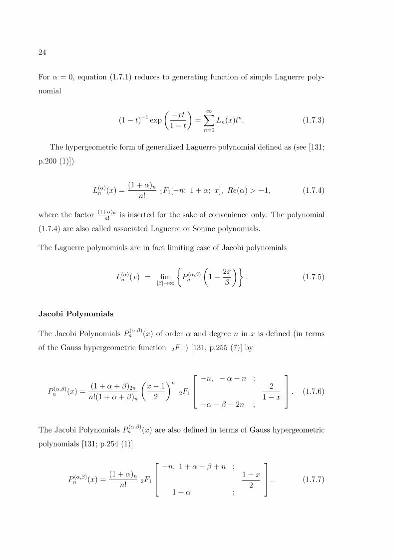
For α = 0, equation (1.7.1) reduces to generating function of simple Laguerre poly-

nomial

(1− t)−1 exp

(−xt1− t

)=∞∑n=0

Ln(x)tn. (1.7.3)

The hypergeometric form of generalized Laguerre polynomial defined as (see [131;

p.200 (1)])

L(α)n (x) =

(1 + α)nn!

1F1[−n; 1 + α; x], Re(α) > −1, (1.7.4)

where the factor (1+α)nn!

is inserted for the sake of convenience only. The polynomial

(1.7.4) are also called associated Laguerre or Sonine polynomials.

The Laguerre polynomials are in fact limiting case of Jacobi polynomials

L(α)n (x) = lim

|β|→∞

P (α,β)n

(1− 2x

β

). (1.7.5)

Jacobi Polynomials

The Jacobi Polynomials P(α,β)n (x) of order α and degree n in x is defined (in terms

of the Gauss hypergeometric function 2F1 ) [131; p.255 (7)] by

P (α,β)n (x) =

(1 + α + β)2n

n!(1 + α + β)n

(x− 1

2

)n2F1

−n, − α− n ;2

1− x−α− β − 2n ;

. (1.7.6)

The Jacobi Polynomials P(α,β)n (x) are also defined in terms of Gauss hypergeometric

polynomials [131; p.254 (1)]

P (α,β)n (x) =

(1 + α)nn!

2F1

−n, 1 + α + β + n ;1− x

21 + α ;

. (1.7.7)

25

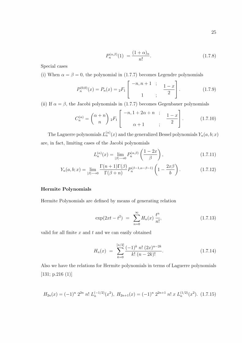
P (α,β)n (1) =

(1 + α)nn!

. (1.7.8)

Special cases

(i) When α = β = 0, the polynomial in (1.7.7) becomes Legendre polynomials

P (0,0)n (x) = Pn(x) = 2F1

−n, n+ 1 ;

1 ;

1− x2

. (1.7.9)

(ii) If α = β, the Jacobi polynomials in (1.7.7) becomes Gegenbauer polynomials

C(α)n =

(α + n

n

)2F1

−n, 1 + 2α + n ;

α + 1 ;

1− x2

. (1.7.10)

The Laguerre polynomials L(α)n (x) and the generalized Bessel polynomials Yn(a, b;x)

are, in fact, limiting cases of the Jacobi polynomials

L(α)n (x) = lim

|β|−→0P (α,β)n

(1− 2x

β

), (1.7.11)

Yn(a, b;x) = lim|β|−→0

Γ(n+ 1)Γ(β)

Γ(β + n)P (β−1,α−β−1)n

(1− 2xβ

b

). (1.7.12)

Hermite Polynomials

Hermite Polynomials are defined by means of generating relation

exp(2xt− t2) =∞∑n=0

Hn(x)tn

n!, (1.7.13)

valid for all finite x and t and we can easily obtained

Hn(x) =

[n/2]∑k=0

(−1)k n! (2x)n−2k

k! (n− 2k)!. (1.7.14)

Also we have the relations for Hermite polynomials in terms of Laguerre polynomials

[131; p.216 (1)]

H2n(x) = (−1)n 22n n! L(−1/2)n (x2), H2n+1(x) = (−1)n 22n+1 n! x L(1/2)

n (x2). (1.7.15)

26

Legendre Polynomials

When α = β = 0 in equation (1.7.7), we get the Legendre polynomials Pn(x) [131;

p.166 (21)]

Pn(x) = 2F1

[−n, n+ 1; 1;

1− x2

]. (1.7.16)

The Legendre polynomial Pn(x) is generated by means of generating relation

(1− 2xt+ t2)−12 =

∞∑n=0

Pn(x)tn. (1.7.17)

Gegenbauer Polynomials

When α = β, the Jacobi polynomials in (1.7.7) reduces to Gegenbauer polynomials

Cνn(x), given by

Cνn(x) =

(2ν)nn!

2F1

−n, 2ν + n ;1− x

2ν + 1

2;

. (1.7.18)

Cγn(1) =

(2γ)nn!

. (1.7.19)

Gegenbauer polynomial is defined by means of generating relation [131; p.276 (1)]

(1− 2xt+ t2)−ν =∞∑n=0

Cνn(x)tn. (1.7.20)

We have some important polynomials which can be expressed in terms of Gegen-

bauer polynomial for different values of ν, as follows:

C12n (x) = Pn(x), (1.7.21)

C1n(x) =

(n+ 1)!

(32)n

P( 12, 12

)n (x) = Un(x), (1.7.22)

27

where Pn(x) is Legendre polynomial and Un(x) is Tchebycheff polynomial of second

kind respectively.

The Gegenbauer polynomials is an important class of orthogonal polynomials

which is the generalization of Legendre and Tchebycheff polynomials of second kind

Un(x). It is also known that the Gegenbauer and Ultraspherical polynomials are

essentially equivalent (see [131; p.277 (4),(5)]).

Cνn(x) =

(2ν)n(ν + 1

2)nP

(ν− 12, ν− 1

2)

n (x), (1.7.23)

P (α,α)n (x) =

(1 + α)nCα+ 1

2n (x)

(1 + 2α)n. (1.7.24)

Tchebycheff Polynomials

When α = β = −12

or α = β = 12, the Jacobi polynomials in (1.7.7) reduces to the

Tchebycheff polynomial of the first and second kind Tn(x) and Un(x) [150; p.36 (38)]

given by

Tn(x) =n!

(12)n

P(− 1

2,− 1

2)

n (x), (1.7.25)

Un(x) =(n+ 1)!

(32)n

P( 12, 12

)n (x), (1.7.26)

Tchebycheff polynomial of the first and second kind is defined by means of gen-

erating relation [131; p.276 (1)]

(1− xt)(1− 2xt+ t2)−1 =∞∑n=0

Tn(x)tn. (1.7.27)

(1− 2xt+ t2)−1 =∞∑n=0

Un(x)tn. (1.7.28)

28

Lagrange’s Polynomials

The Lagrange polynomial is defined by means of generating function [44; p.267 see

also 150; p.85 (25)].

∞∑n=0

g(α,β)n (x, y)tn = (1− xt)−α(1− yt)−β (1.7.29)

where

g(α,β)n (x, y) = (y − x)nP (−α−n,−β−n)

n

(x+ y

x− y

)(1.7.30)

Bernoulli Polynomials

Much good has come from the study of Bn(x) defined by(t

et − 1

)=∞∑n=0

Bn(x)tn

n!, (1.7.31)

particularly in the theory of numbers. The Bn(x) of (1.7.31) are the Bernoulli poly-

nomials, which have been generalized in numerous directions. See Erdelyi [42] and

[43]. The Bn(x)/n! are of Sheffer A-type zero, from which fact various interesting

properties may be obtained. It is also a simple matter to show that

Bn(x+ 1)−Bn(x) = nxn−1, (1.7.32)

Bn(x+ 1) + 1 +B(x)n, (1.7.33)

Bn(1− x) = (−1)nBn(x), (1.7.34)

One definition of Bernoulli number Bn is

Bn = Bn(0). (1.7.35)

It follows that

Bn(x) + B + xn (1.7.36)

and

Bn(1) = Bn, n ≥ 2, B1(1) = 1 +B1. (1.7.37)

29

Sincet

et − 1= −t+

−te−t − 1

,

B1 is the only nonzero Bernoulli number with odd index. Thus the generating relation

t

et − 1=∞∑n=0

Bntn

n!(1.7.38)

may also be writtent

et − 1= B0 +B1t+

∞∑n=1

B2nt2n

(2n)!, (1.7.39)

in which B0 = 1, B1 = −12, etc.

Euler Polynomials

The polynomials En(x) defined by(2

et + 1

)ext =

∞∑n=0

En(x)tn

n!(1.7.40)

are called the Euler polynomials, and the numbers

En = 2nEn

(1

2

)(1.7.41)

are called the Euler numbers. The polynomials En(x)/n! are of Sheffer A-type zero.

It is not difficult to obtain such results as

En(x+ 1) + En(x) = 2xn, (1.7.42)

En(1− x) = (−1)nEn(x), (1.7.43)

En(x+ 1) + 1 + E(x)n, (1.7.44)

nEn−1(x) = 2Bn(x)− 2n+1Bn

(x2

). (1.7.45)

Since the Euler numbers defined in (1.7.41) have the generating relation

∞∑n=0

Entn

n!=

2et

e2t + 1=

2e−t

1 + e−2t, (1.7.46)

it follows that E2n+1 = 0.

30

Genocchi Polynomials

In the complex plane, the Genocchi numbers, named after Angelo Genocchi, are a

sequence of integers that defined by the exponential generating function:(2t

et + 1

)= eGt =

∞∑n=0

Gntn

n!, (|t| < π) (1.7.47)

with the usual convention about replacing Gn by Gn, is used. When we multiply

with ext in the left hand side of (1.7.47), then we have

(2t

et + 1

)ext =

∞∑n=0

Gn(x)tn

n!, (|t| < π) (1.7.48)

where Gn(x) are called the Genocchi polynomials, It follows from (1.7.45) that G1 =

1, G2 = −1, G3 = 0, G4 = 1, G5 = 0, G6 = −3, G7 = 0, G8 = 17, · · · , and

G2n+1 = 0 for n ∈ N .

Legendre Function

P µν (z) =

1

Γ(1− µ)

(z + 1

z − 1

)µ/22F1

−ν, ν + 1 ;1− z

21− µ ;

. (1.7.49)

The function P µν (z) is known as the Legendre function of first kind [42]. It is one of

valued and regular in z-plane supposed cut along the real axis from 1 to −∞.

Other familiar generalizations (and unifications) of the various polynomials are

studied by Srivastava and Singhal [163], Srivastava and Joshi [164], Srivastava and

Panda [153], Srivastava and Pathan [155] and Shahabuddin [135].

1.9 Generating Functions

The name ‘generating function’ was introduced by Laplace in 1812. Since then the

theory of generating functions has been developed into various directions and found

wide applications in various branches of science and technology. A generating function

31

may be used to define a set of functions, to determine a differential recurrence relation

or a pure recurrence relation, to evaluate certain integrals, etc.

Linear Generating Functions

Consider a two-variable function F (x, t) which possesses a formal (not necessarily

convergent for t 6= 0) power series expansion in t such that

F (x, t) =∞∑n=0

fn(x)tn, (1.8.1)

where each member of the coefficient set fn(x)∞n=0 is independent of t. Then the

expansion (1.8.1) of F (x, t) is said to have generated the set fn(x) and F (x, t)

is called a linear generating function (or, simply, generating function) for the set

fn(x).

The definition (1.8.1) may be extended slightly to include a generating function

of the type:

G(x, t) =∞∑n=0

cngn(x)tn, (1.8.2)

where the sequence cn(x)∞n=0 may contain the parameter of the set gn(x), but is

independent of x and t.

Bilinear and Bilateral Generating Functions

If a three-variable function F (x, y, t) possesses a formal power series expansions in t

such that

F (x, y, t) =∞∑n=0

γnfn(x)fn(y)tn, (1.8.3)

where the sequence γn is independent of x, y and t, then F (x, y, t) is called a

bilinear generating function for the set fn(x).

Now suppose that a three-variable function H(x, y, t) has a formal power series

expansion in t such that

32

H(x, y, t) =∞∑n=0

hnfn(x)gn(y)tn, (1.8.4)

where the sequence hn is independent of x, y and t, and the sets of functions

fn(x)∞n=0 and gn(x)∞n=0 are different then Hn(x, y, t) is called a bilateral generating

function for the set fn(x) or gn(x).

The above definition of a bilateral generating function, used earlier by McBride [99]

and Rainville [131] may be extended to include bilateral generating functions of the

type:

H(x, y, t) =∞∑n=0

γnfα(n)(x)gβ(n)(y)tn, (1.8.5)

where the sequence γn is independent of x, y and t, the sets of functions fn(x)∞n=0

and gn(x)∞n=0 are different, and α(n) and β(n) are functions of n which are not nec-

essarily equal.

Multivariable Generating Functions

In each of the above definition, the sets generated are functions of only one variable.

Suppose now that G(x1, ..., xr; t) is a function of r + 1 variables, which has a formal

expansion in power of t, such that

G(x1, ..., xr; t) =∞∑n=0

cngn(x1, ..., xr)tn, (1.8.6)

where the sequence cn(x) is independent of the variables x1, ..., xr and t. Then we

shall say that G(x1, ..., xr; t) is generating function for the set gn(x1, ..., xr)∞n=0 corre-

sponding to the nonzero coefficient cn.

33

Multilinear and Multilateral Generating Functions

A multivariable generating function given by (1.8.6), is said to be a multilinear gen-

erating function if

gn(x1, ..., xr) = gα1(n)(x1)...gαr(n)(xr), (1.8.7)

where α1(n), ..., αr(n) are functions of n which are not necessarily equal. More gen-

erally, if the functions occurring on the right-hand side of (1.8.7) are all different,

the multivariable generating function (1.8.7) will be called as multilateral generating

function.

Application of Generating Functions

A generating function may be used to define a set of functions, to determine a differ-

ential recurrence relation or a pure recurrence relation, to evaluate certain integrals,

etc.

We define Legendre polynomials Pn(x), Bessel’s functions Jn(x), Hermite polyno-

mials Hn(x), Laguerre polynomials Ln(x), associated Laguerre polynomials Lαn(x),

Tchebicheff polynomials of first and second kinds Tn(x) and Un(x), Gegenbauer or

Ultraspherical polynomials Cνn(x) and Jacobi polynomials P

(α,β)n (x) by mean of the

generating relations.

1.10 Integral Transforms

Integral transforms play an important role in various fields of physics. The method of

solution of problems arising in physics lie at the heart of the use of integral transform.

Let f(t) be a real or complex valued function of real variable t, defined on interval

a ≤ t ≤ b, which belongs to a certain specified class of functions and let F (p, t)

be a definite function of p and t, where p is a complex quantity, whose domain is

prescribed, then the integral equation

34

φ[f(t); p] =

∫ b

a

F (p, t)f(t) dt, (1.9.1)

where the class of functions to which f(t) belongs and the domain of p are so pre-

scribed that the integral on the right exists.

F (p, t) is called the kernel of the transform φ[f(t), p], if we can define an integral

equation

f(t) =

∫ d

c

F (t)φ[f(t), p] dp, (1.9.2)

then (1.9.2) defines the inverse transform for (1.9.1). By given different values to

the function F (p, t), different integral transforms like Fourier, Laplace, Hankel and

Mellin transforms etc. are defined by various mathematicians.

Fourier Transform

We call

F [f(x); ξ] = (2π)−1/2

∫ ∞−∞

f(x)eiξx dx, (1.9.3)

the Fourier transform of f(x) and regard x as complex variable.

Laplace Transform

We call

L[f(t); p] =

∫ ∞0

f(t)e−pt dt, (1.9.4)

the Laplace transform of f(t) and regard p as complex variable.

Hankel Transform

We call

Hν [f(t); ξ] =

∫ ∞0

f(t) tJν(ξt) dt, (1.9.5)

35

the Hankel transform of f(t) and regard ξ as complex variable.

Mellin Transform

We call

M[f(x); s] =

∫ ∞0

f(x) xs−1 dx, (1.9.6)

the Mellin transform of f(x) and regard s as complex variable.

The most complete set of integral transforms are given in Erdelyi et al. [45, 46]

Ditkin and Prudnikov [35] and Prudnikov et al. [129, 130].

Chapter 2

On Certain Mixed GeneratingFunctions Involving the Product ofJacobi Polynomials

2.1 Introduction

In the usual notation, let

L(α)n (x) =

n∑r=0

(n+ αn− r

)(−x)r

r!(2.1.1)

denote the Laguerre polynomial of order α and degree n in its arguments x defined

by (1.7.2).

In recent years, several formulae have been given which express the product of

two Laguerre polynomials as a sum of involving these polynomials. In 1936, Bailey

[12] give a result which is associated with polynomials with the same order and

exponent but different argument is

L(α)n (x)L(α)

n (y) =Γ(1 + α + n)

n!

n∑r=0

(xy)rL(α+2r)n−r (x+ y)

r!(1 + α + r)(2.1.2)

A formula involving two Laguerre polynomials with the same arguments and exponent

but with different order obtained by Howell and Erdelyi in (1937), is

L(α)n (x)L(α)

n (y) =Γ(1 + α +m)Γ(1 + α + n)

Γ(1 + α +m+ n)

36

37

×min(m,n)∑r=0

(m+ n− 2r)!

r!(m− r)!(n− r)!Γ(1 + α + r)x2rL

(α+2r)m+n−2r(x) (2.1.3)

Watson [173] has obtained a formula for the product of two Laguerre polynomials

with the same arguments and exponents but with different order as

L(α)n (x)L(α)

n (y) =

2min(m,n)∑r=0

CrL(α)m+n−r(x) (2.1.4)

where the coefficients Cr are given in term of a series 3F2(1) and Erdelyi [40] has

shown how equivalent formula can be obtained from (2.1.2) and his relation

xmL(α+m)n (x) =

Γ(1 + α +m+ n)

n!

m∑r=0

(−m)r(n+ r)!

r!(1 + α + n+ r)L

(α)n+r(x). (2.1.5)

The more general problem of obtaining the expression

L(α1)m1

(Knx) · · ·L(αn)mn (Knx) =

m1+···+mn∑r=0

CrL(α)r (x) (2.1.6)

has been completely solved by Erdelyi, who showed that the coefficients Cr can be

expressed either as a Lauricella’s hypergeometric function FA of (n+ 1) variables or

as n-ple sum. In the case of product of two polynomials, the coefficients Cr is thus

expressed as a double series but it is not all easy to express it as a simple sum.

Bailey [13], give some further expansions for the product of two Laguerre poly-

nomials in which the exponents are different but polynomials have equal order is

L(α)n (x)L(β)

n (x) =Γ(1 + α + n)Γ(1 + β + n)

n!

n∑r=0

(−1)rxrL(α+β+r)r (x)

Γ(1 + α + r)Γ(1 + β + r)(n− r)!(2.1.7)

Now consider a generating function [150; p.106 (11)].

∞∑n=0

P (α−n,β−n)n (x)

tn

(−α− β)n= exp

[−1

2(x+ 1)t

]1F1

− β ;

−α− β ;t

(2.1.8)

38

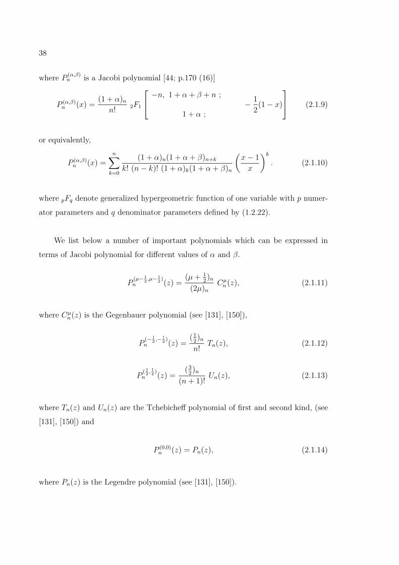
where P(α,β)n is a Jacobi polynomial [44; p.170 (16)]

P (α,β)n (x) =

(1 + α)nn!

2F1

−n, 1 + α + β + n ;

1 + α ;− 1

2(1− x)

(2.1.9)

or equivalently,

P (α,β)n (x) =

n∑k=0

(1 + α)n(1 + α + β)n+k

k! (n− k)! (1 + α)k(1 + α + β)n

(x− 1

x

)k. (2.1.10)

where pFq denote generalized hypergeometric function of one variable with p numer-

ator parameters and q denominator parameters defined by (1.2.22).

We list below a number of important polynomials which can be expressed in

terms of Jacobi polynomial for different values of α and β.

P(µ− 1

2,µ− 1

2)

n (z) =(µ+ 1

2)n

(2µ)nCµn(z), (2.1.11)

where Cµn(z) is the Gegenbauer polynomial (see [131], [150]),

P(− 1

2,− 1

2)

n (z) =(1

2)n

n!Tn(z), (2.1.12)

P( 12, 12

)n (z) =

(32)n

(n+ 1)!Un(z), (2.1.13)

where Tn(z) and Un(z) are the Tchebicheff polynomial of first and second kind, (see

[131], [150]) and

P (0,0)n (z) = Pn(z), (2.1.14)

where Pn(z) is the Legendre polynomial (see [131], [150]).

39

Jacobi polynomial is an important class of orthogonal polynomial which is a gener-

alization of ultraspherical polynomials. This class contains many special functions

commonly encountered in the applications, e.g. Legendre, Gegenbauer, Tchebcheff,

Laguerre and Bessel polynomials.

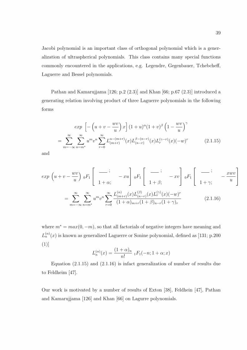
Pathan and Kamarujjama [126; p.2 (2.3)] and Khan [66; p.67 (2.3)] introduced a

generating relation involving product of three Laguerre polynomials in the following

forms

exp[−(u+ v − wv

u

)x]

(1 + u)α(1 + v)β(

1− wv

u

)γ=

∞∑m=−∞

∞∑n=m∗

umvn∞∑r=0

Lα−(m+r)(m+r) (x)L

β−(n−r)(n−r) (x)L(γ−r)

r (x)(−w)r (2.1.15)

and

exp(u+ v − wv

u

)0F1

;

1 + α;− xu

0F1

;

1 + β;− xv

0F1

;

1 + γ;− xwv

u

=

∞∑m=−∞

∞∑n=m∗

umvn∞∑r=0

L(α)(m+r)(x)L

(β)(n−r)(x)L

(γ)r (x)(−w)r

(1 + α)m+r(1 + β)n−r(1 + γ)r(2.1.16)

where m∗ = max(0,−m), so that all factorials of negative integers have meaning and

L(α)n (x) is known as generalized Laguerre or Sonine polynomial, defined as [131; p.200

(1)]

L(α)n (x) =

(1 + α)nn!

1F1(−n; 1 + α;x)

Equation (2.1.15) and (2.1.16) is infact generalization of number of results due

to Feldheim [47].

Our work is motivated by a number of results of Exton [38], Feldhein [47], Pathan

and Kamarujjama [126] and Khan [66] on Lagurre polynomials.

40

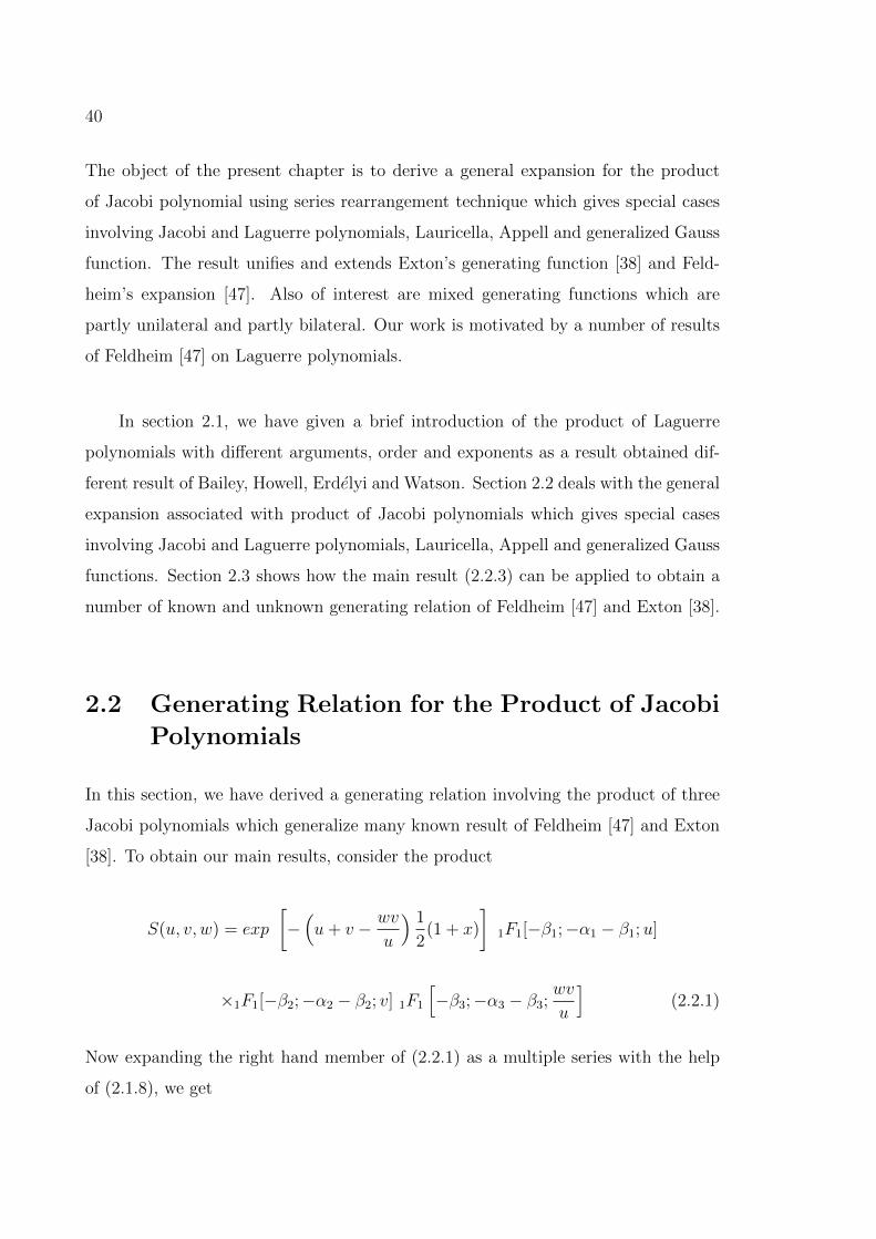
The object of the present chapter is to derive a general expansion for the product

of Jacobi polynomial using series rearrangement technique which gives special cases

involving Jacobi and Laguerre polynomials, Lauricella, Appell and generalized Gauss

function. The result unifies and extends Exton’s generating function [38] and Feld-

heim’s expansion [47]. Also of interest are mixed generating functions which are

partly unilateral and partly bilateral. Our work is motivated by a number of results

of Feldheim [47] on Laguerre polynomials.

In section 2.1, we have given a brief introduction of the product of Laguerre

polynomials with different arguments, order and exponents as a result obtained dif-

ferent result of Bailey, Howell, Erdelyi and Watson. Section 2.2 deals with the general

expansion associated with product of Jacobi polynomials which gives special cases

involving Jacobi and Laguerre polynomials, Lauricella, Appell and generalized Gauss

functions. Section 2.3 shows how the main result (2.2.3) can be applied to obtain a

number of known and unknown generating relation of Feldheim [47] and Exton [38].

2.2 Generating Relation for the Product of Jacobi

Polynomials

In this section, we have derived a generating relation involving the product of three

Jacobi polynomials which generalize many known result of Feldheim [47] and Exton

[38]. To obtain our main results, consider the product

S(u, v, w) = exp

[−(u+ v − wv

u

) 1

2(1 + x)

]1F1[−β1;−α1 − β1;u]

×1F1[−β2;−α2 − β2; v] 1F1

[−β3;−α3 − β3;

wv

u

](2.2.1)

Now expanding the right hand member of (2.2.1) as a multiple series with the help

of (2.1.8), we get

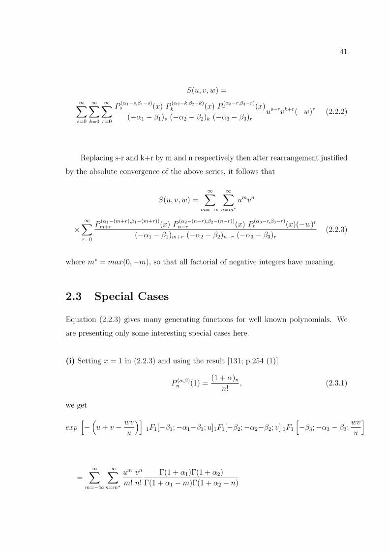
41

S(u, v, w) =

∞∑s=0

∞∑k=0

∞∑r=0

P(α1−s,β1−s)s (x) P

(α2−k,β2−k)k (x) P

(α3−r,β3−r)r (x)

(−α1 − β1)s (−α2 − β2)k (−α3 − β3)rus−rvk+r(−w)r (2.2.2)

Replacing s-r and k+r by m and n respectively then after rearrangement justified

by the absolute convergence of the above series, it follows that

S(u, v, w) =∞∑

m=−∞

∞∑n=m∗

umvn

×∞∑r=0

P(α1−(m+r),β1−(m+r))m+r (x) P

(α2−(n−r),β2−(n−r))n−r (x) P

(α3−r,β3−r)r (x)(−w)r

(−α1 − β1)m+r (−α2 − β2)n−r (−α3 − β3)r(2.2.3)

where m∗ = max(0,−m), so that all factorial of negative integers have meaning.

2.3 Special Cases

Equation (2.2.3) gives many generating functions for well known polynomials. We

are presenting only some interesting special cases here.

(i) Setting x = 1 in (2.2.3) and using the result [131; p.254 (1)]

P (α,β)n (1) =

(1 + α)nn!

, (2.3.1)

we get

exp[−(u+ v − wv

u

)]1F1[−β1;−α1−β1;u]1F1[−β2;−α2−β2; v] 1F1

[−β3;−α3 − β3;

wv

u

]

=∞∑

m=−∞

∞∑n=m∗

um vn

m! n!

Γ(1 + α1)Γ(1 + α2)

Γ(1 + α1 −m)Γ(1 + α2 − n)

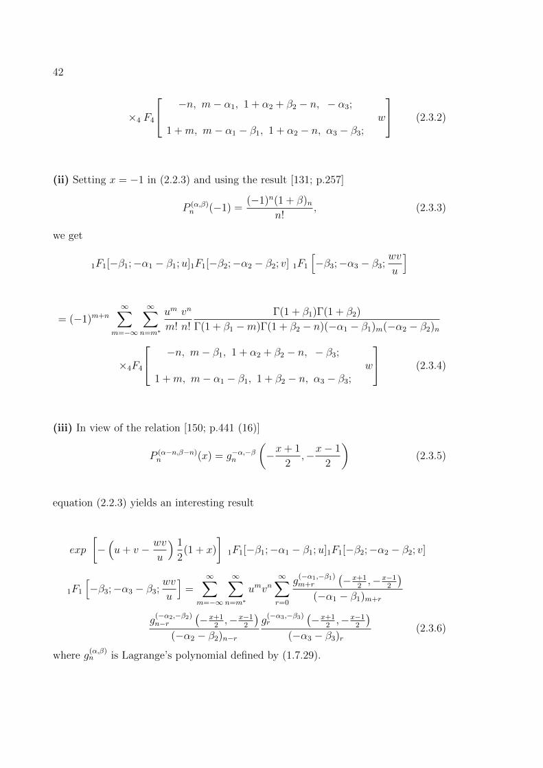
42

×4 F4

−n, m− α1, 1 + α2 + β2 − n, − α3;

1 +m, m− α1 − β1, 1 + α2 − n, α3 − β3;w

(2.3.2)

(ii) Setting x = −1 in (2.2.3) and using the result [131; p.257]

P (α,β)n (−1) =

(−1)n(1 + β)nn!

, (2.3.3)

we get

1F1[−β1;−α1 − β1;u]1F1[−β2;−α2 − β2; v] 1F1

[−β3;−α3 − β3;

wv

u

]

= (−1)m+n

∞∑m=−∞

∞∑n=m∗

um vn

m! n!

Γ(1 + β1)Γ(1 + β2)

Γ(1 + β1 −m)Γ(1 + β2 − n)(−α1 − β1)m(−α2 − β2)n

×4F4

−n, m− β1, 1 + α2 + β2 − n, − β3;

1 +m, m− α1 − β1, 1 + β2 − n, α3 − β3;w

(2.3.4)

(iii) In view of the relation [150; p.441 (16)]

P (α−n,β−n)n (x) = g−α,−βn

(−x+ 1

2,−x− 1

2

)(2.3.5)

equation (2.2.3) yields an interesting result

exp

[−(u+ v − wv

u

) 1

2(1 + x)

]1F1[−β1;−α1 − β1;u]1F1[−β2;−α2 − β2; v]

1F1

[−β3;−α3 − β3;

wv

u

]=

∞∑m=−∞

∞∑n=m∗

umvn∞∑r=0

g(−α1,−β1)m+r

(−x+1

2,−x−1

2

)(−α1 − β1)m+r

g(−α2,−β2)n−r

(−x+1

2,−x−1

2

)(−α2 − β2)n−r

g(−α3,−β3)r

(−x+1

2,−x−1

2

)(−α3 − β3)r

(2.3.6)

where g(α,β)n is Lagrange’s polynomial defined by (1.7.29).

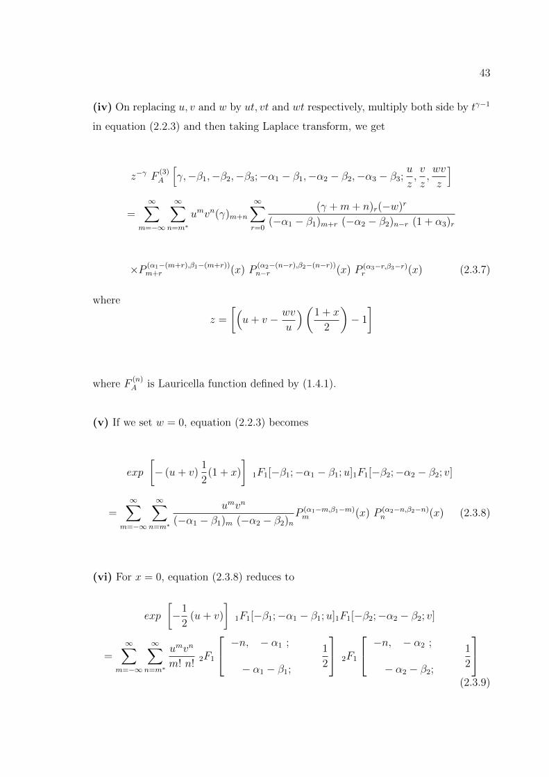
43

(iv) On replacing u, v and w by ut, vt and wt respectively, multiply both side by tγ−1

in equation (2.2.3) and then taking Laplace transform, we get

z−γ F(3)A

[γ,−β1,−β2,−β3;−α1 − β1,−α2 − β2,−α3 − β3;

u

z,v

z,wv

z

]=

∞∑m=−∞

∞∑n=m∗

umvn(γ)m+n

∞∑r=0

(γ +m+ n)r(−w)r

(−α1 − β1)m+r (−α2 − β2)n−r (1 + α3)r

×P (α1−(m+r),β1−(m+r))m+r (x) P

(α2−(n−r),β2−(n−r))n−r (x) P (α3−r,β3−r)

r (x) (2.3.7)

where

z =

[(u+ v − wv

u

)(1 + x

2

)− 1

]

where F(n)A is Lauricella function defined by (1.4.1).

(v) If we set w = 0, equation (2.2.3) becomes

exp

[− (u+ v)

1

2(1 + x)

]1F1[−β1;−α1 − β1;u]1F1[−β2;−α2 − β2; v]

=∞∑

m=−∞

∞∑n=m∗

umvn

(−α1 − β1)m (−α2 − β2)nP (α1−m,β1−m)m (x) P (α2−n,β2−n)

n (x) (2.3.8)

(vi) For x = 0, equation (2.3.8) reduces to

exp

[−1

2(u+ v)

]1F1[−β1;−α1 − β1;u]1F1[−β2;−α2 − β2; v]

=∞∑

m=−∞

∞∑n=m∗

umvn

m! n!2F1

−n, − α1 ;

− α1 − β1;

1

2

2F1

−n, − α2 ;

− α2 − β2;

1

2

(2.3.9)

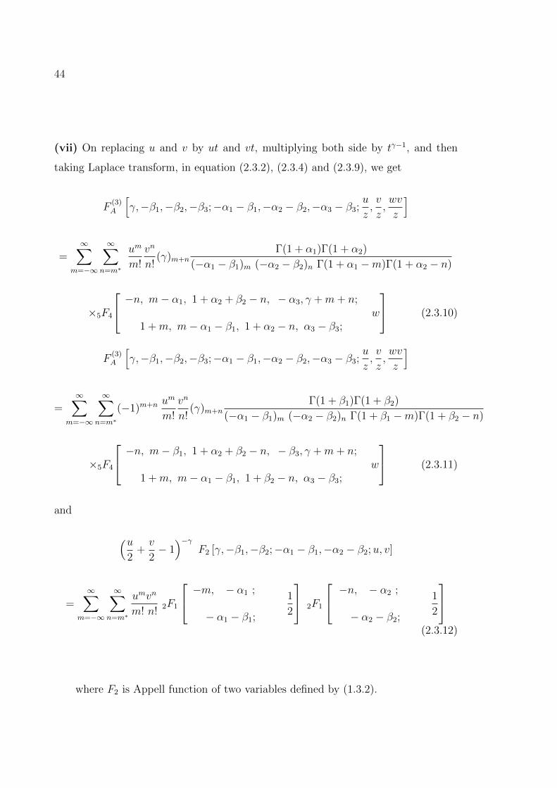
44

(vii) On replacing u and v by ut and vt, multiplying both side by tγ−1, and then

taking Laplace transform, in equation (2.3.2), (2.3.4) and (2.3.9), we get

F(3)A

[γ,−β1,−β2,−β3;−α1 − β1,−α2 − β2,−α3 − β3;

u

z,v

z,wv

z

]

=∞∑

m=−∞

∞∑n=m∗

um

m!

vn

n!(γ)m+n

Γ(1 + α1)Γ(1 + α2)

(−α1 − β1)m (−α2 − β2)n Γ(1 + α1 −m)Γ(1 + α2 − n)

×5F4

−n, m− α1, 1 + α2 + β2 − n, − α3, γ +m+ n;

1 +m, m− α1 − β1, 1 + α2 − n, α3 − β3;w

(2.3.10)

F(3)A

[γ,−β1,−β2,−β3;−α1 − β1,−α2 − β2,−α3 − β3;

u

z,v

z,wv

z

]

=∞∑

m=−∞

∞∑n=m∗

(−1)m+n um

m!

vn

n!(γ)m+n

Γ(1 + β1)Γ(1 + β2)

(−α1 − β1)m (−α2 − β2)n Γ(1 + β1 −m)Γ(1 + β2 − n)

×5F4

−n, m− β1, 1 + α2 + β2 − n, − β3, γ +m+ n;

1 +m, m− α1 − β1, 1 + β2 − n, α3 − β3;w

(2.3.11)

and

(u2

+v

2− 1)−γ

F2 [γ,−β1,−β2;−α1 − β1,−α2 − β2;u, v]

=∞∑

m=−∞

∞∑n=m∗

umvn

m! n!2F1

−m, − α1 ;

− α1 − β1;

1

2

2F1

−n, − α2 ;

− α2 − β2;

1

2

(2.3.12)

where F2 is Appell function of two variables defined by (1.3.2).

Chapter 3

Some New Class ofLaguerre-Based GeneralizedApostol type Polynomials

3.1 Introduction

The two variable Laguerre polynomials Ln(x, y) are defined by the generating function

[33]∞∑n=0

Ln(x, y)tn

n!= eytC0(xt), (3.1.1)

where C0(x) is the 0-th order Tricomi function [131]

C0(x) =∞∑r=0

(−1)rxr

(r!)2(3.1.2)

and are represented by the series

Ln(x, y) =n∑s=0

n!(−1)syn−sxs

(n− s)!(s!)2(3.1.3)

The generalized Bernoulli polynomials B(α)n (x) of order α ∈ C, the generalized

Euler polynomials E(α)n (x) of order α ∈ C and generalized Genocchi polynomials

G(α)n (x) of order α ∈ C, are defined respectively by the following generating functions

45

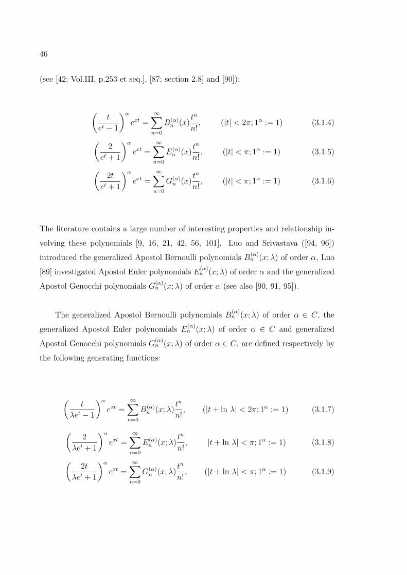
46

(see [42; Vol.III, p.253 et seq.], [87; section 2.8] and [90]):

(t

et − 1

)αext =

∞∑n=0

B(α)n (x)

tn

n!, (|t| < 2π; 1α := 1) (3.1.4)

(2

et + 1

)αext =

∞∑n=0

E(α)n (x)

tn

n!, (|t| < π; 1α := 1) (3.1.5)

(2t

et + 1

)αext =

∞∑n=0

G(α)n (x)

tn

n!, (|t| < π; 1α := 1) (3.1.6)

The literature contains a large number of interesting properties and relationship in-

volving these polynomials [9, 16, 21, 42, 56, 101]. Luo and Srivastava ([94, 96])

introduced the generalized Apostol Bernoulli polynomials B(α)n (x;λ) of order α, Luo

[89] investigated Apostol Euler polynomials E(α)n (x;λ) of order α and the generalized

Apostol Genocchi polynomials G(α)n (x;λ) of order α (see also [90, 91, 95]).

The generalized Apostol Bernoulli polynomials B(α)n (x;λ) of order α ∈ C, the

generalized Apostol Euler polynomials E(α)n (x;λ) of order α ∈ C and generalized

Apostol Genocchi polynomials G(α)n (x;λ) of order α ∈ C, are defined respectively by

the following generating functions:

(t

λet − 1

)αext =

∞∑n=0

B(α)n (x;λ)

tn

n!, (|t+ ln λ| < 2π; 1α := 1) (3.1.7)

(2

λet + 1

)αext =

∞∑n=0

E(α)n (x;λ)

tn

n!, |t+ ln λ| < π; 1α := 1) (3.1.8)

(2t

λet + 1

)αext =

∞∑n=0

G(α)n (x;λ)

tn

n!, (|t+ ln λ| < π; 1α := 1) (3.1.9)

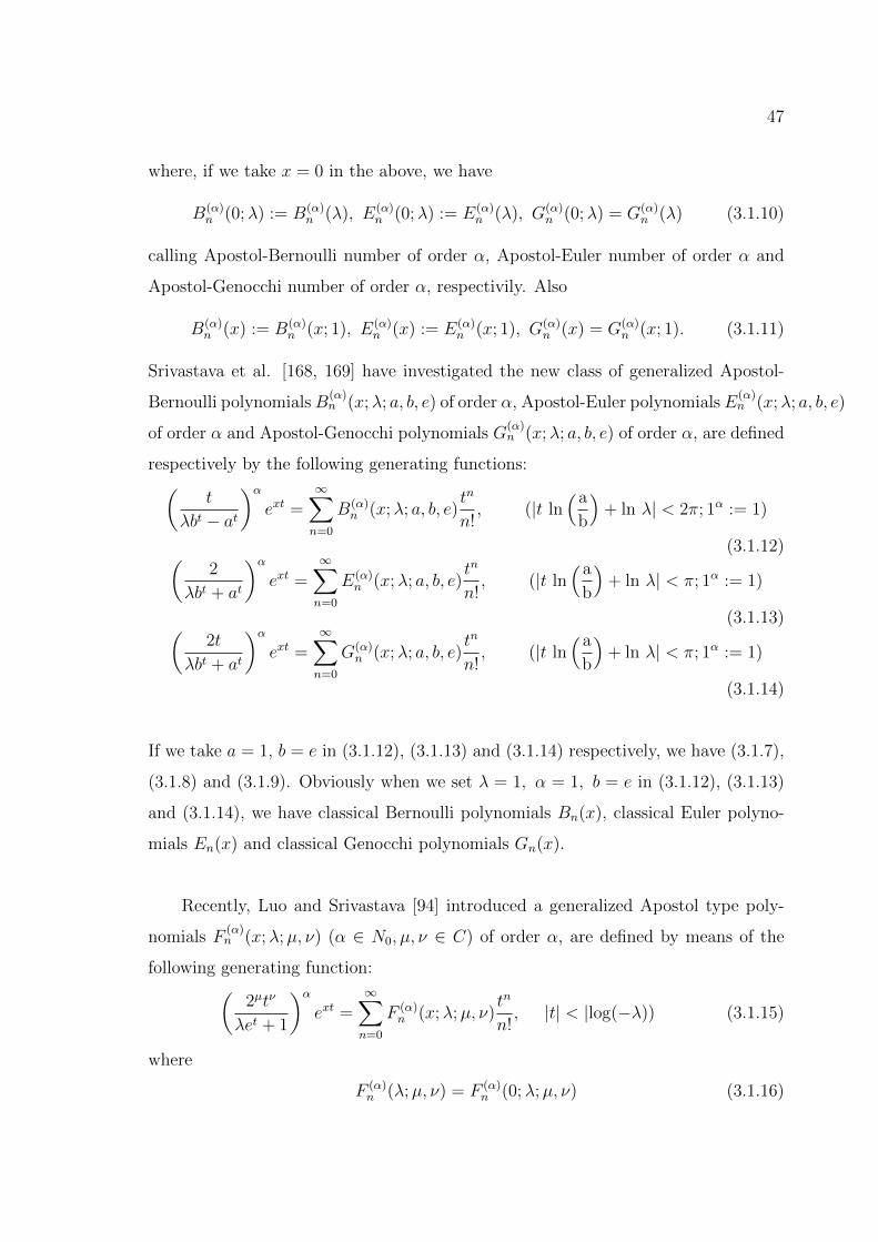
47

where, if we take x = 0 in the above, we have

B(α)n (0;λ) := B(α)

n (λ), E(α)n (0;λ) := E(α)

n (λ), G(α)n (0;λ) = G(α)

n (λ) (3.1.10)

calling Apostol-Bernoulli number of order α, Apostol-Euler number of order α and

Apostol-Genocchi number of order α, respectivily. Also

B(α)n (x) := B(α)

n (x; 1), E(α)n (x) := E(α)

n (x; 1), G(α)n (x) = G(α)

n (x; 1). (3.1.11)

Srivastava et al. [168, 169] have investigated the new class of generalized Apostol-

Bernoulli polynomialsB(α)n (x;λ; a, b, e) of order α, Apostol-Euler polynomials E

(α)n (x;λ; a, b, e)

of order α and Apostol-Genocchi polynomials G(α)n (x;λ; a, b, e) of order α, are defined

respectively by the following generating functions:(t

λbt − at

)αext =

∞∑n=0

B(α)n (x;λ; a, b, e)

tn

n!, (|t ln

(a

b

)+ ln λ| < 2π; 1α := 1)

(3.1.12)(2

λbt + at

)αext =

∞∑n=0

E(α)n (x;λ; a, b, e)

tn

n!, (|t ln

(a

b

)+ ln λ| < π; 1α := 1)

(3.1.13)(2t

λbt + at

)αext =

∞∑n=0

G(α)n (x;λ; a, b, e)

tn

n!, (|t ln

(a

b

)+ ln λ| < π; 1α := 1)

(3.1.14)

If we take a = 1, b = e in (3.1.12), (3.1.13) and (3.1.14) respectively, we have (3.1.7),

(3.1.8) and (3.1.9). Obviously when we set λ = 1, α = 1, b = e in (3.1.12), (3.1.13)

and (3.1.14), we have classical Bernoulli polynomials Bn(x), classical Euler polyno-

mials En(x) and classical Genocchi polynomials Gn(x).

Recently, Luo and Srivastava [94] introduced a generalized Apostol type poly-

nomials F(α)n (x;λ;µ, ν) (α ∈ N0, µ, ν ∈ C) of order α, are defined by means of the

following generating function:(2µtν

λet + 1

)αext =

∞∑n=0

F (α)n (x;λ;µ, ν)

tn

n!, |t| < |log(−λ)) (3.1.15)

where

F (α)n (λ;µ, ν) = F (α)

n (0;λ;µ, ν) (3.1.16)

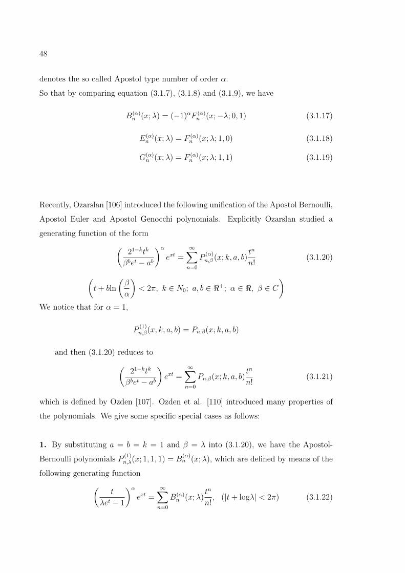
48

denotes the so called Apostol type number of order α.

So that by comparing equation (3.1.7), (3.1.8) and (3.1.9), we have

B(α)n (x;λ) = (−1)αF (α)

n (x;−λ; 0, 1) (3.1.17)

E(α)n (x;λ) = F (α)

n (x;λ; 1, 0) (3.1.18)

G(α)n (x;λ) = F (α)

n (x;λ; 1, 1) (3.1.19)

Recently, Ozarslan [106] introduced the following unification of the Apostol Bernoulli,

Apostol Euler and Apostol Genocchi polynomials. Explicitly Ozarslan studied a

generating function of the form(21−ktk

βbet − ab

)αext =

∞∑n=0

P(α)n,β (x; k, a, b)

tn

n!(3.1.20)

(t+ bln

(β

α

)< 2π, k ∈ N0; a, b ∈ <+; α ∈ <, β ∈ C

)We notice that for α = 1,

P(1)n,β(x; k, a, b) = Pn,β(x; k, a, b)

and then (3.1.20) reduces to(21−ktk

βbet − ab

)ext =

∞∑n=0

Pn,β(x; k, a, b)tn

n!(3.1.21)

which is defined by Ozden [107]. Ozden et al. [110] introduced many properties of

the polynomials. We give some specific special cases as follows:

1. By substituting a = b = k = 1 and β = λ into (3.1.20), we have the Apostol-

Bernoulli polynomials P(1)n,λ(x; 1, 1, 1) = B

(α)n (x;λ), which are defined by means of the

following generating function(t

λet − 1

)αext =

∞∑n=0

B(α)n (x;λ)

tn

n!, (|t+ logλ| < 2π) (3.1.22)

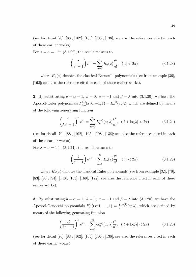
49

(see for detail [70], [88], [102], [105], [108], [138]; see also the references cited in each

of these earlier works)

For λ = α = 1 in (3.1.22), the result reduces to(t

et − 1

)ext =

∞∑n=0

Bn(x)tn

n!, (|t| < 2π) (3.1.23)

where Bn(x) denotes the classical Bernoulli polynomials (see from example [36],

[162]; see also the reference cited in each of these earlier works).

2. By substituting b = α = 1, k = 0, a = −1 and β = λ into (3.1.20), we have the

Apostol-Euler polynomials P(1)n,λ(x; 0,−1, 1) = E

(1)n (x;λ), which are defined by means

of the following generating function(2

λet + 1

)αext =

∞∑n=0

E(α)n (x;λ)

tn

n!, (|t+ logλ| < 2π) (3.1.24)

(see for detail [70], [88], [102], [105], [108], [138]; see also the references cited in each

of these earlier works)

For λ = α = 1 in (3.1.24), the result reduces to(2

et + 1

)ext =

∞∑n=0

En(x)tn

n!, (|t| < 2π) (3.1.25)

where En(x) denotes the classical Euler polynomials (see from example [32], [70],

[83], [88], [94], [140], [163], [169], [172]; see also the reference cited in each of these

earlier works).

3. By substituting b = α = 1, k = 1, a = −1 and β = λ into (3.1.20), we have the

Apostol-Genocchi polynomials P(1)n,λ(x; 1,−1, 1) = 1

2G

(1)n (x;λ), which are defined by

means of the following generating function(2t

λet + 1

)αext =

∞∑n=0

G(α)n (x;λ)

tn

n!, (|t+ logλ| < 2π) (3.1.26)

(see for detail [70], [88], [102], [105], [108], [138]; see also the references cited in each

of these earlier works)

50

For λ = α = 1 in (3.1.26), the result reduces to(2t

et + 1

)ext =

∞∑n=0

Gn(x)tn

n!, (|t| < 2π) (3.1.27)

where Gn(x) denotes the classical Genocchi polynomials (see from example [32],

[70], [83], [88], [94], [140], [163], [169], [172]; see also the reference cited in each of

these earlier works).

4. By substituting x = 0 in the generating function (3.1.20), we obtain the cor-

responding unification of the generating function of Bernoulli, Euler and Genocchi

numbers of higher order. Thus we have

P(α)n,β (0; k, a, b) = P

(α)n,β (k, a, b), n ∈ N

The 2-variable Kampe′ de Fe′riet generalization of the Hermite polynomials [14] and

[36] reads

Hn(x, y) = n!

[n2

]∑r=0

yrxn−2r

r!(n− 2r)!(3.1.28)

These polynomials are usually defined by the generating function

ext+yt2

=∞∑n=0

Hn(x, y)tn

n!(3.1.29)

and reduce to the ordinary Hermite polynomials Hn(x) (see [5]) when y = −1 and x

is replaced by 2x.

In the present chapter, we have first given the definition of the generalized

Apostol type Laguerre-Based polynomials-I LF(α)n (x, y, z;λ;µ, ν) which generalizes

the concept stated above and then find their basic properties and relationships with

Apostol type Hermite-Based polynomials HF(α)n (x, y;λ;µ, ν) of Lu et al. [93] in sec-

tion 3.2. In section 3.3 and 3.4, we have derived some implicit summation formu-

lae and general symmetry identities of the generalized Apostol type Laguerre-Based

51

polynomials LF(α)n (x, y, z;λ;µ, ν). In section 3.5, we have given the definition of

the Laguerre-based Apostol polynomials-II LP(α)n,β (x, y, z; k, a, b) which generalizes the

concept stated above and then investigate their basic properties and relationship

with Bernoulli number Bn(k, a, b), Bernoulli polynomials Bn(x; k, a, b), Euler num-

ber En(k, a, b), Euler polynomials En(x; k, a, b), Genocchi number Gn(k; a, b) and the

Genocchi polynomials Gn(x; k, a, b). Some implicit summation formulae and general

symmetry identities of the Laguerre-based Apostol Bernoulli, Euler and Genocchi

polynomials LP(α)n,β (x, y, z; k, a, b) are derived in section 3.6 and section 3.7.

3.2 Definition and Properties of the Generalized

Apostol type Laguerre-Based Polynomials-I

In this section, we have presented further definition and properties for the generalized

Apostol type Laguerre-Based polynomials LF(α)n (x, y, z;λ;µ, ν).

Definition 3.2.1. The generalized Apostol type Laguerre-Based polynomials

LF(α)n (x, y, z;λ;µ, ν) (α ∈ N0, µ, ν ∈ C) for nonnegative integer n, are defined by

∞∑n=0

LF(α)n (x, y, z;λ;µ, ν)

tn

n!=

(2µtν

λet + 1

)αeyt+zt

2

C0(xt), (|t| < |log(−λ)) (3.2.1)

so that

LF(α)n (x, y, z;λ;µ, ν) =

n∑m=0

[m2

]∑k=0

F(α)n−m(λ;µ, ν) Lm−2k(x, y)zkn!

(m− 2k)!k!(n−m)!(3.2.2)

For α = 1, in (3.2.1) we obtain the following generating function

∞∑n=0

LFn(x, y, z;λ;µ, ν)tn

n!=

(2µtν

λet + 1

)eyt+zt

2

C0(xt), (|t| < |log(−λ)) (3.2.3)

For x = 0 in (3.2.1), the result reduces to Hermite-Based generalized Apostol type

polynomials of Lu et al. [93] is defined as

∞∑n=0

HF(α)n (y, z;λ;µ, ν)

tn

n!=

(2µtν

λet + 1

)αeyt+zt

2

, (|t| < |log(−λ)) (3.2.4)

52

As in the case y = z = 0 in (3.2.1), it leads to an extension of the generalized

Apostol type polynomials denoted by F(α)n (x;λ;µ, ν) for a nonnegative integer n de-

fined earlier by (3.1.15).

The generalized Apostol type Laguerre-Based polynomials LF(α)n (x, y, z;λ;µ, ν, e)

defined by (3.2.1) have the following properties which are stated as theorem below.

Theorem 3.2.1. For any integral n ≥ 1, x, y, z ∈ R, λ ∈ C and α ∈ N .

The following relation for the generalized Apostol type Laguerre-Based polynomi-

als LF(α)n (x, y, z;λ;µ, ν) holds true:

LF(α)n (x, y, z;λ;µ, ν, e) = LF

(α)n (x, y, z;λ;µ, ν), (−1)αLF

(α)n (x, y, z;−λ; 0, 1) = LB

(α)n (x, y, z;λ)

LF(α)n (x, y, z;λ; 1, 0) = LE

(α)n (x, y, z;λ), LF

(α)n (x, y, z;λ; 1, 1) = LG

(α)n (x, y, z;λ)

(3.2.5)

LF(α+β)n (x, y + z, v + u;λ;µ, ν) =

n∑k=0

(nk

)LF

(α)n−k(x, z, v;λ;µ, ν)HF

(β)k (y, u;λ;µ, ν)

(3.2.6)

LF(α+β)n (x, y + v, z;λ;µ, ν) =

n∑k=0

(nk

)LF

(α)n−k(x, y, z;λ;µ, ν)F

(β)k (v;λ;µ, ν) (3.2.7)

Proof: The proof of (3.2.5) are obvious. Applying definition (3.2.1), we have

∞∑n=0

LF(α+β)n (x, y + z, v + u;λ;µ, ν)

tn

n!

=

(∞∑n=0

LF(α)n (x, z, v;λ;µ, ν)

tn

n!

)(∞∑k=0

HF(β)k (y, u;λ;µ, ν)

tk

k!

)

=∞∑n=0

(n∑k=0

(nk

)LF

(α)n−k(x, z, v;λ;µ, ν)HF

(β)k (x, y, u;λ;µ, ν)

)tn

n!

Now equating the coefficients of tn

n!in the above equation, we get the result (3.2.6).

Again by definition (3.2.1) of Apostol type Laguerre-Based polynomials, we have

∞∑n=0

LF(α+β)n (x, y + v, z;λ;µ, ν)

tn

n!=

(2µtν

λet + 1

)α+β

e(y+v)t+zt2C0(xt)

53

=

((2µtν

λet + 1

)αeyt+zt

2

C0(xt)

)((2µtν

λet + 1

)βevt

)which can be written as

=∞∑n=0

LF(α)n (x, y, z;λ;µ, ν)

tn

n!

∞∑k=0

F(β)k (v;λ;µ, ν)

tk

k!

=∞∑n=0

(n∑k=0

(nk

)LF

(α)n−k(x, y, z;λ;µ, ν)F

(β)k (v;λ;µ, ν)

)tn

n!

Now equating the coefficients of the like power of tn

n!in the above equation, we get

the result (3.2.7).

3.3 Implicit Summation Formulae Involving Apos-

tol type Laguerre-Based Polynomials-I

For the derivation of implicit formulae involving generalized Apostol type Laguerre-

Based polynomials LF(α)n (x, y, z;λ;µ, ν) the same consideration as developed for the

ordinary Hermite and related polynomials in Khan et al. [84] and Hermite-Bernoulli

polynomials in Pathan [118], Pathan and Khan [121] holds as well. First we prove

the following results involving generalized Apostol type Laguerre-Based polynomials

LF(α)n (x, y, z;λ;µ, ν).

Theorem 3.3.1. For any integral n ≥ 1, x, y, z ∈ R, λ ∈ C and α ∈ N . The fol-

lowing implicit summation formulae for the generalized Apostol type Laguerre-Based

polynomials LF(α)n (x, y, z;λ;µ, ν) holds true:

LF(α)m+n(x, v, z;λ;µ, ν) =

m,n∑s,k=0

(ms

)(nk

)(v − y)s+kLF

(α)m+n−s−k(x, v, z;λ;µ, ν)

(3.3.1)

Proof: We replace t by t+ u and rewrite the generating function (3.2.1) as(2µ(t+ u)ν

λet+u + 1

)αez(t+u)2C0(x(t+ u)) = e−y(t+u)

∞∑m,n=0

FG(α)m+n(x, y, z;λ;µ, ν)

tn

n!

um

m!

(3.3.2)

54

Replacing y by v in the above equation and equating the resulting equation to the

above equation, we get

e(v−y)(t+u)

∞∑m,n=0

LF(α)m+n(x, y, z;λ;µ, ν)

tn

n!

um

m!=

∞∑m,n=0

LF(α)m+n(x, v, z;λ;µ, ν)

tn

n!

um

m!

(3.3.3)

On expanding exponential function (3.3.3) gives

∞∑N=0

[(v − y)(t+ u)]N

N !

∞∑m,n=0

LF(α)m+n(x, y, z;λ;µ, ν)

tn

n!

um

m!=

∞∑m,n=0

LF(α)m+n(x, v, z;λ;µ, ν)

tn

n!

um

m!

(3.3.4)

which on using the following formula [150; p.52 (2)]

∞∑N=0

f(N)(x+ y)N

N !=

∞∑n,m=0

f(m+ n)xn

n!

ym

m!(3.3.5)

in the left hand side becomes

∞∑k,s=0

(v − y)k+s tkus

k!s!

∞∑m,n=0

LF(α)m+n(x, y, z;λ;µ, ν)

tn

n!

um

m!=

∞∑m,n=0

LF(α)m+n(x, v, z;λ;µ, ν)

tn

n!

um

m!

(3.3.6)

Now replacing n by n− k, s by n− s and using the lemma [150; p.100 (1)] in the left

hand side of (3.3.6), we get

∞∑m,n=0

∞∑k,s=0

(v − y)k+s

k!s!LF

(α)m+n−k−s(x, y, z;λ;µ, ν)

tn

(n− k)!

um

(m− s)!

=∞∑

m,n=0

LF(α)m+n(x, v, z;λ;µ, ν)

tn

n!

um

m!(3.3.7)

Finally, on equating the coefficients of the like powers of tn and um in the above

equation, we get the required result.

Remark 3.3.1. Replacing λ = −λ, µ = 0 and ν = 1 in Theorem (3.3.1) and then

multiplying (−1)α on both side of the result, we immediately deduce the following

corollary.

55

Corollary 3.3.1. The following implicit summation formula for the generalized

Apostol type Laguerre-Bernoulli polynomials LB(α)n (x, y, z;λ) holds true:

LB(α)m+n(x, v, z;λ) =

m,n∑s,k=0

(ms

)(nk

)(v − y)s+kLB

(α)m+n−s−k(x, v, z;λ) (3.3.8)

Remark 3.3.2. By taking µ = 1 and ν = 0 in Theorem (3.3.1), we immediately

deduce the following corollary.

Corollary 3.3.2. The following implicit summation formula for the generalized

Apostol type Laguerre-Euler polynomials LE(α)n (x, y, z;λ) holds true:

LE(α)m+n(x, v, z;λ) =

m,n∑s,k=0

(ms

)(nk

)(v − y)s+kLE

(α)m+n−s−k(x, v, z;λ) (3.3.9)

Remark 3.3.3. By taking µ = 1 and ν = 1 in Theorem (3.3.1), we immediately

deduce the following corollary.

Corollary 3.3.3. The following implicit summation formula for the generalized

Apostol type Laguerre-Genocchi polynomials LG(α)n (x, y, z;λ) holds true:

LG(α)m+n(x, v, z;λ) =

m,n∑s,k=0

(ms

)(nk

)(v − y)s+kLG

(α)m+n−s−k(x, v, z;λ) (3.3.10)

Theorem 3.3.2. For any integral n ≥ 1, x, y, z ∈ R, λ ∈ C and α ∈ N . The fol-

lowing implicit summation formula for the generalized Apostol type Laguerre-Based

polynomials LF(α)n (x, y, z;λ;µ, ν) holds true:

LF(α)n (x, y + u, z;λ;µ, ν) =

n∑j=0

(nj

)ujLF

(α)n−j(x, y, z;λ;µ, ν) (3.3.11)

Proof: Since

∞∑n=0

LF(α)n (x, y + u, z;λ;µ, ν)

tn

n!=

(2µtν

λet + 1

)αe(y+u)t+zt2C0(xt)

56

∞∑n=0

LF(α)n (x, y + u, z;λ;µ, ν)

tn

n!=

(∞∑n=0

LF(α)n (x, y, z;λ;µ, ν)

tn

n!

)(∞∑j=0

ujtj

j!

)Now, replacing n by n − j and comparing the coefficients of tn, we get the result

(3.3.11).

Remark 3.3.4. Replacing λ = −λ, µ = 0 and ν = 1 in Theorem (3.3.2) and then

multiplying (−1)α on both side of the result, we immediately deduce the following

corollary.

Corollary 3.3.4. The following implicit summation formula for the generalized

Apostol type Laguerre-Bernoulli polynomials LB(α)n (x, y, z;λ) holds true:

LB(α)n (x, y + u, z;λ) =

n∑j=0

(nj

)ujLB

(α)n−j(x, y, z;λ) (3.3.12)

Remark 3.3.5. By taking µ = 1 and ν = 0 in Theorem (3.3.2), we immediately

deduce the following corollary.

Corollary 3.3.5. The following implicit summation formula for the generalized

Apostol type Laguerre-Euler polynomials LE(α)n (x, y, z;λ) holds true:

LE(α)n (x, y + u, z;λ) =

n∑j=0

(nj

)ujLE

(α)n−j(x, y, z;λ) (3.3.13)

Remark 3.3.6. By taking µ = 1 and ν = 1 in Theorem (3.3.2), we immediately

deduce the following corollary.

Corollary 3.3.6. The following implicit summation formula for the generalized

Apostol type Laguerre-Genocchi polynomials LG(α)n (x, y, z;λ) holds true:

LG(α)n (x, y + u, z;λ) =

n∑j=0

(nj

)ujLG

(α)n−j(x, y, z;λ) (3.3.14)

57

Theorem 3.3.3. For any integral n ≥ 1, x, y, z ∈ R, λ ∈ C and α ∈ N . The fol-

lowing implicit summation formula for the generalized Apostol type Laguerre-Based

polynomials LF(α)n (x, y, z;λ;µ, ν) holds true:

LF(α)n (x, y + u, z + w;λ;µ, ν) =

n∑m=0

(nm

)LF

(α)n−m(x, y, z;λ;µ, ν)Hm(u,w) (3.3.15)

Proof: By the definition of Apostol type Laguerre-Based polynomials and the defi-

nition (3.1.29), we have(2µtν

λet + 1

)αe(y+u)t+(z+w)t2C0(xt) =

(∞∑n=0

LG(k)n (x, y, z)

tn

n!

)(∞∑m=0

Hm(u,w)tm

m!

)Now, replacing n by n − m and comparing the coefficients of tn, we get the result

(3.3.15).

Remark 3.3.7. Replacing λ = −λ, µ = 0 and ν = 1 in Theorem (3.3.3) and then

multiplying (−1)α on both side of the result, we immediately deduce the following

corollary.

Corollary 3.3.7. The following implicit summation formula for the generalized

Apostol type Laguerre-Bernoulli polynomials LB(α)n (x, y, z;λ) holds true:

LB(α)n (x, y + u, z + w;λ) =

n∑m=0

(nm

)LB

(α)n−m(x, y, z;λ)Hm(u,w) (3.3.16)

Remark 3.3.8. By taking µ = 1 and ν = 0 in Theorem (3.3.3), we immediately

deduce the following corollary.

Corollary 3.3.8. The following implicit summation formula for the generalized

Apostol type Laguerre-Euler polynomials LE(α)n (x, y, z;λ) holds true:

LE(α)n (x, y + u, z + w;λ) =

n∑m=0

(nm

)LE

(α)n−m(x, y, z;λ)Hm(u,w) (3.3.17)

Remark 3.3.9. By taking µ = 1 and ν = 1 in Theorem (3.3.3), we immediately

deduce the following corollary.

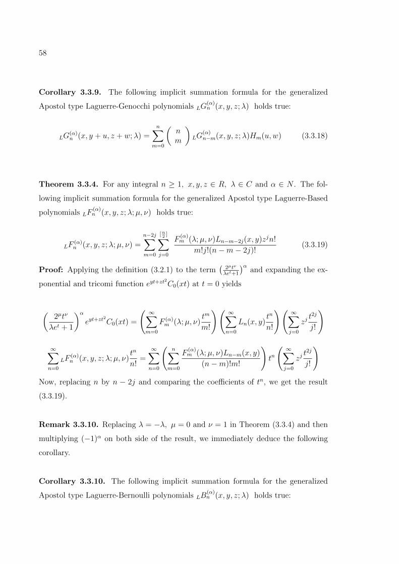
58

Corollary 3.3.9. The following implicit summation formula for the generalized

Apostol type Laguerre-Genocchi polynomials LG(α)n (x, y, z;λ) holds true:

LG(α)n (x, y + u, z + w;λ) =

n∑m=0

(nm

)LG

(α)n−m(x, y, z;λ)Hm(u,w) (3.3.18)

Theorem 3.3.4. For any integral n ≥ 1, x, y, z ∈ R, λ ∈ C and α ∈ N . The fol-

lowing implicit summation formula for the generalized Apostol type Laguerre-Based

polynomials LF(α)n (x, y, z;λ;µ, ν) holds true:

LF(α)n (x, y, z;λ;µ, ν) =

n−2j∑m=0

[n2

]∑j=0

F(α)m (λ;µ, ν)Ln−m−2j(x, y)zjn!

m!j!(n−m− 2j)!(3.3.19)

Proof: Applying the definition (3.2.1) to the term(

2µtν

λet+1

)αand expanding the ex-

ponential and tricomi function eyt+zt2C0(xt) at t = 0 yields

(2µtν

λet + 1

)αeyt+zt

2

C0(xt) =

(∞∑m=0

F (α)m (λ;µ, ν)

tm

m!

)(∞∑n=0

Ln(x, y)tn

n!

)(∞∑j=0

zjt2j

j!

)

∞∑n=0

LF(α)n (x, y, z;λ;µ, ν)

tn

n!=∞∑n=0

(n∑

m=0

F(α)m (λ;µ, ν)Ln−m(x, y)

(n−m)!m!

)tn

(∞∑j=0

zjt2j

j!

)

Now, replacing n by n − 2j and comparing the coefficients of tn, we get the result

(3.3.19).

Remark 3.3.10. Replacing λ = −λ, µ = 0 and ν = 1 in Theorem (3.3.4) and then

multiplying (−1)α on both side of the result, we immediately deduce the following

corollary.

Corollary 3.3.10. The following implicit summation formula for the generalized

Apostol type Laguerre-Bernoulli polynomials LB(α)n (x, y, z;λ) holds true:

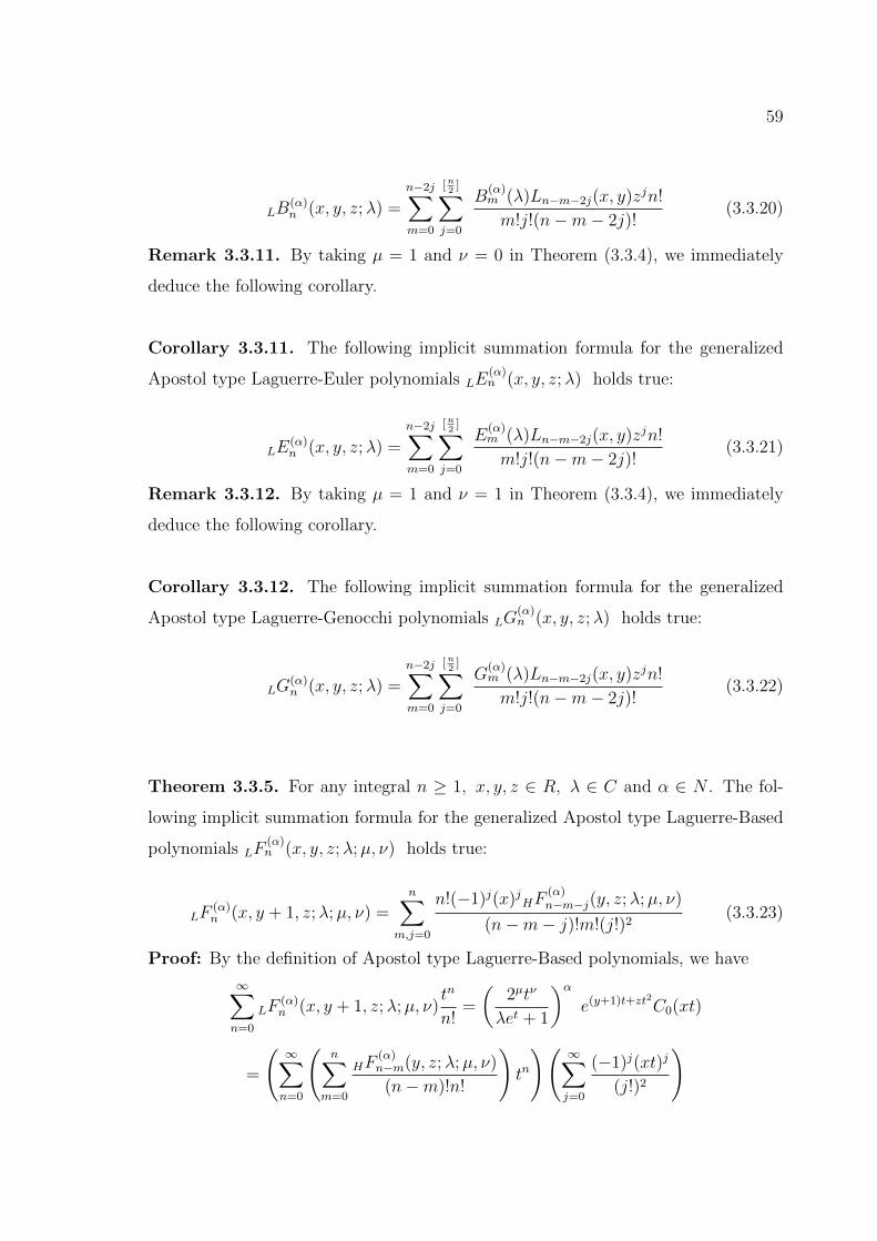
59

LB(α)n (x, y, z;λ) =

n−2j∑m=0

[n2

]∑j=0

B(α)m (λ)Ln−m−2j(x, y)zjn!

m!j!(n−m− 2j)!(3.3.20)

Remark 3.3.11. By taking µ = 1 and ν = 0 in Theorem (3.3.4), we immediately

deduce the following corollary.

Corollary 3.3.11. The following implicit summation formula for the generalized

Apostol type Laguerre-Euler polynomials LE(α)n (x, y, z;λ) holds true:

LE(α)n (x, y, z;λ) =

n−2j∑m=0

[n2

]∑j=0

E(α)m (λ)Ln−m−2j(x, y)zjn!

m!j!(n−m− 2j)!(3.3.21)

Remark 3.3.12. By taking µ = 1 and ν = 1 in Theorem (3.3.4), we immediately

deduce the following corollary.

Corollary 3.3.12. The following implicit summation formula for the generalized

Apostol type Laguerre-Genocchi polynomials LG(α)n (x, y, z;λ) holds true:

LG(α)n (x, y, z;λ) =

n−2j∑m=0

[n2

]∑j=0

G(α)m (λ)Ln−m−2j(x, y)zjn!

m!j!(n−m− 2j)!(3.3.22)

Theorem 3.3.5. For any integral n ≥ 1, x, y, z ∈ R, λ ∈ C and α ∈ N . The fol-

lowing implicit summation formula for the generalized Apostol type Laguerre-Based

polynomials LF(α)n (x, y, z;λ;µ, ν) holds true:

LF(α)n (x, y + 1, z;λ;µ, ν) =

n∑m,j=0

n!(−1)j(x)jHF(α)n−m−j(y, z;λ;µ, ν)

(n−m− j)!m!(j!)2(3.3.23)

Proof: By the definition of Apostol type Laguerre-Based polynomials, we have

∞∑n=0

LF(α)n (x, y + 1, z;λ;µ, ν)

tn

n!=

(2µtν

λet + 1

)αe(y+1)t+zt2C0(xt)

=

(∞∑n=0

(n∑

m=0

HF(α)n−m(y, z;λ;µ, ν)

(n−m)!n!

)tn

)(∞∑j=0

(−1)j(xt)j

(j!)2

)

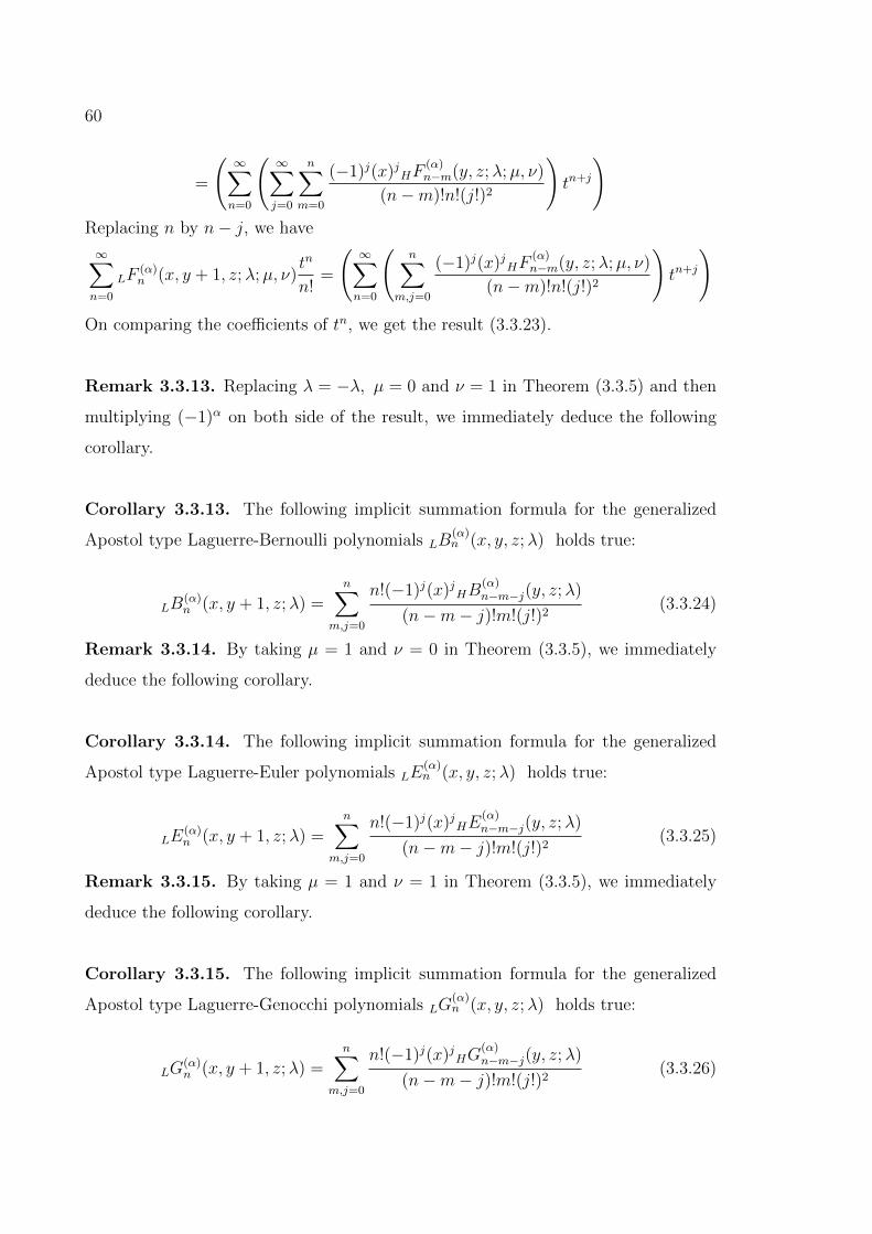
60

=

(∞∑n=0

(∞∑j=0

n∑m=0

(−1)j(x)jHF(α)n−m(y, z;λ;µ, ν)

(n−m)!n!(j!)2

)tn+j

)Replacing n by n− j, we have

∞∑n=0

LF(α)n (x, y + 1, z;λ;µ, ν)

tn

n!=

(∞∑n=0

(n∑

m,j=0

(−1)j(x)jHF(α)n−m(y, z;λ;µ, ν)

(n−m)!n!(j!)2

)tn+j

)On comparing the coefficients of tn, we get the result (3.3.23).

Remark 3.3.13. Replacing λ = −λ, µ = 0 and ν = 1 in Theorem (3.3.5) and then

multiplying (−1)α on both side of the result, we immediately deduce the following

corollary.

Corollary 3.3.13. The following implicit summation formula for the generalized

Apostol type Laguerre-Bernoulli polynomials LB(α)n (x, y, z;λ) holds true:

LB(α)n (x, y + 1, z;λ) =

n∑m,j=0

n!(−1)j(x)jHB(α)n−m−j(y, z;λ)

(n−m− j)!m!(j!)2(3.3.24)

Remark 3.3.14. By taking µ = 1 and ν = 0 in Theorem (3.3.5), we immediately

deduce the following corollary.

Corollary 3.3.14. The following implicit summation formula for the generalized

Apostol type Laguerre-Euler polynomials LE(α)n (x, y, z;λ) holds true:

LE(α)n (x, y + 1, z;λ) =

n∑m,j=0

n!(−1)j(x)jHE(α)n−m−j(y, z;λ)

(n−m− j)!m!(j!)2(3.3.25)

Remark 3.3.15. By taking µ = 1 and ν = 1 in Theorem (3.3.5), we immediately

deduce the following corollary.

Corollary 3.3.15. The following implicit summation formula for the generalized

Apostol type Laguerre-Genocchi polynomials LG(α)n (x, y, z;λ) holds true:

LG(α)n (x, y + 1, z;λ) =

n∑m,j=0

n!(−1)j(x)jHG(α)n−m−j(y, z;λ)

(n−m− j)!m!(j!)2(3.3.26)

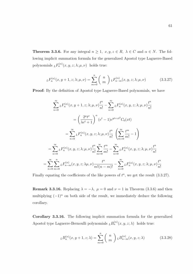
61

Theorem 3.3.6. For any integral n ≥ 1, x, y, z ∈ R, λ ∈ C and α ∈ N . The fol-

lowing implicit summation formula for the generalized Apostol type Laguerre-Based

polynomials LF(α)n (x, y, z;λ;µ, ν) holds true:

LF(α)n (x, y + 1, z;λ;µ, ν) =

n∑m=0

(nm

)LF

(α)n−m(x, y, z;λ;µ, ν) (3.3.27)

Proof: By the definition of Apostol type Laguerre-Based polynomials, we have

∞∑n=0

LF(α)n (x, y + 1, z;λ;µ, ν)

tn

n!−∞∑n=0

LF(α)n (x, y, z;λ;µ, ν)

tn

n!

=

(2µtν

λet + 1

)α(et − 1)eyt+zt

2

C0(xt)

=∞∑n=0

LF(α)n (x, y, z;λ;µ, ν)

tn

n!

(∞∑m=0

tm

m!− 1

)

=∞∑n=0

LF(α)n (x, y, z;λ;µ, ν)

tn

n!

∞∑m=0

tm

m!−∞∑n=0

LF(α)n (x, y, z;λ;µ, ν)

tn

n!

=∞∑n=0

n∑m=0

LF(α)n−m(x, y, z;λµ, ν)

tn

m!(n−m)!−∞∑n=0

LF(α)n (x, y, z;λ;µ, ν)

tn

n!

Finally equating the coefficients of the like powers of tn, we get the result (3.3.27).

Remark 3.3.16. Replacing λ = −λ, µ = 0 and ν = 1 in Theorem (3.3.6) and then

multiplying (−1)α on both side of the result, we immediately deduce the following

corollary.

Corollary 3.3.16. The following implicit summation formula for the generalized

Apostol type Laguerre-Bernoulli polynomials LB(α)n (x, y, z;λ) holds true:

LB(α)n (x, y + 1, z;λ) =

n∑m=0

(nm

)LB

(α)n−m(x, y, z;λ) (3.3.28)

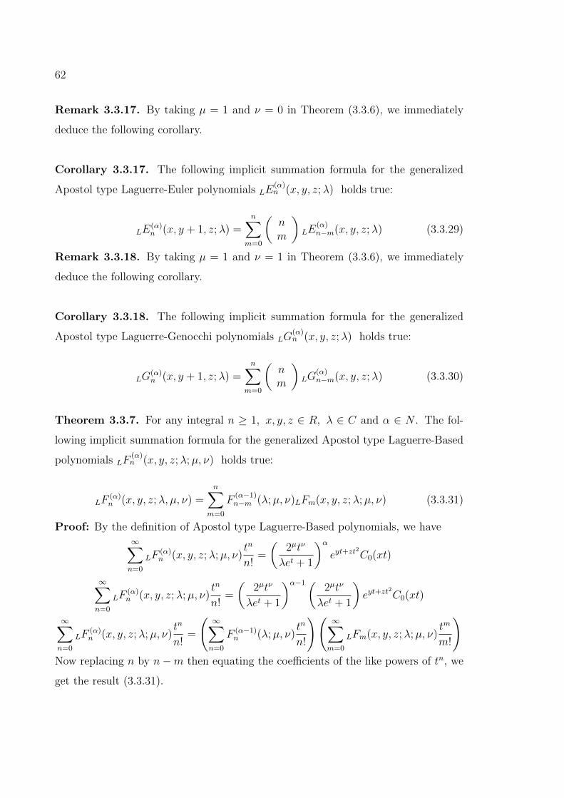
62

Remark 3.3.17. By taking µ = 1 and ν = 0 in Theorem (3.3.6), we immediately

deduce the following corollary.

Corollary 3.3.17. The following implicit summation formula for the generalized

Apostol type Laguerre-Euler polynomials LE(α)n (x, y, z;λ) holds true:

LE(α)n (x, y + 1, z;λ) =

n∑m=0

(nm

)LE

(α)n−m(x, y, z;λ) (3.3.29)

Remark 3.3.18. By taking µ = 1 and ν = 1 in Theorem (3.3.6), we immediately

deduce the following corollary.

Corollary 3.3.18. The following implicit summation formula for the generalized

Apostol type Laguerre-Genocchi polynomials LG(α)n (x, y, z;λ) holds true:

LG(α)n (x, y + 1, z;λ) =

n∑m=0

(nm

)LG

(α)n−m(x, y, z;λ) (3.3.30)

Theorem 3.3.7. For any integral n ≥ 1, x, y, z ∈ R, λ ∈ C and α ∈ N . The fol-

lowing implicit summation formula for the generalized Apostol type Laguerre-Based

polynomials LF(α)n (x, y, z;λ;µ, ν) holds true:

LF(α)n (x, y, z;λ, µ, ν) =

n∑m=0

F(α−1)n−m (λ;µ, ν)LFm(x, y, z;λ;µ, ν) (3.3.31)

Proof: By the definition of Apostol type Laguerre-Based polynomials, we have∞∑n=0

LF(α)n (x, y, z;λ;µ, ν)

tn

n!=

(2µtν

λet + 1

)αeyt+zt

2

C0(xt)

∞∑n=0

LF(α)n (x, y, z;λ;µ, ν)

tn

n!=

(2µtν

λet + 1

)α−1(2µtν

λet + 1

)eyt+zt

2

C0(xt)

∞∑n=0

LF(α)n (x, y, z;λ;µ, ν)

tn

n!=

(∞∑n=0

F (α−1)n (λ;µ, ν)

tn

n!

)(∞∑m=0

LFm(x, y, z;λ;µ, ν)tm

m!

)Now replacing n by n−m then equating the coefficients of the like powers of tn, we

get the result (3.3.31).

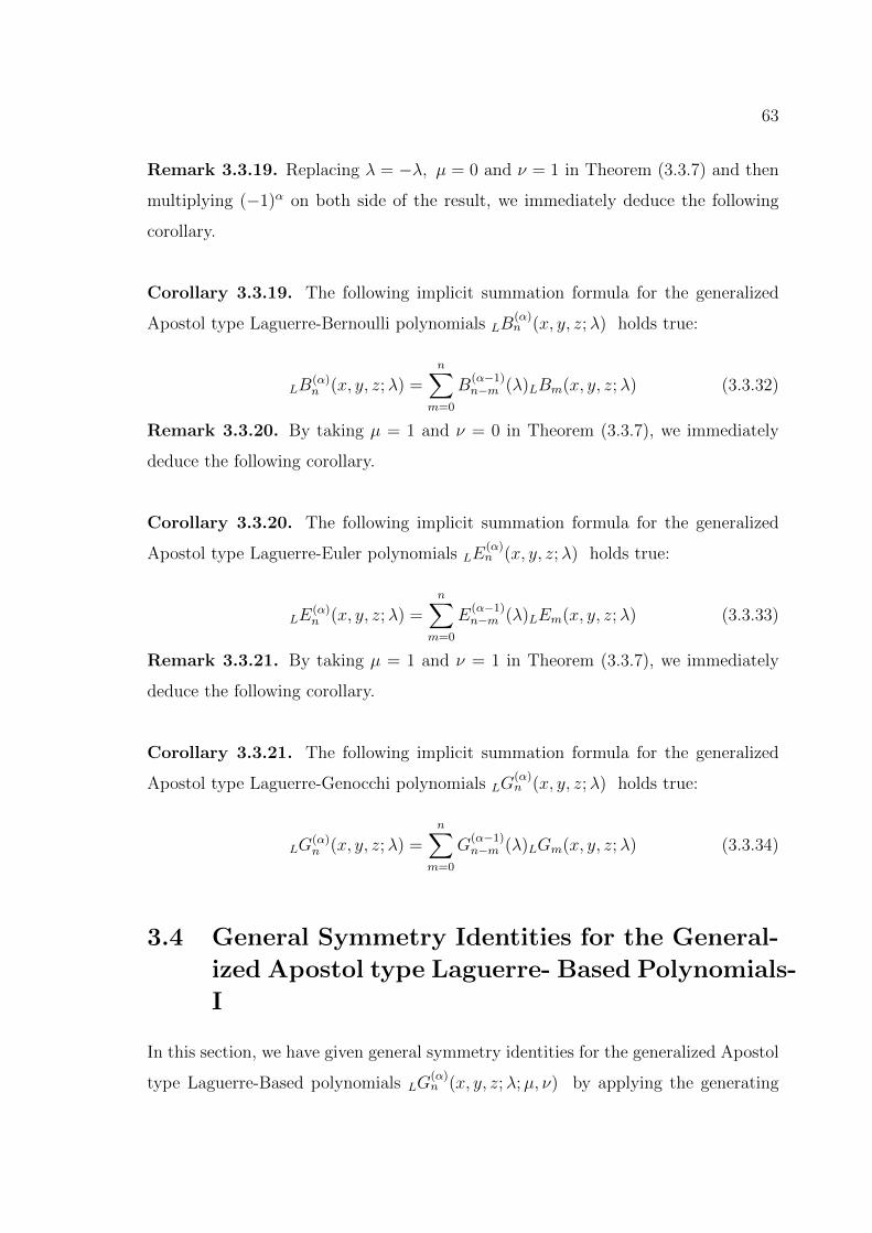
63

Remark 3.3.19. Replacing λ = −λ, µ = 0 and ν = 1 in Theorem (3.3.7) and then

multiplying (−1)α on both side of the result, we immediately deduce the following

corollary.

Corollary 3.3.19. The following implicit summation formula for the generalized

Apostol type Laguerre-Bernoulli polynomials LB(α)n (x, y, z;λ) holds true:

LB(α)n (x, y, z;λ) =

n∑m=0

B(α−1)n−m (λ)LBm(x, y, z;λ) (3.3.32)

Remark 3.3.20. By taking µ = 1 and ν = 0 in Theorem (3.3.7), we immediately

deduce the following corollary.

Corollary 3.3.20. The following implicit summation formula for the generalized

Apostol type Laguerre-Euler polynomials LE(α)n (x, y, z;λ) holds true:

LE(α)n (x, y, z;λ) =

n∑m=0

E(α−1)n−m (λ)LEm(x, y, z;λ) (3.3.33)

Remark 3.3.21. By taking µ = 1 and ν = 1 in Theorem (3.3.7), we immediately

deduce the following corollary.

Corollary 3.3.21. The following implicit summation formula for the generalized

Apostol type Laguerre-Genocchi polynomials LG(α)n (x, y, z;λ) holds true:

LG(α)n (x, y, z;λ) =

n∑m=0

G(α−1)n−m (λ)LGm(x, y, z;λ) (3.3.34)

3.4 General Symmetry Identities for the General-

ized Apostol type Laguerre- Based Polynomials-

I

In this section, we have given general symmetry identities for the generalized Apostol

type Laguerre-Based polynomials LG(α)n (x, y, z;λ;µ, ν) by applying the generating

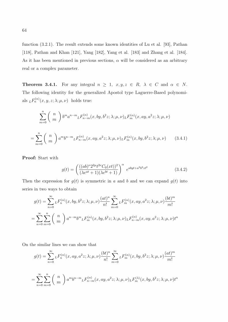
64

function (3.2.1). The result extends some known identities of Lu et al. [93], Pathan

[118], Pathan and Khan [121], Yang [182], Yang et al. [183] and Zhang et al. [184].

As it has been mentioned in previous sections, α will be considered as an arbitrary

real or a complex parameter.

Theorem 3.4.1. For any integral n ≥ 1, x, y, z ∈ R, λ ∈ C and α ∈ N .

The following identity for the generalized Apostol type Laguerre-Based polynomi-

als LF(α)n (x, y, z;λ;µ, ν) holds true:

n∑m=0

(nm

)bman−mLF

(α)n−m(x, by, b2z;λ;µ, ν)LF

(α)m (x, ay, a2z;λ;µ, ν)

=n∑

m=0

(nm

)ambn−mLF

(α)n−m(x, ay, a2z;λ;µ, ν)LF

(α)m (x, by, b2z;λ;µ, ν) (3.4.1)

Proof: Start with

g(t) =

(((ab)ν22µt2νC0(xt))2

(λeat + 1)(λebt + 1)

)αeabyt+a

2b2zt2 (3.4.2)

Then the expression for g(t) is symmetric in a and b and we can expand g(t) into

series in two ways to obtain

g(t) =∞∑n=0

LF(α)n (x, by, b2z;λ;µ, ν)

(at)n

n!

∞∑m=0

LF(α)m (x, ay, a2z;λ;µ, ν)

(bt)m

m!

=∞∑n=0

n∑m=0

(nm

)an−mbmLF

(α)m (x, by, b2z;λ;µ, ν)LF

(α)n−m(x, ay, a2z;λ;µ, ν)tn

On the similar lines we can show that

g(t) =∞∑n=0

LF(α)n (x, ay, a2z;λ;µ, ν)

(bt)n

n!

∞∑m=0

LF(α)m (x, by, b2z;λ;µ, ν)

(at)m

m!

=∞∑n=0

n∑m=0

(nm

)ambn−mLF

(α)n−m(x, ay, a2z;λ;µ, ν)LF

(λ)m (x, by, b2z;λ;µ, ν)tn

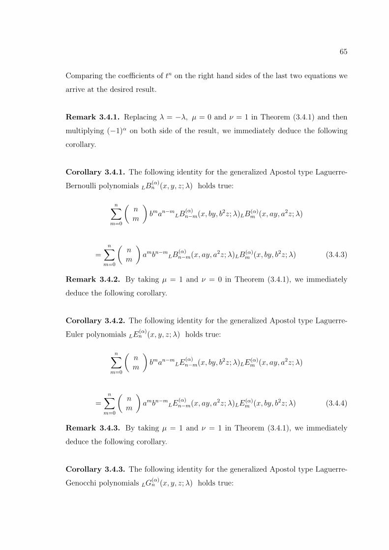
65

Comparing the coefficients of tn on the right hand sides of the last two equations we

arrive at the desired result.

Remark 3.4.1. Replacing λ = −λ, µ = 0 and ν = 1 in Theorem (3.4.1) and then

multiplying (−1)α on both side of the result, we immediately deduce the following

corollary.

Corollary 3.4.1. The following identity for the generalized Apostol type Laguerre-

Bernoulli polynomials LB(α)n (x, y, z;λ) holds true:

n∑m=0

(nm

)bman−mLB

(α)n−m(x, by, b2z;λ)LB

(α)m (x, ay, a2z;λ)

=n∑

m=0

(nm

)ambn−mLB

(α)n−m(x, ay, a2z;λ)LB

(α)m (x, by, b2z;λ) (3.4.3)

Remark 3.4.2. By taking µ = 1 and ν = 0 in Theorem (3.4.1), we immediately

deduce the following corollary.

Corollary 3.4.2. The following identity for the generalized Apostol type Laguerre-

Euler polynomials LE(α)n (x, y, z;λ) holds true:

n∑m=0

(nm

)bman−mLE

(α)n−m(x, by, b2z;λ)LE

(α)m (x, ay, a2z;λ)

=n∑

m=0

(nm

)ambn−mLE

(α)n−m(x, ay, a2z;λ)LE

(α)m (x, by, b2z;λ) (3.4.4)

Remark 3.4.3. By taking µ = 1 and ν = 1 in Theorem (3.4.1), we immediately

deduce the following corollary.

Corollary 3.4.3. The following identity for the generalized Apostol type Laguerre-

Genocchi polynomials LG(α)n (x, y, z;λ) holds true:

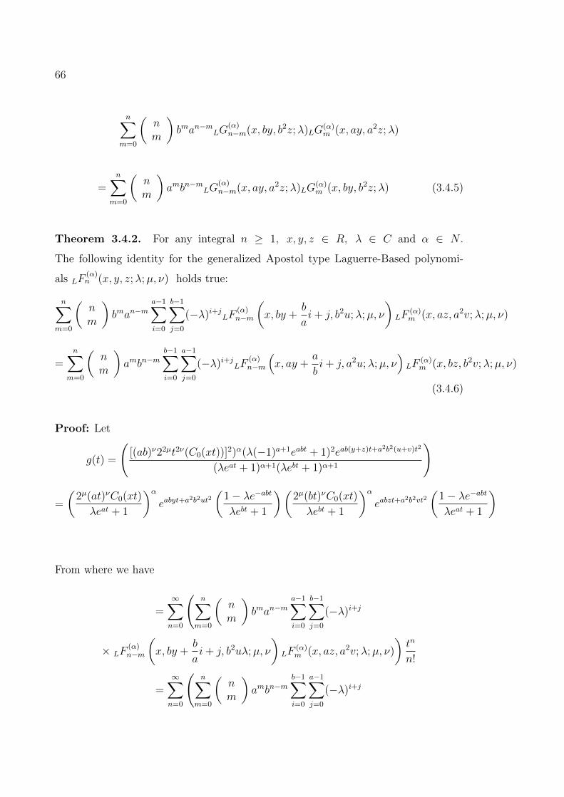
66

n∑m=0

(nm

)bman−mLG

(α)n−m(x, by, b2z;λ)LG

(α)m (x, ay, a2z;λ)

=n∑

m=0

(nm

)ambn−mLG

(α)n−m(x, ay, a2z;λ)LG

(α)m (x, by, b2z;λ) (3.4.5)

Theorem 3.4.2. For any integral n ≥ 1, x, y, z ∈ R, λ ∈ C and α ∈ N .

The following identity for the generalized Apostol type Laguerre-Based polynomi-

als LF(α)n (x, y, z;λ;µ, ν) holds true:

n∑m=0

(nm

)bman−m

a−1∑i=0

b−1∑j=0

(−λ)i+jLF(α)n−m

(x, by +

b

ai+ j, b2u;λ;µ, ν

)LF

(α)m (x, az, a2v;λ;µ, ν)

=n∑

m=0

(nm

)ambn−m

b−1∑i=0

a−1∑j=0

(−λ)i+jLF(α)n−m

(x, ay +

a

bi+ j, a2u;λ;µ, ν

)LF

(α)m (x, bz, b2v;λ;µ, ν)

(3.4.6)

Proof: Let

g(t) =

([(ab)ν22µt2ν(C0(xt))]2)α(λ(−1)a+1eabt + 1)2eab(y+z)t+a2b2(u+v)t2

(λeat + 1)α+1(λebt + 1)α+1

)

=

(2µ(at)νC0(xt)

λeat + 1

)αeabyt+a

2b2ut2(

1− λe−abt

λebt + 1

)(2µ(bt)νC0(xt)

λebt + 1

)αeabzt+a

2b2vt2(

1− λe−abt

λeat + 1

)

From where we have

=∞∑n=0

(n∑

m=0

(nm

)bman−m

a−1∑i=0

b−1∑j=0

(−λ)i+j

× LF(α)n−m

(x, by +

b

ai+ j, b2uλ;µ, ν

)LF

(α)m (x, az, a2v;λ;µ, ν)

)tn

n!

=∞∑n=0

(n∑

m=0

(nm

)ambn−m

b−1∑i=0

a−1∑j=0

(−λ)i+j

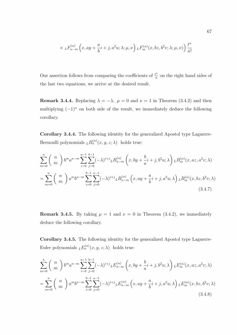
67

× LF(α)n−m

(x, ay +

a

bi+ j, a2u;λ;µ, ν

)LF

(α)m (x, bz, b2v;λ;µ, ν)

) tnn!

Our assertion follows from comparing the coefficients of tn

non the right hand sides of

the last two equations, we arrive at the desired result.

Remark 3.4.4. Replacing λ = −λ, µ = 0 and ν = 1 in Theorem (3.4.2) and then

multiplying (−1)α on both side of the result, we immediately deduce the following

corollary.

Corollary 3.4.4. The following identity for the generalized Apostol type Laguerre-

Bernoulli polynomials LB(α)n (x, y, z;λ) holds true:

n∑m=0

(nm

)bman−m

a−1∑i=0

b−1∑j=0

(−λ)i+jLB(α)n−m

(x, by +

b

ai+ j, b2u;λ

)LB

(α)m (x, az, a2v;λ)

=n∑

m=0

(nm

)ambn−m

b−1∑i=0

a−1∑j=0

(−λ)i+jLB(α)n−m

(x, ay +

a

bi+ j, a2u;λ

)LB

(α)m (x, bz, b2v;λ)

(3.4.7)

Remark 3.4.5. By taking µ = 1 and ν = 0 in Theorem (3.4.2), we immediately

deduce the following corollary.

Corollary 3.4.5. The following identity for the generalized Apostol type Laguerre-

Euler polynomials LE(α)n (x, y, z;λ) holds true:

n∑m=0

(nm

)bman−m

a−1∑i=0

b−1∑j=0

(−λ)i+jLE(α)n−m

(x, by +

b

ai+ j, b2u;λ

)LE

(α)m (x, az, a2v;λ)

=n∑

m=0

(nm

)ambn−m

b−1∑i=0

a−1∑j=0

(−λ)i+jLE(α)n−m

(x, ay +

a

bi+ j, a2u;λ

)LE

(α)m (x, bz, b2v;λ)

(3.4.8)

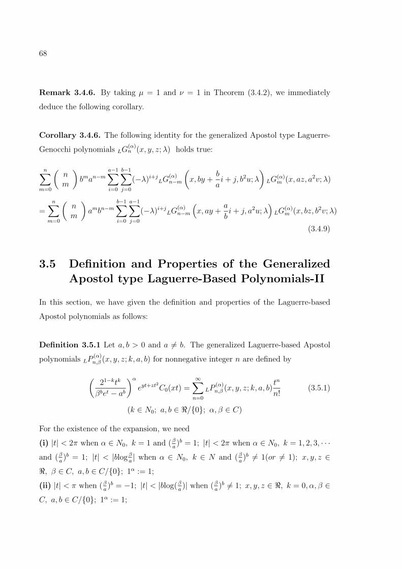
68

Remark 3.4.6. By taking µ = 1 and ν = 1 in Theorem (3.4.2), we immediately

deduce the following corollary.

Corollary 3.4.6. The following identity for the generalized Apostol type Laguerre-

Genocchi polynomials LG(α)n (x, y, z;λ) holds true:

n∑m=0

(nm

)bman−m

a−1∑i=0

b−1∑j=0

(−λ)i+jLG(α)n−m

(x, by +

b

ai+ j, b2u;λ

)LG

(α)m (x, az, a2v;λ)

=n∑

m=0

(nm

)ambn−m

b−1∑i=0

a−1∑j=0

(−λ)i+jLG(α)n−m

(x, ay +

a

bi+ j, a2u;λ

)LG

(α)m (x, bz, b2v;λ)

(3.4.9)

3.5 Definition and Properties of the Generalized

Apostol type Laguerre-Based Polynomials-II

In this section, we have given the definition and properties of the Laguerre-based

Apostol polynomials as follows:

Definition 3.5.1 Let a, b > 0 and a 6= b. The generalized Laguerre-based Apostol

polynomials LP(α)n,β (x, y, z; k, a, b) for nonnegative integer n are defined by

(21−ktk

βbet − ab

)αeyt+zt

2

C0(xt) =∞∑n=0

LP(α)n,β (x, y, z; k, a, b)

tn

n!(3.5.1)

(k ∈ N0; a, b ∈ </0; α, β ∈ C)

For the existence of the expansion, we need

(i) |t| < 2π when α ∈ N0, k = 1 and (βa)b = 1; |t| < 2π when α ∈ N0, k = 1, 2, 3, · · ·

and (βa)b = 1; |t| < |blogβ

a| when α ∈ N0, k ∈ N and (β

a)b 6= 1(or 6= 1); x, y, z ∈

<, β ∈ C, a, b ∈ C/0; 1α := 1;

(ii) |t| < π when (βa)b = −1; |t| < |blog(β

a)| when (β

a)b 6= 1; x, y, z ∈ <, k = 0, α, β ∈

C, a, b ∈ C/0; 1α := 1;

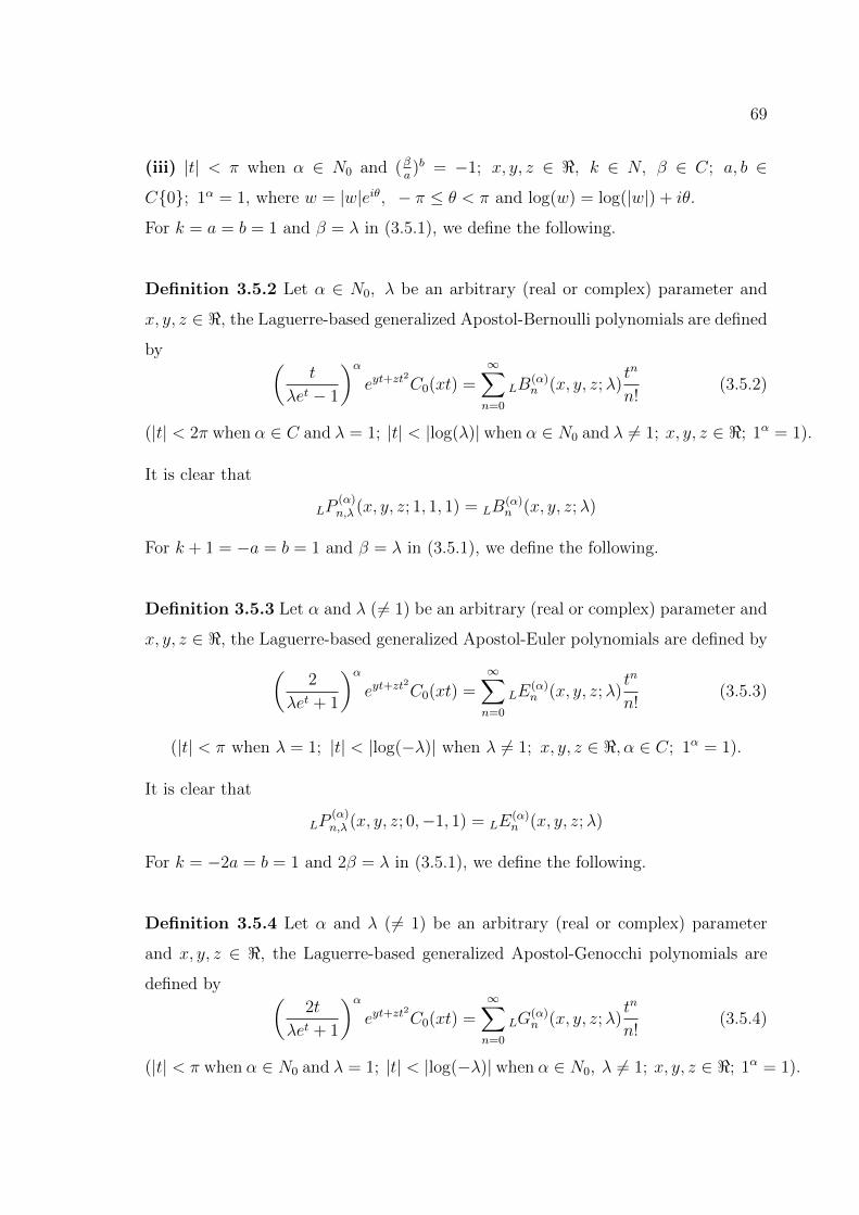
69

(iii) |t| < π when α ∈ N0 and (βa)b = −1; x, y, z ∈ <, k ∈ N, β ∈ C; a, b ∈

C0; 1α = 1, where w = |w|eiθ, − π ≤ θ < π and log(w) = log(|w|) + iθ.

For k = a = b = 1 and β = λ in (3.5.1), we define the following.

Definition 3.5.2 Let α ∈ N0, λ be an arbitrary (real or complex) parameter and

x, y, z ∈ <, the Laguerre-based generalized Apostol-Bernoulli polynomials are defined

by (t

λet − 1

)αeyt+zt

2

C0(xt) =∞∑n=0

LB(α)n (x, y, z;λ)

tn

n!(3.5.2)

(|t| < 2π when α ∈ C and λ = 1; |t| < |log(λ)| when α ∈ N0 and λ 6= 1; x, y, z ∈ <; 1α = 1).

It is clear that

LP(α)n,λ (x, y, z; 1, 1, 1) = LB

(α)n (x, y, z;λ)

For k + 1 = −a = b = 1 and β = λ in (3.5.1), we define the following.

Definition 3.5.3 Let α and λ (6= 1) be an arbitrary (real or complex) parameter and

x, y, z ∈ <, the Laguerre-based generalized Apostol-Euler polynomials are defined by(2

λet + 1

)αeyt+zt

2

C0(xt) =∞∑n=0

LE(α)n (x, y, z;λ)

tn

n!(3.5.3)

(|t| < π when λ = 1; |t| < |log(−λ)| when λ 6= 1; x, y, z ∈ <, α ∈ C; 1α = 1).

It is clear that

LP(α)n,λ (x, y, z; 0,−1, 1) = LE

(α)n (x, y, z;λ)

For k = −2a = b = 1 and 2β = λ in (3.5.1), we define the following.

Definition 3.5.4 Let α and λ (6= 1) be an arbitrary (real or complex) parameter

and x, y, z ∈ <, the Laguerre-based generalized Apostol-Genocchi polynomials are

defined by (2t

λet + 1

)αeyt+zt

2

C0(xt) =∞∑n=0

LG(α)n (x, y, z;λ)

tn

n!(3.5.4)

(|t| < π when α ∈ N0 and λ = 1; |t| < |log(−λ)| when α ∈ N0, λ 6= 1; x, y, z ∈ <; 1α = 1).

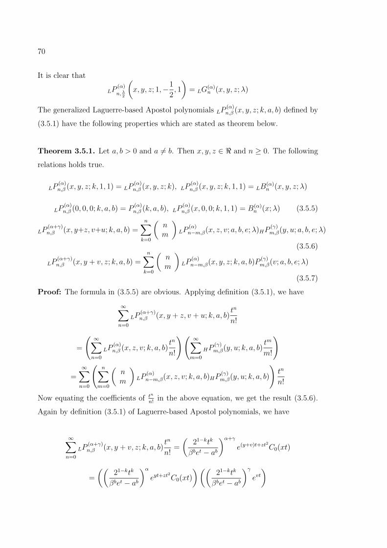
70

It is clear that

LP(α)

n,λ2

(x, y, z; 1,−1

2, 1

)= LG

(α)n (x, y, z;λ)

The generalized Laguerre-based Apostol polynomials LP(α)n,β (x, y, z; k, a, b) defined by

(3.5.1) have the following properties which are stated as theorem below.

Theorem 3.5.1. Let a, b > 0 and a 6= b. Then x, y, z ∈ < and n ≥ 0. The following

relations holds true.

LP(α)n,β (x, y, z; k, 1, 1) = LP

(α)n,β (x, y, z; k), LP

(α)n,β (x, y, z; k, 1, 1) = LB

(α)n (x, y, z;λ)

LP(α)n,β (0, 0, 0; k, a, b) = P

(α)n,β (k, a, b), LP

(α)n,β (x, 0, 0; k, 1, 1) = B(α)

n (x;λ) (3.5.5)

LP(α+γ)n,β (x, y+z, v+u; k, a, b) =

n∑k=0

(nm

)LP

(α)n−m,β(x, z, v; a, b, e;λ)HP

(γ)m,β(y, u; a, b, e;λ)

(3.5.6)

LP(α+γ)n,β (x, y + v, z; k, a, b) =

n∑k=0

(nm

)LP

(α)n−m,β(x, y, z; k, a, b)P

(γ)m,β(v; a, b, e;λ)

(3.5.7)

Proof: The formula in (3.5.5) are obvious. Applying definition (3.5.1), we have

∞∑n=0

LP(α+γ)n,β (x, y + z, v + u; k, a, b)

tn

n!

=

(∞∑n=0

LP(α)n,β (x, z, v; k, a, b)

tn

n!

)(∞∑m=0

HP(γ)m,β(y, u; k, a, b)

tm

m!

)

=∞∑n=0

(n∑

m=0

(nm

)LP

(α)n−m,β(x, z, v; k, a, b)HP

(γ)m,β(y, u; k, a, b)

)tn

n!

Now equating the coefficients of tn

n!in the above equation, we get the result (3.5.6).

Again by definition (3.5.1) of Laguerre-based Apostol polynomials, we have

∞∑n=0

LP(α+γ)n,β (x, y + v, z; k, a, b)

tn

n!=

(21−ktk

βbet − ab

)α+γ

e(y+v)t+zt2C0(xt)

=

((21−ktk

βbet − ab

)αeyt+zt

2

C0(xt)

)((21−ktk

βbet − ab

)γevt)

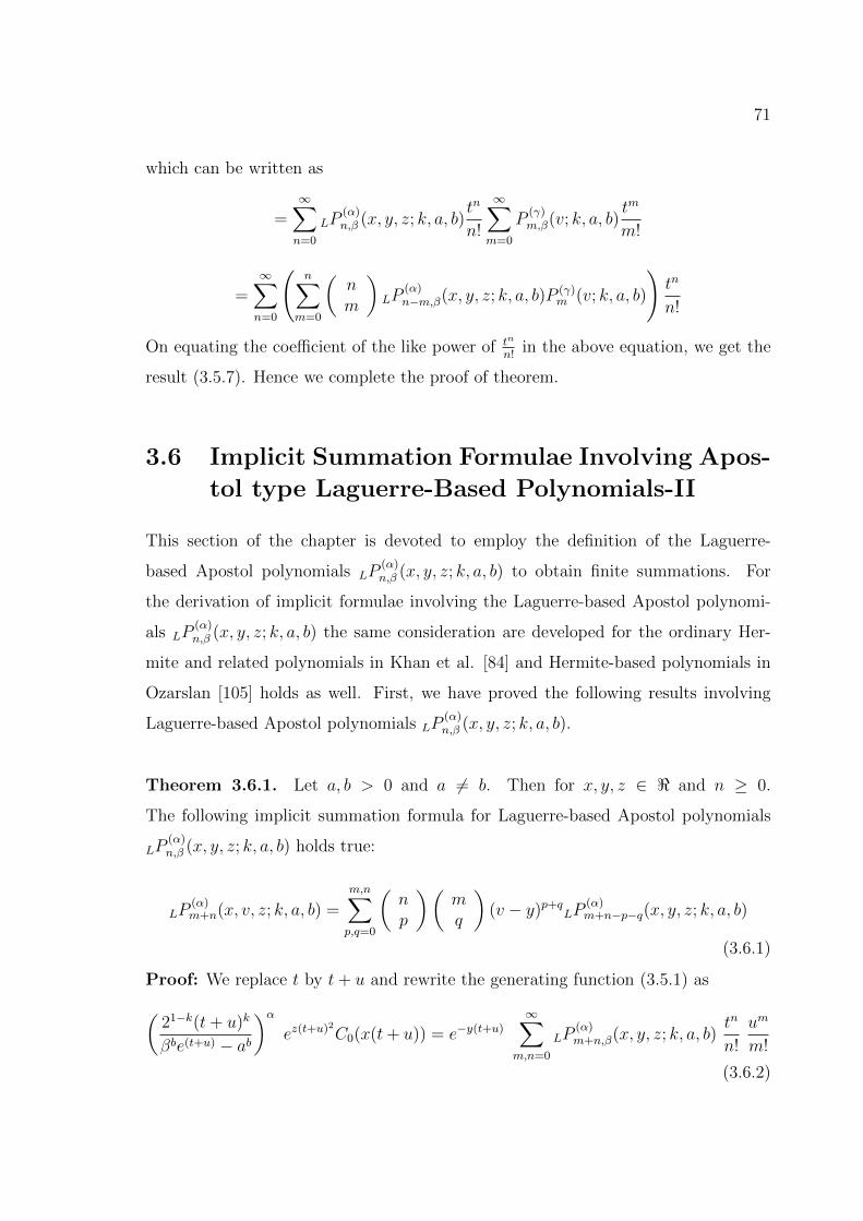
71

which can be written as

=∞∑n=0

LP(α)n,β (x, y, z; k, a, b)

tn

n!

∞∑m=0

P(γ)m,β(v; k, a, b)

tm

m!

=∞∑n=0

(n∑

m=0

(nm

)LP

(α)n−m,β(x, y, z; k, a, b)P (γ)

m (v; k, a, b)

)tn

n!

On equating the coefficient of the like power of tn

n!in the above equation, we get the

result (3.5.7). Hence we complete the proof of theorem.

3.6 Implicit Summation Formulae Involving Apos-

tol type Laguerre-Based Polynomials-II

This section of the chapter is devoted to employ the definition of the Laguerre-

based Apostol polynomials LP(α)n,β (x, y, z; k, a, b) to obtain finite summations. For

the derivation of implicit formulae involving the Laguerre-based Apostol polynomi-

als LP(α)n,β (x, y, z; k, a, b) the same consideration are developed for the ordinary Her-

mite and related polynomials in Khan et al. [84] and Hermite-based polynomials in

Ozarslan [105] holds as well. First, we have proved the following results involving

Laguerre-based Apostol polynomials LP(α)n,β (x, y, z; k, a, b).

Theorem 3.6.1. Let a, b > 0 and a 6= b. Then for x, y, z ∈ < and n ≥ 0.

The following implicit summation formula for Laguerre-based Apostol polynomials

LP(α)n,β (x, y, z; k, a, b) holds true:

LP(α)m+n(x, v, z; k, a, b) =

m,n∑p,q=0

(np

)(mq

)(v − y)p+qLP

(α)m+n−p−q(x, y, z; k, a, b)

(3.6.1)

Proof: We replace t by t+ u and rewrite the generating function (3.5.1) as(21−k(t+ u)k

βbe(t+u) − ab

)αez(t+u)2C0(x(t+ u)) = e−y(t+u)

∞∑m,n=0

LP(α)m+n,β(x, y, z; k, a, b)

tn

n!

um

m!

(3.6.2)

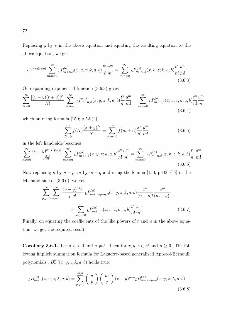
72

Replacing y by v in the above equation and equating the resulting equation to the

above equation, we get

e(v−y)(t+u)

∞∑m,n=0

LP(α)m+n,β(x, y, z; k, a, b)

tn

n!

um

m!=

∞∑m,n=0

LP(α)m+n,β(x, v, z; k, a, b)

tn

n!

um

m!

(3.6.3)

On expanding exponential function (3.6.3) gives

∞∑N=0

[(v − y)(t+ u)]N

N !

∞∑m,n=0

LP(α)m+n,β(x, y, z; k, a, b)

tn

n!

um

m!=

∞∑m,n=0

LP(α)m+n,β(x, v, z; k, a, b)

tn

n!

um

m!

(3.6.4)

which on using formula [150; p.52 (2)]

∞∑N=0

f(N)(x+ y)N

N !=

∞∑n,m=0

f(m+ n)xn

n!

ym

m!(3.6.5)

in the left hand side becomes∞∑

p,q=0

(v − y)p+q tpuq

p!q!

∞∑m,n=0

LP(α)m+n,β(x, y, z; k, a, b)

tn

n!

um

m!=

∞∑m,n=0

LP(α)m+n,β(x, v, z; k, a, b)

tn

n!

um

m!

(3.6.6)

Now replacing n by n − p, m by m − q and using the lemma [150; p.100 (1)] in the

left hand side of (3.6.6), we get

∞∑p,q=0

∞∑m,n=0

(v − y)p+q

p!q!LP

(α)m+n−p−q,β(x, y, z; k, a, b)

tn

(n− p)!um

(m− q)!

=∞∑

m,n=0

LP(α)m+n,β(x, v, z; k, a, b)

tn

n!

um

m!(3.6.7)

Finally, on equating the coefficients of the like powers of t and u in the above equa-

tion, we get the required result.

Corollary 3.6.1. Let a, b > 0 and a 6= b. Then for x, y, z ∈ < and n ≥ 0. The fol-

lowing implicit summation formula for Laguerre-based generalized Apostol-Bernoulli

polynomials LB(α)n (x, y, z;λ, a, b) holds true:

LB(α)m+n(x, v, z;λ, a, b) =

m,n∑p,q=0

(np

)(mq

)(v − y)p+qLB

(α)m+n−p−q(x, y, z;λ, a, b)

(3.6.8)

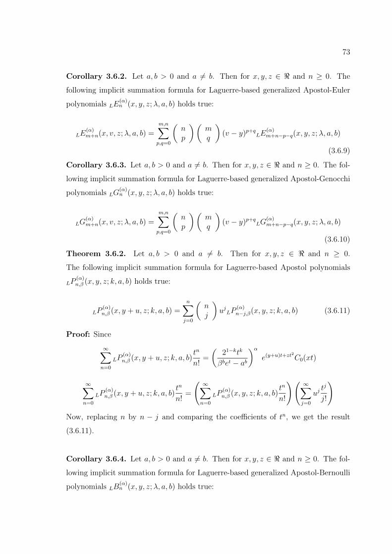
73

Corollary 3.6.2. Let a, b > 0 and a 6= b. Then for x, y, z ∈ < and n ≥ 0. The

following implicit summation formula for Laguerre-based generalized Apostol-Euler

polynomials LE(α)n (x, y, z;λ, a, b) holds true:

LE(α)m+n(x, v, z;λ, a, b) =

m,n∑p,q=0

(np

)(mq

)(v − y)p+qLE

(α)m+n−p−q(x, y, z;λ, a, b)

(3.6.9)

Corollary 3.6.3. Let a, b > 0 and a 6= b. Then for x, y, z ∈ < and n ≥ 0. The fol-

lowing implicit summation formula for Laguerre-based generalized Apostol-Genocchi

polynomials LG(α)n (x, y, z;λ, a, b) holds true:

LG(α)m+n(x, v, z;λ, a, b) =

m,n∑p,q=0

(np

)(mq

)(v − y)p+qLG

(α)m+n−p−q(x, y, z;λ, a, b)

(3.6.10)

Theorem 3.6.2. Let a, b > 0 and a 6= b. Then for x, y, z ∈ < and n ≥ 0.

The following implicit summation formula for Laguerre-based Apostol polynomials

LP(α)n,β (x, y, z; k, a, b) holds true:

LP(α)n,β (x, y + u, z; k, a, b) =

n∑j=0

(nj

)ujLP

(α)n−j,β(x, y, z; k, a, b) (3.6.11)

Proof: Since

∞∑n=0

LP(α)n,β (x, y + u, z; k, a, b)

tn

n!=

(21−ktk

βbet − ab

)αe(y+u)t+zt2C0(xt)

∞∑n=0

LP(α)n,β (x, y + u, z; k, a, b)

tn

n!=

(∞∑n=0

LP(α)n,β (x, y, z; k, a, b)

tn

n!

)(∞∑j=0

ujtj

j!

)

Now, replacing n by n − j and comparing the coefficients of tn, we get the result

(3.6.11).

Corollary 3.6.4. Let a, b > 0 and a 6= b. Then for x, y, z ∈ < and n ≥ 0. The fol-

lowing implicit summation formula for Laguerre-based generalized Apostol-Bernoulli

polynomials LB(α)n (x, y, z;λ, a, b) holds true:

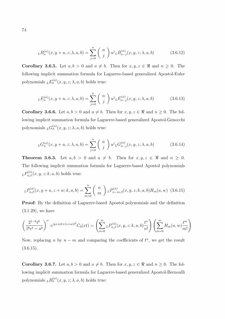
74

LB(α)n (x, y + u, z;λ, a, b) =

n∑j=0

(nj

)ujLB

(α)n−j(x, y, z;λ, a, b) (3.6.12)

Corollary 3.6.5. Let a, b > 0 and a 6= b. Then for x, y, z ∈ < and n ≥ 0. The

following implicit summation formula for Laguerre-based generalized Apostol-Euler

polynomials LE(α)n (x, y, z;λ, a, b) holds true:

LE(α)n (x, y + u, z;λ, a, b) =

n∑j=0

(nj

)ujLE

(α)n−j(x, y, z;λ, a, b) (3.6.13)

Corollary 3.6.6. Let a, b > 0 and a 6= b. Then for x, y, z ∈ < and n ≥ 0. The fol-

lowing implicit summation formula for Laguerre-based generalized Apostol-Genocchi

polynomials LG(α)n (x, y, z;λ, a, b) holds true:

LG(α)n (x, y + u, z;λ, a, b) =

n∑j=0

(nj

)ujLG

(α)n−j(x, y, z;λ, a, b) (3.6.14)

Theorem 3.6.3. Let a, b > 0 and a 6= b. Then for x, y, z ∈ < and n ≥ 0.

The following implicit summation formula for Laguerre-based Apostol polynomials

LP(α)n,β (x, y, z; k, a, b) holds true:

LP(α)n,β (x, y + u, z + w; k, a, b) =

n∑m=0

(nm

)LP

(α)n−m,β(x, y, z; k, a, b)Hm(u,w) (3.6.15)

Proof: By the definition of Laguerre-based Apostol polynomials and the definition

(3.1.29), we have(21−ktk

βbet − ab

)αe(y+u)t+(z+w)t2C0(xt) =

(∞∑n=0

LP(α)n,β (x, y, z; k, a, b)

tn

n!

)(∞∑m=0

Hm(u,w)tm

m!

)

Now, replacing n by n − m and comparing the coefficients of tn, we get the result

(3.6.15).

Corollary 3.6.7. Let a, b > 0 and a 6= b. Then for x, y, z ∈ < and n ≥ 0. The fol-

lowing implicit summation formula for Laguerre-based generalized Apostol-Bernoulli

polynomials LB(α)n (x, y, z;λ, a, b) holds true:

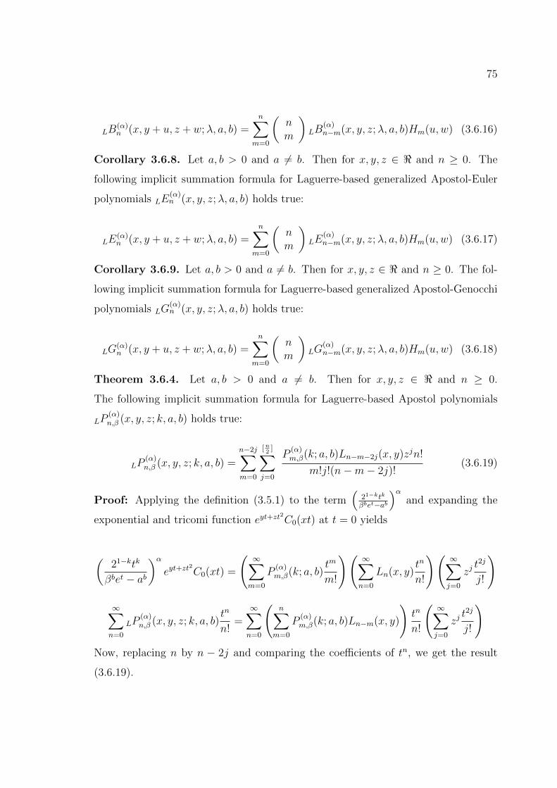
75

LB(α)n (x, y + u, z + w;λ, a, b) =

n∑m=0

(nm

)LB

(α)n−m(x, y, z;λ, a, b)Hm(u,w) (3.6.16)

Corollary 3.6.8. Let a, b > 0 and a 6= b. Then for x, y, z ∈ < and n ≥ 0. The

following implicit summation formula for Laguerre-based generalized Apostol-Euler

polynomials LE(α)n (x, y, z;λ, a, b) holds true:

LE(α)n (x, y + u, z + w;λ, a, b) =

n∑m=0

(nm

)LE

(α)n−m(x, y, z;λ, a, b)Hm(u,w) (3.6.17)

Corollary 3.6.9. Let a, b > 0 and a 6= b. Then for x, y, z ∈ < and n ≥ 0. The fol-

lowing implicit summation formula for Laguerre-based generalized Apostol-Genocchi

polynomials LG(α)n (x, y, z;λ, a, b) holds true:

LG(α)n (x, y + u, z + w;λ, a, b) =

n∑m=0

(nm

)LG

(α)n−m(x, y, z;λ, a, b)Hm(u,w) (3.6.18)

Theorem 3.6.4. Let a, b > 0 and a 6= b. Then for x, y, z ∈ < and n ≥ 0.

The following implicit summation formula for Laguerre-based Apostol polynomials

LP(α)n,β (x, y, z; k, a, b) holds true:

LP(α)n,β (x, y, z; k, a, b) =

n−2j∑m=0

[n2

]∑j=0

P(α)m,β(k; a, b)Ln−m−2j(x, y)zjn!

m!j!(n−m− 2j)!(3.6.19)

Proof: Applying the definition (3.5.1) to the term(

21−ktk

βbet−ab

)αand expanding the

exponential and tricomi function eyt+zt2C0(xt) at t = 0 yields

(21−ktk

βbet − ab

)αeyt+zt

2

C0(xt) =

(∞∑m=0

P(α)m,β(k; a, b)

tm

m!

)(∞∑n=0

Ln(x, y)tn

n!

)(∞∑j=0

zjt2j

j!

)

∞∑n=0

LP(α)n,β (x, y, z; k, a, b)

tn

n!=∞∑n=0

(n∑

m=0

P(α)m,β(k; a, b)Ln−m(x, y)

)tn

n!

(∞∑j=0

zjt2j

j!

)Now, replacing n by n − 2j and comparing the coefficients of tn, we get the result

(3.6.19).

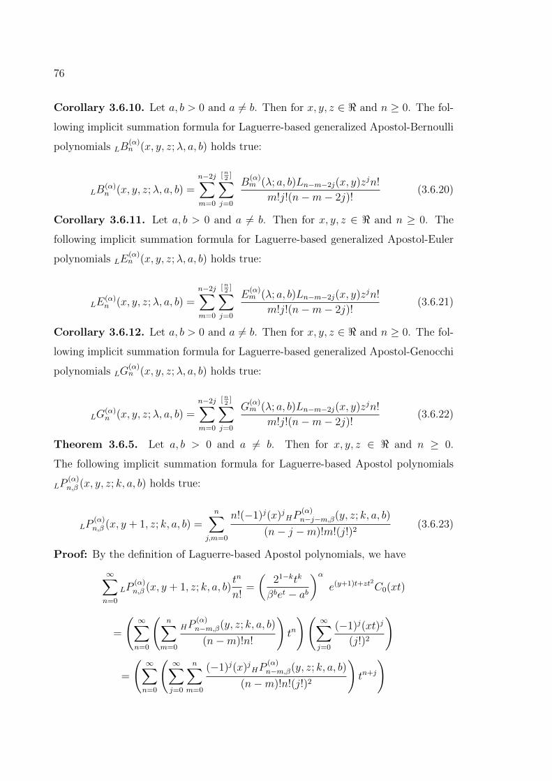
76

Corollary 3.6.10. Let a, b > 0 and a 6= b. Then for x, y, z ∈ < and n ≥ 0. The fol-

lowing implicit summation formula for Laguerre-based generalized Apostol-Bernoulli

polynomials LB(α)n (x, y, z;λ, a, b) holds true:

LB(α)n (x, y, z;λ, a, b) =

n−2j∑m=0

[n2

]∑j=0

B(α)m (λ; a, b)Ln−m−2j(x, y)zjn!

m!j!(n−m− 2j)!(3.6.20)

Corollary 3.6.11. Let a, b > 0 and a 6= b. Then for x, y, z ∈ < and n ≥ 0. The

following implicit summation formula for Laguerre-based generalized Apostol-Euler

polynomials LE(α)n (x, y, z;λ, a, b) holds true:

LE(α)n (x, y, z;λ, a, b) =

n−2j∑m=0

[n2

]∑j=0

E(α)m (λ; a, b)Ln−m−2j(x, y)zjn!

m!j!(n−m− 2j)!(3.6.21)

Corollary 3.6.12. Let a, b > 0 and a 6= b. Then for x, y, z ∈ < and n ≥ 0. The fol-

lowing implicit summation formula for Laguerre-based generalized Apostol-Genocchi

polynomials LG(α)n (x, y, z;λ, a, b) holds true:

LG(α)n (x, y, z;λ, a, b) =

n−2j∑m=0

[n2

]∑j=0

G(α)m (λ; a, b)Ln−m−2j(x, y)zjn!

m!j!(n−m− 2j)!(3.6.22)

Theorem 3.6.5. Let a, b > 0 and a 6= b. Then for x, y, z ∈ < and n ≥ 0.

The following implicit summation formula for Laguerre-based Apostol polynomials

LP(α)n,β (x, y, z; k, a, b) holds true:

LP(α)n,β (x, y + 1, z; k, a, b) =

n∑j,m=0

n!(−1)j(x)jHP(α)n−j−m,β(y, z; k, a, b)

(n− j −m)!m!(j!)2(3.6.23)

Proof: By the definition of Laguerre-based Apostol polynomials, we have

∞∑n=0

LP(α)n,β (x, y + 1, z; k, a, b)

tn

n!=

(21−ktk

βbet − ab

)αe(y+1)t+zt2C0(xt)

=

(∞∑n=0

(n∑

m=0

HP(α)n−m,β(y, z; k, a, b)

(n−m)!n!

)tn

)(∞∑j=0

(−1)j(xt)j

(j!)2

)

=

(∞∑n=0

(∞∑j=0

n∑m=0

(−1)j(x)jHP(α)n−m,β(y, z; k, a, b)

(n−m)!n!(j!)2

)tn+j

)

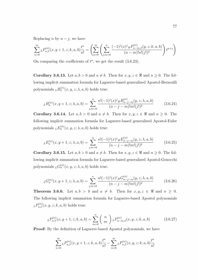
77

Replacing n by n− j, we have

∞∑n=0

LP(α)n,β (x, y + 1, z; k, a, b)

tn

n!=

(∞∑n=0

(n∑

j,m=0

(−1)j(x)jHP(α)n−m,β(y, z; k, a, b)

(n−m)!n!(j!)2

)tn+j

)On comparing the coefficients of tn, we get the result (3.6.23).

Corollary 3.6.13. Let a, b > 0 and a 6= b. Then for x, y, z ∈ < and n ≥ 0. The fol-

lowing implicit summation formula for Laguerre-based generalized Apostol-Bernoulli

polynomials LB(α)n (x, y, z;λ, a, b) holds true:

LB(α)n (x, y + 1, z;λ, a, b) =

n∑j,m=0

n!(−1)j(x)jHB(α)n−j−m(y, z;λ, a, b)

(n− j −m)!m!(j!)2(3.6.24)

Corollary 3.6.14. Let a, b > 0 and a 6= b. Then for x, y, z ∈ < and n ≥ 0. The

following implicit summation formula for Laguerre-based generalized Apostol-Euler

polynomials LE(α)n (x, y, z;λ, a, b) holds true:

LE(α)n (x, y + 1, z;λ, a, b) =

n∑j,m=0

n!(−1)j(x)jHE(α)n−j−m(y, z;λ, a, b)

(n− j −m)!m!(j!)2(3.6.25)

Corollary 3.6.15. Let a, b > 0 and a 6= b. Then for x, y, z ∈ < and n ≥ 0. The fol-

lowing implicit summation formula for Laguerre-based generalized Apostol-Genocchi

polynomials LG(α)n (x, y, z;λ, a, b) holds true:

LG(α)n (x, y + 1, z;λ, a, b) =

n∑j,m=0

n!(−1)j(x)jHG(α)n−j−m(y, z;λ, a, b)

(n− j −m)!m!(j!)2(3.6.26)

Theorem 3.6.6. Let a, b > 0 and a 6= b. Then for x, y, z ∈ < and n ≥ 0.

The following implicit summation formula for Laguerre-based Apostol polynomials

LP(α)n,β (x, y, z; k, a, b) holds true:

LP(α)n,β (x, y + 1, z; k, a, b) =

n∑m=0

(nm

)LP

(α)n−m,β(x, y, z; k, a, b) (3.6.27)

Proof: By the definition of Laguerre-based Apostol polynomials, we have

∞∑n=0

LP(α)n,β (x, y + 1, z; k, a, b)

tn

n!−∞∑n=0

LP(α)n,β (x, y, z; k, a, b)

tn

n!

78

=

(21−ktk

βbet − ab

)α(et − 1)eyt+zt

2

C0(xt)

=∞∑n=0

LP(α)n,β (x, y, z; k, a, b)

tn

n!

(∞∑m=0

tm

m!− 1

)

=∞∑n=0

LP(α)n (x, y, z; k, a, b)

tn

n!

∞∑m=0

tm

m!−∞∑n=0

LE(α)n,β(x, y, z; k, a, b)

tn

n!

=∞∑n=0

n∑m=0

LP(α)n−m,β(x, y, z; k, a, b)

tn

m!(n−m)!−∞∑n=0

LP(α)n,β (x, y, z; k, a, b)

tn

n!

Finally equating the coefficients of the like powers of tn, we get the result (3.6.27).

Corollary 3.6.16. Let a, b > 0 and a 6= b. Then for x, y, z ∈ < and n ≥ 0. The fol-

lowing implicit summation formula for Laguerre-based generalized Apostol-Bernoulli

polynomials LB(α)n (x, y, z;λ, a, b) holds true:

LB(α)n (x, y + 1, z;λ, a, b) =

n∑m=0

(nm

)LB

(α)n−m(x, y, z;λ, a, b) (3.6.28)

Corollary 3.6.17. Let a, b > 0 and a 6= b. Then for x, y, z ∈ < and n ≥ 0. The

following implicit summation formula for Laguerre-based generalized Apostol-Euler

polynomials LE(α)n (x, y, z;λ, a, b) holds true:

LE(α)n (x, y + 1, z;λ, a, b) =

n∑m=0

(nm

)LE

(α)n−m(x, y, z;λ, a, b) (3.6.29)

Corollary 3.6.18. Let a, b > 0 and a 6= b. Then for x, y, z ∈ < and n ≥ 0. The fol-

lowing implicit summation formula for Laguerre-based generalized Apostol-Genocchi

polynomials LG(α)n (x, y, z;λ, a, b) holds true:

LG(α)n (x, y + 1, z;λ, a, b) =

n∑m=0

(nm

)LG

(α)n−m(x, y, z;λ, a, b) (3.6.30)

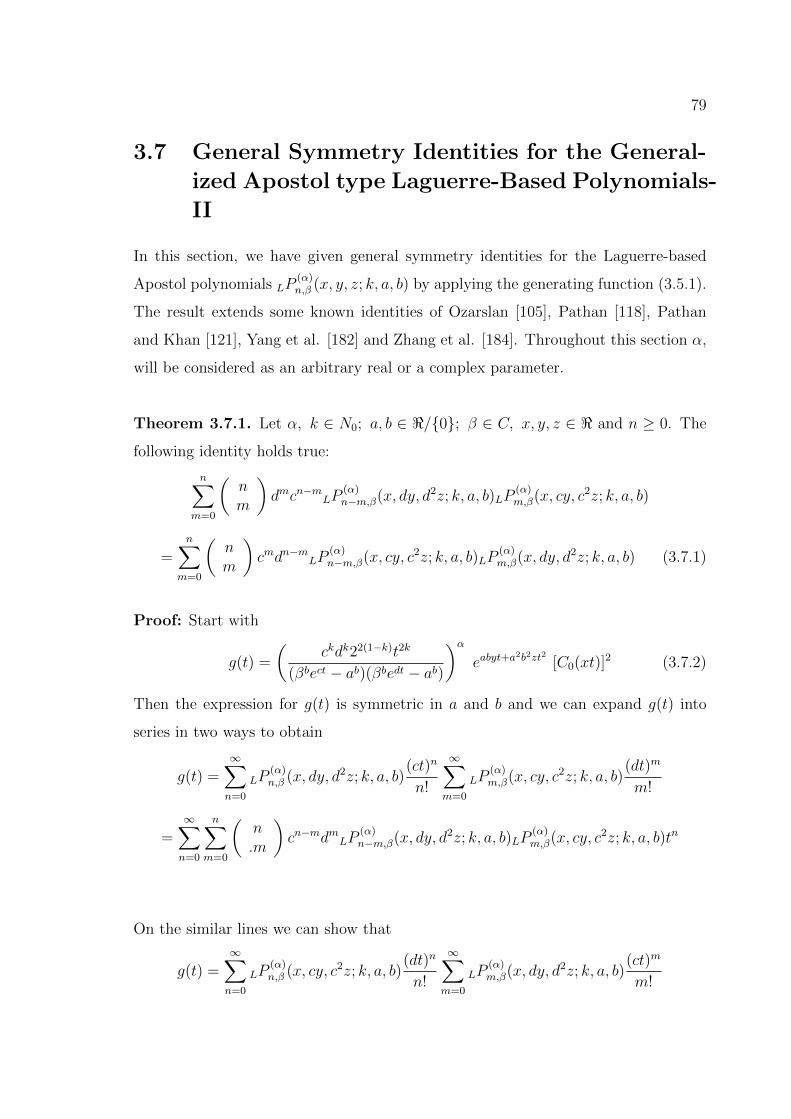
79

3.7 General Symmetry Identities for the General-

ized Apostol type Laguerre-Based Polynomials-

II

In this section, we have given general symmetry identities for the Laguerre-based

Apostol polynomials LP(α)n,β (x, y, z; k, a, b) by applying the generating function (3.5.1).

The result extends some known identities of Ozarslan [105], Pathan [118], Pathan

and Khan [121], Yang et al. [182] and Zhang et al. [184]. Throughout this section α,

will be considered as an arbitrary real or a complex parameter.

Theorem 3.7.1. Let α, k ∈ N0; a, b ∈ </0; β ∈ C, x, y, z ∈ < and n ≥ 0. The

following identity holds true:

n∑m=0

(nm

)dmcn−mLP

(α)n−m,β(x, dy, d2z; k, a, b)LP

(α)m,β(x, cy, c2z; k, a, b)

=n∑

m=0

(nm

)cmdn−mLP

(α)n−m,β(x, cy, c2z; k, a, b)LP

(α)m,β(x, dy, d2z; k, a, b) (3.7.1)

Proof: Start with

g(t) =

(ckdk22(1−k)t2k

(βbect − ab)(βbedt − ab)

)αeabyt+a

2b2zt2 [C0(xt)]2 (3.7.2)

Then the expression for g(t) is symmetric in a and b and we can expand g(t) into

series in two ways to obtain

g(t) =∞∑n=0

LP(α)n,β (x, dy, d2z; k, a, b)

(ct)n

n!

∞∑m=0

LP(α)m,β(x, cy, c2z; k, a, b)

(dt)m

m!

=∞∑n=0

n∑m=0

(n.m

)cn−mdmLP

(α)n−m,β(x, dy, d2z; k, a, b)LP

(α)m,β(x, cy, c2z; k, a, b)tn

On the similar lines we can show that

g(t) =∞∑n=0

LP(α)n,β (x, cy, c2z; k, a, b)

(dt)n

n!

∞∑m=0

LP(α)m,β(x, dy, d2z; k, a, b)

(ct)m

m!

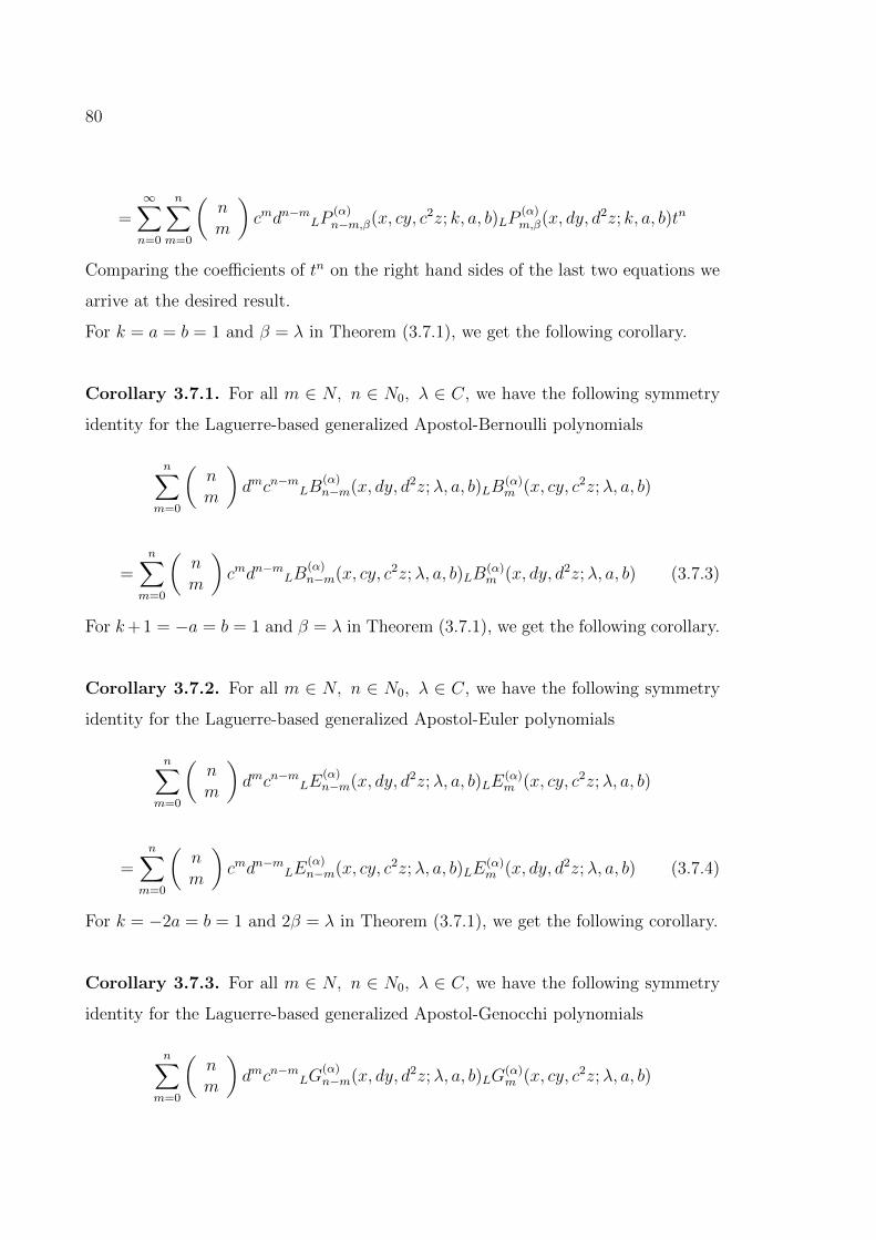
80

=∞∑n=0

n∑m=0

(nm

)cmdn−mLP

(α)n−m,β(x, cy, c2z; k, a, b)LP

(α)m,β(x, dy, d2z; k, a, b)tn

Comparing the coefficients of tn on the right hand sides of the last two equations we

arrive at the desired result.

For k = a = b = 1 and β = λ in Theorem (3.7.1), we get the following corollary.

Corollary 3.7.1. For all m ∈ N, n ∈ N0, λ ∈ C, we have the following symmetry

identity for the Laguerre-based generalized Apostol-Bernoulli polynomials

n∑m=0

(nm

)dmcn−mLB

(α)n−m(x, dy, d2z;λ, a, b)LB

(α)m (x, cy, c2z;λ, a, b)

=n∑

m=0

(nm

)cmdn−mLB

(α)n−m(x, cy, c2z;λ, a, b)LB

(α)m (x, dy, d2z;λ, a, b) (3.7.3)

For k+ 1 = −a = b = 1 and β = λ in Theorem (3.7.1), we get the following corollary.

Corollary 3.7.2. For all m ∈ N, n ∈ N0, λ ∈ C, we have the following symmetry

identity for the Laguerre-based generalized Apostol-Euler polynomials

n∑m=0

(nm

)dmcn−mLE

(α)n−m(x, dy, d2z;λ, a, b)LE

(α)m (x, cy, c2z;λ, a, b)

=n∑

m=0

(nm

)cmdn−mLE

(α)n−m(x, cy, c2z;λ, a, b)LE

(α)m (x, dy, d2z;λ, a, b) (3.7.4)

For k = −2a = b = 1 and 2β = λ in Theorem (3.7.1), we get the following corollary.

Corollary 3.7.3. For all m ∈ N, n ∈ N0, λ ∈ C, we have the following symmetry

identity for the Laguerre-based generalized Apostol-Genocchi polynomials

n∑m=0

(nm

)dmcn−mLG

(α)n−m(x, dy, d2z;λ, a, b)LG

(α)m (x, cy, c2z;λ, a, b)

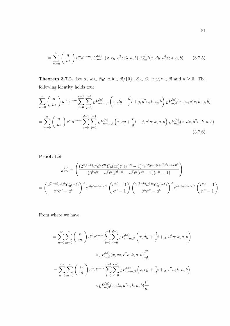
81

=n∑

m=0

(nm

)cmdn−mLG

(α)n−m(x, cy, c2z;λ, a, b)LG

(α)m (x, dy, d2z;λ, a, b) (3.7.5)

Theorem 3.7.2. Let α, k ∈ N0; a, b ∈ </0; β ∈ C, x, y, z ∈ < and n ≥ 0. The

following identity holds true:

n∑m=0

(nm

)dmcn−m

c−1∑i=0

d−1∑j=0

LP(α)n−m,β

(x, dy +

d

ci+ j, d2u; k, a, b

)LP

(α)m,β(x, cz, c2v; k, a, b)

=n∑

m=0

(nm

)cmdn−m

d−1∑i=0

c−1∑j=0

LP(α)n−m,β

(x, cy +

c

di+ j, c2u; k, a, b

)LP

(α)m,β(x, dz, d2v; k, a, b)

(3.7.6)

Proof: Let

g(t) =

((22(1−k)ckdkt2kC0(xt))α(ecdt − 1)2ecd(y+z)t+c2d2(u+v)t2

(βbect − ab)α(βbedt − ab)α(ect − 1)(edt − 1)

)

=

(2(1−k)cktkC0(xt)

βbect − ab

)αecdyt+c

2d2ut2(ecdt − 1

ect − 1

)(2(1−k)dktkC0(xt)

βbedt − ab

)αecdzt+c

2d2vt2(ecdt − 1

edt − 1

)

From where we have

=∞∑n=0

n∑m=0

(nm

)dmcn−m

c−1∑i=0

d−1∑j=0

LP(α)n−m,β

(x, dy +

d

ci+ j, d2u; k, a, b

)

×LP (α)m,β(x, cz, c2v; k, a, b)

tn

n!

=∞∑n=0

n∑m=0

(nm

)cmdn−m

d−1∑i=0

c−1∑j=0

LP(α)n−m,β

(x, cy +

c

di+ j, c2u; k, a, b

)×LP (α)

m,β(x, dz, d2v; k, a, b)tn

n!

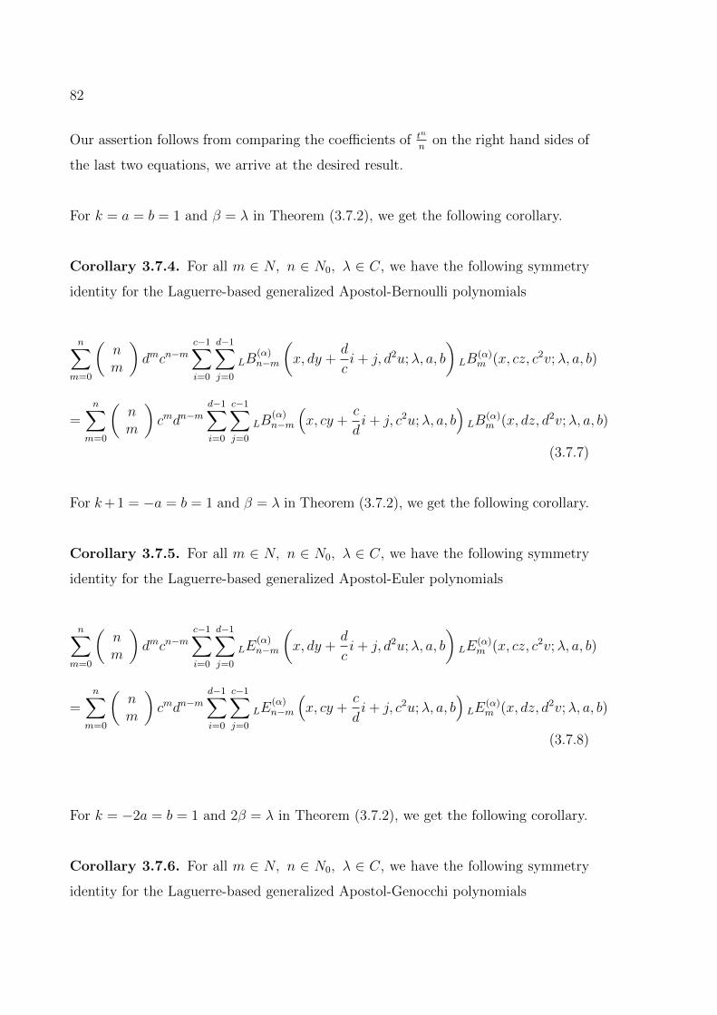
82

Our assertion follows from comparing the coefficients of tn

non the right hand sides of

the last two equations, we arrive at the desired result.

For k = a = b = 1 and β = λ in Theorem (3.7.2), we get the following corollary.

Corollary 3.7.4. For all m ∈ N, n ∈ N0, λ ∈ C, we have the following symmetry

identity for the Laguerre-based generalized Apostol-Bernoulli polynomials

n∑m=0

(nm

)dmcn−m

c−1∑i=0

d−1∑j=0

LB(α)n−m

(x, dy +

d

ci+ j, d2u;λ, a, b

)LB

(α)m (x, cz, c2v;λ, a, b)

=n∑

m=0

(nm

)cmdn−m

d−1∑i=0

c−1∑j=0

LB(α)n−m

(x, cy +

c

di+ j, c2u;λ, a, b

)LB

(α)m (x, dz, d2v;λ, a, b)

(3.7.7)

For k+ 1 = −a = b = 1 and β = λ in Theorem (3.7.2), we get the following corollary.

Corollary 3.7.5. For all m ∈ N, n ∈ N0, λ ∈ C, we have the following symmetry

identity for the Laguerre-based generalized Apostol-Euler polynomials

n∑m=0

(nm

)dmcn−m

c−1∑i=0

d−1∑j=0

LE(α)n−m

(x, dy +

d

ci+ j, d2u;λ, a, b

)LE

(α)m (x, cz, c2v;λ, a, b)

=n∑

m=0

(nm

)cmdn−m

d−1∑i=0

c−1∑j=0

LE(α)n−m

(x, cy +

c

di+ j, c2u;λ, a, b

)LE

(α)m (x, dz, d2v;λ, a, b)

(3.7.8)

For k = −2a = b = 1 and 2β = λ in Theorem (3.7.2), we get the following corollary.

Corollary 3.7.6. For all m ∈ N, n ∈ N0, λ ∈ C, we have the following symmetry

identity for the Laguerre-based generalized Apostol-Genocchi polynomials

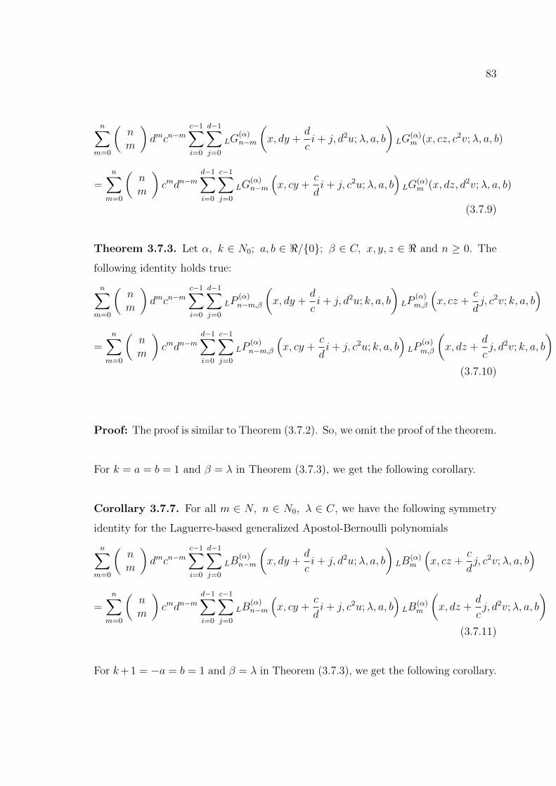
83

n∑m=0

(nm

)dmcn−m

c−1∑i=0

d−1∑j=0

LG(α)n−m

(x, dy +

d

ci+ j, d2u;λ, a, b

)LG

(α)m (x, cz, c2v;λ, a, b)

=n∑

m=0

(nm

)cmdn−m

d−1∑i=0

c−1∑j=0

LG(α)n−m

(x, cy +

c

di+ j, c2u;λ, a, b

)LG

(α)m (x, dz, d2v;λ, a, b)

(3.7.9)

Theorem 3.7.3. Let α, k ∈ N0; a, b ∈ </0; β ∈ C, x, y, z ∈ < and n ≥ 0. The

following identity holds true:

n∑m=0

(nm

)dmcn−m

c−1∑i=0

d−1∑j=0

LP(α)n−m,β

(x, dy +

d

ci+ j, d2u; k, a, b

)LP

(α)m,β

(x, cz +

c

dj, c2v; k, a, b

)

=n∑

m=0

(nm

)cmdn−m

d−1∑i=0

c−1∑j=0

LP(α)n−m,β

(x, cy +

c

di+ j, c2u; k, a, b

)LP

(α)m,β

(x, dz +

d

cj, d2v; k, a, b

)(3.7.10)

Proof: The proof is similar to Theorem (3.7.2). So, we omit the proof of the theorem.

For k = a = b = 1 and β = λ in Theorem (3.7.3), we get the following corollary.

Corollary 3.7.7. For all m ∈ N, n ∈ N0, λ ∈ C, we have the following symmetry

identity for the Laguerre-based generalized Apostol-Bernoulli polynomials

n∑m=0

(nm

)dmcn−m

c−1∑i=0

d−1∑j=0

LB(α)n−m

(x, dy +

d

ci+ j, d2u;λ, a, b

)LB

(α)m

(x, cz +

c

dj, c2v;λ, a, b

)

=n∑

m=0

(nm

)cmdn−m

d−1∑i=0

c−1∑j=0

LB(α)n−m

(x, cy +

c

di+ j, c2u;λ, a, b

)LB

(α)m

(x, dz +

d

cj, d2v;λ, a, b

)(3.7.11)

For k+ 1 = −a = b = 1 and β = λ in Theorem (3.7.3), we get the following corollary.

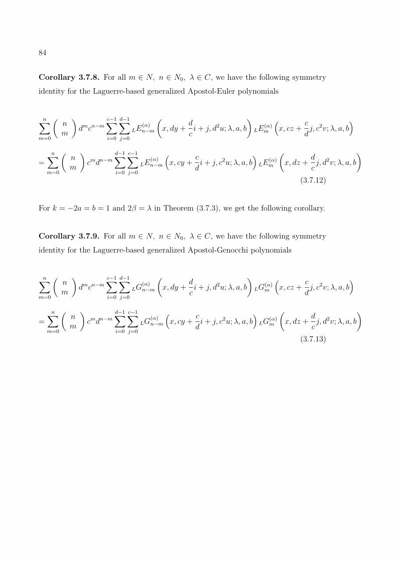
84

Corollary 3.7.8. For all m ∈ N, n ∈ N0, λ ∈ C, we have the following symmetry

identity for the Laguerre-based generalized Apostol-Euler polynomials

n∑m=0

(nm

)dmcn−m

c−1∑i=0

d−1∑j=0

LE(α)n−m

(x, dy +

d

ci+ j, d2u;λ, a, b

)LE

(α)m

(x, cz +

c

dj, c2v;λ, a, b

)

=n∑

m=0

(nm

)cmdn−m

d−1∑i=0

c−1∑j=0

LE(α)n−m

(x, cy +

c

di+ j, c2u;λ, a, b

)LE

(α)m

(x, dz +

d

cj, d2v;λ, a, b

)(3.7.12)

For k = −2a = b = 1 and 2β = λ in Theorem (3.7.3), we get the following corollary.

Corollary 3.7.9. For all m ∈ N, n ∈ N0, λ ∈ C, we have the following symmetry

identity for the Laguerre-based generalized Apostol-Genocchi polynomials

n∑m=0

(nm

)dmcn−m

c−1∑i=0

d−1∑j=0

LG(α)n−m

(x, dy +

d

ci+ j, d2u;λ, a, b

)LG

(α)m

(x, cz +

c

dj, c2v;λ, a, b

)

=n∑

m=0

(nm

)cmdn−m

d−1∑i=0

c−1∑j=0

LG(α)n−m

(x, cy +

c

di+ j, c2u;λ, a, b

)LG

(α)m

(x, dz +

d

cj, d2v;λ, a, b

)(3.7.13)

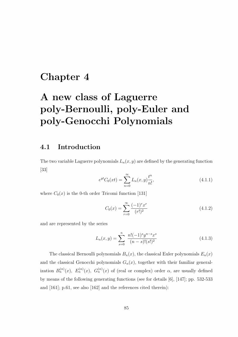
Chapter 4

A new class of Laguerrepoly-Bernoulli, poly-Euler andpoly-Genocchi Polynomials

4.1 Introduction

The two variable Laguerre polynomials Ln(x, y) are defined by the generating function

[33]

eytC0(xt) =∞∑n=0

Ln(x, y)tn

n!, (4.1.1)

where C0(x) is the 0-th order Tricomi function [131]

C0(x) =∞∑r=0

(−1)rxr

(r!)2(4.1.2)

and are represented by the series

Ln(x, y) =n∑s=0

n!(−1)syn−sxs

(n− s)!(s!)2(4.1.3)

The classical Bernoulli polynomials Bn(x), the classical Euler polynomials En(x)

and the classical Genocchi polynomials Gn(x), together with their familiar general-

ization B(α)n (x), E

(α)n (x), G

(α)n (x) of (real or complex) order α, are usually defined

by means of the following generating functions (see for details [6], [147]; pp. 532-533

and [161]; p.61, see also [162] and the references cited therein):

85

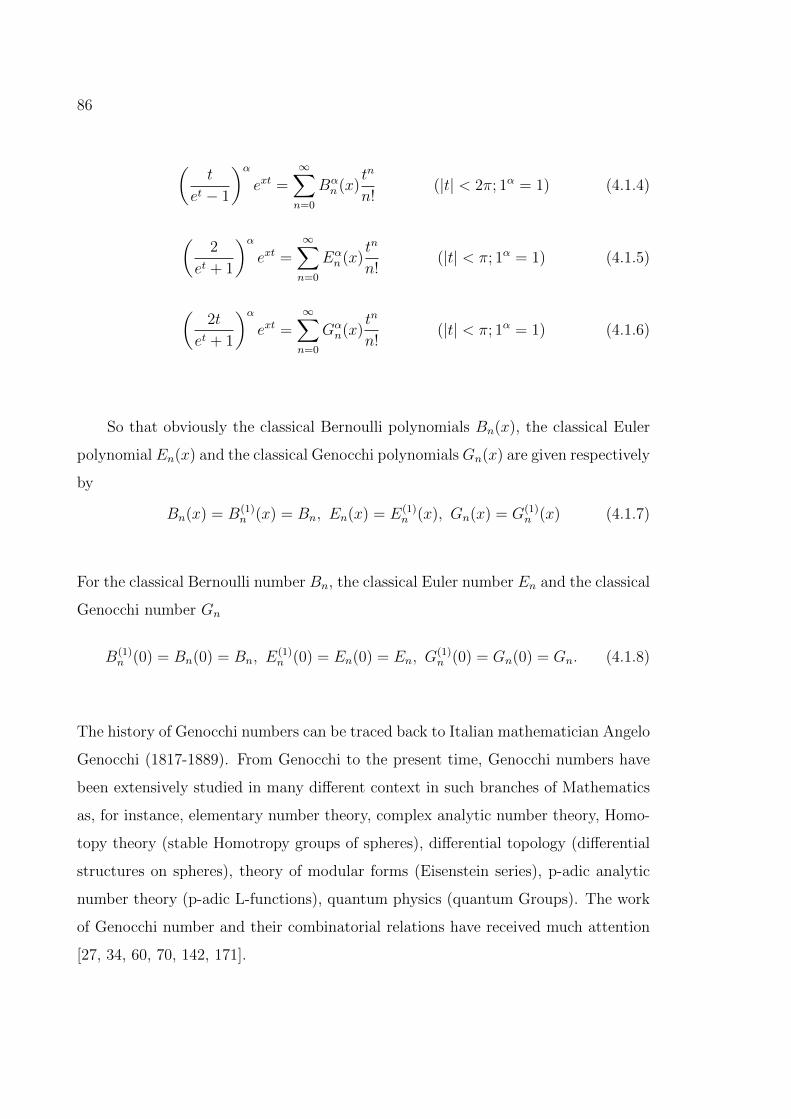
86

(t

et − 1

)αext =

∞∑n=0

Bαn (x)

tn

n!(|t| < 2π; 1α = 1) (4.1.4)

(2

et + 1

)αext =

∞∑n=0

Eαn (x)

tn

n!(|t| < π; 1α = 1) (4.1.5)

(2t

et + 1

)αext =

∞∑n=0

Gαn(x)

tn

n!(|t| < π; 1α = 1) (4.1.6)

So that obviously the classical Bernoulli polynomials Bn(x), the classical Euler

polynomial En(x) and the classical Genocchi polynomialsGn(x) are given respectively

by

Bn(x) = B(1)n (x) = Bn, En(x) = E(1)

n (x), Gn(x) = G(1)n (x) (4.1.7)

For the classical Bernoulli number Bn, the classical Euler number En and the classical

Genocchi number Gn

B(1)n (0) = Bn(0) = Bn, E

(1)n (0) = En(0) = En, G

(1)n (0) = Gn(0) = Gn. (4.1.8)

The history of Genocchi numbers can be traced back to Italian mathematician Angelo

Genocchi (1817-1889). From Genocchi to the present time, Genocchi numbers have

been extensively studied in many different context in such branches of Mathematics

as, for instance, elementary number theory, complex analytic number theory, Homo-

topy theory (stable Homotropy groups of spheres), differential topology (differential

structures on spheres), theory of modular forms (Eisenstein series), p-adic analytic

number theory (p-adic L-functions), quantum physics (quantum Groups). The work

of Genocchi number and their combinatorial relations have received much attention

[27, 34, 60, 70, 142, 171].

87

In [65], Kaneko introduced and studied poly-Bernoulli numbers which generalizes

the classical Bernoulli numbers. poly-Bernoulli numbers Bn(k) with k ∈ z and n ∈ N ,

appear in the following power series

Lik(1− e−t)1− e−t

=∞∑n=0

B(k)n

tn

n!(4.1.9)

where k ∈ z and

Lik =∞∑m=1

zm

m!, |z| < 1

so for k ≤ 1,

Lik = −ln(1− z), Li0(z) =z

1− z, Li−1 =

z

(1− z)2, · · ·

Moreover when k ≤ 1, the left hand side of (4.1.9) can be written in the form

et1

et − 1

∫ t

0

1

et − 1· · ·∫ t

0

1

et − 1

∫ t

0

1

et − 1dtdt · · · dt =

∞∑n=0

B(k)n

tn

n!

In the special case, one can see

B(1)n = Bn.

Recently, Jolany et al. [61-64] generalized the concept of poly-Bernoulli polynomials

is defined as follows.

Let a, b, c > 0 and a 6= b. The generalized poly-Bernoulli numbers B(k)n (a, b), the

generalized poly-Bernoulli polynomialsB(k)n (x, a, b) and the polynomialsB

(k)n (x, a, b, c)

are appeared in the following series respectively

Lik(1− (ab)−t)

bt − a−t=∞∑n=0

B(k)n (a, b)

tn

n!, |t| < 2π

|lna + lnb|(4.1.10)

Lik(1− (ab)−t)

bt − a−text =

∞∑n=0

B(k)n (x, a, b)

tn

n!, |t| < 2π

|lna + lnb|(4.1.11)

Lik(1− (ab)−t)

bt − a−tcxt =

∞∑n=0

B(k)n (x, a, b, c)

tn

n!, |t| < 2π

|lna + lnb|(4.1.12)

88

One can easily see that

B(k)n (0, 1, e) = B(k)

n , B(k)n (x) = 1 + x

and

B(k)n (x) = B(k)

n (ex+1, ex) (4.1.13)

where B(k)n are generalized poly-Bernoulli numbers. For more information about poly-

Bernoulli numbers and poly-Bernoulli polynomials, we refer to (see [58-59, 61-64]).

Recently, the generalized poly-Euler polynomials are defined by Jolany et al.

[61-64] as follows:

2Lik(1− (ab)−t)

a−t + btext =

∞∑n=0

E(k)n (x; a, b, e)

tn

n!, |t| < 2π

|lna + lnb|(4.1.14)

Note that the poly-Euler polynomials of Sasaki and Bayad ([17], [109]) can be deduced

from (4.1.14) by replacing t with 4t and taking x = 12. when x = 0, (4.1.14) gives

E(k)n (0; a, b, e) = E(k)

n (a, b)

2Lik(1− (ab)−t)

a−t + bt=∞∑n=0

E(k)n (a, b)

tn

n!, |t| < 2π

|lna + lnb|(4.1.15)

and when a = 1 and b = e, we get

E(k)n (x; 1, e, e) = E(k)

n (x)

where

2Lik(1− e−t)1 + et

ext =∞∑n=0

E(k)n (x)

tn

n!, |t| < 2π

|lna + lnb|(4.1.16)

On the other hand in the same paper by Jolany et al. [61-64], they defined

certain multi poly-Euler polynomials as follows

89

2Lik1,···,kr(1− (ab)−t)

(a−t + bt)rerxt =

∞∑n=0

E(k1,···,kr)n (x; a, b, e)

tn

n!, |t| < 2π

|lna + lnb|(4.1.17)

where

Li(k1,···,kr)(z) =∞∑

r,k=1

zmr

mk11 · · ·mkr

r

is the generalization of poly-logarithm.

In particular

E(k1···kr)n (x; 1, e, e) = E(k1···kr)

n (x)

E(k1···kr)n (0; a, b, e) = E(k1···kr)

n (a, b)

Further by taking r = 1, in (4.1.17) immediately yield (4.1.14).

Very recently, Pathan et al. [117-118] introduced the generalized Hermite-Bernoulli

polynomials of two variables HB(α)n (x, y) is defined by(

t

et − 1

)αext+yt

2

=∞∑n=0

HB(α)n (x, y)

tn

n!(4.1.18)

which are essentially generalization of Bernoulli numbers, Bernoulli polynomials, Her-

mite polynomials and Hermite-Bernoulli polynomials HBn(x, y) introduced by Dattoli

et al. ([36]; p.386 (1.6)) in the form(t

et − 1

)ext+yt

2

=∞∑n=0

HBn(x, y)tn

n!(4.1.19)

The stirling number of the first kind is given by

(x)n = x(x− 1) · · · (x− n+ 1) =n∑l=0

S1(n, l)xl, (n ≥ 0) (4.1.20)

and the stirling number of the second kind is defined by generating function to be

(et − 1)n = n!∞∑l=n

S2(l, n)tl

l!(4.1.21)

90

The 2-variable Kampe′ de Fe′riet generalization of the Hermite polynomials [14] and

[36] reads

Hn(x, y) = n!

[n2

]∑r=0

yrxn−2r

r!(n− 2r)!(4.1.22)

These polynomials are usually defined by the generating function

ext+yt2

=∞∑n=0

Hn(x, y)tn

n!(4.1.23)

and reduce to the ordinary Hermite polynomials Hn(x) (see [5]) when y = −1 and x

is replaced by 2x.

In the present chapter, at first, we have given the definition of the Laguerre poly-

Bernoulli polynomials LB(k)n (x, y, z) and some formulae of those polynomials related

to the Stirling numbers of second kind in section 4.2. In section 4.3 and 4.4, we

have derived some implicit summation formulae and general symmetry identities for

the Laguerre poly-Bernoulli polynomials LB(k)n (x, y, z). In section 4.5, we have given

the definition of the Laguerre poly-Euler polynomials LE(k)n (x, y, z; a, b, e) and La-

guerre multi poly-Euler polynomials LE(k1···kr)n (x, y, z; a, b, e) which generalize the con-

cept stated above and then investigate their basic properties and relationships with

poly-Euler numbers E(k)n (a, b), poly-Euler polynomials E

(k)n (x), generalized poly-Euler

polynomials E(k)n (x; a, b, e) of Jolany et al., Hermite-Bernoulli polynomials HBn(x, y)

of Dattoli et at., HB(α)n (x, y) of Pathan and Khan and Hermite poly-Euler polynomi-

als HE(k)n (x, y; a, b, e) of Khan. In section 4.6 and 4.7, we have derived some implicit

summation formulae and general symmetry identities for the Laguerre poly-Euler

polynomials LE(k)n (x, y, z; a, b, e). In section 4.8, we have given the definition of the

Laguerre poly-Genocchi polynomials LG(k)n (x, y, z) and we have given some formulae

of those polynomials related to the Stirling numbers of second kind. Some implicit

summation formulae and general symmetry identities for the Laguerre poly-Genocchi

polynomials LG(k)n (x, y, z) are derived in section 4.9 and section 4.10.

91

4.2 A new class of Laguerre poly-Bernoulli num-

bers and polynomials

Now, we define the Laguerre poly-Bernoulli polynomials as follows:

Lik(1− e−t)et − 1

eyt+zt2

C0(xt) =∞∑n=0

LB(k)n (x, y, z)

tn

n!, (k ∈ z) (4.2.1)

so that

LB(k)n (x, y, z) =

n∑m=0

[n2

]∑k=0

B(k)n−m Lm−2k(x, y)zkn!

(m− 2k)!k!(n−m)!(4.2.2)

when x = y = z = 0, B(k)n = LB

(k)n (0, 0, 0) are called the poly-Bernoulli numbers. By

(4.2.1), we easily get B(k)n = 0. For k = 1, from (4.2.1), we have

Li1(1− e−t)et − 1

eyt+zt2

C0(xt) =∞∑n=0

LBn(x, y, z)tn

n!, (k ∈ z) (4.2.3)

Thus by (4.2.1) and (4.2.3), we get

LB(k)n (x, y, z) = LBn(x, y, z), (n ≥ 0).

Theorem 4.2.1. For n ≥ 0, we have

LB(2)n (x, y, z) =

n∑m=0

(nm

)Bm

m+ 1LBn−m(x, y, z) (4.2.4)

Proof: Applying definition (4.2.1), we have

Lik(1− e−t)et − 1

eyt+zt2

C0(xt) =∞∑n=0

LB(k)n (x, y, z)

tn

n!

=

(1

et − 1

)eyt+zt

2

C0(xt)

∫ t

0

1

ez − 1

∫ t

0

1

ez − 1· · · 1

ez − 1

∫ t

0

z

ez − 1dzdz · · · dz

In particular k = 2, we have

LB(2)n (x, y, z) =

(1

et − 1

)eyt+zt

2

C0(xt)

∫ t

0

z

ez − 1

92

=

(∞∑m=0

Bmtm

m+ 1

)(t

et − 1

)eyt+zt

2

C0(xt)

=

(∞∑m=0

Bmtm

m+ 1

)(∞∑n=0

LBn(x, y, z)tn

n!

)Replacing n by n−m in the above equation, we have

=∞∑n=0

n∑m=0

(nm

)Bm

m+ 1LBn−m(x, y, z)

tn

n!

On equating the coefficients of the like power of t in the above equation, we get the

result (4.2.4).

Theorem 4.2.2 For n ≥ 1, we have

LB(k)n (x, y, z) =

n∑m=0

[n2

]∑k=0

B(k)m Ln−m−2k(x, y)zkn!

m!k!(n−m− 2k)!(4.2.5)

Proof: From equation (4.2.1), we have

∞∑n=0

LB(k)n (x, y, z)

tn

n!=Lik(1− e−t)

et − 1eyt+zt

2

C0(xt)

=

(∞∑m=0

B(k)m

tm

m!

) ∞∑n=0

[n2

]∑k=0

Ln−2k(x, y)zk

k!(n− 2k)!tn

Replacing n by n −m in the above equation and comparing the coefficients of

tn, we get the result (4.2.5).

Theorem 4.2.3 For n ≥ 0, we have

LB(k)n (x, y, z) =

n∑p=0

p+1∑l=1

(−1)l+p+1l!S2(p+ 1, l)

lk(p+ 1)

(np

)LBn−p(x, y, z) (4.2.6)

Proof: From equation (4.2.1), we have

∞∑n=0

LB(k)n (x, y, z)

tn

n!=

(Lik(1− e−t)

t

) [(t

et − 1

)eyt+zt

2

C0(xt)

](4.2.7)

93

Now1

tLik(1− e−t) =

1

t

∞∑l=1

(1− e−t)l

lk=

1

t

∞∑l=1

(−1)l

lk(1− e−t)l

=1

t

∞∑l=1

(−1)l

lkl!∞∑p=l

(−1)pS2(p, l)tp

p!

=1

t

∞∑p=1

p∑l=l

(−1)l+p

lkl!S2(p, l)

tp

p!

=∞∑p=0

(p+1∑l=l

(−1)l+p+1

lkl!S2(p+ 1, l)

p+ 1

)tp

p!(4.2.8)

From equation (4.2.7) and (4.2.8), we get

∞∑n=0

LB(k)n (x, y, z)

tn

n!=∞∑p=0

(p+1∑l=l

(−1)l+p+1

lkl!S2(p+ 1, l)

p+ 1

)tp

p!

(∞∑n=0

LBn(x, y, z)tn

n!

)

Replacing n by n− p in the r.h.s of above equation and comparing the coefficients of

tn, we get the result (4.2.6).

Theorem 4.2.4 For n ≥ 1, we have

LB(k)n (x, y + 1, z)− LB

(k)n (x, y, z) =

n∑p=1

p∑l=1

[n2

]∑k=0

(−1)l+p

lkl!n!S2(p, l)

Ln−p−2k(x, y)zk

p!k!(n− p− 2k)!

(4.2.9)

Proof: Using the definition (4.2.1), we have

∞∑n=0

LB(k)n (x, y + 1, z)

tn

n!−∞∑n=0

LB(k)n (x, y, z)

tn

n!

=Lik(1− e−t)

et − 1e(y+1)t+zt2C0(xt)− Lik(1− e−t)

et − 1eyt+zt

2

C0(xt)

= Lik(1− e−t) eyt+zt2

C0(xt)

=∞∑p=1

(p∑l=1

(−1)l+p

lkl!S2(p, l)

)tp

p!eyt+zt

2

C0(xt)

94

=∞∑p=1

(p∑l=1

(−1)l+p

lkl!S2(p, l)

)tp

p!

∞∑n=0

[n2

]∑k=0

Ln−2k(x, y)zk

k!(n− 2k)!tn

Replacing n by n− p in the above equation and comparing the coefficients of tn,

we get the result (4.2.9).

Theorem 4.2.5 For d ∈ N with d ≡ 1(mod2), we have

LB(k)n (x, y, z) =

n∑p=0

(np

)dn−p−1

p+1∑l=0

d−1∑a=0

(−1)l+p+1l!S2(p+ 1, l)

lk(−1)aLBn−p

(x,a+ y

d, z

)(4.2.10)

Proof: From equation (4.2.1), we have

∞∑n=0

LB(k)n (x, y, z)

tn

n!=Lik(1− e−t)

et − 1eyt+zt

2

C0(xt)

=

(Lik(1− e−t)

t

)(t

edt − 1

d−1∑a=0

e(a+y)t+zt2C0(xt)

)

=

(∞∑p=0

(p+1∑l=1

(−1)l+p+1

lkl!S2(p+ 1, l)

p+ 1

)tp

p!

)(∞∑m=0

dm−1

d−1∑a=0

(−1)aLBn

(x,a+ y

d, z

)tn

n!

)Replacing n by n− p in the above equation and comparing the coefficients of tn,

we get the result (4.2.10).

4.3 Implicit summation formulae involving Laguerre

poly-Bernoulli polynomials

This section is devoted to employ the definition of the Laguerre poly-Bernoulli poly-

nomials LB(k)n (x, y, z) to obtain finite summations. For the derivation of implicit

formulae involving the Laguerre poly-Bernoulli polynomials LB(k)n (x, y, z) the same

consideration are developed for the ordinary Hermite and related polynomials in Khan

et al. [68] and Pathan [117-118] holds as well. At first we have proved the following

results involving Laguerre poly-Bernoulli polynomials LB(k)n (x, y, z).

95

Theorem 4.3.1. For x, y, z ∈ R and n ≥ 0, the following implicit summation for-

mula for Laguerre poly-Bernoulli polynomials LB(k)n (x, y, z) holds true:

LB(k)l+p(x, v, z) =

l,p∑m,n=0

(lm

)(pn

)(v − y)m+n

LB(k)l+p−m−n(x, y, z) (4.3.1)

Proof: We replace t by t+ u and rewrite the generating function (4.2.1) as(Lik(1− e−(t+u))

et+u − 1

)ez(t+u)2C0(x(t+ u)) = e−y(t+u)

∞∑l,p=0

LB(k)l+p(x, y, z)

tl

l!

up

p!(4.3.2)

Replacing y by v in the above equation and equating the resulting equation to the

above equation, we get

e(v−y)(t+u)

∞∑l,p=0

LB(k)l+p(x, y, z)

tl

l!

up

p!=

∞∑l,p=0

LB(k)l+p(x, v, z)

tl

l!

up

p!(4.3.3)

on expanding exponential function (4.3.3) gives

∞∑N=0

[(v − y)(t+ u)]N

N !

∞∑l,p=0

LB(k)l+p(x, y, z)

tl

l!

up

p!=

∞∑l,p=0

LB(k)l+p(x, v, z)

tl

l!

up

p!(4.3.4)

which on using formula [150; p.52 (2)]

∞∑N=0

f(N)(x+ y)N

N !=

∞∑m,n=0

f(m+ n)xn

n!

ym

m!(4.3.5)

in the left hand side becomes

∞∑m,n=0

(v − y)m+n tmun

m!n!

∞∑l,p=0

LB(k)l+p(x, y, z)

tl

l!

up

p!=

∞∑l,p=0

LB(k)l+p(x, v, z)

tl

l!

up

p!(4.3.6)

Now replacing l by l−m, p by p− n and using the lemma [150; p.100 (1)] in the left

hand side of (4.3.6), we get

∞∑m,n=0

∞∑l,p=0

(v − y)m+n

m!n!LB

(k)l+p−m−n(x, y, z)

tl

(l −m)!

up

(p− n)!= LB

(k)(l+p)(x, v, z)

tl

l!

up

p!

(4.3.7)

Finally, on equating the coefficients of the like powers of t and u in the above

equation, we get the required result.

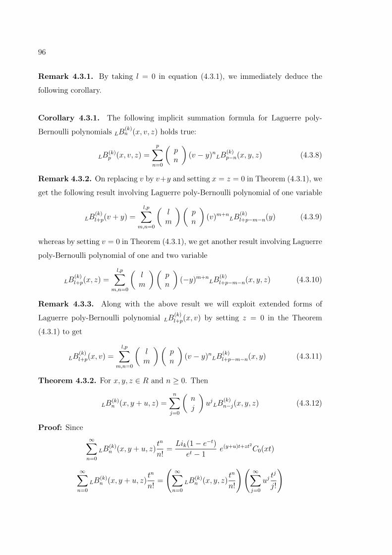
96

Remark 4.3.1. By taking l = 0 in equation (4.3.1), we immediately deduce the

following corollary.

Corollary 4.3.1. The following implicit summation formula for Laguerre poly-

Bernoulli polynomials LB(k)n (x, v, z) holds true:

LB(k)p (x, v, z) =

p∑n=0

(pn

)(v − y)nLB

(k)p−n(x, y, z) (4.3.8)

Remark 4.3.2. On replacing v by v+y and setting x = z = 0 in Theorem (4.3.1), we

get the following result involving Laguerre poly-Bernoulli polynomial of one variable

LB(k)l+p(v + y) =

l,p∑m,n=0

(lm

)(pn

)(v)m+n

LB(k)l+p−m−n(y) (4.3.9)

whereas by setting v = 0 in Theorem (4.3.1), we get another result involving Laguerre

poly-Bernoulli polynomial of one and two variable

LB(k)l+p(x, z) =

l,p∑m,n=0

(lm

)(pn

)(−y)m+n

LB(k)l+p−m−n(x, y, z) (4.3.10)

Remark 4.3.3. Along with the above result we will exploit extended forms of

Laguerre poly-Bernoulli polynomial LB(k)l+p(x, v) by setting z = 0 in the Theorem

(4.3.1) to get

LB(k)l+p(x, v) =

l,p∑m,n=0

(lm

)(pn

)(v − y)nLB

(k)l+p−m−n(x, y) (4.3.11)

Theorem 4.3.2. For x, y, z ∈ R and n ≥ 0. Then

LB(k)n (x, y + u, z) =

n∑j=0

(nj

)ujLB

(k)n−j(x, y, z) (4.3.12)

Proof: Since

∞∑n=0

LB(k)n (x, y + u, z)

tn

n!=Lik(1− e−t)

et − 1e(y+u)t+zt2C0(xt)

∞∑n=0

LB(k)n (x, y + u, z)

tn

n!=

(∞∑n=0

LB(k)n (x, y, z)

tn

n!

)(∞∑j=0

ujtj

j!

)

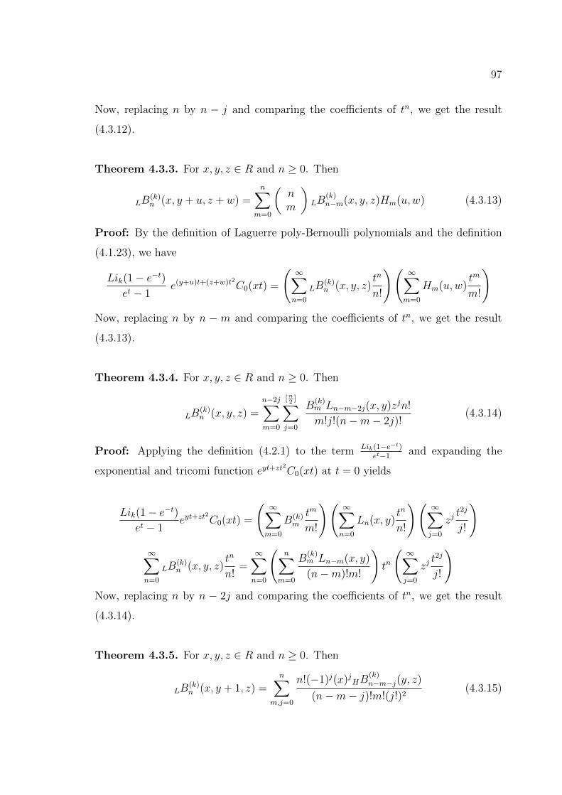
97

Now, replacing n by n − j and comparing the coefficients of tn, we get the result

(4.3.12).

Theorem 4.3.3. For x, y, z ∈ R and n ≥ 0. Then

LB(k)n (x, y + u, z + w) =

n∑m=0

(nm

)LB

(k)n−m(x, y, z)Hm(u,w) (4.3.13)

Proof: By the definition of Laguerre poly-Bernoulli polynomials and the definition

(4.1.23), we have

Lik(1− e−t)et − 1

e(y+u)t+(z+w)t2C0(xt) =

(∞∑n=0

LB(k)n (x, y, z)

tn

n!

)(∞∑m=0

Hm(u,w)tm

m!

)Now, replacing n by n − m and comparing the coefficients of tn, we get the result

(4.3.13).

Theorem 4.3.4. For x, y, z ∈ R and n ≥ 0. Then

LB(k)n (x, y, z) =

n−2j∑m=0

[n2

]∑j=0

B(k)m Ln−m−2j(x, y)zjn!

m!j!(n−m− 2j)!(4.3.14)

Proof: Applying the definition (4.2.1) to the term Lik(1−e−t)et−1

and expanding the

exponential and tricomi function eyt+zt2C0(xt) at t = 0 yields

Lik(1− e−t)et − 1

eyt+zt2

C0(xt) =

(∞∑m=0

B(k)m

tm

m!

)(∞∑n=0

Ln(x, y)tn

n!

)(∞∑j=0

zjt2j

j!

)∞∑n=0

LB(k)n (x, y, z)

tn

n!=∞∑n=0

(n∑

m=0

B(k)m Ln−m(x, y)

(n−m)!m!

)tn

(∞∑j=0

zjt2j

j!

)Now, replacing n by n − 2j and comparing the coefficients of tn, we get the result

(4.3.14).

Theorem 4.3.5. For x, y, z ∈ R and n ≥ 0. Then

LB(k)n (x, y + 1, z) =

n∑m,j=0

n!(−1)j(x)jHB(k)n−m−j(y, z)

(n−m− j)!m!(j!)2(4.3.15)

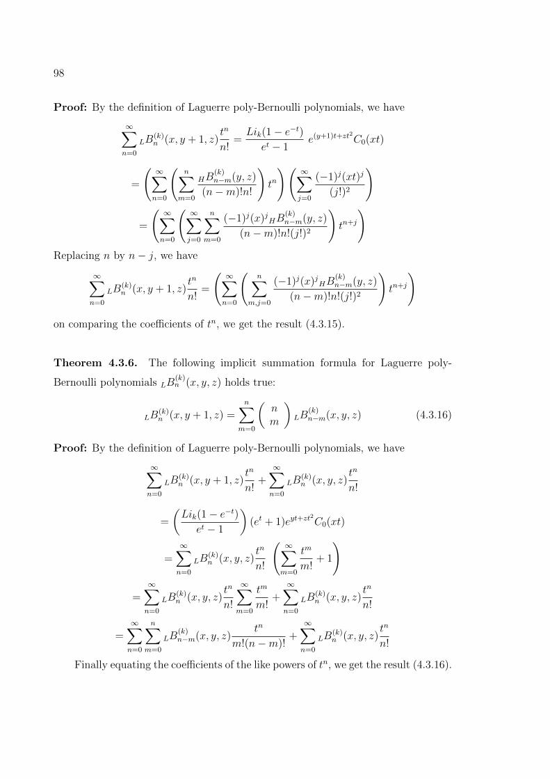
98

Proof: By the definition of Laguerre poly-Bernoulli polynomials, we have

∞∑n=0

LB(k)n (x, y + 1, z)

tn

n!=Lik(1− e−t)

et − 1e(y+1)t+zt2C0(xt)

=

(∞∑n=0

(n∑

m=0

HB(k)n−m(y, z)

(n−m)!n!

)tn

)(∞∑j=0

(−1)j(xt)j

(j!)2

)

=

(∞∑n=0

(∞∑j=0

n∑m=0

(−1)j(x)jHB(k)n−m(y, z)

(n−m)!n!(j!)2

)tn+j

)Replacing n by n− j, we have

∞∑n=0

LB(k)n (x, y + 1, z)

tn

n!=

(∞∑n=0

(n∑

m,j=0

(−1)j(x)jHB(k)n−m(y, z)

(n−m)!n!(j!)2

)tn+j

)

on comparing the coefficients of tn, we get the result (4.3.15).

Theorem 4.3.6. The following implicit summation formula for Laguerre poly-

Bernoulli polynomials LB(k)n (x, y, z) holds true:

LB(k)n (x, y + 1, z) =

n∑m=0

(nm

)LB

(k)n−m(x, y, z) (4.3.16)

Proof: By the definition of Laguerre poly-Bernoulli polynomials, we have

∞∑n=0

LB(k)n (x, y + 1, z)

tn

n!+∞∑n=0

LB(k)n (x, y, z)

tn

n!

=

(Lik(1− e−t)

et − 1

)(et + 1)eyt+zt

2

C0(xt)

=∞∑n=0

LB(k)n (x, y, z)

tn

n!

(∞∑m=0

tm

m!+ 1

)

=∞∑n=0

LB(k)n (x, y, z)

tn

n!

∞∑m=0

tm

m!+∞∑n=0

LB(k)n (x, y, z)

tn

n!

=∞∑n=0

n∑m=0

LB(k)n−m(x, y, z)

tn

m!(n−m)!+∞∑n=0

LB(k)n (x, y, z)

tn

n!

Finally equating the coefficients of the like powers of tn, we get the result (4.3.16).

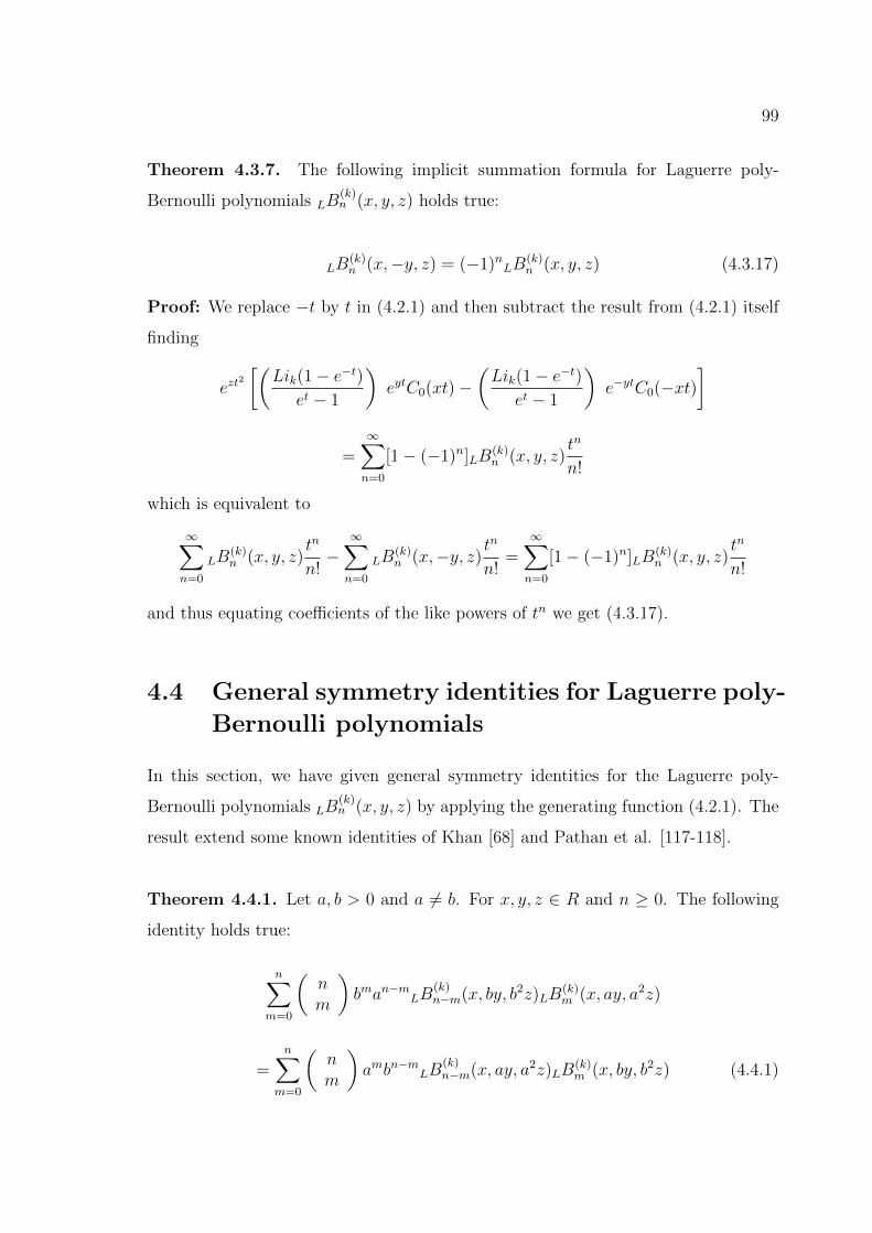
99

Theorem 4.3.7. The following implicit summation formula for Laguerre poly-

Bernoulli polynomials LB(k)n (x, y, z) holds true:

LB(k)n (x,−y, z) = (−1)nLB

(k)n (x, y, z) (4.3.17)

Proof: We replace −t by t in (4.2.1) and then subtract the result from (4.2.1) itself

finding

ezt2

[(Lik(1− e−t)

et − 1

)eytC0(xt)−

(Lik(1− e−t)

et − 1

)e−ytC0(−xt)

]

=∞∑n=0

[1− (−1)n]LB(k)n (x, y, z)

tn

n!

which is equivalent to

∞∑n=0

LB(k)n (x, y, z)

tn

n!−∞∑n=0

LB(k)n (x,−y, z) t

n

n!=∞∑n=0

[1− (−1)n]LB(k)n (x, y, z)

tn

n!

and thus equating coefficients of the like powers of tn we get (4.3.17).

4.4 General symmetry identities for Laguerre poly-

Bernoulli polynomials

In this section, we have given general symmetry identities for the Laguerre poly-

Bernoulli polynomials LB(k)n (x, y, z) by applying the generating function (4.2.1). The

result extend some known identities of Khan [68] and Pathan et al. [117-118].

Theorem 4.4.1. Let a, b > 0 and a 6= b. For x, y, z ∈ R and n ≥ 0. The following

identity holds true:

n∑m=0

(nm

)bman−mLB

(k)n−m(x, by, b2z)LB

(k)m (x, ay, a2z)

=n∑

m=0

(nm

)ambn−mLB

(k)n−m(x, ay, a2z)LB

(k)m (x, by, b2z) (4.4.1)

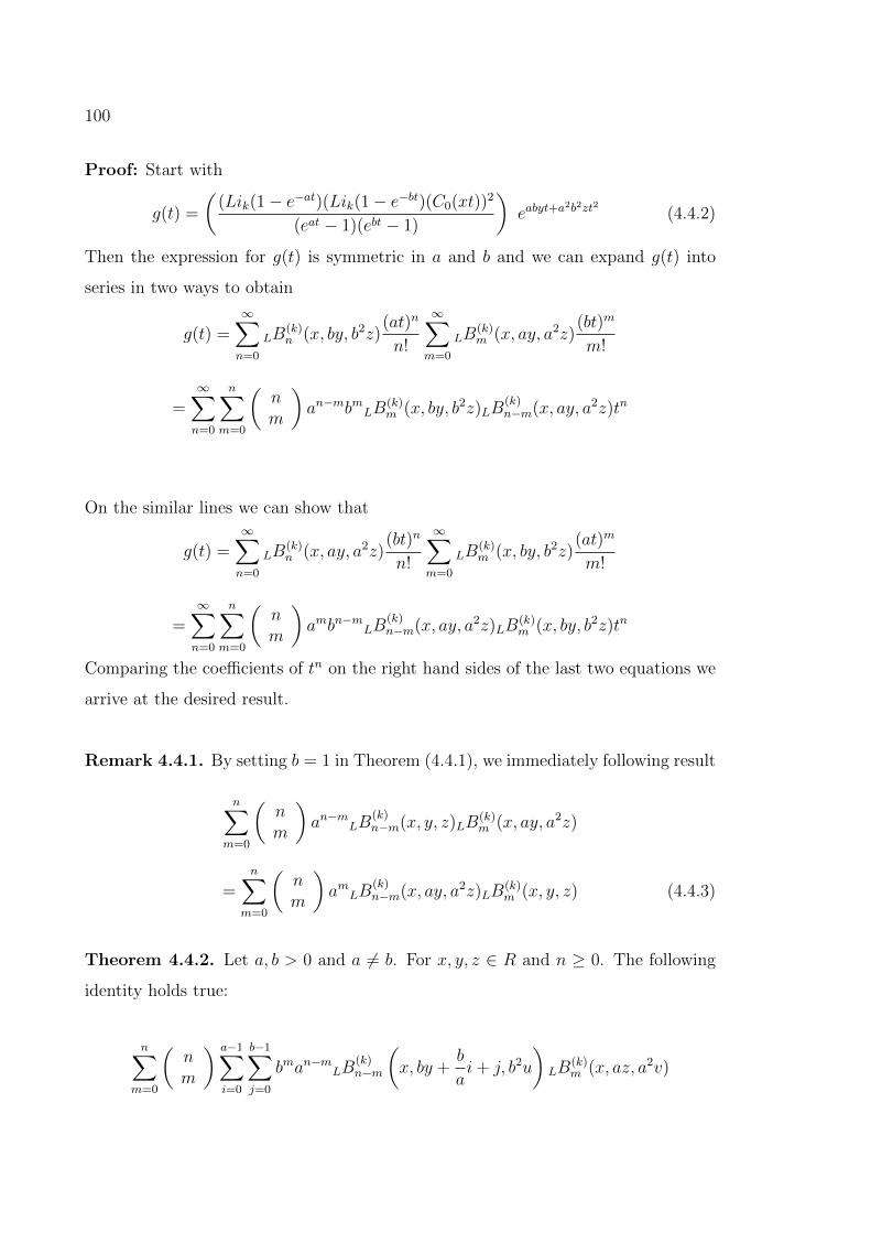
100

Proof: Start with

g(t) =

((Lik(1− e−at)(Lik(1− e−bt)(C0(xt))2

(eat − 1)(ebt − 1)

)eabyt+a

2b2zt2 (4.4.2)

Then the expression for g(t) is symmetric in a and b and we can expand g(t) into

series in two ways to obtain

g(t) =∞∑n=0

LB(k)n (x, by, b2z)

(at)n

n!

∞∑m=0

LB(k)m (x, ay, a2z)

(bt)m

m!

=∞∑n=0

n∑m=0

(nm

)an−mbmLB

(k)m (x, by, b2z)LB

(k)n−m(x, ay, a2z)tn

On the similar lines we can show that

g(t) =∞∑n=0

LB(k)n (x, ay, a2z)

(bt)n

n!

∞∑m=0

LB(k)m (x, by, b2z)

(at)m

m!

=∞∑n=0

n∑m=0

(nm

)ambn−mLB

(k)n−m(x, ay, a2z)LB

(k)m (x, by, b2z)tn

Comparing the coefficients of tn on the right hand sides of the last two equations we

arrive at the desired result.

Remark 4.4.1. By setting b = 1 in Theorem (4.4.1), we immediately following result

n∑m=0

(nm

)an−mLB

(k)n−m(x, y, z)LB

(k)m (x, ay, a2z)

=n∑

m=0

(nm

)amLB

(k)n−m(x, ay, a2z)LB

(k)m (x, y, z) (4.4.3)

Theorem 4.4.2. Let a, b > 0 and a 6= b. For x, y, z ∈ R and n ≥ 0. The following

identity holds true:

n∑m=0

(nm

) a−1∑i=0

b−1∑j=0

bman−mLB(k)n−m

(x, by +

b

ai+ j, b2u

)LB

(k)m (x, az, a2v)

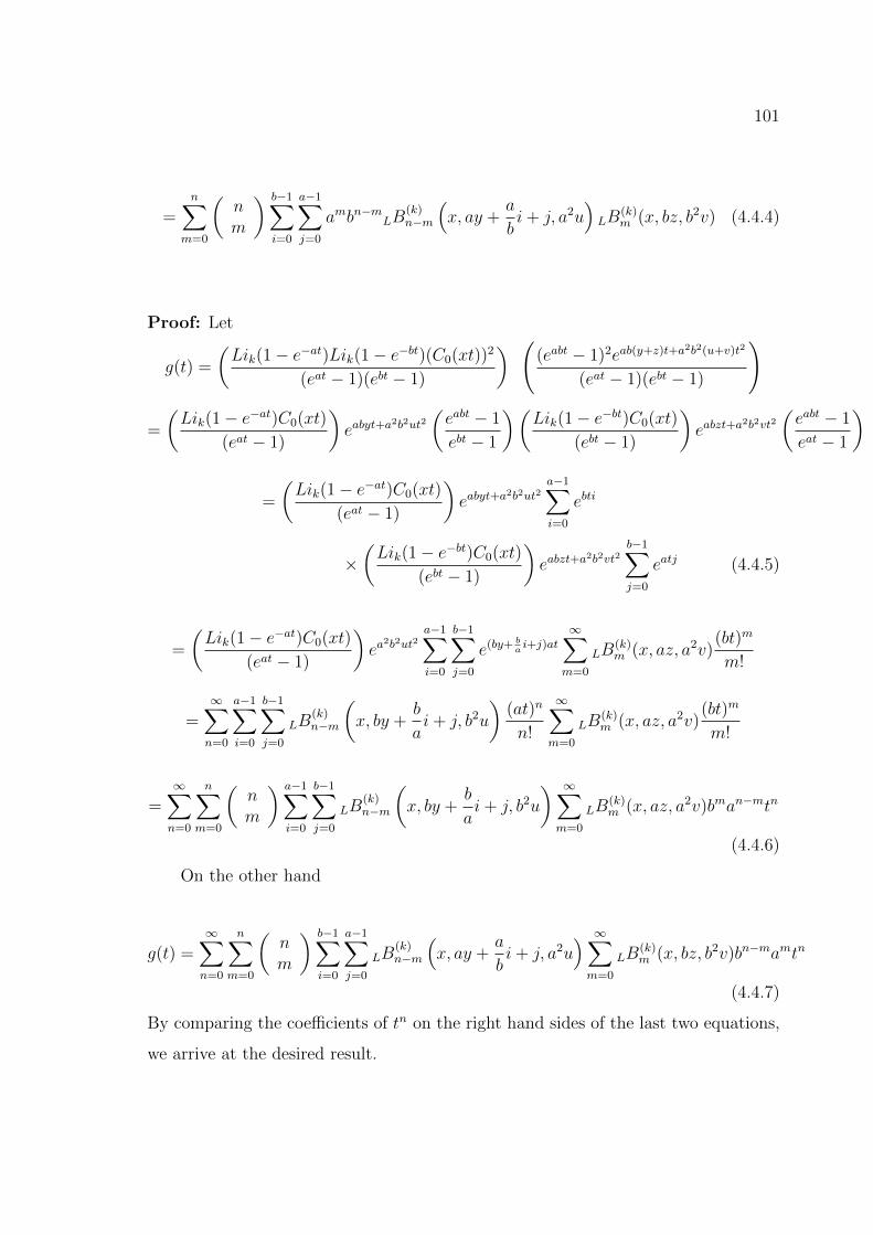
101

=n∑

m=0

(nm

) b−1∑i=0

a−1∑j=0

ambn−mLB(k)n−m

(x, ay +

a

bi+ j, a2u

)LB

(k)m (x, bz, b2v) (4.4.4)

Proof: Let

g(t) =

(Lik(1− e−at)Lik(1− e−bt)(C0(xt))2

(eat − 1)(ebt − 1)

) ((eabt − 1)2eab(y+z)t+a2b2(u+v)t2

(eat − 1)(ebt − 1)

)

=

(Lik(1− e−at)C0(xt)

(eat − 1)

)eabyt+a

2b2ut2(eabt − 1

ebt − 1

)(Lik(1− e−bt)C0(xt)

(ebt − 1)

)eabzt+a

2b2vt2(eabt − 1

eat − 1

)

=

(Lik(1− e−at)C0(xt)

(eat − 1)

)eabyt+a

2b2ut2a−1∑i=0

ebti

×(Lik(1− e−bt)C0(xt)

(ebt − 1)

)eabzt+a

2b2vt2b−1∑j=0

eatj (4.4.5)

=

(Lik(1− e−at)C0(xt)

(eat − 1)

)ea

2b2ut2a−1∑i=0

b−1∑j=0

e(by+ bai+j)at

∞∑m=0

LB(k)m (x, az, a2v)

(bt)m

m!

=∞∑n=0

a−1∑i=0

b−1∑j=0

LB(k)n−m

(x, by +

b

ai+ j, b2u

)(at)n

n!

∞∑m=0

LB(k)m (x, az, a2v)

(bt)m

m!

=∞∑n=0

n∑m=0

(nm

) a−1∑i=0

b−1∑j=0

LB(k)n−m

(x, by +

b

ai+ j, b2u

) ∞∑m=0

LB(k)m (x, az, a2v)bman−mtn

(4.4.6)

On the other hand

g(t) =∞∑n=0

n∑m=0

(nm

) b−1∑i=0

a−1∑j=0

LB(k)n−m

(x, ay +

a

bi+ j, a2u

) ∞∑m=0

LB(k)m (x, bz, b2v)bn−mamtn

(4.4.7)

By comparing the coefficients of tn on the right hand sides of the last two equations,

we arrive at the desired result.

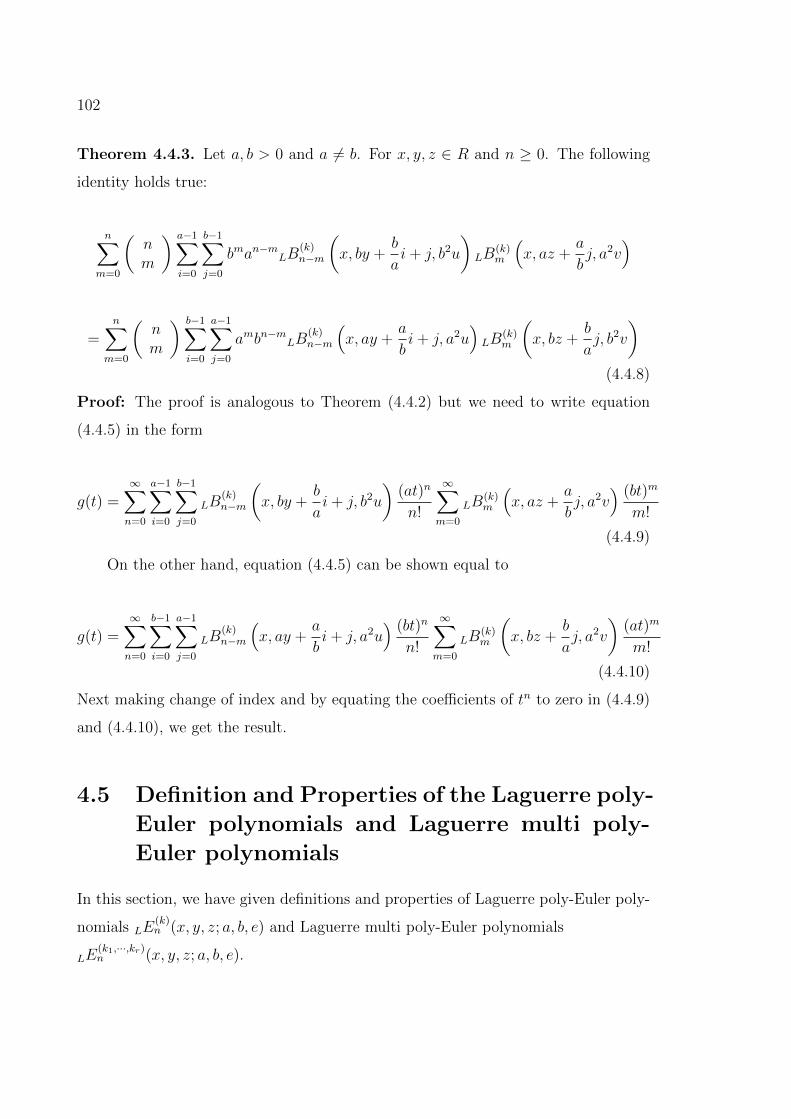
102

Theorem 4.4.3. Let a, b > 0 and a 6= b. For x, y, z ∈ R and n ≥ 0. The following

identity holds true:

n∑m=0

(nm

) a−1∑i=0

b−1∑j=0

bman−mLB(k)n−m

(x, by +

b

ai+ j, b2u

)LB

(k)m

(x, az +

a

bj, a2v

)

=n∑

m=0

(nm

) b−1∑i=0

a−1∑j=0

ambn−mLB(k)n−m

(x, ay +

a

bi+ j, a2u

)LB

(k)m

(x, bz +

b

aj, b2v

)(4.4.8)

Proof: The proof is analogous to Theorem (4.4.2) but we need to write equation

(4.4.5) in the form

g(t) =∞∑n=0

a−1∑i=0

b−1∑j=0

LB(k)n−m

(x, by +

b

ai+ j, b2u

)(at)n

n!

∞∑m=0

LB(k)m

(x, az +

a

bj, a2v

) (bt)m

m!

(4.4.9)

On the other hand, equation (4.4.5) can be shown equal to

g(t) =∞∑n=0

b−1∑i=0

a−1∑j=0

LB(k)n−m

(x, ay +

a

bi+ j, a2u

) (bt)n

n!

∞∑m=0

LB(k)m

(x, bz +

b

aj, a2v

)(at)m

m!

(4.4.10)

Next making change of index and by equating the coefficients of tn to zero in (4.4.9)

and (4.4.10), we get the result.

4.5 Definition and Properties of the Laguerre poly-

Euler polynomials and Laguerre multi poly-

Euler polynomials

In this section, we have given definitions and properties of Laguerre poly-Euler poly-

nomials LE(k)n (x, y, z; a, b, e) and Laguerre multi poly-Euler polynomials

LE(k1,···,kr)n (x, y, z; a, b, e).

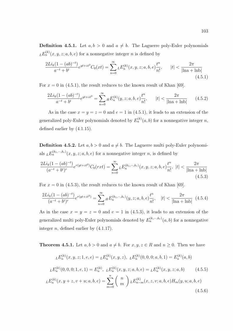
103

Definition 4.5.1. Let a, b > 0 and a 6= b. The Laguerre poly-Euler polynomials

LE(k)n (x, y, z; a, b, e) for a nonnegative integer n is defined by

2Lik(1− (ab)−t)

a−t + bteyt+zt

2

C0(xt) =∞∑n=0

LE(k)n (x, y, z; a, b, e)

tn

n!, |t| < 2π

|lna + lnb|(4.5.1)

For x = 0 in (4.5.1), the result reduces to the known result of Khan [69].

2Lik(1− (ab)−t)

a−t + bteyt+zt

2

=∞∑n=0

HE(k)n (y, z; a, b, e)

tn

n!, |t| < 2π

|lna + lnb|(4.5.2)

As in the case x = y = z = 0 and e = 1 in (4.5.1), it leads to an extension of the

generalized poly-Euler polynomials denoted by E(k)n (a, b) for a nonnegative integer n,

defined earlier by (4.1.15).

Definition 4.5.2. Let a, b > 0 and a 6= b. The Laguerre multi poly-Euler polynomi-

als LE(k1,···,kr)n (x, y, z; a, b, e) for a nonnegative integer n, is defined by

2Lik(1− (ab)−t)

(a−t + bt)rer(yt+zt

2)C0(rxt) =∞∑n=0

LE(k1,···,kr)n (x, y, z; a, b, e)

tn

n!, |t| < 2π

|lna + lnb|(4.5.3)

For x = 0 in (4.5.3), the result reduces to the known result of Khan [69].

2Lik(1− (ab)−t)

(a−t + bt)rer(yt+zt

2) =∞∑n=0

HE(k1,···,kr)n (y, z; a, b, e)

tn

n!, |t| < 2π

|lna + lnb|(4.5.4)

As in the case x = y = z = 0 and e = 1 in (4.5.3), it leads to an extension of the

generalized multi poly-Euler polynomials denoted by E(k,···,kr)n (a, b) for a nonnegative

integer n, defined earlier by (4.1.17).

Theorem 4.5.1. Let a, b > 0 and a 6= b. For x, y, z ∈ R and n ≥ 0. Then we have

LE(k)n (x, y, z; 1, e, e) = LE

(k)n (x, y, z), LE

(k)n (0, 0, 0; a, b, 1) = E(k)

n (a, b)

LE(k)n (0, 0, 0; 1, e, 1) = E(k)

n , LE(k)n (x, y, z; a, b, e) = LE

(k)n (x, y, z; a, b) (4.5.5)

LE(k)n (x, y + z, v + u; a, b, e) =

n∑m=0

(nm

)LE

(k)n−m(x, z, v; a, b, e)Hm(y, u; a, b, e)

(4.5.6)

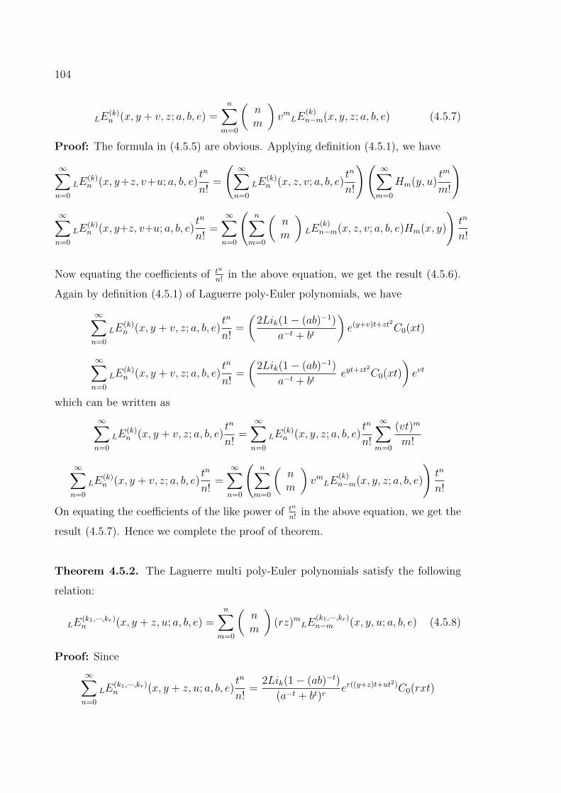
104

LE(k)n (x, y + v, z; a, b, e) =

n∑m=0

(nm

)vmLE

(k)n−m(x, y, z; a, b, e) (4.5.7)

Proof: The formula in (4.5.5) are obvious. Applying definition (4.5.1), we have

∞∑n=0

LE(k)n (x, y+z, v+u; a, b, e)

tn

n!=

(∞∑n=0

LE(k)n (x, z, v; a, b, e)

tn

n!

)(∞∑m=0

Hm(y, u)tm

m!

)∞∑n=0

LE(k)n (x, y+z, v+u; a, b, e)

tn

n!=∞∑n=0

(n∑

m=0

(nm

)LE

(k)n−m(x, z, v; a, b, e)Hm(x, y)

)tn

n!

Now equating the coefficients of tn

n!in the above equation, we get the result (4.5.6).

Again by definition (4.5.1) of Laguerre poly-Euler polynomials, we have

∞∑n=0

LE(k)n (x, y + v, z; a, b, e)

tn

n!=

(2Lik(1− (ab)−1)

a−t + bt

)e(y+v)t+zt2C0(xt)

∞∑n=0

LE(k)n (x, y + v, z; a, b, e)

tn

n!=

(2Lik(1− (ab)−1)

a−t + bteyt+zt

2

C0(xt)

)evt

which can be written as

∞∑n=0

LE(k)n (x, y + v, z; a, b, e)

tn

n!=∞∑n=0

LE(k)n (x, y, z; a, b, e)

tn

n!

∞∑m=0

(vt)m

m!

∞∑n=0

LE(k)n (x, y + v, z; a, b, e)

tn

n!=∞∑n=0

(n∑

m=0

(nm

)vmLE

(k)n−m(x, y, z; a, b, e)

)tn

n!

On equating the coefficients of the like power of tn

n!in the above equation, we get the

result (4.5.7). Hence we complete the proof of theorem.

Theorem 4.5.2. The Laguerre multi poly-Euler polynomials satisfy the following

relation:

LE(k1,···,kr)n (x, y + z, u; a, b, e) =

n∑m=0

(nm

)(rz)mLE

(k1,···,kr)n−m (x, y, u; a, b, e) (4.5.8)

Proof: Since

∞∑n=0

LE(k1,···,kr)n (x, y + z, u; a, b, e)

tn

n!=

2Lik(1− (ab)−t)

(a−t + bt)rer((y+z)t+ut2)C0(rxt)

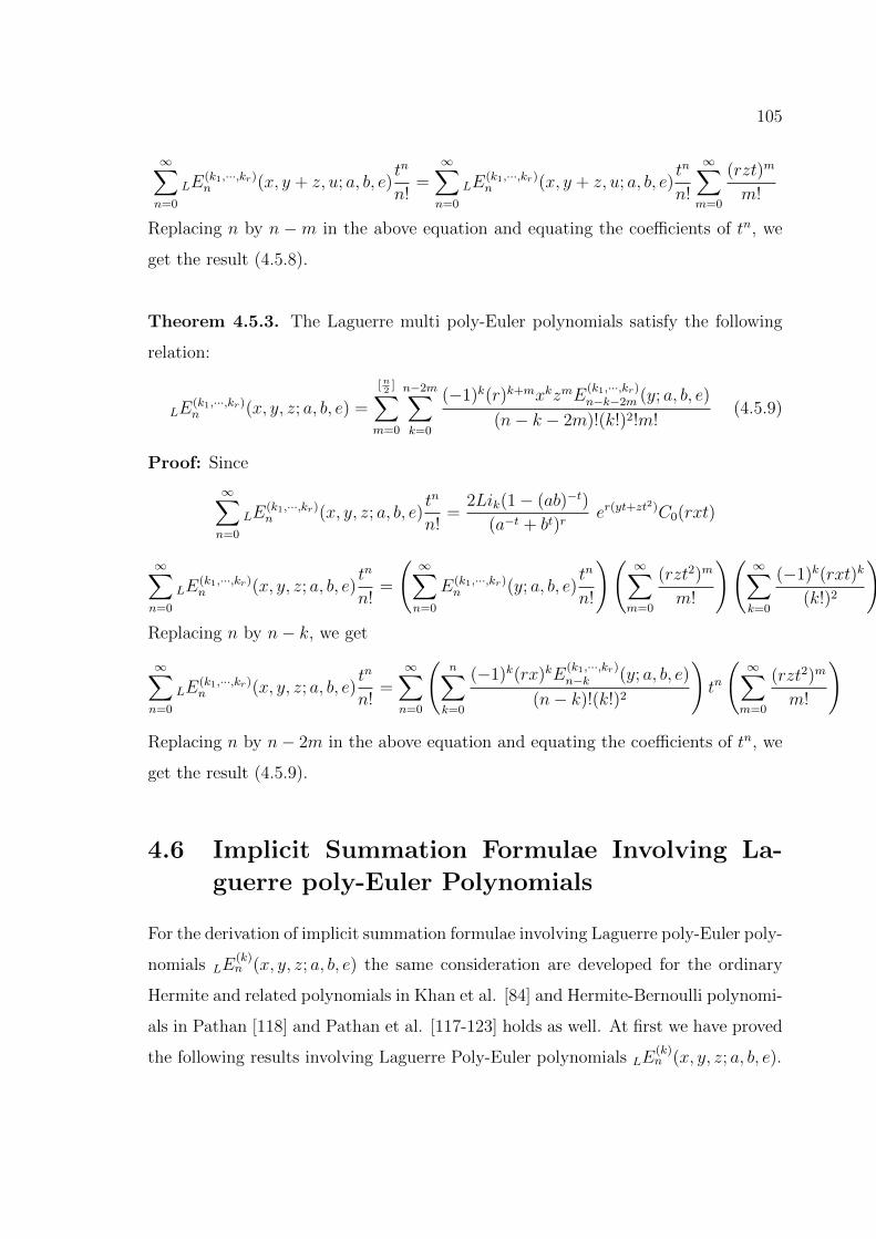
105

∞∑n=0

LE(k1,···,kr)n (x, y + z, u; a, b, e)

tn

n!=∞∑n=0

LE(k1,···,kr)n (x, y + z, u; a, b, e)

tn

n!

∞∑m=0

(rzt)m

m!

Replacing n by n −m in the above equation and equating the coefficients of tn, we

get the result (4.5.8).

Theorem 4.5.3. The Laguerre multi poly-Euler polynomials satisfy the following

relation:

LE(k1,···,kr)n (x, y, z; a, b, e) =

[n2

]∑m=0

n−2m∑k=0

(−1)k(r)k+mxkzmE(k1,···,kr)n−k−2m (y; a, b, e)

(n− k − 2m)!(k!)2!m!(4.5.9)

Proof: Since

∞∑n=0

LE(k1,···,kr)n (x, y, z; a, b, e)

tn

n!=

2Lik(1− (ab)−t)

(a−t + bt)rer(yt+zt

2)C0(rxt)

∞∑n=0

LE(k1,···,kr)n (x, y, z; a, b, e)

tn

n!=

(∞∑n=0

E(k1,···,kr)n (y; a, b, e)

tn

n!

)(∞∑m=0

(rzt2)m

m!

)(∞∑k=0

(−1)k(rxt)k

(k!)2

)Replacing n by n− k, we get

∞∑n=0

LE(k1,···,kr)n (x, y, z; a, b, e)

tn

n!=∞∑n=0

(n∑k=0

(−1)k(rx)kE(k1,···,kr)n−k (y; a, b, e)

(n− k)!(k!)2

)tn

(∞∑m=0

(rzt2)m

m!

)

Replacing n by n− 2m in the above equation and equating the coefficients of tn, we

get the result (4.5.9).

4.6 Implicit Summation Formulae Involving La-

guerre poly-Euler Polynomials

For the derivation of implicit summation formulae involving Laguerre poly-Euler poly-

nomials LE(k)n (x, y, z; a, b, e) the same consideration are developed for the ordinary

Hermite and related polynomials in Khan et al. [84] and Hermite-Bernoulli polynomi-

als in Pathan [118] and Pathan et al. [117-123] holds as well. At first we have proved

the following results involving Laguerre Poly-Euler polynomials LE(k)n (x, y, z; a, b, e).

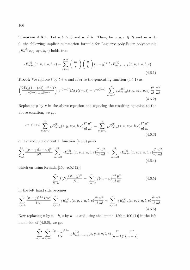
106

Theorem 4.6.1. Let a, b > 0 and a 6= b. Then, for x, y, z ∈ R and m,n ≥

0, the following implicit summation formula for Laguerre poly-Euler polynomials

LE(k)n (x, y, z; a, b, e) holds true:

LE(k)m+n(x, v, z; a, b, e) =

m,n∑s,k=0

(ms

)(nk

)(v − y)s+kLE

(k)m+n−s−k(x, y, z; a, b, e)

(4.6.1)

Proof: We replace t by t+ u and rewrite the generating function (4.5.1) as(2Lik(1− (ab)−(t+u))

a−(t+u) + b(t+u)

)ez(t+u)2C0(x(t+u)) = e−y(t+u)

∞∑m,n=0

LE(k)m+n(x, y, z; a, b, e)

tn

n!

um

m!

(4.6.2)

Replacing y by v in the above equation and equating the resulting equation to the

above equation, we get

e(v−y)(t+u)

∞∑m,n=0

LE(k)m+n(x, y, z; a, b, e)

tn

n!

um

m!=

∞∑m,n=0

LE(k)m+n(x, v, z; a, b, e)

tn

n!

um

m!

(4.6.3)

on expanding exponential function (4.6.3) gives

∞∑N=0

[(v − y)(t+ u)]N

N !

∞∑m,n=0

LE(k)m+n(x, y, z; a, b, e)

tn

n!

um

m!=

∞∑m,n=0

LE(k)m+n(x, v, z; a, b, e)

tn

n!

um

m!

(4.6.4)

which on using formula [150; p.52 (2)]

∞∑N=0

f(N)(x+ y)N

N !=

∞∑n,m=0

f(m+ n)xn

n!

ym

m!(4.6.5)

in the left hand side becomes

∞∑k,s=0

(v − y)k+s tkus

k!s!

∞∑m,n=0

LE(k)m+n(x, y, z; a, b, e)

tn

n!

um

m!=

∞∑m,n=0

LE(k)m+n(x, v, z; a, b, e)

tn

n!

um

m!

(4.6.6)

Now replacing n by n− k, s by n− s and using the lemma [150; p.100 (1)] in the left

hand side of (4.6.6), we get

∞∑m,n=0

∞∑k,s=0

(v − y)k+s

k!s!LE

(k)m+n−k−s(x, y, z; a, b, e)

tn

(n− k)!

um

(m− s)!

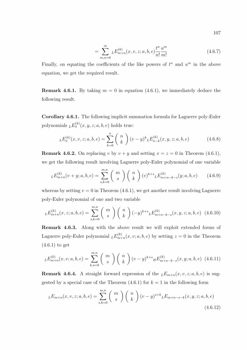
107

=∞∑

m,n=0

LE(k)m+n(x, v, z; a, b, e)

tn

n!

um

m!(4.6.7)

Finally, on equating the coefficients of the like powers of tn and um in the above

equation, we get the required result.

Remark 4.6.1. By taking m = 0 in equation (4.6.1), we immediately deduce the

following result.

Corollary 4.6.1. The following implicit summation formula for Laguerre poly-Euler

polynomials LE(k)n (x, y, z; a, b, e) holds true:

LE(k)n (x, v, z; a, b, e) =

n∑k=0

(nk

)(v − y)kLE

(k)n−k(x, y, z; a, b, e) (4.6.8)

Remark 4.6.2. On replacing v by v + y and setting x = z = 0 in Theorem (4.6.1),

we get the following result involving Laguerre poly-Euler polynomial of one variable

LE(k)m+n(v + y; a, b, e) =

m,n∑s,k=0

(ms

)(nk

)(v)k+s

LE(k)m+n−k−s(y; a, b, e) (4.6.9)

whereas by setting v = 0 in Theorem (4.6.1), we get another result involving Laguerre

poly-Euler polynomial of one and two variable

LE(k)m+n(x, z; a, b, e) =

m,n∑s,k=0

(ms

)(nk

)(−y)k+s

LE(k)m+n−k−s(x, y, z; a, b, e) (4.6.10)

Remark 4.6.3. Along with the above result we will exploit extended forms of

Laguerre poly-Euler polynomial LE(k)m+n(x, v; a, b, e) by setting z = 0 in the Theorem

(4.6.1) to get

LE(k)m+n(x, v; a, b, e) =

m,n∑k,s=0

(ms

)(nk

)(v − y)k+s

HE(k)m+n−k−s(x, y; a, b, e) (4.6.11)

Remark 4.6.4. A straight forward expression of the LEm+n(x, v, z; a, b, e) is sug-

gested by a special case of the Theorem (4.6.1) for k = 1 in the following form

LEm+n(x, v, z; a, b, e) =

m,n∑s,k=0

(ms

)(nk

)(v − y)s+kLEm+n−s−k(x, y, z; a, b, e)

(4.6.12)

108

Theorem 4.6.2. Let a, b > 0 and a 6= b. Then, for x, y, z ∈ R and m,n ≥

0, the following implicit summation formula for Laguerre poly-Euler polynomials

LE(k)n (x, y, z; a, b, e) holds true:

LE(k)n (x, y + u, z; a, b, e) =

n∑j=0

(nj

)ujLE

(k)n−j(x, y, z; a, b, e) (4.6.13)

Proof: Since

∞∑n=0

LE(k)n (x, y + u, z; a, b, e)

tn

n!=

2Lik(1− (ab)−t)

a−t + bte(y+u)t+zt2C0(xt)

∞∑n=0

LE(k)n (x, y + u, z; a, b, e)

tn

n!=

(∞∑n=0

LE(k)n (x, y, z; a, b, e)

tn

n!

)(∞∑j=0

ujtj

j!

)Now, replacing n by n − j and comparing the coefficients of tn, we get the result

(4.6.13).

Theorem 4.6.3. Let a, b > 0 and a 6= b. Then, for x, y, z ∈ R and m,n ≥

0, the following implicit summation formula for Laguerre poly-Euler polynomials

LE(k)n (x, y, z; a, b, e) holds true:

LE(k)n (x, y + u, z + w; a, b, e) =

n∑m=0

(nm

)LE

(k)n−m(x, y, z; a, b, e)Hm(u,w) (4.6.14)

Proof: By the definition of Laguerre poly-Euler polynomials and the definition

(4.1.23), we have(2Lik(1− (ab)−t)

a−t + bt

)e(y+u)t+(z+w)t2C0(xt) =

(∞∑n=0

LE(k)n (x, y, z)

tn

n!

)(∞∑m=0

Hm(u,w)tm

m!

)

Now, replacing n by n − m and comparing the coefficients of tn, we get the result

(4.6.14).

Theorem 4.6.4. Let a, b > 0 and a 6= b. Then, for x, y, z ∈ R and m,n ≥

0, the following implicit summation formula for Laguerre poly-Euler polynomials

LE(k)n (x, y, z; a, b, e) holds true:

109

LE(k)n (x, y, z; a, b, e) =

n−2j∑m=0

[n2

]∑j=0

E(k)m (a, b)Ln−m−2j(x, y)zjn!

m!j!(n−m− 2j)!(4.6.15)

Proof: Applying the definition (4.5.1) to the term(

2Lik(1−(ab)−t)a−t+bt

)and expanding the

exponential and tricomi function eyt+zt2C0(xt) at t = 0 yields

(2Lik(1− (ab)−t)

a−t + bt

)eyt+zt

2

C0(xt) =

(∞∑m=0

E(k)m (a, b)

tm

m!

)(∞∑n=0

Ln(x, y)tn

n!

)(∞∑j=0

zj(t)2j

j!

)

∞∑n=0

LE(k)n (x, y, z; a, b, e)

tn

n!=∞∑n=0

(n∑

m=0

E(k)m (a, b)Ln−m(x, y)

)tn

n!

(∞∑j=0

zjt2j

j!

)Now, replacing n by n − 2j and comparing the coefficients of tn, we get the result

(4.6.15).

Theorem 4.6.5. Let a, b > 0 and a 6= b. Then, for x, y, z ∈ R and m,n ≥

0, the following implicit summation formula for Laguerre poly-Euler polynomials

LE(k)n (x, y, z; a, b, e) holds true:

LE(k)n (x, y + 1, z; a, b, e) =

n∑m,j=0

n!(−1)j(x)jHE(k)n−m−j(y, z; a, b, e)

(n−m− j)!m!(j!)2(4.6.16)

Proof: By the definition of Laguerre poly-Euler polynomials, we have

∞∑n=0

LE(k)n (x, y + 1, z; a, b, e)

tn

n!=

(2Lik(1− (ab)−t)

a−t + bt

)e(y+1)t+zt2C0(xt)

=

(∞∑n=0

(n∑

m=0

HE(k)n−m(y, z; a, b, e)

(n−m)!n!

)tn

)(∞∑j=0

(−1)j(xt)j

(j!)2

)

=

(∞∑n=0

(∞∑j=0

n∑m=0

(−1)j(x)jHE(k)n−m(y, z; a, b, e)

(n−m)!n!(j!)2

)tn+j

)Replacing n by n− j, we have

∞∑n=0

LE(k)n (x, y + 1, z; a, b, e)

tn

n!=

(∞∑n=0

(n∑

m,j=0

(−1)j(x)jHE(k)n−m(y, z; a, b, e)

(n−m)!n!(j!)2

)tn+j

)

110

On comparing the coefficients of tn, we get the result (4.6.16).

Theorem 4.6.6. Let a, b > 0 and a 6= b. Then, for x, y, z ∈ R and m,n ≥

0, the following implicit summation formula for Laguerre poly-Euler polynomials

LE(k)n (x, y, z; a, b, e) holds true:

LE(k)n (x, y + 1, z; a, b, e) =

n∑m=0

(nm

)LE

(k)n−m(x, y, z; a, b, e) (4.6.17)

Proof: By the definition of Laguerre poly-Euler polynomials, we have

∞∑n=0

LE(k)n (x, y + 1, z; a, b, e)

tn

n!−∞∑n=0

LE(k)n (x, y, z; a, b, e)

tn

n!

=

(2Lik(1− (ab)−t)

a−t + bt

)(et − 1)eyt+zt

2

C0(xt)

=∞∑n=0

LE(k)n (x, y, z; a, b, e)

tn

n!

(∞∑m=0

tm

m!− 1

)

=∞∑n=0

LE(k)n (x, y, z; a, b, e)

tn

n!

∞∑m=0

tm

m!−∞∑n=0

LE(k)n (x, y, z; a, b, e)

tn

n!

=∞∑n=0

n∑m=0

LE(k)n−m(x, y, z; a, b, e)

tn

m!(n−m)!−∞∑n=0

LE(k)n (x, y, z; a, b, e)

tn

n!

Finally equating the coefficients of the like powers of tn in the above equation, we get

the result (4.6.17).

Theorem 4.6.7. Let a, b > 0 and a 6= b. Then, for x, y, z ∈ R and m,n ≥

0, the following implicit summation formula for Laguerre poly-Euler polynomials

LE(k)n (x, y, z; a, b, e) holds true:

LE(k)n−m(x,−y, z; a, b, e) = (−1)nLE

(k)n (x, y, z; a, b, e) (4.6.18)

Proof: We replace −t by t in (2.1) and then subtract the result from (2.1) itself

finding

ezt2

[(2Lik(1− (ab)−t)

a−t + bt

)(eyt − (ab)αte−yt)(C0(xt)− C0(−xt))

]

111

=∞∑n=0

[1− (−1)n]LE(k)n (x, y, z; a, b, e)

tn

n!

which is equivalent to

=∞∑n=0

LE(k)n (x, y, z; a, b, e)

tn

n!−∞∑n=0

LE(k)n (x,−y, z; a, b, e) t

n

n!

=∞∑n=0

LE(k)n (x, y, z; a, b, e)

tn

n!− LE

(k)n (x,−y, z; a, b, e) tn

(n−m)!

=∞∑n=0

[1− (−1)n]LE(k)n (x, y, z; a, b, e)

tn

n!

and thus equating coefficients of the like powers of tn in the above equation, we get

(4.6.18).

4.7 General Symmetry Identities for Laguerre poly-

Euler Polynomials

In this section, we have derived general symmetry identities for the Laguerre poly-

Euler polynomials LE(k)n (x, y, z; a, b, e) by applying the generating function (4.5.1). It

turns out some known identities of Khan [67-69], Pathan et al. [117-123], Yang et al.

[183], Zhang et al. [184].

Theorem 4.7.1. Let a, b > 0 and a 6= b. Then, for x, y, z ∈ R and m,n ≥ 0. The

following identity holds true:

n∑m=0

(nm

)bman−mEG

(k)n−m(x, by, b2z; b, e)LE

(k)m (x, ay, a2z; a, e)

=n∑

m=0

(nm

)ambn−mLE

(k)n−m(x, ay, a2z; a, e)LE

(k)m (x, by, b2z; b, e) (4.7.1)

Proof: Start with

g(t) =

((2Lik(1− (ab)−t)C0(xt))2

(a−at + bat)(a−bt + bbt)

)eabyt+a

2b2zt2 (4.7.2)

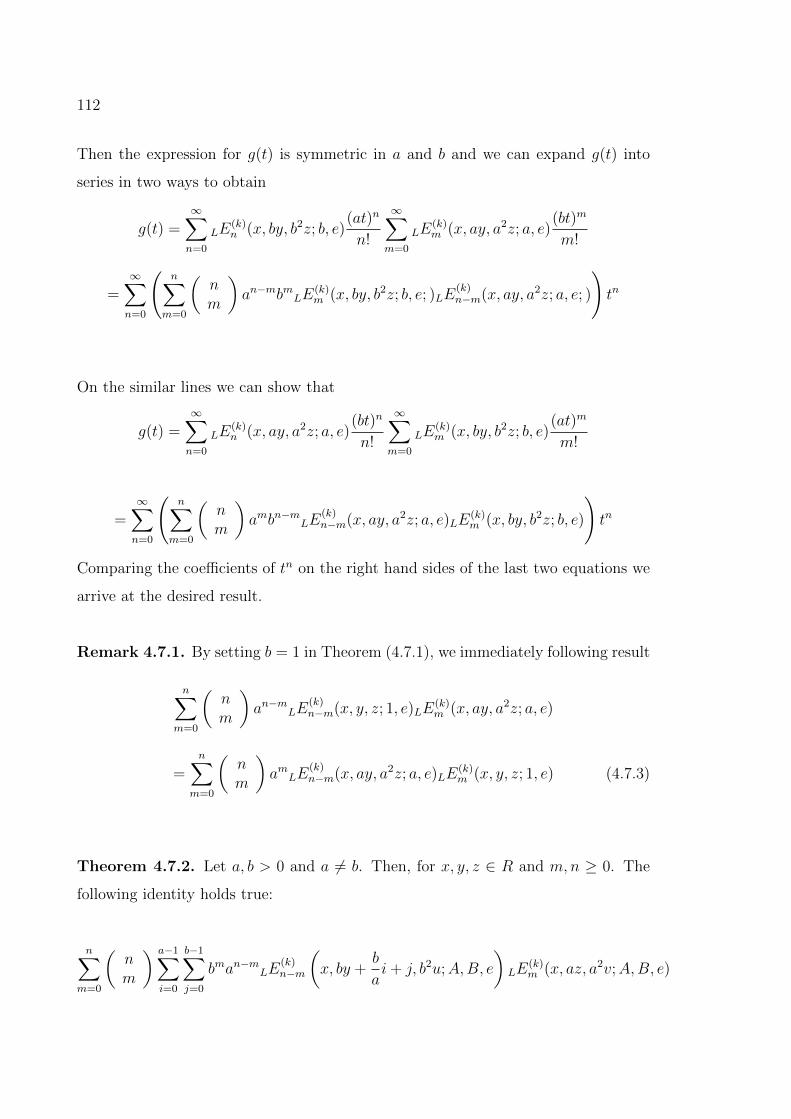
112

Then the expression for g(t) is symmetric in a and b and we can expand g(t) into

series in two ways to obtain

g(t) =∞∑n=0

LE(k)n (x, by, b2z; b, e)

(at)n

n!

∞∑m=0

LE(k)m (x, ay, a2z; a, e)

(bt)m

m!

=∞∑n=0

(n∑

m=0

(nm

)an−mbmLE

(k)m (x, by, b2z; b, e; )LE

(k)n−m(x, ay, a2z; a, e; )

)tn

On the similar lines we can show that

g(t) =∞∑n=0

LE(k)n (x, ay, a2z; a, e)

(bt)n

n!

∞∑m=0

LE(k)m (x, by, b2z; b, e)

(at)m

m!

=∞∑n=0

(n∑

m=0

(nm

)ambn−mLE

(k)n−m(x, ay, a2z; a, e)LE

(k)m (x, by, b2z; b, e)

)tn

Comparing the coefficients of tn on the right hand sides of the last two equations we

arrive at the desired result.

Remark 4.7.1. By setting b = 1 in Theorem (4.7.1), we immediately following result

n∑m=0

(nm

)an−mLE

(k)n−m(x, y, z; 1, e)LE

(k)m (x, ay, a2z; a, e)

=n∑

m=0

(nm

)amLE

(k)n−m(x, ay, a2z; a, e)LE

(k)m (x, y, z; 1, e) (4.7.3)

Theorem 4.7.2. Let a, b > 0 and a 6= b. Then, for x, y, z ∈ R and m,n ≥ 0. The

following identity holds true:

n∑m=0

(nm

) a−1∑i=0

b−1∑j=0

bman−mLE(k)n−m

(x, by +

b

ai+ j, b2u;A,B, e

)LE

(k)m (x, az, a2v;A,B, e)

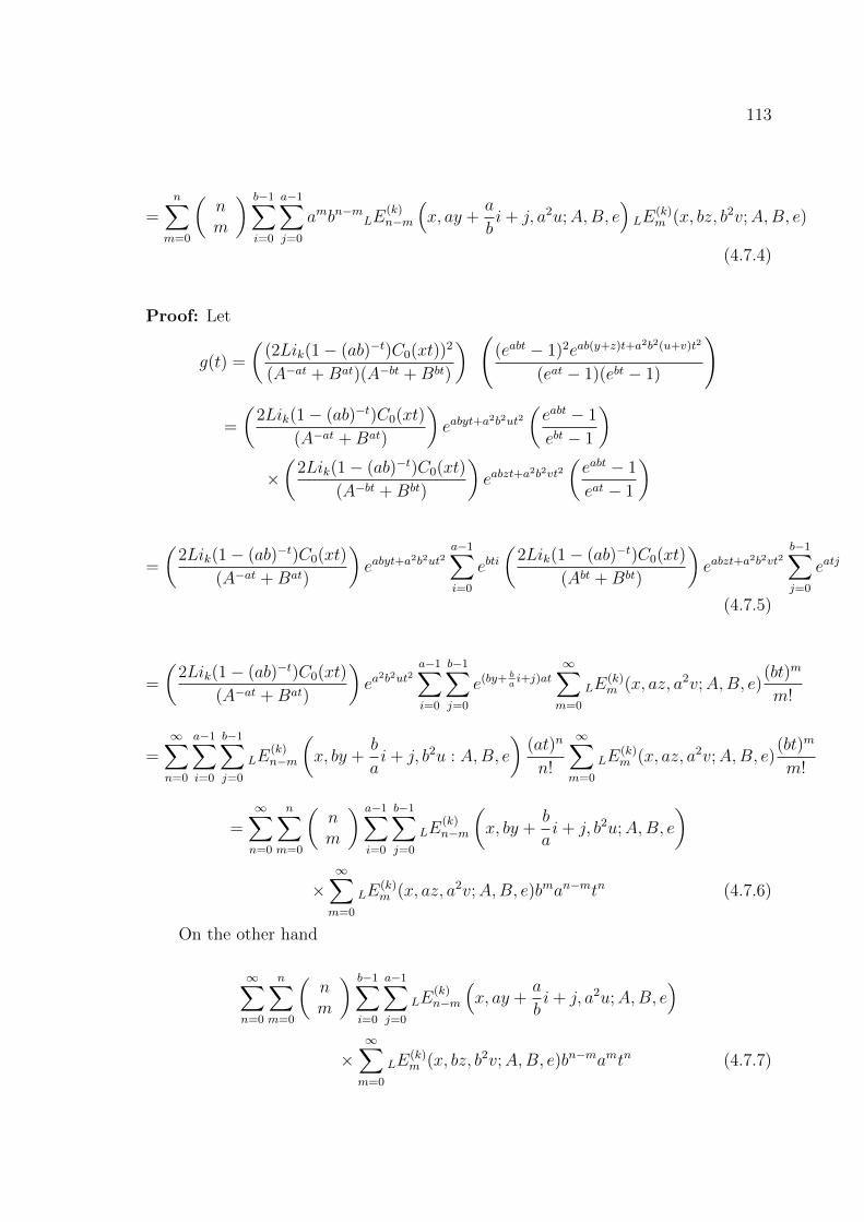
113

=n∑

m=0

(nm

) b−1∑i=0

a−1∑j=0

ambn−mLE(k)n−m

(x, ay +

a

bi+ j, a2u;A,B, e

)LE

(k)m (x, bz, b2v;A,B, e)

(4.7.4)

Proof: Let

g(t) =

((2Lik(1− (ab)−t)C0(xt))2

(A−at +Bat)(A−bt +Bbt)

) ((eabt − 1)2eab(y+z)t+a2b2(u+v)t2

(eat − 1)(ebt − 1)

)

=

(2Lik(1− (ab)−t)C0(xt)

(A−at +Bat)

)eabyt+a

2b2ut2(eabt − 1

ebt − 1

)×(

2Lik(1− (ab)−t)C0(xt)

(A−bt +Bbt)

)eabzt+a

2b2vt2(eabt − 1

eat − 1

)

=

(2Lik(1− (ab)−t)C0(xt)

(A−at +Bat)

)eabyt+a

2b2ut2a−1∑i=0

ebti(

2Lik(1− (ab)−t)C0(xt)

(Abt +Bbt)

)eabzt+a

2b2vt2b−1∑j=0

eatj

(4.7.5)

=

(2Lik(1− (ab)−t)C0(xt)

(A−at +Bat)

)ea

2b2ut2a−1∑i=0

b−1∑j=0

e(by+ bai+j)at

∞∑m=0

LE(k)m (x, az, a2v;A,B, e)

(bt)m

m!

=∞∑n=0

a−1∑i=0

b−1∑j=0

LE(k)n−m

(x, by +

b

ai+ j, b2u : A,B, e

)(at)n

n!

∞∑m=0

LE(k)m (x, az, a2v;A,B, e)

(bt)m

m!

=∞∑n=0

n∑m=0

(nm

) a−1∑i=0

b−1∑j=0

LE(k)n−m

(x, by +

b

ai+ j, b2u;A,B, e

)

×∞∑m=0

LE(k)m (x, az, a2v;A,B, e)bman−mtn (4.7.6)

On the other hand

∞∑n=0

n∑m=0

(nm

) b−1∑i=0

a−1∑j=0

LE(k)n−m

(x, ay +

a

bi+ j, a2u;A,B, e

)

×∞∑m=0

LE(k)m (x, bz, b2v;A,B, e)bn−mamtn (4.7.7)

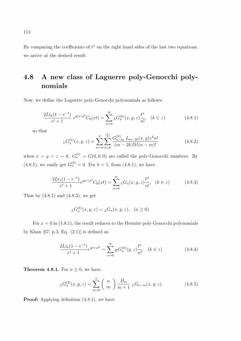
114

By comparing the coefficients of tn on the right hand sides of the last two equations,

we arrive at the desired result.

4.8 A new class of Laguerre poly-Genocchi poly-

nomials

Now, we define the Laguerre poly-Genocchi polynomials as follows:

2Lik(1− e−t)et + 1

eyt+zt2

C0(xt) =∞∑n=0

LG(k)n (x, y, z)

tn

n!, (k ∈ z) (4.8.1)

so that

LG(k)n (x, y, z) =

n∑m=0

[n2

]∑k=0

G(k)n−m Lm−2k(x, y)zkn!

(m− 2k)!k!(n−m)!(4.8.2)

when x = y = z = 0, G(k)n = G(0, 0, 0) are called the poly-Genocchi numbers. By

(4.8.1), we easily get G(k)n = 0. For k = 1, from (4.8.1), we have

2Li1(1− e−t)et + 1

eyt+zt2

C0(xt) =∞∑n=0

LGn(x, y, z)tn

n!, (k ∈ z) (4.8.3)

Thus by (4.8.1) and (4.8.3), we get

LG(k)n (x, y, z) = LGn(x, y, z), (n ≥ 0).

For x = 0 in (4.8.1), the result reduces to the Hermite poly-Genocchi polynomials

by Khan [67; p.3, Eq. (2.1)] is defined as

2Lik(1− e−t)et + 1

eyt+zt2

=∞∑n=0

HG(k)n (y, z)

tn

n!, (k ∈ z) (4.8.4)

Theorem 4.8.1. For n ≥ 0, we have

LG(2)n (x, y, z) =

n∑m=0

(nm

)Bm

m+ 1LGn−m(x, y, z) (4.8.5)

Proof: Applying definition (4.8.1), we have

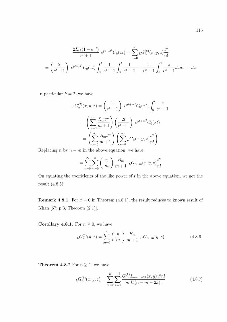
115

2Lik(1− e−t)et + 1

eyt+zt2

C0(xt) =∞∑n=0

LG(k)n (x, y, z)

tn

n!

=

(2

et + 1

)eyt+zt

2

C0(xt)

∫ t

0

1

ez − 1

∫ t

0

1

ez − 1· · · 1

ez − 1

∫ t

0

z

ez − 1dzdz · · · dz

In particular k = 2, we have

LG(2)n (x, y, z) =

(2

et + 1

)eyt+zt

2

C0(xt)

∫ t

0

z

ez − 1

=

(∞∑m=0

Bmtm

m+ 1

)(2t

et + 1

)eyt+zt

2

C0(xt)

=

(∞∑m=0

Bmtm

m+ 1

)(∞∑n=0

LGn(x, y, z)tn

n!

)Replacing n by n−m in the above equation, we have

=∞∑n=0

n∑m=0

(nm

)Bm

m+ 1LGn−m(x, y, z)

tn

n!

On equating the coefficients of the like power of t in the above equation, we get the

result (4.8.5).

Remark 4.8.1. For x = 0 in Theorem (4.8.1), the result reduces to known result of

Khan [67; p.3, Theorem (2.1)].

Corollary 4.8.1. For n ≥ 0, we have

LG(2)n (y, z) =

n∑m=0

(nm

)Bm

m+ 1HGn−m(y, z) (4.8.6)

Theorem 4.8.2 For n ≥ 1, we have

LG(k)n (x, y, z) =

n∑m=0

[n2

]∑k=0

G(k)m Ln−m−2k(x, y)zkn!

m!k!(n−m− 2k)!(4.8.7)

116

Proof: From equation (4.8.1), we have

∞∑n=0

LG(k)n (x, y, z)

tn

n!=

2Lik(1− e−t)et + 1

eyt+zt2

C0(xt)

=

(∞∑m=0

G(k)m

tm

m!

) ∞∑n=0

[n2

]∑k=0

Ln−2k(x, y)zk

k!(n− 2k)!tn

Replacing n by n −m in the above equation and comparing the coefficients of

tn, we get the result (4.8.7).

Remark 4.8.2. For x = 0 in Theorem (4.8.2), the result reduces to known result of

Khan [67; p.4, Theorem (2.2)].

Corollary 4.8.2. For n ≥ 1, we have

LG(k)n (y, z) =

n∑m=0

(nm

)G(k)m Ln−m(y, z) (4.8.8)

Theorem 4.8.3 For n ≥ 0, we have

LG(k)n (x, y, z) =

n∑p=0

p+1∑l=1

(−1)l+p+1l!S2(p+ 1, l)

lk(p+ 1)

(np

)LGn−p(x, y, z) (4.8.9)

Proof: From equation (4.8.1), we have

∞∑n=0

LG(k)n (x, y, z)

tn

n!=

(Lik(1− e−t)

t

) [(2t

et + 1

)eyt+zt

2

C0(xt)

](4.8.10)

Now1

tLik(1− e−t) =

1

t

∞∑l=1

(1− e−t)l

lk=

1

t

∞∑l=1

(−1)l

lk(1− e−t)l

=1

t

∞∑l=1

(−1)l

lkl!∞∑p=l

(−1)pS2(p, l)tp

p!

117

=1

t

∞∑p=1

p∑l=l

(−1)l+p

lkl!S2(p, l)

tp

p!

=∞∑p=0

(p+1∑l=l

(−1)l+p+1

lkl!S2(p+ 1, l)

p+ 1

)tp

p!(4.8.11)

From equation (4.8.10) and (4.8.11), we get

∞∑n=0

LG(k)n (x, y, z)

tn

n!=∞∑p=0

(p+1∑l=l

(−1)l+p+1

lkl!S2(p+ 1, l)

p+ 1

)tp

p!

(∞∑n=0

LGn(x, y, z)tn

n!

)

Replacing n by n− p in the r.h.s of above equation and comparing the coefficients of

tn, we get the result (4.8.9).

Remark 4.8.3. For x = 0 in Theorem (4.8.3), the result reduces to known result of

Khan [67; p.3, Theorem (2.3)].

Corollary 4.8.3. For n ≥ 0, we have

LG(k)n (y, z) =

n∑p=0

p+1∑l=1

(−1)l+p+1l!S2(p+ 1, l)

lk(p+ 1)

(np

)HGn−p(y, z) (4.8.12)

Theorem 4.8.4 For n ≥ 1, we have

LG(k)n (x, y + 1, z) + LG

(k)n (x, y, z) = 2

n∑p=1

p∑l=1

[n2

]∑k=0

(−1)l+p

lkl!n!S2(p, l)

Ln−p−2k(x, y)zk

p!k!(n− p− 2k)!

(4.8.13)

Proof: Using the definition (4.8.1), we have

∞∑n=0

LG(k)n (x, y + 1, z)

tn

n!+∞∑n=0

LG(k)n (x, y, z)

tn

n!

=2Lik(1− e−t)

et + 1e(y+1)t+zt2C0(xt) +

2Lik(1− e−t)et + 1

eyt+zt2

C0(xt)

118

= 2Lik(1− e−t) eyt+zt2

C0(xt)

=∞∑p=1

(2

p∑l=1

(−1)l+p

lkl!S2(p, l)

)tp

p!eyt+zt

2

C0(xt)

=∞∑p=1

(2

p∑l=1

(−1)l+p

lkl!S2(p, l)

)tp

p!

∞∑n=0

[n2

]∑k=0

Ln−2k(x, y)zk

k!(n− 2k)!tn

Replacing n by n− p in the above equation and comparing the coefficients of tn,

we get the result (4.8.13).

Remark 4.8.4. For x = 0 in Theorem (4.8.4), the result reduces to known result of

Khan [67; p.4, Theorem (2.4)].

Corollary 4.8.4. For n ≥ 1, we have

LG(k)n (y + 1, z) + LG

(k)n (y, z) = 2

n∑p=1

p∑l=1

(np

)(−1)l+pl!S2(p, l)Ln−p(y, z) (4.8.14)

Theorem 4.8.5 For d ∈ N with d ≡ 1(mod2), we have

LG(k)n (x, y, z) =

n∑p=0

(np

)dn−p−1

p+1∑l=0

d−1∑a=0

(−1)l+p+1l!S2(p+ 1, l)

lk(−1)aLGn−p

(x,a+ y

d, z

)(4.8.15)

Proof: From equation (4.8.1), we have

∞∑n=0

LG(k)n (x, y, z)

tn

n!=

2Lik(1− e−t)et + 1

eyt+zt2

C0(xt)

=

(2Lik(1− e−t)

t

)(2t

edt + 1

d−1∑a=0

e(a+y)t+zt2C0(xt)

)

=

(∞∑p=0

(p+1∑l=1

(−1)l+p+1

lkl!S2(p+ 1, l)

p+ 1

)tp

p!

)(∞∑m=0

dm−1

d−1∑a=0

(−1)aLGn

(x,a+ y

d, z

)tn

n!

)Replacing n by n− p in the above equation and comparing the coefficient of tn,

we get the result (4.8.15).

119

Remark 4.8.5. For x = 0 in Theorem (4.8.5), the result reduces to known result of

Khan [67; p.4, Theorem (2.5)].

Corollary 4.8.5. For d ∈ N with d ≡ 1(mod2), we have

LG(k)n (y, z) =

n∑p=0

(np

)dn−p−1

p+1∑l=0

d−1∑a=0

(−1)l+p+1l!S2(p+ 1, l)

lk(−1)aLGn−p

(a+ y

d, z

)(4.8.16)

4.9 Implicit summation formulae involving Laguerre

poly-Genocchi polynomials

For the derivation of implicit formulae involving poly-Genocchi polynomials G(k)n

and Laguerre poly-Genocchi polynomials LG(k)n (x, y, z) the same considerations are

developed for the ordinary Hermite and related polynomials in Khan et al. [84]

and Hermite-Bernoulli polynomials in Pathan and Khan [117-118] holds as well.

First we prove the following results involving Laguerre poly-Genocchi polynomials

LG(k)n (x, y, z).

Theorem 4.9.1. For x, y, z ∈ R and n ≥ 0, the following implicit summation for-

mula for Laguerre poly-Genocchi polynomials LG(k)n (x, y, z) holds true:

LG(k)l+p(x, v, z) =

l,p∑m,n=0

(lm

)(pn

)(v − y)m+n

LG(k)l+p−m−n(x, y, z) (4.9.1)

Proof: We replace t by t+ u and rewrite the generating function (4.8.1) as(2Lik(1− e−(t+u))

et+u + 1

)ez(t+u)2C0(x(t+u)) = e−y(t+u)

∞∑l,p=0

LG(k)l+p(x, y, z)

tl

l!

up

p!(4.9.2)

Replacing y by v in the above equation and equating the resulting equation to the

above equation, we get

e(v−y)(t+u)

∞∑l,p=0

LG(k)l+p(x, y, z)

tl

l!

up

p!=

∞∑l,p=0

LG(k)l+p(x, v, z)

tl

l!

up

p!(4.9.3)

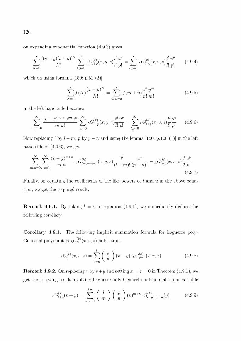
120

on expanding exponential function (4.9.3) gives

∞∑N=0

[(v − y)(t+ u)]N

N !

∞∑l,p=0

LG(k)l+p(x, y, z)

tl

l!

up

p!=

∞∑l,p=0

LG(k)l+p(x, v, z)

tl

l!

up

p!(4.9.4)

which on using formula [150; p.52 (2)]

∞∑N=0

f(N)(x+ y)N

N !=

∞∑m,n=0

f(m+ n)xn

n!

ym

m!(4.9.5)

in the left hand side becomes

∞∑m,n=0

(v − y)m+n tmun

m!n!

∞∑l,p=0

LG(k)l+p(x, y, z)

tl

l!

up

p!=

∞∑l,p=0

LG(k)l+p(x, v, z)

tl

l!

up

p!(4.9.6)

Now replacing l by l−m, p by p− n and using the lemma [150; p.100 (1)] in the left

hand side of (4.9.6), we get

∞∑m,n=0

∞∑l,p=0

(v − y)m+n

m!n!LG

(k)l+p−m−n(x, y, z)

tl

(l −m)!

up

(p− n)!= LG

(k)l+p(x, v, z)

tl

l!

up

p!

(4.9.7)

Finally, on equating the coefficients of the like powers of t and u in the above equa-

tion, we get the required result.

Remark 4.9.1. By taking l = 0 in equation (4.9.1), we immediately deduce the

following corollary.

Corollary 4.9.1. The following implicit summation formula for Laguerre poly-

Genocchi polynomials LG(k)n (x, v, z) holds true:

LG(k)p (x, v, z) =

p∑n=0

(pn

)(v − y)nLG

(k)p−n(x, y, z) (4.9.8)

Remark 4.9.2. On replacing v by v+y and setting x = z = 0 in Theorem (4.9.1), we

get the following result involving Laguerre poly-Genocchi polynomial of one variable

LG(k)l+p(v + y) =

l,p∑m,n=0

(lm

)(pn

)(v)m+n

LG(k)l+p−m−n(y) (4.9.9)

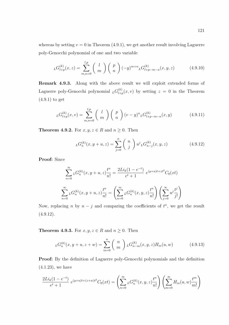
121

whereas by setting v = 0 in Theorem (4.9.1), we get another result involving Laguerre

poly-Genocchi polynomial of one and two variable

LG(k)l+p(x, z) =

l,p∑m,n=0

(lm

)(pn

)(−y)m+n

LG(k)l+p−m−n(x, y, z) (4.9.10)

Remark 4.9.3. Along with the above result we will exploit extended forms of

Laguerre poly-Genocchi polynomial LG(k)l+p(x, v) by setting z = 0 in the Theorem

(4.9.1) to get

LG(k)l+p(x, v) =

l,p∑m,n=0

(lm

)(pn

)(v − y)nLG

(k)l+p−m−n(x, y) (4.9.11)

Theorem 4.9.2. For x, y, z ∈ R and n ≥ 0. Then

LG(k)n (x, y + u, z) =

n∑j=0

(nj

)ujLG

(k)n−j(x, y, z) (4.9.12)

Proof: Since

∞∑n=0

LG(k)n (x, y + u, z)

tn

n!=

2Lik(1− e−t)et + 1

e(y+u)t+zt2C0(xt)

∞∑n=0

LG(k)n (x, y + u, z)

tn

n!=

(∞∑n=0

LG(k)n (x, y, z)

tn

n!

)(∞∑j=0

ujtj

j!

)Now, replacing n by n − j and comparing the coefficients of tn, we get the result

(4.9.12).

Theorem 4.9.3. For x, y, z ∈ R and n ≥ 0. Then

LG(k)n (x, y + u, z + w) =

n∑m=0

(nm

)LG

(k)n−m(x, y, z)Hm(u,w) (4.9.13)

Proof: By the definition of Laguerre poly-Genocchi polynomials and the definition

(4.1.23), we have

2Lik(1− e−t)et + 1

e(y+u)t+(z+w)t2C0(xt) =

(∞∑n=0

LG(k)n (x, y, z)

tn

n!

)(∞∑m=0

Hm(u,w)tm

m!

)

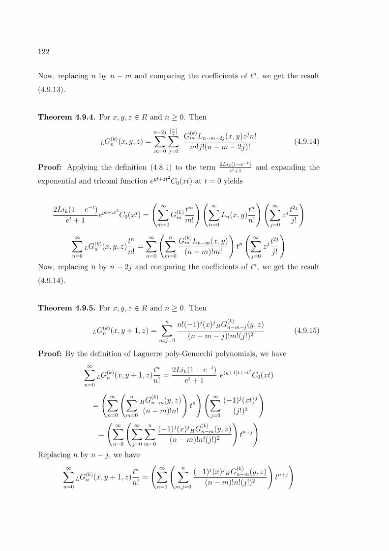
122

Now, replacing n by n − m and comparing the coefficients of tn, we get the result

(4.9.13).

Theorem 4.9.4. For x, y, z ∈ R and n ≥ 0. Then

LG(k)n (x, y, z) =

n−2j∑m=0

[n2

]∑j=0

G(k)m Ln−m−2j(x, y)zjn!

m!j!(n−m− 2j)!(4.9.14)

Proof: Applying the definition (4.8.1) to the term 2Lik(1−e−t)et+1

and expanding the

exponential and tricomi function eyt+zt2C0(xt) at t = 0 yields

2Lik(1− e−t)et + 1

eyt+zt2

C0(xt) =

(∞∑m=0

G(k)m

tm

m!

)(∞∑n=0

Ln(x, y)tn

n!

)(∞∑j=0

zjt2j

j!

)∞∑n=0

LG(k)n (x, y, z)

tn

n!=∞∑n=0

(n∑

m=0

G(k)m Ln−m(x, y)

(n−m)!m!

)tn

(∞∑j=0

zjt2j

j!

)Now, replacing n by n − 2j and comparing the coefficients of tn, we get the result

(4.9.14).

Theorem 4.9.5. For x, y, z ∈ R and n ≥ 0. Then

LG(k)n (x, y + 1, z) =

n∑m,j=0

n!(−1)j(x)jHG(k)n−m−j(y, z)

(n−m− j)!m!(j!)2(4.9.15)

Proof: By the definition of Laguerre poly-Genocchi polynomials, we have

∞∑n=0

LG(k)n (x, y + 1, z)

tn

n!=

2Lik(1− e−t)et + 1

e(y+1)t+zt2C0(xt)

=

(∞∑n=0

(n∑

m=0

HG(k)n−m(y, z)

(n−m)!n!

)tn

)(∞∑j=0

(−1)j(xt)j

(j!)2

)

=

(∞∑n=0

(∞∑j=0

n∑m=0

(−1)j(x)jHG(k)n−m(y, z)

(n−m)!n!(j!)2

)tn+j

)Replacing n by n− j, we have

∞∑n=0

LG(k)n (x, y + 1, z)

tn

n!=

(∞∑n=0

(n∑

m,j=0

(−1)j(x)jHG(k)n−m(y, z)

(n−m)!n!(j!)2

)tn+j

)

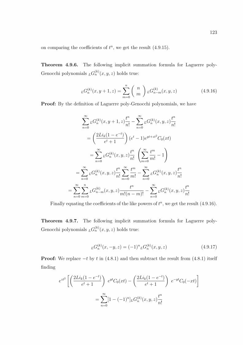
123

on comparing the coefficients of tn, we get the result (4.9.15).

Theorem 4.9.6. The following implicit summation formula for Laguerre poly-

Genocchi polynomials LG(k)n (x, y, z) holds true:

LG(k)n (x, y + 1, z) =

n∑m=0

(nm

)LG

(k)n−m(x, y, z) (4.9.16)

Proof: By the definition of Laguerre poly-Genocchi polynomials, we have

∞∑n=0

LG(k)n (x, y + 1, z)

tn

n!−∞∑n=0

LG(k)n (x, y, z)

tn

n!

=

(2Lik(1− e−t)

et + 1

)(et − 1)eyt+zt

2

C0(xt)

=∞∑n=0

LG(k)n (x, y, z)

tn

n!

(∞∑m=0

tm

m!− 1

)

=∞∑n=0

LG(k)n (x, y, z)

tn

n!

∞∑m=0

tm

m!−∞∑n=0

LG(k)n (x, y, z)

tn

n!

=∞∑n=0

n∑m=0

LG(k)n−m(x, y, z)

tn

m!(n−m)!−∞∑n=0

LG(k)n (x, y, z)

tn

n!

Finally equating the coefficients of the like powers of tn, we get the result (4.9.16).

Theorem 4.9.7. The following implicit summation formula for Laguerre poly-

Genocchi polynomials LG(k)n (x, y, z) holds true:

LG(k)n (x,−y, z) = (−1)nLG

(k)n (x, y, z) (4.9.17)

Proof: We replace −t by t in (4.8.1) and then subtract the result from (4.8.1) itself

finding

ezt2

[(2Lik(1− e−t)

et + 1

)eytC0(xt)−

(2Lik(1− e−t)

et + 1

)e−ytC0(−xt)

]

=∞∑n=0

[1− (−1)n]LG(k)n (x, y, z)

tn

n!

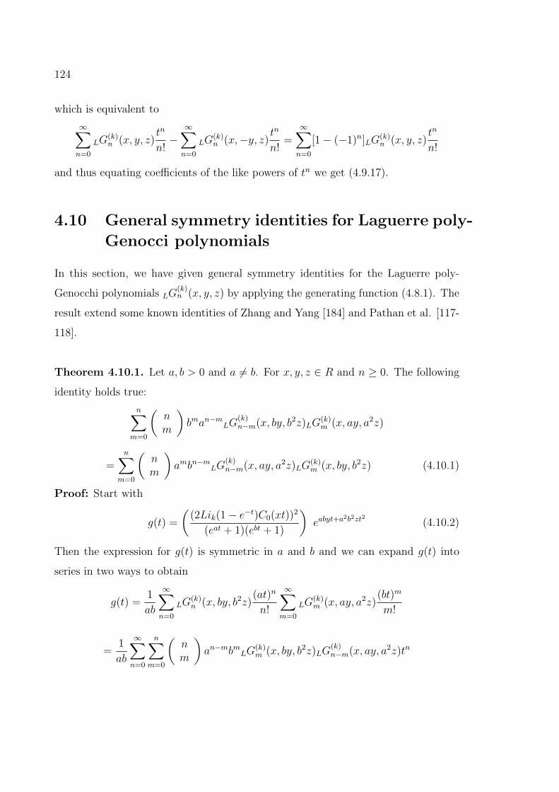
124

which is equivalent to

∞∑n=0

LG(k)n (x, y, z)

tn

n!−∞∑n=0

LG(k)n (x,−y, z) t

n

n!=∞∑n=0

[1− (−1)n]LG(k)n (x, y, z)

tn

n!

and thus equating coefficients of the like powers of tn we get (4.9.17).

4.10 General symmetry identities for Laguerre poly-

Genocci polynomials

In this section, we have given general symmetry identities for the Laguerre poly-

Genocchi polynomials LG(k)n (x, y, z) by applying the generating function (4.8.1). The

result extend some known identities of Zhang and Yang [184] and Pathan et al. [117-

118].

Theorem 4.10.1. Let a, b > 0 and a 6= b. For x, y, z ∈ R and n ≥ 0. The following

identity holds true:

n∑m=0

(nm

)bman−mLG

(k)n−m(x, by, b2z)LG

(k)m (x, ay, a2z)

=n∑

m=0

(nm

)ambn−mLG

(k)n−m(x, ay, a2z)LG

(k)m (x, by, b2z) (4.10.1)

Proof: Start with

g(t) =

((2Lik(1− e−t)C0(xt))2

(eat + 1)(ebt + 1)

)eabyt+a

2b2zt2 (4.10.2)

Then the expression for g(t) is symmetric in a and b and we can expand g(t) into

series in two ways to obtain

g(t) =1

ab

∞∑n=0

LG(k)n (x, by, b2z)

(at)n

n!

∞∑m=0

LG(k)m (x, ay, a2z)

(bt)m

m!

=1

ab

∞∑n=0

n∑m=0

(nm

)an−mbmLG

(k)m (x, by, b2z)LG

(k)n−m(x, ay, a2z)tn

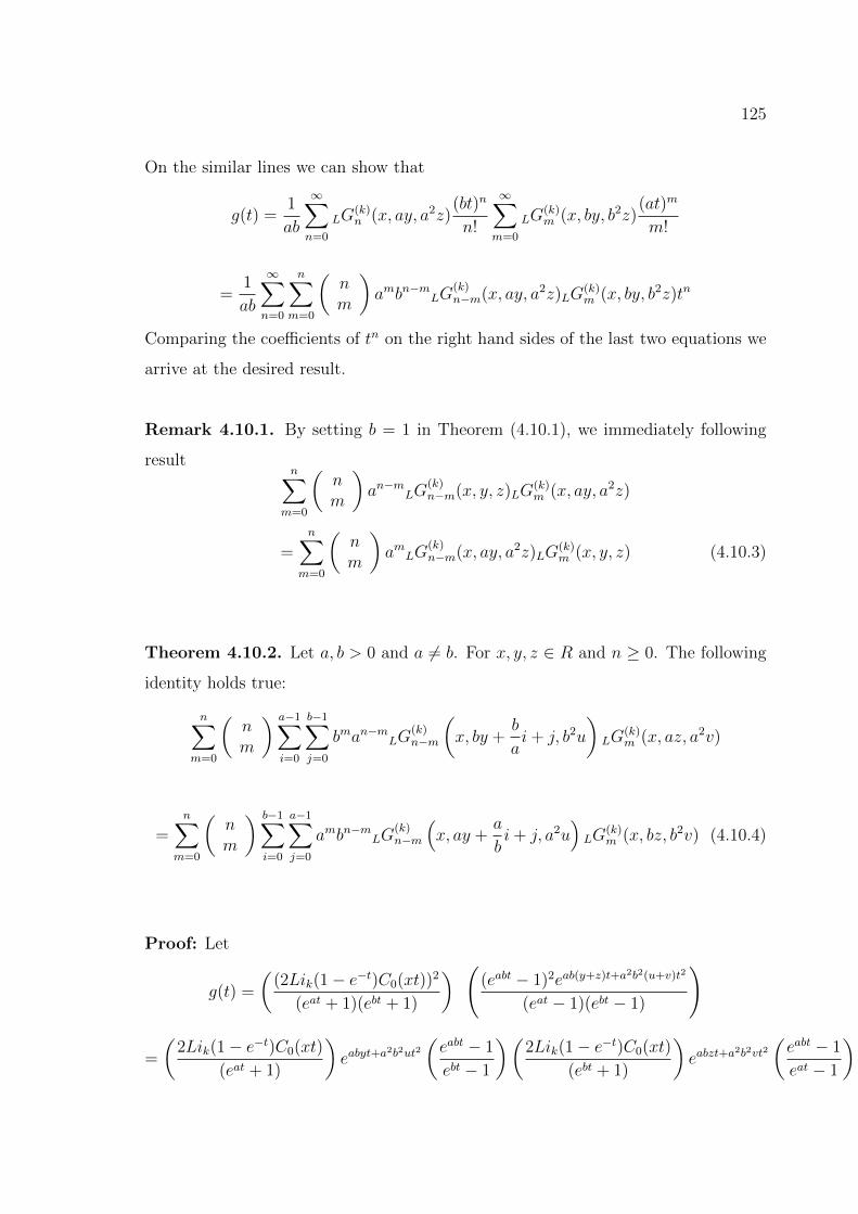
125

On the similar lines we can show that

g(t) =1

ab

∞∑n=0

LG(k)n (x, ay, a2z)

(bt)n

n!

∞∑m=0

LG(k)m (x, by, b2z)

(at)m

m!

=1

ab

∞∑n=0

n∑m=0

(nm

)ambn−mLG

(k)n−m(x, ay, a2z)LG

(k)m (x, by, b2z)tn

Comparing the coefficients of tn on the right hand sides of the last two equations we

arrive at the desired result.

Remark 4.10.1. By setting b = 1 in Theorem (4.10.1), we immediately following

resultn∑

m=0

(nm

)an−mLG

(k)n−m(x, y, z)LG

(k)m (x, ay, a2z)

=n∑

m=0

(nm

)amLG

(k)n−m(x, ay, a2z)LG

(k)m (x, y, z) (4.10.3)

Theorem 4.10.2. Let a, b > 0 and a 6= b. For x, y, z ∈ R and n ≥ 0. The following

identity holds true:

n∑m=0

(nm

) a−1∑i=0

b−1∑j=0

bman−mLG(k)n−m

(x, by +

b

ai+ j, b2u

)LG

(k)m (x, az, a2v)

=n∑

m=0

(nm

) b−1∑i=0

a−1∑j=0

ambn−mLG(k)n−m

(x, ay +

a

bi+ j, a2u

)LG

(k)m (x, bz, b2v) (4.10.4)

Proof: Let

g(t) =

((2Lik(1− e−t)C0(xt))2

(eat + 1)(ebt + 1)

) ((eabt − 1)2eab(y+z)t+a2b2(u+v)t2

(eat − 1)(ebt − 1)

)

=

(2Lik(1− e−t)C0(xt)

(eat + 1)

)eabyt+a

2b2ut2(eabt − 1

ebt − 1

)(2Lik(1− e−t)C0(xt)

(ebt + 1)

)eabzt+a

2b2vt2(eabt − 1

eat − 1

)

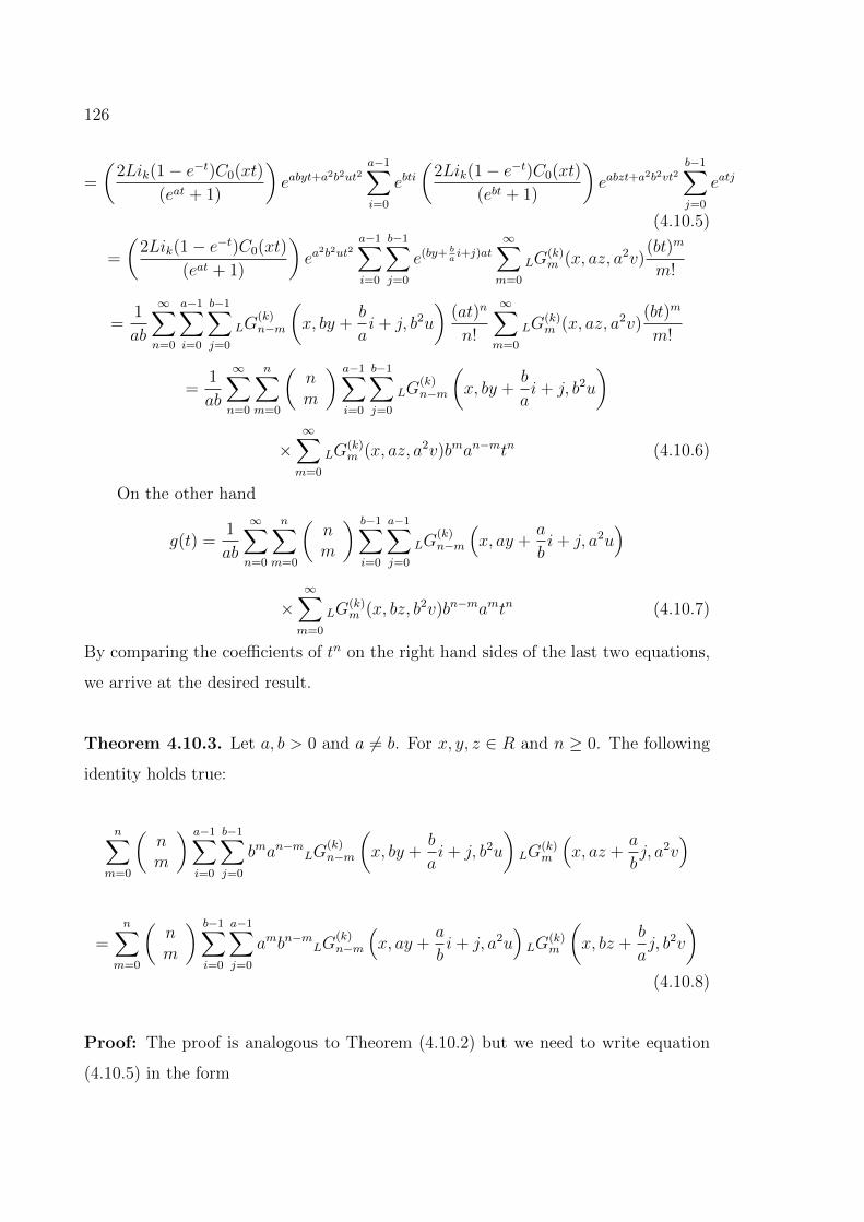
126

=

(2Lik(1− e−t)C0(xt)

(eat + 1)

)eabyt+a

2b2ut2a−1∑i=0

ebti(

2Lik(1− e−t)C0(xt)

(ebt + 1)

)eabzt+a

2b2vt2b−1∑j=0

eatj

(4.10.5)

=

(2Lik(1− e−t)C0(xt)

(eat + 1)

)ea

2b2ut2a−1∑i=0

b−1∑j=0

e(by+ bai+j)at

∞∑m=0

LG(k)m (x, az, a2v)

(bt)m

m!

=1

ab

∞∑n=0

a−1∑i=0

b−1∑j=0

LG(k)n−m

(x, by +

b

ai+ j, b2u

)(at)n

n!

∞∑m=0

LG(k)m (x, az, a2v)

(bt)m

m!

=1

ab

∞∑n=0

n∑m=0

(nm

) a−1∑i=0

b−1∑j=0

LG(k)n−m

(x, by +

b

ai+ j, b2u

)

×∞∑m=0

LG(k)m (x, az, a2v)bman−mtn (4.10.6)

On the other hand

g(t) =1

ab

∞∑n=0

n∑m=0

(nm

) b−1∑i=0

a−1∑j=0

LG(k)n−m

(x, ay +

a

bi+ j, a2u

)

×∞∑m=0

LG(k)m (x, bz, b2v)bn−mamtn (4.10.7)

By comparing the coefficients of tn on the right hand sides of the last two equations,

we arrive at the desired result.

Theorem 4.10.3. Let a, b > 0 and a 6= b. For x, y, z ∈ R and n ≥ 0. The following

identity holds true:

n∑m=0

(nm

) a−1∑i=0

b−1∑j=0

bman−mLG(k)n−m

(x, by +

b

ai+ j, b2u

)LG

(k)m

(x, az +

a

bj, a2v

)

=n∑

m=0

(nm

) b−1∑i=0

a−1∑j=0

ambn−mLG(k)n−m

(x, ay +

a

bi+ j, a2u

)LG

(k)m

(x, bz +

b

aj, b2v

)(4.10.8)

Proof: The proof is analogous to Theorem (4.10.2) but we need to write equation

(4.10.5) in the form

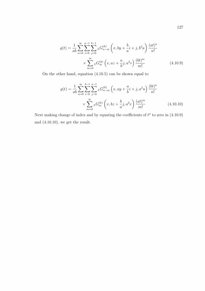
127

g(t) =1

ab

∞∑n=0

a−1∑i=0

b−1∑j=0

LG(k)n−m

(x, by +

b

ai+ j, b2u

)(at)n

n!

×∞∑m=0

LG(k)m

(x, az +

a

bj, a2v

) (bt)m

m!(4.10.9)

On the other hand, equation (4.10.5) can be shown equal to

g(t) =1

ab

∞∑n=0

b−1∑i=0

a−1∑j=0

LG(k)n−m

(x, ay +

a

bi+ j, a2u

) (bt)n

n!

×∞∑m=0

LG(k)m

(x, bz +

b

aj, a2v

)(at)m

m!(4.10.10)

Next making change of index and by equating the coefficients of tn to zero in (4.10.9)

and (4.10.10), we get the result.

Chapter 5

New Presentations of theGeneralized Voigt Function withDifferent Parameters

5.1 Introduction

This chapter deals with the new generalization of the Voigt functions K(x, y) and

L(x, y) which were introduced by Voigt in 1899. These functions occur in great

diversity in astrophysical spectroscopy, neutron physics, plasma physics and statis-

tical communication theory, as well as in some areas of mathematical physics and

engineering associated with multi-dimensional analysis of spectral harmonics.

Furthermore, the function K(x, y) + iL(x, y) is, except for a numerical factor,

identical to the so-called plasma dispersion function, which is tabulated by Fried and

Conte [49].

In any given physical problem, a numerical or analytical evaluation of the Voigt

function K(x, y) and L(x, y) (or of their aforementioned variants) is required. For a

review of various mathematical properties and computational methods concerning the

Voigt functions, see (for example) Srivastava and Chen [156], Srivastava et al. [170],

Pathan and Shahwan [124], Goyal and Mukherjee [52], Gupta et al. [55], Pathan et

al. [127], Pathan et al. [128], Garg and Jain [50], Gupta and Gupta [54], Khan and

Ghayasuddin [76] and Khan et al. [81].

For the purposes of our present study, we begin by recalling here the following

128

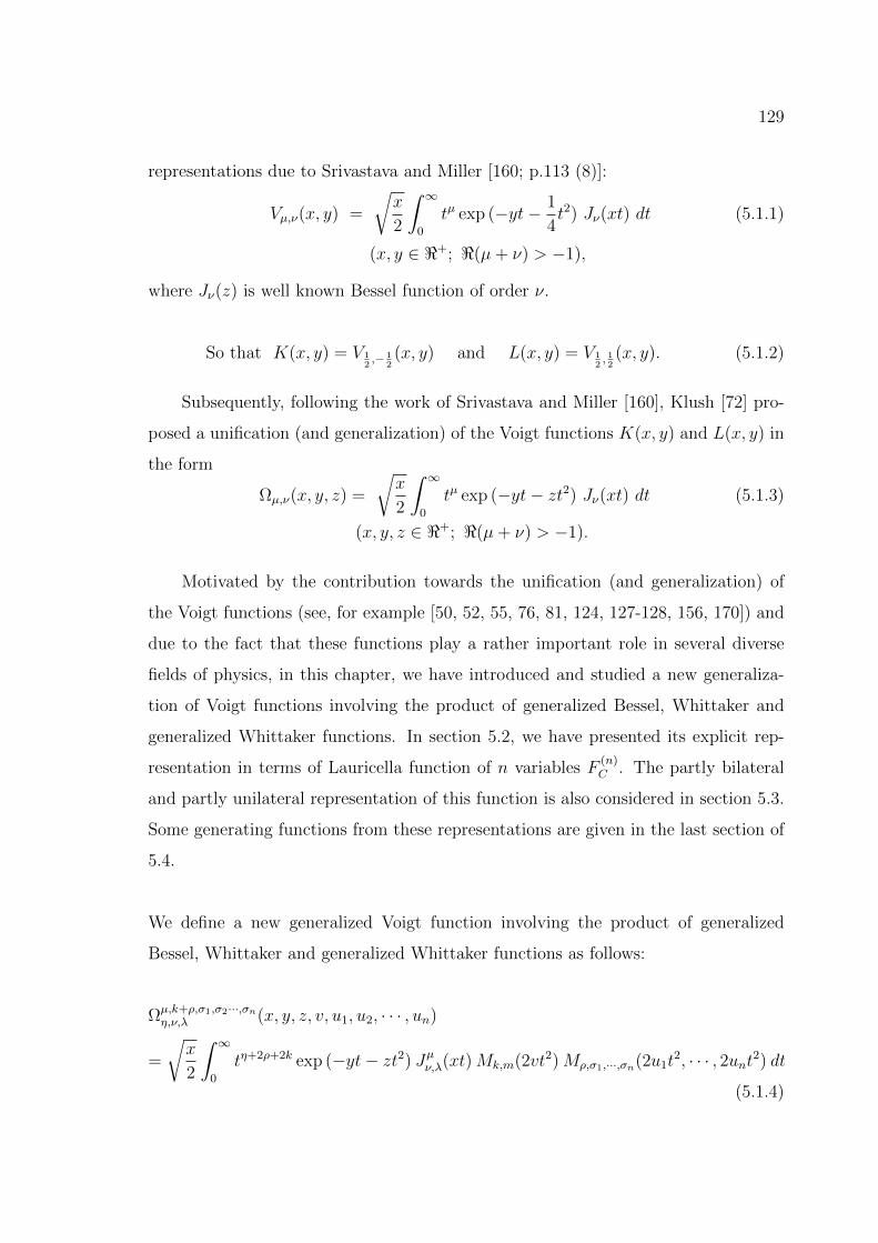
129

representations due to Srivastava and Miller [160; p.113 (8)]:

Vµ,ν(x, y) =

√x

2

∫ ∞0

tµ exp (−yt− 1

4t2) Jν(xt) dt (5.1.1)

(x, y ∈ <+; <(µ+ ν) > −1),

where Jν(z) is well known Bessel function of order ν.

So that K(x, y) = V 12,− 1

2(x, y) and L(x, y) = V 1

2, 12(x, y). (5.1.2)

Subsequently, following the work of Srivastava and Miller [160], Klush [72] pro-

posed a unification (and generalization) of the Voigt functions K(x, y) and L(x, y) in

the form

Ωµ,ν(x, y, z) =

√x

2

∫ ∞0

tµ exp (−yt− zt2) Jν(xt) dt (5.1.3)

(x, y, z ∈ <+; <(µ+ ν) > −1).

Motivated by the contribution towards the unification (and generalization) of

the Voigt functions (see, for example [50, 52, 55, 76, 81, 124, 127-128, 156, 170]) and

due to the fact that these functions play a rather important role in several diverse

fields of physics, in this chapter, we have introduced and studied a new generaliza-

tion of Voigt functions involving the product of generalized Bessel, Whittaker and

generalized Whittaker functions. In section 5.2, we have presented its explicit rep-

resentation in terms of Lauricella function of n variables F(n)C . The partly bilateral

and partly unilateral representation of this function is also considered in section 5.3.

Some generating functions from these representations are given in the last section of

5.4.

We define a new generalized Voigt function involving the product of generalized

Bessel, Whittaker and generalized Whittaker functions as follows:

Ωµ,k+ρ,σ1,σ2···,σnη,ν,λ (x, y, z, v, u1, u2, · · · , un)

=

√x

2

∫ ∞0

tη+2ρ+2k exp (−yt− zt2) Jµν,λ(xt)Mk,m(2vt2)Mρ,σ1,···,σn(2u1t2, · · · , 2unt2) dt

(5.1.4)

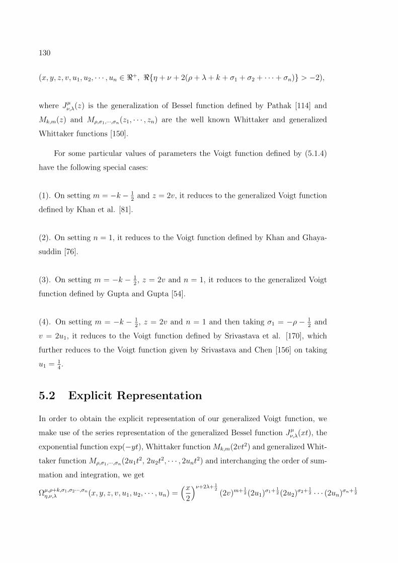
130

(x, y, z, v, u1, u2, · · · , un ∈ <+, <η + ν + 2(ρ+ λ+ k + σ1 + σ2 + · · ·+ σn) > −2),

where Jµν,λ(z) is the generalization of Bessel function defined by Pathak [114] and

Mk,m(z) and Mρ,σ1,···,σn(z1, · · · , zn) are the well known Whittaker and generalized

Whittaker functions [150].

For some particular values of parameters the Voigt function defined by (5.1.4)

have the following special cases:

(1). On setting m = −k− 12

and z = 2v, it reduces to the generalized Voigt function

defined by Khan et al. [81].

(2). On setting n = 1, it reduces to the Voigt function defined by Khan and Ghaya-

suddin [76].

(3). On setting m = −k − 12, z = 2v and n = 1, it reduces to the generalized Voigt

function defined by Gupta and Gupta [54].

(4). On setting m = −k − 12, z = 2v and n = 1 and then taking σ1 = −ρ − 1

2and

v = 2u1, it reduces to the Voigt function defined by Srivastava et al. [170], which

further reduces to the Voigt function given by Srivastava and Chen [156] on taking

u1 = 14.

5.2 Explicit Representation

In order to obtain the explicit representation of our generalized Voigt function, we

make use of the series representation of the generalized Bessel function Jµν,λ(xt), the

exponential function exp(−yt), Whittaker function Mk,m(2vt2) and generalized Whit-

taker function Mρ,σ1,···,σn(2u1t2, 2u2t

2, · · · , 2unt2) and interchanging the order of sum-

mation and integration, we get

Ωµ,ρ+k,σ1,σ2···,σnη,ν,λ (x, y, z, v, u1, u2, · · · , un) =

(x2

)ν+2λ+ 12

(2v)m+ 12 (2u1)σ1+ 1

2 (2u2)σ2+ 12 · · · (2un)σn+ 1

2

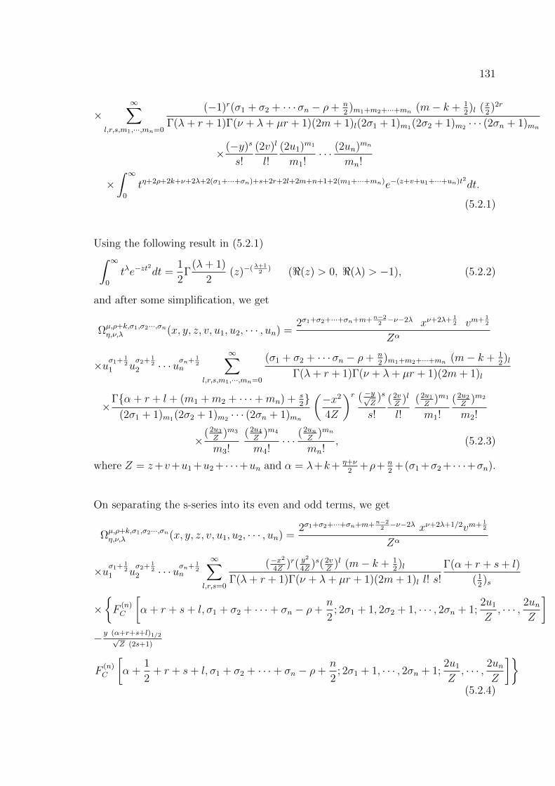
131

×∞∑

l,r,s,m1,···,mn=0

(−1)r(σ1 + σ2 + · · ·σn − ρ+ n2)m1+m2+···+mn (m− k + 1

2)l (x

2)2r

Γ(λ+ r + 1)Γ(ν + λ+ µr + 1)(2m+ 1)l(2σ1 + 1)m1(2σ2 + 1)m2 · · · (2σn + 1)mn

×(−y)s

s!

(2v)l

l!

(2u1)m1

m1!· · · (2un)mn

mn!

×∫ ∞

0

tη+2ρ+2k+ν+2λ+2(σ1+···+σn)+s+2r+2l+2m+n+1+2(m1+···+mn)e−(z+v+u1+···+un)t2dt.

(5.2.1)

Using the following result in (5.2.1)∫ ∞0

tλe−zt2

dt =1

2Γ

(λ+ 1)

2(z)−(λ+1

2) (<(z) > 0, <(λ) > −1), (5.2.2)

and after some simplification, we get

Ωµ,ρ+k,σ1,σ2···,σnη,ν,λ (x, y, z, v, u1, u2, · · · , un) =

2σ1+σ2+···+σn+m+n−22−ν−2λ xν+2λ+ 1

2 vm+ 12

Zα

×uσ1+ 12

1 uσ2+ 1

22 · · ·uσn+ 1

2n

∞∑l,r,s,m1,···,mn=0

(σ1 + σ2 + · · · σn − ρ+ n2)m1+m2+···+mn (m− k + 1

2)l

Γ(λ+ r + 1)Γ(ν + λ+ µr + 1)(2m+ 1)l

×Γα + r + l + (m1 +m2 + · · ·+mn) + s

2

(2σ1 + 1)m1(2σ2 + 1)m2 · · · (2σn + 1)mn

(−x2

4Z

)r ( −y√Z

)s

s!

(2vZ

)l

l!

(2u1Z

)m1

m1!

(2u2Z

)m2

m2!

×(2u3Z

)m3

m3!

(2u4Z

)m4

m4!· · ·

(2unZ

)mn

mn!, (5.2.3)

where Z = z+v+u1 +u2 + · · ·+un and α = λ+k+ η+ν2

+ρ+ n2

+(σ1 +σ2 + · · ·+σn).

On separating the s-series into its even and odd terms, we get

Ωµ,ρ+k,σ1,σ2···,σnη,ν,λ (x, y, z, v, u1, u2, · · · , un) =

2σ1+σ2+···+σn+m+n−22−ν−2λ xν+2λ+1/2vm+ 1

2

Zα

×uσ1+ 12

1 uσ2+ 1

22 · · ·uσn+ 1

2n

∞∑l,r,s=0

(−x2

4Z)r( y

2

4Z)s(2v

Z)l (m− k + 1

2)l

Γ(λ+ r + 1)Γ(ν + λ+ µr + 1)(2m+ 1)l l! s!

Γ(α + r + s+ l)

(12)s

×F

(n)C

[α + r + s+ l, σ1 + σ2 + · · ·+ σn − ρ+

n

2; 2σ1 + 1, 2σ2 + 1, · · · , 2σn + 1;

2u1

Z, · · · , 2un

Z

]−y (α+r+s+l)1/2√

Z (2s+1)

F(n)C

[α +

1

2+ r + s+ l, σ1 + σ2 + · · ·+ σn − ρ+

n

2; 2σ1 + 1, · · · , 2σn + 1;

2u1

Z, · · · , 2un

Z

](5.2.4)

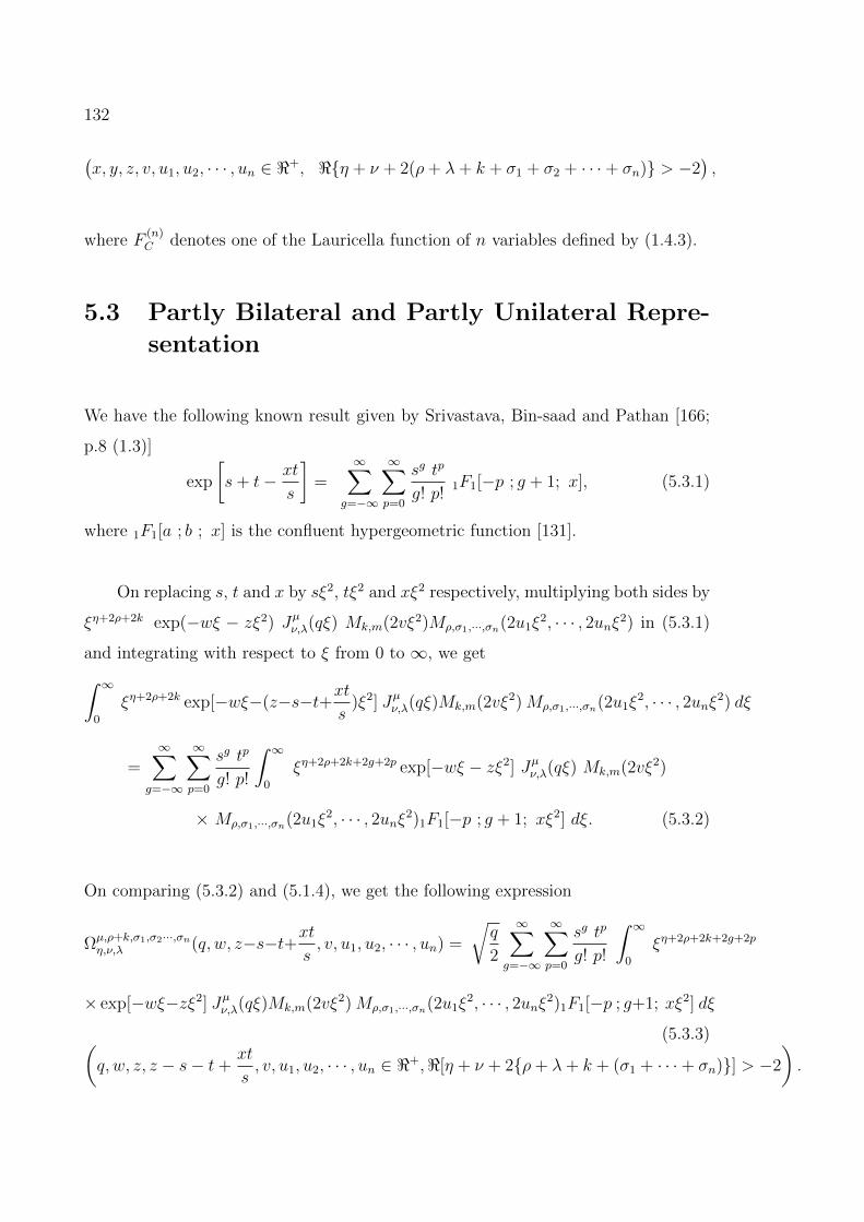
132

(x, y, z, v, u1, u2, · · · , un ∈ <+, <η + ν + 2(ρ+ λ+ k + σ1 + σ2 + · · ·+ σn) > −2

),

where F(n)C denotes one of the Lauricella function of n variables defined by (1.4.3).

5.3 Partly Bilateral and Partly Unilateral Repre-

sentation

We have the following known result given by Srivastava, Bin-saad and Pathan [166;

p.8 (1.3)]

exp

[s+ t− xt

s

]=

∞∑g=−∞

∞∑p=0

sg tp

g! p!1F1[−p ; g + 1; x], (5.3.1)

where 1F1[a ; b ; x] is the confluent hypergeometric function [131].

On replacing s, t and x by sξ2, tξ2 and xξ2 respectively, multiplying both sides by

ξη+2ρ+2k exp(−wξ − zξ2) Jµν,λ(qξ) Mk,m(2vξ2)Mρ,σ1,···,σn(2u1ξ2, · · · , 2unξ2) in (5.3.1)

and integrating with respect to ξ from 0 to ∞, we get∫ ∞0

ξη+2ρ+2k exp[−wξ−(z−s−t+xts

)ξ2] Jµν,λ(qξ)Mk,m(2vξ2)Mρ,σ1,···,σn(2u1ξ2, · · · , 2unξ2) dξ

=∞∑

g=−∞

∞∑p=0

sg tp

g! p!

∫ ∞0

ξη+2ρ+2k+2g+2p exp[−wξ − zξ2] Jµν,λ(qξ) Mk,m(2vξ2)

× Mρ,σ1,···,σn(2u1ξ2, · · · , 2unξ2)1F1[−p ; g + 1; xξ2] dξ. (5.3.2)

On comparing (5.3.2) and (5.1.4), we get the following expression

Ωµ,ρ+k,σ1,σ2···,σnη,ν,λ (q, w, z−s−t+xt

s, v, u1, u2, · · · , un) =

√q

2

∞∑g=−∞

∞∑p=0

sg tp

g! p!

∫ ∞0

ξη+2ρ+2k+2g+2p

× exp[−wξ−zξ2] Jµν,λ(qξ)Mk,m(2vξ2)Mρ,σ1,···,σn(2u1ξ2, · · · , 2unξ2)1F1[−p ; g+1; xξ2] dξ

(5.3.3)(q, w, z, z − s− t+

xt

s, v, u1, u2, · · · , un ∈ <+,<[η + ν + 2ρ+ λ+ k + (σ1 + · · ·+ σn)] > −2

).

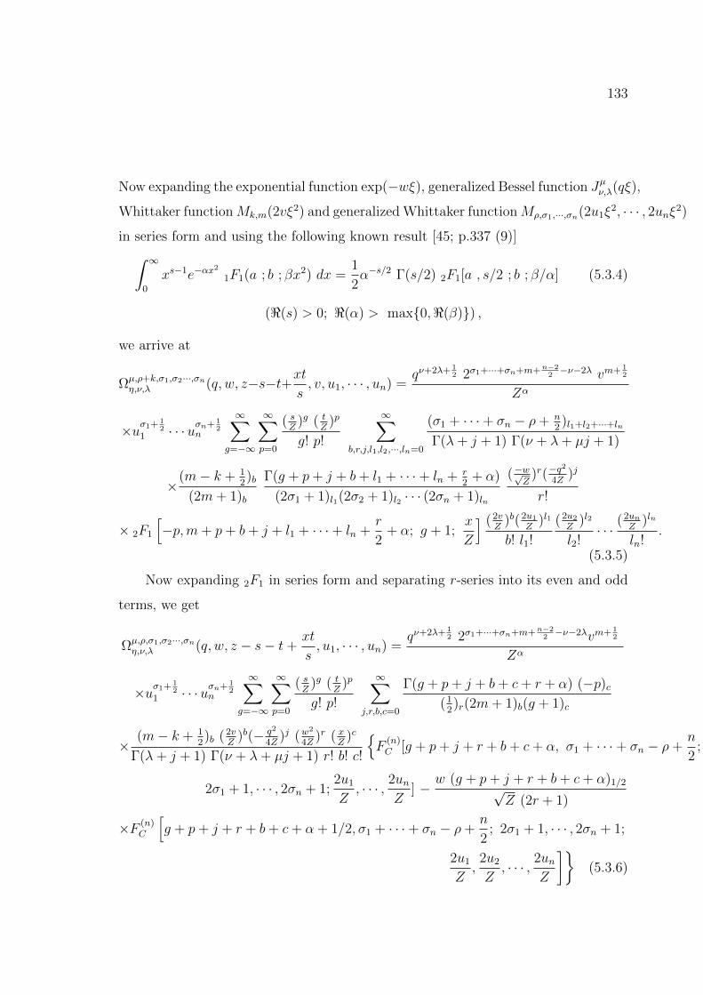
133

Now expanding the exponential function exp(−wξ), generalized Bessel function Jµν,λ(qξ),

Whittaker functionMk,m(2vξ2) and generalized Whittaker functionMρ,σ1,···,σn(2u1ξ2, · · · , 2unξ2)

in series form and using the following known result [45; p.337 (9)]∫ ∞0

xs−1e−αx2

1F1(a ; b ; βx2) dx =1

2α−s/2 Γ(s/2) 2F1[a , s/2 ; b ; β/α] (5.3.4)

(<(s) > 0; <(α) > max0,<(β)) ,

we arrive at

Ωµ,ρ+k,σ1,σ2···,σnη,ν,λ (q, w, z−s−t+xt

s, v, u1, · · · , un) =

qν+2λ+ 12 2σ1+···+σn+m+n−2

2−ν−2λ vm+ 1

2

Zα

×uσ1+ 12

1 · · ·uσn+ 12

n

∞∑g=−∞

∞∑p=0

( sZ

)g ( tZ

)p

g! p!

∞∑b,r,j,l1,l2,···,ln=0

(σ1 + · · ·+ σn − ρ+ n2)l1+l2+···+ln

Γ(λ+ j + 1) Γ(ν + λ+ µj + 1)

×(m− k + 1

2)b

(2m+ 1)b

Γ(g + p+ j + b+ l1 + · · ·+ ln + r2

+ α)

(2σ1 + 1)l1(2σ2 + 1)l2 · · · (2σn + 1)ln

(−w√Z

)r(−q2

4Z)j

r!

× 2F1

[−p,m+ p+ b+ j + l1 + · · ·+ ln +

r

2+ α; g + 1;

x

Z

] (2vZ

)b(2u1Z

)l1

b! l1!

(2u2Z

)l2

l2!· · ·

(2unZ

)ln

ln!.

(5.3.5)

Now expanding 2F1 in series form and separating r-series into its even and odd

terms, we get

Ωµ,ρ,σ1,σ2···,σnη,ν,λ (q, w, z − s− t+

xt

s, u1, · · · , un) =

qν+2λ+ 12 2σ1+···+σn+m+n−2

2−ν−2λvm+ 1

2

Zα

×uσ1+ 12

1 · · ·uσn+ 12

n

∞∑g=−∞

∞∑p=0

( sZ

)g ( tZ

)p

g! p!

∞∑j,r,b,c=0

Γ(g + p+ j + b+ c+ r + α) (−p)c(1

2)r(2m+ 1)b(g + 1)c

×(m− k + 1

2)b (2v

Z)b(− q2

4Z)j (w

2

4Z)r ( x

Z)c

Γ(λ+ j + 1) Γ(ν + λ+ µj + 1) r! b! c!

F

(n)C [g + p+ j + r + b+ c+ α, σ1 + · · ·+ σn − ρ+

n

2;

2σ1 + 1, · · · , 2σn + 1;2u1

Z, · · · , 2un

Z] −

w (g + p+ j + r + b+ c+ α)1/2√Z (2r + 1)

×F (n)C

[g + p+ j + r + b+ c+ α + 1/2, σ1 + · · ·+ σn − ρ+

n

2; 2σ1 + 1, · · · , 2σn + 1;

2u1

Z,2u2

Z, · · · , 2un

Z

](5.3.6)

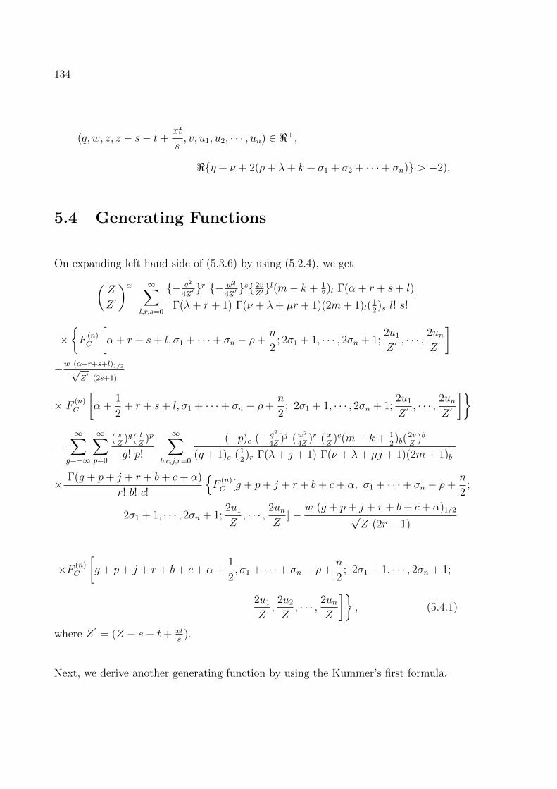
134

(q, w, z, z − s− t+xt

s, v, u1, u2, · · · , un) ∈ <+,

<η + ν + 2(ρ+ λ+ k + σ1 + σ2 + · · ·+ σn) > −2).

5.4 Generating Functions

On expanding left hand side of (5.3.6) by using (5.2.4), we get(Z

Z ′

)α ∞∑l,r,s=0

− q2

4Z′r − w2

4Z′s 2v

Z′l(m− k + 1

2)l Γ(α + r + s+ l)

Γ(λ+ r + 1) Γ(ν + λ+ µr + 1)(2m+ 1)l(12)s l! s!

×F

(n)C

[α + r + s+ l, σ1 + · · ·+ σn − ρ+

n

2; 2σ1 + 1, · · · , 2σn + 1;

2u1

Z ′, · · · , 2un

Z ′

]−w (α+r+s+l)1/2√

Z′ (2s+1)

× F (n)C

[α +

1

2+ r + s+ l, σ1 + · · ·+ σn − ρ+

n

2; 2σ1 + 1, · · · , 2σn + 1;

2u1

Z ′, · · · , 2un

Z ′

]

=∞∑

g=−∞

∞∑p=0

( sZ

)g( tZ

)p

g! p!

∞∑b,c,j,r=0

(−p)c (− q2

4Z)j (w

2

4Z)r ( x

Z)c(m− k + 1

2)b(

2vZ

)b

(g + 1)c (12)r Γ(λ+ j + 1) Γ(ν + λ+ µj + 1)(2m+ 1)b

× Γ(g + p+ j + r + b+ c+ α)

r! b! c!

F

(n)C [g + p+ j + r + b+ c+ α, σ1 + · · ·+ σn − ρ+

n

2;

2σ1 + 1, · · · , 2σn + 1;2u1

Z, · · · , 2un

Z] −

w (g + p+ j + r + b+ c+ α)1/2√Z (2r + 1)

×F (n)C

[g + p+ j + r + b+ c+ α +

1

2, σ1 + · · ·+ σn − ρ+

n

2; 2σ1 + 1, · · · , 2σn + 1;

2u1

Z,2u2

Z, · · · , 2un

Z

], (5.4.1)

where Z′= (Z − s− t+ xt

s).

Next, we derive another generating function by using the Kummer’s first formula.

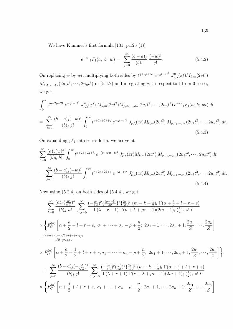
135

We have Kummer’s first formula [131; p.125 (1)]

e−w 1F1(a; b; w) =∞∑j=0

(b− a)j(b)j

(−w)j

j!. (5.4.2)

On replacing w by wt, multiplying both sides by tη+2ρ+2k e−yt−zt2Jµν,λ(xt)Mk,m(2vt2)

Mρ,σ1,···,σn(2u1t2, · · · , 2unt2) in (5.4.2) and integrating with respect to t from 0 to ∞,

we get∫ ∞0

tη+2ρ+2k e−yt−zt2

Jµν,λ(xt)Mk,m(2vt2)Mρ,σ1,···,σn(2u1t2, · · · , 2unt2) e−wt1F1(a; b; wt) dt

=∞∑j=0

(b− a)j(−w)j

(b)j j!

∫ ∞0

tη+2ρ+2k+j e−yt−zt2

Jµν,λ(xt)Mk,m(2vt2)Mρ,σ1,···,σn(2u1t2, · · · , 2unt2) dt.

(5.4.3)

On expanding 1F1 into series form, we arrive at

∞∑h=0

(a)h(w)h

(b)h h!

∫ ∞0

tη+2ρ+2k+h e−(y+w)t−zt2 Jµν,λ(xt)Mk,m(2vt2)Mρ,σ1,···,σn(2u1t2, · · · , 2unt2) dt

=∞∑j=0

(b− a)j(−w)j

(b)j j!

∫ ∞0

tη+2ρ+2k+j e−yt−zt2

Jµν,λ(xt)Mk,m(2vt2)Mρ,σ1,···,σn(2u1t2, · · · , 2unt2) dt.

(5.4.4)

Now using (5.2.4) on both sides of (5.4.4), we get

∞∑h=0

(a)h(w√Z

)h

(b)h h!

∞∑l,r,s=0

(− x2

4Z)r (y+w)2

4Zs2v

Zl (m− k + 1

2)l Γ(α + h

2+ l + r + s)

Γ(λ+ r + 1) Γ(ν + λ+ µr + 1)(2m+ 1)l (12)s s! l!

×F

(n)C

[α +

h

2+ l + r + s, σ1 + · · ·+ σn − ρ+

n

2; 2σ1 + 1, · · · , 2σn + 1;

2u1

Z, · · · , 2un

Z

]− (y+w) (α+h/2+l+r+s)1/2√

Z (2s+1)

× F (n)C

[α +

h

2+

1

2+ l + r + s, σ1 + · · ·+ σn − ρ+

n

2; 2σ1 + 1, · · · , 2σn + 1;

2u1

Z, · · · , 2un

Z

]

=∞∑j=0

(b− a)j(− w√Z

)j

(b)j j!

∞∑l,r,s=0

(− x2

4Z)r( y

2

4Z)s2v

Zl (m− k + 1

2)l Γ(α + d

2+ l + r + s)

Γ(λ+ r + 1) Γ(ν + λ+ µr + 1)(2m+ 1)l (12)s s! l!

×F

(n)C

[α +

j

2+ l + r + s, σ1 + · · ·+ σn − ρ+

n

2; 2σ1 + 1, · · · , 2σn + 1;

2u1

Z, · · · , 2un

Z

]

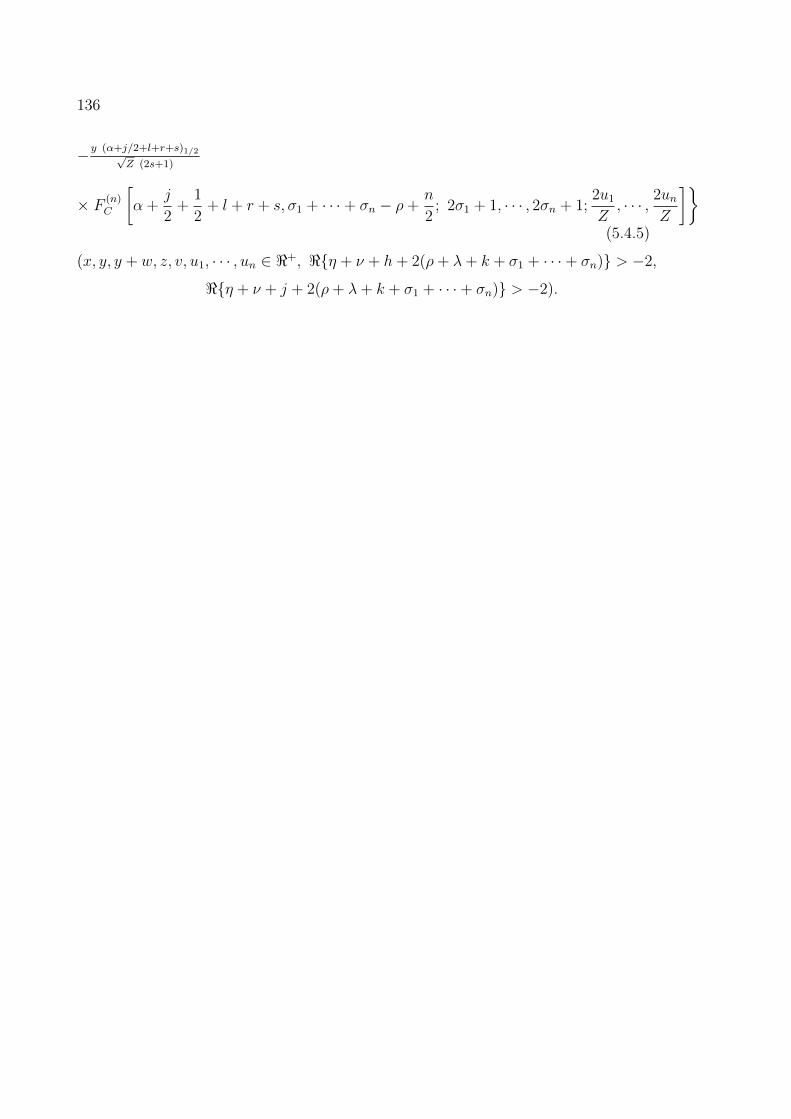
136

−y (α+j/2+l+r+s)1/2√Z (2s+1)

× F (n)C

[α +

j

2+

1

2+ l + r + s, σ1 + · · ·+ σn − ρ+

n

2; 2σ1 + 1, · · · , 2σn + 1;

2u1

Z, · · · , 2un

Z

](5.4.5)

(x, y, y + w, z, v, u1, · · · , un ∈ <+, <η + ν + h+ 2(ρ+ λ+ k + σ1 + · · ·+ σn) > −2,

<η + ν + j + 2(ρ+ λ+ k + σ1 + · · ·+ σn) > −2).

Chapter 6

On Certain Integral FormulasInvolving the Product of BesselFunction and Jacobi Polynomial

6.1 Introduction

Some very interesting integrals associated with a variety of special functions have

been established by many authors (see, [4], [10], [24], [30], [31]). Very recently, Choi

and Agarwal [22] gave some interesting unified integrals involving the Bessel function

of the first kind, which are expressed in terms of generalized (Wright) hypergeometric

function.

Motivated by the above-mentioned works, in the present chapter, we have es-

tablished a new class of integral formulas involving the product of Bessel function

Jν(z) with Jacobi polynomial P(α,β)n (z), which are expressed in terms of Kampe de

Feriet and Srivastava and Daoust functions. Some other integrals involving the prod-

uct of Bessel (sine and cosine) function with ultraspherical polynomial, Gegenbauer

polynomial, Tchebicheff polynomial, and Legendre polynomial are also established

as special cases of our main results. Next, we have established a very interesting

connection between Kampe de Feriet function and Srivastava and Daoust function.

The main object of the present chapter is to obtain certain integral formulas

involving the product of Bessel function of the first kind and Jacobi polynomial,

137

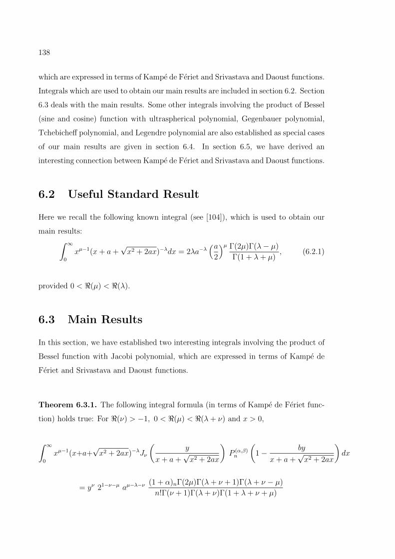
138

which are expressed in terms of Kampe de Feriet and Srivastava and Daoust functions.

Integrals which are used to obtain our main results are included in section 6.2. Section

6.3 deals with the main results. Some other integrals involving the product of Bessel

(sine and cosine) function with ultraspherical polynomial, Gegenbauer polynomial,

Tchebicheff polynomial, and Legendre polynomial are also established as special cases

of our main results are given in section 6.4. In section 6.5, we have derived an

interesting connection between Kampe de Feriet and Srivastava and Daoust functions.

6.2 Useful Standard Result

Here we recall the following known integral (see [104]), which is used to obtain our

main results:∫ ∞0

xµ−1(x+ a+√x2 + 2ax)−λdx = 2λa−λ

(a2

)µ Γ(2µ)Γ(λ− µ)

Γ(1 + λ+ µ), (6.2.1)

provided 0 < <(µ) < <(λ).

6.3 Main Results

In this section, we have established two interesting integrals involving the product of

Bessel function with Jacobi polynomial, which are expressed in terms of Kampe de

Feriet and Srivastava and Daoust functions.

Theorem 6.3.1. The following integral formula (in terms of Kampe de Feriet func-

tion) holds true: For <(ν) > −1, 0 < <(µ) < <(λ+ ν) and x > 0,

∫ ∞0

xµ−1(x+a+√x2 + 2ax)−λJν

(y

x+ a+√x2 + 2ax

)P (α,β)n

(1− by

x+ a+√x2 + 2ax

)dx

= yν 21−ν−µ aµ−λ−ν(1 + α)nΓ(2µ)Γ(λ+ ν + 1)Γ(λ+ ν − µ)

n!Γ(ν + 1)Γ(λ+ ν)Γ(1 + λ+ ν + µ)

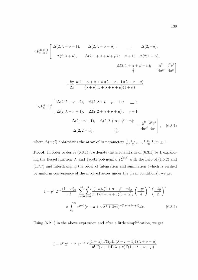
139

×F 4: 0; 44: 1; 3

∆(2;λ+ ν + 1), ∆(2;λ+ ν − µ) : ; ∆(2;−n),

∆(2;λ+ ν), ∆(2; 1 + λ+ ν + µ) : ν + 1; ∆(2; 1 + α),

∆(2; 1 + α + β + n);12;

− y2

4a2,b2y2

4a2

]

+by

2a

n(1 + α + β + n)(λ+ ν + 1)(λ+ ν − µ)

(λ+ ν)(1 + λ+ ν + µ)(1 + α)

×F 4: 0; 44: 1; 3

∆(2;λ+ ν + 2), ∆(2;λ+ ν − µ+ 1) : ;

∆(2;λ+ ν + 1), ∆(2; 2 + λ+ ν + µ) : ν + 1;

∆(2;−n+ 1), ∆(2; 2 + α + β + n);

∆(2; 2 + α), 32;

− y2

4a2,b2y2

4a2

, (6.3.1)

where ∆(m; l) abbreviates the array of m parameters lm, l+1m, ...., l+m−1

m,m ≥ 1.

Proof: In order to derive (6.3.1), we denote the left-hand side of (6.3.1) by I, expand-

ing the Bessel function Jν and Jacobi polynomial P(α,β)n with the help of (1.5.2) and

(1.7.7) and interchanging the order of integration and summation (which is verified

by uniform convergence of the involved series under the given conditions), we get

I = yν 2−ν(1 + α)n

n!

∞∑m=0

n∑k=0

(−n)k(1 + α + β + n)km!Γ(ν +m+ 1)(1 + α)k

(−y2

4

)m(−by2

)k

×∫ ∞

0

xµ−1(x+ a+√x2 + 2ax)−(λ+ν+2m+k)dx. (6.3.2)

Using (6.2.1) in the above expression and after a little simplification, we get

I = yν 21−ν−µ aµ−λ−ν(1 + α)nΓ(2µ)Γ(λ+ ν + 1)Γ(λ+ ν − µ)

n! Γ(ν + 1)Γ(λ+ ν)Γ(1 + λ+ ν + µ)

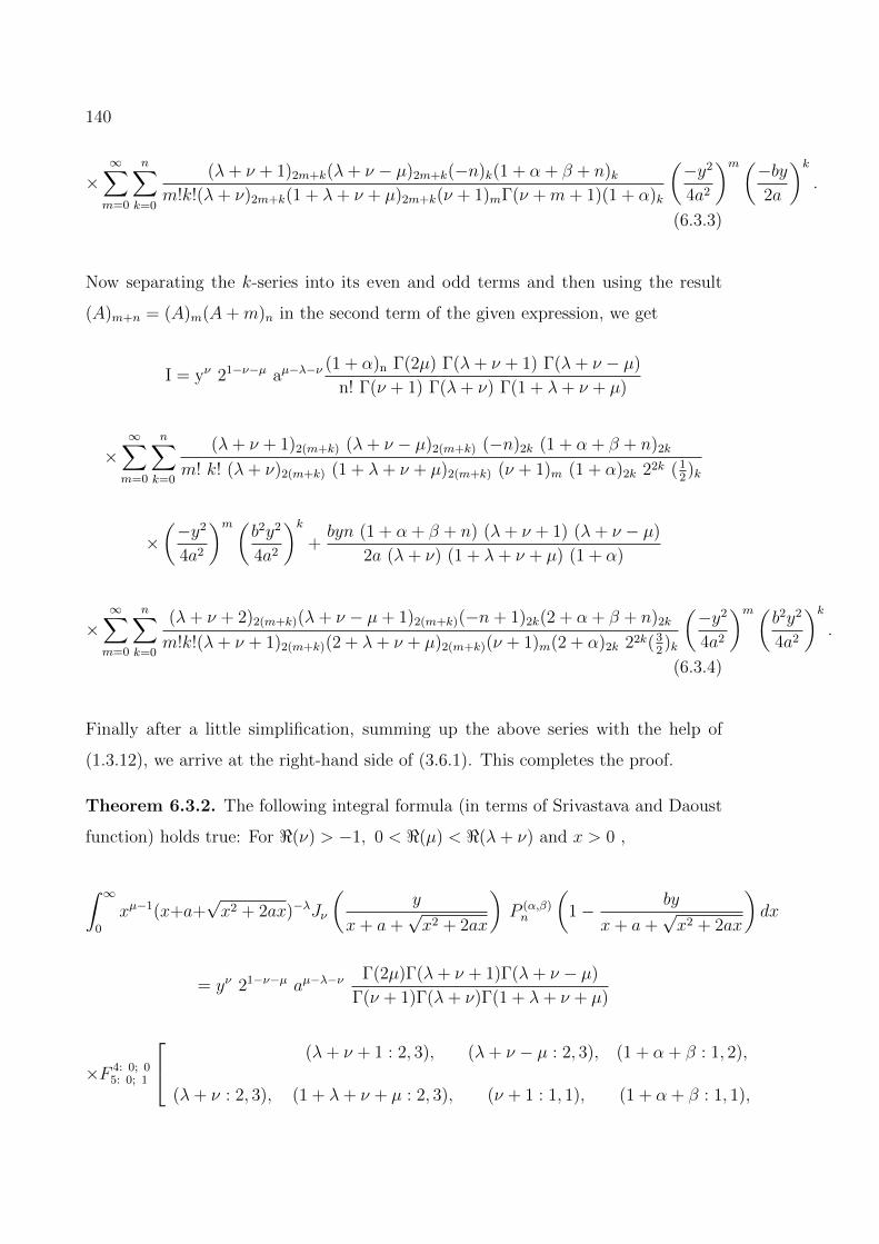
140

×∞∑m=0

n∑k=0

(λ+ ν + 1)2m+k(λ+ ν − µ)2m+k(−n)k(1 + α + β + n)km!k!(λ+ ν)2m+k(1 + λ+ ν + µ)2m+k(ν + 1)mΓ(ν +m+ 1)(1 + α)k

(−y2

4a2

)m(−by2a

)k.

(6.3.3)

Now separating the k-series into its even and odd terms and then using the result

(A)m+n = (A)m(A+m)n in the second term of the given expression, we get

I = yν 21−ν−µ aµ−λ−ν(1 + α)n Γ(2µ) Γ(λ+ ν + 1) Γ(λ+ ν − µ)

n! Γ(ν + 1) Γ(λ+ ν) Γ(1 + λ+ ν + µ)

×∞∑m=0

n∑k=0

(λ+ ν + 1)2(m+k) (λ+ ν − µ)2(m+k) (−n)2k (1 + α + β + n)2k

m! k! (λ+ ν)2(m+k) (1 + λ+ ν + µ)2(m+k) (ν + 1)m (1 + α)2k 22k (12)k

×(−y2

4a2

)m(b2y2

4a2

)k+byn (1 + α + β + n) (λ+ ν + 1) (λ+ ν − µ)

2a (λ+ ν) (1 + λ+ ν + µ) (1 + α)

×∞∑m=0

n∑k=0

(λ+ ν + 2)2(m+k)(λ+ ν − µ+ 1)2(m+k)(−n+ 1)2k(2 + α + β + n)2k

m!k!(λ+ ν + 1)2(m+k)(2 + λ+ ν + µ)2(m+k)(ν + 1)m(2 + α)2k 22k(32)k

(−y2

4a2

)m(b2y2

4a2

)k.

(6.3.4)

Finally after a little simplification, summing up the above series with the help of

(1.3.12), we arrive at the right-hand side of (3.6.1). This completes the proof.

Theorem 6.3.2. The following integral formula (in terms of Srivastava and Daoust

function) holds true: For <(ν) > −1, 0 < <(µ) < <(λ+ ν) and x > 0 ,

∫ ∞0

xµ−1(x+a+√x2 + 2ax)−λJν

(y

x+ a+√x2 + 2ax

)P (α,β)n

(1− by

x+ a+√x2 + 2ax

)dx

= yν 21−ν−µ aµ−λ−νΓ(2µ)Γ(λ+ ν + 1)Γ(λ+ ν − µ)

Γ(ν + 1)Γ(λ+ ν)Γ(1 + λ+ ν + µ)

×F 4: 0; 05: 0; 1

(λ+ ν + 1 : 2, 3), (λ+ ν − µ : 2, 3), (1 + α + β : 1, 2),

(λ+ ν : 2, 3), (1 + λ+ ν + µ : 2, 3), (ν + 1 : 1, 1), (1 + α + β : 1, 1),

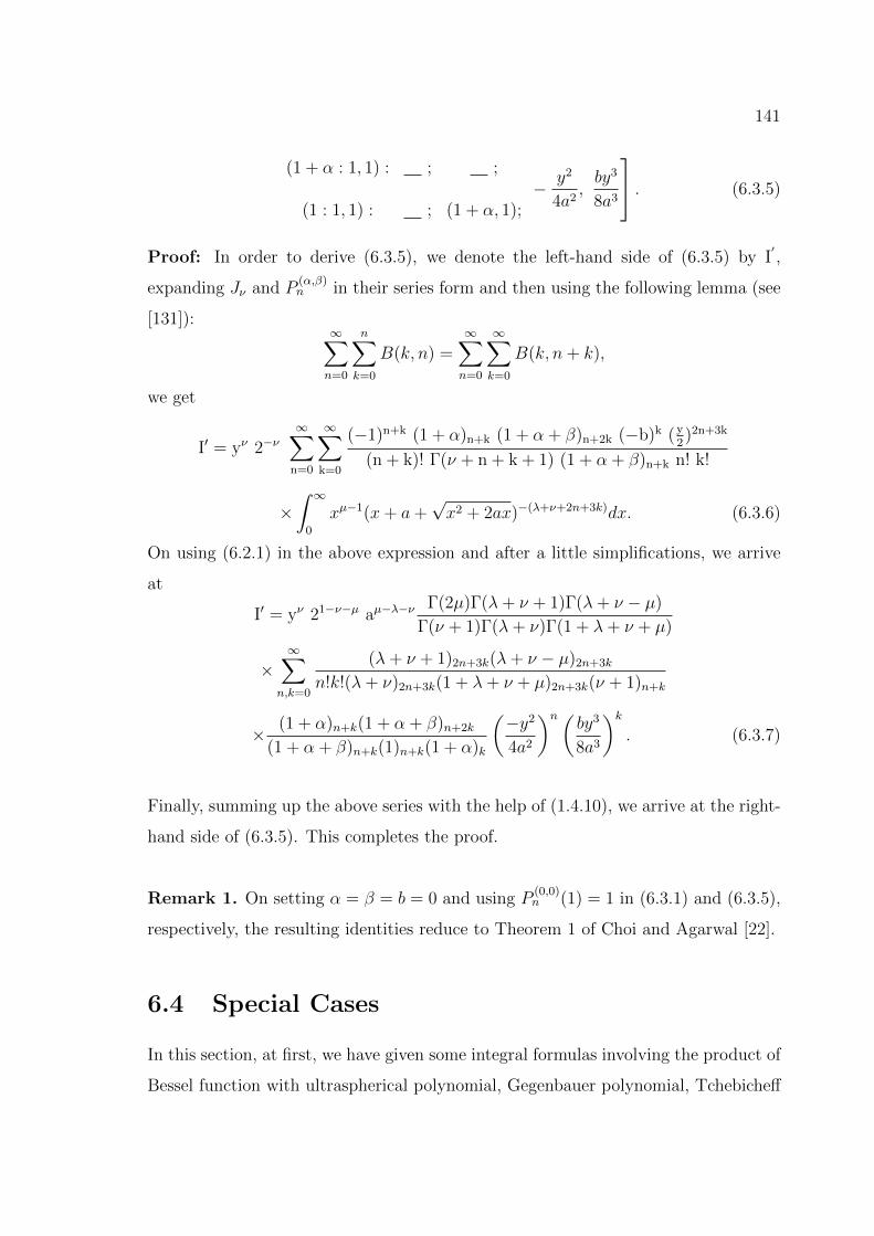
141

(1 + α : 1, 1) : ; ;

(1 : 1, 1) : ; (1 + α, 1);− y2

4a2,by3

8a3

. (6.3.5)

Proof: In order to derive (6.3.5), we denote the left-hand side of (6.3.5) by I′,

expanding Jν and P(α,β)n in their series form and then using the following lemma (see

[131]):∞∑n=0

n∑k=0

B(k, n) =∞∑n=0

∞∑k=0

B(k, n+ k),

we get

I′ = yν 2−ν∞∑

n=0

∞∑k=0

(−1)n+k (1 + α)n+k (1 + α + β)n+2k (−b)k (y2)2n+3k

(n + k)! Γ(ν + n + k + 1) (1 + α + β)n+k n! k!

×∫ ∞

0

xµ−1(x+ a+√x2 + 2ax)−(λ+ν+2n+3k)dx. (6.3.6)

On using (6.2.1) in the above expression and after a little simplifications, we arrive

at

I′ = yν 21−ν−µ aµ−λ−νΓ(2µ)Γ(λ+ ν + 1)Γ(λ+ ν − µ)

Γ(ν + 1)Γ(λ+ ν)Γ(1 + λ+ ν + µ)

×∞∑

n,k=0

(λ+ ν + 1)2n+3k(λ+ ν − µ)2n+3k

n!k!(λ+ ν)2n+3k(1 + λ+ ν + µ)2n+3k(ν + 1)n+k

× (1 + α)n+k(1 + α + β)n+2k

(1 + α + β)n+k(1)n+k(1 + α)k

(−y2

4a2

)n(by3

8a3

)k. (6.3.7)

Finally, summing up the above series with the help of (1.4.10), we arrive at the right-

hand side of (6.3.5). This completes the proof.

Remark 1. On setting α = β = b = 0 and using P(0,0)n (1) = 1 in (6.3.1) and (6.3.5),

respectively, the resulting identities reduce to Theorem 1 of Choi and Agarwal [22].

6.4 Special Cases

In this section, at first, we have given some integral formulas involving the product of

Bessel function with ultraspherical polynomial, Gegenbauer polynomial, Tchebicheff

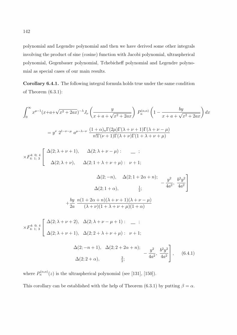
142

polynomial and Legendre polynomial and then we have derived some other integrals

involving the product of sine (cosine) function with Jacobi polynomial, ultraspherical

polynomial, Gegenbauer polynomial, Tchebicheff polynomial and Legendre polyno-

mial as special cases of our main results.

Corollary 6.4.1. The following integral formula holds true under the same condition

of Theorem (6.3.1):

∫ ∞0

xµ−1(x+a+√x2 + 2ax)−λJν

(y

x+ a+√x2 + 2ax

)P (α,α)n

(1− by

x+ a+√x2 + 2ax

)dx

= yν 21−ν−µ aµ−λ−ν(1 + α)nΓ(2µ)Γ(λ+ ν + 1)Γ(λ+ ν − µ)

n!Γ(ν + 1)Γ(λ+ ν)Γ(1 + λ+ ν + µ)

×F 4: 0; 44: 1; 3

∆(2;λ+ ν + 1), ∆(2;λ+ ν − µ) : ;

∆(2;λ+ ν), ∆(2; 1 + λ+ ν + µ) : ν + 1;

∆(2;−n), ∆(2; 1 + 2α + n);

∆(2; 1 + α), 12;

− y2

4a2,b2y2

4a2

+by

2a

n(1 + 2α + n)(λ+ ν + 1)(λ+ ν − µ)

(λ+ ν)(1 + λ+ ν + µ)(1 + α)

×F 4: 0; 44: 1; 3

∆(2;λ+ ν + 2), ∆(2;λ+ ν − µ+ 1) : ;

∆(2;λ+ ν + 1), ∆(2; 2 + λ+ ν + µ) : ν + 1;

∆(2;−n+ 1), ∆(2; 2 + 2α + n);

∆(2; 2 + α), 32;

− y2

4a2,b2y2

4a2

, (6.4.1)

where P(α,α)n (z) is the ultraspherical polynomial (see [131], [150]).

This corollary can be established with the help of Theorem (6.3.1) by putting β = α.

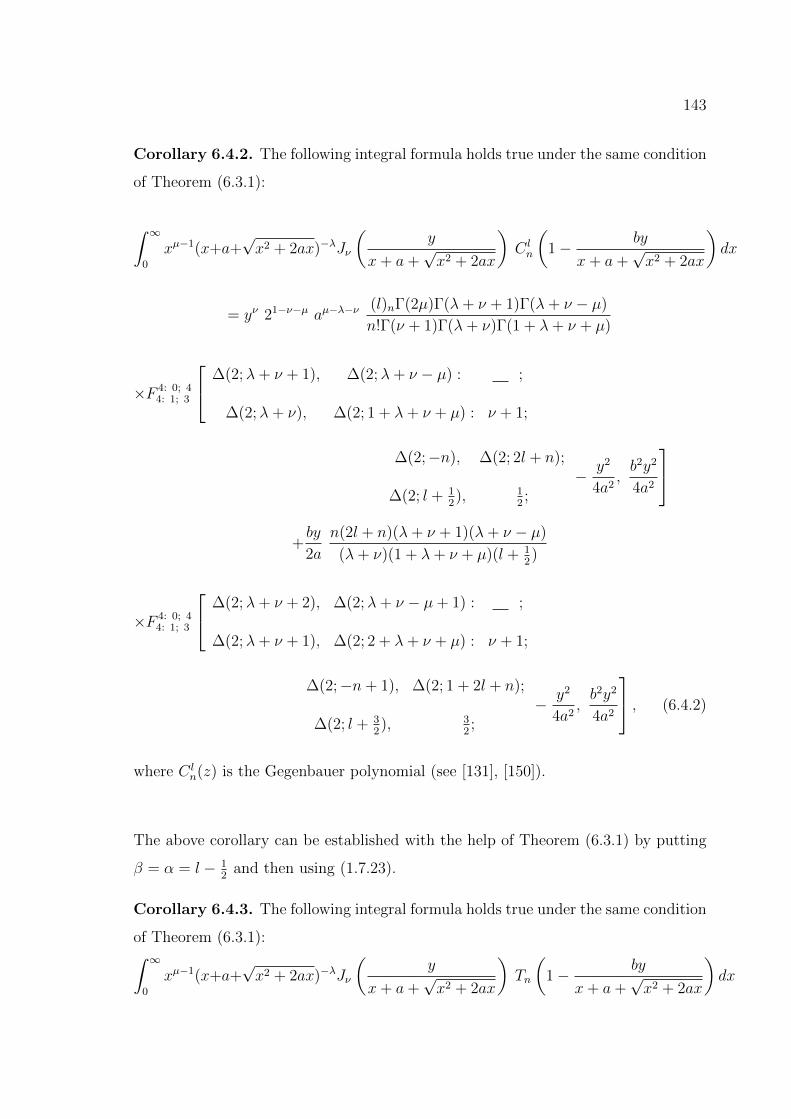
143

Corollary 6.4.2. The following integral formula holds true under the same condition

of Theorem (6.3.1):

∫ ∞0

xµ−1(x+a+√x2 + 2ax)−λJν

(y

x+ a+√x2 + 2ax

)C ln

(1− by

x+ a+√x2 + 2ax

)dx

= yν 21−ν−µ aµ−λ−ν(l)nΓ(2µ)Γ(λ+ ν + 1)Γ(λ+ ν − µ)

n!Γ(ν + 1)Γ(λ+ ν)Γ(1 + λ+ ν + µ)

×F 4: 0; 44: 1; 3

∆(2;λ+ ν + 1), ∆(2;λ+ ν − µ) : ;

∆(2;λ+ ν), ∆(2; 1 + λ+ ν + µ) : ν + 1;

∆(2;−n), ∆(2; 2l + n);

∆(2; l + 12), 1

2;

− y2

4a2,b2y2

4a2

+by

2a

n(2l + n)(λ+ ν + 1)(λ+ ν − µ)

(λ+ ν)(1 + λ+ ν + µ)(l + 12)

×F 4: 0; 44: 1; 3

∆(2;λ+ ν + 2), ∆(2;λ+ ν − µ+ 1) : ;

∆(2;λ+ ν + 1), ∆(2; 2 + λ+ ν + µ) : ν + 1;

∆(2;−n+ 1), ∆(2; 1 + 2l + n);

∆(2; l + 32), 3

2;

− y2

4a2,b2y2

4a2

, (6.4.2)

where C ln(z) is the Gegenbauer polynomial (see [131], [150]).

The above corollary can be established with the help of Theorem (6.3.1) by putting

β = α = l − 12

and then using (1.7.23).

Corollary 6.4.3. The following integral formula holds true under the same condition

of Theorem (6.3.1):∫ ∞0

xµ−1(x+a+√x2 + 2ax)−λJν

(y

x+ a+√x2 + 2ax

)Tn

(1− by

x+ a+√x2 + 2ax

)dx

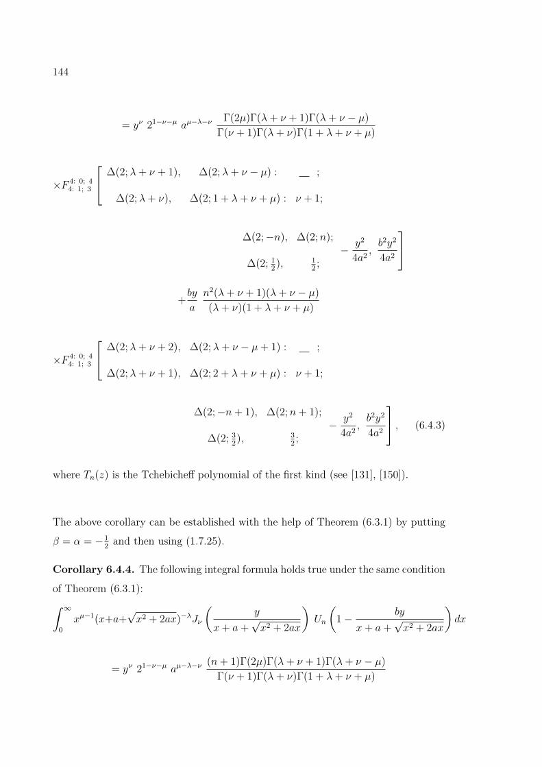
144

= yν 21−ν−µ aµ−λ−νΓ(2µ)Γ(λ+ ν + 1)Γ(λ+ ν − µ)

Γ(ν + 1)Γ(λ+ ν)Γ(1 + λ+ ν + µ)

×F 4: 0; 44: 1; 3

∆(2;λ+ ν + 1), ∆(2;λ+ ν − µ) : ;

∆(2;λ+ ν), ∆(2; 1 + λ+ ν + µ) : ν + 1;

∆(2;−n), ∆(2;n);

∆(2; 12), 1

2;

− y2

4a2,b2y2

4a2

+by

a

n2(λ+ ν + 1)(λ+ ν − µ)

(λ+ ν)(1 + λ+ ν + µ)

×F 4: 0; 44: 1; 3

∆(2;λ+ ν + 2), ∆(2;λ+ ν − µ+ 1) : ;

∆(2;λ+ ν + 1), ∆(2; 2 + λ+ ν + µ) : ν + 1;

∆(2;−n+ 1), ∆(2;n+ 1);

∆(2; 32), 3

2;

− y2

4a2,b2y2

4a2

, (6.4.3)

where Tn(z) is the Tchebicheff polynomial of the first kind (see [131], [150]).

The above corollary can be established with the help of Theorem (6.3.1) by putting

β = α = −12

and then using (1.7.25).

Corollary 6.4.4. The following integral formula holds true under the same condition

of Theorem (6.3.1):∫ ∞0

xµ−1(x+a+√x2 + 2ax)−λJν

(y

x+ a+√x2 + 2ax

)Un

(1− by

x+ a+√x2 + 2ax

)dx

= yν 21−ν−µ aµ−λ−ν(n+ 1)Γ(2µ)Γ(λ+ ν + 1)Γ(λ+ ν − µ)

Γ(ν + 1)Γ(λ+ ν)Γ(1 + λ+ ν + µ)

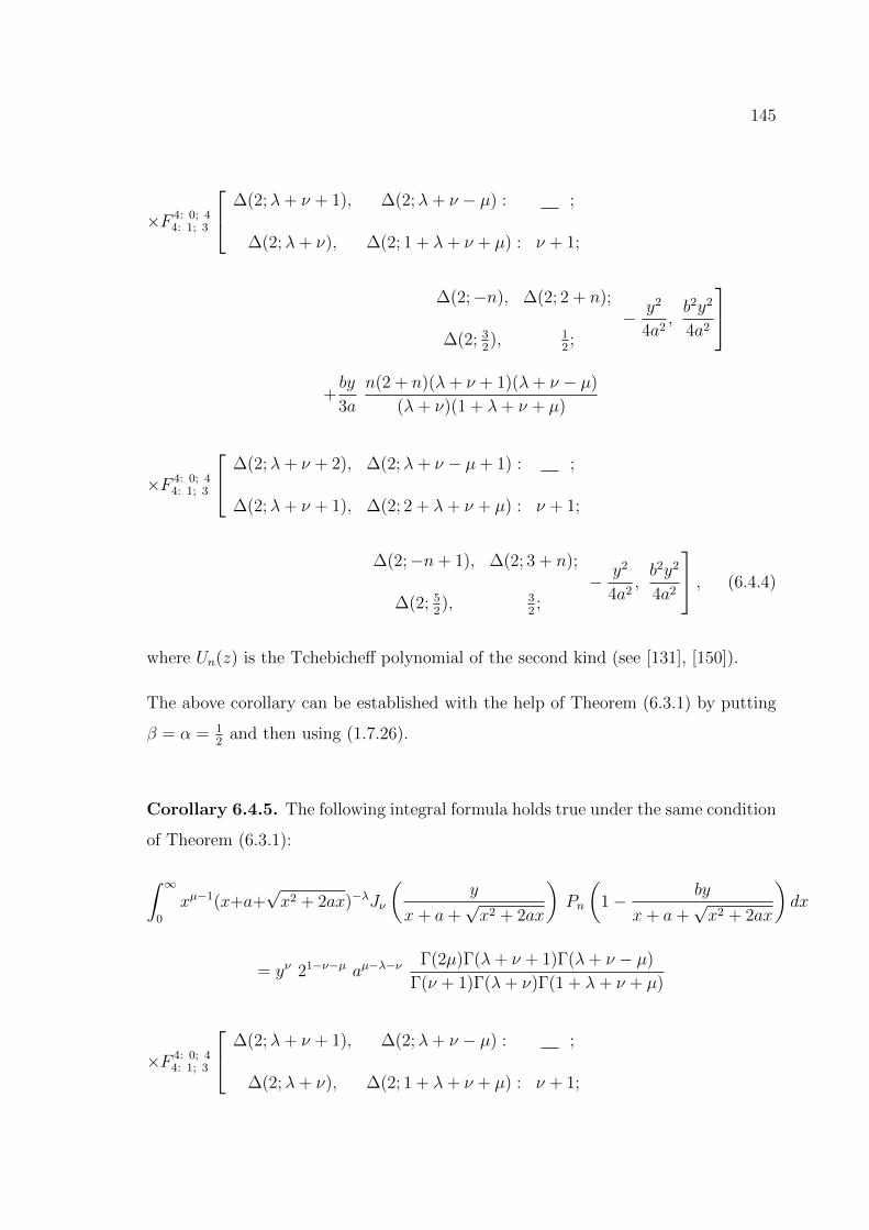
145

×F 4: 0; 44: 1; 3

∆(2;λ+ ν + 1), ∆(2;λ+ ν − µ) : ;

∆(2;λ+ ν), ∆(2; 1 + λ+ ν + µ) : ν + 1;

∆(2;−n), ∆(2; 2 + n);

∆(2; 32), 1

2;

− y2

4a2,b2y2

4a2

+by

3a

n(2 + n)(λ+ ν + 1)(λ+ ν − µ)

(λ+ ν)(1 + λ+ ν + µ)

×F 4: 0; 44: 1; 3

∆(2;λ+ ν + 2), ∆(2;λ+ ν − µ+ 1) : ;

∆(2;λ+ ν + 1), ∆(2; 2 + λ+ ν + µ) : ν + 1;

∆(2;−n+ 1), ∆(2; 3 + n);

∆(2; 52), 3

2;

− y2

4a2,b2y2

4a2

, (6.4.4)

where Un(z) is the Tchebicheff polynomial of the second kind (see [131], [150]).

The above corollary can be established with the help of Theorem (6.3.1) by putting

β = α = 12

and then using (1.7.26).

Corollary 6.4.5. The following integral formula holds true under the same condition

of Theorem (6.3.1):

∫ ∞0

xµ−1(x+a+√x2 + 2ax)−λJν

(y

x+ a+√x2 + 2ax

)Pn

(1− by

x+ a+√x2 + 2ax

)dx

= yν 21−ν−µ aµ−λ−νΓ(2µ)Γ(λ+ ν + 1)Γ(λ+ ν − µ)

Γ(ν + 1)Γ(λ+ ν)Γ(1 + λ+ ν + µ)

×F 4: 0; 44: 1; 3

∆(2;λ+ ν + 1), ∆(2;λ+ ν − µ) : ;

∆(2;λ+ ν), ∆(2; 1 + λ+ ν + µ) : ν + 1;

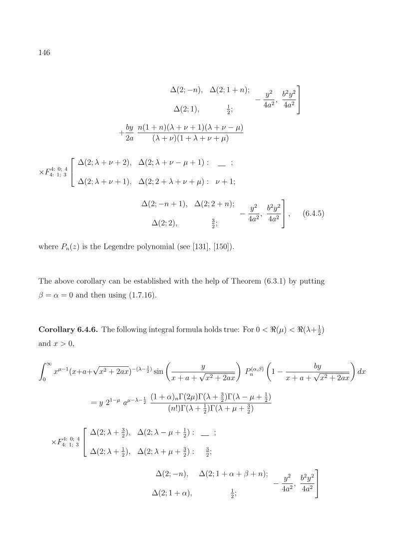
146

∆(2;−n), ∆(2; 1 + n);

∆(2; 1), 12;

− y2

4a2,b2y2

4a2

+by

2a

n(1 + n)(λ+ ν + 1)(λ+ ν − µ)

(λ+ ν)(1 + λ+ ν + µ)

×F 4: 0; 44: 1; 3

∆(2;λ+ ν + 2), ∆(2;λ+ ν − µ+ 1) : ;

∆(2;λ+ ν + 1), ∆(2; 2 + λ+ ν + µ) : ν + 1;

∆(2;−n+ 1), ∆(2; 2 + n);

∆(2; 2), 32;

− y2

4a2,b2y2

4a2

, (6.4.5)

where Pn(z) is the Legendre polynomial (see [131], [150]).

The above corollary can be established with the help of Theorem (6.3.1) by putting

β = α = 0 and then using (1.7.16).

Corollary 6.4.6. The following integral formula holds true: For 0 < <(µ) < <(λ+ 12)

and x > 0,

∫ ∞0

xµ−1(x+a+√x2 + 2ax)−(λ− 1

2) sin

(y

x+ a+√x2 + 2ax

)P (α,β)n

(1− by

x+ a+√x2 + 2ax

)dx

= y 21−µ aµ−λ−12

(1 + α)nΓ(2µ)Γ(λ+ 32)Γ(λ− µ+ 1

2)

(n!)Γ(λ+ 12)Γ(λ+ µ+ 3

2)

×F 4: 0; 44: 1; 3

∆(2;λ+ 32), ∆(2;λ− µ+ 1

2) : ;

∆(2;λ+ 12), ∆(2;λ+ µ+ 3

2) : 3

2;

∆(2;−n), ∆(2; 1 + α + β + n);

∆(2; 1 + α), 12;

− y2

4a2,b2y2

4a2

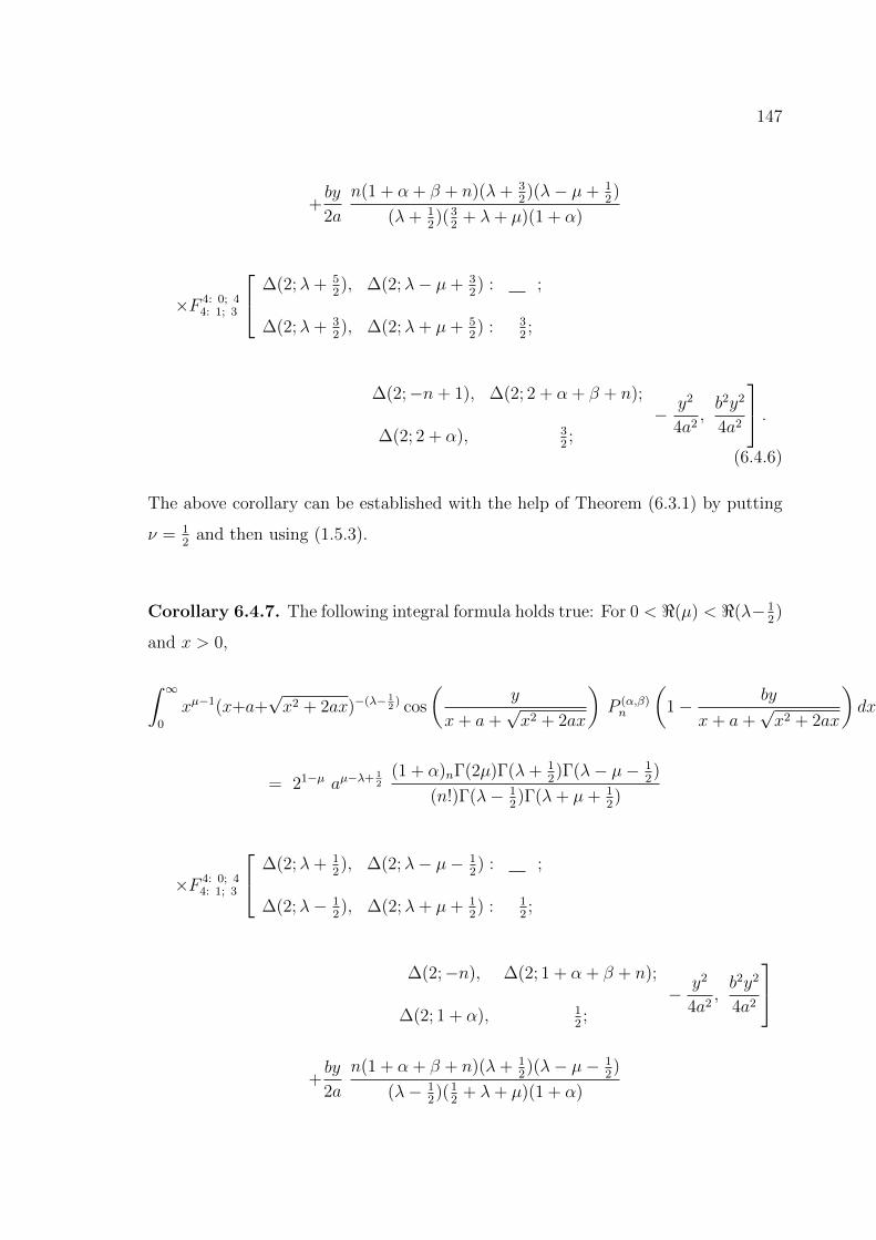
147

+by

2a

n(1 + α + β + n)(λ+ 32)(λ− µ+ 1

2)

(λ+ 12)(3

2+ λ+ µ)(1 + α)

×F 4: 0; 44: 1; 3

∆(2;λ+ 52), ∆(2;λ− µ+ 3

2) : ;

∆(2;λ+ 32), ∆(2;λ+ µ+ 5

2) : 3

2;

∆(2;−n+ 1), ∆(2; 2 + α + β + n);

∆(2; 2 + α), 32;

− y2

4a2,b2y2

4a2

.(6.4.6)

The above corollary can be established with the help of Theorem (6.3.1) by putting

ν = 12

and then using (1.5.3).

Corollary 6.4.7. The following integral formula holds true: For 0 < <(µ) < <(λ− 12)

and x > 0,

∫ ∞0

xµ−1(x+a+√x2 + 2ax)−(λ− 1

2) cos

(y

x+ a+√x2 + 2ax

)P (α,β)n

(1− by

x+ a+√x2 + 2ax

)dx

= 21−µ aµ−λ+ 12

(1 + α)nΓ(2µ)Γ(λ+ 12)Γ(λ− µ− 1

2)

(n!)Γ(λ− 12)Γ(λ+ µ+ 1

2)

×F 4: 0; 44: 1; 3

∆(2;λ+ 12), ∆(2;λ− µ− 1

2) : ;

∆(2;λ− 12), ∆(2;λ+ µ+ 1

2) : 1

2;

∆(2;−n), ∆(2; 1 + α + β + n);

∆(2; 1 + α), 12;

− y2

4a2,b2y2

4a2

+by

2a

n(1 + α + β + n)(λ+ 12)(λ− µ− 1

2)

(λ− 12)(1

2+ λ+ µ)(1 + α)

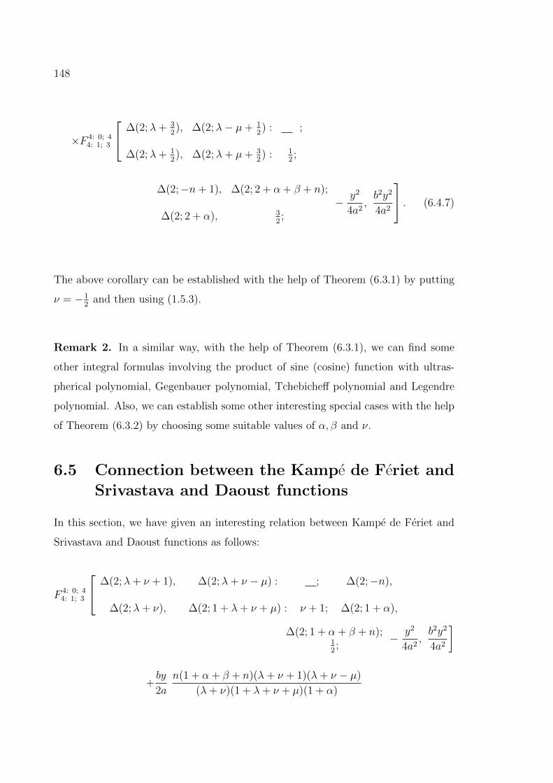
148

×F 4: 0; 44: 1; 3

∆(2;λ+ 32), ∆(2;λ− µ+ 1

2) : ;

∆(2;λ+ 12), ∆(2;λ+ µ+ 3

2) : 1

2;

∆(2;−n+ 1), ∆(2; 2 + α + β + n);

∆(2; 2 + α), 32;

− y2

4a2,b2y2

4a2

. (6.4.7)

The above corollary can be established with the help of Theorem (6.3.1) by putting

ν = −12

and then using (1.5.3).

Remark 2. In a similar way, with the help of Theorem (6.3.1), we can find some

other integral formulas involving the product of sine (cosine) function with ultras-

pherical polynomial, Gegenbauer polynomial, Tchebicheff polynomial and Legendre

polynomial. Also, we can establish some other interesting special cases with the help

of Theorem (6.3.2) by choosing some suitable values of α, β and ν.

6.5 Connection between the Kampe de Feriet and

Srivastava and Daoust functions

In this section, we have given an interesting relation between Kampe de Feriet and

Srivastava and Daoust functions as follows:

F 4: 0; 44: 1; 3

∆(2;λ+ ν + 1), ∆(2;λ+ ν − µ) : ; ∆(2;−n),

∆(2;λ+ ν), ∆(2; 1 + λ+ ν + µ) : ν + 1; ∆(2; 1 + α),

∆(2; 1 + α + β + n);12;

− y2

4a2,b2y2

4a2

]

+by

2a

n(1 + α + β + n)(λ+ ν + 1)(λ+ ν − µ)

(λ+ ν)(1 + λ+ ν + µ)(1 + α)

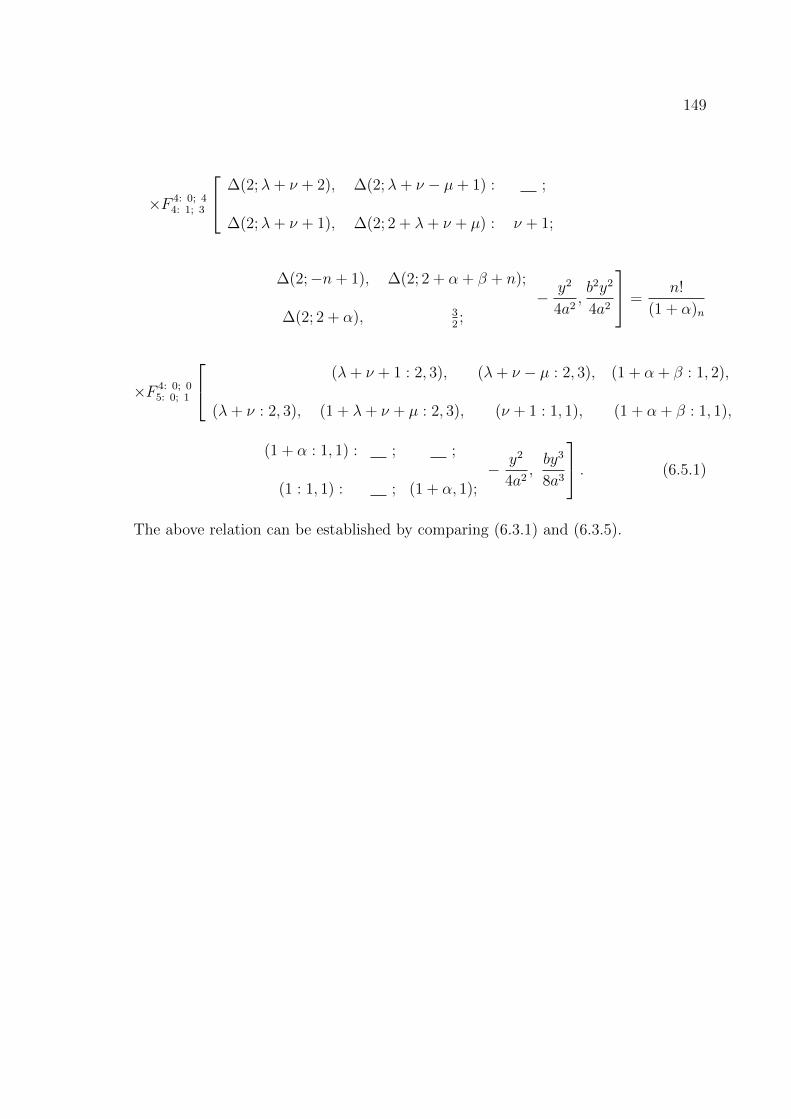
149

×F 4: 0; 44: 1; 3

∆(2;λ+ ν + 2), ∆(2;λ+ ν − µ+ 1) : ;

∆(2;λ+ ν + 1), ∆(2; 2 + λ+ ν + µ) : ν + 1;

∆(2;−n+ 1), ∆(2; 2 + α + β + n);

∆(2; 2 + α), 32;

− y2

4a2,b2y2

4a2

=n!

(1 + α)n

×F 4: 0; 05: 0; 1

(λ+ ν + 1 : 2, 3), (λ+ ν − µ : 2, 3), (1 + α + β : 1, 2),

(λ+ ν : 2, 3), (1 + λ+ ν + µ : 2, 3), (ν + 1 : 1, 1), (1 + α + β : 1, 1),

(1 + α : 1, 1) : ; ;

(1 : 1, 1) : ; (1 + α, 1);− y2

4a2,by3

8a3

. (6.5.1)

The above relation can be established by comparing (6.3.1) and (6.3.5).

Chapter 7

Integral Transforms Associatedwith Whittaker and BesselFunction

7.1 Introduction

Integral transformations have been successfully used for almost two centuries in solv-

ing many problems in applied mathematics, mathematical physics and engineering

sciences. The origin of integral transforms including the Laplace and Fourier trans-

forms can be traced back to celebrate work on probability theory. Many authors

have discussed various transformations and interesting instances of the reducibility

of triple hypergeometric functions. Of the various methods available for obtaining

transformation on multiple hypergeometric function, the manipulation of integral

representing the function may often be employed with a good effect.

Many researchers (for example, [1], [2], [3], [22], [23], [75], [80] etc.) have studied

a number of integral transforms involving a variety of special functions of mathemat-

ical physics. Such transforms play an important role in many diverse field of physics

and engineering. As the integral transforms and special functions are indispensable

in many branches of mathematics and applied mathematics, many researchers have

studied their properties in many aspects, for example, Chun-Fang Li [20], Karimi et

al. [82] and Belafhal and Hennani [18] introduced a new class of doughnut modified-

Bessel-Gaussian vector beams with an amplitude of their transverse components given

150

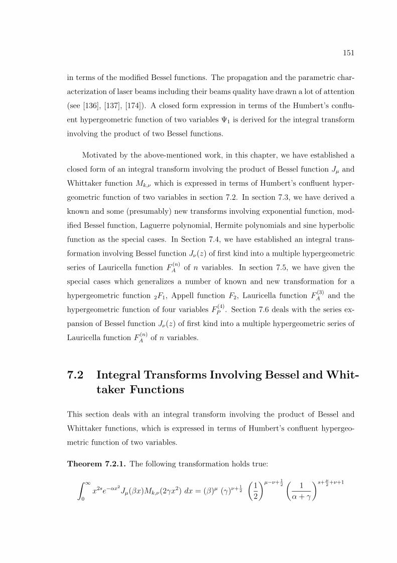
151

in terms of the modified Bessel functions. The propagation and the parametric char-

acterization of laser beams including their beams quality have drawn a lot of attention

(see [136], [137], [174]). A closed form expression in terms of the Humbert’s conflu-

ent hypergeometric function of two variables Ψ1 is derived for the integral transform

involving the product of two Bessel functions.

Motivated by the above-mentioned work, in this chapter, we have established a

closed form of an integral transform involving the product of Bessel function Jµ and

Whittaker function Mk,ν which is expressed in terms of Humbert’s confluent hyper-

geometric function of two variables in section 7.2. In section 7.3, we have derived a

known and some (presumably) new transforms involving exponential function, mod-

ified Bessel function, Laguerre polynomial, Hermite polynomials and sine hyperbolic

function as the special cases. In Section 7.4, we have established an integral trans-

formation involving Bessel function Jν(z) of first kind into a multiple hypergeometric

series of Lauricella function F(n)A of n variables. In section 7.5, we have given the

special cases which generalizes a number of known and new transformation for a

hypergeometric function 2F1, Appell function F2, Lauricella function F(3)A and the

hypergeometric function of four variables F(4)P . Section 7.6 deals with the series ex-

pansion of Bessel function Jν(z) of first kind into a multiple hypergeometric series of

Lauricella function F(n)A of n variables.

7.2 Integral Transforms Involving Bessel and Whit-

taker Functions

This section deals with an integral transform involving the product of Bessel and

Whittaker functions, which is expressed in terms of Humbert’s confluent hypergeo-

metric function of two variables.

Theorem 7.2.1. The following transformation holds true:

∫ ∞0

x2se−αx2

Jµ(βx)Mk,ν(2γx2) dx = (β)µ (γ)ν+ 1

2

(1

2

)µ−ν+ 12(

1

α + γ

)s+µ2

+ν+1

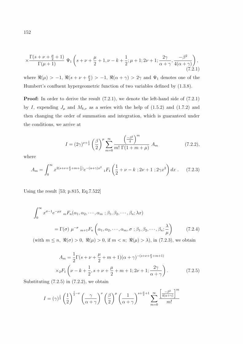
152

×Γ(s+ ν + µ

2+ 1)

Γ(µ+ 1)Ψ1

(s+ ν +

µ

2+ 1, ν − k +

1

2;µ+ 1; 2ν + 1;

2γ

α + γ,−β2

4(α + γ)

),

(7.2.1)

where <(µ) > −1, <(s + ν + µ2) > −1, <(α + γ) > 2γ and Ψ1 denotes one of the

Humbert’s confluent hypergeometric function of two variables defined by (1.3.8).

Proof: In order to derive the result (7.2.1), we denote the left-hand side of (7.2.1)

by I, expending Jµ and Mk,ν as a series with the help of (1.5.2) and (1.7.2) and

then changing the order of summation and integration, which is guaranteed under

the conditions, we arrive at

I = (2γ)ν+ 12

(β

2

)µ ∞∑m=0

(−β2

4

)mm! Γ(1 +m+ µ)

Am (7.2.2),

where

Am =

∫ ∞0

x2(s+ν+µ2

+m+ 12

)e−(α+γ)x21F1

(1

2+ ν − k ; 2ν + 1 ; 2γx2

)dx . (7.2.3)

Using the result [53; p.815, Eq.7.522]

∫ ∞0

xσ−1e−µx mFn(α1, α2, · · · , αm ; β1, β2, · · · , βn;λx)

= Γ(σ) µ−σ m+1Fn

(α1, α2, · · · , αm, σ ; β1, β2, · · · , βn;

λ

µ

)(7.2.4)

(with m ≤ n, <(σ) > 0, <(µ) > 0, if m < n; <(µ) > λ), in (7.2.3), we obtain

Am =1

2Γ(s+ ν +

µ

2+m+ 1)(α + γ)−(s+ν+µ

2+m+1)

×2F1

(ν − k +

1

2, s+ ν +

µ

2+m+ 1; 2ν + 1;

2γ

α + γ

). (7.2.5)

Substituting (7.2.5) in (7.2.2), we obtain

I = (γ)12

(1

2

) 12−ν (

γ

α + γ

)ν (β

2

)µ(1

α + γ

)s+µ2

+1 ∞∑m=0

[−β2

4(α+γ)

]mm!

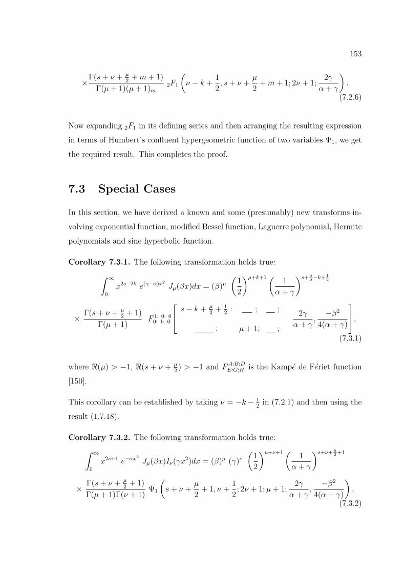
153

×Γ(s+ ν + µ

2+m+ 1)

Γ(µ+ 1)(µ+ 1)m2F1

(ν − k +

1

2, s+ ν +

µ

2+m+ 1; 2ν + 1;

2γ

α + γ

).

(7.2.6)

Now expanding 2F1 in its defining series and then arranging the resulting expression

in terms of Humbert’s confluent hypergeometric function of two variables Ψ1, we get

the required result. This completes the proof.

7.3 Special Cases

In this section, we have derived a known and some (presumably) new transforms in-

volving exponential function, modified Bessel function, Laguerre polynomial, Hermite

polynomials and sine hyperbolic function.

Corollary 7.3.1. The following transformation holds true:∫ ∞0

x2s−2k e(γ−α)x2 Jµ(βx)dx = (β)µ(

1

2

)µ+k+1(1

α + γ

)s+µ2−k+ 1

2

×Γ(s+ ν + µ

2+ 1)

Γ(µ+ 1)F 1: 0: 0

0: 1; 0

s− k + µ2

+ 12

: ; ;

: µ+ 1; ;

2γ

α + γ,−β2

4(α + γ)

,(7.3.1)

where <(µ) > −1, <(s + ν + µ2) > −1 and FA:B;D

E:G;H is the Kampe de Feriet function

[150].

This corollary can be established by taking ν = −k− 12

in (7.2.1) and then using the

result (1.7.18).

Corollary 7.3.2. The following transformation holds true:∫ ∞0

x2s+1 e−αx2

Jµ(βx)Iν(γx2)dx = (β)µ (γ)ν

(1

2

)µ+ν+1(1

α + γ

)s+ν+µ2

+1

×Γ(s+ ν + µ

2+ 1)

Γ(µ+ 1)Γ(ν + 1)Ψ1

(s+ ν +

µ

2+ 1, ν +

1

2; 2ν + 1;µ+ 1;

2γ

α + γ,−β2

4(α + γ)

),

(7.3.2)

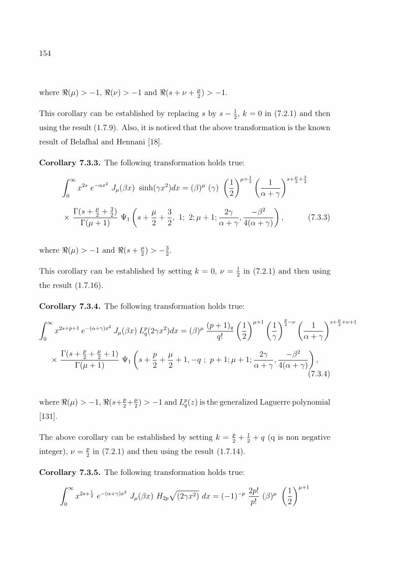
154

where <(µ) > −1, <(ν) > −1 and <(s+ ν + µ2) > −1.

This corollary can be established by replacing s by s − 12, k = 0 in (7.2.1) and then

using the result (1.7.9). Also, it is noticed that the above transformation is the known

result of Belafhal and Hennani [18].

Corollary 7.3.3. The following transformation holds true:∫ ∞0

x2s e−αx2

Jµ(βx) sinh(γx2)dx = (β)µ (γ)

(1

2

)µ+ 12(

1

α + γ

)s+µ2

+ 32

×Γ(s+ µ

2+ 3

2)

Γ(µ+ 1)Ψ1

(s+

µ

2+

3

2, 1; 2;µ+ 1;

2γ

α + γ,−β2

4(α + γ)

), (7.3.3)

where <(µ) > −1 and <(s+ µ2) > −3

2.

This corollary can be established by setting k = 0, ν = 12

in (7.2.1) and then using

the result (1.7.16).

Corollary 7.3.4. The following transformation holds true:∫ ∞0

x2s+p+1 e−(α+γ)x2 Jµ(βx) Lpq(2γx2)dx = (β)µ

(p+ 1)qq!

(1

2

)µ+1(1

γ

) p2−ν (

1

α + γ

)s+µ2

+ν+1

×Γ(s+ p

2+ µ

2+ 1)

Γ(µ+ 1)Ψ1

(s+

p

2+µ

2+ 1,−q ; p+ 1;µ+ 1;

2γ

α + γ,−β2

4(α + γ)

),

(7.3.4)

where <(µ) > −1, <(s+ p2+ µ

2) > −1 and Lpq(z) is the generalized Laguerre polynomial

[131].

The above corollary can be established by setting k = p2

+ 12

+ q (q is non negative

integer), ν = p2

in (7.2.1) and then using the result (1.7.14).

Corollary 7.3.5. The following transformation holds true:∫ ∞0

x2s+ 12 e−(α+γ)x2 Jµ(βx) H2p

√(2γx2) dx = (−1)−p

2p!

p!(β)µ

(1

2

)µ+1

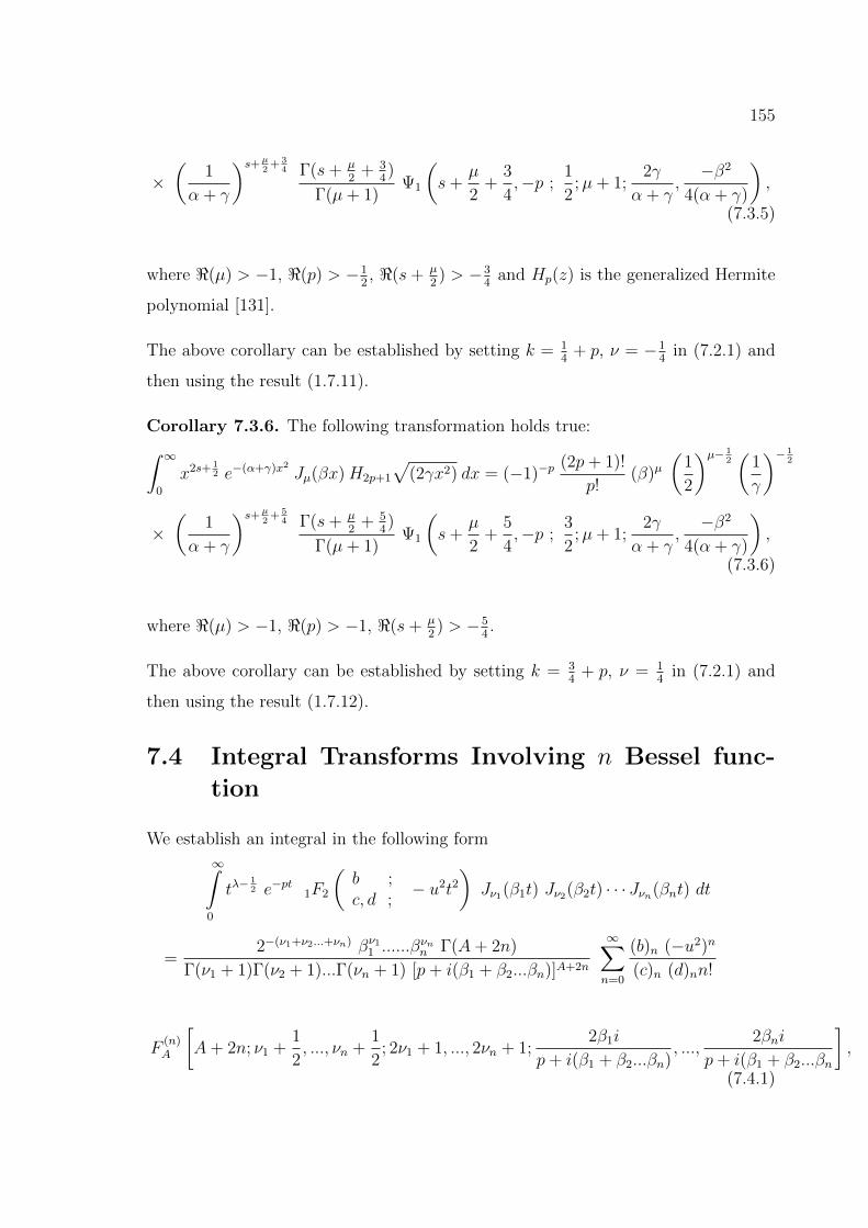
155

×(

1

α + γ

)s+µ2

+ 34 Γ(s+ µ

2+ 3

4)

Γ(µ+ 1)Ψ1

(s+

µ

2+

3

4,−p ;

1

2;µ+ 1;

2γ

α + γ,−β2

4(α + γ)

),

(7.3.5)

where <(µ) > −1, <(p) > −12, <(s+ µ

2) > −3

4and Hp(z) is the generalized Hermite

polynomial [131].

The above corollary can be established by setting k = 14

+ p, ν = −14

in (7.2.1) and

then using the result (1.7.11).

Corollary 7.3.6. The following transformation holds true:∫ ∞0

x2s+ 12 e−(α+γ)x2 Jµ(βx)H2p+1

√(2γx2) dx = (−1)−p

(2p+ 1)!

p!(β)µ

(1

2

)µ− 12(

1

γ

)− 12

×(

1

α + γ

)s+µ2

+ 54 Γ(s+ µ

2+ 5

4)

Γ(µ+ 1)Ψ1

(s+

µ

2+

5

4,−p ;

3

2;µ+ 1;

2γ

α + γ,−β2

4(α + γ)

),

(7.3.6)

where <(µ) > −1, <(p) > −1, <(s+ µ2) > −5

4.

The above corollary can be established by setting k = 34

+ p, ν = 14

in (7.2.1) and

then using the result (1.7.12).

7.4 Integral Transforms Involving n Bessel func-

tion

We establish an integral in the following form

∞∫0

tλ−12 e−pt 1F2

(b ;c, d ;

− u2t2)Jν1(β1t) Jν2(β2t) · · · Jνn(βnt) dt

=2−(ν1+ν2...+νn) βν11 ......β

νnn Γ(A+ 2n)

Γ(ν1 + 1)Γ(ν2 + 1)...Γ(νn + 1) [p+ i(β1 + β2...βn)]A+2n

∞∑n=0

(b)n (−u2)n

(c)n (d)nn!

F(n)A

[A+ 2n; ν1 +

1

2, ..., νn +

1

2; 2ν1 + 1, ..., 2νn + 1;

2β1i

p+ i(β1 + β2...βn), ...,

2βni

p+ i(β1 + β2...βn

],

(7.4.1)

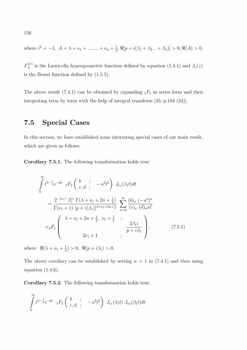
156

where i2 = −1, A = λ+ ν1 + ........+ νn + 12,<[p+ i(β1 + β2...+ βn)] > 0,<(A) > 0,

F(n)A is the Lauricella hypergeometric function defined by equation (1.4.1) and Jν(z)

is the Bessel function defined by (1.5.5).

The above result (7.4.1) can be obtained by expanding 1F2 in series form and then

integrating term by term with the help of integral transform [45; p.184 (24)].

7.5 Special Cases

In this section, we have established some interesting special cases of our main result,

which are given as follows:

Corollary 7.5.1. The following transformation holds true:

∞∫0

tλ−12 e−pt 1F2

(b ;c, d ;

− u2t2)Jν1(β1t)dt

=2−(ν1) βν11 Γ(λ+ ν1 + 2n+ 1

2)

Γ(ν1 + 1) [p+ i(β1)]λ+ν1+2n+ 12

∞∑n=0

(b)n (−u2)n

(c)n (d)nn!

×2F1

λ+ ν1 + 2n+ 1

2, ν1 + 1

2;

2β1i

p+ iβ1

2ν1 + 1 ;

, (7.5.1)

where <(λ+ ν1 + 12) > 0, <(p+ iβ1) > 0.

The above corollary can be established by setting n = 1 in (7.4.1) and then using

equation (1.4.6).

Corollary 7.5.2. The following transformation holds true:

∞∫0

tλ−12 e−pt 1F2

(b ;c, d ;

− u2t2)Jν1(β1t) Jν2(β2t)dt

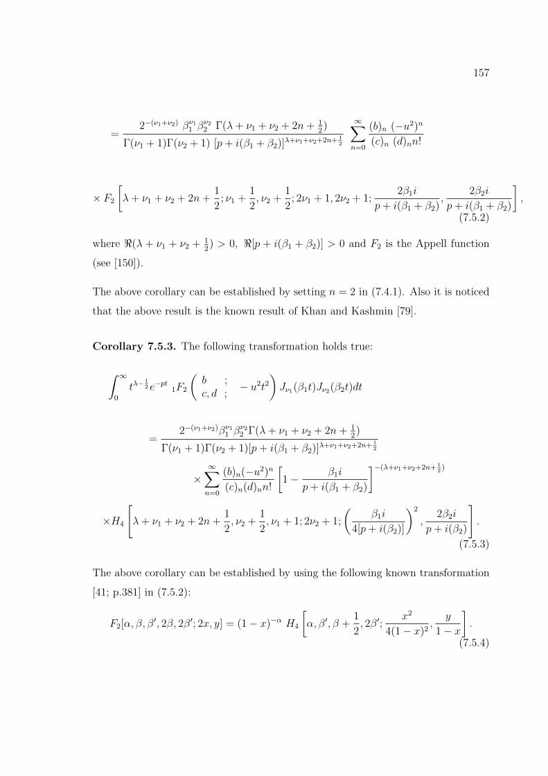
157

=2−(ν1+ν2) βν11 β

ν22 Γ(λ+ ν1 + ν2 + 2n+ 1

2)

Γ(ν1 + 1)Γ(ν2 + 1) [p+ i(β1 + β2)]λ+ν1+ν2+2n+ 12

∞∑n=0

(b)n (−u2)n

(c)n (d)nn!

× F2

[λ+ ν1 + ν2 + 2n+

1

2; ν1 +

1

2, ν2 +

1

2; 2ν1 + 1, 2ν2 + 1;

2β1i

p+ i(β1 + β2),

2β2i

p+ i(β1 + β2)

],

(7.5.2)

where <(λ + ν1 + ν2 + 12) > 0, <[p + i(β1 + β2)] > 0 and F2 is the Appell function

(see [150]).

The above corollary can be established by setting n = 2 in (7.4.1). Also it is noticed

that the above result is the known result of Khan and Kashmin [79].

Corollary 7.5.3. The following transformation holds true:

∫ ∞0

tλ−12 e−pt 1F2

(b ;c, d ;

− u2t2)Jν1(β1t)Jν2(β2t)dt

=2−(ν1+ν2)βν11 β

ν22 Γ(λ+ ν1 + ν2 + 2n+ 1

2)

Γ(ν1 + 1)Γ(ν2 + 1)[p+ i(β1 + β2)]λ+ν1+ν2+2n+ 12

×∞∑n=0

(b)n(−u2)n

(c)n(d)nn!

[1− β1i

p+ i(β1 + β2)

]−(λ+ν1+ν2+2n+ 12

)

×H4

[λ+ ν1 + ν2 + 2n+

1

2, ν2 +

1

2, ν1 + 1; 2ν2 + 1;

(β1i

4[p+ i(β2)]

)2

,2β2i

p+ i(β2)

].

(7.5.3)

The above corollary can be established by using the following known transformation

[41; p.381] in (7.5.2):

F2[α, β, β′, 2β, 2β′; 2x, y] = (1− x)−α H4

[α, β′, β +

1

2, 2β′;

x2

4(1− x)2,

y

1− x

].

(7.5.4)

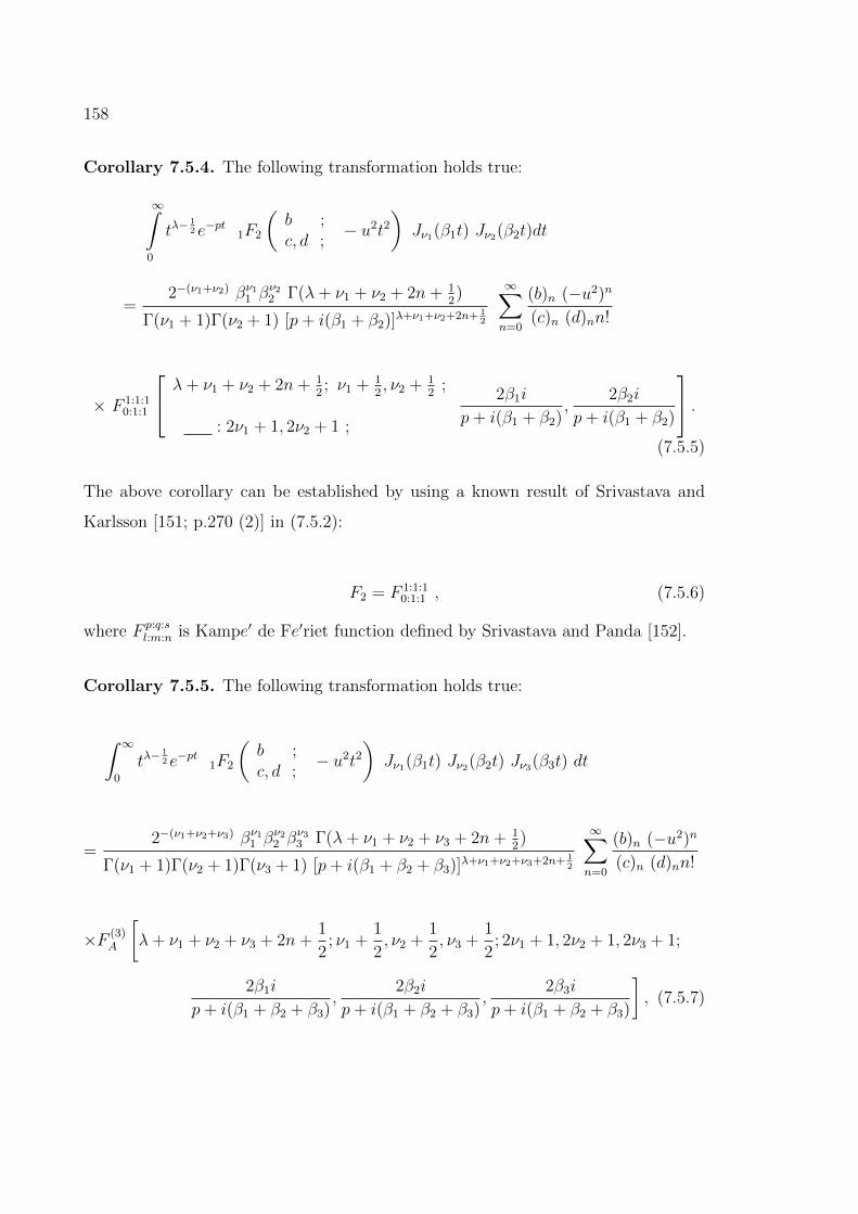
158

Corollary 7.5.4. The following transformation holds true:

∞∫0

tλ−12 e−pt 1F2

(b ;c, d ;

− u2t2)Jν1(β1t) Jν2(β2t)dt

=2−(ν1+ν2) βν11 β

ν22 Γ(λ+ ν1 + ν2 + 2n+ 1

2)

Γ(ν1 + 1)Γ(ν2 + 1) [p+ i(β1 + β2)]λ+ν1+ν2+2n+ 12

∞∑n=0

(b)n (−u2)n

(c)n (d)nn!

× F 1:1:10:1:1

λ+ ν1 + ν2 + 2n+ 12; ν1 + 1

2, ν2 + 1

2;

: 2ν1 + 1, 2ν2 + 1 ;

2β1i

p+ i(β1 + β2),

2β2i

p+ i(β1 + β2)

.(7.5.5)

The above corollary can be established by using a known result of Srivastava and

Karlsson [151; p.270 (2)] in (7.5.2):

F2 = F 1:1:10:1:1 , (7.5.6)

where F p:q:sl:m:n is Kampe′ de Fe′riet function defined by Srivastava and Panda [152].

Corollary 7.5.5. The following transformation holds true:

∫ ∞0

tλ−12 e−pt 1F2

(b ;c, d ;

− u2t2)Jν1(β1t) Jν2(β2t) Jν3(β3t) dt

=2−(ν1+ν2+ν3) βν11 β

ν22 β

ν33 Γ(λ+ ν1 + ν2 + ν3 + 2n+ 1

2)

Γ(ν1 + 1)Γ(ν2 + 1)Γ(ν3 + 1) [p+ i(β1 + β2 + β3)]λ+ν1+ν2+ν3+2n+ 12

∞∑n=0

(b)n (−u2)n

(c)n (d)nn!

×F (3)A

[λ+ ν1 + ν2 + ν3 + 2n+

1

2; ν1 +

1

2, ν2 +

1

2, ν3 +

1

2; 2ν1 + 1, 2ν2 + 1, 2ν3 + 1;

2β1i

p+ i(β1 + β2 + β3),

2β2i

p+ i(β1 + β2 + β3),

2β3i

p+ i(β1 + β2 + β3)

], (7.5.7)

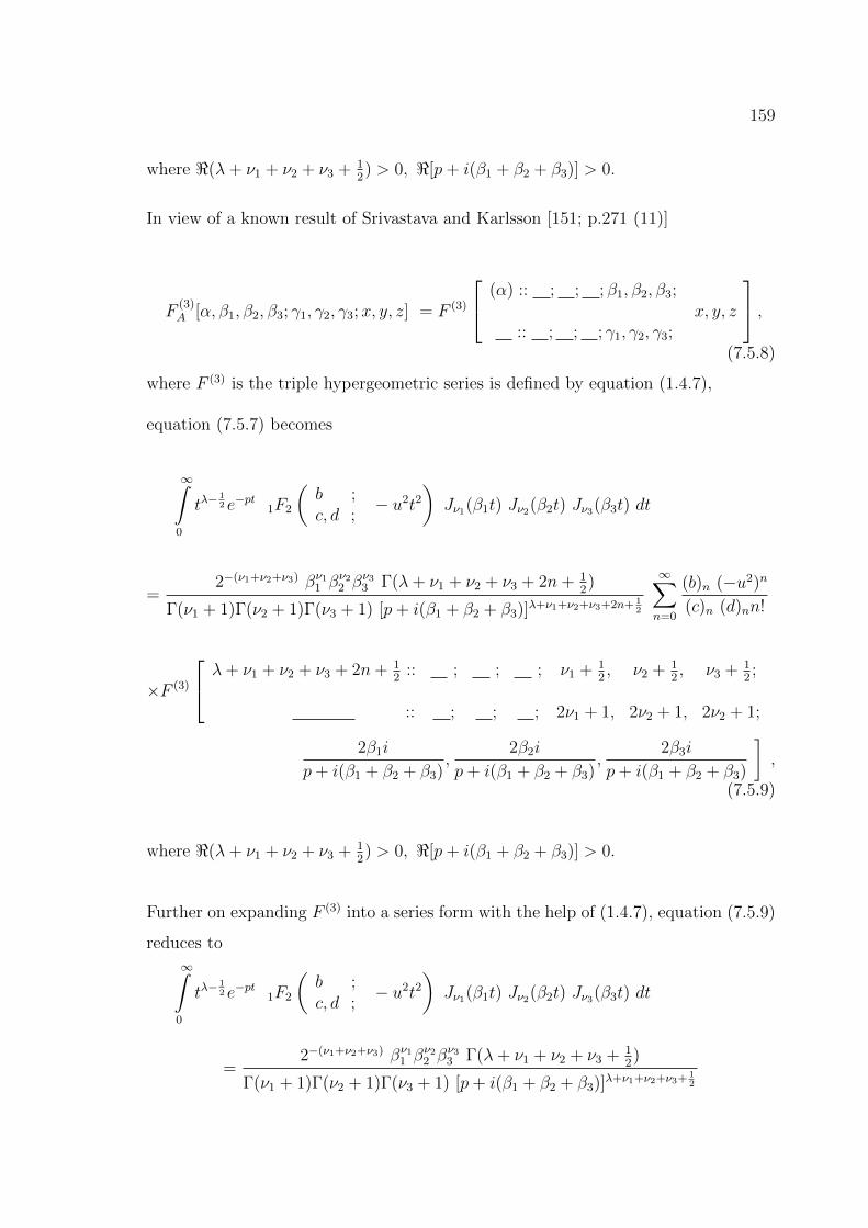
159

where <(λ+ ν1 + ν2 + ν3 + 12) > 0, <[p+ i(β1 + β2 + β3)] > 0.

In view of a known result of Srivastava and Karlsson [151; p.271 (11)]

F(3)A [α, β1, β2, β3; γ1, γ2, γ3;x, y, z] = F (3)

(α) :: ; ; ; β1, β2, β3;

:: ; ; ; γ1, γ2, γ3;x, y, z

,(7.5.8)

where F (3) is the triple hypergeometric series is defined by equation (1.4.7),

equation (7.5.7) becomes

∞∫0

tλ−12 e−pt 1F2

(b ;c, d ;

− u2t2)Jν1(β1t) Jν2(β2t) Jν3(β3t) dt

=2−(ν1+ν2+ν3) βν11 β

ν22 β

ν33 Γ(λ+ ν1 + ν2 + ν3 + 2n+ 1

2)

Γ(ν1 + 1)Γ(ν2 + 1)Γ(ν3 + 1) [p+ i(β1 + β2 + β3)]λ+ν1+ν2+ν3+2n+ 12

∞∑n=0

(b)n (−u2)n

(c)n (d)nn!

×F (3)

λ+ ν1 + ν2 + ν3 + 2n+ 12

:: ; ; ; ν1 + 12, ν2 + 1

2, ν3 + 1

2;

:: ; ; ; 2ν1 + 1, 2ν2 + 1, 2ν2 + 1;

2β1i

p+ i(β1 + β2 + β3),

2β2i

p+ i(β1 + β2 + β3),

2β3i

p+ i(β1 + β2 + β3)

],

(7.5.9)

where <(λ+ ν1 + ν2 + ν3 + 12) > 0, <[p+ i(β1 + β2 + β3)] > 0.

Further on expanding F (3) into a series form with the help of (1.4.7), equation (7.5.9)

reduces to

∞∫0

tλ−12 e−pt 1F2

(b ;c, d ;

− u2t2)Jν1(β1t) Jν2(β2t) Jν3(β3t) dt

=2−(ν1+ν2+ν3) βν11 β

ν22 β

ν33 Γ(λ+ ν1 + ν2 + ν3 + 1

2)

Γ(ν1 + 1)Γ(ν2 + 1)Γ(ν3 + 1) [p+ i(β1 + β2 + β3)]λ+ν1+ν2+ν3+ 12

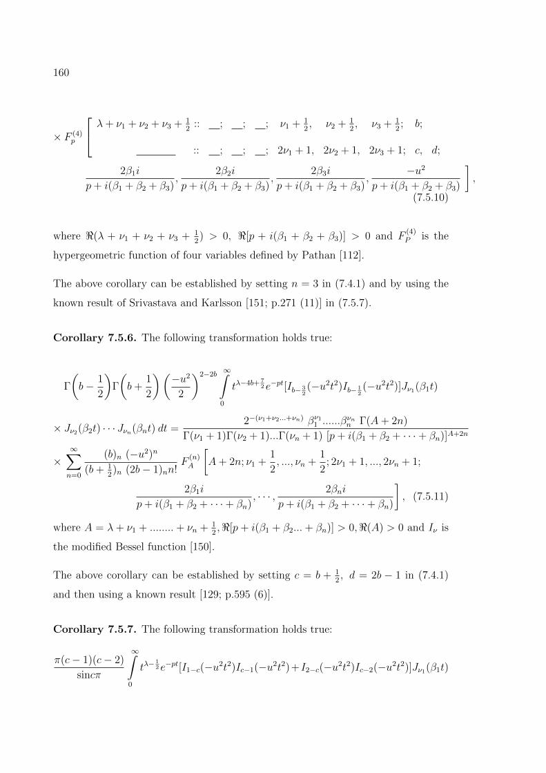
160

× F (4)p

λ+ ν1 + ν2 + ν3 + 12

:: ; ; ; ν1 + 12, ν2 + 1

2, ν3 + 1

2; b;

:: ; ; ; 2ν1 + 1, 2ν2 + 1, 2ν3 + 1; c, d;

2β1i

p+ i(β1 + β2 + β3),

2β2i

p+ i(β1 + β2 + β3),

2β3i

p+ i(β1 + β2 + β3),

−u2

p+ i(β1 + β2 + β3)

],

(7.5.10)

where <(λ + ν1 + ν2 + ν3 + 12) > 0, <[p + i(β1 + β2 + β3)] > 0 and F

(4)P is the

hypergeometric function of four variables defined by Pathan [112].

The above corollary can be established by setting n = 3 in (7.4.1) and by using the

known result of Srivastava and Karlsson [151; p.271 (11)] in (7.5.7).

Corollary 7.5.6. The following transformation holds true:

Γ

(b− 1

2

)Γ

(b+

1

2

)(−u2

2

)2−2b∞∫

0

tλ−4b+ 72 e−pt[Ib− 3

2(−u2t2)Ib− 1

2(−u2t2)]Jν1(β1t)

× Jν2(β2t) · · · Jνn(βnt) dt =2−(ν1+ν2...+νn) βν11 ......β

νnn Γ(A+ 2n)

Γ(ν1 + 1)Γ(ν2 + 1)...Γ(νn + 1) [p+ i(β1 + β2 + · · ·+ βn)]A+2n

×∞∑n=0

(b)n (−u2)n

(b+ 12)n (2b− 1)nn!

F(n)A

[A+ 2n; ν1 +

1

2, ..., νn +

1

2; 2ν1 + 1, ..., 2νn + 1;

2β1i

p+ i(β1 + β2 + · · ·+ βn), · · · , 2βni

p+ i(β1 + β2 + · · ·+ βn)

], (7.5.11)

where A = λ + ν1 + ........ + νn + 12,<[p + i(β1 + β2... + βn)] > 0,<(A) > 0 and Iν is

the modified Bessel function [150].

The above corollary can be established by setting c = b + 12, d = 2b − 1 in (7.4.1)

and then using a known result [129; p.595 (6)].

Corollary 7.5.7. The following transformation holds true:

π(c− 1)(c− 2)

sincπ

∞∫0

tλ−12 e−pt[I1−c(−u2t2)Ic−1(−u2t2)+I2−c(−u2t2)Ic−2(−u2t2)]Jν1(β1t)

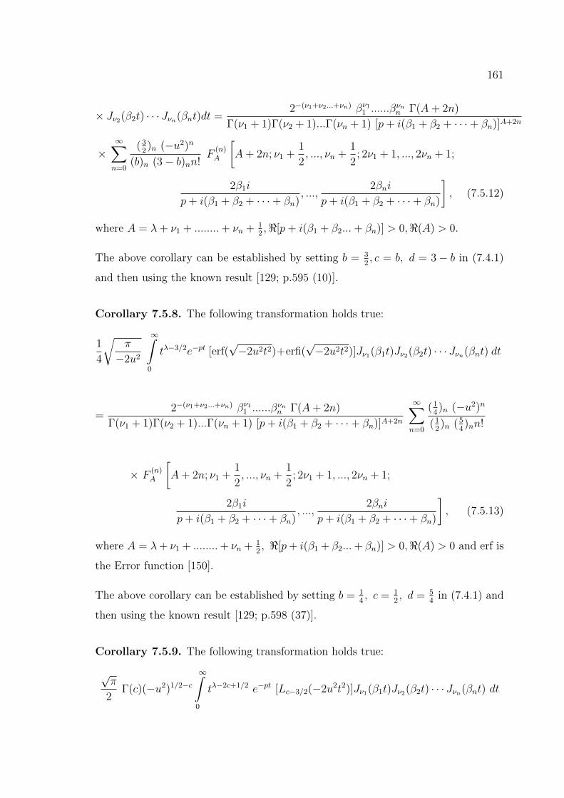
161

× Jν2(β2t) · · · Jνn(βnt)dt =2−(ν1+ν2...+νn) βν11 ......β

νnn Γ(A+ 2n)

Γ(ν1 + 1)Γ(ν2 + 1)...Γ(νn + 1) [p+ i(β1 + β2 + · · ·+ βn)]A+2n

×∞∑n=0

(32)n (−u2)n

(b)n (3− b)nn!F

(n)A

[A+ 2n; ν1 +

1

2, ..., νn +

1

2; 2ν1 + 1, ..., 2νn + 1;

2β1i

p+ i(β1 + β2 + · · ·+ βn), ...,

2βni

p+ i(β1 + β2 + · · ·+ βn)

], (7.5.12)

where A = λ+ ν1 + ........+ νn + 12,<[p+ i(β1 + β2...+ βn)] > 0,<(A) > 0.

The above corollary can be established by setting b = 32, c = b, d = 3− b in (7.4.1)

and then using the known result [129; p.595 (10)].

Corollary 7.5.8. The following transformation holds true:

1

4

√π

−2u2

∞∫0

tλ−3/2e−pt [erf(√−2u2t2)+erfi(

√−2u2t2)]Jν1(β1t)Jν2(β2t) · · · Jνn(βnt) dt

=2−(ν1+ν2...+νn) βν11 ......β

νnn Γ(A+ 2n)

Γ(ν1 + 1)Γ(ν2 + 1)...Γ(νn + 1) [p+ i(β1 + β2 + · · ·+ βn)]A+2n

∞∑n=0

(14)n (−u2)n

(12)n (5

4)nn!

× F(n)A

[A+ 2n; ν1 +

1

2, ..., νn +

1

2; 2ν1 + 1, ..., 2νn + 1;

2β1i

p+ i(β1 + β2 + · · ·+ βn), ...,

2βni

p+ i(β1 + β2 + · · ·+ βn)

], (7.5.13)

where A = λ+ ν1 + ........+ νn + 12, <[p+ i(β1 + β2...+ βn)] > 0,<(A) > 0 and erf is

the Error function [150].

The above corollary can be established by setting b = 14, c = 1

2, d = 5

4in (7.4.1) and

then using the known result [129; p.598 (37)].

Corollary 7.5.9. The following transformation holds true:

√π

2Γ(c)(−u2)1/2−c

∞∫0

tλ−2c+1/2 e−pt [Lc−3/2(−2u2t2)]Jν1(β1t)Jν2(β2t) · · · Jνn(βnt) dt

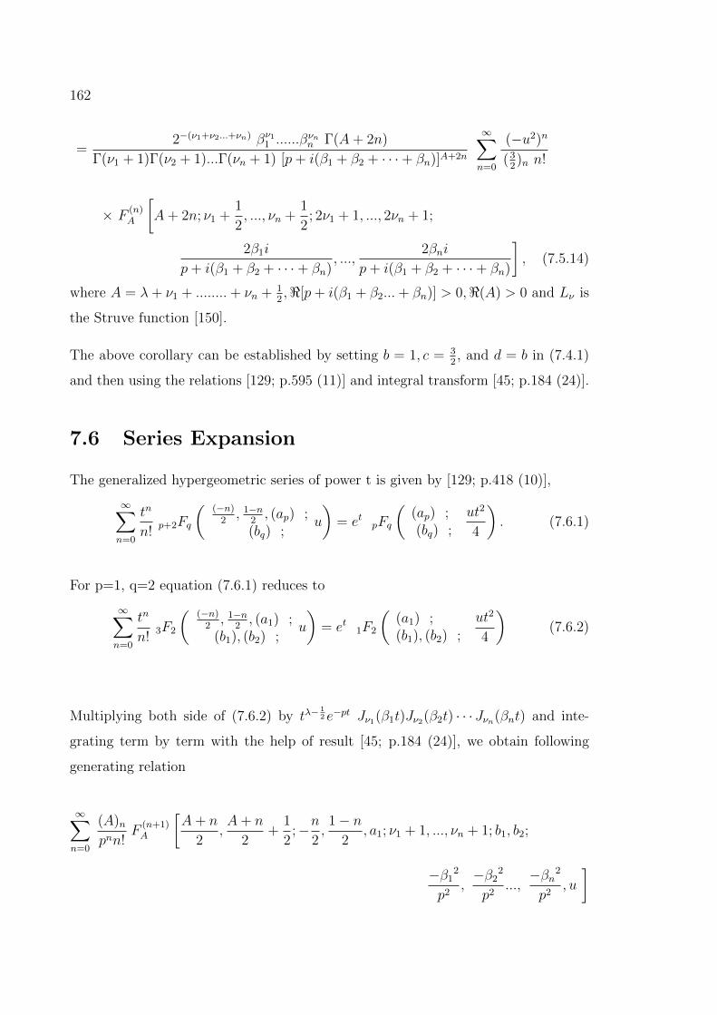
162

=2−(ν1+ν2...+νn) βν11 ......β

νnn Γ(A+ 2n)

Γ(ν1 + 1)Γ(ν2 + 1)...Γ(νn + 1) [p+ i(β1 + β2 + · · ·+ βn)]A+2n

∞∑n=0

(−u2)n

(32)n n!

× F(n)A

[A+ 2n; ν1 +

1

2, ..., νn +

1

2; 2ν1 + 1, ..., 2νn + 1;

2β1i

p+ i(β1 + β2 + · · ·+ βn), ...,

2βni

p+ i(β1 + β2 + · · ·+ βn)

], (7.5.14)

where A = λ+ ν1 + ........+ νn + 12,<[p+ i(β1 + β2...+ βn)] > 0,<(A) > 0 and Lν is

the Struve function [150].

The above corollary can be established by setting b = 1, c = 32, and d = b in (7.4.1)

and then using the relations [129; p.595 (11)] and integral transform [45; p.184 (24)].

7.6 Series Expansion

The generalized hypergeometric series of power t is given by [129; p.418 (10)],

∞∑n=0

tn

n!p+2Fq

((−n)

2, 1−n

2, (ap) ;

(bq) ;u

)= et pFq

((ap) ;(bq) ;

ut2

4

). (7.6.1)

For p=1, q=2 equation (7.6.1) reduces to

∞∑n=0

tn

n!3F2

((−n)

2, 1−n

2, (a1) ;

(b1), (b2) ;u

)= et 1F2

((a1) ;(b1), (b2) ;

ut2

4

)(7.6.2)

Multiplying both side of (7.6.2) by tλ−12 e−pt Jν1(β1t)Jν2(β2t) · · · Jνn(βnt) and inte-

grating term by term with the help of result [45; p.184 (24)], we obtain following

generating relation

∞∑n=0

(A)npnn!

F(n+1)A

[A+ n

2,A+ n

2+

1

2;−n

2,1− n

2, a1; ν1 + 1, ..., νn + 1; b1, b2;

−β12

p2,−β2

2

p2...,−βn2

p2, u

]

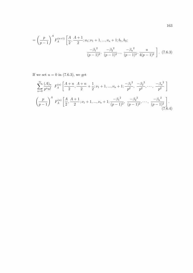
163

=

(p

p− 1

)AF

(n+1)A

[A

2,A+ 1

2; a1; ν1 + 1, ..., νn + 1; b1, b2;

−β12

(p− 1)2,−β2

2

(p− 1)2...,

−βn2

(p− 1)2,

u

4(p− 1)2

]. (7.6.3)

If we set u = 0 in (7.6.3), we get

∞∑n=0

(A)npnn!

F(n)A

[A+ n

2,A+ n

2+

1

2; ν1 + 1, ..., νn + 1;

−β12

p2,−β2

2

p2, · · · , −βn

2

p2

](

p

p− 1

)AF

(n)A

[A

2,A+ 1

2; ν1 + 1, ..., νn + 1;

−β12

(p− 1)2,−β2

2

(p− 1)2, · · · , −βn2

(p− 1)2

].

(7.6.4)

Chapter 8

Study of Unified IntegralsAssociated with WhittakerFunction

8.1 Introduction

Many important functions in applied sciences are defined via improper integrals or

series (or infinite products). The general name of these important functions are called

special functions. Bessel function are important special functions and their closely

related ones are widely used in physics and engineering; therefore, they are of interest

to physicists and engineers as well as mathematicians. In recent years, numerous in-

tegral formulas involving a variety of special functions have been developed by many

authors (see, [4], [15], [22], [31], [51] and [75]). Recently Khan and Ghayasuddin

[77] established some interesting unified integrals involving the Whittaker function of

first kind Mρ,σ(z). Afterwards Khan and Ghayasuddin [78] defined some another new

integral formulas involving generalized Bessel function wbν,c(z), in terms of Wright hy-

pergeometric function.

The main object of the present chapter is to obtain some unified integral formulas

involving Whittaker functions of the first kind into a series of Kampe de Feriet

function. Some integrals which are used to obtain our main results are included

in section 8.2. Section 8.3 gives interesting Lavoie and Trottier integral formulas

involving Whittaker function of first kind, some special cases of these results are

164

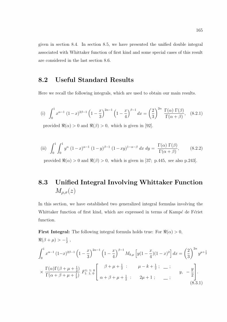
165

given in section 8.4. In section 8.5, we have presented the unified double integral

associated with Whittaker function of first kind and some special cases of this result

are considered in the last section 8.6.

8.2 Useful Standard Results

Here we recall the following integrals, which are used to obtain our main results.

(i)

∫ 1

0

xα−1 (1−x)2β−1(

1− x

3

)2α−1 (1− x

4

)β−1

dx =

(2

3

)2αΓ(α) Γ(β)

Γ(α + β), (8.2.1)

provided <(α) > 0 and <(β) > 0, which is given in [92].

(ii)

∫ 1

0

∫ 1

0

yα (1−x)α−1 (1− y)β−1 (1−xy)1−α−β dx dy =Γ(α) Γ(β)

Γ(α + β), (8.2.2)

provided <(α) > 0 and <(β) > 0, which is given in [37; p.445, see also p.243].

8.3 Unified Integral Involving Whittaker Function

Mρ,σ(z)

In this section, we have established two generalized integral formulas involving the

Whittaker function of first kind, which are expressed in terms of Kampe de Feriet

function.

First Integral: The following integral formula holds true: For <(α) > 0,

<(β + µ) > −12

,∫ 1

0

xα−1 (1−x)2β−1(

1− x

3

)2α−1 (1− x

4

)β−1

Mk,µ

[y(1− x

4)(1− x)2

]dx =

(2

3

)2α

yµ+ 12

×Γ(α)Γ(β + µ+ 1

2)

Γ(α + β + µ+ 12)F 1: 1: 0

1: 1; 0

β + µ+ 12

: µ− k + 12

; ;

α + β + µ+ 12

: 2µ+ 1 ; ;y, − y

2

.(8.3.1)

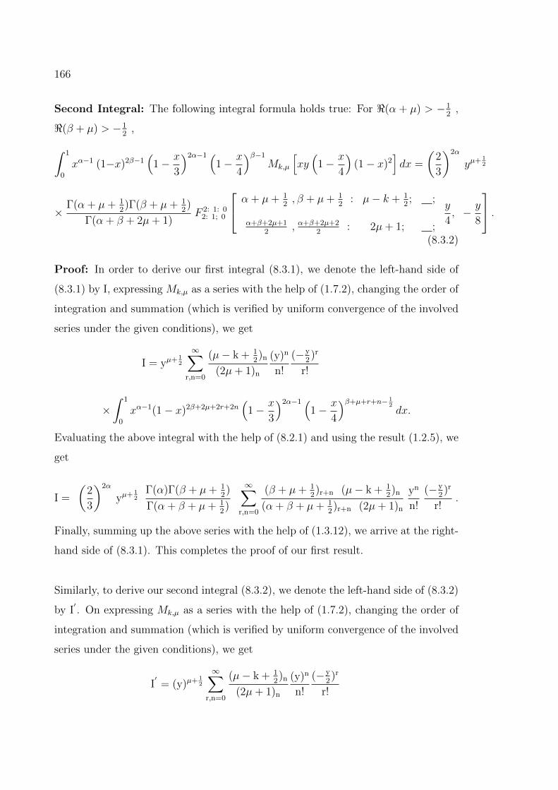
166

Second Integral: The following integral formula holds true: For <(α + µ) > −12,

<(β + µ) > −12

,∫ 1

0

xα−1 (1−x)2β−1(

1− x

3

)2α−1 (1− x

4

)β−1

Mk,µ

[xy(

1− x

4

)(1− x)2

]dx =

(2

3

)2α

yµ+ 12

×Γ(α + µ+ 1

2)Γ(β + µ+ 1

2)

Γ(α + β + 2µ+ 1)F 2: 1: 0

2: 1; 0

α + µ+ 12, β + µ+ 1

2: µ− k + 1

2; ;

α+β+2µ+12

, α+β+2µ+22

: 2µ+ 1; ;

y

4, − y

8

.(8.3.2)

Proof: In order to derive our first integral (8.3.1), we denote the left-hand side of

(8.3.1) by I, expressing Mk,µ as a series with the help of (1.7.2), changing the order of

integration and summation (which is verified by uniform convergence of the involved

series under the given conditions), we get

I = yµ+ 12

∞∑r,n=0

(µ− k + 12)n

(2µ+ 1)n

(y)n

n!

(−y2)r

r!

×∫ 1

0

xα−1(1− x)2β+2µ+2r+2n(

1− x

3

)2α−1 (1− x

4

)β+µ+r+n− 12dx.

Evaluating the above integral with the help of (8.2.1) and using the result (1.2.5), we

get

I =

(2

3

)2α

yµ+ 12

Γ(α)Γ(β + µ+ 12)

Γ(α + β + µ+ 12)

∞∑r,n=0

(β + µ+ 12)r+n (µ− k + 1

2)n

(α + β + µ+ 12)r+n (2µ+ 1)n

yn

n!

(−y2)r

r!.

Finally, summing up the above series with the help of (1.3.12), we arrive at the right-

hand side of (8.3.1). This completes the proof of our first result.

Similarly, to derive our second integral (8.3.2), we denote the left-hand side of (8.3.2)

by I′. On expressing Mk,µ as a series with the help of (1.7.2), changing the order of

integration and summation (which is verified by uniform convergence of the involved

series under the given conditions), we get

I′= (y)µ+ 1

2

∞∑r,n=0

(µ− k + 12)n

(2µ+ 1)n

(y)n

n!

(−y2)r

r!

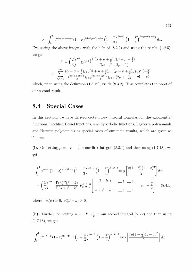
167

×∫ 1

0

xα+µ+r+n+ 12 (1− x)2β+2µ+2r+2n

(1− x

3

)2α−1 (1− x

4

)β+µ+r+n− 12dx.

Evaluating the above integral with the help of (8.2.2) and using the results (1.2.5),

we get

I′=

(2

3

)2α

(y)µ+ 12

Γ(α + µ+ 12)Γ(β + µ+ 1

2)

Γ(α + β + 2µ+ 1)

×∞∑

r,n=0

(α + µ+ 12)r+n(β + µ+ 1

2)r+n(µ− k + 1

2)n

(α+β+2µ+12

)r+n(α+β+2µ+22

)r+n (2µ+ 1)n

(y)n

n!

(−y2)r

r!.

which, upon using the definition (1.3.12), yields (8.3.2). This completes the proof of

our second result.

8.4 Special Cases

In this section, we have derived certain new integral formulas for the exponential

functions, modified Bessel functions, sine hyperbolic functions, Laguerre polynomials

and Hermite polynomials as special cases of our main results, which are given as

follows:

(i). On setting µ = −k − 12

in our first integral (8.3.1) and then using (1.7.18), we

get

∫ 1

0

xα−1 (1− x)2β−2k−1(

1− x

3

)2α−1 (1− x

4

)β−k−1

exp

[y(1− x

4)(1− x)2

2

]dx

=

(2

3

)2αΓ(α)Γ(β − k)

Γ(α + β − k)F 1: 0: 0

1: 0; 0

β − k : ; ;

α + β − k : ; ;y, − y

2

, (8.4.1)

where <(α) > 0, <(β − k) > 0.

(ii). Further, on setting µ = −k − 12

in our second integral (8.3.2) and then using

(1.7.18), we get

∫ 1

0

xα−k−1 (1−x)2β−2k−1(

1− x

3

)2α−1 (1− x

4

)β−k−1

exp

[xy(1− x

4)(1− x)2

2

]dx

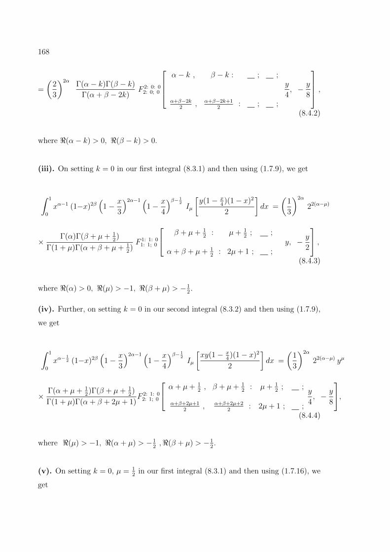
168

=

(2

3

)2αΓ(α− k)Γ(β − k)

Γ(α + β − 2k)F 2: 0: 0

2: 0; 0

α− k , β − k : ; ;

α+β−2k2

, α+β−2k+12

: ; ;

y

4, − y

8

,(8.4.2)

where <(α− k) > 0, <(β − k) > 0.

(iii). On setting k = 0 in our first integral (8.3.1) and then using (1.7.9), we get

∫ 1

0

xα−1 (1−x)2β(

1− x

3

)2α−1 (1− x

4

)β− 12Iµ

[y(1− x

4)(1− x)2

2

]dx =

(1

3

)2α

22(α−µ)

×Γ(α)Γ(β + µ+ 1

2)

Γ(1 + µ)Γ(α + β + µ+ 12)F 1: 1: 0

1: 1; 0

β + µ+ 12

: µ+ 12

; ;

α + β + µ+ 12

: 2µ+ 1 ; ;y, − y

2

,(8.4.3)

where <(α) > 0, <(µ) > −1, <(β + µ) > −12.

(iv). Further, on setting k = 0 in our second integral (8.3.2) and then using (1.7.9),

we get

∫ 1

0

xα−12 (1−x)2β

(1− x

3

)2α−1 (1− x

4

)β− 12Iµ

[xy(1− x

4)(1− x)2

2

]dx =

(1

3

)2α

22(α−µ) yµ

×Γ(α + µ+ 1

2)Γ(β + µ+ 1

2)

Γ(1 + µ)Γ(α + β + 2µ+ 1)F 2: 1: 0

2: 1; 0

α + µ+ 12, β + µ+ 1

2: µ+ 1

2; ;

α+β+2µ+12

, α+β+2µ+22

: 2µ+ 1 ; ;

y

4, − y

8

,(8.4.4)

where <(µ) > −1, <(α + µ) > −12,<(β + µ) > −1

2.

(v). On setting k = 0, µ = 12

in our first integral (8.3.1) and then using (1.7.16), we

get

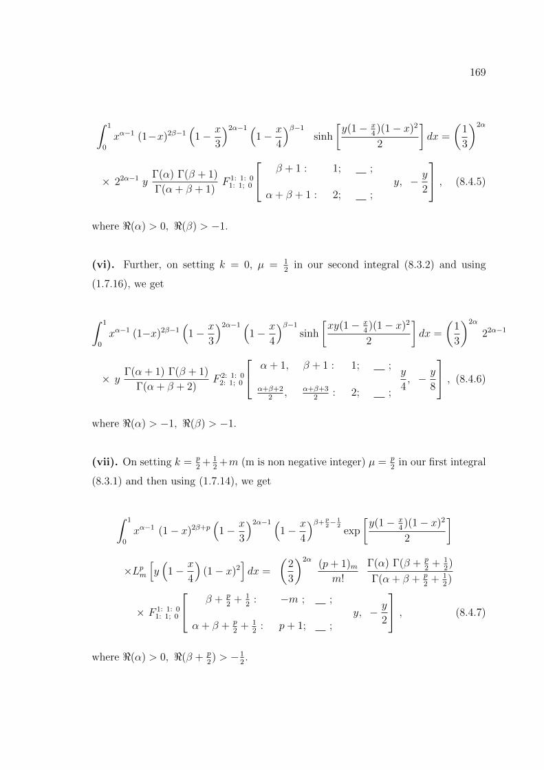
169

∫ 1

0

xα−1 (1−x)2β−1(

1− x

3

)2α−1 (1− x

4

)β−1

sinh

[y(1− x

4)(1− x)2

2

]dx =

(1

3

)2α

× 22α−1 yΓ(α) Γ(β + 1)

Γ(α + β + 1)F 1: 1: 0

1: 1; 0

β + 1 : 1; ;

α + β + 1 : 2; ;y, − y

2

, (8.4.5)

where <(α) > 0, <(β) > −1.

(vi). Further, on setting k = 0, µ = 12

in our second integral (8.3.2) and using

(1.7.16), we get

∫ 1

0

xα−1 (1−x)2β−1(

1− x

3

)2α−1 (1− x

4

)β−1

sinh

[xy(1− x

4)(1− x)2

2

]dx =

(1

3

)2α

22α−1

× yΓ(α + 1) Γ(β + 1)

Γ(α + β + 2)F 2: 1: 0

2: 1; 0

α + 1, β + 1 : 1; ;

α+β+22

, α+β+32

: 2; ;

y

4, − y

8

, (8.4.6)

where <(α) > −1, <(β) > −1.

(vii). On setting k = p2

+ 12

+m (m is non negative integer) µ = p2

in our first integral

(8.3.1) and then using (1.7.14), we get

∫ 1

0

xα−1 (1− x)2β+p(

1− x

3

)2α−1 (1− x

4

)β+ p2− 1

2exp

[y(1− x

4)(1− x)2

2

]

×Lpm[y(

1− x

4

)(1− x)2

]dx =

(2

3

)2α(p+ 1)mm!

Γ(α) Γ(β + p2

+ 12)

Γ(α + β + p2

+ 12)

× F 1: 1: 01: 1; 0

β + p2

+ 12

: −m ; ;

α + β + p2

+ 12

: p+ 1; ;y, − y

2

, (8.4.7)

where <(α) > 0, <(β + p2) > −1

2.

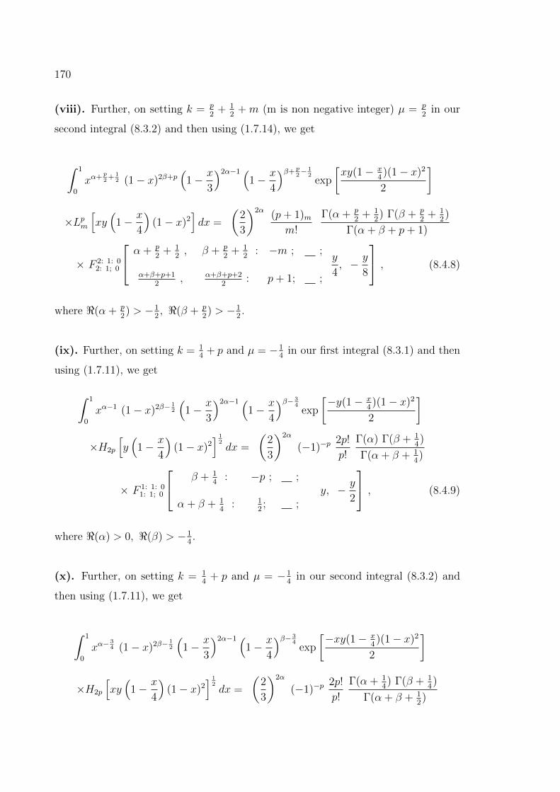
170

(viii). Further, on setting k = p2

+ 12

+ m (m is non negative integer) µ = p2

in our

second integral (8.3.2) and then using (1.7.14), we get

∫ 1

0

xα+ p2

+ 12 (1− x)2β+p

(1− x

3

)2α−1 (1− x

4

)β+ p2− 1

2exp

[xy(1− x

4)(1− x)2

2

]

×Lpm[xy(

1− x

4

)(1− x)2

]dx =

(2

3

)2α(p+ 1)mm!

Γ(α + p2

+ 12) Γ(β + p

2+ 1

2)

Γ(α + β + p+ 1)

× F 2: 1: 02: 1; 0

α + p2

+ 12, β + p

2+ 1

2: −m ; ;

α+β+p+12

, α+β+p+22

: p+ 1; ;

y

4, − y

8

, (8.4.8)

where <(α + p2) > −1

2, <(β + p

2) > −1

2.

(ix). Further, on setting k = 14

+ p and µ = −14

in our first integral (8.3.1) and then

using (1.7.11), we get

∫ 1

0

xα−1 (1− x)2β− 12

(1− x

3

)2α−1 (1− x

4

)β− 34

exp

[−y(1− x4)(1− x)2

2

]

×H2p

[y(

1− x

4

)(1− x)2

] 12dx =

(2

3

)2α

(−1)−p2p!

p!

Γ(α) Γ(β + 14)

Γ(α + β + 14)

× F 1: 1: 01: 1; 0

β + 14

: −p ; ;

α + β + 14

: 12; ;

y, − y

2

, (8.4.9)

where <(α) > 0, <(β) > −14.

(x). Further, on setting k = 14

+ p and µ = −14

in our second integral (8.3.2) and

then using (1.7.11), we get

∫ 1

0

xα−34 (1− x)2β− 1

2

(1− x

3

)2α−1 (1− x

4

)β− 34

exp

[−xy(1− x4)(1− x)2

2

]

×H2p

[xy(

1− x

4

)(1− x)2

] 12dx =

(2

3

)2α

(−1)−p2p!

p!

Γ(α + 14) Γ(β + 1

4)

Γ(α + β + 12)

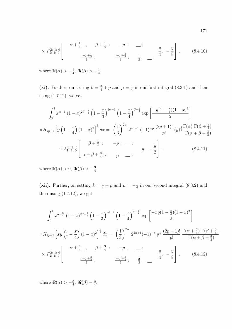
171

× F 2: 1: 02: 1; 0

α + 14

, β + 14

: −p ; ;

α+β+ 12

2,

α+β+ 32

2: 1

2; ;

y

4, − y

8

, (8.4.10)

where <(α) > −14, <(β) > −1

4.

(xi). Further, on setting k = 34

+ p and µ = 14

in our first integral (8.3.1) and then

using (1.7.12), we get

∫ 1

0

xα−1 (1− x)2β− 12

(1− x

3

)2α−1 (1− x

4

)β− 34

exp

[−y(1− x4)(1− x)2

2

]

×H2p+1

[y(

1− x

4

)(1− x)2

] 12dx =

(1

3

)2α

22α+1 (−1)−p(2p+ 1)!

p!(y)

12

Γ(α) Γ(β + 34)

Γ(α + β + 34)

× F 1: 1: 01: 1; 0

β + 34

: −p ; ;

α + β + 34

: 32; ;

y, − y

2

, (8.4.11)

where <(α) > 0, <(β) > −34.

(xii). Further, on setting k = 14

+ p and µ = −14

in our second integral (8.3.2) and

then using (1.7.12), we get

∫ 1

0

xα−34 (1− x)2β− 1

2

(1− x

3

)2α−1 (1− x

4

)β− 34

exp

[−xy(1− x4)(1− x)2

2

]

×H2p+1

[xy(

1− x

4

)(1− x)2

] 12dx =

(1

3

)2α

22α+1(−1)−p y12

(2p+ 1)!

p!

Γ(α + 34) Γ(β + 3

4)

Γ(α + β + 32)

× F 2: 1: 02: 1; 0

α + 34

, β + 34

: −p ; ;

α+β+ 32

2,

α+β+ 52

2: 3

2; ;

y

4, − y

8

, (8.4.12)

where <(α) > −34, <(β)− 3

4.

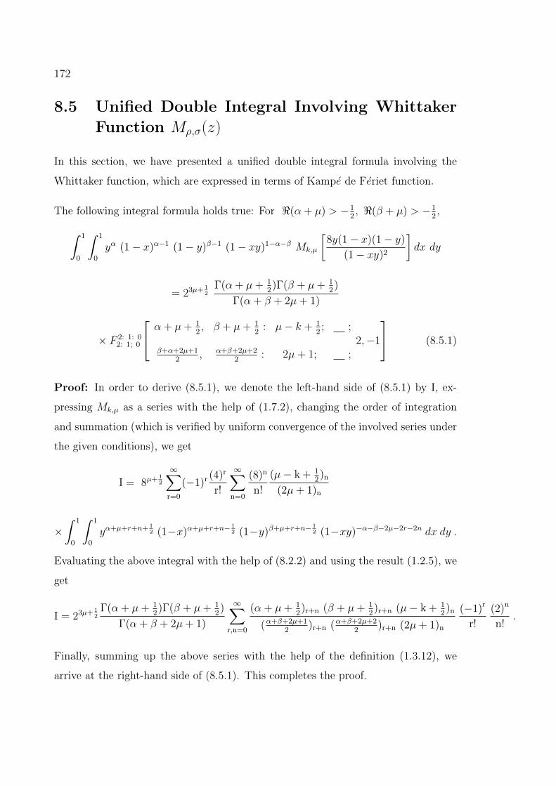
172

8.5 Unified Double Integral Involving Whittaker

Function Mρ,σ(z)

In this section, we have presented a unified double integral formula involving the

Whittaker function, which are expressed in terms of Kampe de Feriet function.

The following integral formula holds true: For <(α + µ) > −12, <(β + µ) > −1

2,∫ 1

0

∫ 1

0

yα (1− x)α−1 (1− y)β−1 (1− xy)1−α−β Mk,µ

[8y(1− x)(1− y)

(1− xy)2

]dx dy

= 23µ+ 12

Γ(α + µ+ 12)Γ(β + µ+ 1

2)

Γ(α + β + 2µ+ 1)

× F 2: 1: 02: 1; 0

α + µ+ 12, β + µ+ 1

2: µ− k + 1

2; ;

β+α+2µ+12

, α+β+2µ+22

: 2µ+ 1; ;2,−1

(8.5.1)

Proof: In order to derive (8.5.1), we denote the left-hand side of (8.5.1) by I, ex-

pressing Mk,µ as a series with the help of (1.7.2), changing the order of integration

and summation (which is verified by uniform convergence of the involved series under

the given conditions), we get

I = 8µ+ 12

∞∑r=0

(−1)r (4)r

r!

∞∑n=0

(8)n

n!

(µ− k + 12)n

(2µ+ 1)n

×∫ 1

0

∫ 1

0

yα+µ+r+n+ 12 (1−x)α+µ+r+n− 1

2 (1−y)β+µ+r+n− 12 (1−xy)−α−β−2µ−2r−2n dx dy .

Evaluating the above integral with the help of (8.2.2) and using the result (1.2.5), we

get

I = 23µ+ 12

Γ(α + µ+ 12)Γ(β + µ+ 1

2)

Γ(α + β + 2µ+ 1)

∞∑r,n=0

(α + µ+ 12)r+n (β + µ+ 1

2)r+n (µ− k + 1

2)n

(α+β+2µ+12

)r+n (α+β+2µ+22

)r+n (2µ+ 1)n

(−1)r

r!

(2)n

n!.

Finally, summing up the above series with the help of the definition (1.3.12), we

arrive at the right-hand side of (8.5.1). This completes the proof.

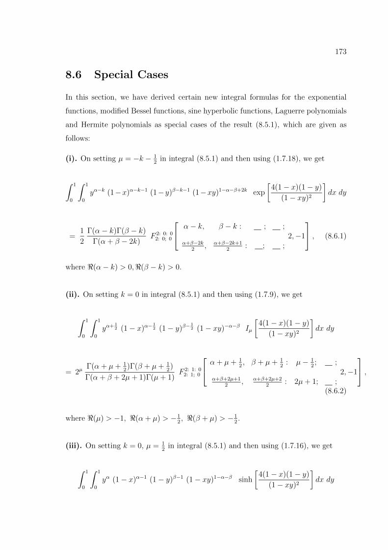
173

8.6 Special Cases

In this section, we have derived certain new integral formulas for the exponential

functions, modified Bessel functions, sine hyperbolic functions, Laguerre polynomials

and Hermite polynomials as special cases of the result (8.5.1), which are given as

follows:

(i). On setting µ = −k − 12

in integral (8.5.1) and then using (1.7.18), we get

∫ 1

0

∫ 1

0

yα−k (1−x)α−k−1 (1−y)β−k−1 (1−xy)1−α−β+2k exp

[4(1− x)(1− y)

(1− xy)2

]dx dy

=1

2

Γ(α− k)Γ(β − k)

Γ(α + β − 2k)F 2: 0: 0

2: 0; 0

α− k, β − k : ; ;

α+β−2k2

, α+β−2k+12

: ; ;2,−1

, (8.6.1)

where <(α− k) > 0,<(β − k) > 0.

(ii). On setting k = 0 in integral (8.5.1) and then using (1.7.9), we get

∫ 1

0

∫ 1

0

yα+ 12 (1− x)α−

12 (1− y)β−

12 (1− xy)−α−β Iµ

[4(1− x)(1− y)

(1− xy)2

]dx dy

= 2µΓ(α + µ+ 1

2)Γ(β + µ+ 1

2)

Γ(α + β + 2µ+ 1)Γ(µ+ 1)F 2: 1: 0

2: 1; 0

α + µ+ 12, β + µ+ 1

2: µ− 1

2; ;

α+β+2µ+12

, α+β+2µ+22

: 2µ+ 1; ;2,−1

,(8.6.2)

where <(µ) > −1, <(α + µ) > −12, <(β + µ) > −1

2.

(iii). On setting k = 0, µ = 12

in integral (8.5.1) and then using (1.7.16), we get

∫ 1

0

∫ 1

0

yα (1− x)α−1 (1− y)β−1 (1− xy)1−α−β sinh

[4(1− x)(1− y)

(1− xy)2

]dx dy

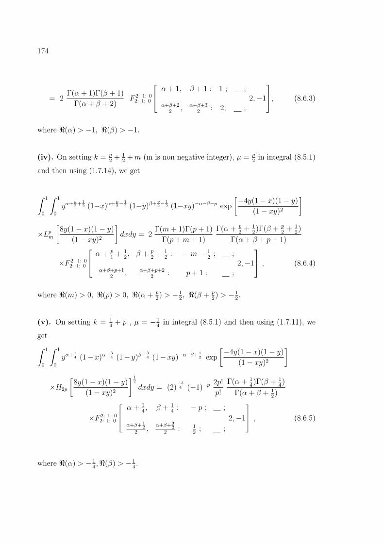
174

= 2Γ(α + 1)Γ(β + 1)

Γ(α + β + 2)F 2: 1: 0

2: 1; 0

α + 1, β + 1 : 1 ; ;

α+β+22

, α+β+32

: 2; ;2,−1

, (8.6.3)

where <(α) > −1, <(β) > −1.

(iv). On setting k = p2

+ 12

+m (m is non negative integer), µ = p2

in integral (8.5.1)

and then using (1.7.14), we get

∫ 1

0

∫ 1

0

yα+ p2

+ 12 (1−x)α+ p

2− 1

2 (1−y)β+ p2− 1

2 (1−xy)−α−β−p exp

[−4y(1− x)(1− y)

(1− xy)2

]

×Lpm[

8y(1− x)(1− y)

(1− xy)2

]dxdy = 2

Γ(m+ 1)Γ(p+ 1)

Γ(p+m+ 1)

Γ(α + p2

+ 12)Γ(β + p

2+ 1

2)

Γ(α + β + p+ 1)

×F 2: 1: 02: 1; 0

α + p1

+ 12, β + p

2+ 1

2: −m− 1

2; ;

α+β+p+12

, α+β+p+22

: p+ 1 ; ;2,−1

, (8.6.4)

where <(m) > 0, <(p) > 0, <(α + p2) > −1

2, <(β + p

2) > −1

2.

(v). On setting k = 14

+ p , µ = −14

in integral (8.5.1) and then using (1.7.11), we

get∫ 1

0

∫ 1

0

yα+ 14 (1−x)α−

34 (1− y)β−

34 (1−xy)−α−β+ 1

2 exp

[−4y(1− x)(1− y)

(1− xy)2

]

×H2p

[8y(1− x)(1− y)

(1− xy)2

] 12

dxdy = (2)−34 (−1)−p

2p!

p!

Γ(α + 14)Γ(β + 1

4)

Γ(α + β + 12)

×F 2: 1: 02: 1; 0

α + 14, β + 1

4: − p ; ;

α+β+ 12

2,

α+β+ 32

2: 1

2; ;

2,−1

, (8.6.5)

where <(α) > −14,<(β) > −1

4.

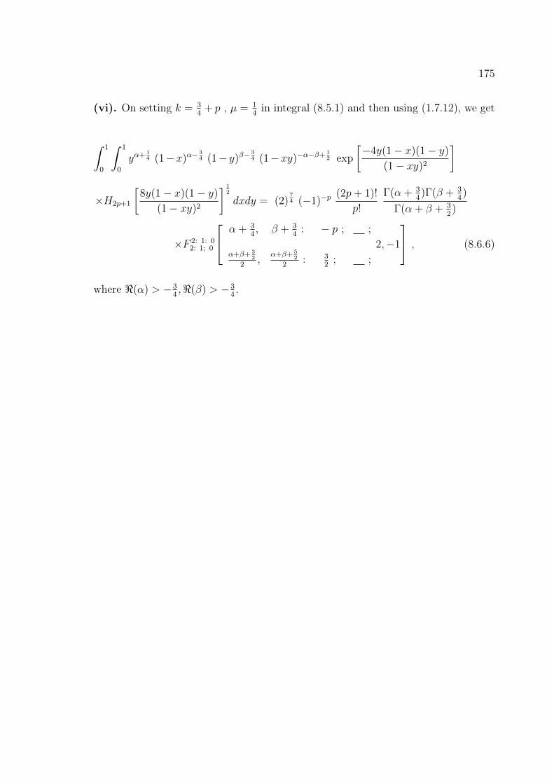
175

(vi). On setting k = 34

+ p , µ = 14

in integral (8.5.1) and then using (1.7.12), we get

∫ 1

0

∫ 1

0

yα+ 14 (1−x)α−

34 (1− y)β−

34 (1−xy)−α−β+ 1

2 exp

[−4y(1− x)(1− y)

(1− xy)2

]

×H2p+1

[8y(1− x)(1− y)

(1− xy)2

] 12

dxdy = (2)74 (−1)−p

(2p+ 1)!

p!

Γ(α + 34)Γ(β + 3

4)

Γ(α + β + 32)

×F 2: 1: 02: 1; 0

α + 34, β + 3

4: − p ; ;

α+β+ 32

2,

α+β+ 52

2: 3

2; ;

2,−1

, (8.6.6)

where <(α) > −34,<(β) > −3

4.

Chapter 9

Certain New Representations ofConfluent HypergeometricFunction and Whittaker Function

9.1 Introduction

The Whittaker function Mk,µ(z) in terms of confluent hypergeometric function (or

Kummer’s function) of first kind (see [150], [175], see also [181]) is defined as

Mk,µ(z) = zµ+ 12 exp

(−z

2

)Φ(µ−k+

1

2; 2µ+1; z), <(µ) > −1

2and <(µ±k) > −1

2.

(9.1.1)

Very recently, Parmar [115] introduced and investigated some fundamental prop-

erties and characteristics of more generalized beta type function B(α,β;m)σ defined by

B(α,β;m)σ (x, y) =

∫ 1

0

tx−1 (1− t)y−11F1

(α; β; − σ

tm(1− t)m

)dt (9.1.2)

(<(σ) > 0, <(x) > 0, <(y) > 0, <(α) > 0, <(β) > 0, <(m) > 0).

When m = 1, (9.1.2) reduces to the well-known generalized beta type function defined

by Ozergin et al. [111]:

B(α,β)σ (x, y) =

∫ 1

0

tx−1 (1− t)y−11F1

(α; β; − σ

t(1− t)

)dt (9.1.3)

(<(σ) > 0, <(x) > 0, <(y) > 0, <(α) > 0, <(β) > 0).

176

177

For α = β, (9.1.3) reduces to

Bσ(x, y) = B(α,α)σ (x, y) =

∫ 1

0

tx−1 (1− t)y−1 exp

(− σ

t(1− t)

)dt (<(σ) > 0),

(9.1.4)

which was introduced by Chaudhry et al. [28] in 1997. Clearly, classical beta function

B(x, y) is given by

B(x, y) = B0(x, y) = B(α,β)0 (x, y).

Using (9.1.4), Chaudhry et al. [29] extended the Gauss hypergeometric function

and confluent hypergeometric function as follows:

Fσ(a, b; c; z) =∞∑n=0

(a)n Bσ(b+ n, c− b)B(b, c− b)

zn

n!(9.1.5)

(σ ≥ 0; |z| < 1; <(c) > <(b) > 0),

Φσ(b; c; z) =∞∑n=0

Bσ(b+ n, c− b)B(b, c− b)

zn

n!(9.1.6)

(σ ≥ 0; <(c) > <(b) > 0)

and gave their Euler’s type integral representation

Fσ(a, b; c; z) =1

B(b, c− b)

∫ 1

0

tb−1 (1−t)c−b−1 (1−zt)−a exp

[− σ

t(1− t)

]dt (9.1.7)

(σ > 0; σ = 0 and | arg(1− z)| < π; <(c) > <(b) > 0),

Φσ(b; c; z) =1

B(b, c− b)

∫ 1

0

tb−1 (1− t)c−b−1 exp

[zt− σ

t(1− t)

]dt (9.1.8)

(σ > 0; σ = 0 and <(c) > <(b) > 0).

By appealing B(α,β)σ (x, y), Ozergin et al. [111] further extended Gauss hypergeometric

function and confluent hypergeometric function by

F (α,β)σ (a, b; c; z) =

∞∑n=0

(a)n B(α,β)σ (b+ n, c− b)B(b, c− b)

zn

n!(9.1.9)

(σ ≥ 0; |z| < 1; <(c) > <(b) > 0, <(α) > 0, <(β) > 0),

178

Φ(α,β)σ (b; c; z) =

∞∑n=0

B(α,β)σ (b+ n, c− b)B(b, c− b)

zn

n!(9.1.10)

(σ ≥ 0; <(c) > <(b) > 0, <(α) > 0, <(β) > 0)

and gave their Euler’s type integral representation

F (α,β)σ (a, b; c; z) =

1

B(b, c− b)

∫ 1

0

tb−1 (1−t)c−b−1 (1−zt)−a 1F1

(α; β; − σ

t(1− t)

)dt

(9.1.11)

(σ > 0; σ = 0 and | arg(1− z)| < π; <(c) > <(b) > 0, <(α) > 0, <(β) > 0),

Φ(α,β)σ (b; c; z) =

1

B(b, c− b)

∫ 1

0

tb−1 (1− t)c−b−1 ezt 1F1

(α; β; − σ

t(1− t)

)dt

(9.1.12)

(σ > 0; σ = 0; <(c) > <(b) > 0, <(α) > 0, <(β) > 0).

By using B(α,β;m)σ (x, y), Parmar [115] defined a new generalization of extended Gauss

hypergeometric function and confluent hypergeometric function as follows:

F (α,β;m)σ (a, b; c; z) =

∞∑n=0

(a)n B(α,β;m)σ (b+ n, c− b)B(b, c− b)

zn

n!(9.1.13)

(σ ≥ 0; |z| < 1; <(c) > <(b) > 0, <(α) > 0, <(β) > 0, <(m) > 0),

Φ(α,β;m)σ (b; c; z) =

∞∑n=0

B(α,β;m)σ (b+ n, c− b)

B(b, c− b)zn

n!(9.1.14)

(σ ≥ 0; <(c) > <(b) > 0, <(α) > 0, <(β) > 0, <(m) > 0),

and gave their Euler’s type integral representation

F (α,β;m)σ (a, b; c; z) =

1

B(b, c− b)

∫ 1

0

tb−1 (1−t)c−b−1 (1−zt)−a 1F1

(α; β; − σ

tm(1− t)m

)dt

(9.1.15)

(σ > 0; σ = 0 and | arg(1− z)| < π; <(c) > <(b) > 0, <(m) > 0),

Φ(α,β;m)σ (b; c; z) =

1

B(b, c− b)

∫ 1

0

tb−1 (1− t)c−b−1 ezt 1F1

(α; β; − σ

tm(1− t)m

)dt

(9.1.16)

179

(σ > 0; σ = 0; <(c) > <(b) > 0, <(m) > 0).

On substituting t = 1 − u in (9.1.16), Parmar [115] obtained the following new

extension of Kummer’s relation for the generalized extended confluent hypergeometric

function of the first kind:

Φ(α,β;m)σ (b; c; z) = exp(z) Φ(α,β;m)

σ (c− b; c;−z). (9.1.17)

For σ = 0, (9.1.17) reduces to the Kummer’s first formula for the classical confluent

hypergeometric function [131].

Afterwards, Srivastava et al. [165] introduced a new generalized Gauss hypergeomet-

ric functions as follows:

F (α,β;m,n)σ (a, b; c; z) =

∞∑k=0

(a)kB

(α,β;m,n)σ (b+ k, c− b)

B(b, c− b)zk

k!(9.1.18)

(|z| < 1; min<(α),<(β),<(m),<(n) > 0; <(c) > <(b) > 0; <(σ) ≥ 0),

where the generalized beta function B(α,β;m,n)σ (x, y) is defined by

B(α,β;m,n)σ (x, y) =

∫ 1

0

tx−1 (1− t)y−11F1

(α; β; − σ

tm(1− t)n

)dt (9.1.19)

(<(σ) ≥ 0; min<(α),<(β),<(x),<(y) > 0; min<(m),<(n) > 0).

On substituting m = n in (9.1.18) and (9.1.19), respectively, we get the extended

Gauss hypergeometric function and extended beta function defined by Parmar [115].

The main object of the present chapter is to introduce a new generalization of ex-

tended confluent hypergeometric function Φ(α,β;m,n)σ (b; c; z) and extended Whittaker

function M(α,β,m,n)σ,k,µ (z). In section 9.2, we have given the definition of new generalized

extended confluent hypergeometric function Φ(α,β;m,n)σ (b; c; z) in terms of extended

beta function, its integral representations and some properties. The derivative for

this generalized extended confluent hypergeometric function Φ(α,β;m,n)σ (b; c; z) is in-

cluded in sections 9.3. Section 9.4 gives some integral transforms and transformation

180

formula of this new generalized extended confluent hypergeometric function. Fur-

ther, in section 9.5, we have defined a new generalized extended Whittaker func-

tion M(α,β,m,n)σ,k,µ (z) by using the generalized extended confluent hypergeometric func-

tion Φ(α,β;m,n)σ (b; c; z), its integral representations and some properties. Section 9.6

gives some integral transforms of this new generalized extended Whittaker function

M(α,β,m,n)σ,k,µ (z). The derivative of the new generalized extended Whittaker function

M(α,β,m,n)σ,k,µ (z) is included in section 9.7. Some recurrence relations for the function

M(α,β,m,n)σ,k,µ (z) are given in the last section 9.8.

9.2 Extended Confluent Hypergeometric Function

Φ(α,β;m,n)σ (b; c; z)

In this section, we have given the definition of the generalized extended confluent

hypergeometric function. An integral representation and Kummer type relation of

this function are also indicated.

Definition 9.2.1. The generalized extended confluent hypergeometric function (for

|z| < 1; min<(α),<(β),<(m),<(n) > 0; <(c) > <(b) > 0; <(σ) ≥ 0) is denoted

by Φ(α,β;m,n)σ (b; c; z) and is defined as follows:

Φ(α,β;m,n)σ (b; c; z) =

∞∑k=0

B(α,β;m,n)σ (b+ k, c− b)

B(b, c− b)zk

k!, (9.2.1)

where B(α,β;m,n)σ is the generalized beta function given by (9.1.19).

Remark 9.2.2. On setting m = n, (9.2.1) reduces to the generalized extended

confluent hypergeometric function defined by Parmar [115], which further for n = 1

gives the known extension of the confluent hypergeometric function given by Ozergin

et al. [111]. Further, if we set α = β and m = n in (9.2.1) then we get the generalized

confluent hypergeometric function defined by Lee et al. [97] and if we put α = β and

m = n = 1 in (9.2.1) then we obtain the extended confluent hypergeometric function

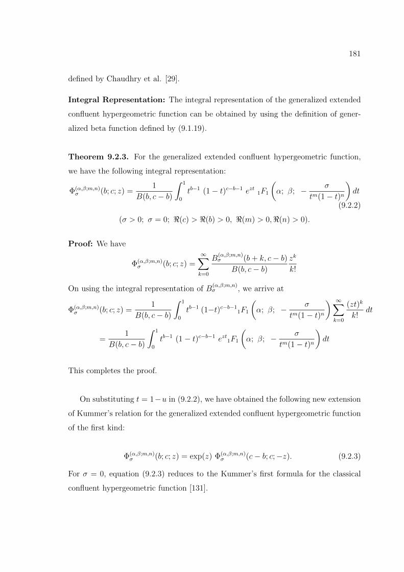
181

defined by Chaudhry et al. [29].

Integral Representation: The integral representation of the generalized extended

confluent hypergeometric function can be obtained by using the definition of gener-

alized beta function defined by (9.1.19).

Theorem 9.2.3. For the generalized extended confluent hypergeometric function,

we have the following integral representation:

Φ(α,β;m,n)σ (b; c; z) =

1

B(b, c− b)

∫ 1

0

tb−1 (1− t)c−b−1 ezt 1F1

(α; β; − σ

tm(1− t)n

)dt

(9.2.2)

(σ > 0; σ = 0; <(c) > <(b) > 0, <(m) > 0,<(n) > 0).

Proof: We have

Φ(α,β;m,n)σ (b; c; z) =

∞∑k=0

B(α,β;m,n)σ (b+ k, c− b)

B(b, c− b)zk

k!

On using the integral representation of B(α,β;m,n)σ , we arrive at

Φ(α,β;m,n)σ (b; c; z) =

1

B(b, c− b)

∫ 1

0

tb−1 (1−t)c−b−11F1

(α; β; − σ

tm(1− t)n

) ∞∑k=0

(zt)k

k!dt

=1

B(b, c− b)

∫ 1

0

tb−1 (1− t)c−b−1 ezt1F1

(α; β; − σ

tm(1− t)n

)dt

This completes the proof.

On substituting t = 1−u in (9.2.2), we have obtained the following new extension

of Kummer’s relation for the generalized extended confluent hypergeometric function

of the first kind:

Φ(α,β;m,n)σ (b; c; z) = exp(z) Φ(α,β;m,n)

σ (c− b; c;−z). (9.2.3)

For σ = 0, equation (9.2.3) reduces to the Kummer’s first formula for the classical

confluent hypergeometric function [131].

182

Remark 9.2.4. On taking m = n, (9.2.2) reduces to the integral representation of

the generalized extended confluent hypergeometric function defined by Parmar [115],

which further for n = 1 gives the integral representation of the extended confluent

hypergeometric function given by Ozergin et al. [111]. Further, if we put α = β

and m = n in (9.2.2), we get the integral representation of generalized confluent

hypergeometric function defined by Lee et al. [97] and if we set α = β and m =

n = 1 in (9.2.2), then we obtain the integral representation of extended confluent

hypergeometric function defined by Chaudhry et al. [29].

9.3 The derivatives of Φ(α,β,m,n)σ (b; c; z)

The derivative of generalized extended confluent hypergeometric function Φ(α,β;m,n)σ (b; c; z)

with respect to the variable z in terms of a shift operator is obtained by using the

following formulas:

B(b, c− b) =b

cB(b+ 1, c− b) and (a)n+1 = a(a + 1)n. (9.3.1)

Theorem 9.3.1. For the generalized extended confluent hypergeometric function

Φ(α,β;m,n)σ (b; c; z), the following differentiation formula holds true:

dr

dzr[Φ(α,β;m,n)σ (b; c; z)

]=

(b)r(c)r

Φ(α,β;m,n)σ (b+ r; c+ r; z). (9.3.2)

Proof: Taking the derivative of Φ(α,β;m,n)σ (b; c; z) with respect to z, we obtain

d

dz

[Φ(α,β;m,n)σ (b; c; z)

]=

d

dz

[∞∑r=0

B(α,β;m,n)σ (b+ r, c− b)

B(b, c− b)zr

r!

]

=∞∑r=1

B(α,β;m,n)σ (b+ r, c− b)

B(b, c− b)zr−1

(r − 1)!.

Replacing r by r + 1, we get

d

dz

[Φ(α,β;m,n)σ (b; c; z)

]=b

c

∞∑r=0

B(α,β;m,n)σ (b+ r + 1, c− b)

B(b+ 1, c− b)zr

r!

183

=b

c

[Φ(α,β;m,n)σ (b+ 1; c+ 1; z)

].

In a similar procedure, by induction, we can obtain the desired result.

9.4 Mellin Transforms and Transformation Formula

of Φ(α,β,m,n)σ (b; c; z)

Certain interesting Mellin transforms and a transformation formula for the general-

ized extended confluent hypergeometric function are given in the following theorems:

Theorem 9.4.1. For the generalized extended confluent hypergeometric function,

we have the following Mellin transform representation:∫ ∞0

σs−1 Φ(α,β;m,n)σ (b; c; z)dσ =

Γ(α,β)(s)B(b+ms, c− b+ ns)

B(b, c− b) 1F1(b+ms; c+(m+n)s; z),

(9.4.1)

where 1F1 is the confluent hypergeometric function defined by (1.2.28).

Proof: To obtain Mellin transform, multiply both sides of (9.2.2) by σs−1, and

integrating with respect to σ over the interval [0,∞), and changing the order of

integral, we get∫ ∞0

σs−1 Φ(α,β;m,n)σ (b; c; z)dσ =

1

B(b, c− b)

∫ 1

0

tb−1 (1− t)c−b−1 ezt

×[∫ ∞

0

σs−11F1

(α; β; − σ

tm(1− t)n

)dσ

]dt.

Substitution of u = σtm(1−t)n in the integral then leads to

∫ ∞0

σs−11F1

(α; β; − σ

tm(1− t)n

)dσ =

∫ ∞0

us−1 tms(1− t)ns 1F1(α; β;−u)du

= tms(1− t)ns∫ ∞

0

us−11F1(α; β;−u)du

184

= tms(1− t)nsΓ(α,β)(s),

where Γ(α,β)(s) is the generalized gamma function [111].

Thus we have

=1

B(b, c− b)

∫ 1

0

tb−1 (1− t)c−b−1 ezt[∫ ∞

0

us−11F1 (α; β; − u) du

]dt

=Γ(α,β)(s)

B(b, c− b)

∫ 1

0

tb+ms−1 (1− t)c−b+ns−1 eztdt

=Γ(α,β)(s)B(b+ms, c− b+ ns)

B(b, c− b) 1F1[b+ms; c+ (m+ n)s; z].

This completes the proof.

Corollary 9.4.2. By the Mellin inversion formula, we have the following complex

integral representation for Φ(α,β;m,n)σ (b; c; z):

Φ(α,β;m,n)σ (b; c; z) =

1

2πi

∫ +i∞

−i∞

Γ(α,β)(s)B(b+ms, c− b+ ns)

B(b, c− b) 1F1(b+ms; c+(m+n)s; z)σ−sds.

(9.4.2)

Proof: Taking Mellin inversion of Theorem (9.4.1), we get the required result.

Theorem 9.4.3. For the generalized extended confluent hypergeometric function,

we have the following transformation formula:

Φ(α,β;m,n)σ (b; c; z) = exp(z)Φ(α,β;m,n)

σ (c− b; c;−z). (9.4.3)

Proof: Using the definition of the generalized extended confluent hypergeometric

function, we have

Φ(α,β;m,n)σ (b; c; z) =

1

B(b, c− b)

∫ 1

0

tb−1 (1− t)c−b−1 ezt 1F1

(α; β; − σ

tm(1− t)n

)dt

Replacing t by t− 1, we get the result.

185

Remark 9.4.4. For m = n, (9.4.3) reduces to the extended Kummar’s first formula

defined by Parmar [115]. Clearly, for σ = 0, (9.4.3) reduces to the well known

Kummer’s first formula for the classical confluent hypergeometric function 1F1.

9.5 Extended Whittaker Function M(α,β,m,n)σ,k,µ (z)

In this section, we have given the definition of the generalized extended Whittaker

function in terms of generalized extended confluent hypergeometric function. Some

integral representations and a relation of this function are also derived.

Definition 9.5.1. The generalized extended Whittaker function for σ ≥ 0, m ≥ 1,

n ≥ 1, <(α) > 0 and <(β) > 0, denoted by M(α,β;m,n)σ,k,µ (z) and is defined as

M(α,β;m,n)σ,k,µ (z) = zµ+ 1

2 exp(−z

2

)Φ(α,β;m,n)σ (µ− k +

1

2; 2µ+ 1; z), (9.5.1)

where <(µ) > −12, <(µ±k) > −1

2and Φ

(α,β;m,n)σ is the generalized extended confluent

hypergeometric function of the first kind defined by (9.2.2).

On setting m = n = 1 in (9.5.1), we have obtained the following (presumably) a new

representation of the extended Whittaker function:

M(α,β;1,1)σ,k,µ (z) = M

(α,β)σ,k,µ (z) = zµ+ 1

2 exp(−z

2

)Φ(α,β)σ (µ−k+

1

2; 2µ+ 1; z), (9.5.2)

where <(µ) > −12, <(µ± k) > −1

2.

Remark 9.5.2. On setting m = n in (9.5.1), we have obtained the generalized

extended Whittaker function defined by Choi et al. [26]. Further, on setting α =

β, m = n in (9.5.1), we get the extended Whittaker function given by Khan and

Ghayasuddin [74], which further for n = 1 gives the extended Whittaker function

due to Nagar et al. [103]. For σ = 0, (9.5.1) reduces to the classical Whittaker

function defined by (9.1.1).

Integral Representations: Certain interesting integral representations of the gen-

eralized extended Whittaker function M(α,β;m,n)σ,k,µ (z) are given in the following theorem:

186

Theorem 9.5.3. Suppose that

σ > 0; σ = 0 and <(µ) > <(µ± k) > −1

2, <(m) > 0,<(n) > 0.

Each of the following integral formulas holds true:

M(α,β;m,n)σ,k,µ (z) =

zµ+ 12 exp(− z

2)

B(µ− k + 12, µ+ k + 1

2)

×∫ 1

0

tµ−k−12 (1− t)µ+k− 1

2 ezt 1F1

(α; β; − σ

tm(1− t)n

)dt; (9.5.3)

M(α,β;m,n)σ,k,µ (z) =

zµ+ 12 exp( z

2)

B(µ− k + 12, µ+ k + 1

2)

×∫ 1

0

uµ+k− 12 (1−u)µ−k−

12 e−zu 1F1

(α; β; − σ

un(1− u)m

)dt;

(9.5.4)

M(α,β;m,n)σ,k,µ (z) =

(q − p)−2µ zµ+ 12 exp(− z

2)

B(µ− k + 12, µ+ k + 1

2)

×∫ q

p

(u−p)µ−k−12 (q−u)µ+k− 1

2 exp

[z(u− p)(q − p)

]1F1

(α; β; − σ (q − p)m+n

(u− p)m(q − u)n

)du;

(9.5.5)

M(α,β;m,n)σ,k,µ (z) =

exp(− z

2

)zµ+ 1

2

B(µ− k + 12, µ+ k + 1

2)

×∫ ∞

0

uµ−k−12 (1 + u)−(2µ+1) exp

(zu

1 + u

)1F1

(α; β; − σ (1 + u)m+n

um

)du;

(9.5.6)

M(α,β;m,n)σ,k,µ (z) =

2−2µ zµ+ 12

B(µ− k + 12, µ+ k + 1

2)

×∫ 1

−1

(1 + u)µ−k−12 (1− u)µ+k− 1

2 exp(zu

2

)1F1

(α; β; − 2m+n σ

(1 + u)m(1− u)n

)du.

(9.5.7)

187

Proof: The use of (9.2.2) in (9.5.1) is seen to yield the integral representation (9.5.3).

Setting t = 1− u, t = u−pq−p and t = u

1+uin (9.5.3) yield (9.5.4),(9.5.5),(9.5.6) respec-

tively. Setting q = 1 and p = −1 in (9.5.5) gives (9.5.7).

Remark 9.5.4. On setting m = n in (9.5.3), (9.5.4), (9.5.5), (9.5.6) and (9.5.7), we

have obtained the integral representations of generalized extended Whittaker func-

tion defined by Choi et al. [26], which, on further setting α = β correspond with

the integral representations for the extended Whittaker function given by Khan and

Ghayasuddin [74]. The case α = β, m = n = 1 of (9.5.3), (9.5.4), (9.5.5), (9.5.6)

and (9.5.7) is seen to yield the integral representations of the generalized extended

Whittaker function due to Nagar et al. [103].

Remark 9.5.5. On using (9.2.2) in the equation (9.5.4), we get

M(α,β;m,n)σ,k,µ (z) = zµ+ 1

2 exp(−z

2

)Φ(α,β;m,n)σ (µ+ k +

1

2; 2µ+ 1;−z), (9.5.8)

Thus it is seen that the generalized extended Whittaker function can also be ex-

pressed by (9.5.8).

Theorem 9.5.6. The following relation holds true:

M(α,β;m,n)σ,k,µ (−z) = (−1)µ+ 1

2 M(α,β;m,n)σ,−k,µ (z). (9.5.9)

(σ > 0; σ = 0 and <(µ) > <(µ± k) > −1

2, <(α) > 0,<(β) > 0).

Proof: Replacing z by −z in (9.5.1), we get

M(α,β;m)σ,k,µ (−z) = (−z)µ+ 1

2 exp(z

2

)Φ(α,β;m)σ (µ− k +

1

2; 2µ+ 1;−z). (9.5.10)

Now using (9.2.3) in (9.5.10) and then writing the resulting expression by using

(9.5.1), we get the desired result.

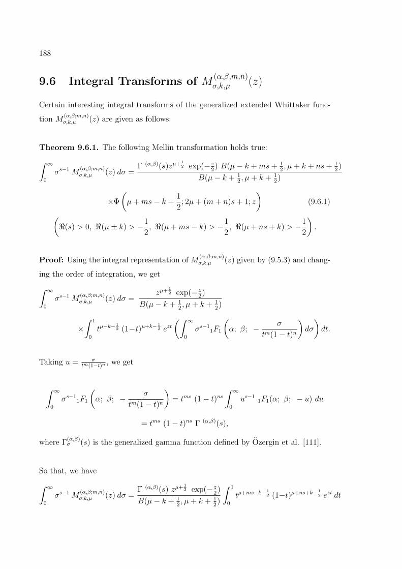
188

9.6 Integral Transforms of M(α,β,m,n)σ,k,µ (z)

Certain interesting integral transforms of the generalized extended Whittaker func-

tion M(α,β;m,n)σ,k,µ (z) are given as follows:

Theorem 9.6.1. The following Mellin transformation holds true:∫ ∞0

σs−1 M(α,β;m,n)σ,k,µ (z) dσ =

Γ (α,β)(s)zµ+ 12 exp(− z

2) B(µ− k +ms+ 1

2, µ+ k + ns+ 1

2)

B(µ− k + 12, µ+ k + 1

2)

×Φ

(µ+ms− k +

1

2; 2µ+ (m+ n)s+ 1; z

)(9.6.1)(

<(s) > 0, <(µ± k) > −1

2, <(µ+ms− k) > −1

2, <(µ+ ns+ k) > −1

2

).

Proof: Using the integral representation of M(α,β;m,n)σ,k,µ (z) given by (9.5.3) and chang-

ing the order of integration, we get∫ ∞0

σs−1 M(α,β;m,n)σ,k,µ (z) dσ =

zµ+ 12 exp(− z

2)

B(µ− k + 12, µ+ k + 1

2)

×∫ 1

0

tµ−k−12 (1−t)µ+k− 1

2 ezt(∫ ∞

0

σs−11F1

(α; β; − σ

tm(1− t)n

)dσ

)dt.

Taking u = σtm(1−t)n , we get

∫ ∞0

σs−11F1

(α; β; − σ

tm(1− t)n

)= tms (1− t)ns

∫ ∞0

us−11F1(α; β; − u) du

= tms (1− t)ns Γ (α,β)(s),

where Γ(α,β)σ (s) is the generalized gamma function defined by Ozergin et al. [111].

So that, we have∫ ∞0

σs−1 M(α,β;m,n)σ,k,µ (z) dσ =

Γ (α,β)(s) zµ+ 12 exp(− z

2)

B(µ− k + 12, µ+ k + 1

2)

∫ 1

0

tµ+ms−k− 12 (1−t)µ+ns+k− 1

2 ezt dt

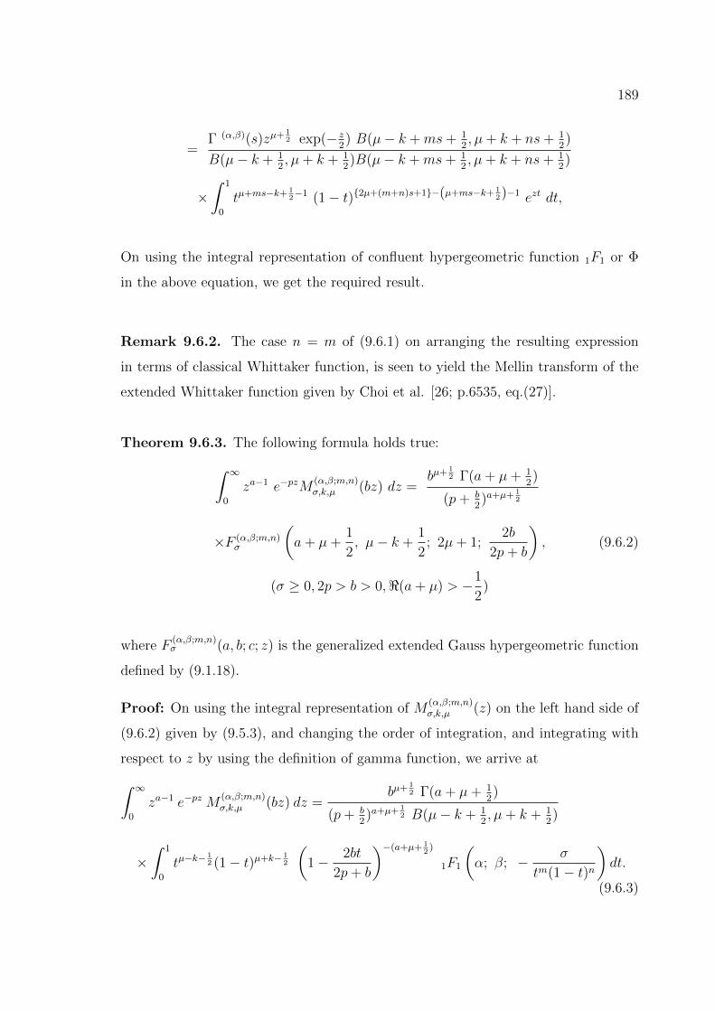
189

=Γ (α,β)(s)zµ+ 1

2 exp(− z2) B(µ− k +ms+ 1

2, µ+ k + ns+ 1

2)

B(µ− k + 12, µ+ k + 1

2)B(µ− k +ms+ 1

2, µ+ k + ns+ 1

2)

×∫ 1

0

tµ+ms−k+ 12−1 (1− t)2µ+(m+n)s+1−(µ+ms−k+ 1

2)−1 ezt dt,

On using the integral representation of confluent hypergeometric function 1F1 or Φ

in the above equation, we get the required result.

Remark 9.6.2. The case n = m of (9.6.1) on arranging the resulting expression

in terms of classical Whittaker function, is seen to yield the Mellin transform of the

extended Whittaker function given by Choi et al. [26; p.6535, eq.(27)].

Theorem 9.6.3. The following formula holds true:∫ ∞0

za−1 e−pzM(α,β;m,n)σ,k,µ (bz) dz =

bµ+ 12 Γ(a+ µ+ 1

2)

(p+ b2)a+µ+ 1

2

×F (α,β;m,n)σ

(a+ µ+

1

2, µ− k +

1

2; 2µ+ 1;

2b

2p+ b

), (9.6.2)

(σ ≥ 0, 2p > b > 0,<(a+ µ) > −1

2)

where F(α,β;m,n)σ (a, b; c; z) is the generalized extended Gauss hypergeometric function

defined by (9.1.18).

Proof: On using the integral representation of M(α,β;m,n)σ,k,µ (z) on the left hand side of

(9.6.2) given by (9.5.3), and changing the order of integration, and integrating with

respect to z by using the definition of gamma function, we arrive at∫ ∞0

za−1 e−pz M(α,β;m,n)σ,k,µ (bz) dz =

bµ+ 12 Γ(a+ µ+ 1

2)

(p+ b2)a+µ+ 1

2 B(µ− k + 12, µ+ k + 1

2)

×∫ 1

0

tµ−k−12 (1− t)µ+k− 1

2

(1− 2bt

2p+ b

)−(a+µ+ 12

)

1F1

(α; β; − σ

tm(1− t)n

)dt.

(9.6.3)

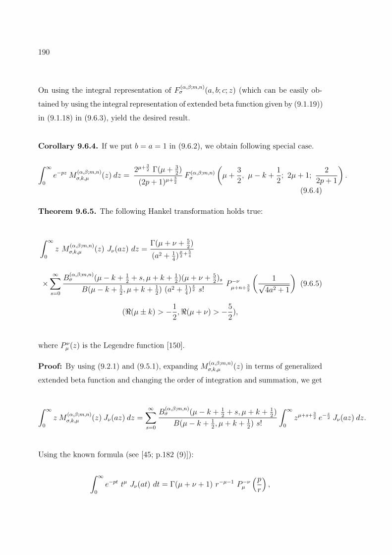
190

On using the integral representation of F(α,β;m,n)σ (a, b; c; z) (which can be easily ob-

tained by using the integral representation of extended beta function given by (9.1.19))

in (9.1.18) in (9.6.3), yield the desired result.

Corollary 9.6.4. If we put b = a = 1 in (9.6.2), we obtain following special case.

∫ ∞0

e−pz M(α,β;m,n)σ,k,µ (z) dz =

2µ+ 32 Γ(µ+ 3

2)

(2p+ 1)µ+ 32

F (α,β;m,n)σ

(µ+

3

2, µ− k +

1

2; 2µ+ 1;

2

2p+ 1

).

(9.6.4)

Theorem 9.6.5. The following Hankel transformation holds true:

∫ ∞0

z M(α,β;m,n)σ,k,µ (z) Jν(az) dz =

Γ(µ+ ν + 52)

(a2 + 14)µ2

+ 54

×∞∑s=0

B(α,β;m,n)σ (µ− k + 1

2+ s, µ+ k + 1

2)(µ+ ν + 5

2)s

B(µ− k + 12, µ+ k + 1

2) (a2 + 1

4)s2 s!

P−νµ+n+ 3

2

(1√

4a2 + 1

)(9.6.5)

(<(µ± k) > −1

2,<(µ+ ν) > −5

2),

where P νµ (z) is the Legendre function [150].

Proof: By using (9.2.1) and (9.5.1), expanding M(α,β;m,n)σ,k,µ (z) in terms of generalized

extended beta function and changing the order of integration and summation, we get

∫ ∞0

z M(α,β;m,n)σ,k,µ (z) Jν(az) dz =

∞∑s=0

B(α,β;m,n)σ (µ− k + 1

2+ s, µ+ k + 1

2)

B(µ− k + 12, µ+ k + 1

2) s!

∫ ∞0

zµ+s+ 32 e−

z2 Jν(az) dz.

Using the known formula (see [45; p.182 (9)]):

∫ ∞0

e−pt tµ Jν(at) dt = Γ(µ+ ν + 1) r−µ−1 P−νµ

(pr

),

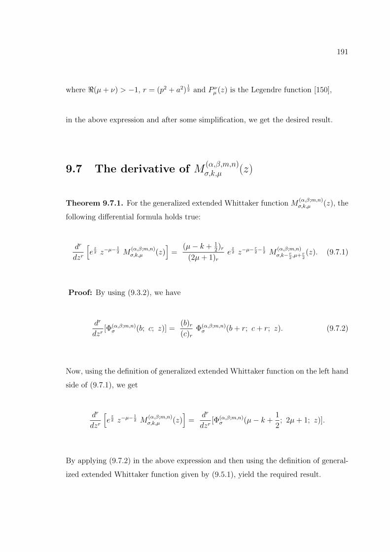
191

where <(µ+ ν) > −1, r = (p2 + a2)12 and P ν

µ (z) is the Legendre function [150],

in the above expression and after some simplification, we get the desired result.

9.7 The derivative of M(α,β,m,n)σ,k,µ (z)

Theorem 9.7.1. For the generalized extended Whittaker function M(α,β;m,n)σ,k,µ (z), the

following differential formula holds true:

dr

dzr

[ez2 z−µ−

12 M

(α,β;m,n)σ,k,µ (z)

]=

(µ− k + 12)r

(2µ+ 1)rez2 z−µ−

r2− 1

2 M(α,β;m,n)σ,k− r

2,µ+ r

2(z). (9.7.1)

Proof: By using (9.3.2), we have

dr

dzr[Φ(α,β;m,n)

σ (b; c; z)] =(b)r(c)r

Φ(α,β;m,n)σ (b+ r; c+ r; z). (9.7.2)

Now, using the definition of generalized extended Whittaker function on the left hand

side of (9.7.1), we get

dr

dzr

[ez2 z−µ−

12 M

(α,β;m,n)σ,k,µ (z)

]=

dr

dzr[Φ(α,β;m,n)

σ (µ− k +1

2; 2µ+ 1; z)].

By applying (9.7.2) in the above expression and then using the definition of general-

ized extended Whittaker function given by (9.5.1), yield the required result.

192

9.8 Recurrence type Relations for M(α,β,m,n)σ,k,µ (z)

Theorem 9.8.1. The following relations for the generalized extended Whittaker

function M(α,β;m,n)σ,k,µ (z) holds true:

(i) (β−α)M(α−1,β;m,n)σ,k,µ (z)+(2α−β)M

(α,β;m,n)σ,k,µ (z)−

σzµ+ 12 exp(− z

2)B(µ−m− k + 1

2, µ− n+ k + 1

2)

B(µ− k + 12, µ+ k + 1

2)

×Φ

(µ−m− k +

1

2; 2µ− (m+ n) + 1; z

)− α M

(α+1,β;m)σ,k,µ (z) = 0; (9.8.1)

(ii) β(β−1)M(α,β−1;m,n)σ,k,µ (z)−β(β−1)M

(α,β;m,n)σ,k,µ (z)

+σβzµ+ 1

2 exp(− z2)B(µ−m− k + 1

2, µ− n+ k + 1

2)

B(µ− k + 12, µ+ k + 1

2)

Φ

(µ−m− k +

1

2; 2µ− (m+ n) + 1; z

)

−σ(β − α)zµ+ 1

2 exp(− z2)B(µ−m− k + 1

2, µ− n+ k + 1

2)

B(µ− k + 12, µ+ k + 1

2)

×Φ

(µ−m− k +

1

2; 2µ− (m+ n) + 1; z

)= 0; (9.8.2)

(iii) (1+α−β)M(α+1,β;m,n)σ,k,µ (z)+(β−1)M

(α,β−1;m,n)σ,k,µ (z) = 0; (9.8.3)

(iv) β M(α,β;m,n)σ,k,µ (z)−β M (α−1,β;m,n)

σ,k,µ (z)+σ zµ+ 1

2 exp(− z2)B(µ−m− k + 1

2, µ− n+ k + 1

2)

B(µ− k + 12, µ+ k + 1

2)

×Φ

(µ−m− k +

1

2; 2µ− (m+ n) + 1; z

)= 0; (9.8.4)

(v) αβ M(α,β;m,n)σ,k,µ (z)−

σβzµ+ 12 exp(− z

2)B(µ−m− k + 1

2, µ− n+ k + 1

2)

B(µ− k + 12, µ+ k + 1

2)

193

×Φ

(µ−m− k +

1

2; 2µ− (m+ n) + 1; z

)

+σ(β − α)zµ+ 1

2 exp(− z2)B(µ−m− k + 1

2, µ− n+ k + 1

2)

B(µ− k + 12, µ+ k + 1

2)

× Φ

(µ−m− k +

1

2; 2µ− (m+ n) + 1; z

)− αβ M (α+1,β;m,n)

σ,k,µ (z) = 0; (9.8.5)

(vi) (α−1)M(α,β+1;m,n)σ,k,µ (z)−

σzµ+ 12 exp(− z

2)B(µ−m− k + 1

2, µ− n+ k + 1

2)

B(µ− k + 12, µ+ k + 1

2)

×Φ

(µ−m− k +

1

2; 2µ− (m+ n) + 1; z

)+(β−α)M

(α−1,β;m,n)σ,k,µ (z)−(β−1)M

(α,β−1;m,n)σ,k,µ (z) = 0.

(9.8.6)

Proof (i): We have the following recurrence relation of the confluent hypergeometric

function 1F1 (see [139; p.19])

(b−a) 1F1(a−1; b; z)+(2a−b) 1F1(a; b; z)+z 1F1(a; b; z)−a 1F1(a+1; b; z) = 0.

(9.8.7)

With the help of above relation (9.8.7), we derive

(β − α) zµ+ 12 exp(− z

2)

B(µ− k + 12, µ+ k + 1

2)

∫ 1

0

tµ−k−12 (1−t)µ+k− 1

2 ezt 1F1

(α− 1; β; − σ

tm(1− t)n

)dt

+(2α− β) zµ+ 1

2 exp(− z2)

B(µ− k + 12, µ+ k + 1

2)

∫ 1

0

tµ−k−12 (1− t)µ+k− 1

2 ezt 1F1

(α; β; − σ

tm(1− t)n

)dt

−σ zµ+ 1

2 exp(− z2)

B(µ− k + 12, µ+ k + 1

2)

∫ 1

0

tµ−m−k−12 (1−t)µ−n+k− 1

2 ezt 1F1

(α; β; − σ

tm(1− t)n

)dt

194

−α zµ+ 1

2 exp(− z2)

B(µ− k + 12, µ+ k + 1

2)

∫ 1

0

tµ−k−12 (1−t)µ+k− 1

2 ezt 1F1

(α + 1; β; − σ

tm(1− t)n

)dt = 0.

By using the integral representations of M(α,β;m)σ,k,µ (z) and Φ in the above expression, we

get our first relation (9.8.1). Similarly, we can derive (9.8.2), (9.8.3), (9.8.4), (9.8.5)

and (9.8.6) by using the following recurrence relations of 1F1 (see [139; p.19]):

b(b−1) 1F1(a; b−1; z)−b(b−1) 1F1(a; b; z)−bz 1F1(a; b; z)+(b−a)z 1F1(a; b+1; z) = 0;

(9.8.8)

(1 + a− b) 1F1(a; b; z)− a 1F1(a+ 1; b; z) + (b− 1) 1F1(a; b− 1; z) = 0; (9.8.9)

b 1F1(a; b; z)− b 1F1(a− 1; b; z)− z 1F1(a; b+ 1; z) = 0; (9.8.10)

ab 1F1(a; b; z) + bz 1F1(a; b; z)− (b− a)z 1F1(a; b+ 1; z)− ab 1F1(a+ 1; b; z) = 0;

(9.8.11)

(a−1) 1F1(a; b; z)+z 1F1(a; b; z)+(b−a) 1F1(a−1; b; z)−(b−1) 1F1(a; b−1; z) = 0.

(9.8.12)

Chapter 10

Evaluation of Integrals Associatedwith Multiple (multiindex)Mittag-Leffler Function

10.1 Introduction

As a result of researchers and scientists increasing interest in pure as well as applied

mathematics in nonconventional models, particularly those using fractional calculus,

Mittag-Leffler functions have recently caught the interest of the scientific commu-

nity. The Mittag-Leffler function was introduced by Gosta Mittag-Leffler [100] in

connection with his method of summation of some divergent series. Its importance

is realised during the last two decades due to its involvement in the problems of

physics, chemistry, biology, engineering and applied sciences. Mittag-Leffler function

naturally occurs as the solution of fractional order differential equation or fractional

order integral equations. The Mittag-Leffler function is an important function that

finds widespread use in the world of fractional calculus. Just as the exponential

naturally arises out of the solution to integer order differential equations, the Mittag-

Leffler function plays an analogous role in the solution of noninteger order differential

equations. The Mittag-Leffler function appears also in the solution of the fractional

master equation. Such an equation characterizes the renewal processes with rewards

modeling by the random walk model known as continuous time random walk. The

question arises for the solution of differential equations with the fractional deriva-

195

196

tives of the Riemann-Liouville type of arbitrary order α, < (α > 0) and n boundary

conditions n = <(α + 1) in the form of the values at the initial point (these initial

condition are so called Cauchy-type conditions). Its was observe that the suitable

class of functions, the solution is unique and is represented though Mittag-Leffler

function. Although some generalization of Mittag-Leffler function have been given

by a number of authors, (see [116], [134], [146] and [148]). The Mittag-Leffler function

plays an important role in pure as well as applied mathematics which was studied by

many authors for many different point of view.

Recently, Singh and Rawat [149] have established some integrals involving the product

of generalized Mittag-Leffler function with Jacobi polynomial, which are expressed in

terms of generalized hypergeometric function. Very recently, Choudhary and Choud-

hary [25] further established some more integrals associated with generalized Mittag-

Leffler functions. Motivated by the above mentioned work, in the present chapter, we

have established some new integrals associated with multiple (multiindex) Mittag-

Leffler function.

In the present chapter firstly, we have investigated some interesting integrals in-

volving the product of multiple (multiindex) Mittag-Leffler function E( 1ρi

),(µi)(z) with

Jacobi polynomial P(α,β)n (z) in section 10.2, which are expressed in terms of gener-

alized hypergeometric function. Some interesting integrals involving the product of

multiple (multiindex) Mittag-Leffler function with Bessel Maitland function, Legen-

dre function, Hermite polynomial, Hypergeometric function and Generalized hyperge-

ometric function are given in section 10.3, 10.4, 10.5, 10.6 and 10.7 respectively. The

results associated with this chapter, involving multiple (multiindex) Mittag-Leffler

function is applied to many different engineering discipline including signal process-

ing, control engineering and many other field such as biology and neuro sciences.

Fractional operators are the generalization of differentiation and integration of inte-

ger order calculus that allow us to present an accurate description of real systems

which includes a combination of multi-disciplinary fields of geometry. A fractional

generalization of the Poisson probability distribution (which is called Mittag-Leffler

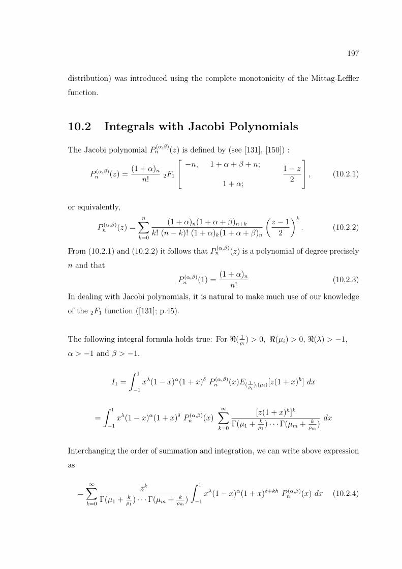
197

distribution) was introduced using the complete monotonicity of the Mittag-Leffler

function.

10.2 Integrals with Jacobi Polynomials

The Jacobi polynomial P(α,β)n (z) is defined by (see [131], [150]) :

P (α,β)n (z) =

(1 + α)nn!

2F1

−n, 1 + α + β + n;

1 + α;

1− z2

, (10.2.1)

or equivalently,

P (α,β)n (z) =

n∑k=0

(1 + α)n(1 + α + β)n+k

k! (n− k)! (1 + α)k(1 + α + β)n

(z − 1

2

)k. (10.2.2)

From (10.2.1) and (10.2.2) it follows that P(α,β)n (z) is a polynomial of degree precisely

n and that

P (α,β)n (1) =

(1 + α)nn!

(10.2.3)

In dealing with Jacobi polynomials, it is natural to make much use of our knowledge

of the 2F1 function ([131]; p.45).

The following integral formula holds true: For <( 1ρi

) > 0, <(µi) > 0, <(λ) > −1,

α > −1 and β > −1.

I1 =

∫ 1

−1

xλ(1− x)α(1 + x)δ P (α,β)n (x)E( 1

ρi),(µi)

[z(1 + x)h] dx

=

∫ 1

−1

xλ(1− x)α(1 + x)δ P (α,β)n (x)

∞∑k=0

[z(1 + x)h]k

Γ(µ1 + kρ1

) · · ·Γ(µm + kρm

)dx

Interchanging the order of summation and integration, we can write above expression

as

=∞∑k=0

zk

Γ(µ1 + kρ1

) · · ·Γ(µm + kρm

)

∫ 1

−1

xλ(1− x)α(1 + x)δ+kh P (α,β)n (x) dx (10.2.4)

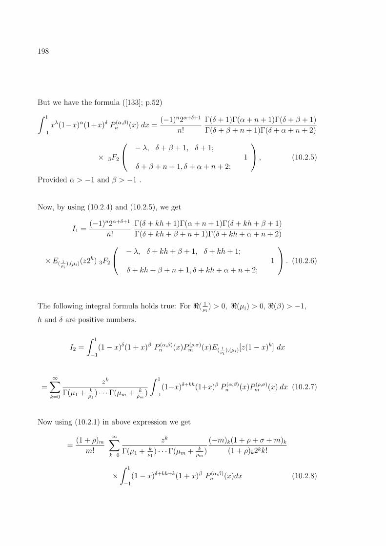
198

But we have the formula ([133]; p.52)∫ 1

−1

xλ(1−x)α(1+x)δ P (α,β)n (x) dx =

(−1)n2α+δ+1

n!

Γ(δ + 1)Γ(α + n+ 1)Γ(δ + β + 1)

Γ(δ + β + n+ 1)Γ(δ + α + n+ 2)

× 3F2

− λ, δ + β + 1, δ + 1;1

δ + β + n+ 1, δ + α + n+ 2;

, (10.2.5)

Provided α > −1 and β > −1 .

Now, by using (10.2.4) and (10.2.5), we get

I1 =(−1)n2α+δ+1

n!

Γ(δ + kh+ 1)Γ(α + n+ 1)Γ(δ + kh+ β + 1)

Γ(δ + kh+ β + n+ 1)Γ(δ + kh+ α + n+ 2)

×E( 1ρi

),(µi)(z2h) 3F2

− λ, δ + kh+ β + 1, δ + kh+ 1;1

δ + kh+ β + n+ 1, δ + kh+ α + n+ 2;

. (10.2.6)

The following integral formula holds true: For <( 1ρi

) > 0, <(µi) > 0, <(β) > −1,

h and δ are positive numbers.

I2 =

∫ 1

−1

(1− x)δ(1 + x)β P (α,β)n (x)P (ρ,σ)

m (x)E( 1ρi

),(µi)[z(1− x)h] dx

=∞∑k=0

zk

Γ(µ1 + kρ1

) · · ·Γ(µm + kρm

)

∫ 1

−1

(1−x)δ+kh(1+x)β P (α,β)n (x)P (ρ,σ)

m (x) dx (10.2.7)

Now using (10.2.1) in above expression we get

=(1 + ρ)mm!

∞∑k=0

zk

Γ(µ1 + kρ1

) · · ·Γ(µm + kρm

)

(−m)k(1 + ρ+ σ +m)k(1 + ρ)k2kk!

×∫ 1

−1

(1− x)δ+kh+k(1 + x)β P (α,β)n (x)dx (10.2.8)

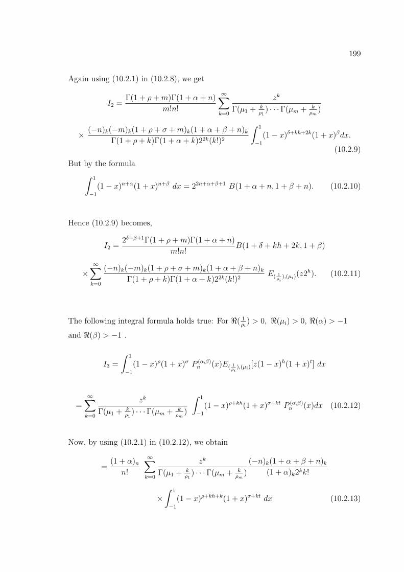
199

Again using (10.2.1) in (10.2.8), we get

I2 =Γ(1 + ρ+m)Γ(1 + α + n)

m!n!

∞∑k=0

zk

Γ(µ1 + kρ1

) · · ·Γ(µm + kρm

)

× (−n)k(−m)k(1 + ρ+ σ +m)k(1 + α + β + n)kΓ(1 + ρ+ k)Γ(1 + α + k)22k(k!)2

∫ 1

−1

(1− x)δ+kh+2k(1 + x)βdx.

(10.2.9)

But by the formula∫ 1

−1

(1− x)n+α(1 + x)n+β dx = 22n+α+β+1 B(1 + α + n, 1 + β + n). (10.2.10)

Hence (10.2.9) becomes,

I2 =2δ+β+1Γ(1 + ρ+m)Γ(1 + α + n)

m!n!B(1 + δ + kh+ 2k, 1 + β)

×∞∑k=0

(−n)k(−m)k(1 + ρ+ σ +m)k(1 + α + β + n)kΓ(1 + ρ+ k)Γ(1 + α + k)22k(k!)2

E( 1ρi

),(µi)(z2h). (10.2.11)

The following integral formula holds true: For <( 1ρi

) > 0, <(µi) > 0, <(α) > −1

and <(β) > −1 .

I3 =

∫ 1

−1

(1− x)ρ(1 + x)σ P (α,β)n (x)E( 1

ρi),(µi)

[z(1− x)h(1 + x)t] dx

=∞∑k=0

zk

Γ(µ1 + kρ1

) · · ·Γ(µm + kρm

)

∫ 1

−1

(1− x)ρ+kh(1 + x)σ+kt P (α,β)n (x)dx (10.2.12)

Now, by using (10.2.1) in (10.2.12), we obtain

=(1 + α)n

n!

∞∑k=0

zk

Γ(µ1 + kρ1

) · · ·Γ(µm + kρm

)

(−n)k(1 + α + β + n)k(1 + α)k2kk!

×∫ 1

−1

(1− x)ρ+kh+k(1 + x)σ+kt dx (10.2.13)

200

Using (10.2.10) in (10.2.13), we get

I3 =2ρ+σ+1(1 + α)n

n!

∞∑k=0

(−n)k(1 + α + β + n)k(1 + α)k k!

E( 1ρi

),(µi)(z2h+t)

×B(1 + ρ+ kh+ k, 1 + σ + tk). (10.2.14)

The following integral formula holds true: For <( 1ρi

) > 0, <(µi) > 0, <(α) > −1

and <(β) > −1 .

I4 =

∫ 1

−1

(1− x)ρ(1 + x)σ P (α,β)n (x)E( 1

ρi),(µi)

[z(1− x)h(1 + x)−t] dx

=∞∑k=0

zk

Γ(µ1 + kρ1

) · · ·Γ(µm + kρm

)

∫ 1

−1

(1− x)ρ+kh(1 + x)σ−kt P (α,β)n (x)dx. (10.2.15)

Now, by using (10.2.10) in (10.2.15), we obtain

=(1 + α)n

n!

∞∑k=0

zk

Γ(µ1 + kρ1

) · · ·Γ(µm + kρm

)

(−n)k(1 + α + β + n)k(1 + α)k2kk!

×∫ 1

−1

(1− x)ρ+kh+k(1 + x)σ−kt dx. (10.2.16)

Using (10.2.10) in (10.2.16), we get

I4 =2ρ+σ+1(1 + α)n

n!

∞∑k=0

(−n)k(1 + α + β + n)k(1 + α)k k!

E( 1ρi

),(µi)(z2h−t)

×B(1 + ρ+ kh+ k, 1 + σ − tk). (10.2.17)

The following integral formula holds true: For <( 1ρi

) > 0, <(µi) > 0, <(α) > −1

and <(β) > −1 .

I5 =

∫ 1

−1

(1− x)ρ(1 + x)σ P (α,β)n (x)E( 1

ρi),(µi)

[z(1 + x)−h] dx

201

=∞∑k=0

zk

Γ(µ1 + kρ1

) · · ·Γ(µm + kρm

)

∫ 1

−1

(1− x)ρ(1 + x)σ−kh P (α,β)n (x)dx (10.2.18)

Now, by using (10.2.1) in (10.2.18), we obtain

=(1 + α)n

n!

∞∑k=0

zk

Γ(µ1 + kρ1

) · · ·Γ(µm + kρm

)

(−n)k(1 + α + β + n)k(1 + α)k2kk!

×∫ 1

−1

(1− x)ρ+k(1 + x)σ−kh dx. (10.2.19)

Using (10.2.10) in (10.2.19), we get

I5 =2ρ+σ+1(1 + α)n

n!

∞∑k=0

(−n)k(1 + α + β + n)k(1 + α)k k!

E( 1ρi

),(µi)(z2−h)

×B(1 + ρ+ k, 1 + σ − kh). (10.2.20)

SPECIAL CASES

(i) If we replace δ by λ − 1 and put α = β = ρ = σ = 0 in equation (10.2.7), then

the integral I2 transforms into the following integral involving Legendre polynomial

(see [131], [150]),

I6 =

∫ 1

−1

(1− x)λ−1 Pn(x)Pm(x)E( 1ρi

),(µi)[z(1− x)h] dx

= 2λ∞∑k=0

(−n)k(−m)k(1 +m)k(1 + n)k

(k!)2(k!)2E( 1

ρi),(µi)

(z2h)B(λ+ kh+ 2k, 1). (10.2.21)

(ii) If α = β = 0 and ρ is replaced by ρ−1 and σ by σ−1 in equation (10.2.12), then I3

transforms into the following integral involving Legendre polynomial (see [131], [150]),

I7 =

∫ 1

−1

(1− x)ρ−1(1 + x)σ−1 Pn(x)E( 1ρi

),(µi)[z(1− x)h(1 + x)t] dx

202

= 2ρ+σ−1

∞∑k=0

(−n)k(1 + n)k(k!)2

E( 1ρi

),(µi)(z2h+t)B(ρ+ kh+ k, σ + tk). (10.2.22)

(iii) If α = β = 0 and ρ is replaced by ρ − 1 and σ by σ − 1 in equation (10.2.15),

then I4 transforms into the following integral involving Legendre polynomial (see

[131], [150]),

I8 =

∫ 1

−1

(1− x)ρ−1(1 + x)σ−1 Pn(x)E( 1ρi

),(µi)[z(1− x)h(1 + x)−t] dx

= 2ρ+σ−1

∞∑k=0

(−n)k(1 + n)k(k!)2

E( 1ρi

),(µi)(z2h−t)B(ρ+ kh+ k, σ − tk). (10.2.23)

10.3 Integral with Bessel Maitland Function

The special case of the Wright function ([44]; Vol.III, section 18.1) and ([177] and

[180]) in the form

φ(B, b; z) =∞∑k=0

1

Γ(Bk + b)

zk

k!(10.3.1)

with complex z, b ∈ C and real B ∈ R. When B = δ, b = ν + 1 and z is replaced by

-z, the function φ(δ, ν + 1;−z) is defined by Jδν (z) :

Jδν (z) =∞∑n=0

1

Γ(δn+ ν + 1)

(−z)n

n!, (10.3.2)

and such a function is known as the Bessel Maitland function, or the Wright gener-

alized Bessel function.

The following integral formula holds true: For <( 1ρi

) > 0, <(µi) > 0, α− δα > −1,

α > 0, 0 < δ < −1 and <(ρ+ 1) > 0.

I9 =

∫ ∞0

xρJδν (x) E( 1ρi

),(µi)(zxα) dx

203

=∞∑k=0

zk

Γ(µ1 + kρ1

) · · ·Γ(µm + kρm

)

∫ ∞0

xρ+αkJδν (x) dx. (10.3.3)

By the well known formula, ([133]; p.55)∫ ∞0

xρJδν (x) dx =Γ(ρ+ 1)

Γ(1 + ν − δ − δρ), (10.3.4)

Provided Re(ρ) > −1, 0 < δ < 1.

Now using (10.3.4) in (10.3.3), we get

I9 =∞∑k=0

Γ(ρ+ kh+ 1)

Γ(1 + ν − δ − δ(ρ+ αk))E( 1

ρi),(µi)

(z). (10.3.5)

10.4 Integrals with Legendre Function

P µν (z) =

1

Γ(1− µ)

(z + 1

z − 1

)µ2

F

[−ν, ν + 1; 1− µ;

1

2− z

2

], |1− z| < 2. (10.4.1)

The function P µν (z) is known as the Legendre function of first kind ([42]; Vol.I). It is

one valued and regular in z-plane supposed cut along the real axis from 1 to −∞.

The following integral formula holds true: For <( 1ρi

) > 0, <(µi) > 0, σ > 0

and δ is a non negative integer .

I10 =

∫ 1

0

xσ−1(1− x2)δ2 P δ

ν (x)E( 1ρi

),(µi)[zxα] dx

=∞∑k=0

zk

Γ(µ1 + kρ1

) · · ·Γ(µm + kρm

)

∫ 1

0

xσ+αk−1(1− x2)δ2 P δ

ν (x) dx. (10.4.2)

The above integral (10.4.2) can be solved by using the formula ([42]; Vol.I, section

3.12).

204

∫ 1

0

xσ−1(1− x2)δ2 P δ

ν (x) dx =(−1)δ(2)−σ−δ π

12 Γ(σ)Γ(1 + δ + ν)

Γ(12

+ σ2

+ δ2− ν

2) Γ(1

2+ (σ

2+ δ

2+ ν

2) Γ(1− δ + ν)

,

(10.4.3)

Provided <(σ) > 0, δ = 1, 2, 3, .....

Now (10.4.2) becomes,

=∞∑k=0

zk

Γ(µ1 + kρ1

) · · ·Γ(µm + kρm

)

(−1)δ(2)−σ−αk−δ π12 Γ(σ + αk)Γ(1 + δ + ν)

Γ(12

+ (σ+αk)2

+ δ2− ν

2) Γ(1

2+ (σ+αk)

2+ δ

2+ ν

2) Γ(1− δ + ν)

I10 =(−1)δ(2)−σ−δ π

12 Γ(1 + δ + ν)

Γ(1− δ + ν)

×∞∑k=0

Γ(σ + αk)

Γ(12

+ (σ+αk)2

+ δ2− ν

2) Γ(1

2+ (σ+αk)

2+ δ

2+ ν

2)E( 1

ρi),(µi)

(z2−α) . (10.4.4)

The following integral formula holds true: For <( 1ρi

) > 0, <(µi) > 0, <(σ) > 0

and <(δ) > 1 .

I11 =

∫ 1

0

xσ−1(1− x2)−δ2 P δ

ν (x)E( 1ρi

),(µi)[zxα] dx

=∞∑k=0

zk

Γ(µ1 + kρ1

) · · ·Γ(µm + kρm

)

∫ 1

0

xσ+αk−1(1− x2)−δ2 P δ

ν (x) dx. (10.4.5)

Now we have the formula ([42]; Vol.I, section 3.12)∫ 1

0

xσ−1(1− x2)−δ2 P δ

ν (x) dx =(2)δ−σ π

12 Γ(σ)

Γ(12

+ σ2− δ

2− ν

2) Γ(1 + σ

2− δ

2− ν

2), (10.4.6)

where <(σ) > 0, δ = 1, 2, 3....

Finally, by using (10.4.6) in (10.4.5), we get

205

I11 = (2)δ−σ π12

∞∑k=0

Γ(σ + αk)

Γ(12

+ (σ+αk)2− δ

2− ν

2) Γ(1 + (σ+αk)

2− δ

2− ν

2)E( 1

ρi),(µi)

(z2−α) .

(10.4.7)

10.5 Integrals with Hermite Polynomials

Hermite polynomial Hn(x) ([131]; p.187) may be defined by means of the relation

exp(2xt− t2) =∞∑n=0

Hn(x)tn

n!(10.5.1)

valid for all finite x and t. Since

exp(2xt− t2) = exp(2xt)exp(−t2)

=∞∑n=0

n2∑

k=0

(−1)k(2x)n−2ktn

k!(n− 2k)!.

It follows from (10.5.1) that

Hn(x) =

[n2

]∑k=0

(−1)kn!(2x)n−2k

k!(n− 2k)!. (10.5.2)

Equation (10.5.2) shows that Hn(x) is a polynomial of degree precisely n in x and that

Hn(x) = 2nxn + πn−2(x), (10.5.3)

in which πn−2(x) is a polynomial of degree (n-2) in x.

The following integral formula holds true: For <( 1ρi

) > 0, <(µi) > 0, h > 0

and ρ = 0, 1, 2, ....

I12 =

∫ ∞−∞

x2ρ e−x2

H2ν(x)E( 1ρi

),(µi)[zx−2h] dx

=∞∑k=0

zk

Γ(µ1 + kρ1

) · · ·Γ(µm + kρm

)

∫ ∞−∞

x2ρ−2kh e−x2

H2ν(x) dx (10.5.4)

206

Now by the formula ([133]; p.59)

∫ ∞−∞

x2ρ e−x2

H2ν(x) dx = π12 22(ν−ρ) Γ(2ρ+ 1)

Γ(ρ− ν + 1)(10.5.5)

Hence (10.5.4) can be written as

I12 = (2)2(ν−ρ) π12

∞∑k=0

Γ(2ρ− 2kh+ 1)

Γ(ρ− kh− ν + 1)E( 1

ρi),(µi)

(z22h). (10.5.6)

The following integral formula holds true: For <( 1ρi

) > 0, <(µi) > 0, h > 0

and ρ = 0, 1, 2, ... .

I13 =

∫ ∞−∞

x2ρ e−x2

H2ν(x)E( 1ρi

),(µi)[zx2h] dx

=∞∑k=0

zk

Γ(µ1 + kρ1

) · · ·Γ(µm + kρm

)

∫ ∞−∞

x2ρ+2kh e−x2

H2ν(x) dx (10.5.7)

Now by the formula ([133]; p.59)∫ ∞−∞

x2ρ e−x2

H2ν(x) dx = π12 22(ν−ρ) Γ(2ρ+ 1)

Γ(ρ− ν + 1)(10.5.8)

Hence (10.5.7) can be written as

I12 = (2)2(ν−ρ) π12

∞∑k=0

Γ(2ρ+ 2kh+ 1)

Γ(ρ+ kh− ν + 1)E( 1

ρi),(µi)

(z2−2h). (10.5.9)

10.6 Integral with Hypergeometric Function

In the study of second order linear differential equations with three singular points,

there arise a function

2F1(a, b; c; z) =∞∑n=0

(a)n(b)n(c)n

zn

n!, (10.6.1)

207

for c is neither zero nor a negative integer in (10.6.1), the notation

(α)n = α(α + 1)(α + 2)(α + 3) · · · (α + n− 1), n ≥ 1, (10.6.2)

(α)0 = 1, α 6= 0

is called the factorial notation and the function in (10.6.1), is called the hypergeo-

metric function ([131]; p.45).

The following integral formula holds true: For <( 1ρi

) > 0 and <(µi) > 0.

I14 =

∫ ∞1

x−ρ(x− 1)σ−12F1

ν + σ − ρ, λ+ σ − ρ;(1− x)

σ;

E( 1ρi

),(µi)(zx) dx

=∞∑k=0

zk

Γ(µ1 + kρ1

) · · ·Γ(µm + kρm

)

∫ ∞1

xk−ρ(x−1)σ−12F1

ν + σ − ρ, λ+ σ − ρ;(1− x)

σ;

dx.

Let x = t+ 1, then

=∞∑k=0

zk

Γ(µ1 + kρ1

) · · ·Γ(µm + kρm

)

∫ ∞1

(t+1)k−ρ tσ−12F1

ν + σ − ρ, λ+ σ − ρ;−t

σ;

dt,

=∞∑k=0

zk

Γ(µ1 + kρ1

) · · ·Γ(µm + kρm

)

(−1)k(ν + σ − ρ)k(λ+ σ − ρ)k(σ)kk!

∫ ∞1

(t+1)k−ρ tk+σ−1 dt

I14 = E( 1ρi

),(µi)(z) 2F1

ν + σ − ρ, λ+ σ − ρ;−1

σ;

B(σ+k, ρ−2k−σ). (10.6.3)

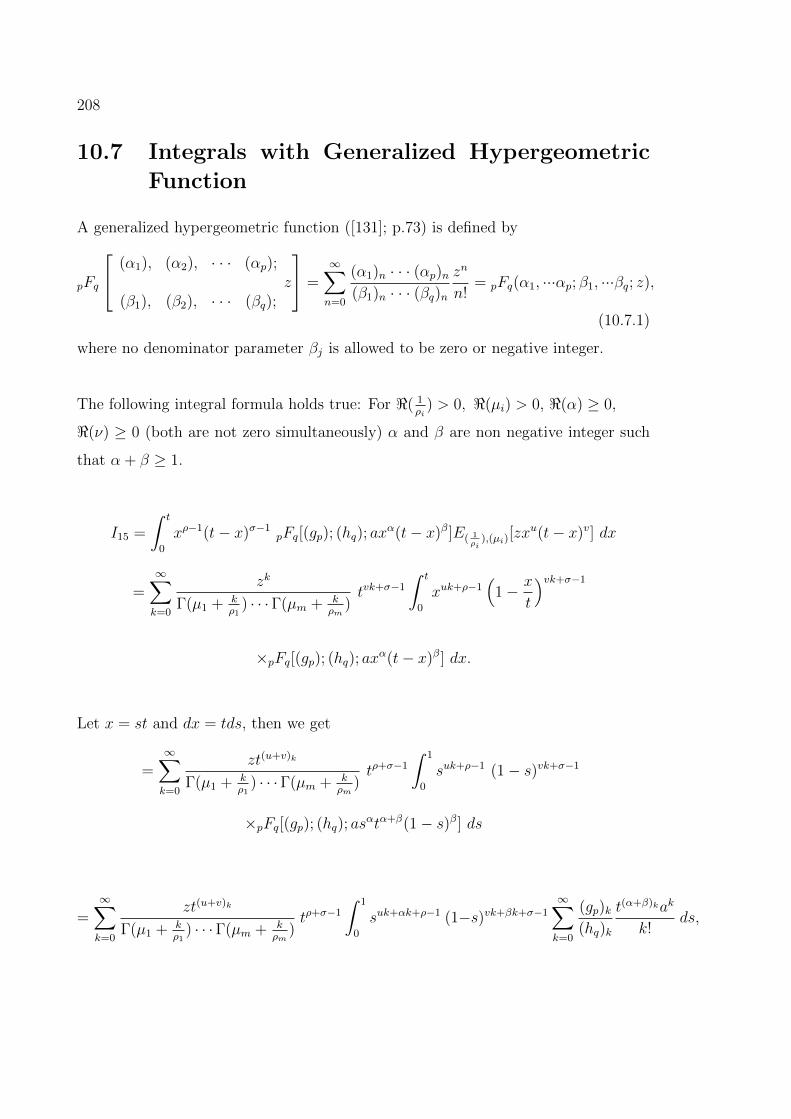
208

10.7 Integrals with Generalized Hypergeometric

Function

A generalized hypergeometric function ([131]; p.73) is defined by

pFq

(α1), (α2), · · · (αp);

(β1), (β2), · · · (βq);z

=∞∑n=0

(α1)n · · · (αp)n(β1)n · · · (βq)n

zn

n!= pFq(α1, ···αp; β1, ···βq; z),

(10.7.1)

where no denominator parameter βj is allowed to be zero or negative integer.

The following integral formula holds true: For <( 1ρi

) > 0, <(µi) > 0, <(α) ≥ 0,

<(ν) ≥ 0 (both are not zero simultaneously) α and β are non negative integer such

that α + β ≥ 1.

I15 =

∫ t

0

xρ−1(t− x)σ−1pFq[(gp); (hq); ax

α(t− x)β]E( 1ρi

),(µi)[zxu(t− x)v] dx

=∞∑k=0

zk

Γ(µ1 + kρ1

) · · ·Γ(µm + kρm

)tvk+σ−1

∫ t

0

xuk+ρ−1(

1− x

t

)vk+σ−1

×pFq[(gp); (hq); axα(t− x)β] dx.

Let x = st and dx = tds, then we get

=∞∑k=0

zt(u+v)k

Γ(µ1 + kρ1

) · · ·Γ(µm + kρm

)tρ+σ−1

∫ 1

0

suk+ρ−1 (1− s)vk+σ−1

×pFq[(gp); (hq); asαtα+β(1− s)β] ds

=∞∑k=0

zt(u+v)k

Γ(µ1 + kρ1

) · · ·Γ(µm + kρm

)tρ+σ−1

∫ 1

0

suk+αk+ρ−1 (1−s)vk+βk+σ−1

∞∑k=0

(gp)k(hq)k

t(α+β)kak

k!ds,

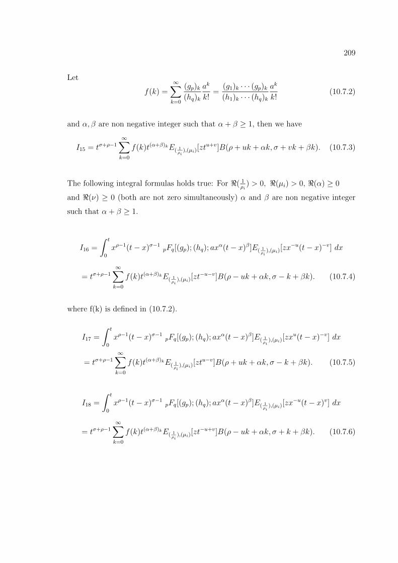
209

Let

f(k) =∞∑k=0

(gp)k(hq)k

ak

k!=

(g1)k · · · (gp)k(h1)k · · · (hq)k

ak

k!(10.7.2)

and α, β are non negative integer such that α + β ≥ 1, then we have

I15 = tσ+ρ−1

∞∑k=0

f(k)t(α+β)kE( 1ρi

),(µi)[ztu+v]B(ρ+ uk + αk, σ + vk + βk). (10.7.3)

The following integral formulas holds true: For <( 1ρi

) > 0, <(µi) > 0, <(α) ≥ 0

and <(ν) ≥ 0 (both are not zero simultaneously) α and β are non negative integer

such that α + β ≥ 1.

I16 =

∫ t

0

xρ−1(t− x)σ−1pFq[(gp); (hq); ax

α(t− x)β]E( 1ρi

),(µi)[zx−u(t− x)−v] dx

= tσ+ρ−1

∞∑k=0

f(k)t(α+β)kE( 1ρi

),(µi)[zt−u−v]B(ρ− uk + αk, σ − k + βk). (10.7.4)

where f(k) is defined in (10.7.2).

I17 =

∫ t

0

xρ−1(t− x)σ−1pFq[(gp); (hq); ax

α(t− x)β]E( 1ρi

),(µi)[zxu(t− x)−v] dx

= tσ+ρ−1

∞∑k=0

f(k)t(α+β)kE( 1ρi

),(µi)[ztu−v]B(ρ+ uk + αk, σ − k + βk). (10.7.5)

I18 =

∫ t

0

xρ−1(t− x)σ−1pFq[(gp); (hq); ax

α(t− x)β]E( 1ρi

),(µi)[zx−u(t− x)v] dx

= tσ+ρ−1

∞∑k=0

f(k)t(α+β)kE( 1ρi

),(µi)[zt−u+v]B(ρ− uk + αk, σ + k + βk). (10.7.6)

Chapter 11

Some Integrals Associated withMultiple (multiindex)Mittag-Leffler Function

11.1 Introduction

A large number of integral formulas involving a variety of special functions of mathe-

matical physics have been developed by a number of authors (see [10], [22], [24], [30],

[31], [151]). Various method available for obtaining integrals of multiple hypergeo-

metric functions, the manipulation of integrals representing the functions may often

be employed and this approach is adopted by us in this chapter.

The main object of the present chapter is to obtain some unified integral formulas

involving multiple (multiindex) Mittag-Leffler function into a series of generalized

Wright hypergeometric function. Some integrals which are used to obtain our main

results are included in section 11.2. Section 11.3 gives integral formulas involving

multiple (multiindex) Mittag-Leffler function and some special cases of these result

are given in section 11.4. Section 11.5 gives another integral formulas involving

multiple (multiindex) Mittag-Leffler function and some special cases of these results

are given in section 11.6.

210

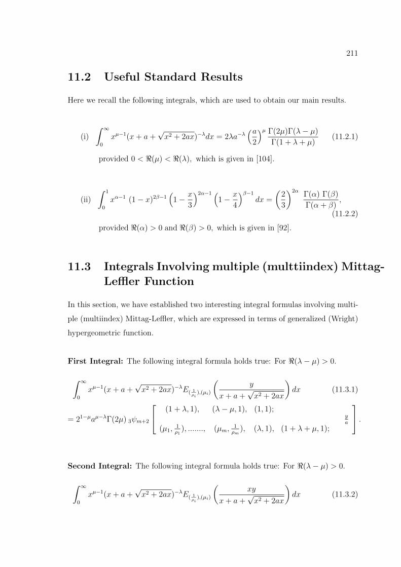
211

11.2 Useful Standard Results

Here we recall the following integrals, which are used to obtain our main results.

(i)

∫ ∞0

xµ−1(x+ a+√x2 + 2ax)−λdx = 2λa−λ

(a2

)µ Γ(2µ)Γ(λ− µ)

Γ(1 + λ+ µ)(11.2.1)

provided 0 < <(µ) < <(λ), which is given in [104].

(ii)

∫ 1

0

xα−1 (1− x)2β−1(

1− x

3

)2α−1 (1− x

4

)β−1

dx =

(2

3

)2αΓ(α) Γ(β)

Γ(α + β),

(11.2.2)

provided <(α) > 0 and <(β) > 0, which is given in [92].

11.3 Integrals Involving multiple (multtiindex) Mittag-

Leffler Function

In this section, we have established two interesting integral formulas involving multi-

ple (multiindex) Mittag-Leffler, which are expressed in terms of generalized (Wright)

hypergeometric function.

First Integral: The following integral formula holds true: For <(λ− µ) > 0.

∫ ∞0

xµ−1(x+ a+√x2 + 2ax)−λE( 1

ρi),(µi)

(y

x+ a+√x2 + 2ax

)dx (11.3.1)

= 21−µaµ−λΓ(2µ) 3ψm+2

(1 + λ, 1), (λ− µ, 1), (1, 1);ya

(µ1,1ρ1

), ......., (µm,1ρm

), (λ, 1), (1 + λ+ µ, 1);

.

Second Integral: The following integral formula holds true: For <(λ− µ) > 0.

∫ ∞0

xµ−1(x+ a+√x2 + 2ax)−λE( 1

ρi),(µi)

(xy

x+ a+√x2 + 2ax

)dx (11.3.2)

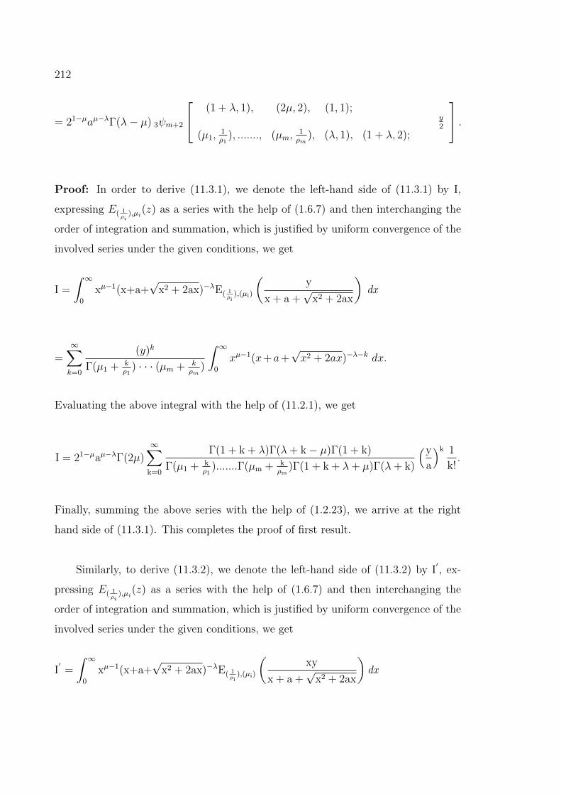
212

= 21−µaµ−λΓ(λ− µ) 3ψm+2

(1 + λ, 1), (2µ, 2), (1, 1);y2

(µ1,1ρ1

), ......., (µm,1ρm

), (λ, 1), (1 + λ, 2);

.

Proof: In order to derive (11.3.1), we denote the left-hand side of (11.3.1) by I,

expressing E( 1ρi

),µi(z) as a series with the help of (1.6.7) and then interchanging the

order of integration and summation, which is justified by uniform convergence of the

involved series under the given conditions, we get

I =

∫ ∞0

xµ−1(x+a+√

x2 + 2ax)−λE( 1ρi

),(µi)

(y

x + a +√

x2 + 2ax

)dx

=∞∑k=0

(y)k

Γ(µ1 + kρ1

) · · · (µm + kρm

)

∫ ∞0

xµ−1(x+a+√x2 + 2ax)−λ−k dx.

Evaluating the above integral with the help of (11.2.1), we get

I = 21−µaµ−λΓ(2µ)∞∑

k=0

Γ(1 + k + λ)Γ(λ+ k− µ)Γ(1 + k)

Γ(µ1 + kρ1

).......Γ(µm + kρm

)Γ(1 + k + λ+ µ)Γ(λ+ k)

(y

a

)k 1

k!.

Finally, summing the above series with the help of (1.2.23), we arrive at the right

hand side of (11.3.1). This completes the proof of first result.

Similarly, to derive (11.3.2), we denote the left-hand side of (11.3.2) by I′, ex-

pressing E( 1ρi

),µi(z) as a series with the help of (1.6.7) and then interchanging the

order of integration and summation, which is justified by uniform convergence of the

involved series under the given conditions, we get

I′=

∫ ∞0

xµ−1(x+a+√

x2 + 2ax)−λE( 1ρi

),(µi)

(xy

x + a +√

x2 + 2ax

)dx

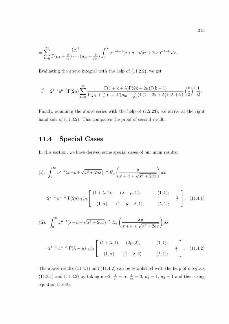
213

=∞∑k=0

(y)k

Γ(µ1 + kρ1

) · · · (µm + kρm

)

∫ ∞0

xµ+k−1(x+a+√x2 + 2ax)−λ−k dx.

Evaluating the above integral with the help of (11.2.2), we get

I′= 21−µaµ−λΓ(2µ)

∞∑k=0

Γ(1 + k + λ)Γ(2k + 2µ)Γ(k + 1)

Γ(µ1 + kρ1

).......Γ(µm + kρm

)Γ(1 + 2k + λ)Γ(λ+ k)

(y

2

)k 1

k!.

Finally, summing the above series with the help of (1.2.23), we arrive at the right

hand side of (11.3.2). This completes the proof of second result.

11.4 Special Cases

In this section, we have derived some special cases of our main results:

(i).

∫ ∞0

xµ−1(x+a+√x2 + 2ax)−λ Eα

(y

x+ a+√x2 + 2ax

)dx

= 21−µ aµ−λ Γ(2µ) 3ψ3

(1 + λ, 1), (λ− µ, 1), (1, 1);ya

(1, α), (1 + µ+ λ, 1), (λ, 1);

. (11.4.1)

(ii).

∫ ∞0

xµ−1(x+a+√x2 + 2ax)−λ Eα

(xy

x+ a+√x2 + 2ax

)dx

= 21−µ aµ−λ Γ(λ− µ) 3ψ3

(1 + λ, 1), (2µ, 2), (1, 1);y2

(1, α), (1 + λ, 2), (λ, 1);

. (11.4.2)

The above results (11.4.1) and (11.4.2) can be established with the help of integrals

(11.3.1) and (11.3.2) by taking m=2, 1ρ1

= α, 1ρ2

= 0, µ1 = 1, µ2 = 1 and then using

equation (1.6.8).

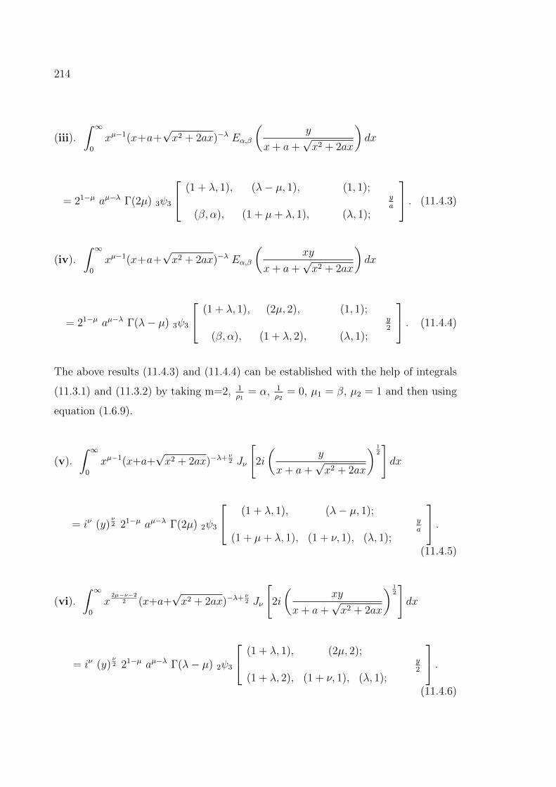
214

(iii).

∫ ∞0

xµ−1(x+a+√x2 + 2ax)−λ Eα,β

(y

x+ a+√x2 + 2ax

)dx

= 21−µ aµ−λ Γ(2µ) 3ψ3

(1 + λ, 1), (λ− µ, 1), (1, 1);ya

(β, α), (1 + µ+ λ, 1), (λ, 1);

. (11.4.3)

(iv).

∫ ∞0

xµ−1(x+a+√x2 + 2ax)−λ Eα,β

(xy

x+ a+√x2 + 2ax

)dx

= 21−µ aµ−λ Γ(λ− µ) 3ψ3

(1 + λ, 1), (2µ, 2), (1, 1);y2

(β, α), (1 + λ, 2), (λ, 1);

. (11.4.4)

The above results (11.4.3) and (11.4.4) can be established with the help of integrals

(11.3.1) and (11.3.2) by taking m=2, 1ρ1

= α, 1ρ2

= 0, µ1 = β, µ2 = 1 and then using

equation (1.6.9).

(v).

∫ ∞0

xµ−1(x+a+√x2 + 2ax)−λ+ ν

2 Jν

[2i

(y

x+ a+√x2 + 2ax

) 12

]dx

= iν (y)ν2 21−µ aµ−λ Γ(2µ) 2ψ3

(1 + λ, 1), (λ− µ, 1);ya

(1 + µ+ λ, 1), (1 + ν, 1), (λ, 1);

.(11.4.5)

(vi).

∫ ∞0

x2µ−ν−2

2 (x+a+√x2 + 2ax)−λ+ ν

2 Jν

[2i

(xy

x+ a+√x2 + 2ax

) 12

]dx

= iν (y)ν2 21−µ aµ−λ Γ(λ− µ) 2ψ3

(1 + λ, 1), (2µ, 2);y2

(1 + λ, 2), (1 + ν, 1), (λ, 1);

.(11.4.6)

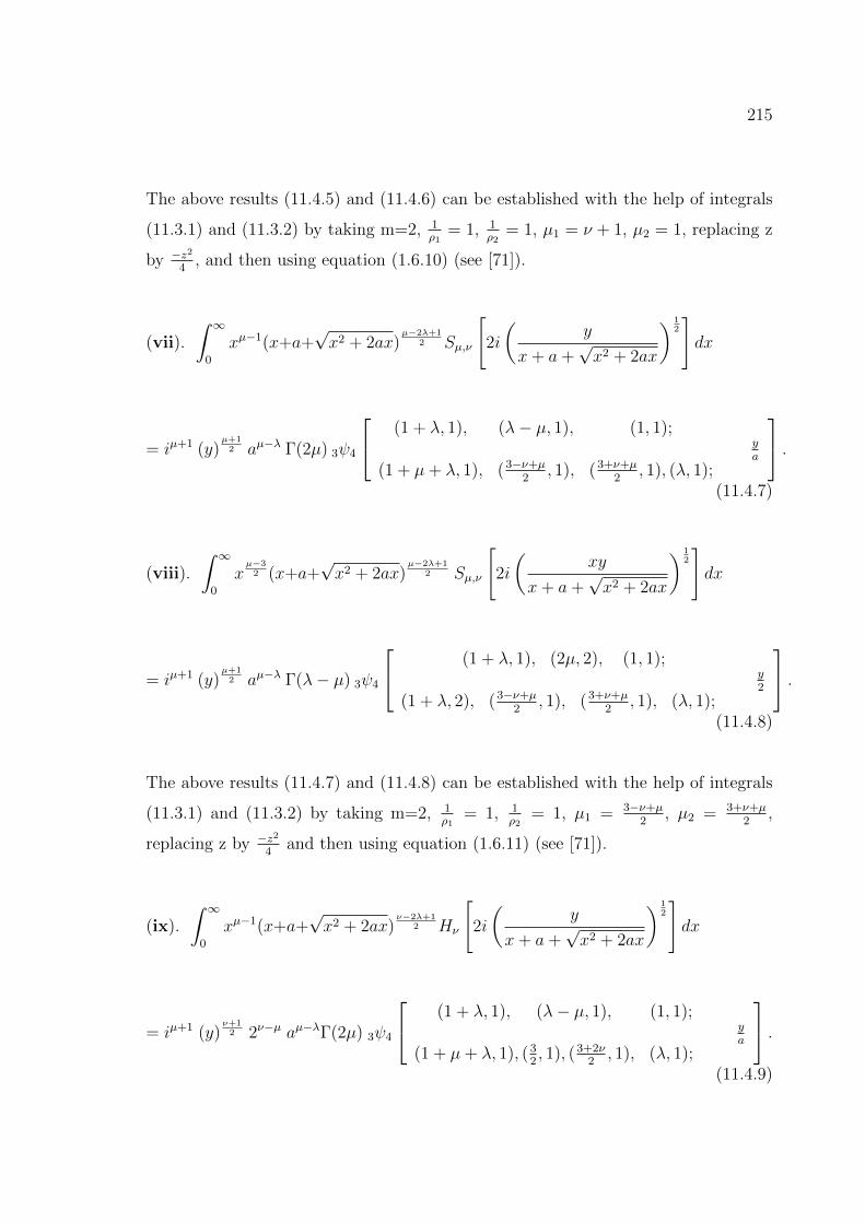
215

The above results (11.4.5) and (11.4.6) can be established with the help of integrals

(11.3.1) and (11.3.2) by taking m=2, 1ρ1

= 1, 1ρ2

= 1, µ1 = ν + 1, µ2 = 1, replacing z

by −z2

4, and then using equation (1.6.10) (see [71]).

(vii).

∫ ∞0

xµ−1(x+a+√x2 + 2ax)

µ−2λ+12 Sµ,ν

[2i

(y

x+ a+√x2 + 2ax

) 12

]dx

= iµ+1 (y)µ+12 aµ−λ Γ(2µ) 3ψ4

(1 + λ, 1), (λ− µ, 1), (1, 1);ya

(1 + µ+ λ, 1), (3−ν+µ2

, 1), (3+ν+µ2

, 1), (λ, 1);

.(11.4.7)

(viii).

∫ ∞0

xµ−32 (x+a+

√x2 + 2ax)

µ−2λ+12 Sµ,ν

[2i

(xy

x+ a+√x2 + 2ax

) 12

]dx

= iµ+1 (y)µ+12 aµ−λ Γ(λ− µ) 3ψ4

(1 + λ, 1), (2µ, 2), (1, 1);y2

(1 + λ, 2), (3−ν+µ2

, 1), (3+ν+µ2

, 1), (λ, 1);

.(11.4.8)

The above results (11.4.7) and (11.4.8) can be established with the help of integrals

(11.3.1) and (11.3.2) by taking m=2, 1ρ1

= 1, 1ρ2

= 1, µ1 = 3−ν+µ2

, µ2 = 3+ν+µ2

,

replacing z by −z2

4and then using equation (1.6.11) (see [71]).

(ix).

∫ ∞0

xµ−1(x+a+√x2 + 2ax)

ν−2λ+12 Hν

[2i

(y

x+ a+√x2 + 2ax

) 12

]dx

= iµ+1 (y)ν+12 2ν−µ aµ−λΓ(2µ) 3ψ4

(1 + λ, 1), (λ− µ, 1), (1, 1);ya

(1 + µ+ λ, 1), (32, 1), (3+2ν

2, 1), (λ, 1);

.(11.4.9)

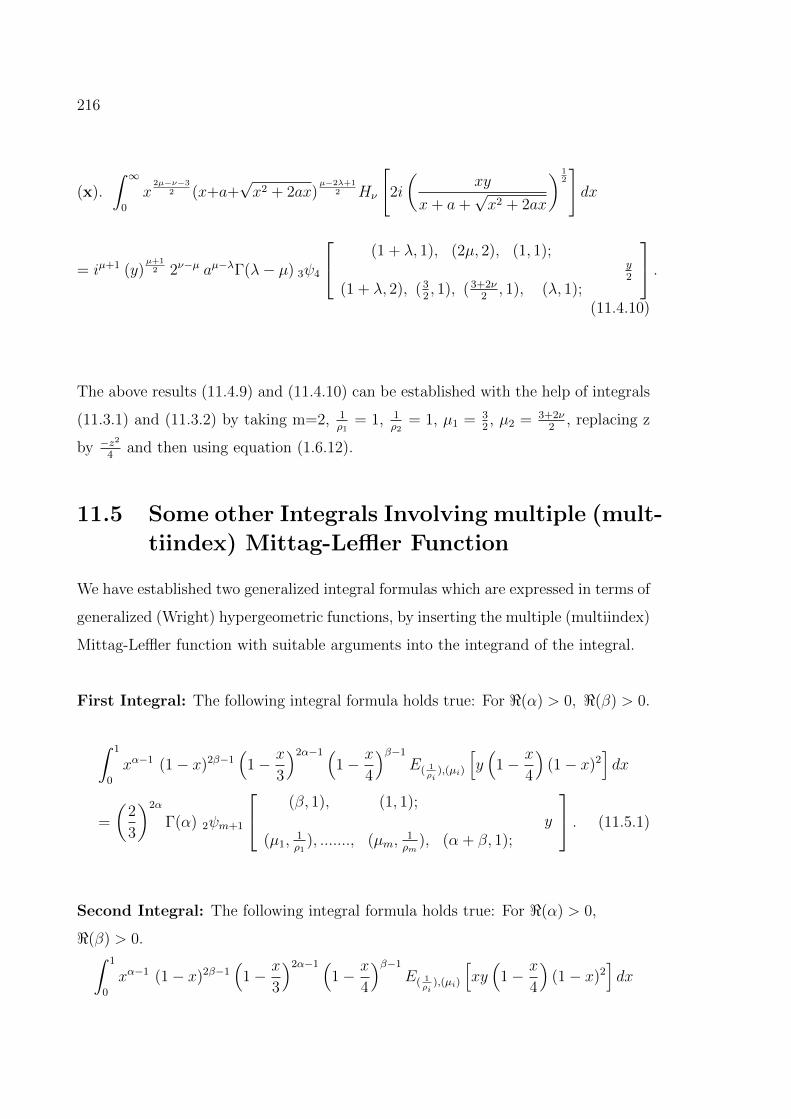
216

(x).

∫ ∞0

x2µ−ν−3

2 (x+a+√x2 + 2ax)

µ−2λ+12 Hν

[2i

(xy

x+ a+√x2 + 2ax

) 12

]dx

= iµ+1 (y)µ+12 2ν−µ aµ−λΓ(λ− µ) 3ψ4

(1 + λ, 1), (2µ, 2), (1, 1);y2

(1 + λ, 2), (32, 1), (3+2ν

2, 1), (λ, 1);

.(11.4.10)

The above results (11.4.9) and (11.4.10) can be established with the help of integrals

(11.3.1) and (11.3.2) by taking m=2, 1ρ1

= 1, 1ρ2

= 1, µ1 = 32, µ2 = 3+2ν

2, replacing z

by −z2

4and then using equation (1.6.12).

11.5 Some other Integrals Involving multiple (mult-

tiindex) Mittag-Leffler Function

We have established two generalized integral formulas which are expressed in terms of

generalized (Wright) hypergeometric functions, by inserting the multiple (multiindex)

Mittag-Leffler function with suitable arguments into the integrand of the integral.

First Integral: The following integral formula holds true: For <(α) > 0, <(β) > 0.

∫ 1

0

xα−1 (1− x)2β−1(

1− x

3

)2α−1 (1− x

4

)β−1

E( 1ρi

),(µi)

[y(

1− x

4

)(1− x)2

]dx

=

(2

3

)2α

Γ(α) 2ψm+1

(β, 1), (1, 1);y

(µ1,1ρ1

), ......., (µm,1ρm

), (α + β, 1);

. (11.5.1)

Second Integral: The following integral formula holds true: For <(α) > 0,

<(β) > 0.∫ 1

0

xα−1 (1− x)2β−1(

1− x

3

)2α−1 (1− x

4

)β−1

E( 1ρi

),(µi)

[xy(

1− x

4

)(1− x)2

]dx

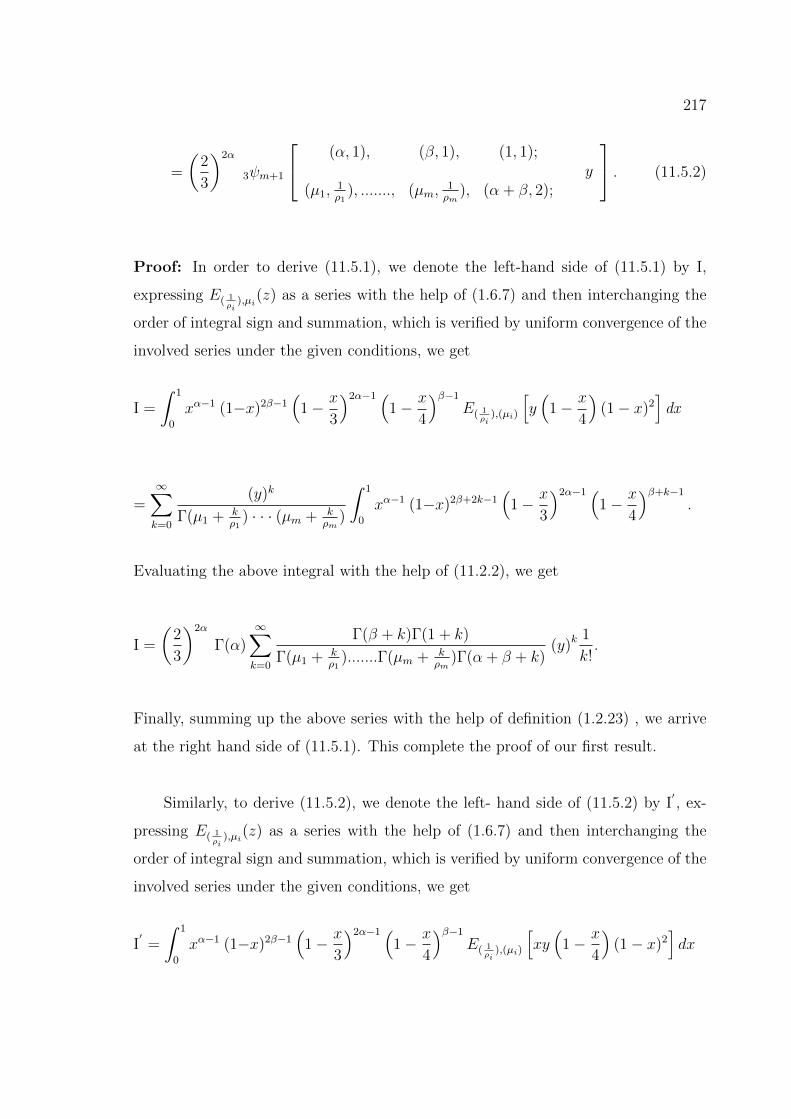
217

=

(2

3

)2α

3ψm+1

(α, 1), (β, 1), (1, 1);y

(µ1,1ρ1

), ......., (µm,1ρm

), (α + β, 2);

. (11.5.2)

Proof: In order to derive (11.5.1), we denote the left-hand side of (11.5.1) by I,

expressing E( 1ρi

),µi(z) as a series with the help of (1.6.7) and then interchanging the

order of integral sign and summation, which is verified by uniform convergence of the

involved series under the given conditions, we get

I =

∫ 1

0

xα−1 (1−x)2β−1(

1− x

3

)2α−1 (1− x

4

)β−1

E( 1ρi

),(µi)

[y(

1− x

4

)(1− x)2

]dx

=∞∑k=0

(y)k

Γ(µ1 + kρ1

) · · · (µm + kρm

)

∫ 1

0

xα−1 (1−x)2β+2k−1(

1− x

3

)2α−1 (1− x

4

)β+k−1

.

Evaluating the above integral with the help of (11.2.2), we get

I =

(2

3

)2α

Γ(α)∞∑k=0

Γ(β + k)Γ(1 + k)

Γ(µ1 + kρ1

).......Γ(µm + kρm

)Γ(α + β + k)(y)k

1

k!.

Finally, summing up the above series with the help of definition (1.2.23) , we arrive

at the right hand side of (11.5.1). This complete the proof of our first result.

Similarly, to derive (11.5.2), we denote the left- hand side of (11.5.2) by I′, ex-

pressing E( 1ρi

),µi(z) as a series with the help of (1.6.7) and then interchanging the

order of integral sign and summation, which is verified by uniform convergence of the

involved series under the given conditions, we get

I′=

∫ 1

0

xα−1 (1−x)2β−1(

1− x

3

)2α−1 (1− x

4

)β−1

E( 1ρi

),(µi)

[xy(

1− x

4

)(1− x)2

]dx

218

=∞∑k=0

(y)k

Γ(µ1 + kρ1

) · · · (µm + kρm

)

∫ 1

0

xα+k−1 (1−x)2β+2k−1(

1− x

3

)2α−1 (1− x

4

)β+k−1

.

Evaluating the above integral with the help of (11.2.2), we get

I′=

(2

3

)2α ∞∑k=0

Γ(α + k)Γ(β + k)Γ(1 + k)

Γ(µ1 + kρ1

).......Γ(µm + kρm

)Γ(α + β + 2k)(y)k

1

k!.

Finally, summing up the above series with the help of definition (1.2.23) , we arrive

at the right hand side of (11.5.2). This complete the proof of our second result.

11.6 Special Cases

In this section, we have derived some special cases of our main results:

(i).

∫ 1

0

xα−1 (1−x)2β−1(

1− x

3

)2α−1 (1− x

4

)β−1

Eα

[y(

1− x

4

)(1− x)2

]dx

=

(2

3

)2α

Γ(α) 2ψ2

(β, 1), (1, 1);y

(α, 1), (α + β, 1);

, (11.6.1)

where <(α) > 0, <(β) > 0.

(ii).

∫ 1

0

xα−1 (1−x)2β−1(

1− x

3

)2α−1 (1− x

4

)β−1

Eα

[xy(

1− x

4

)(1− x)2

]dx

=

(2

3

)2α

3ψ2

(α, 1), (β, 1), (1, 1);y

(α, 1), (α + β, 2);

, (11.6.2)

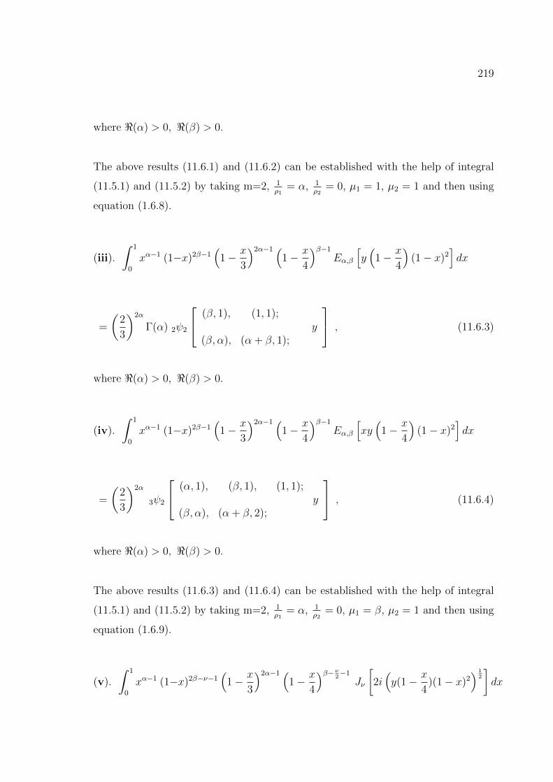
219

where <(α) > 0, <(β) > 0.

The above results (11.6.1) and (11.6.2) can be established with the help of integral

(11.5.1) and (11.5.2) by taking m=2, 1ρ1

= α, 1ρ2

= 0, µ1 = 1, µ2 = 1 and then using

equation (1.6.8).

(iii).

∫ 1

0

xα−1 (1−x)2β−1(

1− x

3

)2α−1 (1− x

4

)β−1

Eα,β

[y(

1− x

4

)(1− x)2

]dx

=

(2

3

)2α

Γ(α) 2ψ2

(β, 1), (1, 1);y

(β, α), (α + β, 1);

, (11.6.3)

where <(α) > 0, <(β) > 0.

(iv).

∫ 1

0

xα−1 (1−x)2β−1(

1− x

3

)2α−1 (1− x

4

)β−1

Eα,β

[xy(

1− x

4

)(1− x)2

]dx

=

(2

3

)2α

3ψ2

(α, 1), (β, 1), (1, 1);y

(β, α), (α + β, 2);

, (11.6.4)

where <(α) > 0, <(β) > 0.

The above results (11.6.3) and (11.6.4) can be established with the help of integral

(11.5.1) and (11.5.2) by taking m=2, 1ρ1

= α, 1ρ2

= 0, µ1 = β, µ2 = 1 and then using

equation (1.6.9).

(v).

∫ 1

0

xα−1 (1−x)2β−ν−1(

1− x

3

)2α−1 (1− x

4

)β− ν2−1

Jν

[2i(y(1− x

4)(1− x)2

) 12

]dx

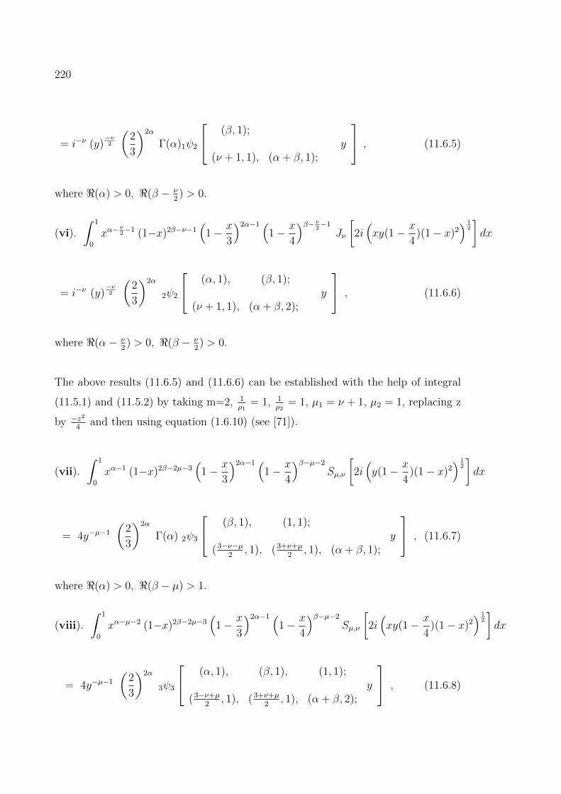
220

= i−ν (y)−ν2

(2

3

)2α

Γ(α)1ψ2

(β, 1);y

(ν + 1, 1), (α + β, 1);

, (11.6.5)

where <(α) > 0, <(β − ν2) > 0.

(vi).

∫ 1

0

xα−ν2−1 (1−x)2β−ν−1

(1− x

3

)2α−1 (1− x

4

)β− ν2−1

Jν

[2i(xy(1− x

4)(1− x)2

) 12

]dx

= i−ν (y)−ν2

(2

3

)2α

2ψ2

(α, 1), (β, 1);y

(ν + 1, 1), (α + β, 2);

, (11.6.6)

where <(α− ν2) > 0, <(β − ν

2) > 0.

The above results (11.6.5) and (11.6.6) can be established with the help of integral

(11.5.1) and (11.5.2) by taking m=2, 1ρ1

= 1, 1ρ2

= 1, µ1 = ν + 1, µ2 = 1, replacing z

by −z2

4and then using equation (1.6.10) (see [71]).

(vii).

∫ 1

0

xα−1 (1−x)2β−2µ−3(

1− x

3

)2α−1 (1− x

4

)β−µ−2

Sµ,ν

[2i(y(1− x

4)(1− x)2

) 12

]dx

= 4y−µ−1

(2

3

)2α

Γ(α) 2ψ3

(β, 1), (1, 1);y

(3−ν−µ2

, 1), (3+ν+µ2

, 1), (α + β, 1);

, (11.6.7)

where <(α) > 0, <(β − µ) > 1.

(viii).

∫ 1

0

xα−µ−2 (1−x)2β−2µ−3(

1− x

3

)2α−1 (1− x

4

)β−µ−2

Sµ,ν

[2i(xy(1− x

4)(1− x)2

) 12

]dx

= 4y−µ−1

(2

3

)2α

3ψ3

(α, 1), (β, 1), (1, 1);y

(3−ν+µ2

, 1), (3+ν+µ2

, 1), (α + β, 2);

, (11.6.8)

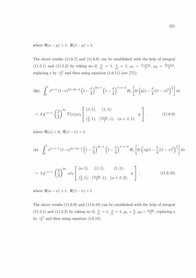
221

where <(α− µ) > 1, <(β − µ) > 1.

The above results (11.6.7) and (11.6.8) can be established with the help of integral

(11.5.1) and (11.5.2) by taking m=2, 1ρ1

= 1, 1ρ2

= 1, µ1 = 3−ν+µ2

, µ2 = 3+ν+µ2

,

replacing z by −z2

4and then using equation (1.6.11) (see [71]).

(ix).

∫ 1

0

xα−1 (1−x)2β−2ν−3(

1− x

3

)2α−1 (1− x

4

)β−ν−2

Hν

[2i(y(1− x

4)(1− x)2

) 12

]dx

= 4 y−ν−1

(2

3

)2α

Γ(α)2ψ3

(β, 1), (1, 1);y

(32, 1), (3+2ν

2, 1), (α + β, 1);

, (11.6.9)

where <(α) > 0, <(β − ν) > 1.

(x).

∫ 1

0

xα−ν−2 (1−x)2β−2ν−3(

1− x

3

)2α−1 (1− x

4

)β−ν−2

Hν

[2i(xy(1− x

4)(1− x)2

) 12

]dx

= 4 y−ν−1

(2

3

)2α

3ψ3

(α, 1), (β, 1), (1, 1);y

(32, 1), (3+2ν

2, 1), (α + β, 2);

, (11.6.10)

where <(α− ν) > 1, <(β − ν) > 1.

The above results (11.6.9) and (11.6.10) can be established with the help of integral

(11.5.1) and (11.5.2) by taking m=2, 1ρ1

= 1, 1ρ2

= 1, µ1 = 32, µ2 = 3+2ν

2, replacing z

by −z2

4and then using equation (1.6.12).

Bibliography

[1] Agarwal, P.; On a new unified integral involving hypergeometric functions, Ad-

vances in Computational Mathematics and its Applications, Vol.2, No.1 (2012),

239-242.

[2] Agarwal, P.; New unified integrals involving a Srivastava polynomials and H-

function, Journal of Fractional Calculus and Applications, Vol.3, No.3 (2012),

1-7.

[3] Agarwal, P.; A study of New Trends and Analysis of Special Function, Lambert

Academic Publishing, (2013).

[4] Ali, S.; On some new unified integrals, Advances in Computational Mathematics

and its Applications, Vol. 1 No.3 (2012), 151-153.

[5] Andrew, L.C., Special functions for engineering and applied mathematicians,

The McMillan Company, New York, (1985).

[6] Apostol, T.M.; On the Lerch zeta function, Pacific J.Math. 1 (1951), 161-167.

[7] Appell, P.; Sur les series hypergeometriques de deux variable, et sur des equations

differentielles Lineaires aux derivee partielles, C.R. Acad Sci., paris, 90 (1880),

296-298.

[8] Appell, P. and Kampe′ de Fe′riet , J., Fonctions hypergeometriques et hyper-

spheriques, Polynomes d’Hermite Gauthier-Villar,Paris, (1926).

222

223

[9] Abramowitz, M. and Stegun, I.A.; Handbook of mathematical functions with

formulas graphs and mathematical tables, National Bureau of Standards, Wash-

ington, DC, 1964.

[10] Agarwal, P., Jain, S., Agarwal, S. and Nagpal, M.; On a new class of integrals in-

volving Bessel functions of the first kind, Communication in Numerical Analysis,

2014 (2014), 1-7.

[11] Bailey, W.N., Generalized hypergeometric series, Cambridge University Press,

London (1935).

[12] Bailey, W.N., On the product of two Legendre polynomials with different argu-

ments, Proc. London Math. Soc. (2), 41 (1936), 215-220.

[13] Bailey, W.N., On the product of two Laguerre polynomials, Quart. J. Math. Vol.

X (1939), 60-66.

[14] Bell, E.T.; Exponential polynomials, Ann. of Math. 35 (1934), 258-277.

[15] Brychkov, Y. A.; Handbook of Special Functions: Derivatives, Integrals, Series

and Other Formulas, CRC Press, Boca Raton (2008).

[16] Brychkov, Y. A., On multiple sums of special functions, Integral Trans. Spec.

Func., 21 (12) (2010), 877-884.

[17] Bayad, A. and Hamahata, Y.; Poly-Euler polynomials and Arakawa-Kaneko type

zeta functions, Preprint.

[18] Belafhal, A. and Hennani, S.; A note on integrals used in laser field involving

the product of Bessel functions, Phys. Chem. News 61 (2011) 59-62.

[19] Carlson, B.C.; Special function of Applied Mathematics, Academic Press, New

York, ( 1977).

[20] Chun-Fang Li; Integral transformation solution of free-space cylindrical vector

beams and pridiction of modified-Bessel-Gaussian vector beams, (2008).

224

[21] Comlet, L.; The art of finite and infinite expansions, (Translated from french by

J. W. Nilenhuys), Reidel, Dordrecht, 1974.

[22] Choi, J. and Agarwal, P.; Certain unified integrals associated with Bessel func-

tions, Boundary Value Problems, 2013 (95) (2013), 1-9.

[23] Choi, J. and Agarwal, P.; Certain integral transform and fractional integral for-

mulas for the generalized Gauss hypergeometric functions, Abstract and Applied

Analysis, Vol. 2014 (2014), 1-7.

[24] Choi, J. and Agarwal, P.;, Certain unified integrals involving a product of Bessel

functions of first kind, Honam Mathematical J. (4) 35 (2013), 667-677.

[25] Choudhary, C. and Chaudhary, P.; Integrals associated with generalized K-

Mittag-Leffler function, N.T.M.SCI., 3, No. 3, (2015) 103-115.

[26] Choi, J., Ghayasuddin. M. and Khan, N.U.; Generalized extended Whittaker

function and its properties, App. Math. Sci., 9, (2015), 6529-6541.

[27] Cangul, I.N., Kurt, V., Ozden, H., Simsek, Y.; On the higher order w-q-Genocchi

numbers, Adv. Stud. Contemp. Math. 19 (1) (2009), 39-57.

[28] Chaudhry, M.A., Qadir, A., Rafique, M. and Zubair, S.M.; Extension of Euler’s

beta function, J. Comput. Appl. Math., 78 (1997), no.1, 19-32.

[29] Chaudhry, M.A., Qadir, A., Srivastava, H.M. and Paris, R.B.; Extended hyper-

geometric and confluent hypergeometric functions, Appl. Math. Comput., 159

(2004), no.2, 589-602.

[30] Choi, J., Agarwal, P., Mathur, S. and Purohit, S.D.; Certain new integral for-

mulas involving the generalized Bessel functions, Bull. Korean Math. Soc., 51

(2014), no.4, 995-1003.

[31] Choi, J., Hasnove, A., Srivastava, H.M. and Turaev, M.; Integral representations

for Srivastava’s triple hypergeometric functions, Taiwanese J. Math. 15 (2011),

no. 6, 2751-2762.

225

[32] Dilcher, K.; Asymptotic behavior of Bernoulli, Euler and generalized Bernoulli

polynomials, J.Approx.Theory 49 (1987), 321-330.

[33] Dattoli, G. and Torre, A.; Operational methods and two variable Laguerre poly-

nomials, Atti Acadmia di Torino, 132 (1998), 1-7.

[34] Dere, R. and Simsek, Y.; Genocchi polynomials associated with the Umbral

algebra, Appl. Math. Comput. 218 (3) (2011), 756-761.

[35] Ditkin, V.A. and Prudnikov, A.P.; Integral transform and operational calculus,

Moscow, Transpergaman Press, Oxford, (1965).

[36] Dattoli, G., Lorenzutta, S. and Cesarano, C.; Finite sums and generalized forms

of Bernoulli polynomials Rendiconti di Mathematica, 19 (1999), 385-391.

[37] Edward, J.; A Treatise on the integral calculas, Vol. II, Chelsea Publishing

Company, New York, (1922).

[38] Exton, H.; A new generating function for the associated Laguerre polynomials

and resulting expansions, Jnan ˜abha, 13 (1983), 147-149.

[39] Exton, H.; Multiple hypergeometric functions and applications, Halsted Press

(Ellis Horwood Ltd., Chichester, U.K), ( 1976).

[40] Erdelyi, A. et. al.; On some expansions in Laguerre polynomials, J. London

Math. Soc. 13 (1938), 154-156.

[41] Erdelyi, A. et. al.; Transformation of hypergeometric functions of two variables,

Proc. Roy . Soc.Edinburg Sect. A, 62 (1948), 378-385.

[42] Erdelyi, A. et. al.; Higher transcendental functions, Vol. I, McGraw-Hill Book

Co. In., New York, Toronto and London, (1953).

[43] Erdelyi, A. et. al.; Higher transcendental functions, Vol. II, McGraw-Hill Book

Co. In., New York, Toronto and London, (1953).

226

[44] Erdelyi, A. et. al.; Higher transcendental functions, Vol. III, McGraw-Hill Book

Co. In., New York, Toronto and London, (1955).

[45] Erdelyi, A. et. al.; Tables of integral transforms, Vol. I, McGraw-Hill Book Co.

In., New York, Toronto, London, (1954).

[46] Erdelyi, A. et al.; Tables of integral transforms, Vol. II, McGraw-Hill Book Co.

In., New York, Toronto, London, (1954).

[47] Feldheim, E.; Relation entre les polynomes de Jacobi, Laguerre et Hermite. Acta

Math., 74 (1941), 117-138.

[48] Fox, C.; The asymptotic expansion of generalized hypergeometric functions,

Proc. Lond. Math. Soc., 27 (1928), 389-400.

[49] Fried, B.D. and Conte, S.D.; The plasma dispersion function, Academic press,

New York, (1961).

[50] Garg, M. and Jain, K.; Some new representations of Voigt function, Proc. of the

7th Int. Conf. SSFA 7 (2006), 89-100.

[51] Garg, M. and Mittal, S.; On a new unified integral, Proc. Indian Acad. Sci.

Math. Sci. 114(2) (2003), 99-101.

[52] Goyal, S.P. and Mukherjee, R.; Generalizations of the Voigt functions through

generalized Lauricella function, Ganita Sandesh, 13(1) (1999), 31-41.

[53] Gradshteyn, I.S. and Rhyzik, I.M.; Table of Integrals, Series and Products, 5th

ed. Academic Press, New York (1994).

[54] Gupta, K. and Gupta, A.; On the study of unified representations of the gener-

alized Voigt functions, Palestine Journal of Mathematics, 2(1) (2013), 32-37.

[55] Gupta, K.C., Goyal, S.P. and Mukherjee, R.; Some results on generalized Viogt

functions, ANZIAM J., 44 (2002), 299-303.

227

[56] Hansen, E.R.; A table of series and products, Printice Hall, Englewood Cliffs,

NJ, (1975).

[57] Humbert, P.; The Confluent hypergeometric function of two variables, Proc.

Roy.Soc. Edinbergh., 41 (1920), 73-96.

[58] Hamahata, Y., Masubuch, H.; Special Multi-Poly- Bernoulli numbers, Journal

of Integer sequences, 10 (2007), 1-6.

[59] Hamahata, Y., Masubuchi, H.; Recurrence formulae for Multi-poly-Bernoulli

numbers, Elec. J.Comb.Num.Theo. 7 (2007), A-46.

[60] He. Y, Araci. S, Srivastava, H.M., Acikgoz, M.; Some new identities for the

Apostol-Bernoulli polynomials and Apostol- Genocchi polynomials, Appl.Math.

and Comput. 262 (2015), 31-41.

[61] Jolany, H., Corcino, R.B.; Explicit formula for generalization of Poly-Bernoulli

numbers and polynomials with a,b,c parameters, Journal of Classical Analysis,

6 (2015), 119-135.

[62] Jolany, H and Corcino, R.B.; More properties on Multi-Euler polynomials,

arXiv;1401. 627 IvI [math NT] 24 Jan 2014.

[63] Jolany, H., Darafsheh, M.R., Alikelaye,R.E.; Generalizations of Poly-Bernoulli

Numbers and Polynomials, Int. J. Math. Comb. 2 (2010), A 07-14.

[64] Jolany, H., Aliabadi, M., Corcino, R. B. and Darafsheh, M.R.; A Note on

Multi Poly-Euler Numbers and Bernoulli Polynomials, General Mathematics,

20 (2012), 122-134.

[65] Kaneko, M.; Poly-Bernoulli numbers, J.de Theorie de Nombres 9 (1997), 221-

228.

[66] Khan, N.U.; A new class of generating functions associated with the product of

Laguerre polynomials, South East Asian J. Math. and Math. Sc. vol. 3, No.2

(2005), 65-70.

228

[67] Khan, W.A.; A new class of Hermite poly-Genocchi polynomials, Journal of

Analysis and Number Theory, 4, No.1,(2016), 1-8.

[68] Khan, W.A.; Some properties of the generalized Apostol type Hermite-based

polynomials, Kyungpook Math. J. 55 (2015), 597-614.

[69] Khan, W.A.; A note on Hermite-Based poly-Euler and Multi poly-Euler poly-

nomials, Palestine Journal of Mathematics, 5 (1), (2016), 17-26.

[70] Kim, T.; Some identities for the Bernoulli, the Euler and the Genocchi numbers

and polynomials, Adv. Stud. Contemp. Math. 20 (1) (2010), 23-28.

[71] Kiryakova, V.S.; Multiple (multiindex) Mittag-Leffler functions and relations to

generalized fractional calculus, J. Comput. Appl. Math., 118 (2000) 241-259.

[72] Klusch, D., Astrophysical Spectroscopy and neutron reactions, Integral trans-

forms and Voigt functions, Astrophys. Space Sci., 175 (1991), 229-240.

[73] Kummar, E.E.; Uber die hypergeometriche Reihe F (a; b;x), J. Reine Angew.

Math., 15 (1836), 39-83 and 127-172.

[74] Khan, N.U. and Ghayasuddin, M.; A note on generalized extended Whittaker

Function, Honam Math. J., (2016) (Accepted).

[75] Khan, N.U. and Ghayasuddin, M.; Study of the unified integral associated with

Bessel-Maitland function. Pure and Applied Mathematics Letters Vol. 2016

(2016) 15-19.

[76] Khan, N.U. and Ghayasuddin, M.; Certain new representations of the generalized

Voigt functions, under communication (2015).

[77] Khan, N.U. and Ghayasuddin, M.; Some unified integral associated with whit-

taker functions, Journal of Mathematical Analysis (Accepted).

[78] Khan, N.U. and Ghayasuddin, M.; A new class of integral formulas associated

with generalized Bessel functions, (Communicated).

229

[79] Khan, N. U. and Kashmin. T.; Integral Transforms involving Bessel’s Function,

Communicated to Honam Mathematical Journal.

[80] Khan, N.U., Usman, T. and Ghayasuddin, M.; A new class of unified integral

formulas associated with Whittaker functions, New Trends in Mathematical Sci-

ences, Vol. 4, No. 1 (2016), 160-167.

[81] Khan, N.U., Kamarujjama, M. and Ghayasuddin, M.; A generalization of Voigt

function involving generalized Whittaker and Bessel functions, Palestine Journal

of Mathematics, 4(2)(2015), 313-318.

[82] Karimi, E., Piccirillo, B., Marrucci, L. and Santamato, E.; Improved focus-

ing with hypergeometric-guassian type-II optical modes, Optics Express, 16N25

(2008) 21069.

[83] Kim, T., Rim, S.H., Simsek, Y. and Kim, D.; On the analogous of Bernoulli and

Euler numbers related identities and zeta and L-functions, J. Korean. Math. Soc.

45 (2008), 435-453.

[84] Khan, S., Pathan, M.A., Hassan, Nader Ali Makhboul , Yasmin, G.; Implicit

summation formula for Hermite and related polynomials, J.Math.Anal.Appl.

344 (2008), 408-416.

[85] Lauricella, G.; Sulle funzioni ipergeometriche a piu variabili, Rend. Circ. Mat.

Palermo, 7, (1893), 111-158.

[86] Lebedev, N.N.; Special functions and their application, New Jersey, (1965).

[87] Luke, Y,; The special functions and their approximations, Vols. 1-2, (1969).

[88] Luo, Q.M.; The multiplication formulas for the Apostol-Bernoulli and Apostol-

Euler polynomials of higher order, Integral Trans. Spec. Funct. 20 (2009), 377-

391.

[89] Luo, Q.M.; Apostol Euler polynomials of higher order and gaussian hypergeo-

metric functions, Taiwanese J. Math., 10 (4)(2006), 917-925.

230

[90] Luo, Q.M.; q-extensions for the Apostol-Genocchi polynomials, Gen. Math., 17

(2) (2009), 113-125.

[91] Luo, Q.M.; Extensions for the Genocchi polynomials and its fourier expansions

and integral representations, Osaka J. Math., 48 (2011), 291-310.

[92] Lavoie, J.L. and Trottier, G.; On the sum of certain Appell’s series, Ganita, (1)

20 (1969), 31-32.

[93] Lu, D.Q. and Luo, Q.M.; Some properties of the generalized Apostol type poly-

nomials, Boundary Value Problems, 2013 (2013), 64.

[94] Luo, Q.M. and Srivastava, H.M.; Some generalizations of the Apostol-Bernoulli

and Apostol-Euler polynomials, J. Math. Anal. Appl, 308(1) (2005), 290-302.

[95] Luo, Q.M. and Srivastava, H.M.; Some generalizations of the Apostol Genocchi

poly- nomials and the stirling number of the second kind, Appl. Math. Comput,

217 (2011), 5702-5728.

[96] Luo, Q.M. and Srivastava, H.M. Some relationships between the Apostol-

Bernoulli and Apostol-Euler polynomials, Comput. Math. Appl, 51 (2006), 631-

642.

[97] Lee, D.M., Rathie, A.K. and Parmar, R.K.; Generatization of extended beta

function, hypergeometric and confluent hypergeometric function, Honam Math-

ematical Journal, 33 (2), (2011), 187-206.

[98] Mayer, K.; Uber bestimmte integrale and hypergeometriche funktionen, S-B.

Acad. Wiss. Wien Abt. IIa. Math. Natur. KI., 141 (1932), 227-265.

[99] McBride, E.B.; Obtaining generating function, Springer Verlage, New York Hei-

delberg and Berlin, (1971).

[100] Mittag-Leffler, G.M.; Sur la nouvelle function Eα(x), Comptes Rendus de lA-

cademie des Sciences, Vol. 137 (1903), 554-558.

231

[101] Magnus, F., Oberhettinger, W. and Soni, R.P.; Some formulas and theorem for

the special functions of mathematical physics, Third enlarged edition, Springer-

Verlag, New York, (1966).

[102] Norlund, N.E.; Volessungen uber Dierenzenrechung, Springer 1924.

[103] Nagar, D.K., Vasquez, R.A.M., and Gupta, A.K.; Properties of the Extended

Whittaker Function, Progress in Applied Mathematics, Vol. 6(2013), no. 2, 70-

80.

[104] Oberhettinger, F.; Tables of Mellin Transforms, Springer, New York, (1974).

[105] Ozarslan, M.A.; Hermite-Based unified Apostol-Bernoulli, Euler and Genocchi

polynomials, Advan. Diff. Eqtn. doi:10.1186/1687-1847-213-116, 2013.

[106] Ozarslan, M.A.; Unified Apostol-Bernoulli, Euler and Genocchi polynomials,

Comput. Math. Appl. 6 (2011), 2452-2462.

[107] Ozden, H.; Unification of generating functions of the Bernoulli, Euler and

Genocchi numbers and polynomials, Numerical Anal.and Appl.Math., AIP,Conf.

Proc. 1281 (2010), 1125-1127.

[108] Ozden, H.; Generating function of the unified representation of the Bernoulli,

Euler and Genocchi polynomials of higher order, to appear in Numerical

Anal.and Appl.Math.,AIP,Conf.Proc.(2011).

[109] Ohno, Y. and Sasaki, Y.; On poly-Euler Numbers, Reprint.

[110] Ozden, H., Simsek. Y. and Srivastava, H.M.; A unified presentation of the gen-

erating functions of the generalized Bernoulli, Euler and Genocchi polynomials,

Comput. Math. Appl. 60 (2010), 2779-2287.

[111] Ozergin, E., Ozarslan, M.A., and Altin, A.; Extension of gamma, beta and

hypergeometric functions, J. Comput. Appl. Math. 235(2011), 4601-4610.

232

[112] Pathan, M.A.; On a transformation of a general hypergeometric series of four

variables, Nederl , Akad. Wetensch. Proc Ser . A, 82=Indag Math 41 (1979),

171-175.

[113] Pathan, M.A: On a generalized hypergeometric function of (n+1) variables, J.

National Chiao Tung Univ. 6 (1979), 51-59.

[114] Pathak, R.S.; Certain convergence theorems and asymptotic properties of a

generalization of Lommel and Maitland transform, Proc. U. S. Nat. Acad. Sci.

Sect. A., 36 (1996), 81-86.

[115] Parmar, R.K.; A New Generalization of Gamma, Beta, Hypergeometric

and Confluent Hypergeometric Functions, LE MATEMATICHE, Vol. LXVIII

(2013), 33-52.

[116] Prabhakar, T.R.; A singular integral equation with a generalized Mittag-Leffler

function in the kernel , Yokohama Mathematical Journal, Vol. 19 (1971), 7-15.

[117] Pathan, M.A. and Khan, W.A.; A new class of generalized polynomials associ-

ated with Hermite and Bernoulli polynomials, LE MATEMATICHE, Vol. LXX

(2015), 53-70.

[118] Pathan, M.A. and Khan, W.A.; A new class of generalized Hermite-Bernoulli

polynomials, Georgian Math. J. 19 (2012), 559-573.

[119] Pathan, M.A. and Khan, W.A.; Some implicit summation formulas and sym-

metric identities for the generalized Hermite based- polynomials, Acta Universi-

tatis Apulensis, 39 (2014), 113-136.

[120] Pathan, M.A. and Khan, W.A.; Some implicit summation formulas and sym-

metric identities for the generalized Hermite-Bernoulli polynomials, Mediterr. J.

Math. 12 (2015), 679-695.

[121] Pathan, M.A. and Khan, W.A.; A new class of generalized polynomials

associated with Hermite and Euler polynomials, Mediterr. J. Math. DOI

10.1007/s00009-015-0551-1, Springer Basel (2015).

233

[122] Pathan, M.A. and Khan, W.A.; Some implicit summation formulas and sym-

metric identities for the generalized Hermite-Euler polynomials, East-West

J.Maths. 16 (2014), 92-109.

[123] Pathan M.A. and Khan, W.A.; Some new classes of generalized Hermite-based

Apostol-Euler and Apostol-Genocchi polynomials, Fasciculli.Math. 55 (2015),

158-170.

[124] Pathan, M.A. and Shahwan, M.J.S.; New representation of the Voigt functions,

Demonstratio Math., 39 (2006), 1-4.

[125] Pathan, M.A. and Yasmeen, On partly bilateral and partly unilateral generating

functions, J.Austral. Math. Soc., Ser. B 28 (1986), 240-245.

[126] Pathan, M.A. and Kamarujjama, M.; On certain mixed generating functions,

Journal of Analysis, Forum D’Analystes, 6 (1998), 1-6.

[127] Pathan, M.A., Gupta, K. and Agrawal, V.; Summation formulae involving

Voigt functions and generalized hypergeometric functions, SCIENTIA Series, A

Mathematical Sciences, 19 (2010), 37-44.

[128] Pathan, M.A., Garg, M. and Mittal, S.; On unified presentations of the multi-

variable Voigt functions, East-West J. Math. 8 (2006), No. 1, 49-59.

[129] Prudnikov, A.P. Brychknov, Yu.A. and Marochev, O.I.; Integrals and series Vol-

3; (More special function.) Nauka Moscow, 1986, Translated from the Russian

by G.G.Gould, Gardan and Breach Sience Publishers, New York, Philadelphia.

London, Paris, Montreux, Tokyo, Melbourne, (1990).

[130] Prudnikov, A.P., Brychknov, Yu.A. and Marichev, O.I.; Integrals and series of

elementary functions in (Russian), Nauka, Moscow (1981).

[131] Rainville, E.D.; Special functions, The Macmillan Co. Inc., New York, (1960).

[132] Saran, S.; Hypergeometric functions of three variables, Ganita, 5 (2)(1954),

71-91; Corrigendum Ibid. 7 (1956), 65.

234

[133] Saxena, V.P.; The I-Function , Anamaya publisher, New Delhi, (2008).

[134] Salim, TO.; Some properties relating to the generalized Mittag-Leffler function,

Adv. Appl. Math. Anal. 4, 2130.

[135] Shahabuddin, M.; A set of polynomials, Ranchi Univ. Math. J., 8 (1977), 17-28.

[136] Siegman, A.E.; New Developments in Laser Resonators Proc. SPIE 1224

(1990), 2-12.

[137] Siegman, A.E.; How to (maybe) measure laser beam quality, OSA TOPS 17

(1998), 184-199.

[138] Simsek, Y.; Generating functions of the twisted Bernoulli numbers and polyno-

mials associated with their interpolation functions, Adv. Stud. Contemp. Math.

16 (2008), 251-278.

[139] Slater, L.J.; Confluent hypergeometric functions, Cambridge Univ, Press, New

York, (1960).

[140] Srivastava, H.M.; Some formulas for the Bernoulli and Euler polynomials at

rational arguments, Math. Proc. Cambridge Philos. Soc. 129 (2000),77-84.

[141] Srivastava, H.M.; Generalized Neuman expansions involving hypergeometric

functions, Proc. Camb. Philos. Soc. 63 (1967), 425-429.

[142] Srivastava, H.M.; Some generalizations and basic (or q-) extensions of the

Bernoulli, Euler and Genocchi polynomials, Appl. Math. Inf. Sci. 5 (2011), 390-

444.

[143] Srivastava, H.M.; Infinite series of certain product involving Appell’s double

hypergeometric function-I, Glasnik Mat. Ser. III, 4 (24) (1969), 67-73.

[144] Srivastava, H.M.; Reduction and summation formulae for certain class of gen-

eralized multiple hypergeometric series in physical and quantum chemical appli-

cations, J. Phys. A. Math. Gen., 18 (1985), 3079-3085.

235

[145] Szego, G.; Orthogonal polynomials, Four ed.(Amer. Math. Soc. Colloq. pub.

23) Amer. Math. Soc. Providence, Rhode Island, (1975).

[146] Salim, TO. and Faraj, A.W.; A generalization of integral operator associated

with fractional calculus Mittag-Leffler function, J. Fractional Calculus Appl 3

(5), 113.

[147] Sandor, J. and Crisci.; Handbook of Number Theory, Vol.II. Kluwer Academic

Publishers, Dordrecht Boston and London, 2004.

[148] Shukla, A.K. and Prajapati, J.C.; On a generalised Mittag-Leffler function and

its properties, J. Math. Anal. Appl., 336, 797-811.

[149] Singh, D.K. and Rawat, R.; Integral involving generalized Mittag-Leffler func-

tion, J. Frac. Cal. App., 42, (2013).

[150] Srivastava, H.M. and Manocha, H.L.; A treatise on generating functions, Ellis

Horwood Ltd., Chichester, New York, (1984).

[151] Srivastava, H. M. and Karlsson, P. W.; Multiple Gaussian hypergeometric se-

ries, Halsted Press (Ellis Horwood Limited, Chichester), John Wiley and sons,

New York, Chichester Brisbane, Toronto (1985).

[152] Srivastava, H. M. and Panda, R.; An integral representation for the product of

two Jacobi polynomials, J. London Math. Soc (2) 12 (1976), 419-425.

[153] Srivastava, H.M. and Panda, R.; Some hypergeometric transformations involv-

ing Horn’s function H3, Rend. Mat. (6) 6 (1973), 859-864.

[154] Srivastava, H.M. and Panda, R.; Some analytic or asymptotic confluent expan-

sions for functions of several variables, Math. Comput., 29 (1975), 1115-1128.

[155] Srivastava, H.M. and Pathan, M.A.; Some bilateral generating function for the

extended Jacobi polynomials-I, Comment. Math Univ. St. Pauli, 28 (1) (1979),

23-30.

236

[156] Srivastava, H.M. and Chen, M.P.; Some unified presentations of the Voigt func-

tions, Astrophys. Space Sci., 192 (1992), 63-74.

[157] Srivastava, H.M. and Daoust, M.C.; Certain generalized Neumann expansion

associated with the Kampe′ de Fe′riet function, Nederl. Akad. Wetench. Proc.

Ser. A, 72=Indag. Math. 31 (1969), 449-457.

[158] Srivastava, H.M. and Daoust, M.C.; On Eularian integrals associated with

Kampe′ de Fe′riet function, Publ. Inst. Math. (Beograd) (N.S.), 9 (23) (1969),

199-202.

[159] Srivastava, H.M. and Daoust, M.C.; A note on the convergence of Kampe′ de

Fe′riet double hypergeometric series, Math. Nachr., 53 (1972), 151-159.

[160] Srivastava, H.M. and Miller, E.A.; A unified presentation of the Voigt functions,

Astrophys. Space Sci., 135 (1987), 111-118.

[161] Srivastava, H.M and Choi, J.; Series associated with the Zeta and related func-

tions, Kluwer Academic Publishers, Dordrecht, Boston and London, 2001.

[162] Srivastava, H.M. and Pinter, A.; Remarks on some relationships between the

Bernoulli and Euler polynomials, Appl.Math.Lett. 17 (2004), 375-380.

[163] Srivastava, H.M. and Singhal J.P.; A unified presentations of certain classical

polynomials, Math Comput., 26 (1972), 969-975.

[164] Srivastava, H.M. and Joshi C.M.; Integral representation for the products of

a class of generalized hypergeometric polynomials, Acad Roy. Belg.Bull.CI.Sci.

(5) 60 (1974), 919-926.

[165] Srivastava, H.M., Agarwal, P. and Jain, S.; Generating functions for the gen-

eralized Gauss hypergeometric functions, Appl. Math. and Comp., 247 (2014),

348-352.

237

[166] Srivastava, H.M., Bin-Saad, M.G. and Pathan, M.A.; A new theorem on multi-

dimensional generating relations and its applications, Proceeding of the Jangjeon

Mathematical Society, No.1, 10 (2007), 7-22.

[167] Srivastava, H.M., Gupta, K.C. and Goyal, S.P.; The H-function of One and

Two variables with Applications, South Asian Publishers, New Delhi and Madras

(1982).

[168] Srivastava, H.M., Garg, M. and Choudhary, S.; A new generalization of the

Bernoulli and related polynomials, Russian J. Math. Phys, 17 (2010), 251-261.

[169] Srivastava, H.M., Garg, M. and Choudhary, S.; Some new families of generalized

Euler and Genocchi polynomials, Taiwanese J. Math, 15 (1)(2011), 283-305.

[170] Srivastava, H.M., Pathan, M.A. and Kamarujjama, M. Some unified presenta-

tions of the generalized Voigt functions, Commun. Appl. Anal., 2 (1998), 49-64.

[171] Srivastava, H.M., Kurt, B. and Simsek, B.; Some families of Genocchi type

polynomials and their interpolation functions, Integral Transforms Spec. Funct.

23 (2012) 919938. see also Corrigendum, Integral Transforms Spec. Funct. 23

(2012), 939-940.

[172] Temppesta, P.; On Appell sequence of polynomials of Bernoulli and Euler type,

J. Math. Anal. Appl. 341 (2008), 1295-1310.

[173] Watson, G.N.; A note on the polynomials of Hermite and Laguerre, J. London

Math. Soc. 13 (1938), 29-32.

[174] Weber, H.; Special issue on laser beam quality, Opt. and Quant. Electron, 24

(1992).

[175] Whittaker, E.T.; An expression of certain known function as generalized hy-

pergeometric functions, Bull. Amer.Soc., 10 (1903), 125-134.

[176] Wiman, A.; Uber den fundamental Satz in der Theorie der Funktionen Eα(x),

Acta Math 29 (1905), 191201.

238

[177] Wright, E.M.; The asymptotic expansion of the generalized hypergeometric

function-I, J. London. Math. Soc., 10 (1935), 286-293.

[178] Wright, E.M.; The asymptotic expansion of integral functions defined by Taylor

series, Philos. Trans. R. Soc. Lond. A 238 (1940), 423-451.

[179] Wright, E.M.; The asymptotic expansion of the generalized hypergeometric

function-II, J. London. Math. Soc., (2) 46 (1940), 389-408.

[180] Wright, E.M.; The asymptotic expansion of the generalized Bessel function,

Proc. Lond. Math. Soc., 38(2) (1935), 257-270.

[181] Whittaker, E.T. and Watson, G.N.; A course of modern analysis, 4th ed.,

Cambridge Univ. Press, Cambridge, London, New York, (1927).

[182] Yang, H.; An identity of symmetry for the Bernoulli polynomials, Discrete

Math. 308 (2008), 550554.

[183] Yang, S.L. and Qiao, Z.K.; Some symmetry identities for the Euler polynomials,

J. Math. Resrch. Exposition, 30 (3)(2010), 457-464.

[184] Zhang, Z. and Yang, H.; Several identities for the generalized Apostol Bernoulli

polynomials, Computers and Mathematics with Applications 56 (2008), 2993-

2999.

Appendix

239