arX

iv:1

412.

3763

v3 [

hep-

th]

10

Nov

201

5

CERN-PH-TH-2014-256

LAPTH-232/14

A Symbol of Uniqueness:

The Cluster Bootstrap for the 3-Loop MHV Heptagon

J. M. Drummond1,2,3, G. Papathanasiou3 and M. Spradlin4

1 School of Physics & Astronomy, University of SouthamptonHighfield, Southampton, SO17 1BJ, United Kingdom

2 Theory Division, Physics Department, CERNCH-1211 Geneva 23, Switzerland

3 LAPTh, CNRS, Universite de SavoieF-74941 Annecy-le-Vieux Cedex, France

4 Department of Physics, Brown UniversityProvidence, RI 02912, USA

Abstract

Seven-particle scattering amplitudes in planar super-Yang-Mills theory are believed tobelong to a special class of generalised polylogarithm functions called heptagon functions.These are functions with physical branch cuts whose symbols may be written in terms of the42 cluster A-coordinates on Gr(4, 7). Motivated by the success of the hexagon bootstrapprogramme for constructing six-particle amplitudes we initiate the systematic study of thesymbols of heptagon functions. We find that there is exactly one such symbol of weightsix which satisfies the MHV last-entry condition and is finite in the 7 ‖ 6 collinear limit.This unique symbol is both dihedral and parity-symmetric, and remarkably its collinearlimit is exactly the symbol of the three-loop six-particle MHV amplitude, although none ofthese properties were assumed a priori. It must therefore be the symbol of the three-loopseven-particle MHV amplitude. The simplicity of its construction suggests that the n-gonbootstrap may be surprisingly powerful for n > 6.

Contents

1 Introduction 2

2 Heptagon Functions 4

2.1 Symbols . . . . . . . . . . . . . . . . . . . . . . . . . . . . . . . . . . . . . . 4

2.2 Symbol Alphabets . . . . . . . . . . . . . . . . . . . . . . . . . . . . . . . . 5

2.3 Integrable Words . . . . . . . . . . . . . . . . . . . . . . . . . . . . . . . . . 8

2.4 Physical Singularities . . . . . . . . . . . . . . . . . . . . . . . . . . . . . . . 9

2.5 Heptagon Functions . . . . . . . . . . . . . . . . . . . . . . . . . . . . . . . . 9

3 MHV Constraints 10

3.1 The Q Equation . . . . . . . . . . . . . . . . . . . . . . . . . . . . . . . . . . 10

3.2 The Collinear Limit . . . . . . . . . . . . . . . . . . . . . . . . . . . . . . . . 11

3.3 Discrete Symmetries . . . . . . . . . . . . . . . . . . . . . . . . . . . . . . . 11

4 Methods for Constructing Integrable Words 12

4.1 A Stepwise Approach . . . . . . . . . . . . . . . . . . . . . . . . . . . . . . . 12

4.2 A Bootstrap . . . . . . . . . . . . . . . . . . . . . . . . . . . . . . . . . . . . 13

4.3 Comparison of the Two Methods . . . . . . . . . . . . . . . . . . . . . . . . 14

4.4 Solving the Integrability Constraints . . . . . . . . . . . . . . . . . . . . . . 15

5 Heptagon Symbols and Their Properties 17

5.1 Collinear Limits of Heptagon Symbols . . . . . . . . . . . . . . . . . . . . . 17

5.2 Symbols of Uniqueness: MHV Heptagons at 2 and 3 Loops . . . . . . . . . . 18

6 Speculations: The n-gon Bootstrap at Weight 2 20

7 Discussion 22

1

1 Introduction

A dream goal of the analytic S-matrix programme is to be able to construct expressionsfor the scattering amplitudes of a quantum field theory based on a few physical principlesand a thorough knowledge of the analytic structure. In this work we are able to tie to-gether recent advances in determining amplitudes by an analytic “bootstrap” procedurewith discoveries about general classes of analytic functions which appear to play a centralrole. The theory we will study is the planar N = 4 supersymmetric gauge (SYM) theory infour dimensions [1], where the greatest advances have been made in explicitly determiningthe scattering amplitudes.

The analytic structure of the S-matrices of general quantum field theories are notoriouslycomplicated [2]. For the planar N = 4 super Yang-Mills theory however, several simplifyingfeatures come into play which reduce the complexity sufficiently to allow conjectures to bemade about which classes of functions describe the scattering amplitudes, at least in thesimplest cases. The duality with Wilson loops [3, 4, 5, 6, 7, 8, 9] and the associated dualconformal symmetry [7, 10, 11, 12, 13] of the planar theory mean that only amplitudeswith six or more external legs are non-trivial. Moreover, for the six-particle case, the sameamplitude/Wilson loop duality has allowed some explicit results [14] and beautifully simpleexpressions [15] to be obtained.

All of the above developments have led to an analytic bootstrap programme, so farfocused on the six-particle (“hexagon”) case [16, 17, 18, 19, 20, 21]. The idea of the hexagonbootstrap programme is to declare that, order by order in perturbation theory, six-particleamplitudes can be determined in terms of a particular class of multiple polylogarithms calledhexagon functions. Hexagon functions are polylogarithms associated to a natural nine-letteralphabet of singularities which can be identified with the nine multiplicatively independentcross-ratios one can form from six points in CP

1. In addition, hexagon functions obeyconditions on the locations of branch cuts, encoding the fact that amplitudes can havediscontinuities only in certain kinematical regions.

In the case of maximally helicity-violating (MHV) amplitudes, the relevant piece (ob-tained by subtracting particular universal infrared-divergent terms [22, 23]) which is notfixed by dual conformal symmetry is called the remainder function. At L loops the n-particleremainder function R

(L)n should be a polylogarithm of weight 2L obeying additional criteria

coming from various physical constraints. One constraint is that the remainder functionshould be fully dihedrally invariant, that is invariant under cyclic permutations i → i + 1and flips i → n + 1 − i of its particle labels. This is essentially because supersymmetrydictates that the MHV amplitudes are given by an overall supersymmetric [24, 25] Nair-Parke-Taylor factor at tree-level which then receives multiplicative quantum corrections. Inaddition the remainder function should approach R

(L)n → R

(L)n−1 smoothly (i.e. with power

suppressed corrections) in the limit where the momenta of two colour-adjacent particlesbecome collinear.

Moreover, the relation to Wilson loops means that the remainder function must obeyconstraints on its discontinuities [26, 27, 28, 29] and on the power-suppressed corrections [30,31, 32, 33, 34, 35, 36] in the collinear limit coming from an operator product expansion

2

(OPE) for light-like Wilson loops. The latter expansion is governed by the dynamics ofan integrable colour-electric flux-tube, which in particular gives rise to all-loop integralformulas for individual power-suppressed terms. The success in systematically evaluatingthese in the weak coupling expansion for the first few terms [37, 38] gives hope that it maybe even possible to resum the OPE (see [39] for a first step in this direction) to obtain fullamplitudes. More generally, it is expected that the integrability of the theory [40] will playan instrumental role in determining its S-matrix, and apart from the collinear limit it hasalso led to all-loop expressions in the multi-Regge limit [41], another kinematical regimethat has provided significant information on the remainder function [42, 43, 44, 45, 46, 47,48, 49, 50, 51, 52, 53].

Finally, the extension of dual conformal symmetry to dual superconformal symme-try [54], is expressed via the super-Wilson-loop correspondence [55, 56, 57] in terms ofrecursive differential equations [58, 59] which imply certain universal constraints on thetotal derivative of the remainder function. Including the original superconformal symmetryof the amplitudes, or equivalently invoking parity for the amplitudes, extends dual super-conformal symmetry to its Yangian [60, 61], leading to further recursive equations, relevantfor determining non-MHV amplitudes.

The hexagon bootstrap programme has yielded explicit expressions up to four loops forthe MHV amplitudes [16, 18, 19] and three loops in the NMHV case [17, 21]. For highermultiplicities, explicit results in SYM theory so far have been confined (in general kine-matics) to two loops [62, 63, 64, 65]. With explicit two-loop results to hand, an importantstructural observation has been made [66]: the results are so far consistent with the con-jecture that the relevant classes of functions are given by multiple polylogarithms whosesingularities are dictated by a sequence of cluster algebras [67, 68]. This observation will beof central importance here because it will allow us to generalise the bootstrap programmeto higher multiplicities, beginning with seven-particle (“heptagon”) MHV amplitudes.

While one might expect that the bootstrap for heptagons would be a similar but moreinvolved version of the bootstrap for hexagons, we are in fact led to a surprising andcounterintuitive result. Up to three loops, to determine the symbol of the MHV remainderfunction, we need only construct the symbols of heptagon functions obeying the differentialconstraint coming from dual superconformal symmetry, and then demand that we have alinear combination of them which is finite in the collinear limit. Dihedral symmetry followsfor free and no information coming from the OPE expansion of Wilson loops or the Reggelimit of amplitudes is required at all. Moreover, the hexagon remainder can be obtainedfor free by taking the collinear limit of the heptagon remainder function. In this sense theheptagon bootstrap provides a conceptually more powerful framework for constructing eventhe hexagon amplitudes!

The plan of this paper is as follows. In section 2 we review the basic details neededto motivate the definition of heptagon functions. In section 3 we review a few of thesimplest general properties of MHV amplitudes in SYM theory, which in the bootstrapprogramme are applied as constraints on the space of heptagon functions. Section 4 containsa discussion of algorithms for imposing the constraint of integrability, which is by far themost significant computational challenge in applying the bootstrap. The expert reader maywish to jump directly (after taking a peek at the heptagon alphabet shown in eq. (12)) to

3

section 5, where our main results are discussed and summarised in Table 1. In section 6 weattempt to formulate some explanation for why the heptagon (and higher-n) bootstrap isunexpectedly powerful.

Attached to the arXiv submission of this paper the reader may find data files containing:(1) the heptagon symbol alphabet shown in eq. (12), (2) the symbol of the remainder

function R(3)7 , and (3) the symbol of the other irreducible weight-6 heptagon function which

satisfies the MHV last-entry condition (see subsection 5.2).

2 Heptagon Functions

In this section we review some basic facts about generalised polylogarithms and symbols,leading up to our definition of heptagon functions which mirrors that of the hexagon func-tions studied in [16, 17, 18, 19, 20].

2.1 Symbols

Precise definitions and additional details may be found in [69, 70, 71, 72] (see also [73] fora review), but here it is sufficient to recall the recursive definition according to which fkis called a generalised polylogarithm function of weight (or transcendentality) k if its totaldifferential may be written as a finite linear combination

dfk =∑

α

f(α)k−1 d logφα (1)

over some set of φα, where the coefficients f(α)k−1 are functions of weight k − 1. Functions of

weight 1 are defined to be finite linear combinations (with rational coefficients) of log φα. By

applying total derivatives d to each of the coefficient functions f(α)k−1 and using property (1)

recursively we arrive at a collection of rational numbers f(α1,α2,...,αk)0 characterising the

original function fk. The symbol S(fk) encapsulates this data via the definition

S(fk) =∑

α1,...,αk

f(α1,α2,...,αk)0 (φα1 ⊗ · · · ⊗ φαk

) . (2)

Since logφ1φ2 = logφ1+logφ2, it is evident that the consistency of eqs. (1) and (2) requiressymbols to satisfy

(· · · ⊗ φ1φ2 ⊗ · · · ) = (· · · ⊗ φ1 ⊗ · · · ) + (· · · ⊗ φ2 ⊗ · · · ) . (3)

Moreover,(· · · ⊗ c⊗ · · · ) = 0 (4)

for any numerical constant c, since d log c = 0. The collection of φα which appear in thesymbol of a given function is called its symbol alphabet. A symbol alphabet is never

4

uniquely defined because one can use the identity (3) to write symbols in various ways.Two alphabets {φα}, {φ′

α} are considered equivalent if there exists a linear transformation

logφα =∑

β

Mαβ log φ′β (5)

given by an invertible matrix M whose entries are rational numbers.

We consider the set of polylogarithm functions of weight k as a vector space over therational numbers. Moreover, since the product of two functions of weights k1 and k2 is afunction of weight k1 + k2, they constitute a graded algebra. The irreducible elements ofthis algebra are functions which cannot be written as products of lower-weight functions.

The algebra of generalised polylogarithm functions admits a coproduct ∆ compatiblewith multiplication, rendering it a Hopf algebra [70] (see also [74] for a review aimed atphysicists). Moreover there is a cobracket δ which squares to zero (when acting on thequotient space of all functions modulo products of lower-weight functions), giving thisalgebra the structure of a Lie co-algebra. We will make no direct use of these highermathematical structures in the present paper, but these tools have been very useful inelucidating the structure of two-loop MHV amplitudes [66, 75, 76, 77] and in particular therelation between their coproducts and the cluster Poisson structure [78] on the kinematicalspace on which they are defined.

2.2 Symbol Alphabets

A fundamental assumption of the “cluster bootstrap” programme is that the symbol alpha-bet relevant for n-particle amplitudes in SYM theory consists of the special collection offunctions called cluster A-coordinates on the kinematical configuration space Confn(P

3) =Gr(4, n)/(C∗)n−1. We describe the space as kinematical because the n points Zi (known asmomentum twistors [79]) in P3 define, after choosing a preferred bitwistor I ∈ P3 ∧ P3, alight-like polygonal contour in Minkowski space-time via

xi ∼Zi−1 ∧ Zi

〈Zi−1ZiI〉, (6)

where 〈ZiZjZkZl〉 = det(ZiZjZkZl). The particle momenta can be identified with the nullseparations of neighbouring points,

pi = xi+1 − xi , (7)

and the kinematical Mandelstam variables can be identified with the non-zero separationsand hence related to the momentum twistors,

(pi + pi+1 + . . . pj−1)2 = (xi − xj)

2 =〈Zi−1ZiZj−1Zj〉

〈Zi−1ZiI〉〈Zj−1ZjI〉. (8)

There is a vast mathematical literature on cluster algebras; we refer the reader to [66]for an introduction focused on amplitudes. The cluster A-coordinates relevant to n-particle

5

amplitudes consist of the Plucker coordinates 〈ijkl〉 ≡ 〈ZiZjZkZl〉 which can be formedfrom the momentum twistors Zi specifying the kinematics of the scattering particles, to-gether with certain very particular homogeneous polynomials in Plucker coordinates whichcan be systematically constructed via an algorithm known as mutation.

The fact that amplitudes in SYM theory depend on the individual Zi only through the(projective) SL(4) invariants 〈ijkl〉 is a consequence of dual conformal symmetry. The indi-vidual four-brackets are not invariant under projective transformations of the homogeneouscoordinates Zi on P3, so they must always appear in projectively invariant ratios.

The case n = 6 is the simplest, since mutation does not generate any A-coordinatesbeyond the standard Plucker coordinates on Gr(4, 6). From the 15 individual four-bracketswe can form 9 invariant ratios, for example

u =〈6123〉〈3456〉

〈6134〉〈2356〉, v =

〈1234〉〈4561〉

〈1245〉〈3461〉, w =

〈2345〉〈5612〉

〈2356〉〈4512〉,

1−u =〈5613〉〈6234〉

〈6134〉〈2356〉, 1−v =

〈6124〉〈1345〉

〈1245〉〈3461〉, 1−w =

〈1235〉〈2456〉

〈2356〉〈4512〉, (9)

yu =〈1345〉〈2456〉〈1236〉

〈1235〉〈3456〉〈1246〉, yv =

〈1235〉〈2346〉〈1456〉

〈1234〉〈2456〉〈1356〉, yw =

〈2345〉〈1356〉〈1246〉

〈1345〉〈2346〉〈1256〉.

This particular choice of basis has been widely used in the literature, but as mentioned aboveany multiplicatively transformed set of ratios would serve just as well, if one is interestedin working only at the level of symbols. The so-called hexagon bootstrap is predicatedon the assumption that all L-loop six-particle amplitudes (both MHV and non-MHV) inSYM theory are generalised polylogarithm functions of weight k = 2L whose symbols canbe written in terms of the nine-letter alphabet shown in eq. (9). This hypothesis has beensuccessfully tested for the MHV remainder function through four loops [16, 18, 19] and theNMHV ratio function through three loops [17, 21]. Further support for its validity comesfrom a particular “dlog” representation of the all-loop integrand [80], as well as the all-loopbasis of harmonic polylogarithms found for the first few orders of these amplitudes in anexpansion around the collinear limit [37, 38].

For n > 7 the cluster algebra associated to Confn(P3) has infinitely many A-coordinates.

This is not necessarily an obstacle to the cluster bootstrap programme as long as only afinite number of them appear at any finite order in perturbation theory. For example, itis known [65] that the two-loop n-particle MHV remainder function is written in termsof a symbol alphabet of precisely 3

2n(n − 5)2 (projectively invariant) letters. It would be

very interesting to determine whether, for example, the symbol of the three-loop eight-particle MHV remainder function may be written in terms of the same 108 letters whichappear already at two loops, or whether it requires more exotic cluster A-coordinates. Thisamplitude has been evaluated in in two-dimensional kinematics [81], but unfortunately thislimit appears to be insufficient to decide the question.

In this paper we focus on the n = 7 Goldilocks zone, where the number of A-coordinatesis still finite, but in addition to the Plucker coordinates 〈ijkl〉 there are 14 A-coordinateswhich are bilinears of the form

〈a(bc)(de)(fg)〉 ≡ 〈abde〉〈acfg〉 − 〈abfg〉〈acde〉 . (10)

6

This notation emphasises the antisymmetry under exchange of any pair of indices in-side parentheses, as well as antisymmetry under the exchange of the pairs amongst eachother. In the mathematical literature on cluster algebras the n cyclic Plucker coordinates〈i i+1 i+2 i+3〉 are usually treated differently and are sometimes called “coefficients” in-stead of “coordinates”. With this terminology, there are precisely 42 cluster A-coordinatesfor the case n = 7, given by

〈2367〉 , 〈2567〉 , 〈2347〉 , 〈2457〉 , 〈1(23)(45)(67)〉 , and 〈1(34)(56)(72)〉 , (11)

together with their images under cyclic transformations Zi → Zi+1.

Projectively invariant ratios can be formed by dressing each of these 42 coordinateswith suitable powers of the 〈i i+1 i+2 i+3〉 Plucker coordinates, as it is always possible toconstruct products of the latter with helicity weight at a single point, and combine them soas to cancel the excess weight of the points appearing in (11). We have found a convenientchoice to be

a11 =〈1234〉〈1567〉〈2367〉

〈1237〉〈1267〉〈3456〉, a41 =

〈2457〉〈3456〉

〈2345〉〈4567〉,

a21 =〈1234〉〈2567〉

〈1267〉〈2345〉, a51 =

〈1(23)(45)(67)〉

〈1234〉〈1567〉, (12)

a31 =〈1567〉〈2347〉

〈1237〉〈4567〉, a61 =

〈1(34)(56)(72)〉

〈1234〉〈1567〉,

together with aij obtained from ai1 by cyclically relabeling Zm → Zm+j−1. While theaij are multiplicatively independent, they are of course not algebraically independent: thedimension of Conf7(P

3) is only six, so one could choose to parameterise all 42 of the aij interms of just 6 free variables if needed.

As noted in eq. (5) the choice of symbol alphabet is not unique or canonical. In contrast,

it has been noted [66, 82] that the coproducts of two-loop MHV remainder functions R(2)n

involve only preferred cross-ratios known as cluster X -coordinates on Confn(P3). None of

the aij in eq. (12) are cluster X -coordinates for n = 7. The latter, which have been tabulatedin section 7.3 of [66], may be expressed as products of powers of the former. It would beinteresting to understand if there is a connection between coproducts and X -coordinatesbeyond two loops, or for non-MHV amplitudes.

It is also interesting to note that only 14 out of the 105 possible distinct 〈a(bc)(de)(fg)〉objects appear in eq. (11). This is indicative of a qualitative difference between the casesn = 6 and n > 6. For n = 6 the set of A-coordinates, as a whole, is invariant (up tooverall signs, which are never a concern inside symbols) under arbitrary permutations ofthe particle labels, not just under cyclic permutations. However for n > 6, a non-cyclicpermutation would actually change the symbol alphabet. For example, switching 1 ↔ 4would have no substantive effect on eq. (9) (it would rearrange the letters to an equivalentbasis), but it would completely change the heptagon basis (12) by introducing genuinelynew letters which are not cyclic rotations of those in eq. (11).

This dependence of the symbol alphabet on the choice of dihedral structure, i.e. ona particular ordering of the particles, is in fact natural. We recall that when we refer

7

to “amplitude” we really mean the colour-ordered partial amplitude A(1, . . . , n) whichproduces the full amplitude upon summation over non-cyclic permutations σ,

Afull =∑

σ

Tr(T aσ(1) . . . T aσ(n))A(σ(1), . . . , σ(n)) . (13)

Thus, while for six particles, each colour-ordered partial amplitude is described by one andthe same class of polylogarithms, the general case requires different classes of polylogarithmsfor different colour-ordered partial amplitudes.

The heptagon bootstrap which we initiate in this paper is based on the hypothesisthat all L-loop seven-particle amplitudes (whether MHV or non-MHV) are generalisedpolylogarithm functions of weight k = 2L whose symbols can be written in terms of the42-letter alphabet shown in eq. (12).

2.3 Integrable Words

Given a random symbol S of weight k > 1, there does not in general exist any functionwhose symbol is S. A symbol of the form (2) is said to be integrable, (or, to be anintegrable word) if it satisfies

∑

α1,...,αk

f(α1,α2,...,αk)0 (φα1 ⊗ · · · ⊗ φαk

)︸ ︷︷ ︸

omitting φαj⊗ φαj+1

d logφαj∧d logφαj+1

= 0 ∀j ∈ {1, . . . , k−1} . (14)

These are necessary and sufficient conditions for a function fk with symbol S to exist.

There are 42k distinct symbols of weight k which can be written in the 42-letter sym-bol alphabet shown in eq. (12), but only certain linear combinations of these satisfy theintegrability conditions (14). Determining these linear combinations is, in general, a com-putationally difficult problem which we discuss in detail in section 4 below. For weightk = 1, 2, 3, only 42, 1035, 19536 linear combinations of the 42k = 42, 1764, 74088 availablesymbols are integrable, and hence correspond to actual functions.

It is relatively easy to tabulate these functions explicitly. We begin with the fact thatany generalised polylogarithm function of weight 3 or less can be written in terms of theclassical polylogarithm functions Lik(x). Since

S(Lik(x)) = −(1− x)⊗ x⊗ · · · ⊗ x︸ ︷︷ ︸

k−1 times

(15)

we can allow the argument x to be any product of powers of the aij with the property that1−x can also be expressed as a product of powers of aij’s. There are precisely 2310 distinctx’s of this type.

At weight 2 not all 2310 of the Li2(x)’s are independent since there are many identitiesfor the Li2 function. These include Li2(x) ≈ −Li2(1/x) ≈ −Li2(1 − x) (where ≈ meansmodulo products of functions of lower weight, i.e. modulo O(log2) in this case), as well asthe pentagon identity. It can be checked that only 132 out of the 2310 Li2(x)’s are linearly

8

independent mod O(log2). Hence the vector space of irreducible weight-2 integrable wordshas dimension 132.

At weight 3 we have the identities Li3(x) ≈ Li3(1/x) and Li3(x) + Li3(1− x) + Li3(1−1/x) ≈ 0, which leave 2310/3 = 770 independent functions. There are also 22 linearlyindependent D4 identities [66], so we see that there are precisely 748 linearly independentirreducible weight-3 integrable words.

Having determined that there are 42, 132, 748 irreducible functions at weight k = 1, 2, 3,it is simple to consider all possible ways of taking products of lower-weight functions to countthe total number of functions 42, 1035, 19536 given above. Let us stress that here we havecounted all functions written from the heptagon alphabet, but we will only give the name“heptagon function” to the subset satisfying an important analytic constraint to which wenow turn our attention.

2.4 Physical Singularities

Most of the functions discussed in the previous section have no possible relevance to ampli-tudes. One simple criterion which eliminates many of them is locality, which imposes tightconstraints on the analytic properties of any scattering amplitude. In particular, it is a basicconsequence of locality that amplitudes may only have singularities when some intermediateparticle goes on-shell. For planar colour-ordered amplitudes in massless theories this canonly happen when some sum of cyclically adjacent momenta pi+ pi+1+ · · ·+ pj−1 = xj −xi

becomes null. The Euclidean region, in which amplitudes must be free of branch points,corresponds to having all non-neighbouring separations xj − xi space-like.

The effect of this branch cut condition on the symbol of a seven-particle amplitudeis that only the seven a1j are allowed to appear in the first entry. This is because thesingularities of generalised polylogarithm functions are encoded in the first entry of theirsymbols: specifically, a letter φ appearing in the first entry indicates that the correspondingfunction has branch points at φ = 0 and φ = ∞. From eq. (12) we see that only thea1j are built out of dual conformal invariant cross-ratios which may be formed from the(xj − xi)

2; the other letters contain quantities which could not possibly cancel betweendifferent additive terms in a symbol since the aij are multiplicatively independent. Therestriction that only these cross-ratios may appear in the first entry is referred to as thefirst-entry condition.

2.5 Heptagon Functions

Following the definition of hexagon functions given in [18], we define a heptagon function

of weight k to be a polylogarithm function of weight k whose symbol may be written in thealphabet (12) and which is free of branch points in the Euclidean region. As discussed inthe previous subsection, such functions have symbols in which only the letters a1j appearin the first entry.

We follow the standard convention of counting heptagon functions of a certain weight

9

only modulo the addition of functions of lower weight (times numerical constants of theappropriate transcendental weight). Although in this paper we work entirely at the levelof symbols, if we restrict to the definitions and conventions we have introduced so far, thecounting of the heptagon functions and the counting of their symbols will coincide.

More generally however, it is important to note that when additional constraints areimposed, the number of heptagon functions satisfying them may be smaller than the numberof their symbols. In particular, it can happen that a symbol which satisfies the first-entrycondition and is well-defined in a collinear limit can be promoted to a function with physicalbranch cuts only by adding certain terms of lower weight, which may end up diverging inthe collinear limit. An example of this phenomenon has already been seen at three loopsin the MHV hexagon case [16, 18].

Bearing this caveat in mind, especially in light of the fact that we will be examiningcollinear limits in what follows, we will be careful to only interchange the terms “heptagonfunction” and “symbol of heptagon function” when the counting coincides, and otherwiseemploy the term heptagon symbol to denote the latter in a more abbreviated fashion.Finally, it should be understood that we are really counting dimensions of vector spacesof symbols, not individual symbols, so when we say there is a unique symbol with certainproperties, we mean unique up to an overall multiplicative factor.

Using the algorithms described in section 4 below, we have found that the dimension ofthe space of heptagon functions is 7, 42, 237, 1288, 6763 for k = 1, 2, 3, 4, 5. These numbers,and the dimensions of various physically interesting subspaces, are tabulated in Table 1.It follows from this counting that the vector space of irreducible heptagon functions hasdimension 7, 14, 55, 196, 708 for k = 1, 2, 3, 4, 5.

3 MHV Constraints

We believe that all seven-particle amplitudes in SYM theory are heptagon functions asdefined in the previous section. In this section we discuss some of the additional propertiesspecial to MHV amplitudes, which will be the focus of most of the remainder of the paper.

3.1 The Q Equation

It has been argued in [65], and subsequently shown to be a consequence of a proposedanomaly equation for the Q dual superconformal symmetry generators [59], that the ex-tended superconformal symmetry of SYM theory implies that the differential of any MHVamplitude can be written as a linear combination of d log〈i j−1 j j+1〉. Evidently, fromeqs. (1) and (2), this implies that only the Plucker coordinates 〈i j−1 j j+1〉 may appearin the last entry of the symbol of any MHV amplitude. This is called the last-entry con-

dition. For the case n = 7, we see from eq. (12) that in our basis, only the 14 letters a2jand a3j may appear in the last entry of the symbol of the seven-particle MHV amplitude.

10

3.2 The Collinear Limit

MHV amplitudes have particularly simple behavior under collinear limits. It is baked intothe definition of the BDS-subtracted n-particle L-loop MHV remainder function [83, 84]that it should smoothly approach the corresponding n−1-particle function in any simplecollinear limit:

limi+1‖i

R(L)n = R

(L)n−1 . (16)

Although we do not do so in the present paper, it would be interesting to also consider theconstraints imposed by multi-collinear limits, under which MHV remainder functions havea more intricate behavior (see for example [8, 85]).

We can parameterise the 7 ‖ 6 collinear limit as

Z7 → Z6 + ǫ〈1246〉

〈1245〉Z5 + ǫτ

〈2456〉

〈1245〉Z1 + η

〈1456〉

〈1245〉Z2 , (17)

where the limit η → 0 is taken first, followed by ǫ→ 0, leaving the parameter τ fixed. Theratios of four-brackets in eq. (17) could be absorbed into ǫ, η and τ , but these factors areuseful for keeping track of twistor weight.

Under the replacement (17), the 42-letter heptagon symbol alphabet collapses into the9-letter hexagon symbol alphabet shown in eq. (9) plus nine additional letters: the vanishingletters ǫ and η, as well as the seven finite letters

τ ,

1 + τ ,

〈1235〉〈1246〉+ τ〈1236〉〈1245〉 ,

〈1245〉〈3456〉+ τ〈1345〉〈2456〉 ,

〈1246〉〈2356〉+ τ〈1236〉〈2456〉 ,

〈1246〉〈3456〉+ τ〈1346〉〈2456〉 ,

〈1235〉〈1246〉〈3456〉+ τ〈1236〉〈1345〉〈2456〉 .

(18)

A function has a well-defined 7 ‖ 6 collinear limit only if its symbol is independentof all nine of these letters. We can parameterise other i+1 ‖ i simple collinear limits byappropriately relabeling eq. (17) cyclically.

3.3 Discrete Symmetries

MHV amplitudes must satisfy several discrete symmetries. They are invariant under then-particle dihedral group generated by cyclic transformations Zi → Zi+1 as well as the flip(orientation reversal operation) Zi → Zn+1−i. These discrete symmetries act simply on theaij , taking each heptagon letter to some other, as may be read off from eq. (12).

A less trivial symmetry of MHV amplitudes is spacetime parity, which in momentumtwistor space is generated by the involution

Zi →Wi ≡ 〈∗ i−1 i i+1〉 . (19)

11

This notation is meant to indicate that Wi is a vector orthogonal to the hyperplane spannedby Zi−1, Zi and Zi+1. Under parity the letters a1i and a6i are invariant, while the othersobey:

a21 ←→ a37 , a41 ←→ a51 , (20)

and cyclically related transformations.

4 Methods for Constructing Integrable Words

The problem of enumerating all integrable words of length k written in a given alphabet iscomputationally challenging in general. An exception is when the symbol alphabet consistsof cluster coordinates on Gr(2, n), corresponding to iterated integrals [86] on a Riemannsphere with n marked points, in which case the functions may be explicitly enumerated [71].

When the symbol alphabet is finite, as is the case for the 42-letter heptagon alphabet,at least it is a finite problem. Beginning with the vector space spanned by all 42k (or fewer,if other conditions have been imposed) length-k words, one needs simply to determine howmany linear combinations satisfy the integrability constraints (14). Since these are linearconstraints, the problem of enumerating all integrable words is ultimately one of linearalgebra: it is the problem of finding a basis for the kernel of the matrix of the integrabilityconstraints.

The calculation may be organised in a couple of different ways, which have variousadvantages and disadvantages as we now discuss.

4.1 A Stepwise Approach

For low weights we can use a standard recursive method of iteratively constructing inte-grable words. First we make an ansatz for words of length k by adjoining one extra letterin all possible ways to integrable words of length k − 1 and then we directly impose inte-grability on the last two slots. For the final step of imposing integrability it is convenientto calculate once, and store the value of, all possible combinations ωαβ = d logφα ∧ d logφβ

as explicit two-forms expressed in some choice of variables.

In general the two-forms ωαβ will be non-trivial functions of the φ’s. The condition thateq. (14) should vanish identically may be translated into a collection of linear equations byevaluating the equation at sufficiently many randomly selected points. The nullspace of thislinear system is the vector space of integrable words. There is never any concern that anaccidentally poor choice of random points may lead to an erroneously large nullspace (i.e.,to mistakenly conclude that there are more integrable words than actually exist) becausewhile solving eq. (14) is difficult, it is completely straightforward to check whether or notany putative solution is valid.

12

4.2 A Bootstrap

For higher weights we have found an alternative recursive method preferable. Let A denotethe symbol alphabet, let Wk be the vector space of integrable words of length k written inA, and let {w(k)

i } be a basis for this space, where i = 1, . . . , dk = dim(Wk). Suppose thatwe have determined such a basis for all weights up to some value k. Then we can expandeach basis element w

(k)i as a linear combination of words of the form Wk−1 ⊗A in order to

make the last entry in each term explicit, i.e.

w(k)l =

dk−1∑

i=1

∑

α

A(k)liα (w

(k−1)i ⊗ φα) (21)

for some rational coefficients A. Similarly, we can make the first entry in each term explicitby expanding in A⊗Wk−1,

w(k)m =

dk−1∑

j=1

∑

α

B(k)mjα (φα ⊗ w

(k−1)j ) . (22)

The A and B coefficients may be easily computed once bases for Wk and Wk−1 are known.

Now let 1 < k1, k2 ≤ k. We may then write an ansatz for words of length k1 + k2− 1 asa linear combination of the form

dk1∑

l=1

dk2−1∑

j=1

C(1)lj (w

(k1)l ⊗ w

(k2−1)j ) (23)

for some rational coefficients C(1). This ansatz is manifestly integrable in the first k1 entries,as well as in the last k2−1 entries, so the coefficients C(1) are to be determined by imposingintegrability only between entries k1 and k1 + 1. On the other hand we may write analternative ansatz of the form

dk1−1∑

i=1

dk2∑

m=1

C(2)im (w

(k1−1)i ⊗ w(k2)

m ) (24)

where integrability is manifest everywhere except between entries k1 − 1 and k1.

Now any integrable word of length k1 + k2 − 1 must of course admit an expansion ofboth types simultaneously, so we can impose full integrability by equating the two forms ofthe ansatz. Using the basis decompositions (21), (22) to expose the intermediate letter inslot k1 lets us express the compatibility conditions as

∑

i,j,l,α

A(k1)liα C

(1)lj (w

(k1−1)i ⊗ φα ⊗ w

(k2−1)j ) =

∑

i,j,m,α

B(k2)mjαC

(2)im (w

(k1−1)i ⊗ φα ⊗ w

(k2−1)j ) . (25)

We may express these equations more simply in matrix form: we have a dk1 × dk2−1

matrix C(1), a dk1−1 × dk2 matrix C(2), and, for each value α (i.e., for each letter in the

13

alphabet) a dk1×dk1−1 matrix A(k1)α and a dk2×dk2−1 matrixB

(k2)α , subject to the dk1−1×dk2−1

matrix relations(A(k1)

α )TC(1) = C(2)B(k2)α ∀α . (26)

Given the A’s and B’s constructed as described above, any solution (C(1), C(2)) to thislinear system determines an integrable word of length k1 + k2 − 1. Note that all of thesematrices should have rational entries.

Although we have phrased it here in a general manner, this construction lets us imposethe first- and/or last-entry conditions in a very straightforward way. For example, to imposethe first-entry condition we simply restrict all of the above formulas from the dk1−1, dk1dimensional spaces of all integrable words to the dk1−1, dk−1 dimensional subspaces satisfying

the first-entry condition. The same relation (26) holds, but with significantly smaller A(k1)α ,

C(1) and C(2) matrices. Imposing the last-entry restriction reduces the size of C(1) and C(2)

further, and also the size of B(k2)α .

4.3 Comparison of the Two Methods

The only notable disadvantage of the new recursive approach is that the equations (26)to solve involve considerably more free variables. To illustrate this point, let us describethe construction of integrable words of length 6 satisfying both the first and last-entryconditions. The traditional approach of subsection 4.1 involves an ansatz with 6763× 14 =94682 free parameters, corresponding (see Table 1) to the number of weight-5 heptagonfunctions, tensored with the 14 allowed last entries. The number of equations depends onthe number of random kinematical points at which we evaluate eq. (14), but should be atleast comparable to the number of free variables.

In the new approach of subsection 4.2 we use eq. (26) with k1 = 4 and k2 = 3. FromTable 1 we see that there are 237 (1288) heptagon functions at weight 3 (4), i.e. integrablewords of length 3 (4) satisfying the first-entry condition. Meanwhile one can check thatthere are 146 (1364) integrable words of length 2 (3) satisfying the last-entry condition.Therefore, applying eq. (26) to find the space of heptagon functions satisfying the last-entry condition requires solving 237 × 146 × 42 equations for the 1288 × 146 matrix C(1)

and the 237 × 1364 matrix C(2), i.e. a total of about one and a half million equations forover half a million free variables! (As discussed in the next section, the solution space ofthis system turns out, amazingly, to have dimension four.)

However, we have found this disadvantage to be more than compensated by two sig-nificant advantages. The first is that if the bases for the Wk are chosen with reasonablecare, the matrices Aα and Bα can be made quite sparse. By solving the simplest conditions,namely those that force a single free parameter to vanish, or express one parameter in termsof exactly one another, we may quickly reduce the size of the linear system. This contraststo the traditional iterative construction described at the beginning of this section, since thed logφα ∧ d logφβ two-forms generally have no, or only a few, vanishing elements. For thelength 6 linear system we discussed in the previous paragraphs, solving the equations oflength 1 or 2 and then partially solving some more of the shorter constraints leads to 63557equations for the remaining 15979 free variables, a significant reduction of the size of the

14

linear system compared to the traditional approach.

The second great advantage of the method of subsection 4.2 is also illustrated in thelength 6 example we have used: if bases are known for all weights less than or equal tosome value k, we may immediately bootstrap directly to a basis of integrable words atweight 2k− 1, without having to recursively construct bases at weights k+1, k+2, . . . onestep at a time, as with the traditional approach. (Because of this weight-skipping powerof the bootstrap we had in fact found the symbol of the 3-loop MHV heptagon long beforedetermining the total number of weight-5 heptagon functions.)

4.4 Solving the Integrability Constraints

Even with the improved method of subsection 4.2, starting at weight 5 the size of thelinear system encoding the integrability constraints grows to such extent that its solutionbecomes the most important computational challenge of the bootstrap programme. Letus now discuss the strategy we adopted for addressing this challenge, which required anefficiency beyond the capabilities of standard scientific software such as Mathematica orMatlab.

After (or even before) partially reducing the integrability constraints in the form ofsubsection 4.2 according to the discussion of subsection 4.3, we may bring them to a morestandard form by grouping all elements of the matrices of unknown coefficients C(1), C(2)

into a column vector X , such that eq. (26) becomes

A ·X = 0 . (27)

By virtue of eq. (23) or (24), the set of all integrable words of a given weight will thusbe given by all linearly independent solutions of eq. (27), or in other words by the rightnullspace of the matrix A.

A systematic procedure for computing the nullspace is Gaussian elimination, wherebyA is brought into a column echelon form H by a transformation U ,

A · U = H , (28)

U = ( U1︸︷︷︸

r

|N) , H = ( H1︸︷︷︸

r

|0) . (29)

In the last line we have written out the two matrices in block matrix form, where r denotesthe rank of A, and the first nonzero element at each column of the invertible matrix H1 isstrictly below the corresponding element of the column at its left. Clearly, the submatrixN will form a basis for the right nullspace of A.

Even though standard Gaussian elimination can be completed in a number of arithmeticoperations that depends polynomially on the size of the system, a major complicationthat arises when applying it to matrices with exactly represented rational entries like A isintermediate expression swell : Generically, the size of the entries (in bits) doubles at each

15

step, so that each operation takes longer and longer time, eventually leading to runtimes(and intermediate storage required) depending exponentially on the size of the system. Areview of these well-established computer algebra results may be found in [87].

The key idea for avoiding this complication is to transform our matrix from rational tointeger, for which there exist fraction-free variants of Gaussian elimination that bound thesize of intermediate expressions by virtue of Hadamard’s inequality, see [88] and referencestherein. Fortunately, there already exists an efficient C library implementation of such avariant, the Integer Matrix Library (IML) [89]. This implementation also builds on theuse of modular arithmetic to further improve the size of intermediate computations. Finally,it reduces row and column operations to matrix multiplications, which can be done veryfast with the help of other well-known algorithms, for example [90].

First starting with the transformation of A to an integer matrix A′, we have foundthat a minimal increase in the size of its entries can be achieved by dividing each columnof A with the greatest common divisor (GCD) of all its nonzero elements (as opposed todoing this for the rows or even worse for the entire matrix). In fact, in this way we mayalso track down free variables which don’t appear at all in the equations, as their columnswill have zero GCD. These will correspond to the simplest nullspace vectors, which we canimmediately construct and remove from the linear system, in order to reduce its size. IfD is the diagonal matrix whose diagonal elements are the inverses of the aforementionedGCDs, then A,A′ will be related by A′ = A · D, and we may obtain the nullspace of theformer from the one of the latter,

A′ ·N ′ = 0 = A ·N ⇒ N = D ·N ′ . (30)

(Alternatively we may absorb the transformation into a rescaling of the unknown coeffi-cients, X ′ = D ·X .)

Once we have produced A′ in this manner, we feed it as input into a custom C programmeusing the function nullspaceLong of the aforementioned IML library, which is optimisedfor matrices whose elements have absolute values smaller than 231 (like the ones we haveencountered), and computes a nullspace N ′ with integer entries. Particularly for the case ofthe weight 6 hexagon functions obeying last-entry conditions, we also found advantageousto apply this procedure not to A′ directly, but to its Gram matrix A′T · A′, exploiting thefact that the two matrices have the same nullspace,

AT · A ·X = 0⇒ XT ·AT ·A ·X = |A ·X|2 = 0⇒ A ·X = 0 . (31)

In this manner we traded a 63557×15979 matrix with a much smaller square 15979 matrix(albeit with larger entries), and in fact with slightly fewer nonzero entries (correspondingto a fill-in of 1.6% and 6.2% approximately).

Finally it is worth mentioning that after obtaining N , whose columns span a basis ofsolutions for our linear system (27), we can further simplify this basis with the help ofthe Lenstra-Lenstra-Lovasz (LLL) algorithm, see [91] for a more recent, improved version.The latter, which has also found applications in the computation of anomalous dimensionsin SYM and QCD (see [92] and references therein), is an algorithm for finding a short,nearly orthogonal basis for a d-dimensional integer lattice embedded in m-dimensional

16

space, d ≤ m. The integer matrix N has precisely the form of such a lattice, where d is thedimension of the nullspace, and m the number of components of its vectors. In addition,it is evident from eq. (27) that any rescaling of the columns of N will also be a nullspacebasis. We can thus simplify our basis further by repeating a cycle of division of its vectorsby the GCD of their nonzero elements, followed by an LLL reduction, until a new cycleleaves the basis unchanged. The final set of solutions to the integrability constraints hasup to 3 times fewer nonzero coefficients than the initial set, leading to considerably shorterexpressions for the corresponding integrable words (23) or (24).

5 Heptagon Symbols and Their Properties

Table 1 summarises the results of our partial analysis of the space of heptagon symbolsthrough weight 6 (the question marks in the table indicate numbers that we have not yetexplicitly determined). We remind the reader that in this paper we are working only at thelevel of symbols and that the counting of dimensions of spaces of functions obeying variousconstraints should be taken with this in mind. Following the conventions of subsection 2.5,in this section we continue to highlight this point by referring to heptagon symbols (orhexagon symbols) instead of the more cumbersome “symbols of heptagon functions”.

We now discuss the results of Table 1 in detail, beginning with the first three lines whichcontain, perhaps, no great qualitative surprises.

5.1 Collinear Limits of Heptagon Symbols

The first line indicates the total number of heptagon symbols of a given weight, whichwe have already mentioned in section 2.5. The second line indicates the number of linearcombinations of these which are finite in the collinear limit and independent of the “bad”letters shown in eq. (18). Many linear combinations are not only well-defined, but actuallyvanish in the 7 ‖ 6 collinear limit; the number of these is indicated on the third line.

For comparison with the hexagon bootstrap programme we include the analogous resultsfor n = 6 in Table 2. Here there is no distinction between the cases considered separatelyon lines 2 and 3 of Table 1: if the 6 ‖ 5 collinear limit of a hexagon symbol is well-defined,then it necessarily vanishes in the limit, as there are no symbols for n = 5.

The collinear limit ties the two tables together in an interesting way, because the 7 ‖ 6collinear limit of a heptagon symbol must be a hexagon symbol, whenever the limit is well-defined. Of course, by taking collinear limits of all possible heptagon symbol we cannotpossibly find more hexagon symbols than actually exist. This criterion partially explainsthe third line of Table 1. For example, at weights 1, 2, 3 we see by subtracting the thirdline from the second that there are 3, 9, 26 linearly independent hexagon symbols whichcan be obtained as collinear limits of heptagon symbols. These numbers match the top lineof Table 2. So for weight ≤ 3 we conclude that the space of all hexagon symbols is spannedby the collection of (well-defined) collinear limits of heptagon symbols.

17

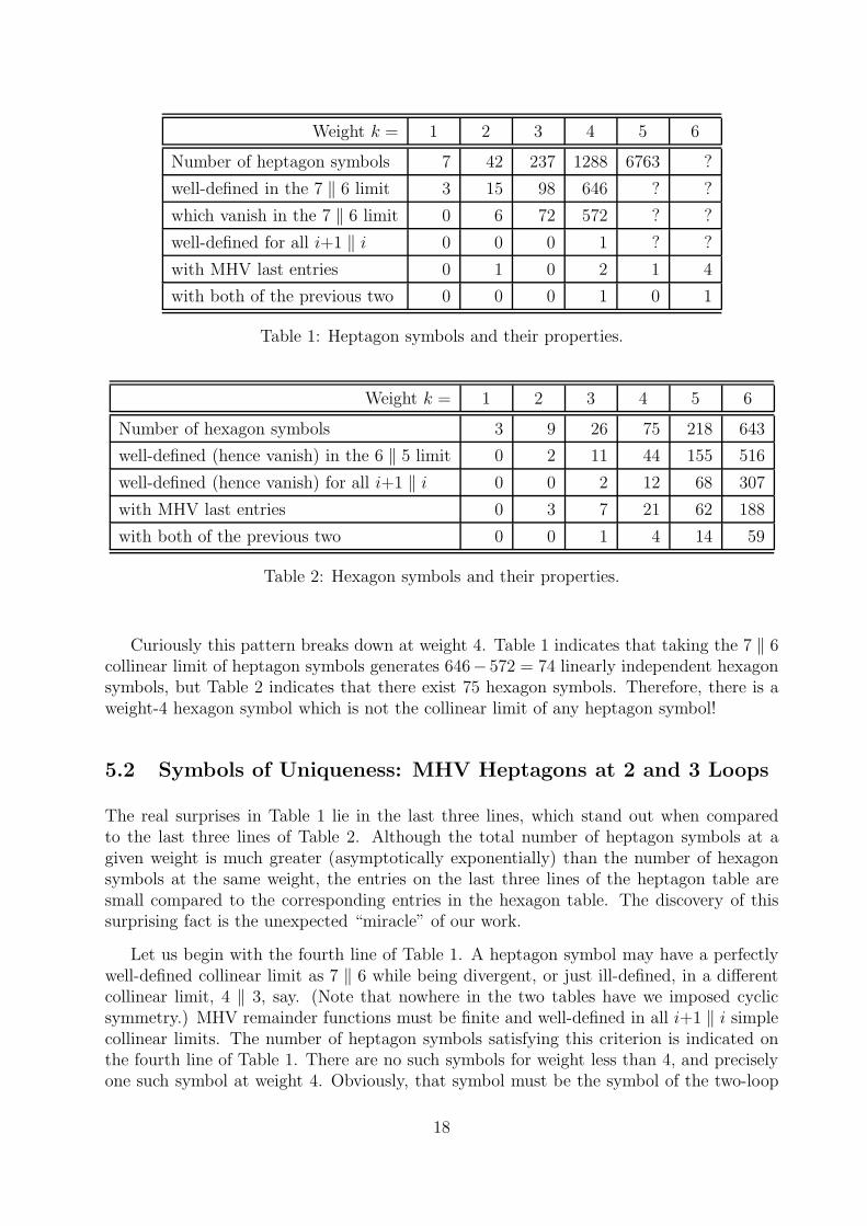
Weight k = 1 2 3 4 5 6

Number of heptagon symbols 7 42 237 1288 6763 ?

well-defined in the 7 ‖ 6 limit 3 15 98 646 ? ?

which vanish in the 7 ‖ 6 limit 0 6 72 572 ? ?

well-defined for all i+1 ‖ i 0 0 0 1 ? ?

with MHV last entries 0 1 0 2 1 4

with both of the previous two 0 0 0 1 0 1

Table 1: Heptagon symbols and their properties.

Weight k = 1 2 3 4 5 6

Number of hexagon symbols 3 9 26 75 218 643

well-defined (hence vanish) in the 6 ‖ 5 limit 0 2 11 44 155 516

well-defined (hence vanish) for all i+1 ‖ i 0 0 2 12 68 307

with MHV last entries 0 3 7 21 62 188

with both of the previous two 0 0 1 4 14 59

Table 2: Hexagon symbols and their properties.

Curiously this pattern breaks down at weight 4. Table 1 indicates that taking the 7 ‖ 6collinear limit of heptagon symbols generates 646− 572 = 74 linearly independent hexagonsymbols, but Table 2 indicates that there exist 75 hexagon symbols. Therefore, there is aweight-4 hexagon symbol which is not the collinear limit of any heptagon symbol!

5.2 Symbols of Uniqueness: MHV Heptagons at 2 and 3 Loops

The real surprises in Table 1 lie in the last three lines, which stand out when comparedto the last three lines of Table 2. Although the total number of heptagon symbols at agiven weight is much greater (asymptotically exponentially) than the number of hexagonsymbols at the same weight, the entries on the last three lines of the heptagon table aresmall compared to the corresponding entries in the hexagon table. The discovery of thissurprising fact is the unexpected “miracle” of our work.

Let us begin with the fourth line of Table 1. A heptagon symbol may have a perfectlywell-defined collinear limit as 7 ‖ 6 while being divergent, or just ill-defined, in a differentcollinear limit, 4 ‖ 3, say. (Note that nowhere in the two tables have we imposed cyclicsymmetry.) MHV remainder functions must be finite and well-defined in all i+1 ‖ i simplecollinear limits. The number of heptagon symbols satisfying this criterion is indicated onthe fourth line of Table 1. There are no such symbols for weight less than 4, and preciselyone such symbol at weight 4. Obviously, that symbol must be the symbol of the two-loop

18

seven-particle MHV remainder function R(2)7 ! To recap:

The symbol of the two-loop seven-particle MHV remainder function R(2)7 is the only

weight-4 heptagon symbol which is well-defined in all i+1 ‖ i collinear limits.

Let us emphasise that it is not necessary to assume dihedral symmetry, parity symmetry,or the last-entry condition. Nor is it necessary to use the expected collinear limit R

(2)6 as an

input to fix some remaining ambiguity (except for the overall multiplicative normalisation).All of these properties are automatically satisfied by the unique function described in theabove box. Of course, we have checked that the symbol of the function obtained in thismanner via the bootstrap programme indeed is proportional to the known symbol of R

(2)7

found in [65].

It would be extremely interesting to see if this criterion continues to hold at weight 6,i.e. to see whether the question mark in the last column of the fourth line of Table 1 is also1, but we have not yet completed this calculation. Nevertheless we note that this criterioncertainly could not work at arbitrary loop order; for example at weight 8 the square of R

(2)7

and the four-loop seven-particle MHV remainder function R(4)7 are both well-defined in all

simple collinear limits, and are distinct.

Let us now turn to the last two lines of Table 1, where we impose the last-entry conditionappropriate for MHV amplitudes, as discussed in section 3.1. In contrast to the generalheptagon problem, where the complexity of the linear systems involved has forced us toleave some questions marks in the table, when we impose the last-entry condition the sizeof the linear systems becomes “small” enough that we have succeeded in a full classificationthrough weight 6. This is certainly not to say that the calculation was easy—as explainedin section 4, determining the number “4” in the last column of Table 1 required finding thenullspace of a linear system with over half a million variables.

The number of heptagon symbols satisfying the last-entry condition is shown in thesixth line of Table 1. Let us note right away that none of the numbers are multiples of 7,hence all of these functions are necessarily cyclically invariant, even though this was not aninput to the calculation. Also it turns out (this is trivial at weights 2 and 5, where there isa single symbol, and is easily checked at weights 4 and 6) that they are all invariant underthe full dihedral group, as well as under the parity operation shown in eq. (20). Again noneof these discrete symmetries were imposed going into the calculation.

At weight 2 we find there is a unique heptagon symbol satisfying the last-entry condition.The corresponding heptagon function is written explicitly, and discussed in more detail, inthe following section. At weight 4 there are two functions: the square of the weight-2function, and the two-loop MHV remainder function R

(2)7 . As we have already seen, the

latter is the only one which is well-defined in all collinear limits. At weight 5 there is againa unique symbol satisfying the last-entry condition. This weight-5 symbol, like the weight-2symbol, is not well-defined in the collinear limit, so these two symbols have no role to playin connection with MHV scattering amplitudes.

Let us now focus again on the surprising “4” in the last column of Table 1. From

19

our discussion so far we already know that there must be at least two weight-6 heptagonfunctions satisfying the last-entry condition: the cube of the weight-2 function discussedabove, and the product of the weight-2 function with R

(2)7 . The surprise is that, in addition

to the symbols of these two functions, we find only two irreducible symbols at weight 6. Wefind that there is a unique linear combination of these four symbols which is finite in thecollinear limit (in this case it happens that it is sufficient to consider only the 7 ‖ 6 collinearlimit since, as mentioned above, the symbols turn out to all be cyclically invariant anyway).We have checked that the collinear limit matches perfectly (up to an overall factor, whichis not fixed by the bootstrap) the known symbol of the three-loop MHV hexagon [16, 59].Therefore:

The symbol of the three-loop seven-particle MHV remainder function R(3)7 is the

only weight-6 heptagon symbol which satisfies the last-entry condition and which isfinite in the 7 ‖ 6 collinear limit.

The only ambiguity which will be left when passing from the symbol of R(3)7 to an actual

function is the addition of a rational linear combination of ζ2R(2)7 , ζ23 and ζ6. The collinear

limit will fix all three coefficients (as well as the overall normalisation of R(3)7 ) uniquely.

Again we emphasise that the above conclusion does not rely on assuming that any of thediscrete symmetries are satisfied; they all emerge as “accidental” (if there is such a thing inSYM theory) properties of the unique solution. Moreover, and even more surprisingly, theunique solution emerges without any free parameters which need to be tuned in order tomatch the correct value of the three-loop MHV hexagon in the collinear limit, let alone tomatch various terms in the Regge limit and/or OPE expansion around the collinear limit.

6 Speculations: The n-gon Bootstrap at Weight 2

Our results were completely surprising. Based on the hexagon bootstrap programme, weexpected that even after imposing all discrete symmetries, there would likely be hundredsof free parameters in our heptagon ansatz which would need to be fit by comparison tovarious data in the literature.

The fact that none of this turned out to be necessary, and that the heptagon bootstrapturned out, in this sense, to be more powerful than the hexagon bootstrap, requires ex-planation. It is, after all, a basic tenet of amplitudeology that “accidents do not happen,”especially in SYM theory.

Unfortunately we have only very little to offer at this time. In this section we make afew meager observations at weight 2, where it is simple to tabulate and explicitly analyzethe relevant function spaces. Our observations here admittedly shed only a little light onthe situation at higher weight, but perhaps they serve as a useful starting point.

20

Let us define the cross-ratio

u1 =〈1256〉〈2345〉

〈1245〉〈2356〉=

a17a13a14

(32)

with six other ui defined cyclically (sometimes u1 is called u14 in the literature). Accordingto the sixth line of Table 1, there is a unique weight-2 heptagon function satisfying thelast-entry condition. This function is

7∑

i=1

Li2(1− 1/ui) +1

2log ui log

ui+2ui−2

ui+3uiui−3. (33)

Let us contrast this to the situation at n = 6, where there are three functions

Li2(1− 1/u) , Li2(1− 1/v) , Li2(1− 1/w) (34)

which separately satisfy the last-entry condition.

Why does this happen? The functions shown in eq. (34) exist because of the identity

1− u

u=〈1356〉〈2346〉

〈1236〉〈3456〉(35)

(and two cyclic images). Note that all of the brackets appearing on the right-hand sideare of the form 〈i j−1 j j+1〉. Hence all three of (1− u)/u, (1− v)/v, (1− w)/w are validMHV last entries.

Is there an analogue to the identity (35) for n = 7? That is, does there exist an identitywhich allows products of ui’s and 1− ui’s to be rewritten only in terms of 〈i j−1 j j+1〉’s?It is simple to check that there are precisely seven such identities:

1− u1

u1

1− u7

u7

1

1− u4

=〈1235〉〈1247〉〈1345〉〈2456〉

〈1234〉〈1257〉〈1456〉〈2345〉(36)

and its cyclic permutations. If it were not for the factor 1/(1 − u4) on the left, then thefunctions Li2(1−1/ui)+Li2(1−1/ui+1) would satisfy both the first- and last-entry conditionsfor all i. Instead, only the particular linear combination shown in eq. (33) is allowed.

It is straightforward to extend this analysis to higher n. The total number of weight-2n-gon functions grows very rapidly (in fact, as O(n4)) with n. How many of those functionssatisfy the last-entry condition? Obviously, it is to be expected that there should be verystrong interplay between the first- and last-entry conditions at weight 2, but we find anunexpectedly strong result:

We find that there are precisely 3 n-gon functions at weight 2 satisfying the last-entrycondition when n = 6 or when n is a multiple of four. For all other n, we find that there isonly one such function!

As we go to higher weight we might expect the interplay between the first- and last-entry conditions to become less constraining. This expectation may or may not turn outto be true asymptotically at large weight, but Tables 1 and 2 indicate little weakening ofthis interplay for k even as high as 6. Clearly it would be interesting to map out the spaceof n-gon functions at higher weight.

21

7 Discussion

We have found that the heptagon bootstrap for computing (symbols of) seven-point MHVamplitudes in SYM is unreasonably effective in comparison with the hexagon bootstrap,at least through three loops. In particular, the three-loop heptagon remainder function isthe unique weight-6 heptagon function which satisfies the last-entry condition and whichis finite in the 7 ‖ 6 collinear limit. Evidently the conceptually simplest way of computingthe three-loop hexagon remainder function is, somewhat perversely, to first compute theheptagon remainder and take its collinear limit.

Naturally, it would be very interesting to further explore the power of the heptagonbootstrap at higher loops or by relaxing the last-entry condition to those appropriate forNMHV amplitudes. It would also be interesting to explore the n-gon bootstrap for highern. Our analysis at weight-2 in section 6 suggests that the first- and last-entry conditions aremuch tighter in combination than each is individually. It would be important to understandwhether this is an accident at weight-2 (and whether the success of our heptagon bootstrapwas similarly accidental), or whether there is some fundamental feature of the structure ofn-gon functions which currently evades our understanding.

The cases n = 6, 7 are special because we believe that we know the appropriate symbolalphabets for amplitudes (both MHV and non-MHV) to all loop order, based on the factthat the associated cluster algebras have finitely many A-coordinates. However startingat n = 8 their number is infinite, so there is the possibility that new, more exotic symbolletters could start appearing at each loop order (or even when we go from MHV to non-MHV at a given loop order). Anything we could learn about the pattern of symbol letterswhich appear at higher n and at higher weight would be very valuable.

In section 5 we found an indication that thinking about the collinear limits of n-gonfunctions may lead to a class of previously underappreciated constraints. Specifically wefound that there exists a hexagon function at weight 4 which is not the collinear limit of anyheptagon function. Similarly, it is natural to expect that there may be heptagon functionswhich are not the collinear limit of any octagon functions, that there are hexagon functionswhich are not the double-collinear limit of any octagon function, etc. In this way we see thatthe consistency of collinear limits places an entire infinite tower of potentially very powerfulconstraints on the bootstrap. Along these lines, it has recently been shown [82] that thecollinear limit, together with dihedral symmetry and the first- and last-entry conditions,uniquely fixes the two-loop n-point MHV amplitude modulo classical polylogarithm func-tions for all n. The results of this paper suggest that even full symbols, if not full functions(which we have not addressed), may be surprisingly accessible via the n-gon bootstrap.

Finally, it is of course important to construct a complete functional representation forR

(3)7 . This would require first constructing a heptagon function of weight 6 with the correct

symbol, obeying the differential Q constraint and finite in the collinear limit. After thisthere will be beyond-the-symbol ambiguities corresponding to the addition of a numericalconstant (in particular a linear combination of ζ23 and ζ6) as well as a term proportional

to ζ2R(2)7 . Both of these ambiguities will be uniquely fixed by the simple collinear limit.

Having an explicit functional form for R(3)7 would not only allow for detailed checks against

22

the available predictions for its behaviour in the collinear [31, 33] and multi-Regge limits [51,52, 53], but would also shed light on yet unknown key quantities in these approaches. Theseinclude multi-particle scalar and fermion pentagon transitions, or higher BFKL eigenvalues,impact factors and central emission vertices. For example it would be great if our resultcould guide the generalisation of the all-loop formulas for the hexagon in the multi-Reggelimit [41], to the heptagon. The continuation of this programme for n = 8 will have aneven more interesting interplay with the BFKL approach, where a new bound state ofthree reggeised gluons first appears, and could moreover push forward our knowledge of thestrong coupling behaviour of the amplitudes [93, 94].

Acknowledgements

We thank B. Basso, S. Caron-Huot, L. Dixon, A. Sever and P. Vieira for comments onthe draft, and acknowledge having benefitted from stimulating discussions with J. Golden,E. Sokatchev and A. Volovich. The work of GP was supported by the French NationalAgency for Research (ANR) under contract StrongInt (BLANC-SIMI-4-2011). The workof MS was supported by the US Department of Energy under contract DE-SC0010010. MSis also grateful to the CERN theory group for their hospitality and support.

References

[1] L. Brink, J. H. Schwarz, and J. Scherk, Supersymmetric Yang-Mills Theories,Nucl.Phys. B121 (1977) 77.

[2] R. J. Eden, P. V. Landshoff, D. I. Olive, and J. C. Polkinghorne, The AnalyticS-Matrix. Cambridge University Press, 1966.

[3] L. F. Alday and J. M. Maldacena, Gluon scattering amplitudes at strong coupling,JHEP 0706 (2007) 064, [arXiv:0705.0303].

[4] J. Drummond, G. Korchemsky, and E. Sokatchev, Conformal properties of four-gluonplanar amplitudes and Wilson loops, Nucl.Phys. B795 (2008) 385–408,[arXiv:0707.0243].

[5] A. Brandhuber, P. Heslop, and G. Travaglini, MHV amplitudes in N = 4 superYang-Mills and Wilson loops, Nucl.Phys. B794 (2008) 231–243, [arXiv:0707.1153].

[6] J. Drummond, J. Henn, G. Korchemsky, and E. Sokatchev, On planar gluonamplitudes/Wilson loops duality, Nucl.Phys. B795 (2008) 52–68, [arXiv:0709.2368].

[7] J. Drummond, J. Henn, G. Korchemsky, and E. Sokatchev, Conformal Wardidentities for Wilson loops and a test of the duality with gluon amplitudes, Nucl.Phys.B826 (2010) 337–364, [arXiv:0712.1223].

23

[8] Z. Bern, L. Dixon, D. Kosower, R. Roiban, M. Spradlin, et al., The Two-LoopSix-Gluon MHV Amplitude in Maximally Supersymmetric Yang-Mills Theory,Phys.Rev. D78 (2008) 045007, [arXiv:0803.1465].

[9] J. Drummond, J. Henn, G. Korchemsky, and E. Sokatchev, Hexagon Wilson loop =six-gluon MHV amplitude, Nucl.Phys. B815 (2009) 142–173, [arXiv:0803.1466].

[10] J. Drummond, J. Henn, V. Smirnov, and E. Sokatchev, Magic identities forconformal four-point integrals, JHEP 0701 (2007) 064, [hep-th/0607160].

[11] Z. Bern, M. Czakon, L. J. Dixon, D. A. Kosower, and V. A. Smirnov, The Four-LoopPlanar Amplitude and Cusp Anomalous Dimension in Maximally SupersymmetricYang-Mills Theory, Phys.Rev. D75 (2007) 085010, [hep-th/0610248].

[12] Z. Bern, J. Carrasco, H. Johansson, and D. Kosower, Maximally supersymmetricplanar Yang-Mills amplitudes at five loops, Phys.Rev. D76 (2007) 125020,[arXiv:0705.1864].

[13] L. F. Alday and J. Maldacena, Comments on gluon scattering amplitudes viaAdS/CFT, JHEP 0711 (2007) 068, [arXiv:0710.1060].

[14] V. Del Duca, C. Duhr, and V. A. Smirnov, The Two-Loop Hexagon Wilson Loop inN = 4 SYM, JHEP 1005 (2010) 084, [arXiv:1003.1702].

[15] A. B. Goncharov, M. Spradlin, C. Vergu, and A. Volovich, Classical Polylogarithmsfor Amplitudes and Wilson Loops, Phys.Rev.Lett. 105 (2010) 151605,[arXiv:1006.5703].

[16] L. J. Dixon, J. M. Drummond, and J. M. Henn, Bootstrapping the three-loop hexagon,JHEP 1111 (2011) 023, [arXiv:1108.4461].

[17] L. J. Dixon, J. M. Drummond, and J. M. Henn, Analytic result for the two-loopsix-point NMHV amplitude in N = 4 super Yang-Mills theory, JHEP 1201 (2012)024, [arXiv:1111.1704].

[18] L. J. Dixon, J. M. Drummond, M. von Hippel, and J. Pennington, Hexagon functionsand the three-loop remainder function, JHEP 1312 (2013) 049, [arXiv:1308.2276].

[19] L. J. Dixon, J. M. Drummond, C. Duhr, and J. Pennington, The four-loop remainderfunction and multi-Regge behavior at NNLLA in planar N = 4 super-Yang-Millstheory, JHEP 1406 (2014) 116, [arXiv:1402.3300].

[20] L. J. Dixon, J. M. Drummond, C. Duhr, M. von Hippel, and J. Pennington,Bootstrapping six-gluon scattering in planar N = 4 super-Yang-Mills theory, PoSLL2014 (2014) 077, [arXiv:1407.4724].

[21] L. J. Dixon and M. von Hippel, Bootstrapping an NMHV amplitude through threeloops, JHEP 1410 (2014) 65, [arXiv:1408.1505].

24

[22] C. Anastasiou, Z. Bern, L. J. Dixon, and D. Kosower, Planar amplitudes inmaximally supersymmetric Yang-Mills theory, Phys.Rev.Lett. 91 (2003) 251602,[hep-th/0309040].

[23] Z. Bern, L. J. Dixon, and V. A. Smirnov, Iteration of planar amplitudes in maximallysupersymmetric Yang-Mills theory at three loops and beyond, Phys.Rev. D72 (2005)085001, [hep-th/0505205].

[24] V. Nair, A Current Algebra for Some Gauge Theory Amplitudes, Phys.Lett. B214

(1988) 215.

[25] S. J. Parke and T. Taylor, An Amplitude for n Gluon Scattering, Phys.Rev.Lett. 56(1986) 2459.

[26] L. F. Alday, D. Gaiotto, J. Maldacena, A. Sever, and P. Vieira, An Operator ProductExpansion for Polygonal null Wilson Loops, JHEP 1104 (2011) 088,[arXiv:1006.2788].

[27] D. Gaiotto, J. Maldacena, A. Sever, and P. Vieira, Bootstrapping Null PolygonWilson Loops, JHEP 1103 (2011) 092, [arXiv:1010.5009].

[28] D. Gaiotto, J. Maldacena, A. Sever, and P. Vieira, Pulling the straps of polygons,JHEP 1112 (2011) 011, [arXiv:1102.0062].

[29] A. Sever and P. Vieira, Multichannel Conformal Blocks for Polygon Wilson Loops,JHEP 1201 (2012) 070, [arXiv:1105.5748].

[30] B. Basso, A. Sever, and P. Vieira, Spacetime and Flux Tube S-Matrices at FiniteCoupling for N = 4 Supersymmetric Yang-Mills Theory, Phys.Rev.Lett. 111 (2013),no. 9 091602, [arXiv:1303.1396].

[31] B. Basso, A. Sever, and P. Vieira, Space-time S-matrix and Flux tube S-matrix II.Extracting and Matching Data, JHEP 1401 (2014) 008, [arXiv:1306.2058].

[32] B. Basso, A. Sever, and P. Vieira, Space-time S-matrix and Flux-tube S-matrix III.The two-particle contributions, JHEP 1408 (2014) 085, [arXiv:1402.3307].

[33] B. Basso, A. Sever, and P. Vieira, Space-time S-matrix and Flux-tube S-matrix IV.Gluons and Fusion, JHEP 1409 (2014) 149, [arXiv:1407.1736].

[34] A. Belitsky, Nonsinglet pentagons and NHMV amplitudes, arXiv:1407.2853.

[35] A. Belitsky, Fermionic pentagons and NMHV hexagon, arXiv:1410.2534.

[36] B. Basso, J. Caetano, L. Cordova, A. Sever, and P. Vieira, OPE for all HelicityAmplitudes, arXiv:1412.1132.

[37] G. Papathanasiou, Hexagon Wilson Loop OPE and Harmonic Polylogarithms, JHEP1311 (2013) 150, [arXiv:1310.5735].

[38] G. Papathanasiou, Evaluating the six-point remainder function near the collinearlimit, Int.J.Mod.Phys. A29 (2014), no. 27 1450154, [arXiv:1406.1123].

25

[39] J. M. Drummond and G. Papathanasiou, “Hexagon from collinear to multi-Reggekinematics.” To appear.

[40] N. Beisert, C. Ahn, L. F. Alday, Z. Bajnok, J. M. Drummond, et al., Review ofAdS/CFT Integrability: An Overview, Lett.Math.Phys. 99 (2012) 3–32,[arXiv:1012.3982].

[41] B. Basso, S. Caron-Huot, and A. Sever, Adjoint BFKL at finite coupling: a short-cutfrom the collinear limit, arXiv:1407.3766.

[42] J. Bartels, L. Lipatov, and A. Sabio Vera, BFKL Pomeron, Reggeized gluons andBern-Dixon-Smirnov amplitudes, Phys.Rev. D80 (2009) 045002, [arXiv:0802.2065].

[43] J. Bartels, L. Lipatov, and A. Sabio Vera, N = 4 supersymmetric Yang Millsscattering amplitudes at high energies: The Regge cut contribution, Eur.Phys.J. C65

(2010) 587–605, [arXiv:0807.0894].

[44] L. Lipatov and A. Prygarin, Mandelstam cuts and light-like Wilson loops in N = 4SUSY, Phys.Rev. D83 (2011) 045020, [arXiv:1008.1016].

[45] L. Lipatov and A. Prygarin, BFKL approach and six-particle MHV amplitude inN = 4 super Yang-Mills, Phys.Rev. D83 (2011) 125001, [arXiv:1011.2673].

[46] J. Bartels, L. Lipatov, and A. Prygarin, MHV Amplitude for 3→3 Gluon Scatteringin Regge Limit, Phys.Lett. B705 (2011) 507–512, [arXiv:1012.3178].

[47] V. Fadin and L. Lipatov, BFKL equation for the adjoint representation of the gaugegroup in the next-to-leading approximation at N = 4 SUSY, Phys.Lett. B706 (2012)470–476, [arXiv:1111.0782].

[48] A. Prygarin, M. Spradlin, C. Vergu, and A. Volovich, All Two-Loop MHV Amplitudesin Multi-Regge Kinematics From Applied Symbology, Phys.Rev. D85 (2012) 085019,[arXiv:1112.6365].

[49] L. Lipatov, A. Prygarin, and H. J. Schnitzer, The Multi-Regge limit of NMHVAmplitudes in N = 4 SYM Theory, JHEP 1301 (2013) 068, [arXiv:1205.0186].

[50] L. J. Dixon, C. Duhr, and J. Pennington, Single-valued harmonic polylogarithms andthe multi-Regge limit, JHEP 1210 (2012) 074, [arXiv:1207.0186].

[51] J. Bartels, A. Kormilitzin, L. Lipatov, and A. Prygarin, BFKL approach and 2→ 5maximally helicity violating amplitude in N = 4 super-Yang-Mills theory, Phys.Rev.D86 (2012) 065026, [arXiv:1112.6366].

[52] J. Bartels, A. Kormilitzin, and L. Lipatov, Analytic structure of the n = 7 scatteringamplitude in N = 4 SYM theory at multi-Regge kinematics: Conformal Regge polecontribution, Phys.Rev. D89 (2014) 065002, [arXiv:1311.2061].

[53] J. Bartels, A. Kormilitzin, and L. N. Lipatov, Analytic structure of the n = 7scattering amplitude in N = 4 SYM theory in multi-Regge kinematics: ConformalRegge cut contribution, arXiv:1411.2294.

26

[54] J. Drummond, J. Henn, G. Korchemsky, and E. Sokatchev, Dual superconformalsymmetry of scattering amplitudes in N = 4 super-Yang-Mills theory, Nucl.Phys.B828 (2010) 317–374, [arXiv:0807.1095].

[55] L. Mason and D. Skinner, The Complete Planar S-matrix of N = 4 SYM as a WilsonLoop in Twistor Space, JHEP 1012 (2010) 018, [arXiv:1009.2225].

[56] S. Caron-Huot, Notes on the scattering amplitude / Wilson loop duality, JHEP 1107

(2011) 058, [arXiv:1010.1167].

[57] T. Adamo, M. Bullimore, L. Mason, and D. Skinner, Scattering Amplitudes andWilson Loops in Twistor Space, J.Phys. A44 (2011) 454008, [arXiv:1104.2890].

[58] M. Bullimore and D. Skinner, Descent Equations for Superamplitudes,arXiv:1112.1056.

[59] S. Caron-Huot and S. He, Jumpstarting the All-Loop S-Matrix of Planar N = 4Super Yang-Mills, JHEP 1207 (2012) 174, [arXiv:1112.1060].

[60] J. M. Drummond, J. M. Henn, and J. Plefka, Yangian symmetry of scatteringamplitudes in N = 4 super Yang-Mills theory, JHEP 0905 (2009) 046,[arXiv:0902.2987].

[61] J. Drummond and L. Ferro, Yangians, Grassmannians and T-duality, JHEP 1007

(2010) 027, [arXiv:1001.3348].

[62] V. Del Duca, C. Duhr, and V. A. Smirnov, An Analytic Result for the Two-LoopHexagon Wilson Loop in N = 4 SYM, JHEP 1003 (2010) 099, [arXiv:0911.5332].

[63] V. Del Duca, C. Duhr, and V. A. Smirnov, A Two-Loop Octagon Wilson Loop inN = 4 SYM, JHEP 1009 (2010) 015, [arXiv:1006.4127].

[64] P. Heslop and V. V. Khoze, Analytic Results for MHV Wilson Loops, JHEP 1011

(2010) 035, [arXiv:1007.1805].

[65] S. Caron-Huot, Superconformal symmetry and two-loop amplitudes in planar N = 4super Yang-Mills, JHEP 1112 (2011) 066, [arXiv:1105.5606].

[66] J. Golden, A. B. Goncharov, M. Spradlin, C. Vergu, and A. Volovich, MotivicAmplitudes and Cluster Coordinates, JHEP 1401 (2014) 091, [arXiv:1305.1617].

[67] S. Fomin and A. Zelevinsky, Cluster algebras I: Foundations, J. Am. Math. Soc. 15(2002), no. 2 497–529, [math/0104151].

[68] S. Fomin and A. Zelevinsky, Cluster algebras II: Finite type classification, Invent.Math. 154 (2003), no. 1 63–121, [math/0208229].

[69] A. Goncharov, Multiple polylogarithms and mixed Tate motives, math/0103059.

[70] A. B. Goncharov, Galois symmetries of fundamental groupoids and noncommutativegeometry, Duke Math. J. 128 (06, 2005) 209–284, [math/0208144].

27

[71] F. C. Brown, Multiple zeta values and periods of moduli spaces M0,n(R), AnnalesSci.Ecole Norm.Sup. 42 (2009) 371, [math/0606419].

[72] A. B. Goncharov, A simple construction of Grassmannian polylogarithms, Adv. Math.241 (2013) 79–102, [arXiv:0908.2238].

[73] C. Duhr, H. Gangl, and J. R. Rhodes, From polygons and symbols to polylogarithmicfunctions, JHEP 1210 (2012) 075, [arXiv:1110.0458].

[74] C. Duhr, Hopf algebras, coproducts and symbols: an application to Higgs bosonamplitudes, JHEP 1208 (2012) 043, [arXiv:1203.0454].

[75] J. Golden and M. Spradlin, The differential of all two-loop MHV amplitudes in N =4 Yang-Mills theory, JHEP 1309 (2013) 111, [arXiv:1306.1833].

[76] J. Golden, M. F. Paulos, M. Spradlin, and A. Volovich, Cluster Polylogarithms forScattering Amplitudes, arXiv:1401.6446.

[77] J. Golden and M. Spradlin, An analytic result for the two-loop seven-point MHVamplitude in N = 4 SYM, JHEP 1408 (2014) 154, [arXiv:1406.2055].

[78] V. V. Fock and A. B. Goncharov, Cluster ensembles, quantization and thedilogarithm, Ann. Sci. Ec. Norm. Super. (4) 42 (2009), no. 6 865–930,[math/0311245].

[79] A. Hodges, Eliminating spurious poles from gauge-theoretic amplitudes, JHEP 1305

(2013) 135, [arXiv:0905.1473].

[80] N. Arkani-Hamed, J. L. Bourjaily, F. Cachazo, A. B. Goncharov, A. Postnikov, et al.,Scattering Amplitudes and the Positive Grassmannian, arXiv:1212.5605.

[81] S. Caron-Huot and S. He, Three-loop octagons and n-gons in maximallysupersymmetric Yang-Mills theory, JHEP 1308 (2013) 101, [arXiv:1305.2781].

[82] J. Golden and M. Spradlin, A Cluster Bootstrap for Two-Loop MHV Amplitudes,arXiv:1411.3289.

[83] Z. Bern, L. J. Dixon, D. C. Dunbar, and D. A. Kosower, One loop n point gaugetheory amplitudes, unitarity and collinear limits, Nucl.Phys. B425 (1994) 217–260,[hep-ph/9403226].

[84] Z. Bern, J. Rozowsky, and B. Yan, Two loop four gluon amplitudes in N = 4superYang-Mills, Phys.Lett. B401 (1997) 273–282, [hep-ph/9702424].

[85] C. Anastasiou, A. Brandhuber, P. Heslop, V. V. Khoze, B. Spence, et al., Two-LoopPolygon Wilson Loops in N = 4 SYM, JHEP 0905 (2009) 115, [arXiv:0902.2245].

[86] K.-T. Chen, Iterated path integrals, Bull. Amer. Math. Soc. 83 (1977), no. 5 831–879.

[87] M. Kauers, Fast solvers for dense linear systems, Nucl.Phys.Proc.Suppl. 183 (2008)245–250.

28

[88] A. Storjohann, Algorithms for Matrix Canonical Forms. PhD thesis, Swiss FederalInstitute of Technology, ETH-Zurich, 2000.

[89] Z. Chen and A. Storjohann, A blas based c library for exact linear algebra on integermatrices, in Proceedings of the 2005 International Symposium on Symbolic andAlgebraic Computation, ISSAC ’05, (New York, NY, USA), pp. 92–99, ACM, 2005.

[90] V. Strassen, Gaussian elimination is not optimal, Numer. Math. 13 (1969), no. 4354–356.

[91] Arne Storjohann, Faster Algorithms for Integer Lattice Basis Reduction, 1996.

[92] V. Velizhanin, Four loop anomalous dimension of the third and fourth moments ofthe non-singlet twist-2 operator in QCD, arXiv:1411.1331.

[93] J. Bartels, V. Schomerus, and M. Sprenger, Heptagon Amplitude in the Multi-ReggeRegime, JHEP 1410 (2014) 67, [arXiv:1405.3658].

[94] J. Bartels, V. Schomerus, and M. Sprenger, The Bethe Roots of Regge Cuts inStrongly Coupled N = 4 SYM Theory, arXiv:1411.2594.

29