force control for robotic manipulators with - circle
TRANSCRIPT

FORCE CONTROL FOR ROBOTIC MANIPULATORS
WITH STRUCTURALLY FLEXIBLE LINKS
By
Douglas John Latornell
B.Sc. ions. (Mechanical Engineering) Queen’s University
M.Sc. (Mechanical Engineering) Queen’s University
A THESIS SUBMITTED IN PARTIAL FULFILLMENT OF
THE REQUIREMENTS FOR THE DEGREE OF
DOCTOR OF PHILOSOPHY
in
THE FACULTY OF GRADUATE STUDIES
DEPARTMENT OF MECHANICAL ENGINEERING
We accept this thesis as conforming
to the required standard
THE UNIVERSITY OF BRITISH COLUMBIA
1992
© Douglas John Latornell, 14 August 1992

In presenting this thesis in partial fulfilment of the requirements for an advanced
degree at the University of British Columbia, I agree that the Library shall make it
freely available for reference and study. I further agree that permission for extensive
copying of this thesis for scholarly purposes may be granted by the head of my
department or by his or her representatives. It is understood that copying or
publication of this thesis for financial gain shall not be allowed without my written
permission.
________________________________
Department of / iç7
The University of British ColumbiaVancouver, Canada
Date aki /92
DE-6 (2/88)

Abstract
This thesis reports on the development of strategies for the control of contact forces exerted
by a structurally flexible robotic manipulator on surfaces in its working environment. The
controller is based on a multivariable, explicitly adaptive, long range predictive control
algorithm. A static equilibrium bias term which is particularly applicable to the contact
force control problem has been incorporated into the control algorithm cost function. A
general formulation for the discrete time domain characteristic polynomial of the closed
loop system has been derived and shown useful in tuning the controller.
Kinematic and dynamic models of a robotic manipulator with structurally flexible links
interacting with its working environment are derived. These models include inertia and
damping effects in the contact dynamics in addition to the contact stiffness employed in
most previous work. Linear analyses of the dynamic models for a variety of manipulator
configurations reveal that the controlled variable, the contact force, is dominated by different
open ioop modes of the system depending on the effective stiffness of the contacting surfaces.
This result has important implications for the selection of the controller parameters.
The performance of the controller has been evaluated using computer simulation. A
special purpose simulation program, TWOFLEX, which includes the dynamics models of the
manipulator and the environment as well as the control algorithm was developed during
the research. The configurations investigated using the simulation include a single flexible
manipulator link, two link manipulators with both rigid and flexible links, and a two link
prototype model of the Mobile Servicing System (MS S) manipulator for the proposed Space
Station, Freedom. The results show that the controller can be tuned to provide fast contact
force step responses with minimal overshoot and zero steady-state error. The problem of
11

maintaining control through the discontinuous situation of unexpectedly making contact
with a surface is addressed with the introduction of a contact control logic level in the
control hierarchy.
111

Abstract
List of Tables
Table of Contents
11
vi”
List of Figures
Nomenclature
Acknowledgements
1 Introduction
1.1 Introduction
1.2 Motivation
1.3 Survey of Related Research
1.4 Contributions of the Thesis
1.5 Outline of the Thesis . .
x
xvi
xxv
2 Manipulator Modelling
2.1 Introduction
2.2 Literature Review
2.3 Kinematics
2.3.1 Manipulator Configuration
2.3.2 Flexible Link Model .
2.3.3 Contact Model
14
14
15
19
19
25
29
1
1
2
3
6
9
Model .
iv

2.4 Derivation of Equations of Motion 32
2.5 Contact Force Model 48
2.5.1 Hertz Contact Model 52
2.6 Voltage Controlled DC Electric Motor Actuator Model 54
2.7 Summary 58
3 Control Algorithm 59
3.1 Introduction 59
3.2 Review of SISO GPC Algorithm 62
3.2.1 Control Law Structure and Closed Loop Characteristics 66
3.3 Multivariable Predictive Control Algorithm 69
3.3.1 Control Law Structure and Closed Loop Characteristics 76
3.4 Static Equilibrium Bias Term 79
3.5 Control Algorithm Parameters and Tuning 83
3.6 Parameter Estimation 86
3.7 Adaptive Controller Implementation 90
3.8 Stability and Convergence 92
3.9 Summary 93
4 Dynamics and Control Simulation — TWOFLEX 95
4.1 Introduction 95
4.2 General Description of the TWOFLEX Program 96
4.3 Integration of Equations of Motion 99
4.4 Discrete Time Control Algorithm 102
4.5 Validation 106
4.6 Summary 109
v

111
• • • . 111
• • • . 114
• • 114
• • • . 121
• • • • 135
• 135
• • 136
• • • . 137
• • 141
• • • . 151
• . . • 160
• . . . 163
• . . . 166
• • . . 169
• . . . 174
• . . . 175
• . • . 197
• . . . 199
202
• . . . 217
• . . . 218
• . . . 224
6 Summary of Major Results
6.1 Recommendations for Further Research
5 Force Control Algorithm Performance and Evaluation
5.1 Introduction
5.2 Linear Analysis
5.2.1 Rigid Link
5.2.2 Flexible Link
5.3 Force Control for a Single Flexible Link
5.3.1 Link Model Parameters
5.3.2 Controller Model
5.3.3 Soft Contact Case (keff 3.lkN/m)
5.3.4 Hertz Contact Model Case (kff 5MN/m)
5.3.5 keff = 62kN/m Contact Stiffness Case .
5.3.6 Summary
5.4 Making and Breaking Contact
5.4.1 Stop Motion Strategy
5.4.2 Force Setpoint Modification Strategy .
5.5 Force Control for Two Link Manipulators
5.5.1 Linear Analysis
5.5.2 Controller Model
5.5.3 Force Control for Two Rigid Links . .
5.5.4 Force Control for Two Flexible Links . .
5.5.5 Summary
5.6 Force Control for DC Motor Actuated Space Station Manipulator
5.7 Summary of Force Control Performance
228
231
vi

Bibliography
Appendices
235
242
A Equations of Motion for Various Manipulator Configurations
A.1 Planar Two Link Flexible Manipulator in Free Motion
A.2 Planar Two Rigid Link Manipulator in Contact
A.3 Planar Two Link Rigid Manipulator in Free Motion
A.4 One Flexible Link in Contact
A.5 One Flexible Link in Free Motion
A.6 One Rigid Link in Contact
A.7 DC Motor Actuated Single Flexible Link in Free Motion
242
242
245
247
248
249
249
250
B Cost Function Expansions
B.1 Multivariable Predictive Control Algorithm
B.2 Static Equilibrium Bias Term
C Static Equilibrium Function Derivation 253
251
• 251
• 252
vii

List of Tables
4.1 Configurations and initial conditions for validation of inertia matrix and right
hand side vector terms 107
4.2 Configurations and initial conditions for free response simulation validation
runs 107
5.1 Mode shape function integral factor values for a single flexible link with one
structural mode 123
5.2 Natural frequencies and mode shape function integral factor values for single
flexible link run 136
5.3 Material properties and Hertz model parameters for steel on aluminium contact 142
5.4 Stabilising controller horizons and closed ioop characteristics for steel on
aluminium contact (keff = 5.0037MN/m) for a single flexible link with one
structural mode 146
5.5 Stabilising controller horizons and closed ioop characteristics for steel on
aluminium contact (keff = 61.554kN/m) with a single flexible link with one
structural mode 153
5.6 Stabilising controller horizons and closed ioop characteristics for steel on
aluminium contact (keff = 61.554kN/m) with a single flexible link with three
structural modes 160
5.7 Parameter values for two rigid link manipulator controller model 200
5.8 Stabilising controller horizons and closed ioop characteristics for a struc
turally rigid two link manipulator contacting a keff = kN/m surface 202
viii

5.9 Parameter values for two flexible link manipulator controller model 204
5.10 Stabilising controller horizons and closed ioop characteristics for a two flexible
link (one structural mode each) manipulator contacting a keff = lOkN/m
surface 208
5.11 Physical parameter values for a two link MSS model with DC motor actuators.219
ix

List of Figures
2.1 Geometry of a two link flexible manipulator in contact with a deformable
surface 19
2.2 Coordinate frames for a two link flexible manipulator in contact with a de
formable surface 21
2.3 Free body diagram of a differential beam element 26
2.4 Axial foreshortening of a differential beam element 29
2.5 Manipulator—environment model for derivation of contact force expressions 49
2.6 Free body diagrams for the x direction contact region mass 50
2.7 Schematic of direct current motor actuator system 55
3.1 SISO GPC closed loop system block diagram 68
3.2 Comparison of EFRA and U/D RLS parameter estimation algorithms. . 89
3.3 Control strategy block diagram 91
4.1 Flowchart of the overall structure of the TWOFLEX dynamics and control sim
ulation program 97
4.2 Flowchart of the calculation of the generalised acceleration vector 102
4.3 Flowchart of the discrete time control algorithm 103
4.4 Comparison of joint angle responses for free response validation 108
4.5 Comparison of modal amplifier responses for free response validation 110
5.1 Topics discussed in Chapter 5 112
5.2 Single rigid link in contact with a deformable environment 114
x

5.3 Variation of the natural frequencies with effective contact stiffness for a single
rigid link/environment system 117
5.4 Single flexible link in contact with a deformable environment 121
5.5 Variation of the natural frequencies with effective contact stiffness for a single
flexible link with one structural mode 124
5.6 Single flexible link in contact with a deformable environment approximated
by a steady state contact dynamics model 125
5.7 Variation of the natural mode components of the contact force with effective
contact stiffness for a single flexible link with one structural mode 127
5.8 Variation with effective contact stiffness of the relative excitation of the nat
ural modes of a single flexible link with one structural mode in contact. . . 129
5.9 Variation with effective contact stiffness of system natural frequencies for a
soft link (El1 = 40N . m2) 130
5.10 Variation with effective contact stiffness of system natural frequencies for a
flexible link with four structural modes 132
5.11 Variation of the natural mode components of the contact force with effec
tive contact stiffness for a single flexible link (El1 = 200N . m2) with four
structural modes 133
5.12 Variation with effective contact stiffness of the relative excitation of the nat
ural modes of a single flexible link (El1 200N . m) with four structural
modes 134
5.13 Variation of natural frequencies of a single flexible link (El1 = 574N m2,
two structural modes) in contact 139
5.14 Contact force response of a single flexible link on a soft surface (k5 = ke =
6200N/m) 140
xi

5.15 Variation of natural frequencies of a single flexible link (with one structural
mode) in contact 145
5.16 Comparison of results from simulations using full contact dynamics and
steady state approximation 147
5.17 Force control step response for a single flexible link (with one structural
mode), steel on aluminium contact (keff = 5MN/m) with N2 = 20, N = 2,
= 0, and Age = 0 148
5.18 Force control step responses for a single flexible link (with one structural
mode), steel on aluminium contact (keff = 5MN/m) with 0 Age 0.4. . . 150
5.19 Experimental contact stiffness estimate for steel on aluminium 152
5.20 Force control step response for a single mode flexible link (with one structural
mode), steel on aluminium contact (kff = 61.554kN/m) with N2 = 10,
N=3,A=0,A8=0 154
5.21 Force control step response for a single mode flexible link (with one structural
mode), steel on aluminium contact (kff = 61.554kN/m) with N2 = 5, N.
4, A = 0, A = 0 155
5.22 Force control step response for a single flexible link (with one structural
mode), steel on aluminium contact (keff = 61.554kN/m) with N2 = 5, N
3, A = 0, Age 0 156
5.23 Force control step response for a single flexible link (with one structural
mode), steel on aluminium contact (keff = 61.554kN/m) with N2 = 7, N =
4,Ac0,A8e0 158
5.24 Variation of the natural frequencies of a single flexible link (El1 = 574N m2
with three structural modes) in contact 159
xii

5.25 Force control step response for single flexible link (with three structural
modes), steel on aluminium contact (keff = 61.554kN/m), with N2 = 8,
N, = 4, = 0, )ise = 0 161
5.26 Block diagram of the overall control structure 165
5.27 Joint angle and contact force responses for a single flexible link colliding with
a 6200N/m surface 167
5.28 Simple 1 degree of freedom model of a single link in contact with an environ
ment 170
5.29 Contact force response for a single flexible link making contact with a 6200N/m
surface at 0.536m/s 172
5.30 Contact force response of a single flexible link colliding with a 6200N/m
surface with force setpoint modification 173
5.31 Two rigid link manipulator in contact with a deformable environment . . . 176
5.32 Variation of the natural frequencies with effective contact stiffness for a two
rigid link manipulator in contact 178
5.33 and 2 mode shapes for various values of for a two rigid link manipulator.183
5.34 Variation of contact force components in natural coordinate space with O
with keff = 61.554kN/m 185
5.35 Relative excitation of the natural modes of a two link rigid manipulator by
the control inputs 187
5.36 Variation of the natural frequencies with effective contact stiffness of a two
link manipulator with identical, flexible (El = 574N m2, one structural
mode each) links in contact with an isotropic (kxeff kyeff) environment. . . 191
5.37 Variation of the natural frequencies with effective contact stiffness for a two
flexible link manipulator (El = 574N m2, one structural mode each) with
= 1.Om and L2 = 2.Om 193
xlii

5.38 Variation of the natural mode components of the contact forces with effective
contact stiffness for a two flexible link manipulator 195
5.39 Variation of the relative excitation of the natural modes with effective contact
stiffness for a two flexible link manipulator 196
5.40 Force control step responses for a structurally rigid two link manipulator
contacting a keff = lOkN/m surface with N2 = 5, Nu = 2, c = 0 203
5.41 Variation of the natural frequencies for a two link manipulator with identical
flexible links assuming steady state contact dynamics 206
5.42 Force control step responses for linear dynamics simulation of a two flexible
link (one structural mode each) manipulator contacting a keff = lOkN/m
surface with N2 20, N = 2, 0 209
5.43 Force control step responses for linear dynamics simulation of a two flexible
link (one structural mode each) manipulator contacting a keff = lOkN/m
surfacewithN2=8,N=4,)=0 211
5.44 Force control step responses showing output interactions for linear dynamics
simulation of a two flexible link (one structural mode each) manipulator
contacting a keff = lOkN/m surface with N2 = 20, N = 2, 0 212
5.45 Force control step responses showing output interactions for linear dynamics
simulation of a two flexible link (one structural mode each) manipulator
contacting a keff = lOkN/m surface with N2 = 8, N = 4, = 0 213
5.46 Force control step responses for nonlinear dynamics simulation of a two flexi
ble link (one structural mode each) manipulator contacting a keff = lOkN/m
surface with N2 = 20, N = 2, , = 0 215
5.47 Variation of the modal natural frequencies for DC motor actuated two link
MSS model 220
xiv

5.48 Force control responses for linear dynamics simulation of a two flexible link
Space Station MSS contacting a keff = 2OkN/m surface 222
5.49 Force control responses for nonlinear dynamics simulation of a two flexible
link Space Station MSS contacting a keff = 2OkN/m surface 223
xv

Nomenclature
Roman letters
A(q1) discrete time input/output model denominator polynomial of degree ma
a radius of circular contact area in the Hertz contact model
B(q’) discrete time input/output model numerator polynomial of degree mb
Bk(q’) discrete time input/output model numerator polynomial relating kth input toith output in a discrete time multivariable system model
ba equivalent viscous damping coefficient for DC motor armature frictional damping
bex equivalent viscous damping factor for contact damping of the environmentsurface in the x direction
bey equivalent viscous damping factor for contact damping of the environmentsurface in the y direction
bk, equivalent viscous damping factor for structural damping of mode i of link k
b3 equivalent viscous damping factor for contact damping of the manipulator tipsurface in the x direction
b3 equivalent viscous damping factor for contact damping of the manipulator tipsurface in the y direction
bek equivalent viscous damping factor for friction in joint k
c, vector of generalised coordinate components for linearised model of F
c, vector of generalised coordinate components for linearised model of F
c1 cosine of joint angle 1 (Ox)
c2 cosine of joint angle 2 (&2)
ca2 cosine of [w’10(t) + 2(t)]
Clai2 cosine of [61(t) + w0(t) + 2(t)]
xvi

D,(t) homogeneous transformation matrix to describe the structural deformation oflink 1 relative to coordinate frame
D2(t) homogeneous transformation matrix to describe the structural deformation oflink 2 relative to coordinate frame F2
D inverse of effective planar strain modulus in the Hertz contact model
d(t) disturbance term for ith output in a multivariable system model
dm, an element of mass on link 1
dm2 an element of mass on link 2
E matrix whose columns are the eigenvectors of a linear system
E(q’) a backward shift polynomial which satisfies the Diophantine identity
Ek modulus of elasticity of the material of surface k in the Hertz contact model
Elk fiexural rigidity of link k in bending about its joint axis
ê vector of optimal predictions of future output errors for the ith output of amultivariable system
ek eigenvector corresponding to the kth natural frequency of a linear system
F applied force in the Hertz contact model
F3(q’) a backward shift polynomial which satisfies the Diophantine identity
Fk peak contact force during collision transient
a direction component of contact force, relative to and projected onto F°
F y direction component of contact force, relative to and projected onto F°
F° fixed world coordinate frame with mutually perpendicular unit direction vectors; i, i and i
F’ coordinate frame for link 1 with mutually perpendicular unit direction vectors;i, i and i
F2 coordinate frame for link 2 with mutually perpendicular unit direction vectors;i, i and i
FC coordinate frame at the location of initial contact with mutually perpendicularunit direction vectors; i, i and i
xvii

f vector of q’ polynomial operators
f vector of free response components of the ith predicted output from time stept + 1 to t + N2; subscript is dropped in SISO case
f(t + j) free response part of (t + jt)
f natural frequency in Hz
fd damped natural frequency in Hz
G’ N2 x N2 matrix of G polynomial coefficients
G2k N2 x N matrix of G:jk polynomial coefficients obtained by truncating the leftmost N2
— N columns from Gk; subscripts dropped in SISO case
C, polynomial product of E(q1)and B(q’)
g gravity field vector
g1 vector of q’ polynomial operators; subscripts dropped in SISO case
H(s) n0 x n, matrix of transfer functions in the Laplace domain
Ho,,(t) homogeneous transformation matrix between coordinate frames F1 and F°
H0,2(t) homogeneous transformation matrix between coordinate frames F2 and F°
H1,2(t) homogeneous transformation matrix from coordinate frame F2 to frame F’
H’,2(t) rigid body component of coordinate transformation from frame F2 to frameF’
H2,(t) homogeneous transformation matrix between frames FC and F2
H2k(s) Laplace domain transfer function relating the kth input to the ith output; theik element of matrix H(s)
I identity matrix
‘ok rigid body component of the moment of inertia of link k about joint axis k
7-a DC motor armature inertia
‘mki mth inertia integral for the ith admissible mode shape function of link k
i mode index for link 1 in dynamics model;output index for multivariable system model
xviii

a DC motor armature current
J(s) Laplace transformed matrix of left hand side terms in a system of linearisedequations of motion
j ij minor of matrix J(s)
J1 quadratic cost function for SISO CPC algorithm
J2 cost function for multivariable predictive control algorithm
J3 overall cost function for multivariable predictive control algorithm
Jae static equilibrium bias cost function
j mode index for link 2 in dynamics model;time step index in predictive control algorithm
Kepj DC motor back emf coefficient
KT DC motor torque coefficient
k link index in dynamics model;input index for multivariable system model;surface index for Hertz contact model
kff effective contact stiffness
ke stiffness of the environment surface in the x direction
key stiffness of the environment surface in the y direction
k stiffness of the manipulator tip surface in the z direction
k3 stiffness of the manipulator tip surface in the y direction
L a unit lower triangular matrix
L1 length of link 1
L2 length of link 2
La DC motor armature inductance
£ Lagrangian; £ = T — V
Mk total mass of link k
xix

m total contact mass; sum of m3 and me
me mass of contact region of environment
m3 mass of contact region of manipulator tip
N2 prediction horizon in predictive control algorithm
Ng actuator gear ratio
N control horizon in predictive control algorithm
n2 number of inputs in multivariable system model
k number of admissible functions included in the structural model of link k
n0 number of outputs in multivariable system model
ma degree of discrete time input/output model denominator polynomial
nb degree of discrete time input/output model numerator polynomial
P covariance matrix in a recursive least squares (RLS) parameter estimationalgorithm
Q a generalised force
q vector of q’ polynomial operators
q vector of q’ polynomial operators
q a generalised coordinate
q’ backward shift operator; q’x(t) — 1)
R effective radius of curvature of the surfaces in the Hertz contact model
Ra DC motor armature resistance
Rk radius of curvature of surface k in the Hertz contact model
? total energy dissipation function
r(t) position vector, relative to and projected onto F°, for an element of mass onlink 1
r(t) position vector, relative to and projected onto F°, for an element of mass onlink 2
xx

r(t) position vector, relative to and projected onto F°, for the total contact mass
r(t) position vector, relative to and projected onto .F’, for an element of mass onlink 1
r(t) position vector, relative to and projected onto F2, for an element of mass onlink 2
r(t) position vector, relative to and projected onto FC, for the total contact mass
s the Laplace operator
s1 sine of joint angle 1 (6)
2 sine of joint angle 2 (82)
sine of [w’10(t) + 82(t)]
1a2 sine of [&1(t) + w() + 82(t)]
T total kinetic energy
time
U(s) n x 1 vector of Laplace transformed inputs to a multivariable system
Uk(s) Laplace transform of kth input in a multivariable system model
Uk vector of kth control inputs for N2 time steps into the future
11k vector of static equilibrium values for kth input for N2 time steps into thefuture
Uk vector of increments for kth input from time step t to t + N2 — 1; subscript isdropped in SISO case
Uk(t) time series of values of the kth input in a discrete time multivariable systemmodel; subscript dropped in SISO case
Luk(t) increment for kth control input at time step t; subscript dropped in SISO case
u value of the kth control input at the current time step
Vk volume of material moved due to the deflection of surface k in the Hertz contactmodel
V total potential energy
xxi

v(t) velocity vector, relative to and projected onto F°, for an element of mass onlink 1
v(t) velocity vector, relative to and projected onto F°, for an element of mass onlink 2
Va DC motor armature voltage
vb DC motor back emf voltage
w2 vector of future setpoint levels for ith output from time step t + 1 to t + N2;subscript dropped in SISO case
wk(xk, t) displacement of the actual centreline from the nominal centreline of the undeformed link k
wk0 total deflection of the tip of link k due to bending
xk distance measured along the nominal centreline of link k
x direction coordinate of the point of initial contact, relative to and projectedonto F°
x direction component of manipulator tip position, relative to and projectedonto F°
x direction component of manipulator tip velocity, relative to and projectedonto F°
Y(s) n0 x 1 vector of Laplace transformed outputs of a multivariable system
Y(s) Laplace transform of ith input in a multivariable system model
5r vector of optimal predictions for ith output from time step t + 1 to t + N2;subscript dropped for SISO case
y2(t) time series of values of the ith output in a discrete time multivariable systemmodel; subscript dropped in SISO case
(t + j t) optimal prediction of y(t -f- j) given the information available at time step t;subscript dropped in SISO case
Yw y direction coordinate of the point of initial contact, relative to and projectedonto F°
Ytip y direction component of manipulator tip position, relative to and projectedonto F°
xxii

thj y direction component of manipulator tip velocity, relative to and projectedonto F°
Greek letters
a1 local, instantaneous slope of link 1 at its tip; a1 w’10
a2 local, instantaneous slope of link 2 at its tip; a2 w0 =
ae parameter estimation gain adjustment constant in the exponential forgettingand resetting algorithm (EFRA)
/3e constant directly related to the minimum eigenvalue of the covariance matrixin the exponential forgetting and resetting algorithm (EFRA)
I3ki solution of the cantilever beam frequency equation for the ith mode of link k
A differencing operator; 1—
S total deformation of contacting surfaces in Hertz contact mode
8e constant inversely related to the maximum eigenvalue of the covariance matrixin the exponential forgetting and resetting algorithm (EFRA)
5k deflection of surface k in the Hertz contact model
e x direction generalised coordinate for contact dynamics model
e y direction generalised coordinate for contact dynamics model
damping ratio
71k kth natural coordinate of a system
‘9 vector of parameter estimates in a recursive least squares (RLS) parameterestimation algorithm
8 joint angle for link 1
82 joint angle for link 2
8 nominal value of joint angle 1
O nominal value of joint angle 2
8a DC motor armature speed
8 joint angle rate at the instant of contact
xxiii

X predictive controller input increment weighting factor
exponential forgetting factor constant in the exponential forgetting and resetting algorithm (EFRA)
‘se static equilibrium bias term weighting factor in predictive control algorithm
a unit vector
11k Poisson’s ratio of the material of surface k in the Hertz contact model
axial foreshortening of a beam due to bending
d axial foreshortening of a differential beam element due to bending
(t) time series of uncorrelated random noise values
pk mass per unit length of link k
r1 torque applied to link 1 by the actuator at joint 1
r2 torque applied to link 2 by the actuator at joint 2
-rL load torque applied to the DC motor
Tm DC motor armature torque
c/k regressor vector of past input and output data values for recursive least squares(RLS) parameter estimation algorithm
qfi ith admissible mode shape function for link 1
q52j jth admissible mode shape function for link 2
q5 slope of ith admissible mode shape function for link 1; dqi/dxi
c4 slope of jth admissible mode shape function for link 2; dq23/dx2
ith modal amplifier for link 1
/2j jth modal amplifier for link 2
bli first time derivative of ith modal amplifier for link 1; d12/dt
1’2j first time derivative jth modal amplifier for link 2; di/’1/dt
b1 second time derivative of ith modal amplifier for link 1;d2’e/..’11/dt2
b2 second time derivative jth modal amplifier for link 2;d2b11/dt2
w natural frequency in rad/s
xxiv

Acknowledgements
I wish to thank my research supervisor, Dr. Dale Cherchas, for his many contributions to
the research presented in this thesis. From the initial stages of selecting the topic through
the final proofreading he was always available with a ready ear and thoughtful suggestions.
The input of the supervisor committee, Dr. Peter Lawrence, Dr. Vinod Modi and
Dr. Stan Hutton, during the early stages of the research and their comments which helped
to improve the finished thesis are gratefully acknowledged. I also wish to express my ap
preciation to Dr. Ray Gosine, Dr. Chris Ma and Dr. Clarence de Silva for their helpful
comments during and following my oral examination and to Dr. Andrew Goldenberg of the
University of Toronto, the external examiner, for his careful reading of my thesis and his
insightful comments.
Funding for the project was provided by the Natural Sciences and Engineering Research
Council (NSERC) in the form of a Post Graduate Scholarship granted to the author and an
Operating Grant (OP 00004682) to Dale Cherchas. The British Columbia Advanced System
Institute (ASI) also provided funds for scholarships and research equipment. The University
of British Columbia Department of Mechanical Engineering supported the author through
teaching assistantships.
The work described in this thesis relied heavily on computing facilities and resources.
Without the assistance and cooperation of Alan Steeves and Gerry Rohling of the Depart
ment of Mechanical Engineering and Tom Nicol of University Computing Services many
aspects of the research and the thesis preparation would have been much more time con
suming, if not impossible.
xxv

The experience of doing doctoral research and writing this thesis would have been very
much more trying were it not for many people not directly involved with the work. I
thank my parents for their ongoing support and encouragement of all of my endeavours and
my brother for his occasional, and usually humorous, reminders of the wide and different
world out there. I also thank my friends in the department, in particular, Alan Spence,
Sam and Anat Kotzev, Harry Mah and Afzal Suleman, for many fruitful discussions and
commiserations.
The music of Johannes Brahms, Franz Liszt and George Thorogood helped to smooth
some of the rough spots in the writing of the thesis and CBC Stereo provided almost
constant accompaniment.
Finally, I express my deepest thanks to my wife, Susan. She has always been there to
listen, especially when no one else would or could, and she has endured the worst of me over
the past few years. Through all of this she has been a constant source of encouragement.
xxvi

Chapter 1
Introduction
1.1 Introduction
This thesis discusses research centred on the development of strategies for the control of
the contact forces exerted by a structurally flexible robotic manipulator on surfaces in
its working environment. The ability to sense and control the forces exerted by a robotic
manipulator on its environment has, for some time, been recognised as a necessary and ben
eficial extension of robotic system capabilities. Force sensing and control offers improved
performance of tasks which involve contact of the end—effector with the environment by
providing robustness to variations in location and shape of the objects being manipulated.
One example of such improved performance is the detection and alleviation of jamming
parts during insertion tasks in assembly operations. In addition, force control makes pos
sible tasks which are extremely difficult, if not impossible, under purely positional control
such as deburring of stamped metal parts, grinding of welded joints and polishing oper
ations on objects with complex surface shapes. Structural flexibility in the manipulator
links presents particular challenges in the context of force control because of the complex
dynamics which are introduced between the actuators at the manipulator joints and the
force sensor at the manipulator wrist or tip. These challenges have been met in this study
with the development of a multivariable predictive control algorithm. The algorithm can be
readily implemented as an explicit adaptive controller which provides the controller with the
ability to compensate for the time varying, nonlinear components of the system dynamics.
1

Chapter 1. Introduction 2
1.2 Motivation
This research was motivated both by the academic challenges of understanding and con
trolling a complex dynamic system and by the need for high performance force control
capabilities in robotic manipulation. A particular application which has provided inspira
tion and direction for this work is the identified need [1] for contact force control in the
development of autonomous and telerobotic manipulator systems for the proposed Space
Station, Freedom.
In academic terms, the problem is of interest because the dynamics of even a rigid
manipulator with several links in free motion are strongly coupled and highly nonlinear.
The addition of structural dynamics in the links and interaction between the manipulator
tip and a working surface increases the number of coupled degrees of freedom in the system
and introduces time varying components into the dynamics. Specifying the modulation of
the contact forces as the control objective and using the torques generated by actuators
at the manipulator joints as the inputs to achieve this objective poses a difficult control
problem because of presence of complex dynamics between the actuators and the sensor.
Furthermore, the control problem is inherently discontinuous because the contact force is a
positive indefinite function of the system state, that is, if the manipulator is not in contact,
or loses contact, with the environment the contact force is, by definition, zero and therefore
provides no information about the system state. Thus a force control algorithm which
provides stable, acceptably shaped closed ioop responses must be augmented with a control
strategy to provide smooth, stable, predictable performance in the absence of contact and
during the transitions of making and breaking contact.
The importance of compliance, associated with either the manipulator or the environ
ment, in achieving stable force control with existing industrial robots and controllers is well

Chapter 1. Introduction 3
established [2]. Manipulators with structurally flexible links or flexible joints naturally pro
vide compliance which is distributed over the entire manipulator structure. This distributed
compliance is helpful in achieving high performance force control by absorbing the impulse
which occurs when contact is made. Large initial contact forces are currently avoided in
most robotic force control operations by approaching the environment at very low speed.
Clearly, to take advantage of this shock absorption ability, the compliant nature of the links
must be included in the controller design.
Space based manipulators with structurally flexible links will, in the near future, be
required to operate under conditions where force control is essential. The Space Shuttle Re
mote Manipulator System (SSRMS or Canadarm) and the Mobile Servicing System (MSS)
and Special Purpose Dextrous Manipulator (SPDM) are all examples of this type of manip
ulator. Among the tasks which have been proposed for these manipulators are the assembly
of the structural elements of the Space Station Freedom, maintenance and cleaning activ
ities on the exterior of the station, removing and installing thermal protection coverings,
and servicing of other spacecraft. All of these tasks clearly require control of contact forces
in the presence of significant structural flexibility of the manipulator. As the capabilities of
these space based systems are proven, new, light-weight earth based manipulators designed
for high speed motion can also be expected to exhibit structural flexibility which will need
to be accounted for in the design of both force and motion controllers.
1.3 Survey of Related Research
The control of the contact forces exerted by robotic manipulators on their working envi
ronments has been an active field of research since the 1970’s. Among the earliest reports
in the literature on this subject is the work of Whitney [3]. Though terminology has, in

Chapter 1. Introduction 4
some cases, changed, most of the issues identified by Whitney remain important in cur
rent research. The distinction made by Whitney between gross motions (large movements
of the end-effector from one point to another in the workspace) and fine motions (small
motions during which the possibility or certainty of contact with the environment exists)
reflects the fundamentally discontinuous nature of the overall force and motion control of
manipulators. A particular problem which arises from this discontinuity is that of unex
pected collisions between the end-effector and the environment. In the course of analysing
a linear force feedback control law Whitney highlights the issue of force controller stability
and reveals the intimate relationship between controller performance and compliance in the
manipulator/sensor/environment system.
The problem of simultaneously combining force and motion control was a focus of early
research. The methodologies for solving this problem generally focus on the use of feedback
to associate a particular physical characteristic (e.g., stiffness [4], damping [3], impedance
[5—7]) with the movements of the manipulator in each direction of an appropriately selected
coordinate frame. Fundamental to all of these methods are the needs to select a coordinate
frame appropriate to the force/motion task being undertaken and to specify the task in terms
of desired force/motion trajectories in that frame. This specification of the manipulator
motion subject to constraints imposed by the task geometry was referred to as compliant
motion by Mason [8].
Many force/motion control methodologies implicitly combine the task specification in
Cartesian space and the control algorithm (see Hogan [5—7], Wu [9], Kazerooni, et al.
[10, 11]). On the other hand, the hybrid position/force control methodology proposed by
Raibert and Craig [12] is primarily a control system framework for Cartesian compliant
motion into which servo level force and position control algorithms appropriate to particular
manipulator configurations can be incorporated (see, for example Salisbury and Craig [13]).
All of these methods employ the manipulator Jacobian to relate the joint space to the
Chapter 1. Introduction 5
Cartesian task space. Indeed, it has been shown by An, et al. [14] that, unless carefully
structured, hybrid position/force control can be subject to a kinematic instability due to the
matrix inversion of the Jacobian in the feedback path. The more general operational space
formulation of Khatib [lSj also provides such a framework for non-Cartesian task spaces
and kinematically redundant manipulators. Another distinction, cited by An and Hollerbach
[16], between the hybrid position/force method and the operational space formulation is the
fact that the manipulator dynamics model is included in the latter.
In summarising more than a decade of progress in force control Whitney [2j notes that
the areas of stability and strategy have been well treated but that most papers contain
“no model of the origin of the contact forces” and “deal with [contact force] control only
in passing”. Particularly neglected areas of research cited by Whitney include the problem
of collisions, the effects of manipulator compliance and the general theory of task space
constraint specification. Uchiyama [17] offers a similar list of strengths and weaknesses in
the field.
All of the work cited above, and indeed the vast majority of the work to date in robotic
manipulator contact force control, has been focused on completely rigid manipulators. This
is hardly surprising given the complexity and difficulty of the rigid manipulator problem and
the many fruitful areas for research which were available without considering the additional
complexity of dynamics due to flexibility in the joints and links of the manipulator. How
ever, driven by the desire for lighter weight, higher performance industrial manipulators and
proposed teleoperated and autonomous applications of large, space based manipulators, at
tention has been turned to non-rigid manipulators. An increasingly large body of literature
exists which deals with the modelling of joint and link flexibility as well as the problem of
tip position control. Comparatively recently, the problems posed in the context of contact
force control by manipulators with significant flexibility in their joint assemblies [18, 19] and
structurally flexible links [20--25] have begun to be addressed. Given the acknowledged link
Chapter 1. Introduction 6
between physical compliance in the manipulator/sensor/environment system and the perfor
mance of force control systems, the possibility exists that manipulators with flexibility may
provide higher performance contact force control than totally rigid manipulators, provided
that the additional dynamics introduced by the flexibility can be adequately compensated
for in the controller design.
Research into force control with flexible link manipulators is still in its early stages with
the result that, as in the early stages of rigid manipulator force control, attention is being
focused on stability issues (see Chiou and Shahinpoor [21,23]), fundamental understanding
of the system dynamics (see Li [26]), feasible servo level control algorithms (see Pfeiffer
[24], Latornell and Cherchas [22, 27]) and control strategies (see Pfeiffer [24], Tzes and
Yurkovich [28], Matsuno, et al. [25]). The focus of the research reported in this thesis is the
development and application of control algorithms for flexible link manipulator force control
and the first steps in the integration of that control algorithm into an overall force/motion
control strategy.
It is to be expected that, as these fundamental issues are more fully explored and as
flexible link research manipulators with more than one or two links are constructed, flexible
link manipulator contact force control research will draw from and merge with the main
stream of force control research. Indeed the beginnings of this merger is already evident in
the work of Matsuno, et al. [25] which employs the hybrid position/force control framework
for a flexible link manipulator configuration.
1.4 Contributions of the Thesis
The primary contribution of the research reported in this thesis is the application of a
predictive control algorithm in the context of an overall control strategy for the control of the
contact forces exerted by a structurally flexible manipulator on surfaces in its environment.
Chapter 1. Introduction 7
The models and techniques used in the course of the research which lead to the achievement
of this goal have several important features.
Modelling: Kinematic and dynamic models of a robotic manipulator with structurally
flexible links interacting with surfaces in its working environment are derived. In contrast to
the simple linear spring model for contact dynamics used in much of the research reported
in the literature, the model derived here includes the effects of the local inertia and damping
as well as the stiffness of the contacting regions of the manipulator tip and the environment
surface. Analysis shows that a pure stiffness model is sufficient when the mass of the
contacting regions is small, but when the mass of the surface regions deflected due to contact
is comparable to the inertias of the links the additional dynamics in the environment model
become important. The kinematics and dynamics models are derived in a form which can
be readily transformed to less complicated configurations for rigid links and free motion
(general motion in the absence of contact).
Control Algorithm: A general formulation has been obtained for the characteristic poly.
nomial of a closed loop system controlled by the Generalised Predictive Control (GPC)
algorithm of Clarke, et al. [29]. The formulation is in discrete time transfer function form
applicable to both the single input, single output form of the algorithm presented by Clarke,
et al. and its multivariable extension. The result is shown to be useful in tuning the control
law, in particular in selecting the algorithm parameters (horizons and weighting factors) to
produce fast step response rise times and minimal overshoots from among the large set of
parameter values which provide stable control for a given system configuration.
A static equilibrium bias term extension has been derived for the predictive control al
gorithm. It is applicable to both the single and multivariable version of the algorithm. A
term which weights the deviation of the control inputs from the levels required for static

Chapter 1. Introduction 8
equilibrium is added to the control algorithm cost function. This addition results in a pro
portional action feedforward term in the control law which generally reduces step response
rise times. The static equilibrium bias term is particularly applicable to manipulator con
tact force control because there exists a clear static equilibrium relationship between the
joint torques and the contact force components.
Contact control logic is introduced to deal with the problem of the discontinuity which
exists in combined force and motion control when contact is made or broken. The contact
control logic is implemented at a level just above the joint servo level control laws in the
manipulator control hierarchy. Two operational strategies for the contact control logic
which seek to provide smooth control through unexpected contact events are demonstrated.
Linear Analysis: Linear analyses of a variety of configurations of manipulators in con
tact with environment surfaces provide insight into the fundamental dynamics of the sys
tem. The analyses use a combination of analytic and numerical techniques to shown that
the contact force is dominated by different open ioop modes of the system depending on
the effective contact stiffness of the surfaces. The transfer of dominance among the modes
follows an orderly progression as the effective contact stiffness is increased in a given ma
nipulator/environment configuration. In contrast, the control inputs are shown to provide
excitation to all of the open loop modes. The implications of these results for the imple
mentation of a discrete time predictive force controller are that the controller model should
include all modes of the manipulator dynamics but the sampling rate can be selected on
the basis of mode which makes the dominant contribution to the contact force.
Simulation: A general purpose computer simulation program, called TWOFLEX, which
includes the dynamics model and control algorithms was developed. The dynamics model
in the program can be configured to represent either a single link or a two link planar

Chapter 1. Introduction 9
manipulator with revoliite joints. The links can be rigid or flexible or, in the two link
case, a combination. The presence or absence of contact between the manipulator tip and
the environment surface is determined by monitoring the relative positions of the tip and
the environment. Contact can be made and broken repeatedly and the dynamics model
is modified accordingly on each change of the contact status. The program was used to
explore the dynamics characteristics of the system and to evaluate the performance of the
force control algorithm and the overall force and motion control strategy.
Force Control Performance Evaluation: Simulations results from the TWOFLEX pro
gram demonstrate the performance of the explicitly adaptive force and motion control strat
egy based on the predictive control algorithm for the following configurations and situations:
• manipulators with one and two flexible links in contact with environment surfaces
with effective contact stiffnesses varying over a wide range;
• prototype model of the two DC electric motor driven, 7.5m long, main links of the
Mobile Servicing System (MSS) for the proposed Space Station, Freedom; and
• use of contact control logic to maintain control through the discontinuous situation of
unexpectedly making contact with an environment surface.
1.5 Outline of the Thesis
As an overview, the remainder of the thesis is divided into chapters which discuss the
details of the manipulator and environment models, the derivation of the control algorithm,
the structure the computer simulation program TWOFLEX used to investigate the algorithm
performance, the analysis of the system and the performance of the control algorithm applied
to various manipulator configurations, and a statement of the major results of the research
and recommendations for future work in this area. Following the final chapter is a detailed

Chapter 1. Introduction 10
list of references. The thesis concludes with appendices which provide the mathematical
details of the equations of motion for several manipulator configurations, the expansion
and minimisation of the control algorithm cost functions, and the derivation of the static
equilibrium bias function.
Chapter 2 presents the detailed mathematical models of the manipulator, environment
and actuator systems. It begins with a brief review of the published literature concerning
the modelling of the kinematics, structural characteristics and dynamics of manipulators
with flexible links as well as the modelling of contact force generation and direct current
electric motor actuators. In section 2.3 a kinematic representation of the manipulator and
environment system based on a modified form of Denavit—Hartenberg homogeneous trans
formation matrices [30,31] is developed. The modification allows the kinematic effects due
to the link deflections to be incorporated in the homogeneous transformation matrix form.
The chapter continues with the derivation, in section 2.4, of the kinetic and potential energy
and equivalent viscous dissipation functions, and ultimately the equations of motion for a
two link planar manipulator with flexible links in contact with a deformable environment.
The general structure of the equations of motion is discussed and their simplification to
various subset configurations of interest is described. The equations resulting from these
simplifications are included in Appendix A. Section 2.5 presents expressions which relate
the contact force components to the generalised coordinates of the dynamics model. The
section also includes a discussion of the parameters of the contact dynamics model on the
basis of the material properties of the contacting surfaces. The chapter concludes with the
derivation of a model for a voltage controlled DC electric motor actuator and a discussion
of the coupling of the actuator model to the dynamic model of the manipulator.
In Chapter 3 the discrete time multivariable predictive control algorithm which lies at
the heart of the force control strategy is derived. Following an introductory discussion of
the particular challenges involved in force control for flexible link manipulators, section 3.2

Chapter 1. Introduction 11
reviews the Ceneralised Predictive Control (GPC) algorithm [29, 32, 33] from which many
of the ideas used in the multivariable algorithm are drawn. The section also includes
a derivation of the approximate closed ioop characteristics of a generic GPC controlled
system. Section 3.3 presents the derivation of a generic multivariable predictive control
algorithm. This derivation is supported by Appendix B in which the detailed expansion
and minimisation of the controller cost functions appear. For specific applications such as
force control, in which a clearly defined static equilibrium state exists, a new, augmented
form of the algorithm is derived by including a static equilibrium bias term (with details
in Appendices B and C) in the cost function, as described in section 3.4. This term adds
a proportional feedforward element to the control law. In section 3.5 the horizon and
weighting factor parameters of the control algorithm are discussed in terms of their roles in
the tuning of the controller. The chapter concludes with three sections in which parameter
estimation algorithms are reviewed, the implementation of the force control algorithm in
the context of an overall adaptive force and motion control strategy is presented, and and
the stability and convergence characteristics of the algorithm are discussed.
The computer program TWOFLEX is described in Chapter 4. This program is a simulation
of the continuous time dynamics of the planar two flexible link manipulator and environ
ment system dynamics, the discrete time multivariable predictive control algorithm and the
overall force and motion control strategy. It was developed in the course of the research
to provide a facility for testing and evaluating the performance of the control algorithm as
well as for the study of the open ioop dynamics of the system. The chapter is divided into
sections in which a general description of the structure of TWOFLEX is given (section 4.2),
specific details of the integration of the equations of motion (section 4.3) and the imple
mentation of the discrete time control algorithm (section 4.4) are discussed. A complete
listing of the fully documented program (approximately 18,200 lines of FORTRAN) as well as
a guide to its use is available as a UBC—CAMROL report [34]. The chapter concludes with

Chapter 1. Introduction 12
the results of a set of validation tests in which the homogeneous response of the manipu
lator dynamics model in the program was compared with that from a program developed
by Mah [35] which simulates an orbiting platform and manipulator system modelled as a
chain of flexible links connected by flexible joints.
Chapter 5 presents the results of linear analyses of the dynamics of several manipulator
and environment configurations, discusses the implications of those analyses for successful
force control, and presents a collection of simulation results which evaluate the performance
of the control algorithms under a variety of circumstances. In section 5.2 linear analysis
of a single link in contact with a deformable environment reveals that the domination of
the system dynamics by particular modes changes in an orderly fashion as the effective
contact stiffness that exists between the manipulator tip and the environment increases.
The important implications for force control of this changing modal structure are discussed.
The performance of the adaptive predictive control algorithm applied to force control is
demonstrated in section 5.3 for the case of a single flexible link. Contact with three surfaces
with widely differing effective contact stiffnesses is examined and it is shown how the results
of the linear analysis and the approximate closed ioop characteristics calculated from the
control law are applied to select high performance controllers with fast rise time and negli
gible overshoot. The problem of dealing with the discontinuous nature of the relationship
that exists between the contact force and the system state when contact is made or bro
ken is addressed in section 5.4. A new control level, called the contact control logic level,
which supervises the servo level predictive control algorithm is introduced. Two operational
strategies for the contact control logic are proposed and the overall system performance is
examined. In section 5.5 the analysis and performance evaluation of the multivariable force
controller for a two link manipulator contacting an environment surface is presented. The
linear analysis techniques applied in the single link case are employed and reveal expected
extensions of characteristics from that case as well as additional complexities which depend

Chapter 1. Introduction 13
on the configuration of the manipulator, in particular the joint angles. The results of this
analysis, in conjunction with the approximate closed ioop characteristics calculated from
the rnultivariable control law are used to select controller parameters which provide fast
rise times and minimal overshoots. The controller performance is demonstrated for both
rigid and flexible link manipulators. The effect of interaction between the contact forces
responses and the influence of the highly nonlinear manipulator dynamics on the controller
performance are also discused. A final application example is presented in section 5.6 in
which force control of a prototype model of two links of the Space Station Freedom Mobile
Servicing System (MSS) manipulator is demonstrated. The long, massive links of the MSS
are driven by voltage controller DC electric motor actuators which introduce additional dy
namics as well as saturation type nonlinearities. Portions of the work presented in Chapter 5
have already been published 122,27].
The thesis concludes with a summary of the major results and a statement of the original
contributions of this research in Chapter 6. Several recommendations for directions in future
research in this area are also included.

Chapter 2
Manipulator Modelling
2.1 Introduction
The manipulator model, which forms the basis for the computer simulation program TWOFLEX
described in Chapter 4 and the simulation study results presented in Chapter 5 is developed
in this chapter. The model is that of a planar two link manipulator with structurally flexible
links which can make contact with a deformable environment. The model consists of four
parts:
1. the manipulator configuration model, that is, the kinematics and dynamics of the
serial chain of links;
2. the link model, that is, the structural kinematics and dynamics of each link as a
flexible body;
3. the contact model, that is, the kinematics and dynamics of the regions of the manipu
lator tip and the environment that make contact. It is the interaction of these regions
that gives rise to the contact force which is the quantity to be controlled; and,
4. the actuator model, that is, the kinematics and dynamics of system which transform
the control signals into driving torques applied to the links.
This chapter begins with a review of the literature on the modelling of the kinematics and
dynamics of structurally flexible manipulators, contact dynamics, and DC motor actuator
systems. In section 2.3 the kinematic models of a planar two link manipulator with flexible
14

Chapter 2. Manipulator Modelling 15
links and a deformable environment are presented. Following, in section 2.4, is the derivation
of the equations of motion of the system and a discussion of the general structure of those
equations and the nature of the coupling among them. Section 2.5 presents the derivation of
the expressions for the contact force in terms of the generalised coordinates of the dynamics
model as well as a discussion of the selection of numerical values for the parameters of the
contact model. A model of an armature voltage controlled DC electric motor to be used as
an actuator is derived in section 2.6 and the coupling of the motor model to the equations
of motion is discussed.
2.2 Literature Review
Kinematics: The use of Denavit—Hartenberg [30] homogeneous transformation matrices
to describe the kinematics of robotic manipulators with rigid links is well established [36—38].
The extension of the Denavit—Hartenberg concept to describe the additional kinematics
due to structural flexibility of manipulator links was made by Book [39]. This approach is
attractive in that it is a natural extension of a widely used method.
A homogeneous transformation matrix approach, slightly different in form from that of
Book [39], is used in section 2.3.1 to obtain the position and velocity vectors for elements
of mass of the manipulator links and in section 2.3.3 for the contact region masses.
An alternative approach to the kinematic analysis of flexible manipulators has very
recently been proposed by Chang and Hamilton [40]. The concept of their Equivalent Rigid
Link System (ERLS) is to separate the rigid body and the structural dynamics of the
manipulator such that the global motion is described by a large rigid body motion with a
superimposed small motion due to the structural flexibility.
Structural Dynamics: The consideration of the structural flexibility in the links of a
robotic manipulator introduces a challenging analytical problem, namely, the links can no

Chapter 2. Manipulator Modelling 16
longer be viewed as lumped masses whose motions are described by the motions of their
centres of mass; instead the links must be viewed as distributed parameter systems. As a
result, the motions are explicitly dependent on spatial as well as temporal variables and must
be described in terms of partial differential equations. Closed form solutions for systems
other than those with very simple geometry and uniform distributions of mass and stiffness
are rare and, as a result, approximate solution methods, generally involving discretisation
of the spatial coordinates, are widely used. Two major types of spatial discretisation are
available [41]: expansion of the solution into a finite series of given functions and the
lumped parameter approach. Series expansion methods are more widely used than the
lumped parameter approach and are divided by Meirovitch [41] into two classes, Rayleigh—
Ritz type methods and weighted residual methods. The majority of the literature on flexible
link manipulator modelling employs either the method of assumed modes [23, 42—45] or the
finite element method [46—48], both of which are Rayleigh—Ritz type methods. The use of
series expansion discretisation methods raises the issues of selection of appropriate functions
for use in the series and of the number of terms required in the series [43,49]. For highly
flexible systems consisting of many bodies, such as flexible spacecraft like the Space Station
Freedom, the finite element method is often used and an important issue is the selection of
appropriate subsets of modes to make computational solution of the system feasible [50—52].
In section 2.3.2 the mode shape functions for a cantilever beam are derived in closed
form. These functions are employed as admissible functions in the method of assumed modes
in the derivation of the equations of motion for the planar two flexible link manipulator in
section 2.4.
Equations of Motion: Early analyses of the dynamics of manipulators with structurally
flexible links, such as that by Hughes [53], were largely inspired by the development of the
teleoperated Space Shuttle Remote Manipulator System (SSRMS), or Canadarm. Analyses

Chapter 2. Manipulator Modelling 17
of more general flexible robotic manipulators, such as that of Kelly and Huston [54], often
drew on the techniques developed for the analysis of flexible space structures [55,56].
A seminal work is that of Book [31], which employs homogeneous transformation ma
trices to describe both joint and link deflection kinematics and uses Lagrange’s equation
to derive the equation of motion. The analysis assumes that the link deflections are small,
such that the links are linearly elastic, and employs the method of assumed modes. An al
ternative approach to the modelling of link flexibility, which is briefly discussed by Book, is
the introduction of “imaginary” joints into a strictly rigid link dynamics model such as the
Newton—Euler formulation of Walker and Orin [57]. Book concludes that the computational
complexity of the Lagrangian approach is significantly greater than that of an equivalent
Newton—Euler formulation. The work of Silver [58], however, suggests that this need not
necessarily be so. In any case, the Lagrangian formulation provides better physical insight
into the interaction of structural and rigid body dynamics.
The majority of recent analyses of flexible manipulator dynamics employ energy methods
to derive the equations of motion [23, 42—45, 48, 49, 59, 601. Those that use a Newton—
Euler approach [46, 47,61] generally apply a lumped parameter discretisation to the spatial
coordinates of the link structural dynamics.
Dynamic analyses of flexible link manipulators making contact with their working en
vironment are rare in the literature. Most researchers [21, 23, 24, 26] model the contact
force as arising due to the compression of a simple linear spring connecting the manipulator
tip to the environment, thus lumping the contact dynamics into a single element. In the
course of the present research a more complete development of the dynamics of a single
flexible link contacting a deformable environment has been achieved and reported in the
literature [22,27]. That model includes a dynamic model of the areas of contact between
the manipulator tip and the environment surface. The model considers the stiffnesses of

Chapter 2. Manipulator Modelling 18
the contacting surfaces, energy dissipation within the materials and the inertia of the sur
face material in the regions surrounding the point of contact on each surface. Section 2.4
presents an expanded version of that development. The equations of motion for a planar
two flexible link manipulator in contact with a deformable environment are derived using
Lagrangian dynamics.
Contact Force Model: In general a contact force model should include impact dynamics,
inertia effects, energy dissipation and elastic deformation. Whitney [2] notes that “control
analyses of arms in contact with an environment are rare” and that most papers “contain
no model of the origin of the contact forces themselves. Those that do are restricted to
modelling force as arising from deformation of some elastic elements.”
The literature on the solid mechanics of contact is extensive [62], however, the vast
majority of these analyses assumes that the contact is quasi-static. Analyses of dynamic
effects are generally concerned with the generation and propagation of stress waves in the
contacting bodies. For contact which does not involve plastic deformation of the surface
Johnson [62] shows that the dynamic response of an elastic half-space can be modelled
with good approximation by an elastic spring in parallel with a viscous damper, the latter
representing the energy dissipation of the stress waves. The theory of elasticity, in particular
the results derived by Hertz for the deformation of spherical surfaces in contact [63, 64],
provides some insight into the relationship between contact forces and surface deflections
under quasi-static conditions.
The contact model included in the dynamic analysis of section 2.4 uses the parallel spring
and damper model as well as a surface mass. Results from the theory of elasticity are used
in section 2.5.1 to provide estimates of the numerical values of the model coefficients based
on physical material properties.

Chapter 2. Manipulator Modelling 19
Figure 2.1: Geometry of a two link flexible manipulator in contact with a deformable surface.
Actuator Models: The armature voltage controlled direct current electric motor actua
tor system discussed in section 2.6 is widely used and accepted models are readily available
both in the general literature [65] and for specific application to robotics [14].
2.3 Kinematics
2.3.1 Manipulator Configuration Model
Figure 2.1 shows a schematic representation of a planar two link manipulator with struc
turally flexible links in contact with a deformable environment. The geometry of the system
Fy
Fx
y w1(x1,t)
x

Chapter 2. Manipulator Modelling 20
is described in terms of the four coordinate frames shown in Figure 2.2. Frame F° is the
fixed, world coordinate frame with the joint of link 1 located at its origin. Frame F’ is
fixed at the tip of link 1, Frame F2 is fixed at the tip of link 2 and frame FD is fixed at the
point of contact between the surfaces of link 2 and the environment. The orientation of the
nominal centreline of link 1 with respect to the world frame is given by the angle 19-, mea
sured counter-clockwise from the i axis of F°. Likewise, 82, measured counter-clockwise
from the i axis of F1, gives the orientation of the nominal centreline of link 2 with respect
to F’.
The links are modelled as elastic beams clamped to rotary actuators at the joint ends.
The elastic deformations of the links are given by wk(xk, t), the displacement of actual
(curved) centreline of the link from the nominal (straight) centreline of the undeformed link.
The subscript k indicates the link number. The distance along the link, Xk, is measured
along the nominal centreline relative to F’.
The geometric relationships among the coordinate frames can be compactly described
using homogeneous transformation matrices [30]. The transformation between frames F’
and F° is
c1 —s 0 L,c,
s, c1 0 L1s1H0,,(t) = (2.1)
0010
0001
where L, is the length of link 1, .s,= sin81(t) and c1= cos8i(t). Similarly, the transforma
tion,
C2 2 0 L2c2
H,2(t) =
L2s2(2.2)
000 1

Chapter 2. Manipulator Modelling
01, •0
Ii
21
Figure 2.2: Coordinate frames for a two link flexible manipulator in contact with a deform-
C
2ii
02)
2
T//
w2(x2,t) ,“
5C
‘2I
/
/
•012
Ii
w1 ( x1, t
1
- /
FO
able surface.

Chapter 2. Manipulator Modelling 22
where L2 is the length of link 2, s2= sin02(t) and c2= cos &2(t), accounts for the rigid body
components of rotation and translation between frames F2 and F’.
An additional rotation and translation due to the structural deformation of link 1 must
also be considered. Based on ideas introduced by Book [31], the structural deformation of
link 1 relative to the undeformed centreline is described by the transformation matrix,
cosa, —sina1 0 0
sina1 cosa1 0 w10D,(t) = (2.3)
0 0 10
0 0 01
8w,0where to10 = wi(0, t) and a = to,0 =
(Ix,
that is, a1 is the local, instantaneous slope of link 1 at its tip. Premultiplying H2(t) by
D1(t), we obtain the homogeneous transformation matrix H1,2(t) which accounts for both
the rigid and flexible body effects in the geometric description of link 2 relative to and
projected on to F’:
Ca12 a12 0
8a 2 Ca 2 0 L2sa 2 + W10IT12(t) = D,(t) 111,2(t)
= 1 1 1(2.4)
0 0 1 0
0 0 0 1
where a2= sin [w’10(t) + 2(t)] and caj2= cos [w0(t) +02(t)]. Finally, premultiplication
of H,,2(t) by H0,1(t) gives H0,2(t) which describes the geometry of link 2 relative to and
projected on to the world coordinate frame F°:
C12 31a22 0 L,c1 — w,0s, + L2CIa12
5ia22 C1a12 0 L,s1 + W10C1 + L231a22H0,2(t) = H0,1(t)H,,2() = , (2.5)
0 0 1 0
0 0 0 1

Chapter 2. Manipulator Modelling 23
where 1a2= sin[1(t) + w’0(t) + 82(t)j and ci12 cos [81(t) + w0(t) +02(t)j.
The structural deformation of link 2 introduces additional rotation and translation which
is described by
cos2 —sin2 0 0
sin c2 cos c2 0 w20D2(t) (2.6)
0 0 10
0 0 01
8w2where w20 = w2(0,t) and c2 = w20 =
Ux2
The position, relative to and projected on to F1, of an element of mass, dm1, located a
distance —x1 from the tip of link 1 is
—xl
w1(—x1 t)r(t)= ‘ . (2.7)
0
1
Premultiplying r(t) by H0,1(t) gives the position, relative to and projected on to F°, of
drn1:
(L1 — xi)ci — w1s1
r(t)= (L1 x1)s1 +w1c1
(2.8)
1
Likewise, the position, relative to and projected on to F2, of an element of mass, dm2,

Chapter 2. Manipulator Modelling 24
located a distance —a2 from the tip of link 2 is
w2(—a2,t)r(t) (2.9)
0
1
and premultiplication by H0,2(t) gives the position, relative to and projected on to F°, of
dm2:
L1c1— 11)131 + (L2 — x2)ci12 —
L1s1 + W1C1 + (L2 2)31a22 + W2C1cii2(2.10)
1
Differentiating r(t) and r(t) with respect to time yields the velocities, v(t) and v(t),
of the elemental masses dm1 and dm2, relative to and projected on to .F°:
— [(L1—
x) s1 + wici] Oi —
v(t) = r(t)[(L1 — x1) Ci
—:‘‘
6 + W1C1
(2.11)
0
and
— (Lisi + w10c1)Si — iosi — (L2 — x2) 122 (ê1 + + 82)
(ô1 + + 82) — i2S1a22
v(t) = -f-r(t)(Lici — w10s1)Si — zij10c1 + (L2 — x2)c12 (ô1 + w + 82)
dt+222 (& + W + &2) — th2Clai2
0
0
(2.12)

Chapter 2. Manipulator Modelling 25
In these expressions dotted quantities denote derivatives with respect to t and primed
quantities denote derivatives with respect to x.
The position vectors, r(t) and r(t), and the velocity vectors, v(t) and v(t), are used in
section 2.4 to form the kinetic energy, potential energy and dissipation function expressions
for the manipulator.
2.3.2 Flexible Link Model
Structurally flexible manipulator links are distributed parameter systems and thus have an
infinite number of degrees of freedom and must be modelled by partial differential equations
with both temporal and spatial independent variables. The inherent difficulty of solving
partial differential equations with space dependent coefficients, particularly in satisfying
boundary conditions, makes the use of approximate solution methods attractive, if not
essential.
For this research the method of assumed modes [41] is used. That is, the spatial co
ordinate is discretised into a series expansion of admissible functions each multiplied by a
generalised coordinate. The mode shape functions of a cantilever beam are employed as the
set of admissible functions. For the case of an Euler-Bernoulli beam, in which the effects
of rotary inertia and shear deformation are neglected, the mode shape functions are readily
derived in closed form [66]. While it is clearly evident that the boundary conditions for each
member of a chain of flexible manipulator links connected by torque producing actuators are
much more complex than those for a cantilever beam, it should be noted that the method of
assumed modes permits the use of any set of admissible functions; the number of terms in
the series determines the accuracy of the approximation. In particular the issue of whether
a pinned—free or a cantilever (fixed—free) beam model provides the more appropriate set of
admissible functions has been resolved both experimentally [43] and analytically [49]. The
accuracy of the predicted dynamic response, with a given number of included modes, is

Chapter 2. Manipulator Modelling 26
Figure 2.3: Free body diagram of aEuler—Bernoulli beam bending equation.
found to be greater when cantilever beam mode shape functions are employed than when
those for a pinned—free beam are used.
Force and moment balances on a differential element of a beam (see Figure 2.3) lead to
the beam equation for an Euler—Bernoulli beam [66j:
ôw(xi)+
(EI(x)0’t)) 0, (2.13)
where p(x) is the mass distribution along the length of the beam and EI(x) is the distri
bution of flexural rigidity. This partial differential equation is separable. Letting w(x, t) =
4(x)?/(t), the partial derivatives can be expressed as:
= qb and
and the beam equation rewritten as
-
= (EI”)”(2.14)
z
F (xt)
M
dSS + — dx
dx
w(x,t)
_1_ dx
dMM + — dx
dx
differential beam element for the derivation of the
ô2w(x,t) —
8x2 —
Setting each side of equation (2.14) equal to a separation constant, w2, yields
=0 (2.15)

Chapter 2. Manipulator Modelling 27
and
(EJqY’)” — w2pq = 0. (2.16)
Equation (2.15), subject to a pair of initial conditions, describes the temporal variation
of the shape of the beam while equation (2.16), combined with a set of four boundary
conditions, describes the spatial variations. It is this latter equation that provides the
mode shape functions which will be used as admissible functions in modelling the flexible
link dynamics.
Assuming p and El to be constant along the length of the beam, equation (2.16) is
rewritten as
— = 0, (2.17)
where=
(2.18)
Equation (2.17) is a linear homogeneous ordinary differential equation with constant coef
ficients for which the solution is
4(z) = Asinh/3x + B cosh3x + Csin/3x + D cos!3x. (2.19)
The boundary conditions which facilitate evaluation of the arbitrary constants in equa
tion (2.19) are, for a cantilever beam of length L, zero displacement and slope at the fixed
end and zero shear and moment at the free end; in mathematical terms
8ww=o = 0
or
EI = 0 EI4 = 0, (2.20)
= 0 = 0
‘7H=L — 0 IL = 0. (2.21)

Chapter 2. Manipulator Modelling 28
Application of these boundary conditions to equation (2.19) yields the frequency equation:
cos5L coshBL + 1 = 0, (2.22)
for which there are an infinite number of solutions, {i3, i = 1,. . . , oo}, each of which is
related to the natural frequency, w, of one of the modes of the beam by equation (2.18).
The corresponding mode shape function for the ith mode is
q(x) = cosh,Bx — cos/3x—
(sinh,82x— sinf3x) (2.23)
In this form the mode shape functions are normalised such that
JL
= L (2.24)
and they are orthogonal, that is,
L
f 4j(x)j(x) dx -0, i j. (2.25)
These mode shape functions are used as admissible functions for the method of assumed
modes which is employed in the derivation of the equations of motion in section 2.4.
The slope of the mode shape function for the ith mode is
4(x) = = _,i [sinix + sin jx+ (:: (cos/3x — cosh/3ix)]
(2.26)
these slope expressions are used to calculate = w0, the local, instantaneous slopes of
the links at their tips which appear in the structural deformation transformation matrices
given by equations (2.3) and (2.6).
A final aspect of the kinematics of a flexible beam that must be noted is the fact that as
the beam deflects, its length, measured along the nominal (undeformed) centerline decreases.
The magnitude of this axial foreshortening can be calculated by considering an element of
the deflected beam as shown in Figure 2.4. The decrease in length of the beam element is

Chapter 2. Manipulator Modelling 29
Rewriting the cosine function
2.3.3 Contact Model
dx In
cos cos ( qSbJds \i=1 j
(2.29)
(2.30)
1
Figure 2.4: Axial foreshortening of a differential beam element.
d = ds — dx. From the geometry of the situation we see that
(2.27)
(2.28)
that is, the cosine of the local, instantaneous slope. Thus
d= [1
cos
and so= jL
[i_ cos ds.
in this integral as a series expansion,\2 /n
L ()=
j1 — 1— Z=121 —
214! — ds,
we see that the is O(’].). Since the elastic deformations of the links, which are proportional
to are assumed to be small the foreshortening of the links will be neglected.
A manipulator making and breaking contact with its environment must be viewed not as a
single dynamic system but rather as two closely related systems. At the instant of contact

Chapter 2. Manipulator Modelling 30
a kinematic constraint, such that the position, velocity and acceleration of the contacting
surfaces are identical, is enforced on the system for the duration of the contact. The contact
force arises from the interaction of the contacting surfaces. Conversely, on breaking contact
the kinematic constraint is removed, the surfaces move independently and the contact force
is, by definition, zero.
In order to predict the contact force which will arise between the manipulator tip and
the environment surface a contact force model is required. The model used in the present
research is based on results reported by Johnson [62] which show that the dynamic response
of an elastic half-space can be modelled with good approximation by a linear elastic spring
in parallel with a viscous damper, the latter representing the energy dissipated by the
stress waves radiating through the material surrounding the region of contact. This model
neglects reflection of these stress waves. As indicated in the inset of Figure 2.1, this model is
adopted by representing the contacting surfaces of the link and the environment as masses
on damped linear elastic foundations. The contact coordinate frame, .Fc, is located at the
point of initial contact between the manipulator tip and the environment. Relative to and
projected onto the world frame, F°, the origin of .Fc is located at Xw+Yw.
The contact masses, m and me, represent the inertia of the contact regions of the
manipulator tip and the environment, respectively. These masses should not be confused
with the total mass of those bodies. It is the compression of these regions that gives rise
to the contact force. The deformation of the surfaces during contact is represented by the
motion, ei+Ei of the total contact mass m (the sum of the contact region masses m
and me).
The contact coordinate frame, Fc, is chosen with the same orientation as the fixed world
frame, F°. This is tantamount to assuming that the contact force is measured in world coor
dinates, a valid assumption since such transformations are easily and routinely performed by
the hardware and software associated with wrist force sensors. The transformation between
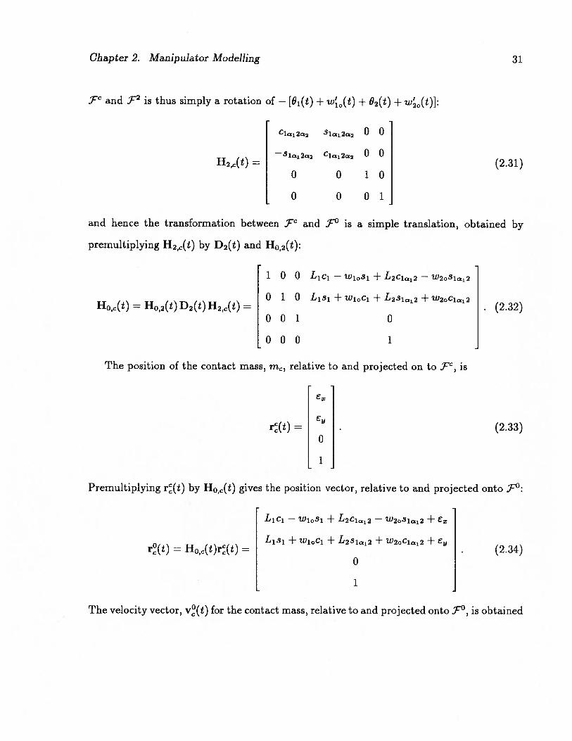
Chapter 2. Manipulator Modelling 31
fC and .F2 is thus simply a rotation of — [81(t) + w’0(t) + 82(t) +w0(L)]:
C1i2a2 81a12a2 0 0
H2(t)= 81cj22 C1a12a2 0 0
(2.31)o 0 10
0 0 01
and hence the transformation between FC and F° is a simple translation, obtained by
premultiplying H2,(t) by D2(t) and Ho,2(t):
1 0 0 L1c1 — w10s1 +L2C1a12 W2oSlai2
0 1 0 L1s1 + w10c1 + L2s112 + w20c1a12H0,2(t)D2(t)H2,(t) = . (2.32)
001 0
000 1
The position of the contact mass, m, relative to and projected on to F’, is
= U(2.33)
0
1
Premultiplying r(t) by H0,(t) gives the position vector, relative to and projected onto LF°:
L1c1 — w10s1 + L2C1a12—
W2081a12+ E2
L1s1 + wiOc + L281a12+ W20C112 + Eyr(t) = Ho,(t)r(t) = . (2.34)
0
1
The velocity vector, v(t) for the contact mass, relative to and projected onto F°, is obtained

Chapter 2. Manipulator Modelling 32
by differentiating r(t) with respect to t:
— (Lisi + w10c1)Oi —— (L2s1a12 + wloclaj2) + +
W2o81ai2 + E
v(t) = r(t)= (Lici — w10s1)01 +i10c1 + (L2C1a12 — WioSiai2)(é1 + Wio + 02)
+‘th2oClcxi2 + y
0
0
(2.35)
The position vector r(t) and velocity vector v(t) are used to derive the kinetic en
ergy, potential energy and dissipation function expressions for the contact dynamics in
section 2.4.
2.4 Derivation of Equations of Motion
Given the position and velocity vectors for the elemental link masses and the the contact
region mass (derived in section 2.3), the equations of motion for the manipulator and envi
ronment system are derived using the well known energy method of Lagrangian dynamics.
As noted in section 2.2 this approach to the derivation of equations of motion for robotic
manipulators is widely used [23,31,48,60]. It has the advantage that the resulting equations
are in a form well suited to numerical integration for the purposes of simulation studies.
Also, in the case of structurally flexible manipulators, the problem of accounting for the
movement of the centres of mass of the bodies as they deform is avoided. The structure of
the resulting equations of motion gives clear insight into the interaction of the rigid body,
structural and contact dynamics.
During the early stages of the research the equations of motion for several simple con
figurations of the manipulator and environment system, such as a single flexible link with

Chapter 2. Manipulator Modelling 33
unidirectional contact, were derived manually [22]. The equations for the two flexible link
system, presented below, were derived with the assistance of the Maple V algebraic com
putation system [67]. Maple V proved invaluable in helping to avoid transcription and
other mechanical errors which often arise in the course of manual algebraic manipulations.
Furthermore, Maple V includes a rudimentary FORTRAN code generator, which was used
to translate (with minimal errors) the equations of motion into source code which served
as starting points for the simulation subroutines which calculate the terms of the inertia
matrix and the right hand sides of the equations. As well, the J.TEX code generator in
Maple V was used to assist in the preparation of the equations of motion for typesetting in
this document.
The total kinetic energy, 7, of the system is
= 2 JMv dm1 +
1M2v dm2 + mcvT v, (2.36)
where Mk is the total mass of link k. The first two terms are the kinetic energies of the
links and the last term is the kinetic energy of the contact region. Expanding the vector
dot products in equation (2.36) and evaluating the integrals over the link masses (assuming
constant distributions of mass over the lengths of the links), the total kinetic energy is
rewritten as:
7- = Io1o+1Iiiiiioi
+ ‘21j (b +e)
+M2 (L + + [102+fl2]
(ô1 + + é2)2 + iitb
+I22j + [M2 (LiL2ci2i+ L2WloSai2&1 +L2c121o) + h12’2i
— (L1Sa12Ô1— + 10s2) I42i2i] (i + w10 + 62) +M2L18110

Chapter 2. Manipulator Modelling 34
+ (LiCai2i+ WloSal2ô+ai2io) 14221 + ( + é + + ti)
4m [(L + + (L + t4) (a1 + +
—m [(Lisi + wi0ci) Ô1 + (L2si12 + W2oClai2) (ô1 + W10 + 02)] x
+m [(Lici — w10s1)01 + (L2C1a12—w20s112)(1 + 11o + 02)]
—me, (tiii0si + W2o31a12) + m (zhi0ci + tb2ocIaj2) Ey
+m [— (L18a12— wlocaj2) w20Ô1 + (L2c12— W205a12)tub] (ô1 + W10 + 02)
+m [(LiL2ai2+L2Wioai2)01 + L2tui2o] (o1 + t140 + 02)
+m [(L1Ca12+ wbosai2)01tv20 + W10W20Ca12+L181tu10] . (2.37)
The assumption of constant mass distribution in the links is made for simplicity; any
mass distribution function, pk(xk), may be chosen and the integrals evaluated in closed
form or numerically, as necessary. The summations in equation (2.37) are the result of the
application of the method of assumed modes [41] to discretise the spatial variations of the
link motions. The upper limits of summation, k, are the number of admissible functions
included in the structural model of link k. The subscripted I factors are integrals of the
admissible functions. They are discussed in detail below, following the statement of the
system potential energy.
The link kinetic energy terms in equation (2.37) are in agreement with an appropriate
subset of the kinetic energy terms for a model of an orbitting space platform based mobile
flexible manipulator reported by Chan [681. Since the kinematic representation used by
Chan is markedly different from that described in section 2.3.1 the agreement of kinetic
energy expressions serves to validate the method used here.
The total potential energy, 1), of the system is
1) = — J gT r dm1— J gT r dm2
M1

Chapter 2. Manipulator Modelling 35
1 1 1 2+>T3ii’tb1+
2+k8(Lici — W1031 + L2C1a12 — W2oS1c2 — xw — E)
+k8(Ljsi + W10C1 + L231a12+ W2oClai2 Yw— )2
2 j. 2m
where g is the gravity field vector. The first two terms are the gravitational potential
energies of the links. They are followed by the elastic potential energies of the links due
to their structural stiffnesses. The last four terms are the elastic potential energies of the
contacting surfaces of the manipulator tip and the environment with the point of initial
contact located at xi + The zero condition for the springs used to represent the
contact stiffness is that of zero force.
The bk factors in equation (2.37) represent the rigid body components of the link
moments of inertia about the joint axis:
1 2‘ok = (Lk — Xk) dmk. (2.39)
J Mk
The other subscripted I factors in equations (2.37) and (2.38) represent integrals which
involve the set of admissible functions used as assumed modes to model the link structural
dynamics. Given a set of admissible functions, these integrals evaluate to constants in
the equations of motion. Employing the cantilever beam mode shape functions derived in
section 2.3.2 these integrals are evaluated, for mode i of link k, as follows:
‘iki= J (Lk
—
xk) qki(xk) dmk = 2-- (2.40)I3k
where 13k1 is the solution of the cantilever beam frequency equation (equation (2.22)) for
the ith mode of link k and pk is the mass per unit length of link k,
‘2ki= J k(Xk)2dmk = pkLk = Mk, (2.41)
Mk

Chapter 2. Manipulator Modelling 36
13ki
JLk
Elk(82)2
dxk = EIkLk MkWL, (2.42)
where Elk is the fiexural rigidity of link k in bending about its joint axis, and,
I pk (sinh/3k2Lk smI3kLk N‘4ki = 4’k(xk)dmk = 2— i (2.43)JMk /3kz \cosh/3kJk+cos/3k:LkJ
All of the I factors are retained as general constants in this derivation and in the subse
quent simulations to facilitate the use of any arbitrary set of admissible functions and link
dimensions.
Assuming that the energy dissipation in the system can be modelled using equivalent
viscous damping, the total dissipation function, R., for the system is
= +
1 2+ b12’4b1 +
[(Lisi + wi0ci)Ôi + (L2ia12 + W2oC1a12)(ê1 + o + 2)
+W10S1+ W2oSlai2 + J+b8 [(Lici — wi0s1)1+ (L2ci12 —w20s112)(o + w + 82)
+w10c1+ W20C2— Ej
1 1ezEx
where the subscripted b terms are equivalent viscous damping coefficients. The total dissi
pation function is somewhat analogous to the total potential energy function. The first two
terms represent the energy dissipated due to friction in the link joints. They are followed by
terms for losses in the links due to structural damping. The last four terms are the energy
dissipated in the materials of the contacting surfaces of the manipulator tip and the envi
ronment. The dissipation of energy in the links and the contact regions is due to hysterisis
associated with cyclic stressing of the materials. The selection of damping coefficient values

Chapter 2. Manipulator Modelling 37
is somewhat complicated by the fact that the energy dissipation is dependent on a number
of factors including temperature, stressing frequency and stress level. Lazan [69] provides
a collection of experimentally determined loss factors which are the ratio of the energy
dissipated per cycle to the maximum strain energy in the material. Assuming harmonic ex
citation these data can be used to estimate damping coefficient values of lumped parameter
systems following the method described by Meirovitch [70]. However, for more general situ
ations Gaylord and Gaylord [71] recommend that the damping in most structural members
be assumed to be a few percent of critical.
Using equations (2.37) and (2.38) to form the Lagrangian for the system, C’ T — 1), the
equations of motion are given by Lagrange’s equation, augmented with a disspation term:
d (ôL’ &C oR.o) = — —
+ Q (2.45)
where q is one of the system variables,
1, 02, ,i = 1,... ,ni}, ,j = 1,... ,n}, e,
selected as generalised coordinates and Q is the corresponding generalised force. The com
plete set of equations of motion consists of 4 + ni + n2 strongly coupled, nonlinear, second
order, ordinary differential equations. The general structure of each of the equations is
Q + bj + kT + g(q) + N(q, 4), (2.46)
where I = I(q) is a vector of inertia terms, j= j(t) is a vector of the second time derivatives
of the generalised coordinates (generalised accelerations), Q is a generalised force, b = b(q)
is a vector of dissipation coefficients,=
4(t) is a vector of the first time derivatives of
the generalised coordinates (generalised velocities), k = k(q) is a vector of stiffness terms
(which are generally weakly nonlinear functions of the generalised coordinates due to the
geometry of the system), q q(t) is a vector of the generalised coordinates, g(q) is the
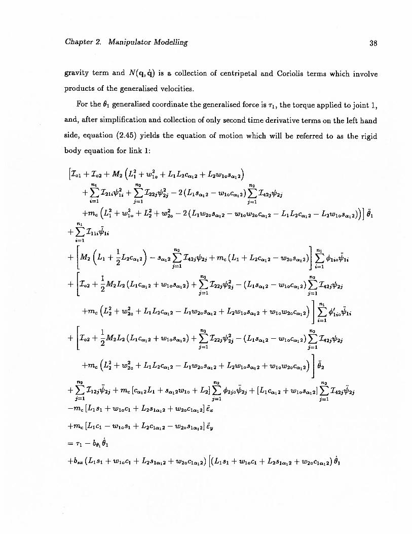
Chapter 2. Manipulator Modelling 38
gravity term and N(q, ) is a collection of centripetal and Coriolis terms which involve
products of the generalised velocities.
For the O generalised coordinate the generalised force is T1, the torque applied to joint 1,
and, after simplification and collection of only second time derivative terms on the left hand
side, equation (2.45) yields the equation of motion which will be referred to as the rigid
body equation for link 1:
[i + 102 + M2 (L + w0 +L1L2c12 +L2ioai2)
722
+I2iz”,b1j+I22i,b2— 2 (Liat2 — WioCaj2)142jI’2j
+m (L +w0+L + wo — 2 (LlW2oSai2 — WIOW20Ca12 L1L2Ca12 L2W10Sa12))j i
+ I11i11i
+ [M2 (L1 +L2c12)— I:: + m (L1 + L2c12
—2oSa2)] L
+ 1o2 + -M2L2(L1Ca12+ WloSai2) + 122jI’2j — (L18a12— wlocai2)
j=1 j=1
+m (L + w0 + LiL2ca12 — L1W2OSa22+ L2wlosai2 + W1OW2QCa12)]
+ [102 +M2L2(Lic12+W10Sa12)+I22j — (Lia12
+m (L + w0 +L1L2Ca12 —L1w20s12 + L2wlosaj2 + WloW2oCai2)] 02
+ + m [c12Li +s12w10 + L2] 2jo2j + [Liai2 + wlosa12] Ij/7
—m [Lisi + w10c1 + L2s112 + W2OC1a12]E
+m [Lici — wiosi +L2c1a12 — W2081a12]Ey
= T1 —
+b35 (L1s1 + W10C1 + L251a12+ W2oClai2) [(Lisi + w10c1 + L2Sai2 + W2oClai2) 6

Chapter 2. Manipulator Modelling 39
(L231a12+w20c12)62 — W10S1 —— (L2S1a12+w20c112)
— x]
—b3 (Lici — W10S1 + L2C1a12 — W2031a12) [(Lici — wiosi + L2C1a12 — W2081a12)8i
+ (L2C1a2 — W2OS1a12)62 + mc + tii2c112 + (L2c1a12— W2oSlai2) o— y]
+k (Lisi + W10C1 + L2S1a12 + W2oClai2) (Lici — wi0si +L2c112— W2081a12— —
e)
—k8 (Lci — w10s1 + L2c112— W2Q81a12)(Lisi + w10c1 + L2s1a12 + W2oC1ci2 Yw — E)
+gx (MiLsi + C1 + M2L1S1+ M2w10c1+ M2L2Siai2+
—gy (_M1L1c1— i I41j1j + M2L1c1 — M2w10s1+ M2L2Ciai2— 812 I42j2j
i=1 j=1
+ { [ML2(L13a12 — W1OCa12) + 2 (Lic12 + WloSai2) 142j’2j
+2mg (LiL2s12 +L1W20Ca12—L2w10c12 + WloW2oSai2)] 82
+1I2 [L2 (Lis12— W1OCa12)4c — (L28a12+ 2wi0)thi0j
2I21b11 — 2122 b2b2
+2 [(Llcai2 +w10s12)Wo — Cak2Wlo] ‘42j23 + 2 (L13a12— w10c12) ‘42j2j
—2mg [(w10 + L28a12 + W2OCa12)11)10 — (L1sa12 — W1OCa12 — w20)w20j
—2m0[(L1L2s12 + Liw2ocai2+ W1OW20Sa12— L2W10Ca12)11401} i+ [M2L2(L1Sa12 — wlocai2) + (L1ca12+ hl1o3ai2)I42j2j
+m0(L1L2Sa12+L1w20c12 +w10w20s2— L2ioCai2)]
+ [M2L2(Lisai2—
c12wi0)11i0_ + 2(Lisai2 —
+2 (L1Ca12+ 5ai2t’1o) lL I42j1’2j + 2m0 (L13a12 — W10Ca12— w20)12o
j=1

Chapter 2. Manipulator Modelling 40
+2m (LiL2ai2— wloL2caj2 + L1W2OCa12+w10w20s12)io] 2
+ [M2L2(Liai2 WloCai2)+(LlCai2+W1o3ai2)I42j2j
+m(L1L2s12 —w10L2c2+L1w20ca12 + WloW2oSai2)] Zi
+2 [(L1Sa12— wIocai2)I42j2j — I22j2j2j +2mc(Llsai2 — WloCai2 —w2o)b2o]
(2.47)
Similarly, for link 2 with the generalised coordinate 2 and the corresponding joint torque,
r2, the rigid body equation is:
[102 + M2L2(L1Ca12+w10s12)+ I22j’ — (L13a12—
+m (L + wL +L1L2c12 — L1W2oSa2 +L2W10Sa12+ WloW2oCal2)1 Oi
+ [M2L::ai2— + mc — Sa12W20)]
+ [102 + I22j + m (L
+ [102 + I22j + m (L + w0)] 2 + I12j2j +
—m [L2si12 +w20c112}ë + m [L2ci12 —w20si2]ë,
=r2—b0202
—b3 (L281a12+ W2øClai2) [(Lisi + W10C1 + L251a12+ w2oclai2) &1
+ (L251a12+ W2OCIa12)02 + +l0sl + i2os1ai2 + (L251a12+ W2oClai2)1140]
b8 (L2C1a12— W2051a12) [(Lici — wiosi + L2C1a12 — w2oslai2) &i
— (L2ci12 — w20s1a12)82 — é +(10c1 + th2oClai2 + (L2ci12 —w20s12)
+k8(L2s112 + w2ocIai2) (Lici — w10s1 + L2c1a12 W2o51cx12—

Chapter 2. Manipulator Modelling 41
—k3 (L2C1a12- w2oslai2) (Lisi + w10c1 +L2s112 + W2oCicj2 Yw —Ey)
1 fl2
+gx (M2L2sii2+ C1ai2I422) — gy (M2L2iai2— 81ai2I422)
+ [M2L2(WloCai2 — L1Sa12) — (L1ca12+ W1oSai2)I42j2j
—m (LjL2sai2+ Liw2ocaj2 WioL2Cai2+ wlow2oSai2)] è
— [M2L2ai2io+ 2Cai2ioI42j2j +
+2m [(L2Sa12+w20c12)io +w2olb2o]] 8
— + 2mcw2o2o](+ &). (248)
The time variation of the ith mode of the shape of link 1 is given by the generalised co
ordinate i& for which the corresponding generalised force is zero. Applying equation (2.45)
yields the deflection equation for link 1:
+ [M2 (L1 + L2Cai2)—
3ai21oI42j’2j + m(Li + L2ca12 — W208a12)]
+ [102 + M2L2(Lic12 + Wioa12)+ I22j — (Lis12 —
+m (L + wL +L1L2Ca12 — LlW2oSat2 +L2w10s2+ W1OW2OCa12)] io] i
+I21j1j + {M210 + (M2L2ci2 Sai2I42i)2)
+rnc [qizo + (L2Ca12— W203a12)14]} 412oh/’1z
+ { (M2L2Cai2—
Sai2I422i) 1io + (102 + I22))

Chapter 2. Manipulator Modelling 42
+m [(L2Ca12 —w20s12) + ( +)] }
+ { [cai: — 142j2j + m (L2ca12— 1112o3a12)] &jo
+ ‘o2 + 122ij + rn (L + w)] iQ} 2
fl2
-f-jo + cai2cliwI42b2+ [m1.(L2q10 + ca12qiio)]3=1 j=1 j=1
—rn [1n81 + (L2s1a12+ W2OC1a12)4cJ a, + rn [4i0ci + (+L2ciai2— w2081a12)1jo] E
= —b1J.1—
—b3(10s1 + L2S1a2j0+ W2oC1ai2j0)[(Lisi + wci + L251a12+ w2oclai2) 01
+ (w2oclai2 + L251a12)02 + e + W1o81 + W2031a12+ (L231a12+w20ci12)tb]
—b3(10c1 + L2C1aL2iO —w20s1120)[(Lici — W10S1 + L2C1a12 —w20s112)Ô1
+ (L2ci12— W2o31a12)02 — Ey + 1ol + W20C12 + (L2ci12 —w20s112)
+k8 + L2S1ai26jO + W2oC1ai294o) (Liei — wi0si + L2C1a12 W2o81a12— — e)
—k (410c1+ L2c1a12ç/4j0— W2oS1ai24j0)(Lisi + w10c1 + L2s112 + w20c1a12 — E)
+gxslI4li —
+ {1211 + [M2 (L2Sai2 + 10) + cai2 142j’2j + m (w10 + L2s12 +w20c12)] 1jO
— [M2L2(Llsai2 — W1QCa12) + (Llcai2 + l111o5ai2)I42i2i] io
—m(L1L2Sa12 +L1W20Ca12 —L2wiocai2+ WloW2oSai2)
+ { [M2L212 + 2c12 I42j2j + 2m (L2s12 +:12)]
1io02
+2 M2L2ai2ti4o + a2 I42j&2j + Cai2tL4o I42jlI’2j:1=1 j=1

Chapter 2. Manipulator Modelling 43
+m (Sai22o + (L2sai2 + w2ocaj2)
2[f2L2ai2io+ I22j2j2 + Cai2WloI42j)2j
+m(w20b20+ (L2Sa12+ W2ocai2)1o)] io}
+ [M2L2ai2+ Cai2I42j2j+ mc(L23a12+ W2ocai2)]
+2 { [M2L2Sai2toiio + Sai2I42j2j+ Cai2W1oI42jJ2j
+mc(L2sai2o+w2oC12W10+ 1jo — + mcw2oti2o) io} 82
+ [M2L2Sai2+ Ca12 ‘42j2j + m (L2Sa12+ W2oCai2)) 1jo
+2 [(Sai2I422 + mcsai2zi2o) iio — + mcw2oui2o) io] to (2.49)
Likewise, the deflection equation from the jth mode of link 2 is obtained from (2.45) using
the generalised coordinate b2i:
[112j + (L1CaI2 + Sai2Wlo)142j + m (Lic12 + w10s12 + L2) 2jo1
+ [Cai2142 + mc1220] &jo1i + [112j + mL22501 oij
+[112j + mL220j82 + ‘22j2j + m20 2jo2j — +mc2joclai2ëv
= —b2/’2—
b8x2joS1ai2 [(Lisi + wioci +L2s112 +w20ci12)8 + (L2s12 +w20ci12)82
+6rW1o81 + W2051cz12+ (L251cz12+ w2oc1a12)i4o}
bsy2joC1a2 [(Lici — ws1 + L2c1a12— w2oslai2) Oi + (L2Ca12 W2o51a12)82
6!,W1OC1+ W2oClcxi2 + (L2C1a12 W2o51a12)th0J

Chapter 2. Manipulator Modelling 44
+ksx42joS1ai2 (Lici — w10s1 +L2c112 ——
—
—ksyq52jociai2(Lisi + WioC + L2S1a12+ W2oClai2— Yw — e1)
+gs1aj2I42j— 9yC1ai2142j
+ [I22j’2j — (L18a12— tUloCai2)142j + m (wlocai2 — L1Sa12 + w20)q52jo] 0
+2 {I22&2 + mw2o20102— ai2142j1o + I22b2iW0— m (sa12thio — w20t140)b20}i
+[122j’c/-’2j + mcw2oq2jo] (th, + & + 2i4o02) (2.50)
The generalised coordinate for the x direction component (in the world frame) of the
contact mass deflection is e and the x direction contact equation is:
—m [Lisi + L2S1a12+ W10C1 + W2C112]01 — ms1 1jo1j
—m [L2s112 + w20c1a12] —m [L231a12+ W2OC1a12I02
—ms112 2jo2j + mE
bexx — kexEx
—b [(Lisi + wioc1 + L2S1a12+ W2OC1a12)Oi + (L231a12+ w20c1a12)02
+E + W10S1 + W2oSlcxi2 + (W2oClai2 + L281a12)ti4ol
+ksx (L1c1 — w10s1 + L2c1a12—— — Ex)
+m (Lici — w10s1 + L2c1a12 W2031a12)0 + m(L2ci12— W2051a12)02
+m(L2ci12 —w20s112)tb + 2m?i20c112?d40
+2m {(L2c112— W2051a12)02 + 10c1 + zb20c12 + (L2ci12
— w2031a12)4] ôi
+2m [(L2cm12 — W2081a12)l)1o + W2oC1ci2j 02. (2.51)
Finally, the y direction contact equation, obtained with the generalised coordinate es,, is:
ii [Lici — w10s1 + L2c1a12 W2o31a121 1 + mc1 1jo1i

Chapter 2. Manipulator Modelling 45
+m [L2C1a12— W2o31a12] — m [L2Clai2 — W2oSi2]02
+mc112 2jo2 + mE
= beyEy — keyEy
+b [(Lici — w10s1 +L2c112 — W2QS1a2) Si + (L2ci12 —w20s112)02
+ iJ-10c1 + w20c1a12+ (L2c1a12—w20s112)Wi0]
+k3 (Lisi + wi0ci +L2s112 + W2oCiaj2— Yw c11)
+m (Lisi +L2s112 + w10c1 + w2oclai2) 0 + m (L251a12+ w2ociai2) 02
+m (L231a12+ W2oClai2) ti4 + 2mctb2osiai2ti4o
+2mg [(L251a12+ lD2oC1ai2) 02 + WioSi + W2oS112+ (L251a12+ W2oCiai2) oj 6
+2m [(L281a12+ W2oClai2) Wlo + W2oSlai2] 62. (2.52)
Several steps have been taken in an effort to ensure the correctness of the derivation of
equations (2.47) through (2.52). As noted previously, the kinetic energy expression (equa
tion (2.37)), from which most of the terms in the equations of motion arise, is in agreement
with that derived independently by Chan [68]. Furthermore, Chan’s derivation is in agree
ment with two other independent derivations for related systems carried out by Mah [35]
and Ng [72]. The application of Lagrange’s equation to the energy expressions to obtain
the equations of motion and the subsequent simplification and manipulation of those equa
tions was done using the Maple V algebraic computation program. This method protects
against errors which are common in manual algebraic manipulation such as transcription
errors, sign errors and misapplication of the chain rule of differentiation. Finally, as will
be discussed in section 4.5, the FORTRAN coded form of the equations of motion have been
validated against the code developed by Mah [35] both by comparison of calculated values

Chapter 2 Manipulator Modelling 46
for the terms in the inertia matrix and on the right hand side, and by comparison of ho
mogeneous responses for a variety of initial conditions. Mah’s program has been similarly
validated against programs developed independently by Chan [681 and Ng [72].
With reference to the generic equation of motion, (2.46), it is evident that, when contact
exists, equations (2.47) through (2.52) describe a system of 4 + ni + n2 damped, coupled,
nonlinear oscillators. The oscillators are forced by the joint torques in the rigid body
equations which act to change the joint angle generalised coordinates.
The coupling among the oscillators ensures that an excitation of any of the generalised
coordinates will be transmitted to all of the other generalised coordinates. The inertial
component of the coupling is evident in the fact that the inertia terms on the left hand side
of each equation are a weighted sum of all of the generalised accelerations. Considering the
complete set of equations, the weighting terms can be written as a symmetric generalised
inertia matrix. The terms in that matrix can be divided into two groups; those which are
inherent in the dynamics of a serially connected chain of flexible links and those which
arise due to the existence of contact between the manipulator tip and an environment
surface. The same division is true of the nonlinear right hand side terms, N(q, 4), which
are functions of the generalised coordinates and velocities. On the other hand the coupling
in the dissipation and stiffness terms on the right hand side exists solely due to contact.
As will be shown in section 2.5, the contact force exerted by the manipulator on the
environment can be expressed as a function of the generalised coordinates. Thus, joint
torque inputs will tend to excite oscillations of the generalised coordinates which will be
expressed as oscillations of the contact force. The goal of force control is to calculate and
apply joint torques which will cause the contact force to quickly follow changes in the desired
contact force level.
In the absence of contact the system becomes a set of ni +n2 damped, coupled, nonlinear
oscillators with an additional two rotational degrees of freedom. The joint torques act to
Chapter 2. Manipulator Modelling 47
produce rotations of the link bodies about the joints and the inertial and nonlinear cou
pling ensures that oscillations of the generalised coordinates associated with the structural
dynamics are excited.
Equations (2.47) through (2.52) can be transformed to the equations of motion for
several other configurations which have been investigated in the course of the research.
Setting each element of the set of coefficients {m, bex, b3, b3, kex, k3, k8} to
zero and dropping the generalised coordinates E and ey and equations (2.51) and (2.52)
yields the 2 + ni + n2 equations of motion for a planar two link flexible manipulator in free
motion. The resulting equations are shown in section A.l of Appendix A. These equations
govern the motion of the manipulator when it is not in contact with the environment.
Note that by dropping the generalised coordinates and e in the absence of contact, the
motions after contact of the contacting surfaces are neglected. By implication, when contact
is broken, the contacting surfaces effectively come immediately to rest without residual
deflection. This assumption is reasonable considering that the masses and deflections of the
contacting surfaces are small and that neither plastic deformation of the surfaces nor gross
motions of the environment are included in the model.
Starting from equations (2.47) through (2.52), the equations of motion for a planar
two link manipulator with rigid links contacting a deformable environment are obtained
by setting each of the coefficients {I1k, ‘2ki, JJ3ki, ‘4ki, bk, i 1,. . . , rik, k 1, 2} to zero,
dropping the generalised sets of coordinates {‘,bi2,i 1,... ,m1} and {b23,j = 1,... ,n2} and
dropping equations (2.49) and (2.50). The resulting four equations of motion are shown
in section A.2. Further operation on this resulting set of equations, namely setting each
of the coefficients {m, bex, bey, b3, kex, key, k8x, ksy} to zero, dropping the generalised
coordinates e,, and E and dropping equations (A.7) and (A.8) yields the two equations of
motion for a planar, rigid, two link manipulator in free motion, shown in section A.3.

Chapter 2. Manipulator Modelling 48
Finally, the 2 + n1 equations of motion for a single flexible link in contact (section A.4)
and the 1 + n1 for the same link in free motion (section A.5) are arrived at by setting
the coefficients {IO2,I12,I22,I32,I42, b2, b€, b3, kex, k3,i = 1,... ,n2} to zero, dropping
the generalised coordinates 62, {b2,i = 1,. . . ,n2} and e, and dispensing with equations
(2.48), (2.50) and (2.51) in the former case and by additionally setting the coefficients
{m, key, k3} to zero, dropping the generalised coordinate e, and dispensing with
equation (A.13) in the latter.
2.5 Contact Force Model
Figure 2.5 shows the geometry of the two flexible link manipulator and deformable environ
ment system with the link deflections and the environment model much exaggerated in scale
(compared to Figure 2.1). The contact force arises from the local compression of the regions
surrounding the point of contact between the link (or end-effector) tip and the environment
surfaces. The local dynamics of the contacting surfaces are represented, as recommended
by Johnson [62], by a contact region mass on a damped, linearly elastic foundation for each
surface. The deflection of the combined contact mass from its location at the instant when
contact is made represents the local compression of the surfaces. Note that, while the local
compression of the manipulator tip surface in general has a component along the axis of the
last link, the links are assumed to be stiff in that direction and the effects of global axial
compression of the links are ignored.
The expressions for the contact force components as a function of the generalised coor
dinates of the model will now be derived by considering the geometry of the system and
the forces acting on the contact region masses. These expressions are necessary to the sim
ulation studies in order to permit the contact force between the link tip and environment

Chapter 2. Manipulator Modelling 49
y€
I
x
Figure 2.5: Manipulator—environment model geometry for derivation of contact force expressions.
Ijkev
sym= m+ me
yw
b5
xw ox

Chapter 2. Manipulator Modelling
mpc
50
k5(e— ô—x)
b5(—x1)
kex(E ô X)
bex’x
b5(— *tp)
(a) Total contact mass
Figure 2.6: Free body diagrams for the x direction contact region mass.
surface masses to be calculated from the results of the integration of the equations of mo
tion. Furthermore, they are used, in simplified form, to devise the initial controller model
coefficients for the force control algorithm in Chapter 5.
Based on the free body diagram shown in Figure 2.6a a force balance for the total contact
mass, m = m3 + me, in the x direction yields
më = —k9 (e1, — —— ( — Sx
— w) — b3 (r — — bexE. (2.53)
Considering each of the surfaces separately, with the x direction contact force, F, acting
equally but in opposite directions on each contact mass as shown in the free body diagrams,
k5 (E— — xtjp
F F
(b) Manipulator tip contact mass
kex(Eôx)<w)
b ex
(c) Environment contact mass

Chapter 2. Manipulator Modelling 51
a force balance on m3 (Figure 2.5b) gives
— F — k3 (e — — x) — b3 ( — = m3 (2.54)
and a force balance on me (Figure 2.5c) gives
F — kex (e — — x)— = meêYx. (2.55)
Solving equation (2.53) for ë and substituting the results into equation (2.55), noting that
=— 8x —
x, yields:
F = (kexx+ bexx)+ x.. x)j. (2.56)
A similar procedure applied in the y direction yields the expression for that component of
the contact force, F:
= (keyEy + beyy) + [ksy (Ytip — Yw — e) + b (th —ay)]. (2.57)
‘rn
Expressions for the world frame manipulator tip position (x2 and y) and velocity (i1
and !‘tip) components which appear in equations (2.56) and (2.57) were derived as part of
the kinematic analysis in section 2.3 (equations (2.34) and (2.35)).
When the tip of the manipulator is just contacting (but exerting no force on) the en
vironment the following geometric relationship exists among the link lengths, joint angles
and the location of the environment:
= L1 cos i9 + L2 cos ( + 8) = L1c + L2c2
and Yw = L1 5111 8 + L2 sin (8’ + 6) = L1s + L2s2, (2.58)
where O and O are the particular values of the joint angles at which contact occurs.

Chapter 2. Manipulator Modelling 52
2.5.1 Hertz Contact Model
The values of the contact region masses, m5 and me, stiffnesses, kex, key, and k5, and
damping coefficients, bex, bey, b3 and b3, in this lumped parameter contact model must be
related in some way to the material properties of the surfaces in contact. For instance, an
aluminium end-effector in contact with a steel assembly jig will have much higher stiffness
values and lower mass values than a rubber cover tool contacting a wooden surface. The
solution for the deformation of contacting spherical surfaces, derived in 1882 by Hertz,
provides some insight into selecting contact mass and stiffness values based on the physical
properties of the materials in contact. It must be noted that the Hertz theory is based on
the assumptions that the contact occurs between surfaces of non-conforming shape and is
quasi-static. As a result, it can only be used as a guide in the selection of coefficient values
for the more complex, dynamic contact case being modelled here.
One result of Hertz’s analysis is that the decrease in distance, 8, between the centres of
two spheres held in contact by a force F is [63]
2 1 1 1_v2 1—vaS = F3 {D2 ( + where D 1
+ 2 (2.59)
is the inverse of the effective planar strain modulus of the materials, v1 and v2 are the
Poisson’s ratios of the materials, E1 and E2 are the moduli of elasticity and R1 and R2
are the radii of curvature of the spheres. Equation (2.59) can easily be expressed as a
force/compression relationship:
F = KS, (2.60)
where(R8) R1R2
K= and R=D
In this expression R is the effective radius of curvature, that is, the contact between surfaces

Chapter 2. Manipulator Modelling 53
of curvature R1 and R2 is equivalent the contact between a surface of curvature R and a
flat surface [64].
Note that, unlike in Hooke’s Law for a linear spring, the stiffness in equation (2.60) is a
function of the square root of the compression, that is, the stiffness of the material increases
the more it is compressed. Given the restrictive assumptions under which equation (2.59)
was derived and the fact that in elastic contacts between hard materials the surface deflec
tions must be small, the contact stiffness coefficient values used in the present research were
obtained by approximating equation (2.60) by its tangent at an appropriate nominal level
of contact force. Details of the calculation of the coefficients for specific combinations of
materials are included in Chapter 5.
It follows from the Hertz theory [63] that the area of contact between spherical surfaces
is a circle of radius
a (FDR). (2.61)
On the basis of this, a first order estimate of the volumes of material moved by the defor
mation of the surfaces is that they are equal to the segments of a sphere of radius R and
heights S and 62, that is,
= 7rS (R— -6) and V2 7r6 (R — s2) . (2.62)
The deflections of the individual surfaces, 6 and 62, sum to the total deflection given by
equation (2.59) and are in inverse proportion to the planar strain moduli of the surface
materials. These volumes, combined with the densities of the contacting materials, give
the mass of material on each surface that is involved in the contact deformation and thus
provide a basis for the selection of values for the contact region masses, m5 and me.

Chapter 2. Manipulator Modelling 54
2.6 Voltage Controlled DC Electric Motor Actuator Model
In large, flexible manipulator systems such as the Space Shuttle Remote Manipulator Sys
tem (SSRMS), or Canadarm, and the proposed Mobile Servicing System (MSS) and Special
Purpose Dextrous Manipulator (SPDM) for the Space Station Freedom, the links are driven
by direct current electric motors at each joint. A typical DC motor actuator system, con
trolled by armature voltage, consists of:
• a signal amplifier which raises the control input voltage signal to a level suitable to
drive the motor armature;
• a current amplifier which produces the current through the motor armature;
• the motor itself with its inherent armature resistance and inductance, rotor inertia
and mechanical as well as electrical damping; and
• a gear box which raises the motor torque to the level required to drive the link.
Figure 2.7a shows a block diagram of such a typical DC motor actuator system.
The mathematical model of an armature voltage controlled DC motor is as follows [65j.
With reference to the armature circuit diagram in Figure 2.7b, the sum of voltage drops
around the armature circuit is:
Va = Raja + Laja + Vb, (2.63)
where Va is the armature voltage, derived from the control input signal, Ra is the electrical
resistance of the armature windings, a is the current through the armature windings and
La is the inductance of the windings. The back emf, vb, a feedback voltage proportional to
the armature speed, 0a, is a result of the rotation of the motor armature in the magnetic
field induced in the stator windings;
Vb KemfOa, (2.64)

Chapter 2. Manipulator Modelling 55
(b) Armature circuit
Figure 2.7: Schematic of direct current motor actuator system.
(a) Block diagram
+

Chapter 2. Manipulator Modelling 56
where Ke is the back emf coefficient. Equation (2.63) can be rewritten as an ordinary dif
ferential equation for the armature current in terms of the motor parameters, the armature
speed and the applied armature voltage, the latter being the forcing function:
Laja + Raja Va — Ke,6a. (2.65)
Equation (2.65) constitutes the electrical model of the motor. Mechanically, the motor
is represented by an armature inertia, ‘a a frictional damping, ba, proportional to the
armature speed, and the load torque, TL, at the motor side of the gear box. A torque
balance for the motor yields:
1aa Tm — TL — baOa.
The torque produced by the motor, Tm, iS proportional to the current in the armature
windings, or
Tm = Kra, (2.66)
where K.,. is the motor torque coefficient. Thus, the mechanical model of the motor as
viewed from the motor side of the gear box is
TL = K.rja — Ia&a — baa. (2.67)
The gear box increases the torque by a factor Ng, the gear ratio, at the expense of decreasing
the shaft speed by the same factor such that
= N9TL and = jIa.
Thus, when viewed from the link side of the gear box at joint k the mechanical equation of
the motor is
Tk N9Krja — Ng2 (2ak + bask) . (2.68)
This actuator model is coupled to the rigid body equation of motion for the link being
driven by adding the inertia, NIaOk, and damping, Nba8k, terms from equation (2.68)

Chapter 2. Manipulator Modelling 57
to the corresponding terms in the rigid body equation and by using the geared up motor
torque, NgKTia, as the joint torque, Tk. In order to calculate this joint torque the differential
equation for the armature current (2.65) must be solved simultaneously with the equations
of motion since it involves the armature speed which is proportional to the joint rate.
Section A.7 shows an example of how the coupling is implemented for the equations of
motion for a single flexible link in free motion driven by a DC motor.
This linear model of an armature voltage controlled DC motor actuator is widely used
and accepted [65]. The signal and current amplifiers are components of such an actuator
system that are often overlooked in modelling. They are important not only in that they
are part of physical actuator systems but also because they are the source of the dominate
nonlinear feature of the actuator system, saturation. The voltage drop which can be applied
across the motor armature is limited as is the current which the motor may draw. Figure 2.7a
shows the amplifiers as linear devices with limits and they are modelled in the TWOFLEX code
in much the same way; if the calculated values of voltage or current exceed the saturation
limits the values are clamped at the limits. The actuator model neglects features of the
motor dynamics such as non-viscous friction and torsional flexibility in the shaft and gear
head. These features are ignored in order to focus on the control issues which arise due to
the structural dynamics of the manipulator links.
Section 5.6 presents results of several simulations of maneuvers of a prototype Space
Station Mobile Servicing System (MSS) arm modelled as a two flexible link manipulator
with DC motor actuation.

Chapter 2. Manipulator Modelling 58
2.7 Summary
This chapter has presented the derivation of models for the kinematics and dynamics of
a planar two link manipulator with flexible links making contact with a deformable en
vironment. Also derived are expressions which relate the contact force to the generalised
coordinates of the dynamics model and relationships between the physical properties of the
materials in contact and the parameters of the contact dynamics model. The derivation
of the contact dynamics model is the primary contribution of the chapter in that, unlike
the models used in previously published robotic force control research, the model includes
the effects of inertia and damping in the local region surrounding the point of contact, in
addition to the contact stiffness. Results from the theory of elasticity, based on the work of
Hertz, indicate that the linear contact dynamics model used here is an approximation to the
more complex situation in which the contact stiffness and the mass of the region deflected
during contact vary nonlinearly with the contact force. However, the Hertz model is also
limited by its tacit assumptions of non-conforming surface shapes and quasi-static contact.

Chapter 3
Control Algorithm
3.1 Introduction
This chapter presents derivations and discussions of the various parts of the overall force
control strategy that is the focus of the research. At the heart of the control strategy is a
multivariable, receding horizon, adaptive, long range predictive control algorithm. Devel
oped with the primary goal of providing stable, accurate tracking control of desired levels
of contact forces between the manipulator tip and its environment, the algorithm can also
be used to control the gross motions of the manipulator when it is not in contact.
In the early stages of the research several controller designs were investigated before long
range predictive control was selected. The complexity of the nonlinear, coupled dynamics
of a flexible manipulator and environment system make conventional PID controller and
compensator designs impractical. Some of the difficulties with conventional designs can be
overcome with the use of gain scheduling but to do so requires very complete knowledge
of the plant dynamics over the operating range, including the time scales of characteristics
which are likely to necessitate gain changes. State feedback techniques are better suited
to complex dynamic systems. A pole placement tracking controller was designed for force
control of a single flexible link and was successful with the significant exception of its
inability to remove steady-state errors from the response. A similar deficiency was found to
limit the use of linear quadratic optimal state feedback. A scheme to use an adaptive inverse
59

Chapter 3. Control Algorithm 60
dynamics model of the system to provide state feedforward for the removal of steady-state
offsets was devised but the robustness of such a scheme is questionable.
The long range predictive control design that is developed in this chapter has the ad
vantage of possessing inherent integral action to yield a steady-state error free response.
Setpoint tracking is included directly in the formulation, the resulting control law is op
timal in the sense of minimising the sum of squares of the difference between the future
setpoint levels and the predicted output levels, and the algorithm is easily implemented in
an adaptive, digital controller form. Predictive control is well suited to deal with systems
exhibiting an abundance of lightly damped modes and non-minimum phase characteristics
as is the case in flexible manipulator force control. The inclusion of the expected future
effects of these characteristics in the controller cost function results in a control law which
produces more effective compensation than one based solely on instantaneous sensor data.
The Generalized Predictive Control (GPC) algorithm of Clarke, et al. [29] incorporates
many of the beneficial features of earlier predictive algorithms. It is a relatively mature im
plementation of the concepts of predictive control which has sparked a great deal of interest
and ongoing study of its properties and potential applications.
The dynamics of a flexible link manipulator in contact with deformable environment
present several challenges to the design of a force control algorithm. The dynamic behaviour
is highly coupled, nonlinear, stiff, discontinuous, and nonminimum phase. To deal with the
strong coupling, the predictive controller design is based on a multivariable model that
includes all of the open ioop system modes and their interactions. Nonlinearities arising
from the system dynamics are dealt with by making the controller adaptive, that is, an
instantaneous linear model of the system is used and the coefficients of the model are
updated regularly, on-line, to reflect the changes in the system due to its nonlinear nature.
The open loop system is, in most configurations of practical importance, stiff, in both
physical and mathematical senses. The natural frequencies of the open loop modes can easily

Chapter 3. Control Algorithm 61
span a range of several orders of magnitude in the case of a highly flexible manipulator in
contact with a metallic surface. This characteristic of the system causes difficulties in the
numerical integration of the equations of motion, as will be discussed in Chapter 4. It also
leads to the coefficients of the instantaneous linear model, on which the controller is based,
being sensitive to small changes in the system configuration. As in the case of nonlinearities,
this difficulty is overcome by using an adaptive control approach.
Contact force control is a discontinuous problem due to the fact that the contact force
can, by definition, only take on either positive or negative values (depending on the orien
tation of the reference frame in which it is measured). When the manipulator tip looses
contact with the environment surface the contact force is zero and the error signal available
to the controller is independent of the manipulator state. While it is possible that, even
with such a degenerate error signal, the controller will successfully return the manipulator
tip to the environment surface and continue stable control of the contact force, it is more
likely that the system will become unstable with manipulator tip repeatedly bouncing on
and off the surface. To avoid this situation the controller is designed to switch from a force
control mode to a motion control mode when the contact is unexpectedly broken. The
objective of the controller is then to return the manipulator tip to the surface and switch
back to force control mode. The switching of modes between force and motion control is
governed by a contact control logic block at a level above the force and motion controllers in
the manipulator control hierarchy. Two operational strategies for the contact control logic
are discussed and demonstrated in Chapter 5.
The structural flexibility of the manipulator links makes the contact force response of
the system nonminimum phase. Physically, a nonminimum phase system is one for which a
positive step input produces a response which is initially negative and subsequently reverses
sign. In free motion, the tip of a flexible link subjected to a step torque input oscillates about
the path that would be described by the tip if the link were rigid. Due to the inertia of the

Chapter 3. Control Algorithm 62
link, the tip initially lags and the oscillation is initially negative. This characteristic carries
over into the contact force response when the link is acting on a surface. Mathematically, a
nonminimum phase system is characterised by the presence of unstable zeros in the transfer
function numerator. Predictive control is well suited to dealing with nonminimum phase
systems because the prediction horizon can be extended to include the nonminimum phase
portion of the response and it can thus be compensated for in the calculation of the control
inputs.
Section 3.2 presents a review of the single input, single output (SISO), Generalised Pre
dictive Control (GPC) algorithm of Clarke, et al. [29,32], a discussion of the control law
structure and a derivation of the closed ioop system characteristics. The development of
a multivariable predictive control algorithm based on GPC is presented in section 3.3. A
new extension of the algorithm with a static equilibrium bias term that takes advantage of
available a priori knowledge of the dynamics of force controlled manipulators is presented in
section 3.4. This extension is an original contribution of this thesis. The parameters of the
predictive control algorithm and their effects on the shaping of the closed ioop response are
discussed in section 3.5. A discussion of parameter estimation, focussing on the Exponential
Forgetting and Resetting Algorithm (EFRA) is presented in section 3.6, and a description
of the structure and logic of the complete adaptive multivariable force/motion controller in
section 3.7. The chapter concludes with a discussion of stability and convergence charac
teristics of the adaptive, predictive control algorithm (section 3.8).
3.2 Review of SISO GPC Algorithm
This section briefly reviews a nonadaptive, single input, single output (SISO) long range
predictive control algorithm, known as the Generalized Predictive Control (GPC) algorithm,
developed by Clarke, et al. [29,32]. This discrete time algorithm yields a control law with

Chapter 3. Control Algorithm 63
inherent integral action and robustness to inaccuracies in both model order and time delay.
The algorithm is based on prediction of the plant output for a series of future time steps.
The predictions are expressed in a form which allows a solution for an optimal (in the sense
of minimisation of a quadratic cost function) set of future control inputs that will minimise
the error between the predicted plant output and the desired setpoint. This procedure is
conducted in a receding horizon context, that is, a new set of control inputs are calculated
at each time step and only the first member of the set is used. Receding horizon predictive
control predates GPC in the process control literature but, as the name suggests, the GPC
algorithm is a generalised form of the method. Indeed, it has been shown that, depending
on the choice of parameters, the GPC algorithm results in control laws identical to a variety
of well known algorithms [73—75].
The plant to be controlled is modelled in the discrete time domain by an input/output
representation of the form
A(q’)y(t) = B(q’)u(t — 1) + , (3.1)
where A(q’) and B(q1)are polynomials, of degree na and nb respectively, in the backward
shift operator q’:
A(q1) = 1 +a1q’ +a2q2 + . .. + anaq,
B(q1) = b0 + b1q’ + b2q2 + ... +
where q1x(t) = x(t — 1),
y(t) is the time series of plant output values and the plant input time series is u(t). The
last term in equation (3.1) is a disturbance term consisting of (t), an uncorrelated ran
dom sequence and L 1— q’, the differencing operator. This model assumes that the
disturbances to which the plant is subject can be modelled as steps of random magnitude

Chapter 3. Control Algorithm 64
occurring at random times [76]. Using the Diophantine identity [77],
1 = E(q1)A(q’)z + qF(q’), (3.2)
the plant model can be manipulated to yield a j—step ahead predictor of the plant output:
y(t + j) = Fj(q’)y(t) +E(q1)B(q1)L\u(t + j — 1) + E(q1)(t + j). (3.3)
The polynomials E3(q’) and F3(q1)in equation (3.2) are completely defined given A(q’)
and j, and are unique provided that [78]:
deg(E,) j and deg(F,) <deg(A).
The coefficients of E+1 and F3+1 are calculated from E, and F, with minimal computational
effort using simple recursion formulae [29]. The predicted output y(t + j) is the sum of
filtered time series of the output, the input and the disturbances. Given the fact that the
degree of E3 is, at most, j — 1 and the assumed random nature of (t), the contribution
to y(t + j) of the disturbance sequence is not only unknown but unknowable. Hence, the
optimal predictor of y(t + j) given the information available at time step t is
(t + jt) = F,y(t) + Gu(t + j — 1), (3.4)
where G3= E3B = gjo+gjlq1+...+gj(nb+j_flq(flb+I 1)• The optimal prediction (t+j It)
can be written as a term, f(t + j), which consists entirely of past inputs and outputs (in
effect, the free response of the system) summed with terms due to the future control input
increments which are yet to be determined.
Defining N2 as the prediction horizon and considering predictions at each of the next
N2 steps into the future the following vectors are formed:
= + 1 t) (t +2 It) ... (t + N2It)]:
(3.5)
[ut u(t + 1) ... u(t + N2 — 1)] , and (3.6)
r = [f(t+1) f(t+2) ... f(t+N2)]T,
(3.7)

Chapter 3. Control Algorithm 65
where
f(t + 1) = Fi(q’)y(t) + (Gi(q’) gb) Au(t)
f(t + 2) F2(q1)y(t) + q (G2(q’) g2lq — g2o) Au(t)
f(t + N2) = FN2(q’)y(t) + qN2 (GN2(q’)— gN2(N2-1)q’ — ... — gN2o) 1u(t).
(3.8)
The set of N2 prediction equations of the form of equation (3.4) are written in matrix form
as
5’ = G’ü + f, (3.9)
where G’ is an N2 x N2 lower triangular matrix whose elements are the coefficients of the G3
polynomials from equation (3.4) corresponding to the yet to be determined future inputs.
A quadratic cost function, J1, is defined:
J1 = (5’_w)P(5’_w)+AuTu
= (3.10)
The vector
[wt + 1) w(t + 2) ... w(t + N2) (3.11)
is a sequence of future setpoints, hence, the first term of this cost function is simply the sum
of squares of the errors between the predicted plant output and the desired setpoint at each
of the next N2 steps into the future. The second term is the sum of squares of the future
control input increments (i.e., the incremental control energy), weighted by a constant, ).
Minimising J1 with no constraints on future inputs yields the control law
u = (c’’ + AI)’ G1T(w— f) (3.12)
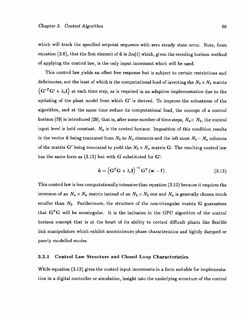
Chapter 3. Control Algorithm 66
which will track the specified setpoint sequence with zero steady state error. Note, from
equation (3.6), that the first element of ii is Liu(t) which, given the receding horizon method
of applying the control law, is the only input increment which will be used.
This control law yields an offset free response but is subject to certain restrictions and
deficiencies, not the least of which is the computational load of inverting the N2 x N2 matrix
(G’ TGI + at each time step, as is required in an adaptive implementation due to the
updating of the plant model from which G’ is derived. To improve the robustness of the
algorithm, and at the same time reduce its computational load, the concept of a control
horizon [79] is introduced [29]; that is, after some number of time steps, N< N2, the control
input level is held constant. N is the control horizon. Imposition of this condition results
in the vector ii being truncated from N2 to N elements and the left most N2 — N columns
of the matrix G’ being truncated to yield the N2 x N matrix G. The resulting control law
has the same form as (3.12) but with G substituted for G’:
u (G’G + i)’ GT (w — f). (3.13)
This control law is less computationally intensive than equation (3.12) because it requires the
inversion of an N x N matrix instead of an N2 x N2 one and N is generally chosen much
smaller than N2. Furthermore, the structure of the non-triangular matrix G guarantees
that GTG will be nonsingular. It is the inclusion in the GPC algorithm of the control
horizon concept that is at the heart of its ability to control difficult plants like flexible
link manipulators which exhibit nonminimum phase characteristics and lightly damped or
poorly modelled modes.
3.2.1 Control Law Structure and Closed Loop Characteristics
While equation (3.13) gives the control input increments in a form suitable for implementa
tion in a digital controller or simulation, insight into the underlying structure of the control

Chapter 3. Control Algorithm 67
law and the closed loop characteristics of the controlled system can be obtained by further
manipulation of equation (3.13). Firstly, note that the quantity (GTG + \I)1
GT is sim
ply an N x N2 matrix of scalars, in effect a gain matrix which we will designate as K for
convenience, and hence the control law becomes
üz=K(w—f). (3.14)
From equation (3.8) we note that the vector f is the predicted free responses for the
next N2 time steps and that these predictions are composed of contributions from the past
members of the output time series, y(t), and the time series of input increments, Au(t),
known at the present time step. Defining the following vectors of polynomial operators in
q’:
Fi(q’) Gi(q)— 910
F2(q) q (G2(q) g2lq — 920)and g= , (3.15)
FN2(q) qN2l (GN2(q)— gN2(N2—1)q’ — ... — gNo)
the vector f can be written as f = fy(t) + Au(t) in which each term is a vector of
polynomials in q operating on a sampled time series. in order to write ii and w in
the same form we define the vectors
1 q
q q2q,= and (3.16)
qNul qN2
such that ii = qLu(t) and w = qw(t). Thus the control law can be rewritten as
qL\u(t) = K (qww(t)—
y(t) — Au(t)) (3.17)

Chapter 3. Control Algorithm 68
or
y
(q + Kg) xu(t) = Kqw(t) — Kfy(t).
This is a set of N difference equations of the familiar [78] form
R(q’)/Xu(t) = T(q’)w(t) — S(q’)y(t).
(3.18)
(3.19)
Combining this result with the difference equation (3.1) which describes the open ioop
dynamics we see that the block diagram of the closed loop system is as shown in Figure 3.1.
The overall closed loop transfer function is obtained by combining equations (3.18) and
(3.1) so as to eliminate u(t):
[(qu + Kg) LA + KfBq’] y(t) = KqBq’w(t). (3.20)
Due to the structure of q all but the first of the N difference equations in this expression
are non-causal. However the receding horizon implementation of the control law implies
that the closed loop system will have the characteristics given by the first (causal) equation,
which can be written as
[R\A + SBq’] y(t) = TBq’w(t). (3.21)
The characteristic polynomial of the closed loop system is the bracketed quantity on
the left hand side. The closed ioop poles in the discrete time domain are obtained by
w
Figure 3.1: SISO GPC closed loop system block diagram

Chapter 3. Control Algorithm 69
finding the roots of this polynomial and the closed ioop characteristics (natural frequencies,
damping ratios, time constants) of the system in the continuous time domain can be found
by using well known [80] relationships between the discrete and continuous time domains.
The closed ioop characteristics which result from these calculations are an approximation
of those exhibited by the long term response of the system due to the fact that the control
law is implemented in an explicitly adaptive, receding horizon context. Nonetheless, it
will be shown in Chapter 5 that these approximate characteristics are useful in selecting
the controller parameters (horizons and weighting factors) which yield the most desirable
response from among the set of parameters which stabilise the system.
The foregoing formulation of the control law structure and the resulting expression for
the approximate characteristic polynomial of the closed loop system is the result of extension
and formalisation of the numerical example in an appendix of Clarke, e al. [29]. It differs in
both form and intent from those in the literature [32,33,81]. Other authors have generally
expressed the closed ioop structure of the system in a state space representation, in contrast
to the transfer function form of equation (3.21). Their objective in so doing has been the
investigation of asymptotic stability conditions, comparison to other algorithms, etc. The
goal of the analysis presented here is to provide as direct a means as possible of assessing
the effects of the controller parameters (horizons and weighting factors) on the closed loop
performance of a given system. While the relationship among the parameters and the poles
of equation (3.21) is admittedly nontrivial, the numerical calculation and assessment of
those poles for a wide range of parameter values is straightforward.
3.3 Multivariable Predictive Control Algorithm
The algorithm derived in the preceding section provides excellent force and motion control
for a single manipulator link (as will be demonstrated in Chapter 5). Such a system involves

Chapter 3. Control Algorithm 70
a direct relationship between one input (the joint torque) and one output (the joint angle
or contact force). For a multiple link manipulator with torque producing actuators at
each joint a more complex situation exists in that several output quantities (contact force
components, joint angles, tip position or velocity components, etc.) can, in principle, be
controlled and each input contributes to each output. While the situation sometimes exists
in which the coupling among the various inputs and outputs is weak and the system can be
controlled by multiple single input, single output feedback ioops, this is generally not so in
the case of manipulators with flexible links. Successful control of these systems requires a
control algorithm in which the effect of all inputs on each of the outputs is accounted for.
This is referred to as multivariable or multiple input, multiple output (MIMO) control.
The primary reference papers for the GPC algorithm (Clarke, et cii [29, 32]) make no
mention of the extension of the algorithm to the multivariable case. It was not until the
appearance of the Clarke and Mohtadi paper [33] over two years later that my attention
was drawn to the multivariable derivation presented in Shah, et al. [82]. Thus, the generic
multivariable predictive control algorithm presented below was derived independently of,
but has a similar structure to, that which has appeared in the literature. In the course of
that derivation it became evident that the extension of the algorithm with a new, static
equilibrium bias term (derived in section 3.4) would provide performance improvements
in manipulator contact force control applications. The formulation of the discrete time
domain closed loop characteristic polynomial derived in section 3.2.1 and extended to the
multivariable case in section 3.3.1 differs from the formulations of the closed loop structure
previously reported in the literature [32, 33,81]. The formulation derived here is shown to
be particularly useful for tuning the control algorithm in specific applications.
For the purpose of deriving a multivariable predictive control algorithm based on the
GPC algorithm reviewed in section 3.2, consider first a general multivariable system in the

Chapter 3. Control Algorithm 71
continuous time domain, described by
Y(s) = H(s) U(s), (3.22)
where Y(s) is an n0xl vector of outputs, U(s) is an n1xl vector of inputs and H(s) is an
no x n matrix of transfer functions, all transformed to the Laplace domain. Equation (3.22)
can be written as a system of n0 linear algebraic equations:
Yj(s) = Hk(s)Uk(s), i = 1,... ,n0. (3.23)
Each of the H2k(s) terms is a transfer function in the form of a ratio of polynomials in
the Laplace operator, s. Supposing that these transfer functions can be transformed from
the Laplace (continuous time) domain to the Z (discrete time) domain, the system can be
described by a collection of difference equations in the backward shift operator, q1:
A(q’) y(t) = Bk(q’)uk(t — 1), i = 1,.. . ,n0, (3.24)
where y(t) is the time series of values of the ith output, Uk(t), is the time series of values
of the kth input, and where A(q’) and Bk(q) are polynomials in q:
A(q’) = 1 +a1q’ +a2q2 + . . . + anaq,
Bk(q’) = b0 + bIk1q’ + bk2q2+ ... + bkflq
Note that in inertially coupled systems like robotic manipulators the denominators of all
of the H2k(s) transfer functions are identical and thus, upon transformation to the discrete
time domain, only a single A(q’) polynomial is required. If disturbance terms, d(t),
modelled as randomly occurring steps of random amplitude:
d(t)= t),
where A = 1— q1, (3.25)
and 4(t) is a random, uncorrelated sequence, are added to equation (3.24) the system model
is analogous to the single input, single output CARIMA (Controlled AutoRegressive and
Integrated Moving Average) model [76] used in section 3.2.

Chapter 3. Control Algorithm 72
From this point the derivation of the optimal output prediction equations is very similar
to that described in section 3.2, except that we are now considering each element of a set of
output equations, {y, i = 1,... , n0}, that depends on several inputs, {uk, k = 1,. . .
rather than a relationship between a single input/output pair. With this in mind, the major
results for the multivariable derivation can be stated as follows:
• Diophantine identities:
1 = E(q’) A(q1)+ q3 F(q’), i = 1,.. . , n0, (3.26)
• Optimal j-step ahead output predictors:
th(t + jt) = F(q’)y(t) + G(q’)(t + j — 1), i 1,. . . ‘no, (3.27)
where Gk(q’) = E2(q’) Bk(q’) and Uk(t + j — 1) tUk(t + j — 1).
Note that for each of the j steps in the future (t + j t) is composed of a series of filtered
past outputs and input increments which are known at time step t and a series of future
input increments which are yet to be determined, that is:
(t + 1 It) Fi(q1)y(t) + [G(q’)— g1k0j Uk(t) +gk0k(t),
i—
(t + 2 It) = F2(q’)y(t) + [G(q)— g2k,q — gi2] qük(t)
+ (gi1q’ + g2k0) Uk(t + 1), i 1,. . . ‘no,
etc. (3.28)
At this point a control horizon, N, analogous to that defined in section 3.2 is introduced,
that is, it is assumed that after some number of time steps, N < N2, the control inputs will
be held constant. Introduction of this control horizon has similar benefits to those observed

Chapter 3. Control Algorithm 73
in the SISO case, namely, the computational complexity of the algorithm is significantly
reduced and the robustness is improved. The optimal output prediction equations for N2
steps into the future, subject to an N step control horizon, can be written in matrix form
as:
= +, i = 1,... ,n0, (3.29)
where Sri=
+ 1 t) (t + 2 t)...
+ N]T
Uk= { u(t) u(t + 1) ... u(t + N — 1)]
9ilko 0 ... 0
912k1 912k0 . . . 0G3k = . . . , and
gN2k(N_l) g2N2k(N2) . . . g2N2k0
Fi(q1)y1(t)+ [G(q’)— gllk0lUk(t)
F2(q’)y1(t)+ [G,(q) — g,.’ciq1 —g,0]qLUk(t)
f1= k=1
FN2(q’)y(t) + [G1k(q’)— g1N2k(1)q__1) —...
— giN2ko} q_)Auk(t)
Note that each element of f. consists only of contributions from the past (i.e. known) inputs
and outputs, filtered by coefficients derived from the known system model. As a result, the
elements of f1 can be viewed as predictions of the free response of the ith output if no further
control action were applied.
Defining
= [w + 1) w1(t + 2) ... w1(t + N2)], i = 1,... ,n0, (3.30)

Chapter 3. Control Algorithm 74
as the set of vectors of setpoints for each of the outputs for the next N2 time steps, the
vector, ê, of optimal predictions of the output errors is:
e. =
i= 1,...,n0. (3.31)
The cost function, J2, which will be minimised to yield the set of optimal control input
increments is:
+ ‘c > U ii. (3.32)
Minimisation of this cost function will minimise the sum of squares of the optimal predictions
of the output errors. At the same time, the energy of the control input increments is
minimised to an extent that depends of the value of ). The control energy is represented
by the second term in equation (3.32) (the sum of squares of the control input increments).
The expansion of equation (3.32) is shown in section B.1. Partial differentiation of that
result with respect to Urn, an arbitrary member of the set of control input increment vectors,
gives:
= 2 > G Gk Uk + .icUm + C (f, — w)]. (3.33)Urn i=lk=1
The set of control input increments, {Um,m 1,.. . ,n}, that minimises J2 is given by:
0J2—=O m=1,...,n2. (3.34)GUm
Substituting into this expression from equation (3.33) and rearranging yields:
m=1,...,n (3.35)i=1 k—_i
This is a system of linear, algebraic equations which must be solved simultaneously to yield

Chapter 3. Control Algorithm 75
the desired control input increments. Written in matrix form the system is:
G G1 ... G1 G11 G12 ... ii
+G G2 ... G2 G21 G22 ... G2 U2
G G’ . . . G1 Gn2 . . . Un
riT rT‘-11 ‘‘21 W1
— ii
G12 G ... G’2 w2—f2(3.36)
T ç‘1n 2n1 W,.0
—
The matrix of Gk terms can be considered as a composite matrix (that is a matrix, each of
whose elements are matrices), G, with the result that the control law can be written more
compactly as
ui w1—f1
U2 —1 w2—f2= (I+GTG) GT
:(3.37)
w0 — f,
which is recognizably analogous to the SISO control law, equation (3.13).
Each of the Urn vectors in equation (3.35) is N. x 1 and the w and f2 vectors are N2 >< 1,
thus the vector of Urn vectors on the left hand side of equation (3.36) is x 1 and the
vector of (w, — f1) vectors on the right hand side is n0N2 x 1. Correspondingly, each of
the Gzrn matrices in equation (3.35) is N2 x N and thus the product matrices G G2k
are N x N symmetric matrices. Hence, the left hand side matrix in equation (3.36) is an
n0N x n2N matrix and the right hand side matrix is n0N x n0N2. These dimensions of
the left hand side matrix imply that a unique set of control inputs exists only if the number
of inputs and outputs are equal. If the number of outputs exceeds the number of inputs the
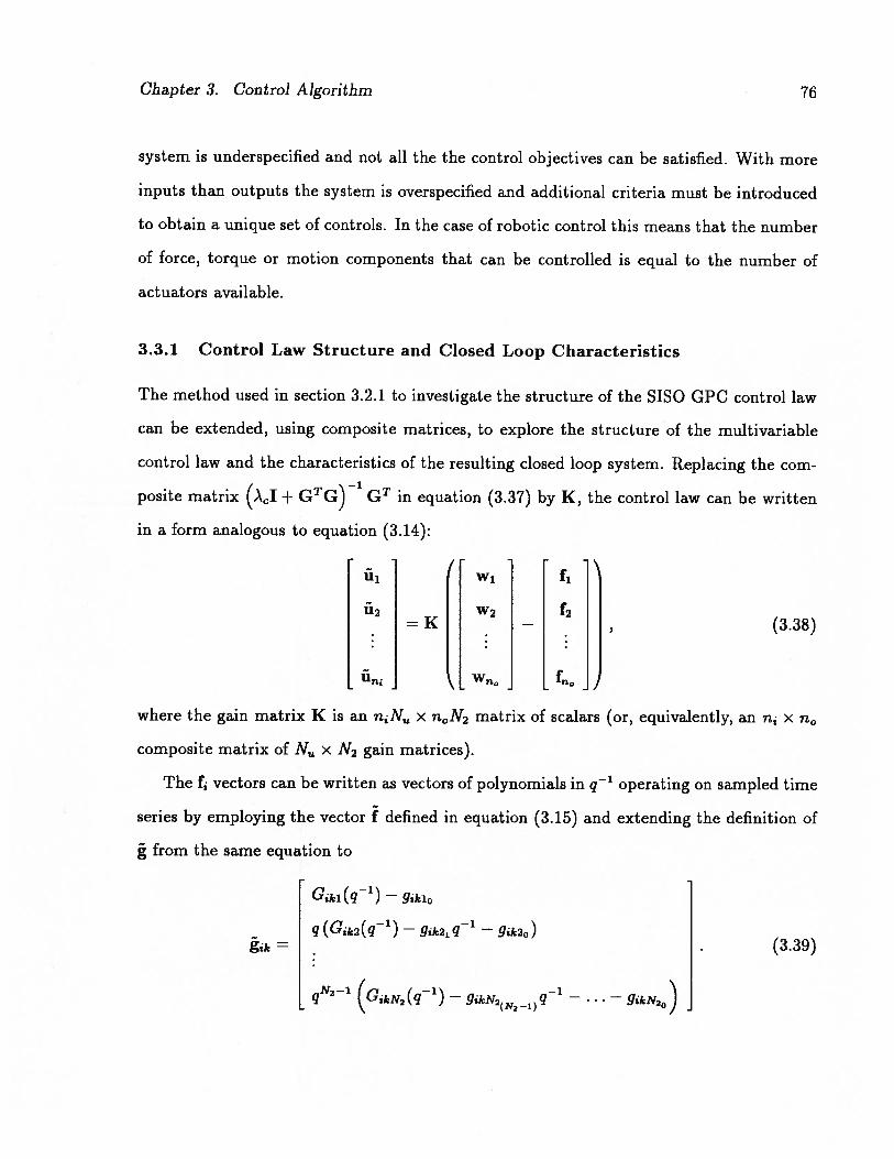
Chapter 3. Control Algorithm 76
system is underspecified and not all the the control objectives can be satisfied. With more
inputs than outputs the system is overspecified and additional criteria must be introduced
to obtain a unique set of controls. In the case of robotic control this means that the number
of force, torque or motion components that can be controlled is equal to the number of
actuators available.
3.3.1 Control Law Structure and Closed Loop Characteristics
The method used in section 3.2.1 to investigate the structure of the SISO GPO control law
can be extended, using composite matrices, to explore the structure of the multivariable
control law and the characteristics of the resulting closed ioop system. Replacing the com
posite matrix + GTG)1
GT in equation (3.37) by K, the control law can be written
in a form analogous to equation (3.14):
ü1 w1
=K: — :
(3.38)
w,
where the gain matrix K is an nN x m0N2 matrix of scalars (or, equivalently, an n x n0
composite matrix of N x N2 gain matrices).
The f vectors can be written as vectors of polynomials in q operating on sampled time
series by employing the vector f defined in equation (3.15) and extending the definition of
from the same equation to
I_v I, —1\‘-ii.q i Yzklo
—1 —1q (Gk2(q ) gk21q — gik2o)= (3.39)
qN2l (GjkN2(q_1)— — . . .
— gikN2o)

Chapter 3. Control Algorithm 77
Thus
1 0 0 yi(t) Au1(t)
= 0 0 y(t) + Lu(t). (3.40)
fN2 0 0 yn(t) n1 g2 Lu(t)
Likewise, employing the vectors q and q, defined in equation (3.16), the vectors of iiks
and ws are written in the form of polynomials in q’ operating on sampled time series:
ii q 0 0 zui(t)
112 = 0 q, •.• 0 Au2(t)(3.41)
0 0 q.
and
q 0 0 wi(t)
W2 = 0 q 0 W2(t)(3.42)
w,, 0 0 q
Using these expressions the control law can be rewritten as
ui(t) wi(t) yi(t)
U2(t) W2(t) y2(t)(quI+KG)z =KqI KfI . (343)
u(t) w0(t)
This is a set of n1N difference equations.

Chapter 3. Control Algorithm 78
With the difference equations (3.24) which describe the open loop dynamics of the system
expressed in matrix operator form:
yi(t) u(t)
A(q’)y2(t)
= B(q’)q1u2(t)
(344)
y(t) u(t)
where
B11(q1) B12(q’) . . . B1(q’)
B21(q1) B22(q1) ... B2(q)
Bi(q1)B02(q1) ... B0(q’)
the vector of y2(t)s can be eliminated to yield
ui(t) wi(t)
w2(t)(qui + KG) AA + KfIBq’]
:= AKqI
:(3.45)
u(t) w0(t)
This expression is a closed ioop transfer function relationship between the setpoints and the
control inputs. Manipulation of equations (3.43) and (3.44) to arrive at the more conven
tional closed ioop transfer function representation relating the setpoints to the outputs is
problematic because it involves the inversion of the B matrix of q’ polynomial operators.
Fortunately, because the inputs and outputs are linearly related by the control law, this
difficulty affects only the eigenvectors of the closed ioop representation; the eigenvalues of
the matrix on the left hand side of equation (3.45) are the poles of the closed ioop system.
The calculation of the approximate, continuous time domain, closed ioop characteristics
from these poles is shown in Chapter 5 to be a useful method of tuning the multivariable
control law.

Chapter 3. Control Algorithm 79
3.4 Static Equilibrium Bias Term
Generic, linear input/output models are used to describe the systems on which the deriva
tions of the SISO GPC algorithm (section 3.2) and its multivariable counterpart (section 3.3)
are based. While this structure results in a control algorithm that is applicable to many
diverse systems, it is desirable to customise the control algorithm for a particular system
by using additional knowledge about that system and thereby improve the control. In the
case of control of contact forces between a robotic manipulator and its environment the
dynamic model of the system can be used to form a relationship between the desired force
levels (setpoints) and the actuator input levels required to maintain those forces when the
system is in static equilibrium. This information is introduced into the control algorithm by
augmenting the cost function with a term that weights the sum of squares of the deviation
of the actual total control input levels from the calculated static equilibrium levels. This
term is referred to as a static equilibrium bias term and its addition to both the SISO and
multivariable predictive control algorithms is an original contribution of this thesis.
The static equilibrium bias term acts as a proportional feedforward term in the control
law. This term has the beneficial effect of reducing the step response rise time but this
improvement comes at the expense of introducing a small amount of overshoot. Simulation
results discussed in section 5.3.4 illustrate these characteristics.
The function which maps the set of setpoint levels, {w, i = 1,. . . , n0}, at a given time
step onto the corresponding set of static equilibrium control inputs, {Ük, k = 1,. . . ,n}, is
obtained from the equations of motion of the system and the contact force model. Details
of the necessary manipulations of equations (2.47) through (2.52), (2.56) and (2.57) to
obtain the mapping function for the case of a two flexible link manipulator are shown in
Appendix C.

Chapter 3. Control Algorithm 80
Defining vectors, analogous to the vector of future setpoints (equation (3.30)), for the
actual control inputs, Uk, and the calculated static equilibrium inputs, Uk,
= { u(t+ 1) uk( + 2) Uk(t + Nu)] k = 1,... ,n (3.46)
and
= [Ük( + 1) Uk(t + 2) tLk(t + N) k 1,. . . ,n, (3.47)
the static equilibrium bias term for the cost function is the sum of squares of differences
between Uk and
- T -
Jse >Z(uk_tlk) (Uk —Uk). (3.48)
This term is weighted by a factor, ,X, and added to the predicted output error and incre
mental control energy cost function terms given by equations (3.32) to yield the overall cost
function
J2 + .X8eJse
=+ cÜÜk + \se(Uk — uk)T (Uk Uk). (3.49)
The vector of control inputs, Uk, is formed from the (previously defined) vector of control
input increments, Uk, by adding the future increments to the current input value, u= Uk(t).
Defining i as a unit vector and L as a unit lower triangular matrix,
1 100...0
1 110...0IL= . and L=
1 1l1...1
Uk can be written as:
Uk = u + LUk. (3.50)

Chapter 3. Control Algorithm 81
Substituting equation (3.50) into equation (3.49) yields:
J3 = : eej + \c Ü U + se (u H- Lfik Uk) + Lük — Uk). (3.51)
Since J3 is a linear combination of J2 and Jse the principle of superposition allows the results
of the expansion and minimisation of 18e to be added to the results given by equation (3.35)
to obtain the overall control law. Expanding Jse and differentiating with respect to Urn (an
arbitrary member of the set of control input increment vectors, see section B.2 for details)
gives:
(3.52)
The set of control input increments, {Um,m = 1,... ,n}, that minimises Jse is given by:
OJse--—=0, m=1,...,m. (3.53)oum
Applied to equation (3.52), this condition yields:
LTLIIm LT (m —uji.), rn= 1,...,n2. (3.54)
Adding this set of equations, weighted by .se, to (3.35) gives
>GnGikUk +AcUm+seLTLUm = >G (w _fj)+AeLT (Urn _UjL),irzl kr1 jzl
m=1,...,n (3.55)
an augmented system of linear algebraic equations which can be solved for {Um,m =
1,.. . ,n2}. These equations can be written in matrix form similar to equation (3.36):
G G’1 ... G11 G12 ... G11
G G ... G2 G21 G22 ... G2
... G02

Chapter 3. Control Algorithm 82
LTL 0
0 LTL+.\3e
0
0
L
U1 -
U2
Un1 -
— fi
— f2
— fTl0
— 0U1 — U1,i
— 0U2 — U2L
Wi
W2
wna
0 0 ... L’
‘T rITLW11 ‘21
GT iT CIT12 ‘22 n02
-‘iT CIT T“1n1 ‘2n non
)iseLT 0 ... 0
0 AseLT... 0
0 0 ... .X3eLT
+ (3.56)
iin—
u1p
This linear system has the same dimensions as equation (3.36). The matrix LT is N x
N and the vector of static equilibrium biases on the right hand side is n2N x 1. The
requirement of an equal number of inputs and outputs for a unique solution also holds.
With the matrix of Gk terms represented by a composite matrix; G, equation (3.56)
can be rewritten as
w1—f1
w2—f2= K1 (3.57)
w0 — f — u,i -

Chapter 3. Control Algorithm 83
where—1
LTL 0 ... 0
o LTL... 0K1 = )I + GTG +
: : :GT (3.58)
o o ... LTL
and
—1LTL 0 ... 0 LT 0 ... 0
o LTL... 0 0 LT ... o
K2A3e AcI+GTG+Ase . . . .
o o ... LTL 0 0 ... LT
(3.59)
Comparing this result to equation (3.37) it is evident that the control laws differ slightly in
the structure of the inverted quantity in K and K1. The more significant difference is the
addition of the second (K2) term in equation (3.57). This term make a contribution to the
control input which is proportional to the difference between the expected static equilibrium
inputs (u) and the current levels (u). The magnitude of the contribution is governed by
the value of ?. Thus, the term produces a proportional feedforward action in the control
law.
3.5 Control Algorithm Parameters and Tuning
The multivariable predictive control algorithm has four tuning parameters:
1. N2, the prediction horizon;
2. N, the control horizon;
3. ), the input increment weighting factor; and,

Chapter 3. Control Algorithm 84
‘ae, the static equilibrium bias term weighting factor.
The prediction horizon specifies the number of time steps into the future for which
predicted system outputs will be calculated and included in the control law. Clarke, et
al. [29] recommend that N2 be set comparable to the rise time of the open ioop system.
The prediction horizon should also be far enough in the future to include the negative-going
part of a nonminimum phase open ioop response. Too short a prediction horizon causes
the controller to work with insufficient information and the control is likely to be poor or
even unstable. Increasing N2 causes the poles of the closed ioop system to move toward the
locations of the open loop poles.
The control horizon is the number of time steps in the future after which the control
input level will be held constant, that is, all future increments set to zero. This horizon
has significant effect on the computational load of the algorithm since the left hand side
matrix of equation (3.56) (which must be inverted) has dimensions n0N x n2N. Clarke,
et al. [29] recommend that N,. be greater than or equal to the number of unstable or poorly
damped zeros in the open ioop system. In the multivariable form of the algorithm the
control horizon should be at least equal to the number of inputs to the system. Increasing
N,. generally increases the magnitude and rate of change of the control input signals. To
a certain extent this increased activity leads to higher performance control but too large
a value for N,. may result in excessive ringing of the control signals and significant high
frequency components in the step response transients.
The input increment weighting factor governs the contribution to the cost function of
the sum of squares of control input increments term, that is, the incremental control energy.
With ) set to zero this term has no effect on the cost function or the control law. The
use of a nonzero has been found to introduce a pole on the negative real axis into the
continuous time representation of the closed loop system. This pole moves toward the origin

Chapter 3. Control Algorithm 85
as is increased. In the context of contact force control this additional pole may have a
stabilising effect for the case of a rigid link manipulator but its interaction with the poles
due to other modes in the flexible link case generally results in a slower step response.
The static equilibrium bias term weighting factor controls the extent to which that term
influences the control law. A value of zero for Xse results in no static equilibrium bias.
Increasing Ase causes the control inputs to tend toward the calculated static equilibrium
values. Thus the static equilibrium bias term can be viewed as a proportional feedforward
term in the control law with a gain related to )se. The fact that the contribution of this
term to the overall control input signal is larger when the output is far from the setpoint
than when it is near means that the response will generally be faster as ) is increased.
However, as the results in Chapter 5 show, this performance improvement comes at the
expense of introducing overshoot into the response.
Clarke, et al. [29] include one additional parameter in the GPC algorithm: the delay
horizon, N1. This horizon serves to reduce the computational load of the algorithm in
situations where there is a delay between the application of a control input increment and
its effect appearing on system outputs. Such situations are common in process control
applications but in the case of robotic force control there is no delay, provided that the
control law calculations can be completed with a single time step, and N1 is set to 1.
In principle, a different prediction horizon value, N22, could be used for each output in
the multivariable algorithm. Similarly, independent values for N, X, and Ase for each input
could also be specified. The resulting algorithm is substantially more complex to implement
and no clear advantage can be seen in using multiple horizon and weighting factor values.

Chapter 3. Control Algorithm 86
3.6 Parameter Estimation
As was noted at the beginning of this chapter the inherently stiff nature of the dynamics of
a manipulator in contact with its environment as well as the strong coupling and nonlinear
dynamic effects present a significant challenge in the design of a controller for contact
forces. This challenge is met, in part, by implementing the control algorithm in an explicitly
adaptive context, that is, the values of the coefficients of the polynomials in the controller
model (equation (3.24)) are estimated on-line from the time series of calculated control
inputs and sensed contact force outputs. This parameter estimation is accomplished by a
recursive least squares (RLS) algorithm.
The basic RLS algorithm [77] is described by a pair of update equations, one for the
vector of parameter estimates,9 and the other for the covariance matrix, P:
+ 1 k(Yk — ‘k-i) (3.60)
1) —
rki ((‘k ‘I’kIE k — ‘ k—i
— 1 .iT 0 > U,
I + Yj E k—i ‘Pk
where cbk is the regressor vector of input and output data values and yk is the value of
the system output at time step k. This algorithm has optimal convergence and stability
properties when the parameters to be estimated are time invariant. Unfortunately, the basic
algorithm is unsuitable for tracking time varying parameters because its gain converges to
zero. A large number of modified RLS algorithm have been developed to overcome this and
other limitations.
In the early stages of the research the U/D RLS algorithm of Bierman [83] was employed.
The U/D RLS algorithm factorises the covariance matrix into the product of an upper tri
angular and a diagonal matrix (U/D factorisation) and thereby ensures that the covariance
matrix will always be positive definite. Tracking of time varying parameters is facilitated
by use of an exponential forgetting factor to weight older data less heavily than new. The

Chapter 3. Control Algorithm 87
effect of this weighting is to establish a nonzero lower bound on the minimum eigenvalue
of the covariance matrix and thereby prevent the occurrence of zero elements in the gain
term of the parameter update equation (3.60). Unfortunately, exponential forgetting can,
in the absence of sufficient excitation in the input data, lead to covariance wind-up; the
unbounded growth of the eigenvalues of the covariance matrix which leads to corresponding
growth of the elements in the gain term of equation (3.60).
All of the adaptive control results presented in Chapter 5 employ a newer modified RLS
algorithm developed, by Salgado, et al. [841, known as EFRA which stands for Exponential
Forgetting and Resetting Algorithm. As well as using the exponential data weighting nec
essary to track time varying parameters the EFRA algorithm also incorporates exponential
resetting of the covariance matrix in such a way as to give new data unprejudiced treatment.
Furthermore, the algorithm provides a means of establishing bounds on the maximum and
minimum eigenvalues of the covariance matrix, thus avoiding covariance wind-up. The
update equations for EFRA are:
=e +LePklbk
(Yk-
(3.62)
=— ePk_1kPk_1
+e1 SeP_i, (3.63)l+41Pk—1çbk
where ce, /3e, 8e, and ) are constants. Salgado, et al. [84] give the following guidelines for
the values of these constants:
• adjusts the gain of the least squares algorithm; typically e E [0.1, 0.5];
• /3e is a small constant which is directly related to the minimum eigenvalue of P;
typically/3e [0,0.01];
• 6e is a small constant that is inversely related to the maximum eigenvalue of P;
typically Se E [0, 0.011;
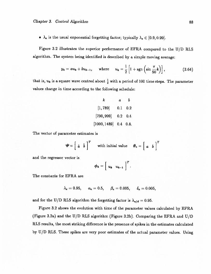
Chapter 3. Control Algorithm 88
Xe is the usual exponential forgetting factor; typically A, E [0.9,0.99].
Figure 3.2 illustrates the superior performance of EFRA compared to the U/D RLS
algorithm. The system being identified is described by a simple moving average:
Yk auk + buk_l, where Uk = [i + sgn (sin k)], (3.64)
that is, Uk is a square wave centred about with a period of 100 time steps. The parameter
values change in time according to the following schedule:
k a b
[1,789] 0.1 0.2
[790,999] 0.2 0.4
[1000, 1489] 0.4 0.8.
The vector of parameter estimates is
=
T
with initial value 90= [ a b
and the regressor vector is
cIJk—_[Uk Uk_lj.
The constants for EFRA are
= 0.95, ae = 0.5, 13e = 0.005, Se = 0.005,
and for the U/D RLS algorithm the forgetting factor is ?u/d 0.95.
Figure 3.2 shows the evolution with time of the parameter values calculated by EFRA
(Figure 3.2a) and the U/D RLS algorithm (Figure 3.2b). Comparing the EFRA and U/D
RLS results, the most striking difference is the presence of spikes in the estimates calculated
by U/D RLS. These spikes are very poor estimates of the actual parameter values. Using

Chapter 3. Control Algorithm
3.5
3.0
2.5
0 2.0ci)i.5E4-.Cl)w .5
0ci)
.5
-2.0
-2.5
-3.00
89
.8
.7
U)C).
00 100 200 300 400 500 600 700 800 900 1000 1100 1200
Time Step
(a) EFRA parameter estimates
100 200 300 400 500 600 700
Time Step800 900 1000 1100 1200
(b) U/D RLS parameter estimates
Figure 3.2: Comparison of EFRA and U/D RLS parameter estimation algorithms.

Chapter 3. Control Algorithm 90
those values in a controller model leads to inaccurate calculation of the required control
inputs which, in turn, yields poor control and perhaps even instability.
Finally, it should be noted that the update equations (3.62) and (3.63) for EFRA are
equally applicable to single input, single output systems as above and to multivariable
systems of the form of equation (3.24). For a multivariable system the vector of parameter
estimates and the regressor vector are augmented to include the coefficients and data from
each of the inputs:
= [ a1 ... anai b10 ... b1b1 ... bno ...
]T
(3.65)
and
ik= { Yk ... Yk—na Ulk ... U1(k_nbi) ... ...
(3.66)
At each time step the estimation algorithm must be executed once for each system output.
3.7 Adaptive Controller Implementation
The overall control strategy implementation is shown in Figure 3.3. This strategy allows
control of both the contact forces and the gross motions of the manipulator when it is not
in contact. In the latter case the joint angles or velocities are taken as the system outputs.
Due to the discontinuous nature of the system dynamics, the transfer function models used
in these two modes of control are necessarily distinct and of different order. The force and
motion models are identified and maintained in parallel so that switching between control
modes can be accomplished smoothly. The contact control logic block controls selection
of the appropriate (force or motion) control law, based on data from the force sensor and
joint encoders and the trajectory planner, as well as controlling whether or not the transfer
function models are updated by the parameter estimation blocks. The force and motion

Chapter 3. Control Algorithm 91
Figure 3.3: Control strategy block diagram.

Chapter 3. Control Algorithm 92
setpoint programs are assumed to be provided by the higher levels of the control hierarchy
which include the operator, a task planner and a trajectory generator.
With the parameter estimation blocks enabled, the controller is explicitly adaptive. At
each time step the coefficients of the transfer function model currently in use are estimated
using the Exponential Forgetting and Resetting Algorithm (EFRA) [84]. The estimated
coefficients are assumed to be instantaneously exact and the set of control input increments
for that time step is calculated. At the next time step a new set of coefficients is estimated
and used to calculate a new set of control input increments.
The performance of the overall control strategy in situations which necessitate switching
between force and motion control is discussed in section 5.4.
3.8 Stability and Convergence
Stability and convergence are important and difficult issues in the design of adaptive con
trollers. For a given set of values for the model coefficients the stability of the control
algorithm part of an adaptive controller can be considered. In the case of the CPC al
gorithm it has been shown [33] that, with a finite prediction horizon (N2), the resulting
closed—loop control is stable provided that:
1. the open—loop system model is stabilizable and detectable,
2. the delay (N1) and control (Nu) horizon are selected with respect to the number of
system model states (n) such that N = N1 n and N2 — N1 n — 1, and
3. the control weighting factor () is small (i.e. = —* 0).
It should be noted that this is only a sufficient (but not necessary) condition for which
stability of the algorithm can be proven. The GPC algorithm is demonstrably stable for
sets of parameters (N1,N2,Nu, and ?) other than those which satisfy the above conditions.

Chapter 3. Control Algorithm 93
Given this result, the issue of stability of the adaptive GPO controller becomes one
of whether or not the system identification algorithm provides model coefficients which
describe a stabilizable and detectable open—loop system. The Exponential Forgetting and
Resetting system identification algorithm (EFRA) [84] discussed in section 3.6 is of the
recursive least squares (RLS) family. The asymptotic properties of this type of algorithm
are well established [85]. However, those asymptotic properties are concerned with the “best
possible predictor” for the system which the algorithm can determine. The relationship
between that predictor and the stabilizable and detectable model of the open—loop system
which is required for stability of the adaptive GPO controller is dependent on such factors
as the number of model coefficients and the system input.
In light of these factors, it is evident that an analysis of the dynamics of the system
to be controlled is necessary to select an appropriate number of model coefficients and to
select initial values for those coefficients which satisfy the stabilizability and detectability
requirements of the adaptive GPO algorithm. Augmentation of that analysis with a series
of identification experiments on the system would most certainly be beneficial.
39 Summary
This chapter presents the development of a manipulator contact force control strategy based
on an explicitly adaptive implementation of a predictive control algorithm. The control
algorithm is based on the Generalised Predictive Control (GPO) algorithm of Clarke, et
at. [29]. This form of predictive control algorithm was selected over other control methods
because it incorporates the following desirable features:
• inherent integral action;
• setpoint tracking;

Chapter 3. Control Algorithm 94
• ease of implementation in explicitly adaptive, digital form, and;
• inclusion of non-minimum phase and lightly damped mode characteristics in predictor
model.
The primary contributions of this chapter are the extension of the generic predictive control
algorithm with a new static equilibrium bias term that allows knowledge of the system
dynamics to be employed to improve the controller performance, development of a new
formulation of the closed loop characteristic polynomial which is directly useful in controller
tuning, and introduction of a contact control logic level in the control hierarchy to deal with
the discontinuity involved in making and breaking contact between the manipulator tip and
the environment surface.

Chapter 4
Dynamics and Control Simulation — TWOFLEX
4.1 Introduction
The simulation computer program TWOFLEX incorporates the dynamic model of the pla
nar two flexible link manipulator and deformable environment derived in Chapter 2 and
the adaptive single- and multi-variable long range predictive control algorithms derived in
Chapter 3. The code is written in FORTRAN. It was originally developed on a VaxStation
3200 under the VMS operating system and subsequently ported to a Sun SparcStation
under SunOS. Both versions of the program use double precision arithmetic throughout.
Results of the runs are stored in text files as tabulated time series of related groups of vari
ables and as plots of the evolution of selected variables with time. The dynamics models
of the links, actuator, and contact regions are coded in such a way that the program can
easily simulate subsystems of the two flexible link manipulator system (e.g. a single rigid
or flexible link or two rigid links). Likewise, the controller structure to be simulated (i.e.
SISO or multivariable, adaptive or constant parameter, force, motion or combined control,
etc.) is also selectable. The particular configuration of dynamics model and controller to
be used for a given run is specified by a set of parameter values which are read from a data
file each time TWOFLEX commences execution.
This chapter begins with a description of the overall structure of the TWOFLEX program in
section 4.2. Section 4.3 presents the details of the numerical integration of the equations of
motion for the manipulator/environment system. The description of the program concludes
95

Chapter 4. Dynamics and Control Simulation — TWOFLEX 96
in section 4.4 with a discussion of the routines that simulate the discrete time control algo
rithm. The structure of these various parts of the program are illustrated with flowcharts.
A complete listing of the documented source code for the TWOFLEX program and the associ
ated subroutine libraries (approximately 18,200 lines of FORTRAN code in total) is available
in the UBC CAMROL (Computer Aided Manufacturing and Robotics Laboratory) Report
number R.92—2 [34]. Section 4.5 describes several tests which were conducted to validate
the operation of the program by comparison to a simulation of a multibody space station
based flexible manipulator developed by Mah [35]. The chapter concludes with a summary
of the features of the TWOFLEX code.
4.2 General Description of the TWOFLEX Program
A flowchart of the overall structure of the TWOFLEX program is shown in Figure 4.1. The
steps in the code execution, as represented in Figure 4.1, are described in the following
paragraphs.
The program begins with the reading and processing of data from the input files. These
data specify the configuration of the system for the run, the initial conditions, and, nu
merous logical flags to select various options in the code. The main input file for a typical
run consists of about 50 lines of data. The input routines use free formatting and permit
comments to be interspersed with the data by placing them on lines beginning with an *
character. Auxiliary input files contain the setpoint information for the controller. Process
ing of the input data includes calculation of various quantities needed in the simulation.
In particular, values of the mode shape functions and the corresponding inertia integral
factors, ‘mkt, for the equations of motion are calculated at this point.
Output initialisation involves opening of, and writing headings to, the various files which
will receive output data as the simulation proceeds. A summary of the configuration for

Chapter 4. Dynamics and Control Simulation — TWOFLEX 97
Figure 4.1: Flowchart of the overall structure of the TWOFLEX dynamics and control simulation program.
False

Chapter 4. Dynamics and Control Simulation — TWOFLEX 98
the run is written out at this point, both to serve as a reference when reviewing stored run
results and to provide a check on the validity of the input data.
Next, the initial state of contact is checked. If the initial conditions are such that the
apparent separation between the tip of the manipulator and the surface of the environment
is negative, contact exists and the components of the contact force are calculated. In the
case of positive separation, contact does not exist and the contact force is zero.
Following these initialisation steps, the main loop of the simulation begins. This loop
is controlled by the value of the integration time variable, t2, and proceeds in steps of dt.
The value of dt, is generally selected to be quite small since the main loop includes the
integration of the equations of motion which simulates the response of a continuous time
system. Within the main ioop, the integration time, is checked to determine if it is modulo
dtd, the discrete time step. Only if that condition is true are the discrete time control
algorithm routines executed.
The discrete time control algorithm consists of the contact control logic, the parameter
estimation algorithm and the control algorithm itself, which calculates the input signals to
be applied to the actuators. Section 4.4 describes these parts of the program in detail.
Flags in the input data file can be set to disable the execution of the control algorithm
and instead apply one of a set of open loop input signals to the system. The available open
loop input signals include impulse, step, ramp, square wave, sine wave and white noise.
These signals are useful in observing the forced, but uncontrolled, response of the system.
Regardless of the source of the input signal, the main loop continues with the integra
tion of the equations of motion over the time interval dt. The DGEAR routine from the
International Mathematical and Statistical Library (IMSL) [86] is used for the integration.
A discussion of the features of DGEAR and the details of the form of the equations which are
actually integrated is included in section 4.3.

Chapter 4. Dynamics and Control Simulation — TWOFLEX 99
After completion of the integration time step, the new state of the system is checked to
determine if the contact state has changed. If the manipulator tip is in contact with the
environment surface the components of the contact force are calculated. The new state of
the system and a collection of data calculated from it are written as text to the time series
output data files. Some of those values are also stored for later plotting.
Finally, the system state is checked to determine if any of a set of limits on quantities
such as the manipulator joint angles have been surpassed. This limit checking allows runs in
which the system state “blows up” to be halted before the entire duration of the integration
has been calculated while preserving, for later analysis, the evolution of the response up to
the time at which the run is terminated.
If the time specified for the end of the integration has not been reached the main loop
is repeated, after incrementing the integration time, t, by dt2. When the loop has been
completed for the last time the final results of the simulation are written to the output data
files and plotted.
4.3 Integration of Equations of Motion
The equations of motion for the manipulator/environment system are integrated numerically
using the IMSL routine DGEAR to yield the approximate continuous time response of the
system. The DGEAPL routine is based on the work of Gear [87]. It is a backward differencing
method, meaning that it uses backward difference formulae to approximate derivatives.
The algorithm incorporates adaptive step size selection which allows optimal performance
to be achieved by subdividing the interval over which the integration is being performed as
necessitated by the characteristics of the equations, without user intervention. The DGEAR
routine was selected for two reasons:
1. it is specifically designed for integration of stiff systems of differential equations, and,

Chapter 4. Dynamics and Control Simulation — TWOFLEX 100
2. it is well suited for integrations from which results are required at frequent, small
increments of the independent variable.
A system of differential equations is said to be stiff if there are two or more very different
scales of the independent variable which simultaneously effect the dependent variables [88].
A more mathematically rigorous definition [86] is that the system of first order ordinary
differential equations given as
y’=f(x,y1,y2,...,y) (4.1)
ofis stiff if some of the eigenvalues of the Jacobian matrix of partial deLivatives, are
large and negative. As was noted in Chapter 3, the system of differential equations (2.47)
through (2.52) is stiff because the natural frequencies of the system can easily span several
orders of magnitude and thus the generalised coordinates are composed of variations with
several, widely varying time scales.
The simulation uses a small time step, dt1, in the main integration ioop in order to
adequately reflect the continuous time nature of the dynamics in contrast to the discrete time
control algorithm. Small time steps are also required to adequately resolve high frequency
components of the response in graphical presentation of the simulation results. Finally,
and most importantly, small integration time steps are necessary to properly detect the
making and breaking of contact between the manipulator tip and the environment. If too
large a time step is used the manipulator will appear to penetrate the environment during
the time step in which contact is made and an erroneously large transient contact force will
result. The maximum permissible time step is dependent on the stiffnesses of the contacting
surfaces.

Chapter 4. Dynamics and Control Simulation — TWOFLEX 101
The DGEAR routine integrates systems of first order, ordinary differential equations.
Equations (2.47) through (2.52) are a system of second order ordinary differential equa
tions of the form:
Jj=b(q,4). (4.2)
Such a system is easily transformed to first order by the substitution:
q1 = q and q2 = 4 (4.3)
which yields,
I 0 41 q2. (4.4)
0 J q b(q1,q2)
In this representation, J is the generalised inertia matrix, q1 is the vector of generalised
coordinates, 4i = q is the vector of generalised velocities, 42 is the vector of generalised
accelerations and b (q1,q2) is the vector of values of the right hand sides of the equations
of motion. The matrices, I and 0, are identity and zero matrices, respectively. The state
vector for the system is [q1q2]T•
The DGEAR routine calls a user provided routine which must return the first time deriva
tive of the state vector. The generalised velocity part of that vector is simply copied from
the most recently calculated system state and the generalised acceleration part is calculated
by the steps shown in the flowchart in Figure 4.2. Since the dynamics of the DC motor
actuators are represented by first order, ordinary differential equations the state variables
from those models are simply concatenated onto the end of the state vector. Likewise, right
hand sides of the actuator model equations are concatenated onto the right hand side of
equations (4.4) for simultaneous solution with the equations of motion.

Chapter 4. Dynamics and Control Simulation — TWOFLEX 102
Calculate InertiaMatrix
1Calculate Right Hand
L Side Vector
1Add actuator couplingterms to inertia matrix
and RHS vector
‘I;Invert Inertia
Matrix
Multiply RHS vectorby Inertia Matrix Inverse
to yield GeneralisedAcceleration Vector
Figure 4.2: Flowchart of the calculation of the generalised acceleration vector.
4.4 Discrete Time Control Algorithm
The control algorithm described in Chapter 3 is implemented in a series of subroutines which
are executed only when the integration ioop time, t, is a whole multiple of the discrete time
step, dtd, (that is, t mod dtd = 0). Figure 4.3 shows a flowchart of the steps in the control
algorithm.
The first step in the control algorithm is the contact control logic block. This part of the
algorithm takes, as inputs, signals from the manipulator force sensor and joint encoders,
information from the trajectory planner and instructions from the operator. These data
are analysed and used to generate the sequences of future setpoints, to determine which
control mode (force or motion) should be used, and to decide whether or not the parameter
estimation algorithm should be activated to update the controller model coefficients. The
primary purpose of the contact control logic is to govern the actions of the control algorithm

Chapter 4. Dynamics and Control Simulation TWOFLEX 103
hitialise DiophantineIdentity Polynomials
for Recursion Formulae
Figure 4.3: Flowchart of the discrete time control algorithm.

Chapter 4. Dynamics and Control Simulation — TWOFLEX 104
during the time period immediately before and after a change in the contact state. This
function is particularly important when the manipulator unexpectedly comes into contact
with the environment, in which case the impact velocity may be large and result in contact
force transients which the predictive control algorithm cannot immediately compensate for.
Some examples of the categories of programs that the contact control logic can execute are:
• assuming the trajectory planner has an accurate world model of the manipulator and
its surroundings, the speed of approach to a surface and the time at which the control
should be switched between motion to force modes can be specified and the contact
control logic generates appropriate setpoint sequences and switching signals;
• in unknown or uncertain surroundings the contact control logic switches the control
mode from motion to force when a nonzero force signal is sensed and from force to
motion when the signal goes to zero;
• when contact is sensed by the force sensor the contact control logic switches to force
control mode and briefly modifies the contact force setpoint sequence from that pro
vided by the trajectory planner to a form suitable to compensate for the contact force
transient; the setpoint modification is based on an heuristic rule.
Contact control logic programs are discussed in more detail, with examples of the resulting
closed ioop responses in Chapter 5.
If the contact control logic program specifies that the control should be adaptive in
the current time step the coefficients of the controller model are updated using one of the
parameter estimation algorithms discussed in section 3.6. Both the U/D RLS algorithm
and EFRA are implemented in the TWOFLEX code. The algorithm to be used is selected by
a flag set in the input data file. The algorithm parameters are also included in the data
read at the beginning of the run.
Chapter 4. Dynamics and Control Simulation — TWOFLEX 105
The actual calculation of the control input signal increments begins with the initialisation
of the polynomial coefficients in the Diophantine identity recursion formulae. With those
coefficients and the coefficients from the controller model, the free response vectors, f1, for
one time step into the future are calculated.
Following the initialisation step, the Diophantine identity polynomial coefficients and
free response vectors are calculated for each of the future time steps up to the prediction
horizon, N2.
The final step in the predictive part of the algorithm is the calculation of the future
static equilibrium input sequences from the specified future setpoint sequences. This step
is only applicable in the case of force control since a direct relationship is available between
desired contact forces and the static equilibrium input levels that would be required to
produce them.
For computational efficiency the control horizon is checked before beginning to calculate
the control input increments. If N = 1 the calculation can be quickly performed as a scalar
operation in the case of a SISO system or by Cramer’s rule for a two input, two output
MIMO system. For N > 1, the future step response matrices, G1k, and their transposes
are formed and the left hand side matrix and right hand side vector terms in equation (3.56)
are constructed. The system of linear algebraic equations described by these terms is solved
for the sequences of future control input increments. Finally, the control input increments
for the next time step are added to the control input signals.
The entire discrete time control algorithm described above is embedded in a general
input calculation subroutine in the TWOFLEX code. That routine uses flags set in the input
data file to select the type of input to be used, either the control algorithm or the one of
the open loop inputs described in section 4.2. The input calculation routine also applies
the appropriate actuator saturation limits to the inputs.

Chapter 4. Dynamics and Control Simulation — TWOFLEX 106
4.5 Validation
The simulation of the unforced manipulator dynamics was validated by comparison with the
results of a program developed by Mah [35]. Mah’s program simulates the dynamics of an
orbiting platform and manipulator system modelled as a chain of flexible links connected by
flexible joints. It has been validated [89] against two other simulation programs for related
systems independently developed by Chan [68] and Ng [72]. Two types of validation test
were carried out:
1. the calculated inertia matrices and right hand side vectors for the equations of motion
with specified initial conditions were compared; and,
2. the evolution with time of the values of the generalised coordinates were compared
for simulations of the free response of the system from various initial states.
The calculated initial values of the elements of the inertia matrices and right hand side
vectors were compared for the seven cases listed in Table 4.1. The links were modelled as
1.Om long, 2.0cm diameter aluminium rods in all cases. For each of these cases the initial
inertia matrix and right hand side vector were in agreement to at least three significant
digits. The agreement was least good for terms which depend on the integrals of the
flexible link mode shape functions. This is due to the fact that Mah calculates those
integrals numerically whereas the analytical expression for those integrals for a cantilever
beam are included in the TWOFLEX code.
Comparisons of free response simulation results were made for the three cases listed in
Table 4.2. In the first two cases the links were modeled as 1.Om long, 2.0cm diameter,
aluminium rods. In case 3 the second link was 1.4m long. There is no damping in the
system. Good agreement was obtained in all three cases. Figures 4.4 shows the response of
the joint angle generalised coordinates, 1 and 02, for the first 0.5s of case 2. The results

Chapter 4. Dynamics and Control Simulation — TWOFLEX 107
Initial ConditionsManipulator Structure 8- 62 62 /11 2/’21 ,1’21
Case Link 1 Link 2 [0] [0] [rad/sj [rad/s] [—j [—] [1/sj [1/s]1 Flexible — 0 — 0 0 — 0 —
(1 mode)2 Flexible — 0 0 — LO 0.1 —
(1 mode)3 Rigid Rigid 30 30 0.1 0.1 — — —4 Flexible Flexible 0 0 0 0 0 0 0 0
(1 mode) (1 mode)5 Flexible Rigid 0 0 0 0 0 0 0 0
(1 mode)6 Rigid Flexible 0 0 0 0 0 0 0 0
(1 mode)7 Flexible Flexible 0 0 0 0 1.0 1.0 0.1 0.1
(1 mode) (1 mode)
Table 4.1: Configurations and initial conditions for validation of inertia matrix and righthand side vector terms.
Initial ConditionsManipulator Structure 6 62 2 /‘11 21
- ‘/ii /‘21Case Link 1 Link 2 [0] [] [rad/s] [rad/s] [—] [—] [1/s] [1/s]
1 Rigid Flexible 20 -25 0 0 — 0 — 0.1(1 mode)
2 Flexible Flexible -20 -75 0 0 0.05 -0.1 0 0(1 mode) (1 mode)
3 Flexible Flexible 35 35 0 0 -0.05 0.1 0 0(1 mode) (1 mode)
Table 4.2: Configurations and initial conditions for free response simulation validation runs.

Chapter 4. Dynamics and Control Simulation — TWOFLEX
-70
-75
-80
-85
-90
-95
-100
-105
-110
Time [s]
108
0 .05 .10 .15 .20 .25 .30 .35 .40 .45 .50
Time [s]
(a) 81 response
-4
-6
-8
-10
-12
U)2. -14
-16
-18
-20
-22
U)U)a)L.
a)V
c’J
.50
(b) 82 response
Figure 4.4: Comparison of joint angle responses between TWOFLEX and Mah [89] for freeresponse validation.
0 .05 .10 .15 .20 .25 .30 .35 .40 .45

Chapter 4. Dynamics and Control Simulation — TWOFLEX 109
from the TWOFLEX program and those from Mah [89] are initially coincident and differ by
only a small amounts after 0.5s (5000 integration time steps). The responses of the modal
amplifier generalised coordinates, and ‘çb21, for case 2 are shown in Figure 4.5 and
illustrate the same excellent agreement.
4.6 Summary
The TWOFLEX program is a versatile simulation of the dynamics and control of a planar,
two flexible link manipulator and a deformable environment. The code is modular, ex
tensively documented and includes optionally compiled code to generate debugging output
from almost every subroutine. The integration of the continuous time equations of motion
and the calculation of the discrete time control algorithm are conceptually and structurally
separated in the code, making it a valuable tool for the investigation of both the open and
closed ioop behaviour of the system.
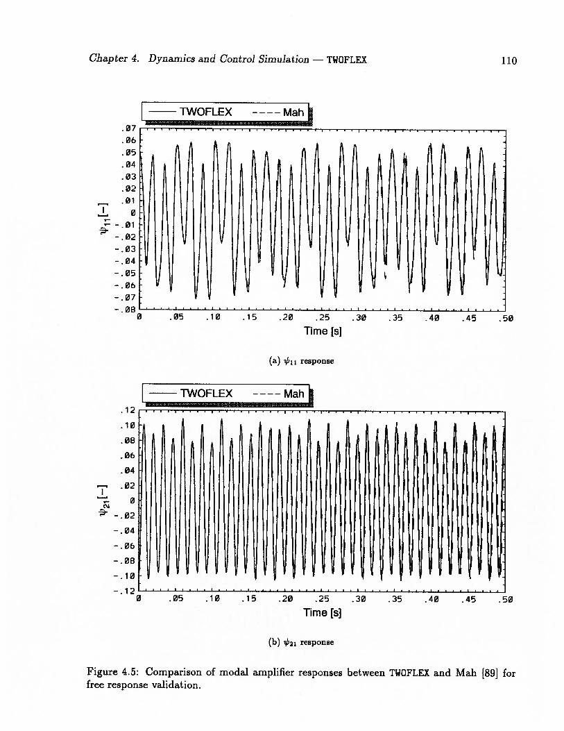
Chapter 4. Dynamics and Control Simulation — TWQFLEX
.07
• 06
• 05
• 04
.03
• 02
.01
0
- .01
- .02-
. 03
- .04-
. 05-
. 06
- .07
- .080
Time [s]
(a) b11 response
110
.12
.10
08
• 06
04
• 02
0
-. 02
—
. 04
-
. 06
-. 08
-.10
-.120
TWOFLEX----j
Time [s]
.05 .10 .15 .20 .25 .30 .35 .40 .45 .50
c’J
.50
(b) 21 response
Figure 4.5: Comparison of modal amplifier responses between TWOFLEX and Mah [89] forfree response validation.
.05 .10 .15 .20 .25 .30 .35 .40 .45

Chapter 5
Force Control Algorithm Performance and Evaluation
5.1 Introduction
This chapter presents results and discussion of the analysis of the dynamics of flexible link
manipulator force control systems and the results of numerous runs of the TWOFLEX dynam
ics and control simulation program. Analysis of the eigenstructure of the system reveals
orderly changes in the dominant natural mode with increasing effective contact stiffness.
These changes have important implications for the selection of the controller parameters.
The simulation results demonstrate the capabilities and evaluate the performance of the
adaptive, multivariable, long range predictive control algorithm developed in Chapter 3.
The results are organised roughly in order of increasing complexity of both the manipula
tor/environment system and the maneuvers which are simulated. This organisation seeks
to emphasise the basic performance of the control algorithm before introducing such com
plications as making and breaking contact, highly nonlinear dynamics, and actuator effects.
An alternative view of the contents of this chapter is shown in Figure 5.1. The topics which
will be addressed can be broadly classified as:
• linear analysis of various manipulator configurations in contact with their working
environments;
• force control step response results for various manipulator configurations; and
• the problem of maintaining control when contact is made or broken.
111

Chapter 5. Force Control Algorithm Performance and Evaluation
I Stop MotionStrategy(5.4.1)
Making andBreaking Contact
Force SetpointModification Strategy
(5.4.2)
112
Figure 5.1: Topics discussed in Chapter 5. Section numbers in which the discussion of eachtopic appears are shown in parenthesis.
Chapter 5. Force Control Algorithm Performance and Evaluation 113
Figure 5.1 indicates the sections in which each of these topics are discussed for each of the
manipulator configurations considered.
The chapter begins with an analysis of the eigenvalues and eigenvectors of the equations
of motion for a single link/environment system. Analytical approximations to the trends
observed in the numerical evaluation of the eigenvalues are developed and the implications
of changes in the modal structure of the system for contact force control are discussed. The
performance of the controller for force control of a single flexible link is discussed in sec
tion 5.3. The calculation, from the physical parameters of a particular link and environment,
of the various parameters and coefficients required by the TWOFLEX program is presented
as well as the derivation of the structure and initial coefficient values of the discrete time
transfer function model for the control algorithm. Simulated step and ramp response results
are shown to demonstrate the performance of the controller. The effects of the controller
horizons and weighting factors in shaping the closed ioop response are also discussed in the
course of Section 5.3. The discontinuous nature of the manipulator/environment system
dynamics is considered in section 5.4 with a discussion of the problems involved in main
taining control during the making and breaking of contact. The use of contact control logic
to overcome those problems is discussed along with the presentation of simulation results
for two different contact control logic strategies. The performance of the multivariable form
of the control algorithm is demonstrated by considering force control for a two link manip
ulators in section 5.5; both rigid link and flexible link manipulators are discussed. Results
of simulations of two links of a prototype model of the DC motor driven Space Station
Mobile Servicing System (MSS) manipulator are presented and discussed in sections 5.6.
The chapter concludes with a summary of the force control algorithm performance. Some
of the work presented in sections 5.3 and 5.4 has already been published [22,27].

Chapter 5. Force Control Algorithm Performance and Evaluation 114
Figure 5.2: Single rigid link in contact with a deformable environment.
5.2 Linear Analysis
This section presents a linear analysis of the dynamics of a single link in contact with
a deformable environment. Particular emphasis is placed on the interaction between the
structural stiffness of the manipulator link and the stiffnesses of the contacting regions of the
link tip and the environment. Using analytical and numerical analysis of the eigenvalues and
eigenvectors of systems of linearised equations of motion it is shown that, for a given link,
this interaction results in distinct changes in the modal structure of the link/environment
system as the effective contact stiffness increases. The implications of these modal changes
for contact force control are discussed.
5.2.1 Rigid Link
Consider first a single rigid link which is the limiting case of infinite structural stiffness. The
equations of motion for the system shown in Figure 5.2 are given in section A.6. Simplifying
those equations by neglecting damping, gravitational effects and the small coupling inertia
L1
1k
/;

Chapter 5. Force Control Algorithm Performance and Evaluation 115
terms between the link and contact mass allows them to be linearised about the nominal
state 6 = 0 and written as:
10181 = ui(t) — k3L1(L1e1 — (5.1)
mcfy = —k3 (E — L61) keyEy, (5.2)
where the generalised coordinates {i, e} are now perturbations about the nominal state.
For the sake of generality the joint torque, r1, has been replaced by a general control input,
ui(t).
To study the eigenstructure of the system these equations are transformed by applying
the Laplace transform and rewriting in matrix form:
1J(s) = ui(s), (5.3)
0
where
= 101s2 + k5L1 —k3L1. (5.4)
—kL1 ms2 + (k3 + k)
The characteristic equation of the system is given by setting the determinant of J(s) to
zero:
=I01ms4+ [I01(k3+ key) + mck8yL] 2 + ksykeyL = 0. (5.5)
The natural frequencies of the system (eigenvalues of J(s)) are given by the roots of equa
tion (5.5). We will first investigate the variation of the natural frequencies with contact
stiffness numerically by considering a 1.Om long, 2.0cm diameter aluminium rod treated
as a rigid link. Given the density of aluminium of 2690kg/rn3 such a link has a mass of
0.8451kg and a moment of inertia about the joint axis of
101 = M1(d)2
+ = 0.2817kg m2. (5.6)

Chapter 5. Force Control Algorithm Performance and Evaluation 116
The contact region masses, m3 and me, are taken as 0.19 each. Figure 5.3 shows the
variation of the natural frequencies of the system with effective contact stiffness ranging
from 50N/m to 5MN/m. The effective contact stiffness is defined as
keffksy+key
(5.7)
The data for this plot was generated by numerical calculation of the eigenvalues of J(s)
for various values of k3 and key. The plot clearly indicates that the natural modes of the
system are well separated in frequency and both frequencies increase in proportion to the
square root of the contact stiffness. These observation can be confirmed analytically using
equation (5.5). Substituting (jw) for s,
I0im(jw)4+ [Ioi(ksy + key) + mkL} (jw)2 + ksykeyL = 0, (5.8)
gives a quadratic equation of the form
ax2+bx+c=0, (5.9)
the roots of which are the squares of the natural frequencies of the system. The coefficients
of equation (5.8) are such that b2 >> 4ac and so the quadratic formula can be approximated
using the binomial expansion to yield:
2 iF 12(sw) = — —b+ b .—4ac)
- :
b+b(14ac)]
1 / 1 4ac 1 4ac2=-
— or (5.10)
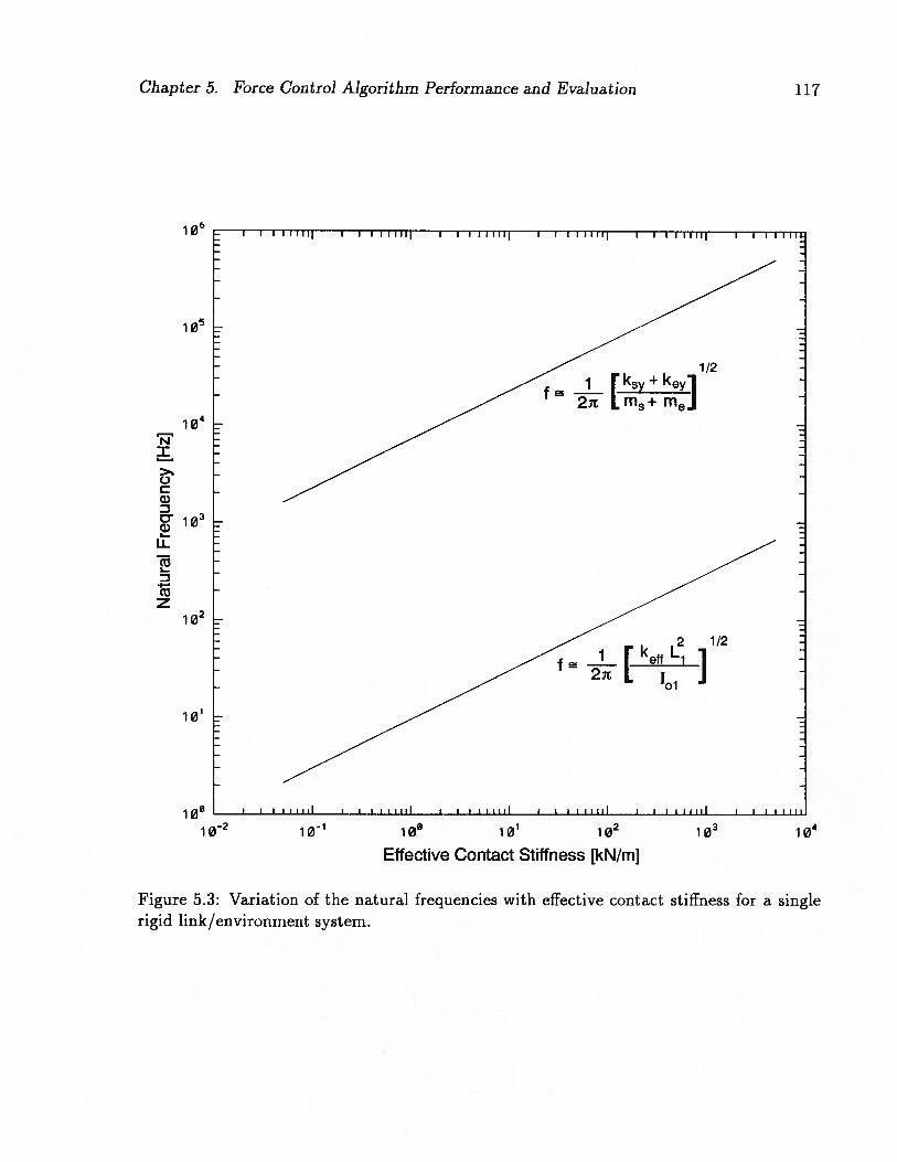
Chapter 5. Force Control Algorithm Performance and Evaluation 117
11111111 I I 1111111 I I 1111111 11111111 I I 1111111 I 111114
iø-
1/2•
1 ksy+key•
2[ms+me -
iø
N
>%C-)C
-a)
:
1/2
ioeI I iii I I liii I i i I i I
10_2 101 i00 101 102 iø i04
Effective Contact Stiffness [kN/m]
Figure &3: Variation of the natural frequencies with effective contact stiffness for a singlerigid link/environment system.
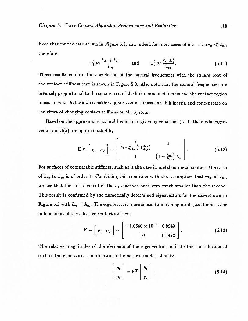
Chapter 5. Force Control Algorithm Performance and Evaluation 118
Note that for the case shown in Figure 5.3, and indeed for most cases of interest, m <<101,
therefore,
2 ksy + keyand
keL(5.11)
m 101
These results confirm the correlation of the natural frequencies with the square root of
the contact stiffness that is shown in Figure 5.3. Also note that the natural frequencies are
inversely proportional to the square root of the link moment of inertia and the contact region
mass. In what follows we consider a given contact mass and link inertia and concentrate on
the effect of changing contact stiffness on the system.
Based on the approximate natural frequencies given by equations (5.11) the modal eigen
vectors of J(s) are approximated by
E [ei e2]1
(5.12)
1 (1_)L
For surfaces of comparable stiffness, such as is the case in metal on metal contact, the ratio
of key to k3 is of order 1. Combining this condition with the assumption that rn,, <<
we see that the first element of the e1 eigenvector is very much smaller than the second.
This result is confirmed by the numerically determined eigenvectors for the case shown in
Figure 5.3 with key = k3. The eigenvectors, normalised to unit magnitude, are found to be
independent of the effective contact stiffness:
—1.0640 x iO 0.8943E = { e1 e2 j . (5.13)
1.0 0.4472
The relative magnitudes of the elements of the eigenvectors indicate the contribution of
each of the generalised coordinates to the natural modes, that is:
[:1 E (5.14)

Chapter 5. Force Control Algorithm Performance and Evaluation 119
It is evident that the mode, which corresponds to w1, the higher of the two natural
frequencies, is composed almost entirely of the e, generalised coordinate. Physically, this
composition means that the high frequency mode is the oscillation of the contact region
mass, m, between the virtually stationary link tip and the environment body. The other
mode is the oscillation of the link about its joint. This mode includes an e component
because the contact region mass, m, moves in phase with the link tip. Because m <<101
the energy of the 2 mode is concentrated in the link motion. The ratio of the components
of this mode is determined by the contact stiffnesses. In equation (5.13) the ratio is 2 to 1
because = key for that case.
Control of the system is effected by the relationship of the natural modes to the contact
force and the control input. The contact force exerted by the link tip on the environment
is given by equation (2.57). For a single rigid link with damping effects neglected it can be
linearised to:
T
!!!&k L1= mc
. (5.15)1( j.
—m8 —
Noting that the contact force is expressed as a linear combination of the generalised coor
dinates, the matrix ET can be used as a linear transformation to obtain an expression for
the contact force in terms of the natural modes:
= (ETcy)T[1]
L1 1Li_1(i+)
mk,,, —
. (5.16)
L1 + (1— ) (:::
—
1) L1 ?72

Chapter 5. Force Control Algorithm Performance and Evaluation 120
For comparably stiff surfaces we see that the contact force is composed almost entirely of
the 2 natural coordinate, that is, oniy the low frequency mode contributes significantly to
the contact force. The numerical values confirm this observation:
1
F —5.3201 x iO=
. (5.17)0.4472
The ET transformation can be used to show the relative excitation of the natural modes
due to a step change in the control input. Noting that the control input, u1(t), acts on the
8i generalised coordinate, the relative excitation of the natural modes is given by:
ET1
ui(t)0
—1.0640(5.18)
0.8943
This result implies that the control input excites almost exclusively the 2 coordinate.
To summarise, analysis of the eigenvalues and eigenvectors of a linearised, undamped
model of an infinitely stiff link in contact with the environment under the assumptions that
the contact region mass is small compared to the moment of inertia of the link (m <<I)
and that the contacting surfaces are comparable (k k, and m3 me) reveals that:
1. the natural frequencies of the system are widely separated in frequency and, for a
given link and surface, are proportional to the square root of the effective contact
stiffness;
2. the high frequency mode is the vibration of the surfaces of the link tip and the envi
ronment in the region of contact;
3. the contact force is almost entirely due to the low frequency mode, and;

Chapter 5. Force Control Algorithm Performance and Evaluation 121
Wi1:110
Figure 5.4: Single flexible link in contact with a deformable environment.
4. the control input primarily excites the low frequency mode.
The implications of these results for control of the contact force, using the discrete time
predictive control algorithm developed in Chapter 3, are that the high frequency mode can
be ignored and the sampling rate selected to satisfy the Nyquist criterion for w2. Because
the control input is directly coupled to the contact force output through the w2 mode the
system falls in the class of systems described by Clarke, et al [29] as “easy” to control.
For such systems a prediction horizon of N2 10 and a control horizon of N 1 are
recommended to obtain satisfactory control. As noted at the outset the rigid link case is
primarily of interest for comparison as the limiting case of infinite link stiffness.
5.2.2 Flexible Link
The equations of motion for a single flexible link in contact (see Figure 5.4) are given in
section A.4. Modelling the link with a single structural mode and neglecting damping,
101 1111 1211 1311k
Ty

Chapter 5. Force Control Algorithm Performance and Evaluation 122
gravity and link to contact mass inertial coupling the equations of motion, linearised about
{ ; è i4 0, are:
+ = ui(t) — k3L1(L101 +q110b11-
(5.19)
111161 +I211b11 = I3111I’11 —k3110 (L161 +q110b11 — (5.20)
më = —k3 (e — L1e91 —q110,bii)— keyE!,. (5.21)
The joint torque, r1(t), has been replaced with a general control input, u1(t), and the
generalised coordinated {i, e,} are now perturbations about the nominal state.
As in section 5.2.1 we will begin by considering the natural frequencies of the system.
In preparation, the Laplace transform is appled to the linearised equations of motion and
they are rewritten in matrix form:
1
J(s) bii(s) = 0 u1(s), (5.22)
0
where
Is2 + k8L1 1s2 +k3L1cb11, —k8L1
J(s) = Lj11s2 +k3Liqii0 1211s2 + 1311 +k5çb10 —k5b110 . (5.23)
—k3L1 —k54110 m.s2 + k3 + key
The derivation of analytic expressions for the eigenvalues of J(s) is rather involved. More
immediate insight can be gained by solving for the eigenvalues numerically and considering
the data with the results of section 5.2.1 as a guide.
Considering the same 1.Om long, 2.0cm diameter aluminium rod used in section 5.2.1, the
physical parameters of the link model must now include quantities related to the structural
characteristics of the link. The modulus of elasticity for aluminium is 7.31 x 10’°N/m2

Chapter 5. Force Control Algorithm Performance and Evaluation 123
Mode Mode ShapeNumber Function Integrals
(i) Ifl ‘21z ‘31i 4’iiO
1 0.4807 0.8451 7096.0 2.0
Table 5.1: Mode shape function integral factor values for the first mode of a 1.Om long,2.0cm diameter, aluminium cantilever beam.
which, combined with the link dimensions, gives a flexural rigidity in transverse bending of:
El1 = Ed = 574.024N m. (5.24)
The first mode of a cantilever beam is used as the admissible mode shape function for the
link structure. Assuming uniformly distributed mass and rigidity, the values of the mode
shape function integral factors are shown in Table 5.1. These values are calculated, using
closed form expressions for the integrals, from the physical parameters of the link in the
input processing step of the TWOFLEX program.
Figure 5.5 shows the natural frequencies for the flexible (one mode) link (in contact)
with effective contact stiffnesses varying from 50N/m to 5MN/m. The lower of the two
natural frequencies for the same link, modelled with infinite structural stiffness, is shown
as a dashed line for reference. As in the case of the rigid link the highest natural frequency
is very closely approximated by
2 = k3 + key(5.25)
The intermediate frequency, w2, is independent of the contact stiffness for small values
and proportional to the square root for large ones. Conversely, w3, the frequency of the
slowest mode, is indistinguishable from the rigid link frequency for small contact stiffnesses
and constant for large values. The isolation of the w1 mode, which is the vibration of the
contact region, from the other two modes suggests the consideration of a simplified model
of the system, in which the contact dynamics are replaced by a steady state approximation
(see Figure 5.6). Neglecting the contact region mass, m, and replacing the contact region

Chapter 5. Force Control Algorithm Performance and Evaluation
ncr 310>%0C0)
0•0)U
CuI
1 102z
Figure 5.5: Variation of natural frequencies with effective contact stiffness for a single flexiblelink with one structural mode (El1 = 574N m2). Lower frequency for an equivalent rigidlink is shown dashed.
124
1 4
I 11111111 I I Ilillif I 11111111 I 11111111 I I 1111111 I 111111:
iModeFlexible Link
— — - EquivalentjinJ
keff=
kN/m
10’
ioio_2 10_i
I’I I II 11111 I I II
100 101 jØ2
Effective Contact Stiffness [kN/mj
111111 I I IlIlill I 1111111

Chapter 5. Force Control Algorithm Performance and Evaluation 125
Wi1 (p110
stiffnesses, k3 and key, with the corresponding effective contact stiffness, keff, yields the
following equations of motion:
:loi8i + Iiiiii = ui(t) — keffL (L181 +&10b11), (5.26)
+I211b11 = I3iii1 keffci1o (L11 + 110b11). (5.27)
This reduced system can be used to explain the asymptotic behaviour of the lower two
natural frequencies shown in Figure 5.5.
The characteristic equation of this system is
(IOiI2i. — z2) (w)4
+ [IiI311 + keff (IoiqS10 +I211L — 2IiiiLiqiio)] (jw)2 +I3likeffL = 0. (5.28)
101 1111 1211 1311k eff
Figure 5.6: Single flexible link in contact with a deformable environment approximated bya steady state contact dynamics model.
/
Note that the coefficient of (jw)2 is dominated by the ‘oi’3n term for small effective contact
stiffnesses and by keff +1211L1 — 21111L14110)for large values of keff. With this in
mind, the binomial expansion approximation of the quadratic formula used in section 5.2.1
reveals that, for a given link, the lower two natural frequencies approach, for small values
of kff— ‘o1’311
—
— T2211 -‘-iii
and= keffL
101
(5.29)

Chapter 5. Force Control Algorithm Performance and Evaluation 126
and for large keff:
2 — keff (I0iq10 + T211L —2I111L1qS110)
— 1011211
and
‘T r22
__________________________________
— (Io+I211L—2I111L1110)
These results predict very closely the values of w2 and w3 shown in Figure 5.5 at the extremes
of effective contact stiffness. The transition from the frequencies given by equations (5.29)
to those given by equations (5.30) occurs when the magnitudes of the two terms in the
coefficient of (jw)2 in equation (5.28) are approximately equal. Empirically, the values of
keff over which the transition occurs fall in the range
1011311 1011311
+I211L —2I111L1110keff < 10i +I211L —2I111L1110
(5.31)
For the case shown in Figure 5.5 this result implies that the transition is centred at keff
40.7kN/m.
The changes in the modal structure of the system as the contact stiffness increases
are further illuminated by considering the eigenvectors. Unlike the rigid link case, the
normalised eigenvectors of J(s) are not independent of the contact stiffness. For the purposes
of control the most important effects of this dependence on contact stiffness are variations in
the contribution of the natural modes to the contact force and the excitation of the natural
modes by the control input. The contact force, derived from equation (2.57) by neglecting
the damping and link 2 terms and linearising is:
= [ mL1 mello (m5— me) ] Ii (5.32)
Using the matrix of eigenvectors, ET, to transform the components of the contact force ex
pression from generalised coordinate space to natural coordinate space produces the results

Chapter 5. Force Control Algorithm Performance and Evaluation 127
.45 I I I I 111111 I
.40
.35 -
.30 -
.25
a) -a)0 -
g.15
.r3O -
I...
0E05Zo
0
0
05 -
-.10
-
. 20102 101 10 101 102 iø
Effective Contact Stiffness [kN/m]
Figure 5.7: Variation of the natural mode components of the contact force with effectivecontact stiffness for a single flexible link with one structural mode. Contact force components are normalised by k8.
I 1111111 I 1111111 I I huh uiiul I I 11111

Chapter 5. Force Control Algorithm Performance and Evaluation 128
shown in Figure 5.7. These data are for the 1.Om long, 2.0cm aluminium link modelled
with one flexible mode and were obtained by calculating the eigenvectors of J(s) and per
forming the transformation on the contact force components numerically. The figure shows
that at low values of contact stiffness the contact force is composed of components of the
72 and natural modes, with dominating. As the effective contact stiffness increases
the contribution of 773 disappears and 772 dominates. The contribution of m to the contact
force is negligible. In terms of control this implies that as the contact stiffness increases
the contact force changes from being similar to that which would arise were the link rigid
to being dominated by the structural characteristics of the link. In particular this means
that the required sampling rate is governed by w3 at low contact stiffness but by w2 at high
values.
To complete the picture we consider the effect of the control input on the excitation of
the natural modes. Figure 5.8 shows the components of the natural coordinates that are
the result of the numerical transformation from generalised coordinate to natural coordinate
space of the input vector, [1 0 01T from equation (5.22). In contrast to the contribution of
the natural modes to the contact force, the excitation of the 772 and 773 modes by the control
input remains relatively constant over the range of contact stiffnesses, with 773 receiving the
most excitation. The 771 mode undergoes negligible excitation. For contact force control
this result means that, without making any contribution the the controlled variable at high
contact stiffness, the 773 mode remains important as the primary route of input of control
energy into the system.
All of the results presented above are for a specific link structural stiffness. Reducing the
flexural rigidity of the link from 574.024N m2 to 40.ON m2 produces the results shown
in Figure 5.9. The pattern of the variation of natural frequencies with contact stiffness is
similar but it is shifted to the right and downward. That is, the horizontal asymptotes of w2
and w3 occur at lower frequencies and the transition from w3 dominance to w2 dominance

Chapter 5. Force Control Algorithm Performance and Evaluation 129
1.0 i I I 1111111 I 11111111 I IIIIII I I IIIIiii
113
.8
.7
.60
0oxW .5::
.4
.3 -
.2 -
- 11
0 I huuH1 I uhuHIl I I hII I I 11111., I I
1W2 101 101 102 i& i04
Effective Contact Stiffness [kN/m]
Figure 5.8: Variation with effective contact stiffness of the relative excitation of the naturalmodes of a single flexible link with one structural mode in contact.

Chapter 5. Force Control Algorithm Performance and Evaluation
•i::r i’ -
>‘C)Ca)Cci)I-.
LL
(1
D(I,z
130
1 5
1 4
I I 1111111 I I IIIIIIj I I 1111111 I I 1111111 I I 11111!
_____
1 ModeFlexible Link
EquivalentRigid Link
1
k9ff = 2.8 kN/m
101
1ø 11111111 11111111 i 11111111 111111111
10_2 10_i i00 101 102 iø
Effective Contact Stiffness [kN/m]
Figure 5.9: Variation with effective contact stiffness of system natural frequencies for a softlink (El1 = 40N . m2). Lower frequency for an equivalent rigid link is shown dashed.

Chapter 5. Force Control Algorithm Performance and Evaluation 131
occurs at lower effective contact stiffness (keff 2.8kN/m).
The modelling of the link structure using a single admissible mode shape function con
veniently permits analytical approximation of the asymptotic behaviour of the natural fre
quencies. However, additional modes may be required in the model, depending on the degree
of accuracy with which the continuum dynamics of the link structure must be represented.
Figure 5.10 shows the natural frequencies varying with effective contact stiffness for a link
with its structural characteristics modelled by the first four modes of a cantilever beam
with a flexural rigidity of El1 = 200N m. As in the previous cases the highest frequency
mode, associated with the vibration of the surfaces in the contact region, is proportional to
the square root of keff and well separated from the other modes. For iow contact stiffnesses
the lowest frequency mode is proportional to the square root of keff and the system is domi
nated by rigid link-like behaviour. With increasing keff the slowest mode becomes constant
and each of the higher frequency modes successively passes through a transition from one
constant frequency to a higher one. During the transitions each of the modal frequencies
becomes proportional to k!ff and dominates the system. This progression of dominate modes
is clearly shown in Figure 5.11 in which the variation with effective contact stiffness of the
natural mode components of the contact force are plotted. While the modal composition of
the contact force changes markedly with increasing keff the excitation of the natural modes
by the control input remains roughly constant as shown in Figure 5.12.
In terms of contact force control the results of this linear analysis imply that, at a given
effective contact stiffness, a flexible link/environment system in which the link structure is
modelled by several structural modes is analogous to a system with one structural mode for
the purposes of selecting an appropriate controller sampling interval because the contact
force is dominated by one of the modes. On the other hand, since the control input supplies
energy to all but the highest frequency mode, the controller model and parameters must be
specified with due attention to the true effective order of the system.

z>.C)C0D
0
U
D(‘3z
i itiiiil
iø
Effective Contact Stiffness [kN/m]
Figure 5.10: Variation with effective contact stiffness of system natural frequencies fora flexible link with four structural modes (El1 = 200N . ma). Lowest frequency for anequivalent rigid link is shown dashed.
Chapter 5. Force Control Algorithm Performance and Evaluation 132
LI IIIIII I I 1111111 I 11111111 I 11111111 I 1111111 I I
_____
1 ModeFlexible Link
— — — EquivalentRigid Link
1 ô
1
1 4
1
101
1 ø I .::
iw 10=1 10 101 102

Chapter 5. Force Control Algorithm Performance and Evaluation
cl)
-D 0o LL
ct
—oco
ci)—
,-
OEzoC)
133
40
35
30
.25
.20
15
10
05
0
- .05
-.10
-.15
- .201 10_I i00 101 102 i03
Effective Contact Stiffness [kN/m]1 4
Figure 5.11: Variation of the natural mode components of the contact force with effectivecontact stiffness for a single flexible link (El1 = 200N . m2) with four structural modes.Contact force components are normalised by k3.

Chapter 5. Force Control Algorithm Performance and Evaluation 134
1.0 I 11111111 I I 1111111 I I 1111111 I I IIIIII I I 1111111 I I 111111
.8- 14
.7
.60w •.
ooxh0)
a)4
.3
.2
0 I liii. I I 1111111 I I Ijilill IIInI
1Ø_2 10_i
Effective Contact Stiffness [kN/mj
Figure 5.12: Variation with effective contact stiffness of the relative excitation of the naturalmodes of a single flexible link (El1 = 200N . rn2) with four structural modes.

Chapter 5. Force Control Algorithm Performance and Evaluation 135
5.3 Force Control for a Single Flexible Link
The first demonstration of the performance of the adaptive, long range predictive force
control algorithm is for the case of a single flexible link in contact with a deformable en
vironment surface. The physical parameters of the particular system that was simulated
are given in the following sections along with the calculation from those parameters of the
coefficient and parameter values used in the TWOFLEX program.
5.3.1 Link Model Parameters
The link is modelled as an aluminium rod 2.0cm in diameter and 1.Om long. From these
dimensions the volume of the link is:
V1 = dL1 = 3.1415 x 10⁴m3. (5.33)
Given the density of aluminium of 2690kg/rn3,the mass per unit length (p1) of the link is
0.8451kg/rn. The moment of inertia about the joint axis is:
= M1(d)2
+ = 0.2817kg m2. (5.34)
Finally, the modulus of elasticity for aluminium is 7.31 x 10¹⁰N/m2which, combined with
the link dimensions, gives a flexural rigidity in transverse bending of:
El1 = Ed = 574.024N m2. (5.35)
The gravitational field is assumed to be perpendicular to the plane of the link motion and
therefore has no effect.
The structural dynamics of the link are modelled by using the mode shapes of a cantilever
beam as admissible functions. Based on the uniformly distributed mass and rigidity values
calculated above the natural frequencies of the beam and the values of the mode shape

Chapter 5. Force Control Algorithm Performance and Evaluation 136
Mode Natural Mode_Shape Function IntegralsNumber Frequency ‘31i
(i) (Hz) (Ivg.m2) (kg.m2) (N.m2) (m)1 14.6 0.4807 0.8451 7096 2.02 91.4 7.6707 x 10—2 0.8451 2.7870 x 1O -2.03 255.9 2.7395 x 10—2 0.8451 2.1850 x 10⁶ 2.04 501.5 1.3980 x 10—2 0.8451 8.3907 x 10⁶ -2.05 829.0 8.4569 x i0 0.8451 2.2929 x io 2.0
Table 5.2: Natural frequencies and mode shape function integral factor values for the firstfive modes of a 1.Om long, 2.0cm diameter, aluminium cantilever beam
function integral factors for the equations of motion for the first five modes are listed in
Table 5.2. All of these data were calculated from the physical parameters of the link in the
input processing step of the TWOFLEX program.
5.3.2 Controller Model
While the dynamic simulation of a single flexible link in contact is based on the equations
of motion (A.11) through (A.13), the force control algorithm requires a linear model in the
form of a discrete time domain transfer function. The equations of motion can be linearised
about a nominal zero state, transformed into algebraic equations using the Laplace operator
and written in matrix form, as demonstrated in section 5.2.2, to obtain a matrix equation
of the form:
1
0
?,b12(S) 0J(s) (5.36)
0
eu(s) 0

Chapter 5. Force Control Algorithm Performance and Evaluation 137
Likewise, the contact force equation can be linearised and expressed in the form:
9i(s)
L’1i(s)
F = ci2(3)
(5.37)
/‘in (s)
e,(s)
These expressions are combined to yield the continuous time transfer function for the system:
JH
F(s) 1cT
—
5 38Ui(S) - J(• (. )
(—1)’+ J1
where is the ij minor of the n x n matrix J(s).
The discrete time transfer function which constitutes the controller model is obtained
from equation (5.38) by substitution of numerical values and transformation to the discrete
time domain using the selected sampling rate and assuming zero-order hold sampling. The
specific controller models for various cases are given in the following sections.
5.3.3 Soft Contact Case (keff = 3.lkN/m)
We begin by considering the performance of the control algorithm in the case of relatively
soft (k3 ke = 6200N/m) contacting surfaces on the link tip and the environment. The
contact region masses on each surface are taken to be m5 = me = 1.0g. The link structure is
modelled using the first two cantilever beam mode shapes as admissible functions. Portions
of this work have already been published [22,27].

Chapter 5. Force Control Algorithm Performance and Evaluation 138
Controller Model
With k ke = 6200N/m, m5 = me = 1.0g, n1 = 2 and the values given in Table 5.2
equation (5.38) yields the continuous time transfer function
Fr(s) 0.1944s6 + 1.0486 x 10⁶s4— 9.6132 x lOis2 + 7.6021 x l0
u(s) — 1.8731 x 10_6s8 + 18.933s6 + 4.6472 x 1Os + 8.0802 x 10¹²s2 + 7.6021 x 10¹⁶
(5.39)
which has open loop natural frequencies of 15.81Hz, 66.29Hz, 303.5Hz and 409.0Hz. Fig
ure 5.13 shows the plot of natural frequencies versus effective contact stiffness for this
system with keff 3100N/m marked. The relationships among the modal natural frequen
cies shown in Figure 5.13 are more complicated than those seen in the similar figures in
section 5.2. This increased complexity is due to the fact that the contact region mass of 2.Og
is an appreciable fraction of the link moment of inertia (0.2817kg . in2). With this in mind,
we still expect the system dynamics to be dominated by the 15.81Hz and 66.29Hz modes
and use a sampling interval of 4ms which satisfies the Nyquist criterion for the 66.29Hz
mode. The two higher frequency modes are neglected because keff is such that they are
in the range in which the 303.5Hz mode frequency is independent of keff and the 409.0Hz
mode frequency is proportional to kff; this would not be the case if the effective contact
stiffness were significantly lower or the contact region mass appreciably higher. While the
choice of 250Hz (h = 4ms) sampling implies that the two highest frequency modes will be
aliased, the controller performs relatively well owing to the relatively low excitation of these
modes.
With a sampling interval of 4ms and zero order hold sampling equation (5.39) is trans
formed to give the discrete time transfer function controller model:
F(q’)
u(q)
—14.7 — 2.38q + 12.8q2 + 5.36(q3 + q4) + 12.8q5 — 2.38q6 — 14.7q7
1 — 0.3lq1 + O.84q2— 0.46q3— 0.059q4 — O.46q + 0.84q6— 0.31q7+q_8

Chapter 5. Force Control Algorithm Performance and Evaluation 139
iø. I 1111111 I 1111111 I 1111111 I 1111111 I I IIIIII
iø
kif 3 1 kN/m
iø>.C.)Ca,D
D 2.10z
101
iOøI I iiiiiI I I iiiiiil I iIiiIiiII I I iiiiiil IIIIiiI
102 101 101 102 i03 i04
Effective Contact Stiffness [kN/m]
Figure 5.13: Variation of natural frequencies of a single flexible link (El1 574N m, twostructural modes) in contact.

Chapter 5. Force Control Algorithm Performance and Evaluation 140
30
25
‘20a)C.)
015
olO
5
0
Time [s]
Figure 5.14: Contact force response of a single flexible link on a soft surface(k8 = ke = 6200N/m).
(5.40)
Step Response
Figure 5.14 shows a series of ramp and step responses from the closed loop system. The
link is initially stationary and just touching the environment surface, such that the contact
force is zero. The parameters for the predictive control algorithm are a delay horizon (N1)
of 1 time step, a prediction horizon (N2) of 20 time steps, a control horizon (Nu) of 12 time
steps, a control increment weighting factor (Ar) of 1.0 and a static equilibrium bias term
weighting factor se) of 0. The controller time step is 4.Oms. The controller is adaptive,
with the model coefficients being updated at every time step.

Chapter 5. Force Control Algorithm Performance and Evaluation 141
In Figure 5.14 the desired contact force setpoint is represented by the dashed line and
the contact force response of the system calculated by the simulation is the solid line.
Initially, the setpoint is ramped at 50N/s and the response is seen to track very well, with
the exception of some minor perturbations during the first lOOms which are caused by
the system identification algorithm making fairly rapid changes in the model coefficients.
Following the ramp is a series of steps and dwells of various magnitudes and durations.
The calculated force response to these steps is very quick however, there is generally some
overshoot and oscillation about the new setpoint level. The magnitude of the overshoots
and oscillations decreases with subsequent steps as the system model is refined by the
identification algorithm. The inherent integral action of the control law ensures that there
is no steady state error. The overall controller performance illustrated by Figure 5.14 and
the other results presented in this chapter is superior to that demonstrated by the other
control methods (see section 3.1) which were investigated.
One characteristic of the predictive controller that must be noted is its inherent tendency
to anticipate changes in the setpoint level. This is a result of the control law being based on
the minimisation of not only the current force error but also all of the predicted future errors
up to the prediction horizon. This characteristic is most clearly observed in the deviation
from the setpoint which appears at approximately 1.30s, after a period of quiescence. Also,
during the lOOms dwell at iON which begins at O.85s the almost immediate anticipation
of the next setpoint change by the controller is, at least in part, responsible for the system
never coming to rest at iON.
5.34 Hertz Contact Model Case (keff 5MN/m)
Next we consider very much stiffer contact regions on the link tip and the environment.
The parameters of the contact dynamics model are derived from the Hertz contact model
described in section 2.5. The link structural dynamics are modelled by a single cantilever

Chapter 5. Force Control Algorithm Performance and Evaluation 142
Radius of Curvature [rn] 0.002 1000Elastic Modulus [N/rn2] 2.1 x 10¹¹ 7.1 x 10¹⁰
Poisson’s Ratio 0.300 0.334Density [kg/rn3] 7849 2690Eff. Planar Strain Modulus [N/rn2] 7.9145 x 10¹⁰
Eff. Radius of Curvature [m] 0.002Total Contact Deflection [m] 1.9986 x 10_6
Eff. Contact Stiffness [N/rn] 5.0037 x 10⁶
Contact Radius [m] 6.3222 x iOSurface Deflection [m] 5.1405 x iO 1.4845 x 10⁶
Linear Contact Stiffness [N/rn] 1.9453 x i0 6.7365 x 10⁶
Estimated Contact Mass [kg] 1.3031 x 10_il 3.7235 x lO
Table 5.3: Material properties and Hertz model parameters for steel on aluminium contact.
beam mode.
Contact Model Parameters
The contact between the link tip and the environment is modelled as a 4mm diameter steel
bearing attached to the link tip and making contact with a flat aluminium plate. The
physical properties of the contacting materials are summarised at the top of Table 5.3.
From these data the effective planar strain modulus and radius of curvature are calculated.
Assuming a nominal contact force level of iON, equation (2.59) gives a total deflection of
the contacting surfaces of 1.9986 x 10⁶m. The deflections of the individual surfaces are
inversely proportional to their planar strain moduli. A tangent to the force deflection curve
given by equation (2.59) at iON yields estimates of the contact stiffnesses of the surfaces,
modelled as linear springs. Finally, equations (2.61) and (2.62) give the radius of the contact
region and estimates of the mass of material on each surface moved during contact. Tile
results of these calculations for the case of a steel bearing on an flat aluminium surface are
listed in the lower portion of Table 5.3. These calculated contact mass and stiffness values
Steel AluminiumBearing Plate

Chapter 5. Force Control Algorithm Performance and Evaluation 143
are used for the variables m3, me, k3, and in the equations of motion.
Controller Model
Using the contact model parameter values calculated above and those for the link dynamics
with one structural mode calculated in section 5.3.1, equation (5.38) yields a model of the
open loop system with natural frequencies of 60.42Hz, 945.7Hz, and 114.9MHz. The latter
frequency corresponds to the mode dominated by the vibration of the contact region mass
between the stationary environment surface and link tip. In contrast to the situation in
section 5.3.3 the contact region mass is very small compared to the link moment of inertia.
Though no experimental data was sought, the analytical results developed in section 5.2.2
suggest that, under the condition of large contact stiffness and small contact mass (compared
to the link moment of inertia) the contact region mass vibration mode is neither significantly
excited by the control input nor does it contribute appreciably to the contact force and can
thus be ignored in the controller model. Hence, by introducing the effective contact stiffness,
keff and dropping the y direction contact equation we arrive at the linearised equations
of motion with a steady state approximation of the contact dynamics given by equations
(5.26) and (5.27). Under these assumptions the contact force model given by equation (2.57)
reduces to:
F = c , where
c = kff { L1 (5.41)
and continuous time domain transfer function relating the control input, u(s), to the contact
force, Fr(s), is:
F(s) — 1u(s)
— J(5)I—
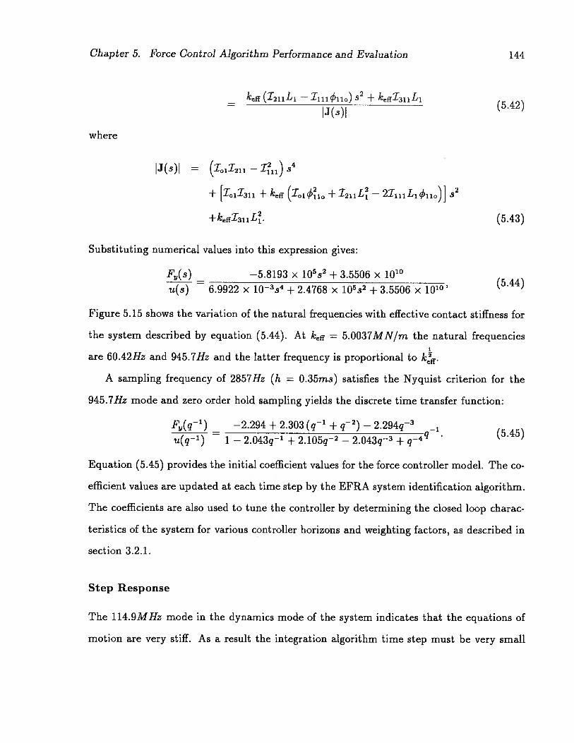
Chapter 5. Force Control Algorithm Performance and Evaluation 144
keff (1211L1— Ii&i) 52 + keffI3llL1
5 42
where
(1011211 — I2) 4
+ [1011311 + keff +I211L —2I111L1110)}2
+keffI3llL. (5.43)
Substituting numerical values into this expression gives:
Fr(s) — —5.8193 x 10⁵s2 + 3.5506 X 10u(s) — 6.9922 x 10s + 2.4768 x 10⁵s2 + 3.5506 x 10¹⁰’ ( . )
Figure 5.15 shows the variation of the natural frequencies with effective contact stiffness for
the system described by equation (5.44). At keff = 5.0037MN/m the natural frequencies
are 60.42Hz and 945.7Hz and the latter frequency is proportional to kff.
A sampling frequency of 2857Hz (h 0.35ms) satisfies the Nyquist criterion for the
945.7Hz mode and zero order hold sampling yields the discrete time transfer function:
F(q’) — —2.294 + 2.303 (q + q2) — 2.294q3 —1 (5 45)u(q’) — 1 —2.043q’ + 2.105q2 —2.043q3+
q4
Equation (5.45) provides the initial coefficient values for the force controller model. The co
efficient values are updated at each time step by the EFRA system identification algorithm.
The coefficients are also used to tune the controller by determining the closed ioop charac
teristics of the system for various controller horizons and weighting factors, as described in
section 3.2.1.
Step Response
The 114.9MHz mode in the dynamics mode of the system indicates that the equations of
motion are very stiff. As a result the integration algorithm time step must be very small

Chapter 5. Force Control Algorithm Performance and Evaluation
10 —
102 101 j2 iøEffective Contact Stiffness [kN/m]
Figure 5.15: Variation of natural frequencies of a single flexible link (with one structuralmode) in contact.
145
k =5.0037MN/moff
I I II
ff=61.55N/rn:
>‘0
a)Dc,.
U(0L..D
z
I I iiiiiil I I iiiiiil I I 111111 I I I 1111111 I I I IIIII

Chapter 5. Force Control Algorithm Performance and Evaluation 146
N2 N Overdamped Mode Underdamped ModeDominant Pole fd [Hz] C
18 1 -45.21 857.5 0.30420 2 -96.76 1429 0.35919 3 -84.38 1429 0.56221 4 -99.13 1429 0.239
Table 5.4: Stabilising controller horizons and closed loop characteristics for steel on aluminium contact (keff = 5.0037MN/m) for a single flexible link with one structural mode.fd = damped natural frequency and (= damping ratio.
and long run times are expected. Figure 5.16 shows the initial 12.5ms of a step response
which required 50.3 hours of CPU time to calculate on a Sun SparcStation 2. Also shown is
the response calculated using a steady state approximation of the contact dynamics which
required only 23.2s of CPU time. The results are almost indistinguishable and hence it is
concluded that, under conditions when the contact dynamics mode is well separated from
the other modes of the system, the contact dynamics can be approximated by their steady
state response with substantial savings in computation time and negligible difference in the
computed results.
Using equation (5.45) and the expression for the closed loop transfer function derived
in section 3.2.1, four combinations of prediction horizon (N2) and control horizon (Ne)
which yield stable control were identified. They are listed, with corresponding approximate
continuous time domain closed loop characteristics, in Table 5.4. In all four cases the closed
loop is characterised by one overdamped mode (a pair of poles on the negative real axis)
and one underdamped mode (a complex conjugate pair of poles in the left half plane).
The natural frequency and damping ratio of the underdamped mode are such that its
oscillation disappear long before the response, dominated by the smaller magnitude pole
of the overdamped mode, reaches the setpoint. Figure 5.17 shows the step response of the
adaptive predictive force controller with N2 = 20, N,, = 2, ), = 0, and .Xse = 0. The
response shown starts from a stable 5N contact force level in order to focus on the step

Chapter 5. Force Control Algorithm Performance and Evaluation 147
I I I I I I
3.2
______
Steady State3.0 - Approximation
2.8FuliContact
2.6:I
2.4 -
2.2 -
2.0 -
ci) -
C.)
C -
1.6 -
8 1.4 -
1.2 -
1.0 -
.8 -
.4 -
.2 -
0 ‘ I I I I I0 .001 .002 .003 .004 .005 .006 .007 .008 .009 .010 .011 .012 .013
Time [SI
Figure 5.16: Comparison of results from simulations using full contact dynamics and steadystate approximation.

Chapter 5. Force Control Algorithm Performance and Evaluation 148
22
20
18
16
14
z12
1000
8
6
4
2
00 .02 .04 .06 .08 .10 .12 .14 .16 .18 .20 .22 .24 .26 .28 .30 .32
Time [s]
Figure 5.17: Force control step response for a single flexible link (with one structural mode),steel on aluminium contact (ken = 5MN/m) with N2 = 20, N = 2, ) = 0, and ‘se 0.

Chapter 5. Force Control Algorithm Performance and Evaluation 149
response performance of the controller and avoid the complications due to the discontinuity
in the system dynamics which occurs at ON as contact is initiated. Control through the
discontinuity is discussed in section 5.4.
The N2 = 20 and N = 2 combination of horizons offers the best compromise of rise time
and control signal activity. The rise time is related to the magnitude of the dominate closed
loop pole. The closer that pole is to the origin (in the continuous time domain), the longer
the rise time. The rise times achieved with N = 1 and N 3 are both longer than that
with N = 2 and, while the rise time with N = 4 is less than with N 2, the control input
signal becomes excessively active and subject to ringing. In all cases prediction horizons
less than those in Table 5.4 yield an unstable closed ioop and increasing N2 causes the slow
mode to become slightly underdamped, introducing overshoot into the response.
Increasing the control increment weighting factor, , from zero has negligible effect on
the response because the closed ioop poles introduced by are generally close to the origin
in the discrete time domain or they interact with the poles of the fast mode; in either case
the slow mode remains dominant.
Figure 5.18 shows superimposed step response simulations for ‘\se ranging from 0 to
0.4. As .kse is increased the rise time decreases but at the expense of increasing overshoot,
which may be undesirable. It is evident from these observations that the static equilibrium
bias term in the control law acts as a proportional feedforward term in which the gain is
proportional to se
The inherent tendency of the predictive controller to anticipate changes in the setpoint
level is apparent in the step responses shown. With a 20 step prediction horizon and
O.35ms sampling interval the controller begins to respond to setpoint changes 7ms before
they occur. The initial sign of the response to a step change in setpoint is opposite to that
of the step due to the nonminimum phase nature of the system dynamics.

Chapter 5. Force Control Algorithm Performance and Evaluation
zC)0U
0
0C)
Time [s]
Figure 5.18: Force control step responses for a single flexible link (with one structuralmode), steel on aluminium contact (keff = 5MN/m) with 0 A3e 0.4.
150
18
16
14
12
10
8
6
4
2
00 .01 .02 .03 .04 .05 .06 .07 .08 .09

Chapter 5. Force Control Algorithm Performance and Evaluation 151
5.3.5 ke = 62kN/m Contact Stiffness Case
The sampling rate of nearly 3kHz required to obtain the results shown in section 5.3.4
means that implementation of the controller would require very high performance hardware
and actuators. The high sampling rate is required because the effective contact stiffness
of 5MN/m is very much greater than the 7096N/m modal stiffness of the link and thus
the dynamics are dominated by the high frequency mode whose natural frequency is pro
portional to k!ff as can be seen in Figure 5.15. Inclusion of additional structural modes in
the dynamics and controller models results in a dominant mode with even higher natural
frequency and thus higher sampling requirements. However, it must be recalled that the
Hertz contact model used to determine the contact stiffnesses and masses is based strictly
on the local deformations of the surface during quasi-static contact. An, et al. [141 used a
parameter estimation algorithm to determine experimentally the effective contact stiffness
of a steel bearing on an aluminium surface and found it to be 61554N/m. Unfortunately
sensor limitations prevented the determination of effective mass and damping coefficients
from their experimental data. It can be surmised that, while the local effective contact
stiffness of a pair of surfaces may approach that given by the Hertz model, more global
deformation of the bodies results in much lower actual effective contact stiffnesses. This
proposition is somewhat supported by the presence of an initial spike in the data collected
by An, et al. (reproduced as Figure 5.19) which suggests that the contact stiffness upon
initial contact is much greater than that which prevails once contact is well established.
Controller Model
To obtain an effective contact stiffness of 61554N/m the values in Table 5.3 were scaled
to maintain relative stiffnesses of the steel and aluminium surfaces with the result that
the steel surface stiffness becomes k3 2.3930 >< 105N/m and that of the aluminium k =

Chapter 5. Force Control Algorithm Performance and Evaluation 152
IC 800007000060000soooo Final Value: 61554 N/rn40000300002000010000
00.0 0.2 0.4 0.6 0.8 1.0
Estimated Stiffness [or Aluminum Surface (N/rn)
Figure 5.19: Experimental contact stiffness estimate for steel on aluminium. Reproducedfrom An, et al. [14]
8.2870 x 10⁴N/m. As can be seen in Figure 5.15, these values imply that, in contrast to
the situation at higher effective contact stiffness, the system characteristics are composed of
contributions from both modes. The natural frequencies of the open ioop modes are 50.65Hz
and 125.0Hz, thus sampling at 384.6Hz (h 2.6ms) satisfies the Nyquist criterion. The
resulting discrete time transfer function model for the controller is:
F(q1) — —2.144 + 3.084 (q1 + q2) — 2.144q3 —1 (5 46)u(q1) 1 — 0.4456q1+ 0.7709q2 —0.4456q3+q_4
Step Response
The approximate closed ioop poles, calculated from the control law and the linearised system
dynamics, show that for N,. = 1 and N,. = 2 all values for the prediction horizon result
in both of the closed ioop modes being uriderdamped. With a 3 step control horizon the
approximate closed ioop poles show that for certain prediction horizons the closed ioop
system has one overdamped mode and one underdamped mode, otherwise both modes are
underdamped. With N,. = 4 there is always one overdamped and one underdamped closed
loop mode. Table 5.5 lists the approximate closed ioop characteristics of the system for
several combinations of prediction and control horizon.

Chapter 5. Force Control Algorithm Performance and Evaluation 153
N2 N Overdamped Mode Underdamped ModeDominant Pole fd [Hz] C
5 3 -181.3 192.3 0.2007 3 -99.07 192.3 0.3218 3 -58.56 192.3 0.342
10 3 -190.1 192.3 0.4115 4 -183.7 192.3 0.1426 4 -171.4 192.3 0.1667 4 -79.75 192.3 0.2898 4 -44.51 192.3 0.3019 4 -80.90 192.3 0.312
10 4 -75.68 192.3 0.314
Table 5.5: Stabilising controller horizons and closed ioop characteristics for steel on aluminium contact (keff = 61.554kN/m) with a single flexible link with one structural mode.fd damped natural frequency and C = damping ratio.
The dominant pole locations and damping ratios listed in Table 5.5 suggest that the
N2 10, N = 3 controller will provide the fastest rise time combined with the least 192.3Hz
disturbance. As Figure 5.20 shows, this is indeed the case, however this performance comes
at the expense of the controller adjusting the system well in advance (26ms) of setpoint
changes because of the 10 step prediction horizon. This potentially undersirable anticipation
effect is markedly reduced with N2 5 and N, = 4 without much increase in rise time but
the response exhibits slight overshoots due to the low damping of the 192.3Hz mode (see
Figure 5.21). The next best set of controller horizons is N2 = 5, Ne,, = 3 which produces the
response shown in Figure 5.22. The rise time of this response is slightly greater than that of
the two previous ones but the 192.3Hz mode is sufficiently well damped to avoid overshoot
and the setpoint change anticipation time is limited to l3ms. These results emphasise the
need for simulations in the tuning of the controller due to the approximate nature of the
closed ioop characteristics calculated based on linearised models, and to the fact that those
characteristics reveal nothing about the relative excitation levels of the closed loop modes.

Chapter 5. Force Control Algorithm Performance and Evaluation 154
20
18
16
14
z12C)0U
100C)
8
6
4
2
Time [s]
Figure 5.20: Force control step response for a single mode flexible link (with one structuralmode), steel on aluminium contact (keff = 61.554kN/m) with N2 10, N = 3, = 0,‘se =
0 .02 .04 .06 .08 .10 .12 .14 .16 .18 .20 .22 .24 .26 .28 .30 .32

Chapter 5. Force Control Algorithm Performance and Evaluation 155
22
20
18
16
14z00
IL 12C)
C0
10
8
6
4
20 .02 .04 .06 .08 .10 .12 .14 .16 .18 .20 .22 .24 .26 .28 .30 .32
Time [s]
Figure 5.21: Force control step response for a single mode flexible link (with one structuralmode), steel on aluminium contact (keff 61.554kN/m) with N2 5, N = 4, = 0,‘se 0.

Chapter 5. Force Control Algorithm Performance and Evaluation
20
18
16
14
z12
C.)
0U
C.)Cu
1000
8
6
4
2
156
0 .02 .04 .06 .08 .10 .12 .14 .16 .18 .20 .22 .24 .26 .28 .30 .32
Time [s]
Figure 5.22: Force control step response for a single flexible link (with one structural mode),steel on aluminium contact (keff = 61.554kN/m) with N2 5, N = 3, \ = 0, ‘\se 0.

Chapter 5. Force Control Algorithm Performance and Evaluation 157
Table 5.5 indicates a potential difficulty with the 3 step control horizon in that the
closed ioop system does not always have an overdamped mode. This implies a possible
lack of robustness in that the effects of unmodelled dynamics or sensor noise may cause
the estimated controller model coefficients to change such that controller horizons which
initially provided an overdamped closed loop mode would no longer do so. For this reason
the 4 step control horizon is preferable. Figure 5.23 shows step responses for the controller
with N2 = 7 and N = 4. The responses are free of overshoot and steady state offset with
a rise time of 24ms.
It can be seen from Table 5.5 that the closed ioop characteristics do not vary mono-
tonically with the controller horizons. This is due to the fact that the horizons are integer
multiples of the sampling interval, h, and this results in an aliasing effect.
We now consider the effect of additional structural modes in the link model. Figure 5.24
shows the natural frequencies of the linearised equations of motion for the single link system
with the link structure modelled by the first three mode shapes of a cantilever beam. At
keff = 61.554kN/m the open ioop natural frequencies are 37.49Hz, 113.5Hz, 231.5Hz and
664.9Hz. It is evident from Figure 5.24 that the frequencies of the latter two open loop
modes which arise due to the additional admissible functions are independent of keff
Under these circumstances the results of section 5.2.2 imply that the additional modes
make minimal contribution to the contact force and thus the sampling rate need not be
increased to resolve them. On the other hand, the control input channels energy into all of
the modes and so they should be included in the controller model. The result of theses two
conclusions is the controller model
F,(q1) —
ui(q’) —
—0.41 — 1.43q’ + 2.56q2 + 3.08(q3+ q4) + 2.56q5 — 1.43q6 — 0.41q71 + 0.79q’ + l.50q2 + 0.21q3 + O.64q4+ O.21q5+ 1.50q6 + 0.79q7+
q_8
(5.47)

Chapter 5. Force Control Algorithm Performance and Evaluation 158
20
18
16
14
12zci,
F:6
4
2
00 .02 .04 .06 .08 .10 .12 .14 .16 .18 .20 .22 .24 .26 .28 .30 .32
Time [s]
Figure 5.23: Force control step response for a single flexible link (with one structural mode),steel on aluminium contact (keff = 61.554kN/m) with N2 = 7, N1, = 4, A, = = 0

Chapter 5. Force Control Algorithm Performance and Evaluation
I 11111111 I I
159
I I I I liii I I I I I 1111 I I I I I I 1——I-—I—1—i•
k = 61 554 kN/m
-icr
>‘()Ca,zwU
(15I.
D
z
108
1
iø
iø
1
11
1 ø
-+--------
I iiiiiil I I 1111111 I I iiiliiil I iiiiiil 1 111111
iø iø 101 102 iø
Effective Contact Stiffness [kN/m]
Figure 5.24: Variation of the natural frequencies of a single flexible link (El1 = 574N mwith three structural modes) in contact.

Chapter 5. Force Control Algorithm Performance and Evaluation 160
Overdamped Mode 192.3Hz Mode Underdamped ModesN2 N Dominant Pole C fd [Hz] C f [Hz] C6 4 -217.5 0.517 105.5 0 192.3 0.3077 4 -157.8 0.584 105.3 0 149.4 0.2018 4 -105.8 0.624 105.3 0 145.0 0.1229 4 -81.56 0.622 105.3 0 151.5 0.140
10 4 -53.99 0.638 105.3 0 143.5 0.125
Table 5.6: Stabilising controller horizons and closed ioop characteristics for steel on aluminium contact (keff = 61.554kN/m) with a single flexible link with three structural modes.fd = damped natural frequency and C = damping ratio.
in which the two high frequency modes are aliased to 153.1Hz and 104.3Hz due to the
relatively low sampling rate. The aliasing of these modes presents little difficulty because
of their minimal excitation.
Table 5.6 lists the approximate closed loop characteristics calculated from the linearised
model of the system for several prediction horizon values with a control horizon of N = 4.
As in the previous cases, the closed loop response is composed of an overdamped mode, the
smallest magnitude pole of which defines the rise time, and an underdamped mode with a
natural frequency of one half the sampling frequency. In addition, the aliased high frequency
modes appear as lightly damped modes in the closed loop. Simulated step responses show
that, as was observed in the case of the one mode link, the fast rise times produced by short
prediction horizons (N2 = 6, 7) are accompanied by overshoot because the underdamped
modes do not die out sufficiently before the response reaches the set point level. Figure 5.25
shows the response with N2 8 which is free of overshoot.
5.3.6 Summary
In summary, this section has illustrated the calculation of the parameters of the link, contact
and controller models based on the physical dimensions and material properties of particular
physical systems. The link model was based on a 1.Om long, 2.0cm diameter aluminium

Chapter 5. Force Control Algorithm Performance and Evaluation 161
22
28
18
16
14
z12
.100
C.)
8
6
4
2
80 .02 .04 .06 .08 .10 .12 .14 .16 .18 .20 .22 .24 .26 .28 .30 .32
Time [SI
Figure 5.25: Force control step response for single flexible link (with three structural modes),steel on aluminium contact (keff 61.554kN/m), with N2 8, N = 4, = 0, . = 0.

Chapter 5. Force Control Algorithm Performance and Evaluation 162
rod with its structural dynamics modelled using the mode shape functions of a cantilever
beam. For the case of relatively soft (kff = 3100N/m) contacting surfaces, with excitation
of the contact dynamics due to the contact mass being significant compared to the link
moment of inertia, simulation results demonstrate stable control with fast rise time and
minor overshoot.
Contact model parameters calculated from the Hertz contact model (derived in sec
tion 2.5), based on a 4.0mm diameter steel bearing as an end effector on the link contacting
a planar aluminium surface, resulted in very stiff contacting surfaces (keff 5.0037MN/m).
The calculation of the closed ioop response of this system was found to be very time consum
ing due to the mathematically stiff structure of the equations of motion, however a steady
state approximation of the contact dynamics portion of the model was shown to substan
tially reduce the computation time without significantly affecting the results. Approximate
closed loop characteristics calculated from the controller model and the linearised equations
of motion were successfully used to tune the controller for the case of a one mode flexible
link. However, control of this system requires 2857hz sampling and the effective contact
stiffness is so much greater than the link structural stiffness that, for any reasonable number
of admissible functions used to model the link structure, the dynamics are dominated by
the highest frequency mode and an even higher sampling rate is necessary.
Experimental results from An, et al. [14] suggest that the effective contact stiffness of
5.0037MN/m given by the Hertz contact model is an extreme upper bound and that a more
reasonable value is keff = 61.554kN/m. At this level of effective contact stiffness the system
was found to be dominated by the two modes with the lowest natural frequencies, as the
results of the linear analysis in section 5.2.2 suggest should be the case. The approximate
closed loop characteristics, calculated from the control law and the linearised system model,
are used to select stable, robust controller parameters for the case of the link structure
modelled by a single admissible function.
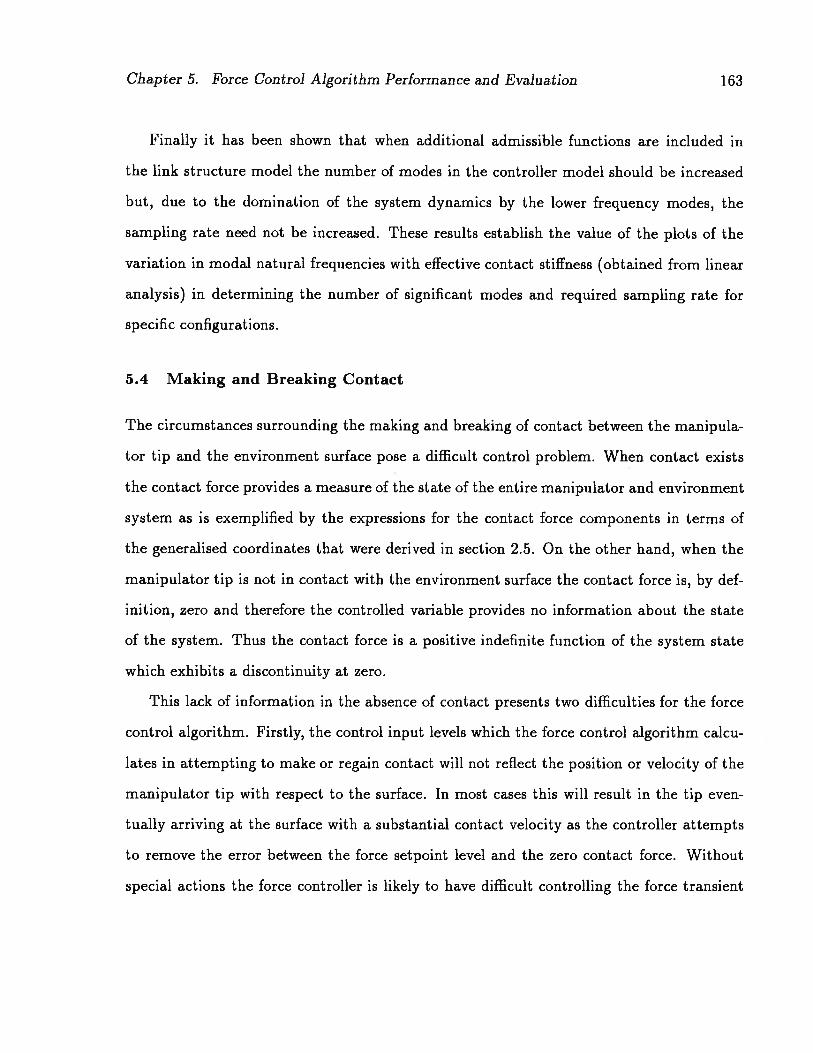
Chapter 5. Force Control Algorithm Performance and Evaluation 163
Finally it has been shown that when additional admissible functions are included in
the link structure model the number of modes in the controller model should be increased
but, due to the domination of the system dynamics by the lower frequency modes, the
sampling rate need not be increased. These results establish the value of the plots of the
variation in modal natural frequencies with effective contact stiffness (obtained from linear
analysis) in determining the number of significant modes and required sampling rate for
specific configurations.
5.4 Making and Breaking Contact
The circumstances surrounding the making and breaking of contact between the manipula
tor tip and the environment surface pose a difficult control problem. When contact exists
the contact force provides a measure of the state of the entire manipulator and environment
system as is exemplified by the expressions for the contact force components in terms of
the generalised coordinates that were derived in section 2.5. On the other hand, when the
manipulator tip is not in contact with the environment surface the contact force is, by def
inition, zero and therefore the controlled variable provides no information about the state
of the system. Thus the contact force is a positive indefinite function of the system state
which exhibits a discontinuity at zero.
This lack of information in the absence of contact presents two difficulties for the force
control algorithm. Firstly, the control input levels which the force control algorithm calcu
lates in attempting to make or regain contact will not reflect the position or velocity of the
manipulator tip with respect to the surface. In most cases this will result in the tip even
tually arriving at the surface with a substantial contact velocity as the controller attempts
to remove the error between the force setpoint level and the zero contact force. Without
special actions the force controller is likely to have difficult controlling the force transient

Chapter 5. Force Control Algorithm Performance and Evaluation 164
which results from a non-zero contact velocity. The second difficulty arises in the operation
of the system identification algorithm used in the adaptive controller because the algorithm
updates the model coefficients on the basis of the difference between the actual and pre
dicted output with the tacit assumption that the model and the system being identified are
continuous through zero.
In order to overcome these difficulties it is necessary to control the motion of the manip
ulator when it is not in contact as well as the forces it exerts on the surface when it is. The
predictive control algorithm derived in Chapter 3 can be readily applied to the task of con
trolling the manipulator joint angles simply by providing it with a transfer function model
which relates the joint angles to the control inputs. To successfully use the combination of
force and motion controllers to operate through the discontinuity when contact is made or
broken a level of control above the basic predictive control algorithm is introduced. This
higher level control is referred to as the Contact Control Logic. Like the circumstances it
is intended to deal with, it is discontinuous and, to some extent, heuristic in nature. On
the basis of sensor inputs and data supplied by the operator and the trajectory generator
the contact control logic generates the setpoint programs for the predictive control algo
rithm, selects between force and motion control algorithms and chooses whether or not to
allow system identification to proceed. The relationship of the contact control logic to the
manipulator, sensors and other elements of the control structure is shown in Figure 5.26.
The contact events which must be dealt with by the contact control logic can be broadly
classified as expected (or intentional) and unexpected. An example of an intentional contact
event is the situation where the operator or task planner accurately knows the location of
the surface to be contacted. Under these circumstances motion control can be used to
move the manipulator tip to a location adjacent to the surface and to reduce its approach
velocity sufficiently to avoid a violent collision and accompanying high level of transient
contact force. From this state a smooth transition to force control can be made. The role

Chapter 5. Force Control Algorithm Performance and Evaluation 165
Figure 5.26: Block diagram of the overall control structure.

Chapter 5. Force Control Algorithm Performance and Evaluation 166
of the contact control logic in this situation is to switch between motion and force control
at the appropriate time as directed by the operator or task planner.
In contrast, an example of an unexpected contact event is the situation when, due to
imperfect knowledge of the manipulator’s working environment, it collides with a surface.
If the collision is due to an object being unexpectedly in the path of manipulator motion
the contact control logic must take measures to minimise the collision force and bring the
manipulator to rest, pending corrective action from the operator or task planner. On the
other hand, if the collision is due to inaccurate knowledge of the location of a surface on
which the manipulator was intended to exert force the role of the contact control logic is
to switch to force control mode, minimise the force transient that results from the collision
and reach the desired force level setpoint. This latter case is the focus of the remainder
of this section. Two operational strategies for the contact control logic which seek to
achieve sustained, controlled contact force control following an unexpected contact event
are proposed and their performance is examined by way of simulations. The analysis, results
and discussion presented in this section have already been published [27].
5.4.1 Stop Motion Strategy
The first, relatively simple, strategy is referred to as the stop motion strategy. The contact
control logic is programmed such that the control mode is switched from motion to force
when a non-zero contact force is sensed and motion control is resumed if contact is broken.
In addition, when contact occurs the motion control setpoint is changed so that when the
motion controller resumes operation, rather than continuing the with motion that that
was being executed prior to contact, the joint angles at which contact was made will be
maintained.
Figure 5.27 shows the results of a simulation in which this strategy is used. A single
link manipulator is used, modelled on a 1Mm long, 2.0cm diameter aluminium rod with the

Chapter 5. Force Control Algorithm Performance and Evaluation
20
i:; 150Co 100
(b) Contact Force Response
167
Figure 5.27: Joint angle and contact force responses for a single flexible link colliding with a6200N/m surface. Control mode switching is based on sensed contact force and the motioncontrol setpoint is modified due to the contact event.
(a) Joint Angle Response
30
Time [sJ

Chapter 5. Force Control Algorithm Performance and Evaluation 168
structural dynamics represent by the first two modes of the rod considered as a cantilever
beam. The link is initially in motion with constant joint velocity toward a surface with
a contact stiffness of 6200N/m. The predictive control algorithm parameters are a delay
horizon (N1) of 1 time step, a prediction horizon (N2) of 40 time steps, a control horizon
(Na) of 12 time steps and a control increment weighting factor () of 1.0. The controller
time step is 4.Oms. The motion controller is adaptive but the model coefficients for the force
controller are held constant. A non-adaptive (i.e. fixed model coefficients) force controller
has been used in order to focus attention of the issues surrounding the transition from
motion to force control. The problems that arise when adaptive force control is used during
this transition period are discussed below.
The simulated joint angle and contact force responses (solid lines) and corresponding
setpoints (dashed lines) are shown in Figures 5.27a and 5.27b, respectively. The motion
controller shows good tracking of the joint angle ramp during the initial part of the maneu
ver. The desired angular velocity of the joint is 0.5rad/s which gives a nominal velocity at
the link tip of O.5m/s (neglecting the vibrational motion of the flexible link). After 0.257s
the link tip contacts the environment surface with a velocity of 0.536m/s. At this point
the control mode is switched from motion to force due to the sensing of a non-zero contact
force and the force controller attempts to bring the system to rest at the specified contact
force setpoint of 8.ON. Upon switching control modes the motion control setpoint for future
use is modified to hold the joint angle stationary at 7.56°, the joint angle at which contact
was detected. Due to the non-zero velocity of the link tip at the instant of contact the
contact force rises rapidly to approximately 16N and, before the force controller can have
any significant effect on the system the link rebounds from the surface and motion control
is resumed. This cycle is repeated twice more with force control being established on the
third contact.

Chapter 5. Force Control Algorithm Performance and Evaluation 169
After sustained contact has been achieved an adaptive force controller (i.e. one for which
the model coefficients are updated using a system identification algorithm at each time step)
is the correct choice. However a non-adaptive controller (i.e. fixed model coefficients) is
required during the transition period while the tip is bouncing on the environment surface.
During this period the brief intervals of rapidly changing force levels interspersed with
periods of zero force cause the system identification algorithm to produce wildly inaccurate
estimates of the model coefficients. Using these coefficients in the control law can result in a
loss of control. A solution to this problem is to delay the start of force model identification
until sustained contact is assured. A delay of 25 time steps is adequate for the case shown
in Figure 5.27. However, this approach requires that some means be devised to decide
that sustained contact has been achieved; a difficult proposition considering the number of
factors on which the duration of the transition period (number of bounces) depends.
In addition to the difficulties involved in using adaptive force control during the transi
tion period, the strategy of bouncing on the surface until force control can be achieved is, for
most applications, not acceptable. Furthermore, it has been observed in other simulation
runs that the number of bounces can be much greater than the three seen in Figure 5.27b,
depending on the dynamic characteristics of the link and the surface. Worst of all, there
is, apparently, no guarantee that stable force control will in fact be achieved at all using
this strategy. While various refinements of the motion control strategy during the bounces
might produce better results, observation of the contact force transient which occurs during
the first bounce suggests another course of action.
5.4.2 Force Setpoint Modification Strategy
Comparison of the contact force transient during the first period of contact in Figure 5.27b
with the corresponding transient for a collision between the link and the environment at the
same velocity during which no attempt is made to control the contact force shows very clear

Chapter 5. Force Control Algorithm Performance and Evaluation 170
Figure 5.28: Simple 1 degree of freedom model of a single link in contact with an environment.
similarity between the transients. In both cases the transient closely resembles the positive
portion of a sinusoid, the period of which correlates closely with the natural frequency of
the first mode of the open loop system. Based on this observation it is apparent that the
force controller has almost no effect on the contact force level immediately following contact
and that the response of the system at that time is entirely due to the open ioop dynamics,
in particular the velocity of the link at the instant of contact.
This suggestion is confirmed by consideration of the simple single degree of freedom
model of the link and contact dynamics shown in Figure 5.28. The equation of motion of
this system without forcing is
I8 + kL28 = 0 (5.48)
Given initial conditions at t = 0 of 8 = 0 and & =&, the particular solution of equation (5.48)
iskL2
8(t) = —sinwt, wherew2 =
10k
/
Li.)(5.49)

Chapter 5. Force Control Algorithm Performance and Evaluation 171
In this model the contact force is the force generated by the compression of the spring, that
is
F(t) = kLO(t)
kL8sinwt
w
= Fksinwt, (5.50)
where Fk=
With Ic set to the value of the effective stiffness of the link and environment surfaces
(considered in series) and 10 set equal to the rigid body moment of inertia of the link
about the joint axis, equation (5.50) gives a very good prediction of the initial contact force
transient shown in Figure 5.27b.
Note that the contact force transient described by equation (5.50) is entirely a result of
the initial condition velocity, which correlates with to the velocity with which the link tip
contacts the surface. The classical form of transfer function model on which the predictive
force control algorithm is based, however, assumes quiescent initial conditions (that is, the
system is stationary at the instant of contact). Thus, a fundamental incompatibility exists
between the system for which control is desired and the model on which the controller is
based.
Viewing the situation in terms of energy, the force controller expects the system to have
zero energy when it begins operation. The system however has non-zero energy, in the
amount of the kinetic energy of the link at the instant of contact. If stable force control is
to be achieved without letting the link bounce off the surface the controller must overcome
the initial energy of the system. This is confirmed by simulations similar to those shown
in Figure 5.27, in which higher contact force setpoints are specified. In those simulations
the initial portion of the contact force transient is similar to the corresponding uncontrolled
collision transient, however the force controller (which is more energetic by virtue of the
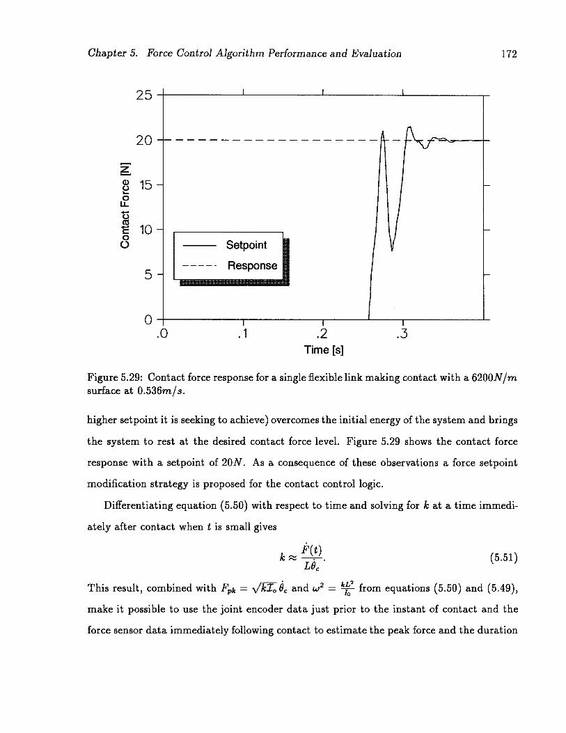
Chapter 5. Force Control Algorithm Performance and Evaluation
z0C.)0I]4.-C-)(U4.-
0C-)
172
.0 .1 .2 .3
25
20
15
10
5
0
Time [s]
Figure 5.29: Contact force response for a single flexible link making contact with a 6200N/msurface at 0.536m/s.
higher setpoint it is seeking to achieve) overcomes the initial energy of the system and brings
the system to rest at the desired contact force level. Figure 5.29 shows the contact force
response with a setpoint of 20N. As a consequence of these observations a force setpoint
modification strategy is proposed for the contact control logic.
Differentiating equation (5.50) with respect to time and solving for k at a time immedi
ately after contact when t is small gives
1(t)k —v—-. (5.51)
L6
This result, combined with Fk = /J6 and w2=
from equations (5.50) and (5.49),
make it possible to use the joint encoder data just prior to the instant of contact and the
force sensor data immediately following contact to estimate the peak force and the duration

Chapter 5. Force Control Algorithm Performance and Evaluation 173
20
15
zci)C)
10
C0
C)
5
0
Time [sj
Figure 5.30: Contact force response of a single flexible link colliding with a 6200N/m surfacewith force setpoint modification.
() of the contact that will occur if the force controller does not act. The peak force is
effectively a measure of the initial energy of the system which the controller must overcome.
In order to do this the specified setpoint is compared to the estimated peak force. If the
setpoint is found to be less than the estimated peak the former is modified to the estimated
peak force level for a period of time equal to predicted duration of the uncontrolled collision
contact transient. This enables the controller to exert the energy necessary to overcome the
initial kinetic energy of the link.
Figure 5.30 shows the contact force response for the same conditions as that shown in
Figure 5.27 but with contact transient prediction and contact force setpoint modification
included in the contact control logic. Contact occurs at 0.257s with a link tip velocity of
.0 .1 .2 .3

Chapter 5. Force Control Algorithm Performance and Evaluation 174
0.536m/s. At 0.260s the force controller estimates the effective stiffness of the contactingsurfaces to be 3041N/m (compared to the actual value of 3100N/m) and predicts a peak
force of 15.69N and an uncontrolled contact duration of 30.2ms. Based on these predictionsthe contact force setpoint is raised to 15.69N for 30.2ms and a stable 8.ON contact force
level is achieved without the link leaving the surface as happened in Figure 5.27b. The initial
overshoot in Figure 5.30 is largely due to the initial contact velocity of the link and cannotbe removed by a controller which has no provision for non-zero initial conditions. In anycase, the overshoot is significantly less that that which eventually occurs in Figure 5.27b.
The model, based on equation (5.50), used to predict the peak contact force and cor
responding uncontrolled contact duration is a very simple one. The necessary calculations
require a total of 2 additions, 5 multiplications and 2 square root operations. (Two ad
ditions and one multiplication can be eliminated from this total if the force rate can be
obtained from the force sensor.) As such, the setpoint modification can easily be put into
effect within one or two time steps after contact is sensed. Furthermore, it has been noted
in simulation results that a lag of one or two sampling intervals between the instant of
contact and the completion of the prediction calculation (and application of the setpoint
modification) does not adversely effect the control.
5.5 Force Control for Two Link Manipulators
Consideration of a manipulator with two or more links greatly increases the complexity of
the analysis and control problems. In this section force control for planar manipulators with
two links is addressed. Both rigid link and flexible link manipulators are considered. The
two joint torques available as control inputs for a two link manipulator permit control of
two world frame components of contact force.

Chapter 5. Force Control Algorithm Performance and Evaluation 175
In this what follows, similar analytical techniques to those used in section 5.2 are em
ployed to gain insight into the modal structure of the system and the results are applied
to the selection of appropriate controller parameters. Because of the strongly coupled na
ture of the system the multivariable control algorithm is necessary. The derivation of an
appropriate multivariable controller model from the linearised equations of motion is pre
sented. Simulated step responses are used to evaluate the performance of the closed loop
force control for both rigid link and flexible link manipulators.
5.5.1 Linear Analysis
In this section a linear analysis of a two link manipulator in contact with a deformable en
vironment is presented. The analysis follows the same general approach that was employed
for a single link system in section 5.2.
Rigid Links
We begin by considering the case of rigid links which is the limiting case of infinite link
stiffness. As well, the characteristics of rigid link manipulators are of practical interest in
their own right since they typify the vast majority of existing industrial manipulators. Fig
ure 5.31 shows the configuration and important parameters for a manipulator with two rigid
links exerting forces on the environment in the r and y world frame coordinate directions.
The equations of motion for this system are given in section A.2. Neglecting damping,
gravitational effects and inertia coupling between the links and the contact region mass,
replacing the joint torques {Tj(t),r2(t)} with the general control inputs {ui(t),u2(t)} and
linearising about the nominal state
{ B2 Ex Lii x y ] = [ 0 ... 0 j
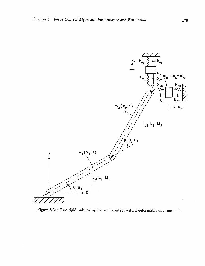
Chapter 5. Force Control Algorithm Performance and Evaluation 176
key
k m5+ me
w2(x2,t)
102 L2 M2
y w1(x1,t)
U2
ILM01 1
x
I
Figure 5.31: Two rigid link manipulator in contact with a deformable environment.

Chapter 5. Force Control Algorithm Performance and Evaluation 177
gives
[101 + 102 + M2 (L +L1L2C) + m (L + L + 2L1L2c)] 1
+ [102 + M2L1L2c + m (L +L1L2c)]
—m [L1.s + L2s2j + m [Lic + L2c2]
= u1(t)— k5 (List + L2s2)[(Ljs + L2s2)Oi + L2s202+ j
—k (Lic + L2c2)[(Lic + L2c2)0 + L2c202—
(5.52)
[I2 + M2L1L2c+ m (L +L1L2c)] i + [102 + mL22] 62
—mL2s2ë+ mL2c2ë
= u2(t)—k3L2s2[(List + L2s2)0 + L2s202+ e]
—k8L2c2[(Lic + L2c2)8 + L2c202— (5.53)
m(Lis + L2s2)8i + mL2s262— më = —k5 [(List + L2s2)0 + L2s282+ e] — kexEx
(5.54)
m (Lic + L2c2)01 + mL2c262+ mi = —k8 [(Lic + L2c2)0 + L2c202—
—
(5.55)
where the generalised coordinates {0, 02, e, e} are now perturbations about the nominal
state.
Figure 5.32 shows the numerically calculated eigenvalues of the system with the following
parameters: 0 = O’, = 90°, 101 = 102 = 0.2817kg m2, M2 = 0.8451kg, L1 = L2 = 1.Om,
and = kex = k8 key. The eigenvalues are shown for the range of effective contact
stiffness, keff, from 50N/m to 5MN/m. As was seen in Figure 5.3, the upper frequency
line in Figure 5.32 is well separated from the other frequencies. That line is actually two
superimposed lines representing the natural frequencies of the contact mass vibration modes

Chapter 5. Force Control Algorithm Performance and Evaluation
1 4
‘Ic’
>‘C)Ca)
a)U-
- 1
z
10’
101 —
1
Effective Contact Stiffness [kN/m]
Figure 5.32: Variation of the natural frequencies with effective contact stiffness for a twolink manipulator with identical, rigid links in contact with an isotropic (kxeff = kyeff) environment.
1 6 I 11111111 I I 1111111 I IIIIII I IIIIIIj I I
113
1/2 1/2
_L rksx÷kexl L ksy+key3 2t Lm+ mej 4 2r [m÷ me
178
14
1 ø
111
.1
101 1 3

Chapter 5. Force Control Algorithm Performance and Evaluation 179
( and 7)4) in the x and y coordinate directions. These lines are closely approximated by
lk+k 2 1 k+kf =
— sX exand f =
— sj ey(5.56)
27r m5 + me 2K m3 + me
They are coincident because k = kex k811 = key for the case shown.
For most cases of practical interest the contact mass is small compared to the other
inertias in the system with the result that the high frequency modes associated with its
local vibration have minimal effect on the rest of the system. As was done in section 5.2.2,
we now introduce a steady state approximation for the contact dynamics and focus the
analysis on the remaining modes. Neglecting the contact region mass, m, and replacing
the directional contact stiffnesses, k8 and kex, k8 and key, with the corresponding effective
contact stiffnesses, kff and kyeff, allows the linearised equations of motion to be reduced
to:
[101 + 102 + M2 (L + LiL2c)] ë1 + [i + M2LiL2c]2
= ui(t) — kxeff (List + L2s2)[(List + L2s2) +L2s2e2]
kyeff (Lic + L2c2)[(Lic + L2c2)8 +L2c282] (5.57)
[102 + M2LiL2cj +
= u2(t) — kffL2s2[(List + L2s2)6i +L2s282j
kyeffL2C2[(Lic + L2c2)&i +L2c282]. (5.58)
After a great deal of algebraic manipulation the characteristic equation for this system
can be written as
+ M2L) 102 — MLLc2] (jw)4
+ [[I +102 + M2 (L + LiL2c)j (k11ff + zks2) L
+102 [kyeff (L + L + 2L1L2c4) + Ak (List +L2s2)2]

Chapter 5. Force Control Algorithm Performance and Evaluation 180
— (2102L2+M2LJ) [kyeff (Lic + L2) + txk (List + L2s2)S2]} (jw)2
+kxeffkyeffLL.32= 0, (559)
where Lik = kxeff — k1jeff. The structure of equation (5.59) provides important insights into
the physical behaviour of the system. Firstly, note that the substitution, kxeff kyeff + 1k,
used to arrive at equation (5.59) separates the overall effects of the contact stiffness from
those due to a difference in the contact stiffnesses in the x and y directions. In particular, this
substitution reveals that the nominal joint angle of link 1, 8, affects the natural frequencies
oniy when kff kyeff. Secondly, in the case of exact alignment of the links (8 00 or
180°), the (jw)° term disappears. This circumstance results in one of the natural frequencies
of the system being zero which implies that the two components of contact force cannot
be simultaneously controlled because the manipulator lacks sufficient degrees of freedom.
This is an analogous situation to the familiar degenerate condition which arises in motion
control when planar links are exactly aligned.
Equation (5.59) can be solved to yield an expression which closely approximates the
natural frequencies of the and 2 modes. For the cases typified by Figure 5.32 (identical
links and keff kyeff keff) we have:
(,w)2
= 2 (z + M2L2)— MLc2 [_ (i + M2L2s2) + (i + ML4s2) 2]. (5.60)
While this expression is somewhat more complex than those obtained in the case of a single
link (equation (5.11)), it displays the came general structure. The natural frequencies
are directly proportional to kff and L and inversely proportional to the square root of a
combination of inertias. This expression also reveals that the frequencies of the and
72 modes vary between bounds as & varies modulo 90°. At 0 = 00 the manipulator
configuration is degenerate and the frequency of ij attains its minimum value, namely zero,
while the frequency of ?)2 is at its maximum. At O = 90° the frequencies are in the ratio

Chapter 5. Force Control Algorithm Performance and Evaluation 181
of 1 to 2 and the frequency of is at its maximum and that of i2 is at its minimum. The
variation if the frequency of i is much larger than that of 72.
Returning our attention to the model which includes the full contact dynamics, we now
consider the eigenvectors of the system and, in particular, the information they provide
about the contributions of the natural modes to the contact force components and the exci
tation of those natural modes by the control inputs. As in the case of a single rigid link, the
eigenvectors, normalised to unit magnitude, are found to be independent of effective contact
stiffness for the case where kxeff = kyeff. With the parameter values used in Figure 5.32 the
eigenvectors are
E [ei e2 e3 e4]
—0.667 —1.286 x 1O_12 —2.962 x iO’ —2.662 x 1O_6
0.667 0.894 1.065 x i0 2.662 x 10⁶(5.61)
8.087 x 10_13 —0.147 1 4.311 x 10u1
0.333 —6.433 x iO’ 1.070 x lO 1
With these numerical values the transformation between the generalised coordinates and
the natural modes of the system,
‘1)1
=ET , (5.62)
174
clearly shows the isolation of the and modes (high frequency vibration of the contact
region mass) from the and 772 modes. The energy of the 772 mode is concentrated in
the oscillation of link 2 about its joint. The h mode includes oscillations of both links
about their joints in equal proportions of opposite sign. This particular arrangement of the
contributions of the 8 and 62 generalised coordinates to the 77i and 772 natural coordinates

Chapter 5. Force Control Algorithm Performance and Evaluation 182
is due to the nominal joint angles, t = 00 and t9 = 90°. The effect on the 7h and 12
eigenvectors of changing the nominal joint angle of the second link is shown in Figure 5.33.
The relatively small contribution of the 8 generalised coordinate to the 2 mode decreases
as increases, as shown in Figure 5.33b. This trend indicates that the majority of the
energy associated with the ‘]2 mode is in the form of oscillations of link 2 about its joint.
Figure 5.33a shows that the i mode combines contributions from 6 and 2 with opposite
signs, reflecting the coupling between the links. The ratio of the components is determined
by the lengths and inertias of the links. In the case shown the links are identical and the
ratio approaches -2 to 1 as the links are aligned and -1 to 1 as they become perpendicular.
The linearised contact force model equations, obtained from equations (2.56) and (2.57)
by neglecting damping and structural flexibility terms, are:
F c2
rhereEs
Eu
= [ - (List + L2s2) -L2s2 (±: - i) o] (5.63)
and
F , where
= k5- [ (Lic + L2c2) L2c2 0 (:: - i) j. (5.64)

\\ \\\\
\I\
)r.
3r..
)
\‘‘
IIIi
iiii
II
\\\\\
c•-
jo
—
\\\\
CC
CC
C
.1
•I
I•
II
•I
I•
cc
Gen
eral
ised
Coo
rdin
ate
Com
pone
nts
ofN
atur
alM
ode
&
Gen
eral
ised
Coo
rdin
ate
Com
pone
nts
ofN
atur
alM
ode
II
II
—
0; CD cz C CD CD
C C0 C
I I1 I I

Chapter 5. Force Control Algorithm Performance and Evaluation 184
Transforming these expression into natural coordinate space we find that, with the eigen
vectors given in equation (5.61),
0 77i
F = —0.4472 772(5.65)
0 773
—5,3248 x 10—6 77
andT
0.3333 77i
F —6.4319 x 10¹³ 772= (5.66)
—1.3312 x 10⁻⁶ 77
—1.4810 x 10_17 77
These results show that the contact forces, F and F, are composed almost entirely of the 772
and 771 modes, respectively, that is, the high frequency vibrations of the contact region mass
contribute minimally to the contact forces. As would be expected from the above discussion
of the natural frequencies, the contact force components in natural coordinate space are
independent of & when Lk = 0. The effect of varying O in the range from 00 to 90° is
shown in Figure 5.34 where the values of the 7i and 712 components of F and F are plotted
for identical links and equal directional contact stiffnesses with keff = 61.554kN/m. When
& is small Figure 5.34b shows that F is dominated by the 772 mode, reflecting the fact that
a motion about joint 2 results primarily in a force in the y direction. For intermediate values
of i9 the motions of both links contribute to F and it is therefore composed of components
of both 77i and 772 At O = 90° the 71i mode dominates F because, in that configuration,
only motion about joint 1 can produce a force in the y direction. The degenerate state
of the manipulator which occurs when the links are aligned is reflected by the zero values
of both the ‘i1 and 72 components of F shown in Figure 5.34b. As éL increases the 772
component increases in magnitude to a maximum at 0 = 90°, in which configuration only

Chapter 5. Force Control Algorithm Performance and Evaluation 185
0
- .05
-.10- 0CLI..
-.15
- 25= a) j2
- .300EZ 8 - .35
- .40
45I I I •
0 10 20 30 40 50 60 70 80 90
o [degrees]
(a) i and 12 components of F
.35
.30
.25
.20
0u .15 /.10
.05
0a) .-
- 05
- 10- 0.0 E -.15Zo
0 - .20
- .25-
. 30
—.35 .• I • • I •
0 10 20 30 40 50 60 70 80 90e [degrees]
(b) and ]2 components of F
Figure 5.34: Variation of the components of F and F in natural coordinate space with 6for identical rigid links with equal directional contact stiffnesses, keff = 61.554kN/m.

Chapter 5. Force Control Algorithm Performance and Evaluation 186
motion about joint 2 can produce a force in the x direction. The i1 component of F is due
to the coupling between the links.
Finally, we consider the relative excitation of the natural modes by the control inputs,
u1 and u2, by using ET to transform the input vectors, [1 0 0 01T and [0 1 0 01T
from generalised to natural coordinate space. As in the single link case, the excitation of
the modes corresponding to the local vibrations of the contact region mass are found to be
negligible when that mass is small compared to the link inertias. The excitations of the
other ( and 1)2) modes are shown in Figure 5.35 for values of éL between 00 and 90°. The
geometric relationships which were discussed above in the context of the contributions of
the 8i and 82 generalised coordinates to the natural modes are reflected in the data shown
in Figure 5.35. The u1 input primarily excites the mode, particularly as the links become
perpendicular. On the other hand, u2, excited both the and the 1)2 modes when the
links are nearly aligned, with the excitation of 1h decreasing somewhat as the links become
perpendicular. The u2 input excites both modes, regardless of the configuration of the
manipulator, because an input at joint 2 not only drives link 2 but also produces a reaction
force on the tip of link 1.
In summary, linear analysis of the contact case for a two link manipulator with infinitely
stiff links under the assumption that the contact region mass is small compared to the link
inertias reveals that:
1. the natural frequencies are proportional to k for a given set of link lengths and
inertias;
2. the natural frequencies of the contact region mass vibration modes (i and ij) are
widely separated from those due to the links oscillating about their joints (‘ii and 1)2);
3. the natural frequencies of the i and 1)2 modes are independent of 6 when kseff = kyeff
and, for a given keff, are bounded above and below as 8 varies modulo 90°;

Chapter 5. Force Control Algorithm Performance and Evaluation
0
- .05
-.10
-.15
.94
.92
.90
.88
.86
.84
.82. x
lii .80LQ)
.78
.76
.74
72
70
.68
.650
Figure 5.35: Relative excitation of thefor a two link rigid manipulator in contact.
187
Caa) .;
o0
. xLu
4-.
U)
11
- .20
- .25
- .30
- .35
10 20 30 40 50
o [degrees]
(a) Joint 1 input, u1
60 70 80 90
10 20 30 40 50 60 70 80
o [degrees]
(b) Joint 2 input, u2
90
7li and 72 modes by the control inputs, u1 and u2,

Chapter 5. Force Control Algorithm Performance and Evaluation 188
4. the contact forces, F and F, are composed primarily of the and 2 natural modes
in proportions which depend on the nominal manipulator geometry; and
5. the control inputs excite only the and 2 modes.
For the purposes of contact force control using a discrete time algorithm these results imply
that the high frequency modes can be ignored and the sampling interval selected to satisfy
the Nyquist criterion for the 2 mode frequency when 8 = 00. Employing the multivariable
form of the predictive control algorithm developed in Chapter 3 with a controller model that
properly includes the effects of coupling (as discussed in section 5.5.2) allows the system to
be easily controlled. The presence of two undamped open loop modes means that a control
horizon of N = 2 is needed. The performance of the force control algorithm for this case
is demonstrated in section 5.5.3.
Flexible Links
The equations of motion for a two flexible link manipulator making contact with a deform-
able environment were derived in Chapter 2 (equations (2.47) through (2.52)). Applying
the steady state approximation for the contact dynamics, linearising about the nominal
manipulator joint angles O = i9 and 62 = 6 (with all other state variables nominally zero),
neglecting damping and gravitational effects, and considering only one flexible mode for
each link, the equations of motion are simplified to:
[r + 102 + M2 (L +L1L2c)] i
+ + M2 (L1 + L2c) &lo + (102 +M2LiL2c)o] ii
+ (102 + M2LiL2c]2 + [1121 +L1cI421]21
— [kff (List +L2s2)2+ kyeff (Lic H- L2c2)2] 81
— [kxeff (s4ii0 +L2s2410)(L1s+ L2s2)+ k,eff (cq.ii0 +L2c2q10)(Lic + L2c2)]‘b

Chapter 5. Force Control Algorithm Performance and Evaluation 189
— [keffL2S2(List + L2s2)+ kyeffL2C2(Lic + L2c2)]82
— [kxeffs2q2lo (List + L2s2)+ kyeffc2qS2lo(Lic + L2c2)] ‘j&21
(5.67)
[im + M2 (L1 + L2c) 11o + (102 + M2L1L2C2)11o] i
*1”+ [I21 + M2 (11O +L2c2&10) + +M2L2c&io) 11
+ [Io21o +M2L2c;iio] 2 + [I12j10+cI42iii0j21
=— {kxeff (sii0 +L2s2q10)(List + L2s2)+ kff (cq110 +L2c2b10)(Lic + L2c2)j 01
— {kxeff (Sii +L2s210)2+ kyeff (c110 +L2c210)2+ 1311] ii
— [kxeff (q11o +L2s2q10)L2s2 + kyeff (cq5iio +L2c2410)L2c2]02
— [kseff (sqiio +L2s2410)S127210 + Icyeff (cqii0 +L2c2410)c2qS210]b21
(5.68)
[102 + M2LiL2c;] i + [1oio +M2L2ciio] ii + I& +
= u2(t) — [kxeffL2S2(List + L2s2)+ kyeffL2C2(Lic + L2c2)jOi
[keffL2S2(sqSii0 +L2s2q10)+k1ieffL2C12(c41i0+L2c24410)jiI)ii
— ceff128l2+ kyeffLC] 02 — [kxeffL2s2s2q!2lo+ kyeffL2C2C242lo]l/’21 (5.69)[k 2*2
[1121 + LicI42i1i + [I1211 +cI421qS110]bi + 112102 + I22121
— [kxeffS24)21o (List + L2s2)+ k,effC22lo(Lic + L2c2)j 81
—[keffs2qS2lo +L2s2q410)+ kyeac2q2io(cq110 +L2c2qS10)1b11
[kxeffs2q21oL2s2+ kyeffCl24)210L2C12]02
*2 i2*2 i2— [kxeffsi2c2io+ kyeffc12q210 + 1321j I’21. (5.70)
Chapter 5. Force Control Algorithm Performance and Evaluation 190
Even in this greatly simplified form an algebraic analysis of the system is difficult to ac
complish as well as to gain insight from. However, the insights obtained through the single
link analysis Section 5.2 and the two rigid link analysis above provide guidance as to the
expected characteristics of the system. These characteristics will be explored numerically.
Figure 5.36 shows the variation in natural frequencies with effective contact stiffness for
a manipulator with identical links, each with a single structural mode, in contact with a
surface having identical contact stiffnesses in the x and y directions. The nominal manip
ulator joint angles are = 00 and 6 = 900. The characteristic pattern of the frequency
lines for the four modes ( through i) with the lowest natural frequencies is recognizably
analogous to the single flexible link case. The pattern implies the same type of transition
seen in the single flexible case, namely domination of the system dynamics at low contact
stiffness by low frequency, rigid link modes (iii and 2) giving way to domination by the
higher frequency, structural modes (m and i) at high stiffnesses. The lines for the 1i and
772 mode natural frequencies are asymptotic to the frequency lines for the corresponding two
rigid link case when the contact stiffness is small. As the effective contact stiffness increases
these frequencies both become independent of keff. The link structural modes each intro
duce a mode (773 and i) whose natural frequency at low contact stiffnesses is independent
of keff while at high stiffnesses the frequency is proportional to kff. The lines for the highest
frequency modes ( and 776) are superimposed in Figure 5.36 because the contact surfaces
are isotropic (keff = kyeff). These modes are the local vibrations of the contact region mass
in the x and y directions.
Other characteristics of the two flexible link system that follow the trends observed in
the earlier linear analyses are:
1. the natural frequencies of the four low frequencies modes are independent of O when
kxeff = kyeff and, for a given keff, they are bounded above and below as O varies

Chapter 5. Force Control Algorithm Performance and Evaluation 191
1 6
N
>C.)
ci)D
I
1 ø
1ø_2 iø
Effective Contact Stiffness [kN/m]
Figure 5.36: Variation of the natural frequencies with effective contact stiffness of a twolink manipulator with identical, flexible (El = 574N m2, one structural mode each) linksin contact with an isotropic (kzeff = kyeff) environment.
1 g_1 1 1gi
1 1

Chapter 5. Force Control Algorithm Performance and Evaluation 192
modulo 900; furthermore, the frequency of the ‘h mode varies over a much larger
range and in opposition to the frequencies of the other modes;
2. additional admissible functions in the link models introduce additional intermediate
frequency modes, each of which dominates the dynamics over a specific range of keff
in a manner analogous that for the single link case shown in Figure 5.10;
3. in the range of contact stiffnesses where they are independent of keff, the natural
frequencies of all but the two highest frequency modes are proportional to the flexural
rigidities of the links;
4. the centres of the ranges of effective contact stiffness values in which the transitions
among dominant modes occur are also proportional to the flexural rigidities of the
links in the same fashion as illustrated in Figure 5.9.
There are two features of particular interest in Figure 5.36 which are not explained
by the linear analyses of the simpler configurations. Firstly, the fact that the and 772
frequency lines both asymptotically approach the same frequency for large values of keff.
This coincidence of frequencies is due to the links having identical lengths and inertias.
Secondly, the curvatures of the and 773 mode frequency lines in the transition range of keff
are somewhat sharper than the curvatures of the 772 and mode lines. This characteristic is
a result of there being, in reality, two overlapping transition ranges. The overlap is also due
to the links being identical. Figure 5.37 shows the situation when link 2 is twice as long and
twice as massive as link 1. The pattern of transfer of dominance from one mode to another
is greatly complicated by the different link lengths but the established characteristics are
still recognisable.
The variation with keff of the contributions of the natural modes to the contact forces
illustrates the affect on control of the transfer of dominance among the various modes. The

Nz>C)Ca)
a)U
(L..
z
I I IIIITT I I 1111111 I I 1111111 I I 1111111 ,1
Ti
Ti
Chapter 5. Force Control Algorithm Performance and Evaluation 193
i05
14
iø
1
101
101
Effective Contact Stiffness [kN/m]
Figure 5.37: Variation of the natural frequencies with effective contact stiffness for a twoflexible link manipulator (El = 574N m, one structural mode each) with L1 = 1.Om and
= 2.Om.
Ti2
111
10_i ig
111i1111 I i i
101 1

Chapter 5. Force Control Algorithm Performance and Evaluation 194
linearised contact force model equations for the case of two flexible links, each with a single
structural mode are
‘I’ii
02F = c , where
21
Ey
me= k8— [ — (List + L2s2) — (sii +L2s210) —L2s2 (‘ — i) o]
(5.71)
and
01
02where
I’21
Ex
E!I
= k3y [ (Lic + L2c2) +L2c210) L2c2 Ci21io o (rn— i) ].
(5.72)
Figure 5.38 shows the results of the transformation of equations (5.71) and (5.72) from
generalised to natural coordinate space with the same parameter values as were used in
Figure 5.36. The transfer of dominance from the 2 to the 7)4 mode in F and from the i
to the 773 mode in F is shown clearly in Figure 5.36. The i and 7)6 modes make minimal
contributions to F and F.
The relative excitation of the natural modes by the control inputs is shown in Figure 5.39.
As was found in the linear analysis of the single flexible link, we see that the control inputs

Chapter 5. Force Control Algorithm Performance and Evaluation 195
.20
.15
.10
.05
0
- .05
-.10
-.15
- .20
- .25
- .30
- .35
- .40
- .45101 102
Effective Contact Stiffness [kN/m]
(a) F components
1 4
111
a)
.z 0o LL
Dc:4.. 0
a)
CO
ZoC-)
• 35
• 30a)
D 0Ow
.20
.15c’oZ_ .10
0a) +-Oc= a)c’cco 0L.
z - .05()
-.10
-.1510_2 102 i04
Effective Contact Stiffness [kN/m]
(b) F components
Figure 5.38: Variation of the natural mode components of the contact forces with effectivecontact stiffness for a two flexible link manipulator. F components are normalised by k3and F components by k3.
2 4
13
1O 101

Chapter 5. Force Control Algorithm Performance and Evaluation 196
1.: ..:.*..... .**
L U) .44-.
U)Q .2
.1 1121411516
0
10_i i00 101 102 i03 i04
Effective Contact Stiffness [kN/m]
(a) Joint 1 input, u1
1.0 I I I
.8
12 14
iø_2 10_i iø 101 102 iø
Effective Contact Stiffness [kN/m]
(b) Joint 2 input, u2
Figure 5.39: Variation of the relative excitation of the natural modes with effective contactstiffness for a two flexible link manipulator.

Chapter 5. Force Control Algorithm Performance and Evaluation 197
excite all but the high frequency modes across the entire range of keff. For the particular
configuration of identical links with O = 900 the input at joint 1 excites modes and 773,
those in which the energy is mainly associated with the link 1 generalised coordinates, 8
and ‘çb. Due to the coupling of the links the u2 input excites all of the first four modes but
the 772 and 774 modes are excited to a greater degree than the i and 173 modes.
5.5.2 Controller Model
In order to control the contact forces exerted in the x and y directions by the tip of a
two link manipulator a multivariable control algorithm must be used. The model on which
such a control algorithm is based accounts for the effects of both of the inputs, u1 and u2,
on each of the outputs, F, and F. Attempts to control the system using a pair of single
input, single output loops generally fail because of the highly coupled nature of the system
dynamics.
The multivariable predictive control algorithm derived in Chapter 3 requires a linear
model of the system in the form of discrete time transfer functions relating both of the
inputs to each of the outputs. With the equations of motion linearised about a nominal
state, transformation using the Laplace operator allows the system to be described by a
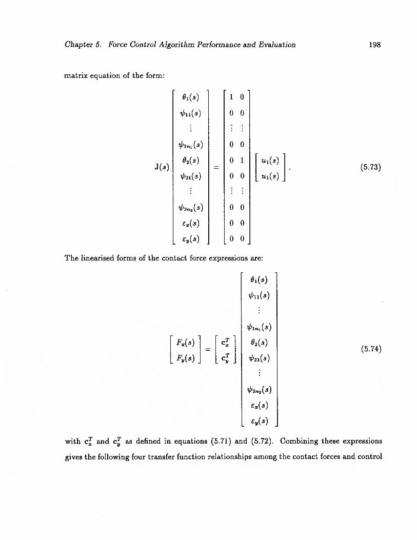
Chapter 5. Force Control Algorithm Performance and Evaluation 198
matrix equation of the form:
8(s) 1 0
0 0
0 0
02(5) 0 1 ui(S)J(s) . (5.73)
b2i(s) 0 0 ui(s)
i1’2n2(8) 0 0
er(s) 0 0
0 0
The linearised forms of the contact force expressions are:
b11(s)
I1ni (s)
Fr(s) c 0(s)
Fr(s) c b2i(s)
i/)2n2(s)
e( s)
with c and as defined in equations (5.71) and (5.72). Combining these expressions
gives the following four transfer function relationships among the contact forces and control

Chapter 5. Force Control Algorithm Performance and Evaluation 199
inputs:rTf \ TrS) CJ1 rS1
— CJ(n1+2)575
ui(s)— J(s)l’ U2(S)
—
and,,j \ T i-i, ‘ Tr,Is) — C ii rs) — Cy J(ni+2)
5 76ui(s) J(3)I’ U2(S) —
where
T / i\(ni+3) 1‘11 i1)
— Ii2I . (_i)’) J(+2)2ii = and J(n+2) =
(—i)(’+”) J1I (_i)(fh+71) J(12)
and J, is the ij minor of the n x n matrix J(s). Note that the transfer functions share a
common denominator, IJ(s). For the case of rigid links the b generalised coordinates are
neglected and the number of admissible functions used to model structural dynamics of the
links, ri1 and n2, are, of course, set to zero.
5.5.3 Force Control for Two Rigid Links
We begin our examination of the performance of the multivariable predictive force control
algorithm with the case of a planar two link manipulator with rigid links. As noted in
section 5.5.1, this case is of theoretical interest in the context of this thesis because it
represents the limiting situation of infinitely link stiffnesses. It is also of practical interest
because most existing industrial manipulators have rigid links.
For this test case the link models are based on the same physical model of a 2.0cm
diameter, 1.Om long aluminium rod that was used throughout section 5.3. The nominal
joint angles are t9 00 and 6 = 300 and the tip of the manipulator is in contact with an
isotropic environment having an effective contact stiffness of keff lOkN/m. The motion
of the manipulator is in the plane perpendicular to the gravitational field.

Chapter 5. Force Control Algorithm Performance and Evaluation 200
Link DynamicsLink (k) 1 26(°) 0 30Lk(m) 1.0 1.0Mk(kg) 0.8451 0.845110k(kg m2) 0.2817 0.2817
Contact DynamicsDirection x yk3(kN/m) 20 20ke(kN/m) 20 20keff(kN/m) 10 10
Table 5.7: Parameter values for two rigid link manipulator controller model.
Controller Model
Using the values listed in Table 5.7 for the parameters of the link and contact dynamics
models the continuous time transfer functions given by equations (5.75) and (5.76) evaluate
to:F’(s) — 1830s2 + 0.4330 x 10⁸
ui(s) — 0.l835s + 77472 + 0.2500 x 10⁸’
Fr(s) — _7464s2— 0.9330 x 10⁸
5 78u2(s) — 0.1835s + 77472 + 0.2500 x 10⁸’
F(s) — _352.1s2 + 0.2500 x 10⁸
ui(s) — 0.1835s + 7747s2 + 0.2500 x 10’
andF(s) — 645152
— 0.2500 x 1085 80
u2(s) — 0.1835s + 7747s2 + 0.2500 x 10⁸
Recalling the results of the linear analysis, for a small contact region mass the dynamics
of the system are dominated by the first two natural modes (see Figure 5.32). For an effective
contact stiffness of keff = 10k N/rn the natural frequencies of those modes are 9.4Hz and
31.3Hz. A sampling frequency of 100Hz (h = lOms) satisfies the Nyquist criterion for those
modes. Assuming zero order hold sampling, the continuous time domain transfer functions

Chapter 5. Force Control Algorithm Performance and Evaluation 201
can be transformed to the following discrete time controller model:
F(q1) — 0.4298 + 0.3909(q1 + q2) + 0.4298q3 1 5 81ui(q1) — 1 — 0.8861q’ + 0.7200q — 0.8861q3+
q_4 ‘
F(q1) — —1.589 — 0.1793(q1+ q2) — 1.589q3 1 5 82u2(q1) — 1 — O.8861q’ + 0.7200q2— 0.8861q3+
q_4 ‘
_______
— —1.698 x 10—2 + 0.4908(q’ + q2) — 1.698 x 10²q35 83
ui(q’) — 1 — 0.8861q’ + 0.7200q2— O.886lq3+ q4q
andF(q1) — 1.165 — 1.639(q1 + q2) + 1.165q3 —‘ 5 84u2(q’) — 1 — 0.886lq’ + O.7200q2— 0.886lq3+
q_4
These polynomials provide the initial model coefficient values for the multivariable adaptive
predictive force control algorithm. They are updated at each time step by a multivariable
form of the EFRA system identification algorithm. The coefficients are also used in con
junction with the closed loop characteristic polynomial formulation derived in section 3.3.1
to tune the control algorithm and analyse its performance by calculating the approximate
closed loop characteristics.
Step Response
The linear analysis in section 5.5.1 suggests that force control for a structurally rigid two
link manipulator using the multivariable predictive control algorithm should be easily ac
complished using a sampling interval sufficient to resolve the 72 mode and a control horizon
of N = 2 time steps. The results presented in this section confirm this prediction.
The approximate closed loop characteristics calculated from the closed loop character
istic polynomial formulation derived in section 3.3.1 show that virtually any combination
of prediction and control horizon values yield stable closed loop performance. However, as
the data in Table 5.8 indicate, a control horizon of N = 2 time steps provides the best
combination of fast rise time and minimal overshoot because the closed loop response is

Chapter 5. Force Control Algorithm Performance and Evaluation 202
Overdamped Mode Underdamped ModesN2 N Dominant Pole fd [Hz] c fd [Hz]3 1 — 7.40 0.678 33.29 0.0885 1 — 7.20 0.389 32.37 0.0428 1 — 7.23 0.090 32.04 0.041
10 1 — 7.35 0.069 32.00 0.035T 2 -134.7 35.14 0.095 — —
5 2 -88.30 35.35 0.077 — —
6 2 -60.37 35.06 0.075 — —
8 2 -26.93 34.32 0.077 — —
10 2 - 9.43 33.91 0.077 — —
5 3 — 40.68 0.032 50.00 0.2348 3 — 39.76 0.002 50.00 0.4735 4 — 39.96 0.019 50.00 0.0928 4 — 39.77 0.005 50.00 0.188
Table 5.8: Stabilising controller horizons and closed loop characteristics for a structurallyrigid two link manipulator contacting a keff = kN/m surface. Id = damped natural frequency and damping ratio.
composed of one overdamped and one underdamped mode. For all other control horizon
values both of the closed ioop modes are underdamped. Figure 5.40 shows the contact force
step responses in the world frame x and y directions and the control inputs (joint torques)
for the case of a 2 time step control horizon and a prediction horizon of N2 5. As can
be seen, this combination of controller horizons yields a fast, offset free step response with
negligible overshoot. Reducing the prediction horizon to N2 = 4 moves the dominant pole
of the overdamped mode farther to the left on the real axis, thereby producing a somewhat
faster rise time but this is accompanied by a slight overshoot due to the 35Hz mode. On
the other hand, increasing the prediction horizon only results in slower rise times.
5.5.4 Force Control for Two Flexible Links
To demonstrate the performance of the multivariable predictive control algorithm for the
case of flexible links we will examine the case of a two link manipulator with identical links

Chapter 5. Force Control Algorithm Performance and Evaluation 203
(a) direction contact force (b) y direction contact force
14
13
12
11
10
E9z
01.—aC05-
4
3
2
0 .05 .10 .15 .20 .25 .30 .35 .40
Time [s]
(c) Joint torques
Figure 5.40: Force control step responses for a structurally rigid two link manipulatorcontacting a keff = lOkN/m surface with N2 = 5, N = 2, ) = 0.
11
10
9
8
C04
C)
3
2— Response
Setpoint
11
10
9
8
7
6
5
4
3
2
ci)C)0
cicciC00
0 .05 .10 .15 .20 .25 .30 .35 .40 “0 .05 .0 .15 .20 .25 .30 .35 .40Time [s] Time [SI
— ResponseSetpoint
— Joint 1Joint 2

Chapter 5. Force Control Algorithm Performance and Evaluation
in which the link structural dynamics are modelled by one admissible function per link.
The link models are based on the same physical model of a 2.0cm diameter, l.Om long
aluminium rod that was used throughout section 5.3. The nominal joint angles are 19 = 00
and 6 = 30° and the tip of the manipulator is in contact with an environment having an
isotropic environment with a effective contact stiffness of keff = lOkN/m. The motion of
the manipulator is in the plane perpendicular to the gravitational field.
Controller Model
Table 5.9 lists the numerical values of the link and contact dynamics model parameter for
the system. Using these values the transfer functions given by equations (5.75) and (5.76)
evaluate to:
Fr(s) —36.49s6 — 1.56 x 10⁶s4 + 1.95 x 10h1s2 + 2.18 x iO’ui(s)
— IJ(s)I
Link Dynamics
204
Link (k) 1 28(°) 0 30Lk(m) 1.0 1.0Mk(kg) 0.8451 0.84517J0k(kg.m2) 0.2817 0.2817Tlkl(kg m2) 0.4807 0.480712k1(kg.m2) 0.8451 0.845113k1(N m) 7096 7096I4k(kg.m) 0.6617 0.6617cIk1o(m) 2.0 2.0ç1410(m/m) 2.753 2.753
Contact DynamicsDirection x yk(kN/m) 20 20ke(kN/m) 20 20keff(kN/m) 10 10
Table 5.9: Parameter values for two flexible link manipulator controller model
(5.85)

Chapter 5. Force Control Algorithm Performance and Evaluation 205
Fr(s) —
_289.3s6— 6.67 x — 2.95 x 10’2s2 — 1.18 x 10¹⁶
5 86U2(S)
-
Fr(s) —
_3.26s6 + 3.47 x i0s — 2.96 x 10¹⁰s2 + 1.26 x 1O’5 87
ui(s)-
andF(s) — _29.85s6
— 3.60 x 106.s4 + 2.40 x 10u1s2— 1.26 x 1O’
(5 88)u2(s)
where
= (1.39 x 10⁴s8+ 88.05s6 + 1.36 x 10⁷s4 + 4.08 x 101182 + 1.26 x 10¹⁵). (5.89)
Figure 5.41 shows the natural frequencies of the first four modes of the system as a
function of keff with keff = lOkN/m marked. At this effective contact stiffness the frequencies
of the 7h and 772 modes are in the region of approximate proportionality to kff and therefore
make significant contributions to the dynamics. The mode frequency is independent
of keff and the 774 mode frequency is just entering the transition range. The open ioop
natural frequencies of the modes are 9.39Hz, 29.7Hz, 67.5Hz and 102Hz. Sampling at
250Hz (h = 4ms) to satisfy the Nyquist criterion for the mode results in the following
discrete time transfer function models for the controller:
F —1 — Bi(q1)ui +B2(q1)u2 —i(q
— A —‘ q (.
and
FBi(q)ui +B2(q’)u2 —1
Y A —i q ,
where
A(q’) = 1— 1.48q’+0.67q2—0.34q3+0.54q4—0.34q5+0.67q6—1.48q7+q8,(5.92)
Bi(q’) = —0.81 +3.76q’ —5.20q2+2.46(q3+q4)—5.20q5+3.76q6—0.81q7, (5.93)
B2(q1) —9.47+18.5q’—17.0q2+6.79(q3+q4)—17.0q5+18.5q6—9.47q7,(5.94)

Chapter 5. Force Control Algorithm Performance and Evaluation 206
iø
1OkN/rn.
101
2//
iOø I I iiiil I iiiiiil I hull1 uuuuuul lulihul I 1111111
10_2 i00 101 102 iø
Effective Contact Stiffness [kN/m]
Figure 5.41: Variation of the natural frequencies for a two link manipulator with identicalflexible (El = 574N m2, one structural mode each) links assuming steady state contactdynamics and an isotropic environment.

Chapter 5. Force Control Algorithm Performance and Evaluation 207
—0.047q’ — 0.87q2 + 0.70(q3+ q4) — 0.87q5+ 0.34q6— 0.047q7, (5.95)
and
B2(q’) = —0.78+2.91q’ —2.61q2+0.36(q3+q4)—2.61q5+2.91q6—0.78q7. (5.96)
These polynomials provide the initial model coefficient values for the multivariable adaptive
predictive force control algorithm. They are updated at each time step by a multivariable
form of the EFRA system identification algorithm. The coefficients are also used as part of
the technique developed in section 3.3.1 to analyse the performance of the control algorithm
by calculating the approximate closed loop characteristics.
Step Response
The results plots presented in the first part of this section are from a simulation using
the linearised manipulator dynamics. This is done in order to minimise the mismatch be
tween the controller model and the system dynamics so that attention can be focussed on
the performance of the control algorithm. Later in the section results from the nonlinear
dynamics simulation are shown. These results demonstrate the role that the system identi
fication algorithm plays in the adaptive controller, namely, compensating for the presence
of unmodelled, nonlinear components of the manipulator dynamics.
Examination of the approximate closed loop poles, calculated from the control law and
the linearised system dynamics, shows that with N = 1 all prediction horizons which give
stable control result in all of the closed loop modes being underdamped. The resulting
response therefore exhibits undesirable overshoot and oscillations about the setpoints. This
poor control is not surprising in light of the fact that there are two dominant modes in
the system. Allowing the controller only one time step in which to minimise the predicted
error does not provide enough freedom to deal with two modes. Better control is obtained
with N = 2, that is, the control horizon equal to the number of dominant open loop

Chapter 5. Force Control Algorithm Performance and Evaluation 208
Overdamped Mode Underdamped ModesN2 iç Dominant Pole Id [Hz] C fd [Hz] C fd [Hz] C9 2 -91.87 23.20 0.675 32.74 0.222 101.2 0.05515 2 -103.6 12.43 0.889 36.51 0.174 98.99 0.05218 2 -39.86 30.91 0.447 35.51 0.297 100.1 0.06020 2 -25.58 31.96 0.187 39.02 0.423 99.63 0.04422 2 -17.55 30.89 0.165 44.43 0.351 99.44 0.0486 3 -41.98 37.15 0.040 89.77 0.045 125.0 0.290
25 3 -49.95 35.63 0.008 99.62 0.002 125.0 0.8478 4 -92.27 35.16 0.010 96.12 0.012 125.0 0.34210 4 -78.50 35.57 0.029 95.24 0.014 125.0 0.39112 4 -65.09 35.78 0.016 96.50 0.010 125.0 0.466
Table 5.10: Stabilising controller horizons and closed ioop characteristics for a two flexiblelink (one structural mode each) manipulator contacting a keff = lOkN/m surface. Id =damped natural frequency and C = damping ratio.
modes. The closed ioop response is composed of one overdamped and three underdamped
modes. The top part of Table 5.10 shows the approximate continuous time closed ioop
characteristics for various values of N2. In this case the closed loop performance is largely
governed by the time constant of the overdamped mode and the damping ratio of the
lowest frequency underdamped mode. With a 2 step control horizon, N2 = 20 provides the
response with the fastest rise time and no overshoot, as can be seen in Figures 5.42a and
5.42b. A shorter prediction horizon causes the rise time to be such that the oscillations of
the underdamped modes do not completely damp out before the setpoint is reached and
the response overshoots. Longer prediction horizons result in unnecessarily slow responses.
With a control horizon of 3 time steps the closed system generally has four under
damped modes, but for selected prediction horizons (see Table 5.10) the response has one
overdamped mode and three underdamped ones. In the case of four underdamped modes
one of the modes is always of very low frequency and has a relatively high damping ratio.
While the step response with these characteristics will, by definition, always exhibit over
shoot, if the damping ratio of the lowest frequency mode is sufficiently high the overshoot

Chapter 5. Force Control Algorithm Performance and Evaluation
12
F:
2
30
28
26
24
22
18a)D 160
14
12
-, 10
8
6
4
2
0
(a) a direction contact force
(c) Joint torques
(b) y direction contact force
(d) Link tip deflections
Figure 5.42: Force control step responses for linear dynamics simulation of a two flexible link(one structural mode each) manipulator contacting a keff = l0kN/m surface with N2 = 20,N = 2, 0.
14
209
F’a)C-)
0U
C0
C-)
0
— ResponseSetpoint
.05 .10 .15 .20 .25 .30 .35 .40 .45 .50 .55 .60
Time [s]
ResponseSetpoint
0 .05 .10 .15 .20 .25 .30 .35 .40 .45 .50 .55 .60
Time [s]
.05 .10 .15 .20 .25 .30 .35 .40 .45 .50 .55 .60
Time tsl

Chapter 5. Force Control Algorithm Performance and Evaluation 210
will be negligible. As noted in section 5.3.5 the possibility of one of the closed ioop modes
changing from being overdamped to being underdamped may be cause for concern regarding
the robustness of the control law.
With N = 4 the controller has a control horizon equal to the total number of modes
in the open loop system. Table 5.10 indicates that the lowest frequency closed ioop mode
which dominates the response when N = 2 has been completely removed and a light
damped 125Hz mode (half the sampling frequency) has appeared. The dominant pole of
the overdamped mode is generally more negative than is the case with Nu < 4, indicating
that the rise time is decreased. Figure 5.43 shows the step responses for the case of N2 = 8
and N = 4. The faster response of the N 4 controller compared to the N = 2 is
the result of a much more active control input signal as can be seen by comparing Figures
5.42c and 5.43c. Increasing the prediction horizon from 8 time steps generally increases the
damping of the closed ioop modes, thereby reducing the ripple in the response but only at
the expense of increased rise times.
The step responses examined so far have concentrated on the case of simultaneous
changes in the x and y direction contact force setpoints. Another important aspect of the
closed ioop performance, given the strongly coupled nature of the system, is the interaction
of the outputs. This aspect is illustrated by commanding a step change in one output while
holding the other setpoint constant. Figure 5.44 shows the responses under these conditions
that results from controller horizons of N2 = 20 and N = 2 and Figure 5.45 shows the
corresponding results with N2 = 8 and N = 4. These figures show that the disturbance
of one component of the contact force which occurs in response to a step change in the
setpoint of the other component is of much larger magnitude and longer duration when the
N = 2 controller is used rather than N = 4. The difference in duration of the disturbance
is due in part to the anticipation characteristic of predictive control and results from the
difference in prediction horizons. The difference in magnitude is due to the difference in

Chapter 5. Force Control Algorithm Performance and Evaluation
zci)C)0
LL
C)CuC0
C.)
32
30
28
26
24
18D216
1214
C0
—, 10
8
6
4
2
0
(a) direction contact force
(c) Joint torques
(b) y direction contact force
(d) Link tip deflections
Figure 5.43: Force control step responses for linear dynamics simulation of a two flexible link(one structural mode each) manipulator contacting a keff = lOkN/m surface with N2 = 8,N = 4, ) = 0.
211
16
14
12
10
8
6
4
2— Response
Setpoint
ci)C)0
C)(8C00
IL
.05 .10 .15 .20 .25 .30 .35 .40 .45 .50 .55.
Time [s]
— ResponseSetpoint
35 .40 .45 .50 .55
Time [s]
0 .05 .10 .15 .20 .25 .30 .35 .40 .45 .50 .55 .60
Time [s] Time [s]

Chapter 5. Force Control Algorithm Performance and Evaluation
2’
C)0U
C0
C.)
212
Figure 5.44: Force control step responses showing output interactions for linear dynamics simulation of a two flexible link (one structural mode each) manipulator contacting akeff = lOkN/m surface with N2 = 20, N 2, 0.
16
14
12
10
8
6
4
2
0
ResponseSetpoint
ci)C)0
LlC)cciC0
C.)
II
.1 .2 .3 .4 .5
Time [s].6 .7 .8 .9 1.0
(a) direction contact force
0 .1 .2 .3
— Response- Setpoint
.4 .5 .6 .7 .8 .9 1.0
Time [s]
(b) y direction contact force
34
32
30
28
26
24
E 22
-201)D 180
16
14CO 12-3
10
a6
4
2
0
Time [s] Time [s]
(c) Joint torques (d) Link tip deflections

Chapter 5. Force Control Algorithm Performance and Evaluation
20
18
16
14G)o 0
12LI
10
Eo 0o 0
6
4
2
25
200
0-)
Figure 5.45: Force control step responses showing output interactions for linear dynamics simulation of a two flexible link (one structural mode each) manipulator contacting akeff = lOkN/m surface with N2 = 8, N 4, 0.
213
16
14
12
10
8
6
4
2
0
Response-. Setpoint
1’
I .1 .2 .3 .4 .5 .6 .7 .8 .9 1.0
Time [s]
(a) direction contact force
— Response- Setpoint
40
35
.1 .2 .3 .4 .5 .6 .7 .8 .9 1.0
Time [s]
(b) y direction contact force
30
10
5
.1 .2 .3 .4 .5 .6
Time [s]
(c) Joint torques
.1 .2 .3 .4 .5 .6 .7 .8 .9 1.0Time [s]
(d) Link tip deflections

Chapter 5. Force Control Algorithm Performance and Evaluation 214
the lowest closed ioop natural frequencies and the degree to which they are excited. The
disturbance of the y direction contact force due to a step change in the x direction is less
significant than when the situation is reversed but the trends of magnitude and duration of
the disturbance are comparable. The generally better performance in the y direction shown
in all of the above figures is due primarily to the 8 0°, 0 30° configuration of the
manipulator.
All of the preceding simulation results in this section are based on a simulation of the
linearised equations of motion. Under those circumstances the controller model and the
system dynamics are exactly matched. When the full, nonlinear dynamics of the system
are considered the situation is somewhat more complicated. The nonlinearities represent,
from the point of view of the controller, unmodelled dynamics. The controller is able to
cope with the unmodelled dynamics due to its explicitly adaptive implementation, that
is, at every time step the system identification algorithm calculates a new estimate of the
coefficients of the controller model. These coefficients are presumed to accurately represent
the instantaneous system dynamics in a linear form and are used to calculate the control
input for the next time step. Figure 5.46 shows a series of step responses from the nonlinear
dynamics simulation for the same manipulator and environment configuration used above.
The controller has a prediction horizon of N2 = 20 time steps and a control horizon of N = 2
steps. During the early part of the response the mismatch between the controller and system
dynamics results in strong excitation of the high frequency modes. The high frequency
structural vibrations of the links are evident in the plot of the local defiections of the link
tips shown in Figure 5.46d. These vibrations are also evident in the plots of the contact force
components (Figures 5.46a and 5.46b). In order to control the high frequency modes the
control inputs are forced to switch rapidly over relatively large amplitudes (Figure 5.46c).
While this high frequency activity results in a relatively poor response with a great deal of
overshoot it also provides rich excitation for the system identification algorithm with the

Chapter 5. Force Control Algorithm Performance and Evaluation
a) Q)o 0o o
U
(aC Co 0o C)
Figure 5.46: Force control step responses for nonlinear dynamics simulation of a two flexiblelink (one structural mode each) manipulator contacting a keff = lOkN/m surface withN2=2O,N=2,)=O.
215
11
— ResponseSetpoint
20
18
16
14
12
10
8
6
4
2
0
45
40
35
0 .2 .4 .6 .8 1.0 1.2 1.4 1,6 1.8
Time [SI
(a) a direction contact force
0 .2 .4 .6
— ResponseSetpoint
.8 1.0 1.2 1.4 1.6 1.8
Time Is]
(b) y direction contact force
3Ø
za) 250’
1S 20
0—, 15
10
Time [s]
(c) Joint torques (d) Link tip deflections

Chapter 5. Force Control Algorithm Performance and Evaluation 216
result that after 0.8s (200 time steps) the controller model coefficients have been sufficiently
well adjusted to compensate for the unmodelled nonlinear dynamics and the subsequent step
responses are much improved.
It is not surprising that the effect of the unmodelled nonlinear dynamics is much more
pronounced in the case of the two link manipulator than was observed in the single link
results when the structure of the equations of motion for the two cases are compared. The
number of centripetal and Coriolis terms in the two link equations of motion far exceeds
those in the single link equations. In particular the two link equations have a large number of
terms which represent interactions between the joint angle and modal amplifier generalised
coordinates both for a given link and between one link and the other.
The results shown in Figure 5.46 demonstrate the limitations of the application of a
strictly linear controller to a highly nonlinear system. Several possibilities for improvement
of the closed loop performance can be considered. The simplest is filtering of the high fre
quency component of the response which would reduce the amplitude of the disturbances
but would likely also increase the time required for the identification algorithm to arrive
at a suitable model. A more fruitful approach might be to model the disturbances due to
the nonlinear unmodelled dynamics as coloured noise and include the noise model in the
controller model [32]. In either case the effect of the nonlinear dynamics can be substan
tially reduced by specifying setpoint programs which would produce less excitation of the
structural dynamics modes that the step changes shown in Figure 5.46. Ramps or higher
order polynomials would provide smoother transitions between setpoint levels and therefore
reduce the level of excitation. Reformulation of the predictive control algorithm on the
basis of a nonlinear model (for example [90]) could also be considered.

Chapter 5. Force Control Algorithm Performance and Evaluation 217
5.5.5 Summary
In summary, this section has presented an analysis of force controlled two link manipulators
with rigid or flexible and an evaluation of the performance of the multivariable, adaptive,
predictive control algorithm applied to the control of world frame contact force components
exerted by the manipulator tip on environment surfaces.
Linear analysis of the case of infinitely stiff links reveal the expected extension of char
acteristics which were identified in the single link case while at the same time illustrating
the added complexities of the two link system. The modal frequencies are found to vary
with k!ff for a given set of link lengths and inertias and the two highest frequency modes
are due to the local vibrations of the contact region mass. The frequencies are independent
of when the contact is isotropic (kxeff = kyeff) and are bounded above by the values for
é1 = 900. The contributions of the natural modes to the contact force components are also
found to vary with the nominal manipulator geometry. With the addition of modes due to
the structural flexibility of the links, linear analysis reveals a transfer of dominance among
the modes similar to that seen in the single link case, but with the expected additional
dependence on joint angles.
A transfer function model of the system which relates the world frame x and y direction
components of the contact force to the joint inputs was derived on the basis of the linearised
equations of motion. Specific parameter values were selected for a manipulator with two
identical links in contact with a relatively stiff (keff = lOkN/m) isotropic (k =k) environ
ment. The links were based on the physical model of 1.Om long, 2.0cm diameter aluminium
rods. Cases in which the link are assumed rigid as well as having their structural dynamic
modelled using the first mode shape function of the rods considered as a cantilever beams
have been addressed.

Chapter 5. Force Control Algorithm Performance and Evaluation 218
As in the single link case, the approximate closed ioop characteristics calculated from the
control law were found to be very useful in selecting controller horizons which produced the
fastest rise times and least overshoots from among the large set of horizons which stabilise
the system.
5.6 Force Control for DC Motor Actuated Space Station Manipulator
As a final demonstration of the performance of the multivariable predictive force control
algorithm we will examine the case of a simple prototype model of the two long links of the
proposed Mobile Servicing System (MSS) for the Space Station Freedom. These massive,
long, slender links are driven by geared direct current motors at their joints. The physical
parameter values for the system are listed in Table 5.11. The top part of the table shows
the link model parameter values which are based largely on those used by Chan [68]. The
MSS manipulator operates in a microgravity environment in which the gravitational field
is approximately balanced by the orbital centripetal acceleration and thus the gravitational
loading of the links is neglected in the model. The center section of the table shows the
parameters used to model the DC motors. Since the motor parameters are not publically
available the values shown are estimates based on assumptions of a maximum motor power
of 400W and a maximum torque delivery of 1500N m. Due to the mass of the links, the
natural frequencies of the cantilever beam modes used as admissible functions to model the
link structural dynamics are much lower than in the previously considered cases. In fact
the frequency of the first mode is only about 0.3Hz. Even when the tip of the second link
is in contact with a surface with very high effective contact stiffness the natural frequencies
are all less than 30Hz (see Figure 5.47).
The controller model structure is similar to that derived in section 5.5.2. The control
inputs are the input voltages to the motors. These voltages are amplified to produce the

Chapter 5. Force Control Algorithm Performance and Evaluation 219
Link DynamicsLink (k) 1 2
(°) 0 30Lk(m) 7.5 7.5Mk(kg) 1600 1600IOk(kg m2) 3.0 x i0 3.0 x iOIlkl(kg . m) 6826 682612k1(kg.m) 1600 160013k1(N.m) 6388 6388141C1(kg.m) 1253 12534k1o(m) 2.0 2.0qYklO(m/m) 0.3671 0.3671
Actuator DynamicsJoint (k) 1 2Iak(kg m2) 0.5 0.5Ngk () 50. 50.Rak(Q) 1.0 1.0Kk(N . rn/A) 1.5 1.5Kem(V s/rad) 0.5 0.5K(V/V) 4.0 4.02akmax(A) 20. 20.Vznkmax(V) 5.0 5.0
Contact DynamicsDirection x yk(kN/m) 40 40ke(kN/m) 40 40keff(kN/m) 20 20
Table 5.11: Physical parameter values for a two link MSS model with DC motor actuators.

Chapter 5. Force Control Algorithm Performance and Evaluation 220
210 I I 1111111 I I 1111111 I 11111111 11111111 I I 1111111
101
1 0
D- I
z I
10-
I
11,
1_2 i ii I I I ii I I I I I ii I I I I II I
10_i 1& 102 iø
Effective Contact Stiffness [kN/m]
Figure 5.47: Variation of the modal natural frequencies for DC motor actuated two linkMSS model.

Chapter 5. Force Control Algorithm Performance and Evaluation 221
armature circuit voltages which in turn produce the armature currents to which the torques
supplied by the motors are proportional. Thus, the discrete time transfer function models
for the controller are of the form:
—1 Bi(q1)vi +B2(q1)v2 _.iF(q ) = A(q1)q (5.97)
and
F— Bi(q1)vi +B2(q’)v2 —1 5 98Y— A(q1)
q
With the manipulator in contact with a surface such that the effective contact stiffness is
2OkN/m, the open loop natural frequencies of the first four modes of the system are 0.30Hz,
0.90Hz, 1.5Hz and 2.4Hz. As can be seen in Figure 5.47, the mode is, at keff = 2OkN/m,
in transition between being independent of lCeff and being proportional to kff and therefore
contributes significantly to the contact force. To satisfy the Nyquist criterion for the
mode a sampling frequency of 7.7Hz (h = l3ms) is used.
Figure 5.48 shows the contact force responses from the linearised dynamics model of the
MSS controlled by the adaptive, multivariable predictive control algorithm with N2 = 14,
N = 2, k = 0 and .Xse = 0. Note that the time scale of the figures in this section is much
longer than that of the previously shown results owing to the much greater mass of the
MSS links compared to aluminium rod links used in the previous cases. The y direction
contact force setpoint in Figure 5.48 consists of a smooth transition between force levels.
The transition is constructed by matching exponential functions of the form et— 1 and
1 —
et at the midpoint of the transition. The direction goal is to maintain a constant
force level. Figure 5.49 shows the responses of the full nonlinear dynamics model with
the same setpoints and controller parameters. These results illustrate the improved per
formance for the nonlinear case (compared to Figure 5.46) which is obtained by using a
smooth setpoint transition as opposed to a step change. The relatively small magnitude of
the level change also contributes to the improved performance. Both of these factors result

Chapter 5. Force Control Algorithm Performance and Evaluation
5.5
5.0
4.5
4.0
a)0
C00
3.0
2.5
2.0
1.5
1 .0
.5
0>
0.
z
0U
0(aC00
EEC0C)
a)
0.I
C-J
222
Figure 5.48: Force control responses for linear dynamics simulation of a two flexible linkSpace Station MSS contacting a keff = 2OkN/m surface.
.4.5
4.0
/7I1/
3.0
2.5
2.0
1.5
1 .0
— Response.5 .
..---. Setpoint
0.1,1 1,1. .1, I. .1.1.1.
0 2 4 6 8 10 12 14 16 18 20 22 24 26 28 30Time [s]
(b) y direction contact force
r— Response
2 4 6 8 10 12 14 16 18 20 22 24 26 28 30Time [s]
(a) n direction contact force
- 060 2 4 6 8 10 12 14 16 18 20 22 24 26 28 30
Time [s]
(c) Motor input voltages
2 4 6 8 10 12 14 16 18 20 22 24 26 28 30
Time [s]
(d) Link tip deflections

Chapter 5. Force Control Algorithm Performance and Evaluation
5.5
5.0
4.5
3.50
Li_
C)a)C0
C.)
2.5
2.0
1.5
1.0
.5
.35
.30
.25
.20
.15(a
.10>
.05
C— 0
-. 05
- .10
- .15
-. 20
223
(c) Motor input voltages (d) Link tip deflections
Figure 5.49: Force control responses for nonlinear dynamics simulation of a two flexible linkSpace Station MSS contacting a keff = 2OkN/m surface.
5.0
4.5
4.0
3.5
3.0
2.5
2.0
a)0
0U
00
.
... .
— Response r— Response----- Setpoint .5
. L- Setpoint
.1 .1. .1.1.. .1.1.1. 0 .1. .1.1. .1.1.
0 2 4 6 8 10 12 14 16 18 20 22 24 28 28 30 0 2 4 6 8 10 12 14 16 18 20 22 24 26 28 30Time [s] Time [s]
( a) z direction contact force (b) y direction contact force
4 • 1.5
— Joint 1 1 I 1 .0 — — —... link 1
--- Joint 2 ii L- -
- link 2
aE. -.5C.2 -1.0
.,j I’.. —.
0 2 4 6 8 10121416182022242628
Time [s]30 14 16 18 20 22 24 26 28 30
Time [s]

Chapter 5. Force Control Algorithm Performance and Evaluation 224
in less excitation of the nonlinear dynamics of the system which are not included in the con
troller model. While the improvement in the system performance is encouraging, additional
filtering and/or reformulation of the control algorithm, as discussed in section 5.5.4, would
be necessary to meet the expected operational performance specifications for the MSS.
5.7 Summary of Force Control Performance
The simulation results in this chapter have demonstrated the viability of the use of a
multivariable, explicitly adaptive, long range predictive control algorithm to control the
contact forces exerted by manipulators on surfaces in their working environment. The
following configurations were considered:
• a single flexible link with its structural dynamics modelled by one, two and three ad
missible mode shape function in contact with surfaces with effective contact stiffnesses
ranging from 3.1kN/n to 5MN/m;
• the same link, initially under motion control, making unexpected contact at an impact
velocity of approximately O.5m/s with a surface;
• a planar, two link manipulator with rigid links in contact with an isotropic effective
contact stiffness of lOkN/m;
• the same two link manipulator with the structural flexibility of the link modelled by
one admissible mode shape function for each link, also making contact with a surface
such that the isotropic effective contact stiffness is keff = lOkN/m; and;
• a prototype model of the two long links of the DC motor actuated Mobile Servicing
System (MSS) manipulator for the proposed Freedom Space Station, with its tip in
contact with a keff = 2OkN/m surface.

Chapter 5. Force Control Algorithm Performance and Evaluation 225
The single flexible link step response results demonstrate that with a controller model of
appropriate order and a sampling rate selected to resolve the dominant mode, as indicated
by the shape of a frequency versus effective contact stiffness plot, there are generally a wide
range of control algorithm horizon and weighting factor values for which the closed ioop
will be stable. The inherent integral action of the control algorithm guarantees that the
response will not have a steady-state offset. A new formulation for the discrete time domain
closed ioop characteristic polynomial has been used to select control algorithm horizons and
weighting factors to satisfy additional performance requirements such as minimal overshoot
and rise time. The inclusion of a static equilibrium bias term in the controller has been
shown to decrease rise time at the expense of introducing a slight amount of overshoot into
the response. The importance of selecting a reasonably accurate initial controller model
implies that knowledge of the structural dynamics of the manipulator and the contact
characteristics of the surfaces likely to be encountered in the workspace is necessary to
ensure successful control.
The problem of maintaining control while unexpectedly making contact with a surface
is a challenging one because the complex dynamics of the system are compounded by the
presence of a discontinuity. To cope with this problem a contact control logic level has
been introduced into the manipulator control hierarchy. Two operational strategies for the
contact control logic have been demonstrated and shown to allow control to be maintained
through contact events, albeit with some unavoidable contact force transients. Of par
ticular interest is the fact that under the setpoint modification strategy there is a direct
relationship between the impact velocity and the magnitude of the initial force transient.
This relationship allows manipulator motions, in particular tip velocities, to be planned on
the basis of the transient contact force levels to which nearby surfaces can be acceptably
subjected, should a collision occur.

Chapter 5. Force Control Algorithm Performance and Evaluation 226
The step response results for the case of a two link manipulator with a rigid structure
show that the controller has the potential to provide excellent force control performance for
this large subset of existing industrial manipulators. In this context, the predictive control
algorithm could be readily incorporated into a combined force and motion control structure,
such as the hybrid methodology of Raibert and Craig [12]. This case is also of interest as
the limiting situation of infinite structural stiffness because it offers validation of some of
the fundamental conclusions of the linear analysis developed in this chapter.
With the inclusion of structural flexibility the dynamics of the two link manipulator
become markedly more complex and nonlinear. The results demonstrate that the insight
gained from the linear analysis of the system and the calculation of the roots of the close
loop characteristic polynomial offer guidance in this case, as in the less complex cases, in
the construction of the controller model and the selection of control algorithm horizons and
weighting factors to provide the most desirable response. The simulations also show that
the strongly coupled structure of the manipulator dynamics, combined with the optimal (in
the sense of minimising a cost function based on predicted output errors) form of the control
law, make total isolation of the controlled quantities impossible. That is, the response to a
step change commanded for one component of contact force will result in some disturbance
of the other component.
The highly nonlinear nature of the two flexible link manipulator dynamics presents some
difficulty for the inherently linear control algorithm. The unmodelled, nonlinear dynamics
are compensated for, to some extent, by the adaptive structure of the controller but it has
been found that it is possible to excite the unmodelled dynamics to such an extent that
stability is lost. Several potential remedies to this problem are possible including filtering of
the contact force signals, using smooth setpoint transitions instead of steps, inclusion of a
coloured noise model in the control algorithm formulation, and rederivation of the predictive
control algorithm on the basis of a nonlinear model.

Chapter 5. Force Control Algorithm Performance and Evaluation 227
rpIle force control simulations for the Space Station Mobile Servicing System (MSS) ma
nipulator model demonstrate the effectiveness of the controller with a manipulator having
radically different dynamic parameters from those considered previously. The model in
cludes voltage controlled DC electric motor actuators which drive the joints through gear
boxes. The force control results show that the use of smooth setpoint transitions attenuates,
to some extent, the difficulties caused by unmodelled, nonlinear dynamics.
Chapter 6
Summary of Major Results
This thesis has developed and demonstrated an overall strategy for the control of contact
forces exerted by a structurally flexible manipulator on surfaces in its working environ
ment. The control strategy is centered on an explicitly adaptive implementation of a pre
dictive control algorithm based on the Generalised Predictive Control algorithm of Clarke,
et al. [29]. The thesis also presents analyses of the linearised equations governing the manip
ulator/environment system in several configurations, using a combination of analytic and
numerical techniques. The results of these analyses provide insight into the fundamental
dynamics which dominate the force controlled system. These insights are used to guide the
selection of the appropriate controller model and parameters for particular configurations.
The major contributions of the research reported in this thesis are:
• Kinematic and dynamic models of flexible link manipulator interacting with surfaces
in its working environment has been developed. The model includes the effects of
local inertia, energy dissipation and surface stiffnesses of the contacting surfaces of
the manipulator tip and the environment. Analysis shows that when the mass of the
surface regions deflected due to contact is comparable to the inertias of the links the
inertia effects in the contact model become important.
• Linear analyses of various configurations of manipulators in contact with environment
surfaces have been carried out using a combination of analytic and numerical tech
niques. The results of these analyses provide new insights, not apparently available
228

Chapter 6. Summary of Major Results 229
in the literature, into the fundamental dynamics of the system using established lin
ear analysis methods. In particular, they reveal that the contact force response is
dominated by different open loop modes, depending on the effective stiffness of the
contacting surfaces and that the transfer of dominance among the modes follows an
orderly progression from lower to higher frequency modes as the effective contact stiff
ness is increased in a given configuration. The analyses also show that the control
inputs tend to provide excitation to all but the very high frequency contact vibration
modes. The implications of these two results for the design of discrete time domain
contact force controllers are that the loop must be closed at a sampling frequency suf
ficient to resolve the dominant mode in the contact force response and the controller
model must include the dynamics of all of the excited modes. The linear analyses
provide guidance in determination of the dominant and significantly excited modes
for a particular manipulator configuration.
• A new general formulation for the closed loop characteristic polynomial of a system
controlled by the Ceneralised Predictive Control (GPC) algorithm has been obtained
in the discrete time domain. The formulation is applicable to both the original single
input, single output form of the algorithm and to its multivariable extension. Cal
culation of the approximate closed loop characteristics of the system from this result
has been shown to be useful in tuning the control law for particular configurations.
• The predictive control algorithm has been extended with a static equilibrium bias
term in the cost function. This extension is applicable to both SISO and multivariable
forms of the algorithm. The addition of this new term augments the feedback control
law with a proportional action feedforward component. The static equilibrium bias
term is particularly applicable in the contact force control application because of the

Chapter 6. Summary of Major Results 230
easily defined static equilibrium relationship between joint torques and contact force
components.
• Contact control logic is introduced as a first step in the integration of the predictive
control algorithm into an overall force/motion control strategy. In the form presented,
the primary function of the contact control logic is to deal with the discontinuity
involved in making and breaking contact and collisions between the manipulator tip
and the environment surface due to unexpected contact events.
• Detailed simulation results for one and two flexible link manipulators have been pre
sented. The results demonstrate that the predictive control algorithm can be tuned
to provide fast step responses with minimal overshoot for a wide variety of manipu
lator configurations and contact stiffnesses. The importance of the effective contact
stiffness in the dynamic structure of the system indicates the need for some a priori
knowledge of the surfaces a given manipulator is likely to contact during particular
operations.
• Two operational strategies for the contact control logic have been demonstrated in
the situation of a collision due to an unexpected contact event. The setpoint modifi
cation strategy was found to be superior to the stop motion strategy, which tends to
induce bouncing on the surface. In the setpoint modification strategy joint and force
sensor data around the instant of contact are used to predict the characteristics of
the expected force transient and the contact force setpoint is then briefly increased to
allow the controller to supply more energy to overcome the unexpected force transient
due to the kinetic energy transferred from the link to the surface.
• The explicitly adaptive implementation of the predictive force control algorithm using
the Exponential Forgetting and Resetting Algorithm (EFRA) for system identification

Chapter 6. Summary of Major Results 231
has been found well capable of compensating for unmodelled structural modes in the
single link case. The unmodelled nonlinear dynamics in the two link case present a
greater difficulty which significantly limits the performance of the controller.
6.1 Recommendations for Further Research
The following directions for future research stemming from the results of this thesis are
recommended:
• integration of the predictive control algorithm for force and motion control of flexible
link manipulators into the framework for simultaneous force and motion control such
as the hybrid position/force control framework of Raibert and Craig [12];
• extension of the contact control logic concept to deal with a wider range of making
and breaking contact events; this may be a suitable application for fuzzy control;
• improvement of the force control algorithm in situations where significant unmodelled
nonlinear dynamics exist; possible actions are simple filtering, inclusion of a coloured
noise model in the controller model, selection of setpoint programs less likely to excite
the nonlinear dynamics, and reformulation of the predictive controller on the bassis
of a nonlinear model.
Implementation Issues
Early in the course of the research force control experiments were conducted in which a
version of the damping algorithm introduced by Whitney [3] was implemented on a Puma
560 robot equipped with a JR3 force sensor. Edge following and peg—in—hole operations were
successfully demonstrated. Unfortunately, the closed architecture of the Puma controller,
its relatively slow ioop closing time (‘-. 28ms), and the unsuitability of the interpreted Val

Chapter 6. Summary of Major Results 232
II controller programming language for extensive mathematical computations precluded
the implementation of a more complex predictive force control algorithm.
The experiments with the Puma 560 robot and the JR3 force sensor demonstrated
two characteristics of the force sensor which can pose difficulties. Firstly, under some
circumstances the raw sensor signal was found to be quite noisy. The JR3 sensor firmware
includes digital filtering capabilities which allowed a much cleaner signal to be obtained
without appreciable loss of accuracy for the operations undertaken. The second problem was
the tendency of the sensor to measure inertial forces when the manipulator was executing
large motions. This problem was overcome by only activating the force control algorithm
when contact was imminent and by establishing a deadband around zero force in the control
algorithm. With more powerful computational hardware this problem could perhaps be
reduced by calculating an estimate of the inertia force at the sensor and applying it to the
sensor signal as a bias.
The analytical and simulation results presented in this thesis serve to establish the viabil
ity of the adaptive, multivariable predictive algorithm and contact control logic for contact
force control applications. Several considerations which arise from these results will have to
be addressed in the course of future experimental and eventual practical implementations.
The selection of the appropriate sampling rate for the discrete time controller has been
discussed throughout the simulation results sections. It has been shown that the necessary
sampling rate as well as the structure of the controller model and the initial values of the
coefficients of that model are closely related to the dynamic characteristics of the manipu
lator links and the effective stiffness and inertia of the contact region that exists between
the manipulator tip and the environment. Knowledge of the link dynamics can be obtained
by spectral analysis of their structural vibrations. The contact characteristics which are re
quired are the effective values for the particular end-effector in contact with the particular
environment surface. These values will account for the effects of all sources of compliance

Chapter 6. Summary of Major Results 233
which are relevant to the contact operation. In addition to the local characteristics of the
contacting surfaces, sources of compliance might include the presence of discrete compliance
devices such as a Remote Compliance Centre (RCC) at the manipulator wrist, force sensor
compliance, manipulator joint compliance, global deformation of the environment surface,
etc. A procedure such as that used by An, et al. [14] to identify the effective contact stiffness
using the manipulator sensors would seem to be the best available approach to obtaining
values for the effective contact characteristics.
The need to incorporate the characteristics of particular end-effector and environment
surfaces in the controller model suggests that, for operation in a relatively structured
workspace, a “model scheduling” strategy might improve the performance of the controller
in comparison to depending entirely on the system identification algorithm to adjust the
model coefficients when a different end-effector is used or a different surface contacted. Such
model scheduling could easily be incorporated in the contact control logic.
The computational complexity of the control and identification algorithms governs the
type and speed of processing hardware required for successful implementation. The calcu
lations required in the contact control logic and the predictive part of the control algorithm
are relatively simple. However, the calculation of the control input increments from the
results of the predictor calculations is somewhat more taxing because it involves the cal
culation of a matrix pseudo-inverse, the order of which increases with the control horizon
(Na) and the number of inputs and outputs. The identification algorithm must be executed
independently for each system output at each time step and thus lends itself to parallel
processing. The versions of the control and identification algorithms coded in TWOFLEX
execute at approximately 20% to 50% of the speed required for real time operation on a
SparcStation 2. The routines are coded in FORTRAN and were written with emphasis on
making them understandable and maintainable, not necessarily time efficient. Rewriting of

Chapter 6. Summary of Major Results 234
the routines in a language and form intended for real time operation should allow successful
implementation using existing hardware.

Bibliography
[1] I. Winton. Breathing life into the SPDM. in Proceedings of 6th CASI Conference:Symposium on Space Station. Canadian Aeronautics and Space Institute, November1989.
[2] D.E. Whitney. Historical perspective and state of the art in robot force control. International Journal of Robotics Research, 6(1):3—14, 1987.
[3] D.E. Whitney. Force feedback control of manipulator fine motions. ASME Journal ofDynamic Systems, Measurement and Control, 98:91—97, June 1977.
[41 J.K. Salisbury. Active stiffness control of a manipulator in cartesian coordinates. InProceedings of the 19th IEEE Conference on Decision and Control, pages 95—100, December 1980.
[5] N. Hogan. Impedance control: An approach to manipulation. Part I — Theory. ASMEJournal of Dynamic Systems, Measurement and Control, 107:1—7, March 1985.
[6] N. Hogan. Impedance control: An approach to manipulation. Part II — Implementation. ASME Journal of Dynamic Systems, Measurement and Control, 107:8—16, March1985.
[7] N. Hogan. Impedance control: An approach to manipulation. Part III — Applications.ASME Journal of Dynamic Systems, Measurement and Control, 107:17—24, March1985.
[8] M.T. Mason. Compliance and force control for computer controlled manipulators.IEEE Tranactions on Systems, Man and Cybernetics, SMC-11:418—432, June 1981.
[9] C. Wu. Compliance control of a robot manipulator based on joint torque servo. International Journal of Robotics Research, 4(3):55—71, 1985.
[10] H. Kazerooni, T.B. Sheridan, and P.K. Houpt. Robust compliant motion for manipulators, Part I: The fundamental concepts of compliant motion. IEEE Journal of Roboticsand Automation, RA-2:83—92, 1986.
[11] H. Kazerooni, T.B. Sheridan, and P.K. Houpt. Robust compliant motion for manipulators, Part II: Design method. IEEE Journal of Robotics and Automation, RA-2:93—105,1986.
235

Bibliography 236
[12] M.H. Raibert and J.J.. Craig. Hybrid position/force control of manipulators. ASMEJournal of Dynamic Systems, Measurement and Control, 102:126—133, June 1981.
[13] J.K. Salisbury and J.J. Craig. Articulated hands: Force control and kinematic issues.International Journal of Robotics Research, 1(1):4—17, 1982.
[14] C.H. An, C.G. Atkenson, and J.M. Hollerbach. Model-Based Control of a Robot Manipulator. The MIT Press Series in Artificial Intelligence. The MIT Press, Cambridge,Massachusetts, 1988.
[15] 0. Khatib. A unified approach for motion and force control of robot manipulators:The operational space formulation. IEEE Journal of Robotics and Automation, RA3:43—53, 1987.
[16] C.H. An and J.M. Hollerbach. The role of dynamic models in cartesian force controlof manipulators. International Journal of Robotics Research, 8(4):51—72, August 1989.
[171 Uchiyama:1989. Control of robot arms. JSME International Journal, Series III,32(1):1—9, 1989.
[18] M.W. Spong. Force feedback control of flexible joint manipulators. In Proceedings ofthe ASME Winter Annual Meeting, pages 177—183, 1987.
[19] M.W. Spong. On the force control porblem for flexible joint manipulators. IEEETransactions on Automatic Control, 34(1):107—111, January 1989.
[20] S.W. Tilley, RH. Cannon, Jr., and R. Kraft. End point force control of a very flexiblemanipulator with a fast end effector. In Proceedings of the ASME Winter AnnualMeeting, 1986.
[21] B.C. Chiou and M. Shahinpoor. Dynamic stability analysis of a one—link force—controlled flexible manipulator. Journal of Robotic Systems, 5(5):443—451, 1988.
[22] D.J. Latornell and D.B. Cherchas. Force control for a flexible manipulator link usinggeneralized predictive control. In M. Jamshidi and M. Saif, editors, Robotics andManufacturing — Recent Trends in Research, Education and Applications, volume 3,pages 569—576, New York, 1990. ASME Press.
[23] B.C. Chiou and M. Shahinpoor. Dynamic stability analysis of a two—link force—controlled flexible manipulator. ASME Journal of Dynamic Systems, Measurementand Control, 112:661—666, December 1990.
[24] F.G. Pfeiffer. Path and force control of elastic manipulators. In Proceedings of theIEEE Conference on Decision and Control, pages 514—519, 1990.
Bibliography 237
[25] F. Matsuno, Y. Sakawa, and T. Asano. Quasi-static hybrid position/force controlof a flexible manipulator. In Proceedings of the IEEE Conference on Robotics andAutomation, pages 2838—2843, April 1991.
[26] D. Li. Tip—contact force control of one—link flexible manipulator: An inherent performance limitation. In Proceedings of the American Control Conference, pages 697—701,1990.
[27] D.J. Latornell and Cherchas D.B. Force and motion control of a single flexible manipulator link. Robotics é4 Computer—Integrated Manufacturing, 9(2):87—99, April 1992.
[28] A.P. Tzes and S. Yurkovich. Flexible—link manipulator force control. In Proceedingsof the American Control Conference, pages 194—199, 1990.
[29] D.W. Clarke, C. Mohtadi, and P.S. Tuffs. Generalized predictive control — Part I.The basic algorithm. Automatica, 23(2):137—148, 1987.
[30] J. Denavit and R.S. Hartenberg. A kinematic notation for lower-pair mechanisms basedon matrices. ASME Journal of Applied Mechanics, pages 215—221, June 1955.
[31] W.J. Book. Recursive lagrangian dynamics of flexible manipulator arms. InternationalJournal of Robotics Research, 3(3):87—101, 1984.
[32] D.W. Clarke, C. Mohtadi, and P.S. Tuffs. Generalized predictive control — Part II.Extensions and interpretations. Automatica, 23(2): 149—i 60, 1987.
[33] D.W. Clarke and C. Mohtadi. Properties of generalized predictive control. Automatica,25(6):859—875, 1989.
[34] D.J. Latornell. Source listings for the TWOFLEX program — A dynamics and controlsimulation for structurally flexible robotics manipulators making contact with theirenvironment. Report CAMROL R.92-2, University of British Columbia, Departmentof Mechanical Engineering, Computer Aided Manufacturing and Robotics Laboratory(CAMROL), September 1992.
[35] H.W. Mah. On the Nonlinear Dynamics of a Space Platform Based Mobile Manipulator. PhD thesis, Department of Mechanical Engineering, University of BritishColumbia, October 1992.
[36] R.P. Paul. Robotic Manipulators: Mathematics, Programming and Control. The MITPress Series in Artificial Intelligence. The MIT Press, Cambridge, Massachusetts, 1981.
[37] K.S. Fu, R.C. Gonzolez, and C.S.G. Lee. Robotics: Control, Sensing, Vision, andIntelligence. McGraw-Hill Inc., New York, NY, 1987.

Bibliography 238
[38] J.J. Craig. Introduction to Robotics. Addison-Wesley, Reading, Massachusetts, 1986.
[39] W.J. Book. Analysis of massless elastic chains with servo controlled joints. ASMEJournal of Dynamic Systems, Measurement and Control, 110(3):187—192, 1979.
[40] Liang-Wey Chang and J.F. Hamilton. The kinematics of robotic manipulators withflexible links using and equivalent rigid link system (ERLS) model. ASME Journal ofDynamic Systems, Measurement and Control, 113:48—53, March 1991.
[41] L. Meirovitch. Computational Methods in Structural Dynamics. Sijthoff and Noordhoff,Alphen aan den Rijn, The Netherlands, 1980.
[42] N.G. Chalhoub and A.G. Ulsoy. Dynamic simulation of a leadscrew driven flexiblerobot arm and controller. ASME Journal of Dynamic Systems, Measurement andControl, 108:119—126, June 1986.
[43] G.G. Hastings and W.J. Book. A linear dynamic model for flexible robotic manipulators. IEEE Control Systems Magazine, pages 61—64, February 1987.
[44] M. Benati and A. Morro. Dynamics of chain of flexible links. ASME Journal ofDynamic Systems, Measurement and Control, 110:410—415, December 1988.
[451 E. Barbieri and U. Ozguner. Unconstrained and constrained mode expansions for aflexible slewing link. ASME Journal of Dynamic Systems, Measurement and Control,110:416—421, December 1988.
[46] G. Naganathan and A.H. Soni. Coupling effects of kinematics and flexibility in manipulators. International Journal of Robotics Research, 6(1):75—84, 1987.
[47] J.D. Lee and B.-L. Wang. Dynamic equations for a two—link flexible robot arm. Computers and Structures, 29(3):469—477, 1988.
[48] Liang-Wey Chang and J.F. Hamilton. Dynamics of robotic manipulators with flexible links. ASME Journal of Dynamic Systems, Measurement and Control, 113:54—59,March 1991.
[49] S. Cetinkunt and Wen-Lung Yu. Closed—loop behaviour of a feedback—controlled flexible arm: A comparative study. International Journal of Robotics Research, 10(3):263—275, June 1991.
[50] P.A. Blelloch and K.S. Carney. Modal selection in structural dynamics. In Proceedingsof the 7th International Modal Analysis Conference, pages 742—749, January 1989.
[51] J.T. Spanos and W.S. Tsuha. Selection of component modes for the simulation offlexible multibody spacecraft. In Proceedings of AAS/AIAA Astrodynamics SpecialistConference, August 1989.

Bibliography 239
[52] P.A. Blelloch and KS. Carney. Selection of component modes. American Institute ofAeronautics and Astronautics, 90(AIAA-90-1201-CP):105—1 12, 1990.
[53] P.c. Hughes. Dynamics of a flexible manipulator arm for the space shuttle. In Proceedings of AAS/AIAA Astrodynamics Specialist Conference, Jackson Hole, Wyoming,September 1977.
[54] F.A. Kelly and R.L. Huston. Modelling of flexibility effects in robot arms. In Proceedings of the 1983 Joint Automatic Control Conference, 1983.
[55] P.C. Hughes. Dynamics of a chain of flexible bodies. Journal of Astronautical Sciences,27(4):359—380, 1979.
[56] V.J. Modi and A.M. Ibrahim. Dynamics of the orbiter based flexible members. InProceedings of the 14th International Symposium on Space and Technology, Tokyo,May 1984.
[57] M.W. Walker and D.E. Orin. Efficient dynamic computer simulation of robotic mechanisms. ASME Journal of Dynamic Systems, Measurement and Control, 104(3):205—211, September 1982.
[58] W.M. Silver. On the equivalence of Lagrangian and Newton—Euler dynamics for manipulators. In Joint Automatic Control Conference, 1983. Paper TA-2A.
[59] K.H. Low and M. Vidyasagar. Dynamic study of flexible manipulators with open andclosed chain mechanisms. In Proceedings of the 1987 ASME Winter Annual Meeting,volume 6, pages 277—286. American Society of Mechanical Engineers, December 1987.
[60] K.H. Low and M. Vidyasagar. A Lagrangian formulation of the dynamic model forflexible manipulator systems. ASME Journal of Dynamic Systems, Measurement andControl, 110(2):175—181, June 1988.
[61] Y. Huang and C.S.G. Lee. Generalization of Newton—Euler formulation of dynamicequations to nonrigid manipulators. ASME Journal of Dynamic Systems, Measurementand Control, 110:308—315, September 1988.
[62] K.L. Johnson. Contact Mechanics. Cambridge University Press, Cambridge, UK, 1985.
[63] L.D. Landau and E.M. Lifshitz. Theory of Elasticity, volume 3 of Course of TheoreticalPhysics. Pergamon Press, 1959.
[64] K.L. Johnson. One hundred years of Hertz contact. Proceedings of the Institution ofMechanical Engineers, 196:363—378, 1982.

Bibliography 240
[65] C.W. de Silva. Control Sensors and Actuators. Prentice-Hall, Inc., Englewood Cliffs,NJ, 1989.
[66] R.L. Bisplinghoff, H. Ashley, and R.L. Halfman. Aeroelasticity. Assison-Wesley, Reading, Massachusetts, 1955.
[67] B.W. Char, K.O. Geddes, 0.11. Gonnet, M.B. Monagan, and S.M. Watt. Maple User’sGuide. Waterloo, Ontario, 5th edition, March 1988.
[68] J.K.W. Chan. Dynamics and control of an orbiting space platform based mobile flexiblemanipulator. Master’s thesis, Department of Mechanical Engineering, University ofBritish Columbia, April 1990.
[69] B.J. Lazan. Damping of Materials and Members in Structural Mechanics. PergamonPress, 1968.
[70] L. Meirovitch. Elements of Vibration Analysis. McGraw-Hill, 2nd edition, 1986.
[71] E.H. Gaylord and C.N. Gaylord. Structural Engineering Handbook. McGraw-Hill, 3rdedition, 1990.
[72] C.-K.A. Ng. Dynamics and Control of Orbiting Flexible Systems: A Formulation withApplications. PhD thesis, Department of Mechanical Engineering, University of BritishColumbia, April 1992.
[73] D.W. Clarke and P.J. Gawthrop. Self-tuning controller. lEE Proceedings, Part D,122:929—934, 1975.
[74] V. Peterka. Predictor-based self-tuning control. Automatica, 20(1):39—50, 1984.
[75] B.E. Ydstie. Extended horizon adaptive control. In Proceedings of the 9th TriennialIFAC World Congress, Budapest, 1984.
[76] P.S. Tuffs and D.W. Clarke. Self-tuning control of offset: A unified approach. lEEProceedings, Part D, 132:100—110, 1985.
[77] G.C. Goodwin and K.S. Sin. Adaptive Filtering Prediction and Control. Prentice-Hall,Inc., Englewood Cliffs, NJ, 1984.
[78] K.J. Aström and B. Wittenmark. Computer Controlled Systems Theory and Design.Prentice-Hall, Inc., Englewood Cliffs, NJ, 1984.
[79] R.C. Cutler and B.L. Ramaker. Dynamic matrix control — A computer control algorithm. In Proceedings of the 1980 Joint Automatic Control Conference, volume 1, SanFrancisco, 1980.

Bibliography 241
[80] K. Ogata. Discrete—Time Control Systems. Prentice-Hall, Inc., Englewood Cliffs, NJ,1987.
[81] A.-L. Elshafel, G. Dumont, and A. Elnaggar. Perturbation analysis of GPC with one-step control horizon. Automatica, 27(4):725—728, 1991.
[82] S.L. Shah, C. Mohtadi, and D.W. Clarke. Multivariable adaptive control without aprior knowledge of the delay matrix. System and Control Letters, 9:295—306, 1987.
[83] G.J. Bierman. Factorization Methods for Discrete Sequential Estimation. AcademicPress, 1977.
[84] M.E. Salgado, G.C. Goodwin, and R.H. Middleton. Modified least squares algorithmincorporating exponential resetting and forgetting. International Journal of Control,47(2):477—491, 1988.
[85] L. Ljung and T. Soderstrom. Theory and Practice of Recursive Identification. TheMIT Press Series in Signal Processing, Optimization, and Control. The MIT Press,Cambridge, Massachusetts, 1983.
[86] International Mathematical and Inc. Statistical Libraries. IMSL Library: ReferenceManual. Houston, Texas, 1980.
[87] W.C. Gear. Numerical Initial Value Problems in Ordinary Differential Equations.Prentice-Hall, Inc., Englewood Cliffs, NJ, 1971.
[88] W.H. Press, B.P. Flannery, S.A. Teukoisky, and W.T. Vetterling. Numerical Recipes.Cambridge University Press, Cambridge, UK, 1986.
[89] H.W. Mah. Private Communication, July 1991.
[90] S. Chen and S.A. Billings. Representations of non-linear systems: The NARMAXmodel. International Journal of Control, 49(3):1013—1032, 1989.

Appendix A
Equations of Motion for Various Manipulator Configurations
This appendix contains the equations of motion for several other configurations of manip
ulators which were studied during the course of the research. These equations were arrived
at by transforming equations (2.47) through (2.52), derived in section 2.4, as noted in each
section.
A.1 Planar Two Link Flexible Manipulator in Free Motion
Setting each element of the set of coefficients {m, be, bex, b6,b3, kex, key, k, k3} to zero
and dropping the generalised coordinates e2, and , and equations (2.51) and (2.52) yields
the 2+n1+n2 equations of motion for a planar two link flexible manipulator in free motion.
Rigid body equation for link 1:
+ 102 + M2 (L + w0 +L1L2c12 +L2ioai2)
+ ‘21ii + I22j — 2 (Lis12— wiocai2) I42)2i] i
+ ‘11j1j + [M2 (L1 + L2Ca2)— ::12
I42i2]
fli
+ 102 + -JvI2L2(L1ca12 + Wioai2)+ :2-225b2— (Liai2 wioca12)I42çb23 14 c’jz1 j1
+ [102 + M2L2(Lic12 +W10Sa12)+I22j — (Lis12 —w10c12)EI422]
+ I12j/’2j + [Liai2 + W10Sa12j
3=1 3=1
242

Appendix A. Equations of Motion for Various Manipulator Configurations 243
= — b8181
+gx (MiLisi + ci + M2L1s1+ M2w10c1+ M2L28ia12 +
—gy (MiLici— si + M2Lici — M2w10s1+ M2L2ciai2— 8iai2I422)
+ { [2 (L18a12 — WloCai2) + 2(Lic12 + a2+412 [L2 (Lis12
— wlocai2) zL4() — (L2Sa12+ 2w10)Wio]
—
2I—
2I22jb2j2j
+2 [(L1Ca12+ WioSai2) Wo— Cai2Wio] I’ + 2 (Lis12
— wiocai2) I42i2}
+ [M2L2(Liai2 W10Ca12)+ (Lic::2 + W103a12) I422]
+ PV12L2(L1Sa12 — cai2wlo) z0 — 2 + 2 (L15a12—c12wio)
j=i
+2 (L1c12 + Sai2Wlo)
fl2
I42J2J] 82
+ [12L2(Lia12 — Wi:Ca12)+ (Lic:12 + wio&ai2)I42525]
+2 (Lia12 — wi0c12) I42j’J2j—I22j’/J2j’/)2j ti4. (A.1)
j=i 5=1
Deflection equation for ith mode of link 1:
+ [ (L1 + L2Cai2)—
sl2 iOI42525] &jo + [102
+M2L2(Lic12 + WloSai2) — (L13a2—
w1ocai2)I42525] i
+I21iii + [M210 + (M2L2ai2 S2 I42525)i
1jo1i

Appendix A. Equations of Motion for Various Manipulator Configurations 244
+ [(M2L2c2— a2 I42i?2) + + I22I)5)]
+[(:2L2l2
— aj2 1422) &jo + (102 + I22J) io]
I2b2+ Ca12lo
3=1 2=1
= —b1b1— I31iI’1i
+gs1I4j — 9yC1I4li
+ {121i1i + [M2 (L2ai2+ 10) + Cai2I422]iio
— [M2L2(Ljs12 —w10c12)+ (Liai2 + wiosai2)I42)2]0}
+ ML2Sa12 + 2Cai2 I42j)2j 1o02
1. 3=1
+2 [M2L2ai2o+ 8a12 I42j’2j + ai2 iio
2 [M2L2ai2i:+I22j2j2 + io} Ôi
+ -M2L2sai2+ Cc12>142ççb2 qi08j=1
+2 { [M2L2ai2o&io + Sai2I42j2j + 1io
—
‘22j2 0 + M2L2s12 + a2 142j2 10W
j=1 ) j=1
+2—
.(A.2)
Rigid body equation for link 2:
[102 + M2L2(Lic12 + WioSai2) + — (Lisa12 — wiocai2)I42i2]

Appendix A. Equations of Motion for Various Manipulator Configurations 245
+ [ZM2L2Cai2— a2
2
I42:b2i], [ +I22b]
+ 102 + 122jh1123 2 + 112j,12jj=1 j=1
= b6202
+gx (M2L2iai2+ C1ai2I422)— gy (M2L2Ciai2— S1ai2I422)
+ [M2L2(wioca2 Liai2) (Licai2 + Wio8ai2)I422]è
— M2L2Sai2i)io + 2caj2zbio I42j’1/’2j + 2 6j=1 2=1
+ 2). (A.3)
Deflection equation for jth mode of link 2:
[112j + (L1Ca12+s12w,0)I42]i
+ca12142j 1o1i + 112j jo1i + ‘12j2 +122j2j
= —b2’çb2 —I32’b2
+gxsla12I42j— gyClai2I42j + [I22ib2i— (Lis12 —w,0c12)I42]6
+2 {I22j&2j2 —s12I423w,o +I22b2W0} +I22b2(ti4 + O + 2ti40&2). (A.4)
A.2 Planar Two Rigid Link Manipulator in Contact
Setting each of the coefficients {I1ki,I2k,I3ki,I4k:, bk2,i = 1,... ,k, k = 1, 2} to zero, drop
ping the generalised coordinates 1,... ,n,} and {i/2j,j = 1,... ,n2} and dropping
equations (2.49) and (2.50) yields the equations of motion for a two rigid link manipulator
in contact with a deformable environment.

Appendix A. Equations of Motion for Various Manipulator Configurations 246
Rigid body equation for link 1:
[i + 102 + M2 (L +L1L2c2)+ m (L + L + 2L1L2c2)]ë1
+ [102 + M2L2L1c2+ m (L +L1L2c2)]ë2
—m [Lisi + L2s12]ë + mi,, [L1c1 + L2c12]
= —
+b3 (Lisi + L2s12) [(Lisi + L2s12)a1 — L2s122—
—b3 (Lici + L2c12) [(Liei + L2c12)i +L2c1202 — éj+k8 (Lisi + L2s12)(Lici + L2c12 — — Err)
—k9, (Lici + L2c12)(Lisi + L2s12— Yw E)
+gx (MiLiSi + M2L1s1+ M2L2si2)— g1, (MiLici + M2L1c1+ M2L2ci2)
+L1L2s2[(M2+ mc) 6 + (M2 + 2m) (A.5)
Rigid body equation for link 2:
[102 + M2L2L1c2+ m (L +L1L2c2)] öi + [I + mcL] 2
—mL2si2ë+ mL2c12ë
= T2 —
—b3L2s12 [(Lisi + L2s12)Ô1 +L2s12&2+
—b3L2ci2[(Lici + L2c12)01 — L2c1262—
+k8L2s12(Lici + L2c12—
—
—k8L2ci2(Lisi + L2s12- 71w —
+g-M2L2si2— g-M2L2ci2— (M2L2+ mc) . (A.6)
x direction contact equation:
—m [Lisi + L2s12]8i — rncL2s122 + mE

Appendix A. Equations of Motion for Various Manipulator Configurations 247
= — kexEx
—b8 [(Lisi + L2s12)&i +L2s1262+ + k5 (Lici + L2c12—
—
+m [Liciô + L2c2 (o + 9 + 28)]. (A.7)
y direction contact equation:
m [Lici + L2c12]8 — mL2c1262+
= beyEy — keyEy
+b8 [(Lici + L2c12)i9 +L2c1202—
+ k (Lisi + L2s12— Yw — cy)
+m [LisiÔ + L2s12 (ô + 8 + 2O12)] . (A.8)
A.3 Planar Two Link Rigid Manipulator in Free Motion
Further operation on the set of equations in section A.2, namely setting each of the coef
ficients {m, bex, bey, bx, b3, kex, key, k8} to zero, dropping the generalised coordinates
e and e, and dropping equations (A.7) and (A.8) yields the 2 equations of motion for a
planar rigid link manipulator in free motion.
Rigid body equation for link 1:
+ 102 + M2 (L +L1L2c2)]1 + {z + M2L2Lic2]82
= Ti — b9181 +M2L1L2s2[9 + 8182]
+gx (MiLiSi + M2L1s1+ M2L2si2)— gy (MiLiCi + M2L1c1+ M2L2ci2) (A.9)
Rigid body equation for link 2:
[102 + M2L2LiC2]81 + 10282 T2 — b8282 + M2L2(gxsl2 — gyc12) — M2L2. (A.lo)

Appendix A. Equations of Motion for Various Manipulator Configurations 248
A.4 One Flexible Link in Contact
The 2 + n1 equations of motion for a single flexible link in contact are arrived at by setting
the coefficients {I2,1i2i, 122:, ‘32i, 142:, b2, bex, b8, kex, k5, i 1, . . . , n2} to zero, dropping
the generalised coordinates &2, {b23,j = 1,... ,n} and e and dispensing with equations
(2.48), (2.50) and (2.51).
Rigid body equation for link:
+ m (L +0)] O + + mCLi 1o1j + m [Lici — wi0si] ë
= — b811
—b3 (Lici— WioSi) [(Lici — w10s1)8i +i0ci
—k3 (Lici — wi0si) (Lisi + w10c1— 71w —
+9x (MiLisi -t- Cl z1:4lbl) (M1L1C1—i )—2 (I2liiili + mcwioio) 6. (A.11)
Deflection equation for ith mode of link:
[liii + mLiioj + ‘2l:li + iioii +m10c1
= —bi1/)1—
I3iil/’li
—b8110ci [(Lici—w10s1)81— + WioCi] —k8110c1(Lisi + W10C1
— 71w —
+ (gxSi — gyci) ‘41i + (I21b1+ mcwioqijo) 6 (A.12)
y direction contact equation:
m [Liei — w10s1]9i + mc1 1jo1j + më
= beyy — keyEy
+b8 [(Lici — W1031)8i —é + W10C1] + k8 (Lisi + W10C1
— 71w —
+m (Lisi + W10C1)8 + 2mzbi0si8i (A.13)

Appendix A. Equations of Motion for Various Manipulator Configurations 249
A.5 One Flexible Link in Free Motion
The 1 + n1 equations for the a single flexible link in free motion are obtained from the
equations in section A.4 by setting the coefficients {m, bey, bsy, key, k3} to zero, dropping
the generalised coordinate E and dispensing with equation (A.13)
Rigid body equation for link:
+
= T1— b911 + g (MiLisi + C I411) — gy (MiLici— 1 14ii)
—2I21,b1b1&1. (A.14)
Deflection equation for ith mode of link:
111191 +121j’Ii = —b12’11 —I31b1.+ (gs1 — gci)I4i,+ I21ibn8 (A.15)
A.6 One Rigid Link in Contact
From the equations in section A.4, the 2 equations of motion for a single rigid link in contact
are obtained by setting the coefficients{1111,1211,1311,i= 1,. ,ni} to zero, dropping the
generalised coordinates {&11,i = 1,... ,m}, and dispensing with equation (A.12).
Rigid body equation for link:
+ mLj 8 + mL1c1ë
= T1 — b8181 —b8yLici (L1c1Ô1—
—k3L1c1(Lisi Yw—
e)
+gx (MiLisi)— gy (MiLici) — 2mwi0i09i. (A.16)
y direction contact equation:
mL1ci81+ më
= beyy — keyEy + b8 (LiciÔi—
+ k3y (Lisi— Yw —
e) + mLisi8. (A.17)

Appendix A. Equations of Motion for Various Manipulator Configurations 250
A.7 DC Motor Actuated Single Flexible Link in Free Motion
This DC motor actuator model is coupled to the rigid body equation of motion for the
link being driven by adding the inertia, NIak, and damping, Ng2bak, terms from equa
tion (2.68) to the corresponding terms in the rigid body equation and by using the geared
up motor torque, N9KTja, as the joint torque, ‘rk. In order to calculate this joint torque the
differential equation for the armature current (2.65) must be solved simultaneously with the
equations of motion since it involves the armature speed which is proportional to the joint
rate. For example, the equations of motion for a single flexible link in free motion driven
by a DC motor are as follows.
Rigid body equation for link:
[101 + N1I01]ö + I11i1i
NgiKriiai — bO1 + g (MiLiSi + C1 1 1i1i) — gy (MiLici— 3i I411)
—2>I2ibibi28i. (AJ8)
Deflection equation for link:
Iii +I21b1.= —b1211 I31b1.+ (gzsi — gci)I4i.+I21b1 (A.19)
Armature current equation for motor:
Laijai + KernfNgll = Kv1 — Raijai (A.20)

Appendix B
Cost Function Expansions
This appendix contains the details of the algebraic expansion and differentiation of the cost
functions defined for the control algorithms developed in Chapter 3.
B.1 Multivariable Predictive Control Algorithm
For the multivariable algorithm the cost function is the sum of squares of the optimal
predicted output errors, ê, plus the sum of squares of the control input increments, Uk, the
latter weighted by a positive factor, ):
J = ê”êi + XcZU’Uk. (B.1)
Expanding the first term using equation (3.31):
n T fl
G2kUk+fw1 G2kUk+fw +cU11k
kz1 k1 k1
mt
(,G1kuk) +(f_w)T +(f—w) +.AU’Ukk=1 k=1 k=1
n, /n \ fn fn= (>U’G) (Gkuk) +2(UG) (f—w1)
i=1 kzrl krl k1
+(f_w)T (f-w)] +cilUk.
=
=1
(B.2)
251

Appendix B. Cost Function Expansions 252
Differentiating with respect to Urn, an arbitrary member of the set of control input increment
vectors gives:
= [G Gim]+2GL(fi_Wi)+2?icUk
no ni no
= 2 G Gk Uk + .\cUm + G (f,— w) . (B.3)
=1 k—_i
B.2 Static Equilibrium Bias Term
The static equilibrium bias term is the sum of squares of the differences between the actual
control inputs, Uk, and the calculated static equilibrium inputs, ük:
T -
Jse = >Z (ujc — Uk) (Uk — Uk). (B.4)k=1
Substituting for Uk from equation (3.50):
ft
0 - T-
Jse = (iL + Luk - Uk) (ukp + Lu,.— Uk)
kzrl
=
(uj + uLT— u) + LUk Uk)
=
+ (u)2 ‘ + Ü Uj — 2ujtT Uk]. (B.5)
Differentiating with respect to Urn, an arbitrary member of the set of control input increment
vectors yields:
= 2 [LT L Uk + uLT — LT u]
= 2 [LT L Uk + LT (uj— ü)] (B.6)

Appendix C
Static Equilibrium Function Derivation
This appendix presents the details of the algebraic manipulations of the equations of motion
and contact force model for a two flexible link manipulator in contact with a deformable
environment to yield the function that maps the set of desired contact force levels (setpoints)
onto the corresponding set of static equilibrium torques (control inputs). This function is
used to obtain the static equilibrium bias term for the control algorithm cost function that
is derived in section 3.4.
The static equilibrium relationships for the system are obtained by setting to zero all
of the time derivatives in the equations of motion ((2.47) through (2.52)). From the rigid
body equations this yields, for link 1:
o = T1
+k8(L1s1 + w10c1 +L2s112 + w2oclai2) (Lici — wiosi + L2c1a12 — W2o81a12—
—
—k3 (Liei — wiosi +L2c112 — W2031a12)(Lisi + wioci + L251a12+ W2oClai2— Yw
—
(C.1)
and, for link 2:
o = r2 + k (L2si12 + W2oClai2) (Lici — W10S1 + L2C1a12 W2o51a12—
Xw
—k5 (L2c1a12— W2081a12)(L1s1 + W10C1 + L251a12+ W2OC1a12— 71w — en). (C.2)
The deflection equations for the ith mode of link 1 and the jth mode of link 2 yield:
253

Appendix C. Static Equilibrium Function Derivation 254
o—
+k8(q10s1 +L2s112q0+ w2oc1aj2q50)(Lici — Wiosi + L2Clai2 — W2o91a12—
—
—k5(q1joci +L2ci1260— W2oS1ai2q.o) (Lisi + Wioi + L281a12+ W2oClai2
— Yw —
(C.3)
and
o = I321b2+ks3çb2jos1a12(Lici — W1o.1 + L2C1a12— W2oSlcx2 — — e)
ksy42joC1ai2 (Lisi + wioci + L231a12+ W2OC1c112— Yw
—
Ey). (C.4)
Finally, the static equilibrium relationships obtained from the x and y direction contact
equations are:
o = —k6e+ k8 (Lici — w10s1 + L2C1a12— W2oS1c2 — Xw — Ex) (C.5)
and
o = keyEy + (Lisi + W10C1 + L2S1a12+ W2oCh12— Yw — eu). (C.6)
Setting the time derivatives in the contact force model (equations (2.56) and (2.57)) to
zero yields:rn3 me
F kezEx + k8 — — (C.7)
and
F!, = keyEy + k3(Ytip — Yw en), (C.8)Tfl::
where the world frame tip position components are given by
L1c1 — w10s1 + L2C1a12 — W2o51a12 (C.9)
and
Ytip L1s1 + W10C1 + L2S1cz12+ W2oClai2. (C.1O)

Appendix C. Static Equilibrium Function Derivation 255
The static equilibrium defiections of the contact region mass are obtained by substituting
equations (0.9) and (0.10) into equations (0.5) and (C.6) and solving for e and e:
=(xj
— x) (0.11)
and
ksy+key(Ytip — yw). (0.12)
With these results e and Ey can be eliminated from the contact force model to give
F = kxeff (xt — x) (0.13)
and
F = kyeff (Ytip yw). (0.14)
Substituting (C.11) through (0.14) into (0.1) and (0.2) and solving for r1 and r2:
T1 = F (Lici — wi0si + L2C1a12 — W2oS1a2) — F (L1s1 + wc1 + L231a12+ w2oc1a2)
(0.15)
and
= F (L2C1a12— w2081a12) — F, (L2S1a12+ W2OC1a12). (0.16)
Similar substitutions into (0.3) and (0.4) yield the following expressions for the static
equilibrium modal amplifiers:
F [4)i3i + (L231a12+ w2jocla12)44] — F [4i0ci + (L2C1a12+w20si12)44cJ(0.17)
and
I31/)1i Fxq2jos1a12— Fyb2jocia12. (0.18)
These expressions are not explicit relationships between F and F and ib1 and b2 because
of complications which arise from the link 1 tip slope terms (c and Equations (0.17)

Appendix C. Static Equilibrium Function Derivation 256
and (C.18) could, in principle, be solved by simultaneous iteration to give static equilibrium
values of bh and /‘ for given contact forces. However, assuming the tip deflection of link 1 is
small compared to its length a will be small and the slope terms can be neglected, resulting
in the following approximate expressions for the static equilibrium modal deflections:
1j (F10si —F0c1) (C.19)131i
and
b2—-—(F20s12 — Fb20c12). (C.20)‘32j
The same approximation applied to equations (C.15) and (C.16) gives:
F (Lid — i0’1s1+ L2c12 + 2io28i2)
— F (Lisi—
0ici + L2s12 + (C.21)
and
T2 F (L2di2— 2
2O2s12) — F (L2s12 + . (C.22)
These final four equations provide a close approximation to the desired relationship between
the contact force level setpoints and the joint torques required to maintain them under static
equilibrium conditions. Note that in the case of a single link the complications due to the
link tip slope terms do not arise and exact expressions can be obtained.